Materials developed by K. Watkins, J. LaMondia and C. Brakewood Understanding Changes in Ridership...

Materials developed by K. Watkins, J. LaMondia and C. Brakewood

Understanding Changes in Ridership

Unit 7: Forecasting & Encouraging Ridership


Operators Strive For Increased Ridership

• More Passengers = Better Service– Good measure of performance?

• Challenge with Costs– Need to improve and support additional

demand for service


Reoccurring Questions

• If we make changes in transit service, how will it impact ridership?

• Defining travel behavior and quantifying travel demand.

• How do we proactively address both of these developments?


Goal of Understanding Ridership

• Tells us which changes are worth the time and monetary investments

• Helps us anticipate how transit system operations will evolve

• Improves our planning process for selecting the best alternative


Class Question…

What factors of a transit system affect ridership?

Do these factors vary for......travel during different times of day?

...different types of riders?...different trip purposes?


Describing these Relationships

• Important to characterize exactly how changes in the transit system will affect how passengers use the transit system– Varies by region– Based on many combined factors


Regional: Ridership by Neighborhood


Location: Park & Ride Users


Transit Travel Behavior

…is defined as:

the direct and indirect ways inwhich patrons use the transitsystem, including:

– Number of trips– Destinations– Activities– Trip patterns– Timing


TRAVEL DEMAND is an Important Topic

…is defined as:

the size, composition and distribution of transit ridership

• Often the predominant focus of transit planners


A Future-based Process

• Travel behavior today– Look outside!

• Travel behavior tomorrow– Need to guess at:• Potential changes• How people will react

How Do We Do This

Accurately?


Future is Based on Behavioral Considerations

• Estimation of future travel behavior is only as accurate as the estimates of future development

• Estimates are based on current conditions and behavior; assume people act the same in the future

• Estimates are determined by external factors as well as the type of system, so need to consider both

• Behavior is inherently individual, so should consider personal preferences/ biases


Behavior Review Process

Collect Information

on Past Trends

Develop Relationship

Trends

Estimate Future System

Changes

Predict Future Travel

Behavior


General Factors Affecting Travel Behavior

• Transport System Context

• Transit Service Characteristics

• Transport Policies/ Perception

Region-level

Individual-level


Transport System Context

• Population characteristics • Economic conditions• Cost & availability of alternative modes• Land use & development patterns• Travel conditions


Transit Service Characteristics

• Service adjustments/ improvements• Partnerships & coordination• Marketing, promotion and information

initiatives• Fare collection & fare structure initiatives


Transport Policies/ Perception

• Price & availability of modes• Quality of service of modes• Characteristics of desired trips• Traveler motivation/ bias


Relationships are not always clear

• Confounding factors– Additional factor that is the cause of

behavior but is highly correlated with other factors

• Lurking factors– Additional factor that is the cause of

behavior but is missed in analysis


What is the Gas Price Tipping Point?


TCRP Report 128

• National review of transit travel behavior based on TOD characteristics

• Found factors most influential:– Station proximity– Transit speed, frequency, comfort– Parking policies (high prices, constrained supply)


Behavior Trends


TOD Characteristics & Sensitivities


Methods for Analyzing Behavior

• Transfer of Past Trends

• Supply/ Demand

• Elasticities

• Demand Forecasting


Transfer Trends: Time Use & Scheduling

Think about the last time you used transit... – When during the day was your trip?– How did it fit into your day?– How far did you travel?– Did you have to plan in advance?– Was it faster than driving?


Time Use & Scheduling


• Insert scan Vuchic page 35

Time Use & Scheduling


Collecting Schedule Data


Analysis Methods

• Many ways to measure this– Timing of Transit Trips• Discrete choice models

– Length of Transit Trips• Hazard duration regression

– Chaining of Transit Trips• Microsimulation techniques


Time Use/ Scheduling

• Insert scan Vuchic page 36


Supply & Demand

• Supply: – Number of patrons able to be served by transit at

a given price/ travel time

• Demand:– Number of patrons interested in using transit at a

given price/ travel time


Quantifying Functions

• V – Transit Passenger Demand– Units: Passengers

• C – Generalized Cost– Units: Dollars (or minutes)– Includes actual and perceived costs


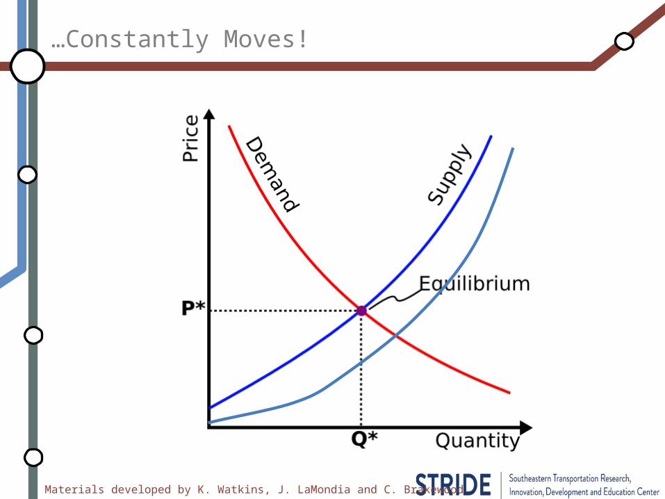
The Equilibrium Point…


…Constantly Moves!


Example 1

The travel time on a transit route from a major neighborhood to the downtown area has been observed to follow a supply trend of:

The demand trend for travel between the two areas is:

Determine the equilibrium travel time and passenger volume that will result on this route.

Assume time is in generalized minutes and volume is in passengers per hour.


Example 2

If the transit agency wants to add in a 5 minute layover at a stop & ride between the neighborhood and the city center, what impact will that have on ridership?


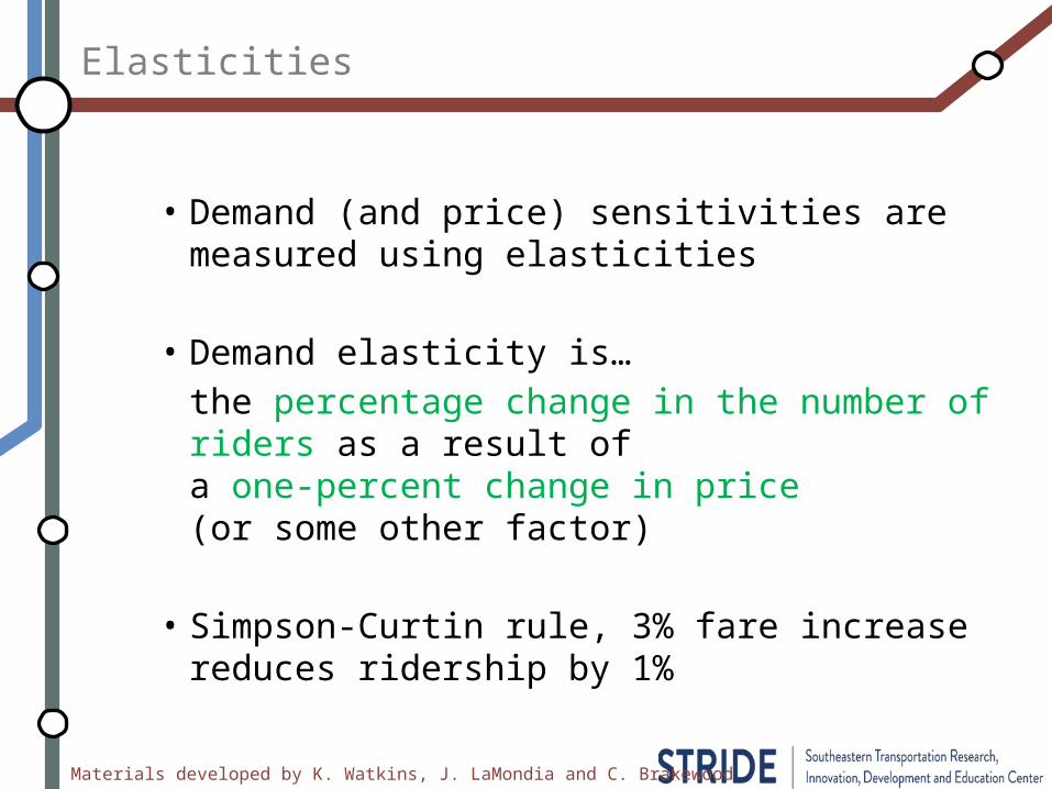
Elasticities

• Demand (and price) sensitivities are measured using elasticities

• Demand elasticity is…the percentage change in the number of riders as a result of a one-percent change in price (or some other factor)

• Simpson-Curtin rule, 3% fare increase reduces ridership by 1%


Elasticity Equation


Elastic/ Inelastic Threshold

• Range from -∞ to +∞+ indicates an increase in ridership due to the 1%

factor change- indicates a reduction in ridership due to the 1%

factor change

<|1| indicates inelasticity, with little impact>|1| indicates elasticity, with high impact


Cross-Elasticities


Example 1

Estimate the ridership elasticity for a park-ride shuttle service based on results from a cost-change experiment. Is it elastic?

The shuttle currently operates with 15 minute trips and serves 45 people during the peak hour. When these people were asked if they would continue using the service if trips were made every 20 minutes, 36 said they would.


Example 2

Estimate the ridership cross-elasticity for a park-ride shuttle service based on results from a cost-change experiment. Is it elastic?

When the same people were asked if they would continue using the service if the time it took to drive directly to the terminal was reduced from the current 30 minutes to 20 minutes, 25 agreed to stay with the park-ride shuttle service.


Demand Forecasting: The 4-Step Method

Trip Generation

(Frequency)

Trip Distribution

(Destination)

Mode Split(Mode)

Traffic Assignment

(Route)


Collect Data Describing a Specific Area

Predict % of Transit Riders

Predict Total # Travelers

Determine the Total # of Transit Riders per Timeframe

Predict # Transit RidersPredict # Transit Riders

Methods for Forecasting Demand


Two Approaches

System Demand Approach• Individual/ Aggregate

• Large Spatial Scale– Typically a city or region

• Policy/ Choice Analysis– Mode choices– Influence on congestion

Route Level Demand Approach

• Aggregate

• Local Spatial Scale– Typically a route or stop

• Volume Analysis– Stop arrivals– Rail system studies– Ridership along route


Collect Current/ Past Behavior &

Characteristic Data

Collect/Project Future Characteristic Data

Predict Future Behavior

Apply Demand Model to Future Characteristic Data

Estimate Relationships Between Characteristics

& Behavior

(DEMAND MODEL)

General Demand Forecasting Process


Data Collection

System Demand Approach• O-D Survey

• Region level estimates and assumptions for the future growth

Route Level Demand Approach

• Route Opinion Survey

• Route only estimates and assumptions for future growth


Factors Affecting Demand

• Service related variables tend to overwhelm demographic and employment factors– Fare costs– Travel times– Wait times– Access/ egress distances


SDA: Predicting Total # of Travelers

• Use information about a region to predict the number of total travelers from that region– Considers all modes


Cross-Classification & ITE Trip Generation

• Identify land uses and predict trips generated from these land uses

• Three techniques:– Rate, Regression, Match


Example of ITE

• We have a beachside townhome resort for 800 people being developed. The community will be served by rail, ferry and bus service, and we expect all the residents to use these modes. Calculate the total number of travelers we can expect during the AM peak period.


Example of ITE


SDA: Predicting % of Transit Riders

• Use information about modes to predict the share of travelers that will take transit– Considers CHOICE among all modes


Discrete Choice Models

• Based on utility of each option:

• NOTE: Always uses a base case, with a relative utility of zero


Discrete Choice Models

• Predict share based on relative utility of each mode:


Example

• Calculate the shares of travelers that choose Rail, Bus, or Ferry.


SDA: Predicting # of Transit Riders

• Combine number of travelers and share using transit to generate total number of travelers on a route


Example

• Calculate the number of people that we can expect on each of the transit options from the beachside community.


RLDA: Predicting # of Transit Riders

• Use information about a region to predict the exact number of transit riders on a given route– Gets straight to the number we’re looking for– Requires detailed route estimation– Usually site specific


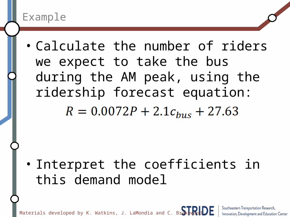
Example

• Calculate the number of riders we expect to take the bus during the AM peak, using the ridership forecast equation:

• Interpret the coefficients in this demand model


Which Method for Understanding Ridership is BEST?

• It all depends...– How much information do you have?– How accurate is your analysis?– What is the scale of your analysis?– How will it be used?


An EXAMPLE


Conclusion

• Incentives to ridership depend and the population, the geographic area, and the time of day.

• It is important to determine travel demand to plan for future service.

• The elasticity of demand is the marginal increase in ridership as a function of improved service or decreased price.


Reference

Materials in this lecture were taken from:• National Transit Database, U.S. Energy

Information Administration's Gas Pump Data History, and Bureau of Labor Statistics' Employment Data.

• Arrington, G. B., and Robert Cervero. "TCRP Report 128: Effects of TOD on Housing, Parking, and Travel." Transportation Research Board of the National Academies, Washington, DC 3 (2008).

• ITE, “Trip Generation Manual”

Materials developed by K. Watkins, J. LaMondia and C. Brakewood Understanding Changes in Ridership...

Documents

Transcript of Materials developed by K. Watkins, J. LaMondia and C. Brakewood Understanding Changes in Ridership...