Linearization in Electrical Impedance Tomography · Abstract This thesis considers a mathematical...

Linearization in

Electrical Impedance Tomography

Master’s Thesis

Author

Kristoffer Hoffmann

Supervisor

Kim Knudsen, DTU Mathematics© 17th June 2011 by Kristoffer Hoffmann

Technical University of Denmark

Linearization in


Kristoffer Hoffmann (s062116)

Abstract

This thesis considers a mathematical and numerical treatment of an inverse problemfrom electrical impedance tomography, which provides a framework for reconstructing aconductivity perturbation using electrical boundary measurements. Through linearizationof the classical conductivity equation, Calderon’s method is used to prove uniquenessof the linearized Neumann-to-Dirichlet (NtD) map in Rn, n ≥ 2 when the backgroundconductivity is homogeneous. Using complex geometrical optics solutions and a corres-ponding Schrodinger equation, a uniqueness result is also proved for the original non-linearNtD map in Rn, n ≥ 3. A similar uniqueness result, based on the Schrodinger equation in ahomogeneous background conductivity, is stated for the linearized NtD map in Rn, n ≥ 2.The linearised formulations are evaluated by a numerical implementation, which providesa method to reconstruct the conductivity perturbation in simple geometries. It is demons-trated that the numerical implementation is capable of reconstructing perturbation withan acceptable accuracy in both position and value, even if the boundary measurementsare affected by noise. If the exact shape and the approximate value of the perturba-tion is known, it is shown to be advantageous to linearize around a non-homogeneousbackground conductivity. If the exact shape of the perturbation is not known, the bestresults are found using a homogeneous background conductivity. The thesis ends with adiscussion of the implementation and suggestions for further development.

i

Preface

This report is the result of a master’s thesis project carried out at the Technical Uni-versity of Denmark (DTU) and it is the last part of the Master of Science programmein Mathematical Modelling and Computation. It is the result of around four and a halfmonths of work and is credited with 30 ECTS points. The work presented in this thesishas been done at DTU Mathematics during the period 1st February - 17th June 2011under the supervision of Kim Knudsen.

During the writing of this thesis, I have benefited from discussions and remarks fromvarious individuals. I would specially like to thank my supervisor Kim Knudsen for ourweekly meetings, interesting discussions and valuable feed-back. I also wish to thankthose of my fellow students who have contributed with important questions, commentsor remarks. Finally, I would like to thank my family and friends for their support andinterest.

I hope you will enjoy my thesis.

Kristoffer HoffmannKgs. Lyngby

June 2011

iii

Contents

Abstract i

Preface iii

Introduction ix

Reading Guide . . . . . . . . . . . . . . . . . . . . . . . . . . . . . . . . . . . . ix

1 Electrical Impedance Tomography 1

1.1 What is Electrical Impedance Tomography? . . . . . . . . . . . . . . . . . 1

1.1.1 Development History . . . . . . . . . . . . . . . . . . . . . . . . . . 1

1.1.2 Perspective and Current use of EIT . . . . . . . . . . . . . . . . . 2

1.1.3 Current Development . . . . . . . . . . . . . . . . . . . . . . . . . 2

1.2 The Mathematical Model . . . . . . . . . . . . . . . . . . . . . . . . . . . 3

2 The Forward Problem 7

2.1 Weak Derivatives and Sobolev Spaces . . . . . . . . . . . . . . . . . . . . 8

2.1.1 Weak Derivatives . . . . . . . . . . . . . . . . . . . . . . . . . . . . 8

2.1.2 Sobolev Spaces . . . . . . . . . . . . . . . . . . . . . . . . . . . . . 9

2.2 Weak Formulation . . . . . . . . . . . . . . . . . . . . . . . . . . . . . . . 10

2.3 Definition of Solution Space . . . . . . . . . . . . . . . . . . . . . . . . . . 11

2.4 Existence and Uniqueness . . . . . . . . . . . . . . . . . . . . . . . . . . . 12

3 The Classical Linearization Method 15

3.1 Perturbation Analysis . . . . . . . . . . . . . . . . . . . . . . . . . . . . . 17

3.2 Linearization - The Frechet Derivative . . . . . . . . . . . . . . . . . . . . 19

v

Preface

3.3 Uniqueness of the Linearized Inverse Problem . . . . . . . . . . . . . . . . 22

3.4 Reconstruction Using the Fourier Transform . . . . . . . . . . . . . . . . . 24

4 Complex Geometrical Optics Theory 27

4.1 The Schrodinger Equation . . . . . . . . . . . . . . . . . . . . . . . . . . . 27

4.2 CGO Solutions . . . . . . . . . . . . . . . . . . . . . . . . . . . . . . . . . 28

4.2.1 Existence and Uniqueness . . . . . . . . . . . . . . . . . . . . . . . 28

4.2.2 Exponential Solutions . . . . . . . . . . . . . . . . . . . . . . . . . 30

4.2.3 Zero Potential Solutions . . . . . . . . . . . . . . . . . . . . . . . . 31

4.2.4 Non-zero Potential Solutions . . . . . . . . . . . . . . . . . . . . . 32

4.2.5 Construction of CGO Solutions . . . . . . . . . . . . . . . . . . . . 33

4.3 Uniqueness of the Inverse Conductivity Problem . . . . . . . . . . . . . . 34

5 Linearization Using the Schrodinger Equation 39

5.1 Perturbation Analysis . . . . . . . . . . . . . . . . . . . . . . . . . . . . . 39

5.2 Linearization - The Frechet Derivative . . . . . . . . . . . . . . . . . . . . 41

5.3 Uniqueness of the Linearized Inverse Problem . . . . . . . . . . . . . . . . 44

5.4 Reconstruction Using the Fourier Transform . . . . . . . . . . . . . . . . . 45

6 Reconstruction of the Perturbation 47

6.1 Implementing the Forward Problem . . . . . . . . . . . . . . . . . . . . . 48

6.2 Discretization of the Classical Linearization . . . . . . . . . . . . . . . . . 48

6.2.1 Discretization of the Interior . . . . . . . . . . . . . . . . . . . . . 49

6.2.2 Discretization of the Boundary . . . . . . . . . . . . . . . . . . . . 51

6.2.3 The Linear System . . . . . . . . . . . . . . . . . . . . . . . . . . . 51

6.3 Solving the Linear System . . . . . . . . . . . . . . . . . . . . . . . . . . . 52

6.4 Discretization of the Schrodinger Linearization . . . . . . . . . . . . . . . 53

6.5 Summary - A Recipe for Reconstruction . . . . . . . . . . . . . . . . . . . 54

7 Results 55

7.1 The Procedure . . . . . . . . . . . . . . . . . . . . . . . . . . . . . . . . . 55

7.2 A Simple Problem . . . . . . . . . . . . . . . . . . . . . . . . . . . . . . . 56

vi

Preface

7.3 Position of the Perturbation . . . . . . . . . . . . . . . . . . . . . . . . . . 57

7.4 Effect of Noise . . . . . . . . . . . . . . . . . . . . . . . . . . . . . . . . . 58

7.5 Reconstruction Using the Schrodinger Linearization . . . . . . . . . . . . 61

7.6 Multiple Perturbations . . . . . . . . . . . . . . . . . . . . . . . . . . . . . 62

7.7 Non-homogeneous Background Conductivity . . . . . . . . . . . . . . . . . 63

7.7.1 A Single Perturbation . . . . . . . . . . . . . . . . . . . . . . . . . 64

7.7.2 Multiple Perturbations . . . . . . . . . . . . . . . . . . . . . . . . . 64

7.8 Non-homogeneous Background Conductivity with Wrong Shape . . . . . . 66

7.8.1 A Single Perturbation . . . . . . . . . . . . . . . . . . . . . . . . . 67

7.8.2 Multiple Perturbations . . . . . . . . . . . . . . . . . . . . . . . . . 68

Discussion and Perspectives 71

Conclusion 73

Appendices 75

Appendix A . . . . . . . . . . . . . . . . . . . . . . . . . . . . . . . . . . . . . . 75

A.1 Proof of Theorem 4.1 . . . . . . . . . . . . . . . . . . . . . . . . . 75



Appendix B . . . . . . . . . . . . . . . . . . . . . . . . . . . . . . . . . . . . . . 81

B.1 The NtD Map from a 2D Problem in a Homogeneous Medium . . 81

B.2 The NtD Map from a 2D Problem in an Inhomogeneous Medium 82

Appendix C . . . . . . . . . . . . . . . . . . . . . . . . . . . . . . . . . . . . . . 86

C.1 The Code for Building the Linear System . . . . . . . . . . . . . . 86

C.2 The Code for Solving the Linear System . . . . . . . . . . . . . . . 90

List of Symbols 91

Bibliography 93

vii

Introduction

This master’s thesis is carried out as a project related to the mathematical formulation ofelectrical impedance tomography (EIT), which is an imaging technique that exploits thedifference in electrical properties to reveal details about the inner structure of a medium.It explains in detail a mathematical and numerical treatment of EIT and is targeted atanyone who has interest in EIT or similar types of inverse problems.

The ambition of this thesis is to formulate the mathematical description of EIT, with focuson the inverse problem of finding the inner conductivity distribution using knowledge ofmeasurable electrical quantities on the boundary of some body. The objective is to derivesome of the most important theoretical results within the area. As this thesis will considerthe situation where a known current is applied on the boundary, the theory has to beformulated in relation to the so-called Neumann-to-Dirichlet map.

Besides treating the classical linearization of the inverse problem, a corresponding Schrodin-ger equation will be derived. The so-called complex geometrical optics theory will alsobe considered, since another objective is to state uniqueness for the inverse problem inthe original non-linear formulation. Furthermore, uniqueness of the linearized Schrodin-ger formulation will be stated. This linearization is particularly interesting since, to myknowledge, results using the linearization based on the Schrodinger formulation has notbeen published yet.

Since both linearizations offer the advantage of a simple numerical implementation of theinverse problem, it could be interesting to test the methods on a variety of problems toverify its accuracy and stability. A numerical implementation would also make it possibleto investigate how well EIT works as a method to reconstruct the internal conductivity. Anobjective is therefore also to produce a numerical implementation which can reconstructthe perturbation from various simple problems. As the inverse problem is severely ill-posed, it would be satisfactory if the reconstruction captures the approximate size, shapeand location of the perturbation.

Reading Guide

The thesis consists of seven chapters. The first five chapters consider the theoreticalresults, while Chapter 6 and 7 consider the numerical implementation of the inverseproblem. Some of the chapters can be read independently, but it is recommended to readthem in sequential order, as some of the chapters may use theory and notation defined inthe previous chapters.

ix

Introduction� Chapter 1: Makes the reader familiar with EIT and gives a brief explanation of thetechnique, the history and the areas of current research.� Chapter 2: Much of the physical and mathematical framework is established anduniqueness and existence for the forward problem is proved.� Chapter 3: Is related to the classical work in EIT due to Calderon’s famous paper [1].In this chapter the classical linearization method will be presented along with someimportant proofs. The most important proof states uniqueness of the NtD operatorin the linearized framework.� Chapter 4: The more advanced CGO theory is introduced. This makes it possibleto proof that the original non-linear NtD map uniquely determines the conductivityin three dimensions or higher.� Chapter 5: A linearization using the Schrodinger framework is presented. The chap-ter ends with a proof stating that also the Schrodinger linearization uniquely deter-mines the conductivity in at least two dimensions.� Chapter 6: Describes the construction of a numerical implementation of two recons-truction algorithms each based on the results from Chapter 3 and Chapter 5. It alsoincludes a thorough explanation of the mathematical and numerical methods usedin the implementation.� Chapter 7: The results from a reconstruction algorithm is presented. The methodis tested on a wide range of simple problems and the results from both algorithmsare presented.

A discussion of both the theoretical and the numerical results follows Chapter 7, alongwith suggestions on how to improve the numerical implementation. Also this section willgive some personal thoughts about the perspective and areas for further development inEIT. Finally, there is a conclusion, giving a summary of the theoretical and numericalresults and stating some final thoughts based on the work presented in the thesis.

In addition some supplementary material is placed as appendices. These contains proofsthat are too long to include in the text, an example of analytic NtD maps, and the sourcecode of the reconstruction algorithm. Furthermore, a list of the most used symbols isavailable on page 91.

x

Chapter 1


The following sections will introduce the reader to electrical impedance tomography(EIT). A description of the important events during the development of the methodsince the late 70’s, will follow a brief introduction to how the method works. Also someexamples of applications will be presented. The problem will at first be considered from aphysical perspective which will explain some of the physical mechanisms behind the tech-nology. In the end of the chapter, a mathematical model describing the relevant physicalquantities will be derived from Maxwell’s equations.

1.1 What is Electrical Impedance Tomography?

b

bb

b

bb

b

bb

bb b b

VI

Figure 1.1: An example on an ob-ject having an inclusion with dif-ferent conductivity. In EIT one mea-sures the current and electric poten-tial using electrodes placed on the boun-dary. These measurements are done oneach electrode and are used to recons-truct the internal conductivity distribu-tion.

Electrical impedance tomography is a non-invasiveimaging method giving information about the in-ternal conductivity distribution of an object. In anexperimental setup, conducting electrodes are pla-ced on the surface of the object and an electricalcurrent is applied and the resulting electric poten-tial is measured or vice versa, see Figure 1.1. Thesemeasurements are often repeated using different ap-plied currents or potentials and different electrodepositioning. The challenge in then to reconstructthe internal conductivity only using the measuredsets of current and potential data.

1.1.1 Development History

The first description of an imaging method basedon the principles of EIT is often attributed to RossP. Henderson and John G. Webster. In their paperfrom 1978 [2], they use the combination of voltageand current measurements to investigate the inter-nal thoracic region. Their paper mainly discussed

1

Chapter 1 Electrical Impedance Tomography

the instrument specifications and application procedures without giving much mathema-tical insight. In 1980 Alberto Pedro Calderon wrote a pioneer contribution to the Seminaron Numerical Analysis and its Applications to Continuum Physics in Rio de Janeiro [1].Calderon’s motivation was oil prospecting, as he worked in the state oil company of Ar-gentina in the 40’s [3]. This paper described a mathematical problem corresponding toan EIT measurement, that is if the conductivity inside an object can be determined byboundary measurements alone. Calderon did not fully answer this question in the paper,but under certain assumptions and simplifications he proved that when using a first orderlinearization, the relationship between the Dirichlet and Neumann boundary data coulduniquely determine the internal conductivity. In this scenario, he also proposed a solutionmethod to the inverse problem based on the Fourier transformation. After Calderon’spaper, the early development of the mathematical treatment of EIT slowly began. Someof the first important articles were published by Cheney, Kohn, Somersalo, Vogelius andD. and E. Isaacson in the late 80’s and 90’s. Also many important mathematical resultshas been made by Uhlmann and Sylvester, especially on uniqueness of the inverse pro-blem. As Calderon’s paper has been the underlying basis for the mathematical treatmentof EIT, many of the following chapters will be based of the thoughts and methods firstpresented by Calderon.

1.1.2 Perspective and Current use of EIT

The method has increasingly gained interest among scientist, engineers and in the me-dical industry in recent years. In the field of non-invasive imaging methods, it looks asa promising new technique usable in many different applications. Even though the usesprimarily are focused on the medical aspect, i.e. revealing, diagnosing, examining or stu-dying diseases, the procedure is not limited to medical applications and has potential ina broad range of disciplines. Sensoring, monitoring and control is often relying on bulky,inflexible and expensive apparatus like CT- or MR-scanners. Compared to the these tech-nologies, EIT is much more versatile and less expensive. As an example companies doingprospecting of oil or minerals could also benefit from such technological developments.They are dependent on flexible and large scale imaging techniques and from a techno-logical perspective, there is nothing preventing EIT from being used in such large-scalesetups. Many other industries can also benefit from this technology, as it can be used toexamine materials for internal contamination, cracks or similar defects. It can also workas an non-invasive way to inspect an intentionally made internal design, which in othercases is non-visible. Similar methods are also being developed for the use in geophysics forprospecting and in archaeology. In these fields the method is often known under namesas Electrical Resistivity Tomography, Electrical Resistance Tomography and ElectricalCapacitance Tomography [4].

1.1.3 Current Development

The process of reconstructing the internal conductivity is not very simple. Even though,it is clear from Ohm’s law that the relationship between the current and the potentialis in some way dependent on the internal conductivity, it is unclear if this relationshipuniquely defines the conductivity and if this is not the case, is it still possible to draw anyconclusion from the reconstruction? In some simple geometries and using approximation,

2

The Mathematical Model Section 1.2some results of uniqueness and existence have been made [4]. For instance, Kohn andVogelius proved that the conductivity distribution in dimensions n ≥ 2, can be uniquelydetermined from complete boundary measurements in situations where the boundary issmooth and the conductivity distribution is piecewise analytic [5]. One can also showunique determination of an isotropic conductivity (in C2) in dimensions n ≥ 3 [6]. Wewill treat this proof in Chapter 4 when we consider the so-called CGO solutions.

In this century much interest has been on problems where only data from a proper subsetof the boundary is available, cf. [7–9]. This so-called partial data problem is a veryimportant area in the current development as in many practical applications only partialdata is available. Also recently a family of direct non-linear solution techniques has beendeveloped for 2D models [10]. These so-called ∂-methods or scattering transform methodsare based on a uniqueness result stated by Nachmann in 1996 [11]. The hope is that thesemethods can be extended to three dimensional algorithms, making it possible to make afast 3D non-linear reconstruction on modest computers [4].

Many fields of EIT are yet to the investigated. Since Calderon’s fundamental paper startedthe mathematical analysis, these problems originating from EIT has been investigated bymathematicians, both theoretically and numerically, and still today the many questionshas not been answered due to the complexity of the severely ill-posed inverse problem.

1.2 The Mathematical Model

When dealing with a real physical problem, like EIT, the mathematical description isestablished using certain physical considerations and approximations. The mathematicalinsight often benefits from getting an understanding of the physical aspects which are of-ten hidden in the purely mathematical representation. Therefore this section starts witha brief explanation of the physical mechanisms underlying the later introduced mathema-tical theory. We first need to identify which measurable physical quantities are relevant.Then we need to state the behaviour of each physical quantity using some known mathe-matical description. By combining this information and taking into account the a prioriinformation available of the system, a mathematical model of the electrical potential insidea conducting medium having an applied current on the boundary is developed.

From a physical perspective the important quantities are the current and potential on theboundary, along with the electric potential, as the conductivity relates the current densityand the electric potential inside the medium. On the boundary the electrodes applies acurrent flux inside the medium and this flux excites the medium and giving rise to anelectric field. Dependent on the material, the size and direction of this field can be verydifferent. This field is related to the electric potential throughout the medium, and it isthis potential that is measured on the boundary.

Using mathematical modelling it is possible to describe the relationship between thesequantities and fields. In the following a mathematical model of EIT is derived takinginto account the physical considerations presented previously. Looking at the problemfrom a physical setting all fields are a consequence of the applied boundary current onthe boundary, and it will therefore be reasonable to consider this phenomenon first inthe modelling process. However, we start in kind of the opposite direction by deriving anequation for the electrical potential. This is due to the fact the Maxwell’s equations are so

3


fundamental in the field of electrodynamics and electrostatics that it would be a naturalplace to start. Afterwards we consider the applied current as it will work as a boundarycondition and as usual it will follow after the definition of the differential equation.

Consider a conducting body U , an open bounded subset of Rn, n ≥ 2 with a smoothboundary ∂U . In real-life applications one would consider R2 or R3. For a physical modelincluding potentials, currents or similar electrical quantities, the mathematical descriptionis very often based on Maxwell’s equations. According to Ampere’s circuital law themagnetic field intensity H and the electric field E are related as

∇×H = J + ε∂E

∂t,

where ε is permittivity of the medium and J the total current density. For the sake ofsimplicity the dependence of the spatial variable x is not and will in the following notalways be written explicitly. For the same reason, units of physical quantities are omitted.

Usually when modelling EIT is sufficient to consider the electrostatic problem. This comesfrom the fact that EIT operates at low frequencies in regimes of relatively low admittivityand short lenght scales [12–14]. In return the electric field becomes static and the equationsimplifies to

∇×H = J .

By definition the divergence of the curl of any vector field is equal to zero. This also holdsfor Ampere’s circuital law under for the assumption of no sources or sinks of current inU . This is in agreement with the application of EIT as the electrical excitation of themedium is only due to applied currents at the boundary. It follows that

∇ · (∇×H) = 0 ⇐⇒∇ · J = 0. (1.1)

A common approximation is that the electric field is proportional to the current density

J = γE,

where γ is the admittivity of the medium [13]. This makes it possible to express (1.1) as

∇ · γE = 0. (1.2)

The properties of the examined conducting materials are described by the admittivity.Physically this is the reciprocal of the electric impedance, hence the name electrical impe-dance tomography. In this thesis the case of isotropic admittivity is considered, meaningγ is not directional dependent and the admittisvity is also considered to be frequencyindependent. An isotropic conductivity makes the admittivity equal the electrical conduc-tivity. In many real-life situations the conductivity is in fact anisotropic. An example ofa medium with an anisotropic conductivity could be a layered medium originating froma crystalline structure or a deformation of an isotropic material [4]. Besides the morecomplex mathematical formulation, a reason for working in the isotropic formulation, isthat an anisotropic conductivity cannot be determined uniquely using the boundary mea-surements [4, 15]. For a treatment of the complex case having anisotropic and frequencydependent admittivity, see [13].

4

The Mathematical Model Section 1.2The model is also limited to strictly positive and bounded conductivities. A physicalmodel dealing with negative conductivity or describing the use of EIT on an infinitelygood conductor (a superconductor) is nowhere near the scope of this thesis. To keep thenotation simple we introduce the space L∞

+ (U) consisting of the strictly positive functionsin L∞(U) having the norm of the usual L∞-space. As γ is strictly positive and boundedwe can write γ ∈ L∞

+ (U) .

At this point we have no information about how the electric fieldE is related to the electricpotential. Going back to Maxwell’s equations, the Maxwell-Faraday equation (also knownas Faraday’s law of induction) states that

∇×E = −µ∂H

∂t,

where µ is the permeability of the medium. Again, because EIT operates at low frequenciesin regimes of relatively low admittivity and short lenght scales, the right-hand term canbe neglected. Thus,

∇×E = 0,

meaning that the electric field is conservative. As a result the scalar electrical potentialu is defined as the negative gradient of the electrical field and (1.2) simplifies to

∇ · γ∇u = 0, in U. (1.3)

This equation describes the electric potential inside the examined medium. We now needto describe the electrical excitation of the medium due to the applied current flux nor-mal to the boundary electrodes. The combination of these electrodes produces a currentdensity on the surface, where the outward pointed normal component g can be describedusing a unit outer normal vector ν at the boundary as

γ∂u

∂ν= g, on ∂U. (1.4)

In practice, this current density is what is being applied and in mathematical terms, fora known function g, this would be equivalent to having a Neumann boundary condition.Using Kirchhoff’s current law there should be conservation of charge on the boundary, thusthe mathematical description only makes sense for functions g satisfying

∫

δUg dS = 0 [16],

where dS is the usual surface measure on ∂U . Furthermore, one would have to choose areference potential. Mathematically this is clear from the formulation as u only appearin some derivative form in the PDE (1.3) and the boundary condition (1.4). Hence, anysolution u is only defined up to an additive constant. To circumvent this, usually u ischosen such that

∫

δUu dS = 0. This would be the same as defining the boundary as

”ground” [13].

To sum up, the problem in question can mathematically be formulated as

∇ · γ∇u = 0, in U,

γ∂u

∂ν= g, on ∂U,

(1.5)

where γ ∈ L∞+ (U),

∫

δU u dS =∫

δU g dS = 0 and U is an open bounded subset of Rn, n ≥ 2with smooth boundary ∂U having outer normal unit vector ν. This model is often called

5


the continuum model [13], and this model is clearly a simplification of real life. As anexample it leaves out the effect of the electrodes positioned on the boundary as themodel assumes the the current is known in all points of the boundary. Other models havebeen proposed like the gap model which approximates the current density as constant oneach electrode and zero in the gaps between the electrodes. This model was shown tobe inaccurate by Isaacson and Cheney in [17]. Another model of the boundary current,the complete electrode model [18], uses a much more advanced way of modelling theeffect of the electrodes. It has been shown that this model is capable of predicting theexperimentally measured voltages with an error as little as 0.1 % [19]. This model isnot used in the following, since the mathematical description is very complex, but boththeoretical and numerical results exist [20, 21].

6

Chapter 2

The Forward Problem

Having a physical setting, the problem is very often to investigate the effect of some knowncause. An example could be to derive an expression for the electric field around someelectrically charged particles. It is usually based on some known model parameters (thecause) resulting in some analytical expression or numerical data (the effect) which thenwould be verified by experiments. Also for historical reasons this type of problem is usuallyconsidered to be fundamental and has therefore been investigated more exhaustively. Sucha problem, of finding the effect of a known cause, is often called a direct problem or aforward problem. Correspondingly, the opposite problem, seeking the cause of some effect,is in a physical setting often called an inverse problem. An example of this could be theproblem of determining the position of some electrically charged particles giving rise toa known electric field. This type of problem is usually much more difficult to solve andmany possible solutions exist. There exists no precise definition of when a problem is aninverse problem, but often one defines two problems to be inverses of one another if theformulation of each involves all or part of the solution of the other. Also if one of the twoproblems has been studied extensively for some time, it is commonly called the forwardproblem [22].

The classical PDE analysis has repeatedly been motivated by the question of finding so-lutions to problems similar to the one presented in the previous chapter. Usually this isdone under the assumption of full knowledge of γ and g. Indeed, this is often the cor-rect mathematical interpretation of the real-life problem at hand. In many cases one isinterested in determining some physical field or quantity based on some known physicalparameters and a known geometry. Using the definition by Keller [22], this is then theforward problem. However, in the case of EIT, one wants to reconstruct the conducti-vity γ from knowledge of boundary measurements alone. Therefore the reconstruction ofthe conductivity used in the mathematical formulation of EIT is considered an inverseproblem.

Even though this thesis will mainly focus on the inverse problem, the two types of problemsare closely related. The forward problem will be treated in the following sections andthis will work as an introduction to the physical problem in question. It will also state,clarify and describe some important topics which are necessary in order to understand theinverse problem. Using the definition and concepts that are introduced in the following,the objective of this chapter is to show existence and uniqueness of solutions to the forward

7

Chapter 2 The Forward Problem

problem in the so-called weak formulation.

2.1 Weak Derivatives and Sobolev Spaces

Having defined the mathematical problem, the treatment will now focus on solution me-thods. In this work, the concept of weak formulations will be considered. This method isvery common in the field of PDEs and it is also the main mathematical technique behindthe popular finite element method used in many mathematical software packages.

The problem (1.5) with γ being strictly positive, is an elliptic boundary value pro-blem [23]. The smoothness requirements indirectly introduced by the partial differen-tiations defining the boundary value problem often limits any possible solution to a set ofcontinuously differentiable functions of some order. The difficulty is that a classical boun-dary value problem, even if the formulation only includes smooth coefficients, may notadmit solutions of this type [24]. In the class of elliptic problems, this difficulty is oftenthe motivation behind weakening the smoothness requirements by rewriting the boundaryvalue problem at hand in some ”weaker” form. This will admit new types of solutions,which for instance are not differentiable in the classical sense. Leaving the classical PDEanalysis, gives access to the abstract tools of functional analysis which are found to bevery useful especially when dealing with elliptic boundary value problems. Before conti-nuing the treatment of (1.5), the important concepts of weak derivatives and the Sobolevspace H1(U) are defined.

2.1.1 Weak Derivatives

Weak derivatives are crucial in the understanding of the weak formulation. It is an exten-sion of the classical derivative to functions not being differentiable in the classical sense.To define the weak derivatives, the set L1

loc(U) must be considered. This set consists ofall functions in U which are integrable on any compact subset of U . Furthermore, we usethe usual notation to define C∞

c (U) as the set of smooth functions with compact supportin U . The following definition can then be stated.

Definition 2.1 (Weak Derivative)Suppose that U is an open bounded subset of Rn. Let u : U → C ∈ L1

loc(U)and ∇u : U → Cn ∈ L1

loc(U). Let ∂k denote the partial derivative in thek’th coordinate. The gradient operator is redefined such that ∇u is called theweak derivative of u, written

∇u = (∂1u, ∂2u, . . . , ∂nu)

provided∫

U

∂kuφdx = −∫

U

u∂kφdx

for all functions φ ∈ C∞c (U) and for all k = 1, 2, . . . , n.

8

Weak Derivatives and Sobolev Spaces Section 2.1� Remark It is clear from the definition that if u is differentiable then ∇uis a weak derivative. Also notice that the integrals involved are well-definedas φ and ∂kφ have compact support and thus only non-zero in a subset ofU , and since u and ∂ku are locally integrable it follows that the integrals areL1-integrable on such a subset. From the definition it also follows that allweak derivatives are equal almost everywhere, as any two weak derivatives∇1u and ∇2u would require

∫

U(∇1u−∇2u)φdx = 0 for all φ ∈ C∞

c (U).

2.1.2 Sobolev Spaces

When dealing with elliptic problems it is often advantageous to work with functions inthe so-called Sobolev spaces. A Sobolev space is a vector space of functions equipped witha norm consisting of the usual Lp-norm of the function itself along with weak derivativesof various orders. Depending on the problem at hand different Sobolev spaces shouldbe considered. In our case, the main focus will be the Sobolev space H1(U) as it is theappropriate choice for our type of problem.

Definition 2.2 (The Sobolev space H1(U))The Sobolev space H1(U) consists of all locally integrable functions u: U → C

such that ∇u exists (according to Definition 2.1) and u and ∇u belongs toL2(U).

If u ∈ H1(U) we define its norm by

‖u‖H1(U) :=

(∫

U

|u|2 + |∇u|2 dx

)12

.

With respect to the inner product

(u, v)H1(U) =

∫

U

u v +∇u · ∇v dx,

H1(U) is a Hilbert space [23].� Remark So far, no investigation of the uniqueness of ∇u has beenmade. In fact, several weak derivatives may exist and one might be confu-sed about which one to use in the definitions above. However, as all weakderivatives are equal up to a Lebesgue measure zero, they would all resultin the same norm and inner product for each u ∈ H1(U) as required.

Note that the additional requirement of a function u being in H1(U) rather than L2(U)

is∫

U|∇u|2 dx < ∞. Going back to the physical setting, this corresponds to the ohmic

power dissipated in U being finite, given a bounded conductivity [4]. From a physicalpoint of view, this requirement seems logical for any reasonable solution.

In the following we will often need the restriction of a function to the boundary in termsof the function values (Dirichlet data) or the boundary derivatives (Neumann data).

9


Although u might not be continuous, it is still possible to give meaning to the restrictionu|∂U for any u ∈ H1(U) by use of the Sobolev trace operator, if u is a solution to (1.5). Asthis treatment is quite advanced, the definition is stated below, but the proof is omitted.A treatment of trace operators in Sobolev spaces is not the scope of this thesis and werefer to [23] or [25] for more information.

For a continuous function, v : U → C the trace of v is simply the function restricted tothe boundary. However, in our case the function may not be differentiable in the classicalsense or it is only defined almost everywhere in U . As the choice of restriction to theboundary has no effect on the integrals involved in the definition of the space H1(U), theexpression ”u restricted to ∂U” has no direct meaning [23]. The trace operator solves thisambiguity and defines the restriction to the boundary for functions in Sobolev spaces. Fora function u ∈ H1(U) the operator maps into an L2 function on the boundary. In thiscase the operator can be defined using the following [23].

Definition 2.3 (The Trace Operator)Assume U is bounded and ∂U is C1. Then there exists a bounded linearoperator

T : H1(U) → L2(∂U)

such that

Tu = u|∂U if u ∈ H1(U) ∩ C(U)

and

‖Tu‖L2(∂U) ≤ C ‖u‖H1(U)

for each u ∈ H1(U), with the constant C depending only on U .

The function Tu is called the trace of u on ∂U .

In the following all restrictions to the boundary should be understood as being in thetrace sense, even if it is not written explicitly. It follows that we can write u|∂U ∈ L2(∂U)if u ∈ H1(U).

The classical treatment of the PDE would limit the solutions to C2(U). As we will see, thechoice of the solution space H1(U) follows directly by rewriting the problem in its weakformulation. However, any weak solution must satisfy an additional requirement. At thismoment it might not be clear, but it follows from the treatment of the weak formulation.

2.2 Weak Formulation

Now the basic concepts of weak derivatives and the Sobolev space H1(U) have beendefined and (1.5) can be reformulated in a weak form.

The PDE is first multiplied by a so-called test function φ ∈ H1(U). Then the equation is

10

Definition of Solution Space Section 2.3integrated over U to obtain

∫

U

∇ · γ∇uφdx = 0.

Now, Green’s first identity yields

∫

U

∇ · γ∇uφdx = 0 ⇐⇒∫

U

γ∇u · ∇φdx −∫

∂U

γ∂u

∂νφdS = 0 ⇐⇒

∫

U

γ∇u · ∇φdx =

∫

∂U

g φdS. (2.1)

As u and φ both are elements of H1(U), their gradients are in L2(U). Using the Cauchy-Schwarz inequality we see that

∫

U

γ∇u · ∇φdx = ‖γ∇u · ∇φ‖L1(U)

≤ ‖γ‖L∞(U) ‖∇u‖L2(U) ‖∇φ‖L2(U)

≤ ‖γ‖L∞(U) ‖u‖H1(U) ‖φ‖H1(U) .

Thus, the integral to the left in (2.1) is well-defined. The integral to the right has thefollowing bound

∫

∂U

g φdS = ‖g φ‖L1(∂U)

≤ ‖g‖L2(∂U) ‖φ‖L2(∂U) .

These are boundary integrals and φ should be considered as being the trace of φ. From thedefinition of the trace operator it follows that the trace of φ is an element in L2(∂U). Tomake sure ‖g‖L2(∂U) is bounded, we just choose our applied current density such that g

is an L2(∂U) function. As noted in Section 1.2, the mathematical description only makessense for functions g satisfying

∫

δUg dS = 0. The space of functions in L2(∂U) integrating

to zero is denoted by L2�(∂U). It is therefore a requirement that g ∈ L2

�(∂U). For anysolution to the original problem, (2.1) must be true for all φ ∈ H1(U). Any solution uthat satisfies the integral equation above for all φ ∈ H1(U) is denoted a weak solution to(1.5), as this type of solution might not be a solution in the classical sense.

Having the original problem written in its weak form, an appropriate solution space willnow be defined.

2.3 Definition of Solution Space

To make the solution match the requirements given by the boundary conditions, an ad-ditional restriction to the solution space is made. We now want to focus our search ofsolutions from the space H1(U) to functions also having vanishing integral mean on theboundary. Remember that this is a result of the defined reference electrical potential. This

11


space is usually denoted H1� (U) and consists of functions having the properties

H1� (U) =

{

u ∈ H1(U) :

∫

∂U

u dS = 0

}

,

and having the same norm and inner product as H1(U). Mathematically,∫

∂U u dS = 0should be understood as the trace of u integrates to zero along the boundary. Previouslyit was stated that for any weak solution u to (2.1), u|∂U is an element of L2(∂U). Sinceit also integrates to zero, we can now write u|∂U ∈ L2

�(∂U).

As previously stated, H1(U) is a Hilbert space. We now want to show that H1� (U) is

also a Hilbert space. Consider the restriction of zero integral means in terms of the linearbounded mapping l : H1(U) → C defined as

l : u 7→ 〈Tu, 1〉 ,

where 〈·, ·〉 denotes the usual L2(∂U) inner product being antilinear in the second argu-ment. To show it is a Hilbert space, it is clearly enough to show that any Banach seriesof functions satisfying the restriction, converges to a function which also satisfies the res-triction. This is true, since for any converging Banach series, uj → u satisfying l(uj) = 0,the limit function would also satisfy l(u) = 0 as the mapping l is continuous. This meansthat H1

� (U) is complete with respect to the restriction, hence a Hilbert space itself.

2.4 Existence and Uniqueness

The term to the left in (2.1) can be expressed by Bγ(u, v) : H1� (U)×H1

� (U) → C, definedas

Bγ(u, v) =

∫

U

γ∇u · ∇v dx, (2.2)

where the second input has been conjugated. This form is a sesquilinear form as it islinear in the first argument and anti-linear in the second input.

Often the Lax-Milgram theorem is used to prove the important fundamental conceptsof existence and uniqueness for solutions to elliptic problems. The Lax-Milgram theo-rem is an extension of the classical Riesz’ representation theorem to non-symmetric bili-near forms [23]. However, in our case the sesquilinear form (2.2) is conjugate symmetric,Bγ(u, v) = Bγ(v, u), hence it is straightforward to show uniqueness and existence usingRiesz’ representation theorem. It is only necessary to show that Bγ(u, v) defines an in-ner product on H1

� (U). This is proved by showing that it satisfies the following threeproperties [26].� Conjugate symmetry

As stated above, Bγ is clearly conjugate symmetric.� Linearity in the first argumentWe can conclude that Bγ is linear in the first argument, as both gradient and integraloperators are known to be linear.� Positive definitenessWe need to show that Bγ(u, u) =

∫

Uγ |∇u|2 dx is non-negative and only zero if

12

Existence and Uniqueness Section 2.4‖u‖H1

�(U) = 0. As the conductivity γ is assumed to be strictly positive in all ofU , the only difficulties arise when ∇u = 0 almost everywhere in U , which implies‖∇u‖L2(U) = 0. But in this case u is equivalent to a constant k in H1

� as ‖u −k‖H1

�(U) = 0. The requirement of∫

∂Uu dS = 0 in a trace sense implies k = 0, and

thus u is equal to zero in H1� (U). This shows positive definiteness of Bγ .

The integral functional Φ(v) =∫

∂Ug v dS is an anti-linear functional on the Hilbert space

H1� (U). As stated previously, Cauchy–Schwarz’ inequality shows that this is bounded for

g, v|∂U ∈ L2�(∂U). As shown above Bγ(u, v) defines an inner product on H1

� (U) and itfollows from Riesz’ representation theorem that there exists a unique u ∈ H1

� (U) suchthat the functional has a representation in the form of an inner product, Φ(v) = (u, v)for all v ∈ H1

� (U) [26]. Thus, we can write

(u, v) = Φ(v) ⇐⇒

Bγ(u, v) =

∫

∂U

g v dS,

which we recognize as the weak formulation (2.1). From this analysis it follows thatthe problem (1.5) has a unique weak solution u. This important result is stated in thefollowing theorem.

Theorem 2.4Let U be an open bounded subset of Rn, n ≥ 2 with a smooth boundary∂U . If γ ∈ L∞

+ (U) and g ∈ L2�(∂U) then (1.5) has a unique weak solution

u ∈ H1� (U).� Remark It follows directly by the weak formulation, that any strong

solution, that is a solution in the classical sense, is also a weak solution. Thisimplies that any unique solution to the weak formulation is also a strongsolution, if a strong solution exists. Thus, the extension to the weak formu-lation only gives ”new” solutions in situations where the classical formulationdoes not admit solutions.

Having defined the necessary mathematical concepts and shown existence and uniquenessof solutions to the conductivity equation, we continue the mathematical treatment of EIT.In the following chapter, the treatment of the inverse problem begins by considering theclassical linearization method. This makes it possible to show that, in a linearized case,the measured boundary data uniquely determines the conductivity.

13

Chapter 3

The Classical Linearization Method

Now we will turn our attention to the classical linearization method in EIT, first propo-sed by Calderon in his fundamental paper [1]. From a mathematical point of view, theobjective is to find some formulation of the connection between the measured boundarydata and the conductivity distribution. In the original paper Calderon considered the si-tuation where a known voltage was applied on the boundary and investigated the changein current due to a perturbed conductivity distribution. However, in the chapter the op-posite situation will be considered, i.e fixing the current and investigating the changein voltage. The reason is that this gives some smoothing features which are well-suitedfor noisy measurements [13]. Nevertheless, the mathematical derivation is very similar inboth cases.

To have a mathematical formulation of the link between the measured boundary data, theso-called Neumann-to-Dirichlet (NtD) operator is introduced. This is an operator mappingcurrent to voltages on the boundary. Think of it as a mapping converting Neumannboundary conditions to Dirichlet boundary condition, without changing the solution. Theformulation and notation are stated in the following definition.

Definition 3.1 (The Neumann-to-Dirichlet Operator)Let g ∈ L2

�(∂U), γ ∈ L∞+ (U) and u ∈ H1

� (U) be a weak solution to

∇ · γ∇u = 0, in U,

γ∂u

∂ν= g, on ∂U.

The Neumann-to-Dirichlet operator R is then for each γ a mapping

Rγ : L2�(∂U) → L2

�(∂U)

defined by

Rγg 7→ f,

where f = u|∂u ∈ L2�(U).

In mathematical terms, solving the problem having a Neumann boundary condition des-cribed by a function g, would be equivalent to solving the problem having a Dirichlet

15

Chapter 3 The Classical Linearization Method

condition u|∂U = Rγg. Besides being dependent on the geometry of the domain, the map-ping is dependent on the internal conductivity distribution γ in a non-linear way. Thus,for obvious reasons it is unrealistic to aim for an explicit mathematical expression of thisoperator. Instead, we focus on investigating how the operator changes for small changesin the conductivity for a fixed geometry. This matches real-life applications where the me-thod is used on fixed objects having a somewhat homogeneous conductivity distribution.For such applications it is also often sufficient for the method to provide an approximatelocalization or give a contrast between regions having different conductivity. In turns outthat the NtD operator is crucial in the process of reconstructing the internal conductivitydistribution.

It should be noted that Definition 3.1 provides very little information available about theproperties of the NtD operator. However, in specific situations, the NtD operator can beexpressed analytically. Two examples are available in Appendix B.1 and Appendix B.2where the NtD operator is derived in a homogenous and a non-homogenous circularmedium. It is recommended to look at the derivations as they may help to get an betterunderstanding of the concept of NtD operators. If the Neumann boundary conditions arecomplex exponentials, the analytical expressions for the NtD operators also show thatthe influence is largest from the lower order modes. This discovery is in fact importantfor the numerical implementation, which is treated in Chapter 7.

D

U\D

Figure 3.1: An example of an in-clusion having different conducti-vity than the surrounding mate-rial. The total conductivity γ isdifferent in the two regions.

Before investigating the behaviour of the NtD operator,we will make a more specific formulation of the problemin question. Again consider a conducting body U , anopen bounded subset of Rn, n ≥ 2 with a smooth boun-dary ∂U . Let γ0 ∈ L∞

+ (U) be a homogeneous ”back-ground” conductivity and let δ ∈ L∞(U) be a smallperturbation of the conductivity, only being non-zero insome inclusion D of the domain, see Figure 3.1. Thetotal conductivity is then defined as

γ = γ0 + δ.

Both γ0 and δ should be defined in such way that thetotal conductivity is strictly positive, i.e. γ ∈ L∞

+ (U).The problem is then to reconstruct the perturbation δusing only boundary measurements. It is assumed that γ0 is known and that the inclusionis limited to the interior of U .

As noted in Section 1.2, the governing equation is

∇ · γ∇u = 0, x ∈ U, (3.1)

along with a Neumann boundary condition

γ∂u

∂ν= g, on ∂U, (3.2)

and conservation of current on the boundary

∫

∂U

g dS = 0. (3.3)

16

Perturbation Analysis Section 3.1Note that γ in (3.2) actually is equal γ0 as the perturbation is limited to the interior ofU .

Using this setup, it seems reasonable to make a linearization to describe the behaviour ofRγ for small changes in γ. This somewhat easy perturbation calculation may seem fairlysimple, as one could just write up the change for a small perturbation and then removeall terms being second-order or higher in this perturbation. However, it turns out that amore thorough perturbation analysis in needed to determine in which order some termsdepend on the perturbation.

3.1 Perturbation Analysis

To simplify the notation, this analysis begins with the definition of a linear second orderdifferential operator.

Definition 3.2 (The Differential Operator Lγ)The differential operator Lγ is for each γ ∈ L∞

+ (U), u ∈ H1� (U) defined by

Lγu = ∇ · γ∇u.

Now, denote by H−1(U) the dual space of H1� (U). For any u∗ ∈ H−1(U) the dual norm

is defined as

‖u∗‖H−1(U) = sup‖φ‖≤1

|〈u∗, φ〉| , φ ∈ H1� (U),

where 〈·, ·〉 denotes the usual L2(U) inner product.

Let X and Y be two normed vector spaces. We denote by ‖·‖L(X,Y ) the usual X → Y

operator norm and by ‖·‖L(X) the usual X → X operator norm for bounded linearoperators. The following theorem states some properties of Lγ .

Theorem 3.3For each γ ∈ L∞

+ (U), Lγ is a mapping

Lγ : H1� (U) → H−1(U).

Furthermore ‖Lγ‖L(H1�(U),H−1(U)) → 0 as ‖γ‖L∞(U) → 0.

ProofLet u, φ ∈ H1

� (U). Then Lγ is a mapping from H1� (U) into its dual space

17


H−1(U). This follows from the fact that Lγ clearly is linear and

‖Lγu‖H−1(U) = sup‖φ‖

H1�(U)

≤1

|〈Lγu, φ〉|

= sup‖φ‖

H1�(U)

≤1

∣

∣

∣

∣

∫

U

(∇ · γ∇u)φdx

∣

∣

∣

∣

= sup‖φ‖

H1�(U)

≤1

∣

∣

∣

∣

−∫

U

γ∇u · ∇φdx +

∫

∂U

γ∂u

∂νφdS

∣

∣

∣

∣

≤ sup‖φ‖

H1�(U)

≤1

(

‖γ‖L∞(U) ‖u‖H1�(U) ‖φ‖H1

�(U) + ‖γ‖L∞(U)

∥

∥

∥

∥

∂u

∂ν

∥

∥

∥

∥

L2(∂U)

‖φ‖L2(∂U)

)

The inequality from Definition 2.3 can be applied, since φ|∂U is the trace ofφ, and the bound becomes

‖Lγu‖H−1(U) ≤ ‖γ‖L∞(U)

(

‖u‖H1�(U) + C

∥

∥

∥

∥

∂u

∂ν

∥

∥

∥

∥

L2(∂U)

)

,

where C is a constant only dependent on U .

This constant is a result of φ|∂U being the trace of φ and the right-hand side isclearly bounded for the functions considered. It follows that Lγu ∈ H−1(U),implying Lγ : H

1� (U) → H−1(U). From the bound it is also obvious that

‖Lγ‖L(H1�(U),H−1(U)) → 0 as ‖γ‖L∞(U) → 0.

Now assume that u ∈ H1� (U) is a solution to (3.1) without perturbation, then Lγ0u = 0.

Similarly, denote by v ∈ H1� (U) a solution to the problem with perturbation, then Lγv =

0. The difference between the two solutions is denoted w = v − u ∈ H1� (U). It follows

from the definition of Lγ that

Lγv = 0 ⇐⇒Lγ0u+ Lγ0w + Lδu+ Lδw = 0 ⇐⇒

Lγ0w + Lδu+ Lδw = 0. (3.4)

At this point the inverse of Lγ0 could come in handy. Now, first consider a problem ofthe type

∇ · γ0∇w = h, in U,

γ0∂w

∂ν= 0, on ∂U,

(3.5)

where γ0 ∈ L∞+ (U), γ0

∂w∂ν ∈ L2

�(U) and w ∈ H1� (U). Using integration by parts we note

that this only makes sense if∫

U h dx = 0. For all h ∈ H−1(U), this type of problem hasa unique solution w ∈ H1

� (U) [27]. Additionally for each h ∈ H−1(U) we get a bound onw such that

‖w‖H1�(U) ≤ C‖h‖H−1(U),

where C is a positive real constant [27].

Thus, we can define the operator that maps h ∈ H−1(U) into v ∈ H1� (U) as the Neumann

operator.

18

Linearization - The Frechet Derivative Section 3.2Definition 3.4 (The Neumann Operator Nγ)Consider a problem of the type (3.5). The Neumann operator Nγ0 :H

−1(U) →H1

� (U) is defined by

w = Nγ0h.

The Neumann operator satisfies

‖Nγ0‖L(H−1(U),H1�(U)) ≤ C,

where C is a positive real constant.

Since γ dwdν = 0, the Neumann operator can now be applied to (3.4) which gives

Nγ0Lγ0w +Nγ0Lδu+Nγ0Lδw = 0 ⇐⇒(1 +Nγ0Lδ)w = −Nγ0Lδu.

The question is now if the operator (1+Nγ0Lδ) is invertible. Let us for a moment assumethat it is invertible, then w can be expressed as a geometric series

(1 +Nγ0Lδ)w = −Nγ0Lδu ⇐⇒w = −(1 +Nγ0Lδ)

−1Nγ0Lδu ⇐⇒

w =

( ∞∑

n=1

(−Nγ0Lδ)n

)

u.

This can be recognized as a Neumann series. Hence, if ‖Nγ0Lδ‖L(H1�(U)) < 1 the operator

is invertible by Neumann’s theorem and the operator series will converge [28]. As operatormultiplication of linear bounded operators is jointly continuous,

‖Nγ0Lδ‖L(H1�(U)) ≤ ‖Nγ0‖L(H−1(U),H1

�(U))‖Lδ‖L(H1�(U),H−1(U)).

Using the bounds from Theorem 3.3 and Definition 3.4 it follows that if we choose δsmall enough ‖Nγ0Lδ‖L(H−1(U),H1

�(U)) < 1 as required and the operator is invertible. Thechange in inner potential w caused by the change in conductivity δ, can then be expressedusing the series as

w = −Nγ0Lδu+ (Nγ0Lδ)2u+ . . .

Using the analysis above it follows that ‖w‖H1�(U) = O(‖δ‖L∞(U)) for small ‖δ‖L∞(U),.

Hence, the change in norm of the potential is of the same order as the norm of the smallperturbation. This results makes it possible to linearize the inverse problem.

3.2 Linearization - The Frechet Derivative

As Calderon noted [1], it is advantageous to work with the quadratic form associatedwith Rγ .

19


Definition 3.5 (The Quadratic Form Qγ)The mapping Qγ : L2

�(∂U) → R is defined by the quadratic form

Qγ(g) = 〈g,Rγg〉.

In the definition above 〈·, ·〉 denotes the usual L2(∂U)-inner product, defined to be anti-linear in the second argument. The quadratic form can be used to express the weakformulation of the conductivity equation presented in Section 2.2.

Theorem 3.6Let u ∈ H1

� (U) be a weak solution to (3.1) without perturbation and letg = γ ∂u

∂ν ∈ L2�(∂U). Then

Qγ(g) = 〈g,Rγg〉 =∫

U

γ |∇u|2 dx.

From the results of Section 2.4 it follows that Rγ is determined by the unique weaksolution u. It is clear that if Rγ is known, Qγ is easy to determine using Definition 3.5.If Qγ is known, Rγ can be determined by defining a sesquilinear form and applying thepolarization identity. In other words knowing Rγ orQγ for all g ∈ L2

�(∂U) is equivalent [3].

Physically Qγ(g) is a measure of the power necessary to maintain the current g on theboundary [1]. From an experimental perspective, this is a more simple quantity to measurethan having to find a convenient way to prescribe boundary current measurements [29].However, this will not be used in this thesis as only the mathematical treatment is consi-dered and in this case the boundary data is just as simple to work with.

The quadratic form, Qγ is for each conductivity distribution given by the forward map

Q : L∞+ (U) → L(L2

�(∂U),R),

Q : γ 7→ Qγ .

This map is clearly non-linear as a change in γ would produce a different solution u andchange the term

∫

U γ |∇u|2 dx in a non-linear way. The ultimate goal would be to invertthis map, giving an expression for the internal conductivity distribution once Qγ (or Rγ)is known. However, due to the non-linear nature of the map, there is no simple methodto do this. Instead the linearized map is considered in order to determine the change inboundary data when the conductivity distribution is changed by a small perturbation δ.

At first, consider the change in Q when the conductivity is perturbed by δ. This quantitycan be expressed as

Qγ0+δ(g)−Qγ0(g) =

〈g,Rγ0+δg〉 − 〈g,Rγ0g〉 =∫

U

(γ0 + δ) |∇(u+ w)|2 dx−∫

U

γ0 |∇u|2 dx =

∫

U

[

δ |∇u|2 + (γ0 + δ) |∇w|2 + 2(γ0 + δ)Re(∇u · ∇w)]

dx,

20

Linearization - The Frechet Derivative Section 3.2where u,w ∈ H1

� (U) are defined as in Section 3.1 and Re(∇u · ∇w) denotes the realpart of ∇u · ∇w. From the perturbation analysis done in Section 3.1 it follows that‖w‖H1

�(U) = O(

‖δ‖L∞(U)

)

. This means that the integration of |∇w|2 and any product of

δ and ∇w are O(

‖δ‖2L∞(U)

)

. Hence,


∫

U

δ |∇u|2 dx+

∫

U

2γ0Re(∇u · ∇w) dx +O(

‖δ‖2L∞(U)

)

.

Using Green’s second identity on the second integral gives

∫

U

γ0Re(∇u · ∇w) dx = Re

(∫

U

γ0∇u · ∇w dx

)

= Re

(

−∫

U

∇ · γ0∇uw dx+

∫

∂U

γ0∂u

∂νw dS

)

= Re

(∫

∂U

γ0∂u

∂νw dS

)

= Re (〈g,Rγ0+δg〉 − 〈g,Rγ0g〉)= Qγ0+δ(g)−Qγ0(g),

as Qγ0+δ(g) − Qγ0(g) clearly is a real-valued quantity and ∇ · γ0∇u = 0 in U by thedefinition of u. It follows that


∫

U

δ |∇u|2 dx+ 2(Qγ0+δ(g)− (Qγ0)(g)) +O(

‖δ‖2L∞(U)

)

⇐⇒

Qγ0+δ(g)−Qγ0(g) = −∫

U

δ |∇u|2 dx+O(

‖δ‖2L∞(U)

)

.

The so-called Frechet derivative of the mapQ : L∞(U) → L(L2�(∂U),R), at γ0 in direction

δ is denoted by dQγ0 [δ](g). Using the definition from [30] the Frechet derivative satisfiesthe equation

Qγ0+δ(g)−Qγ0(g) = dQγ0 [δ](g) +O(

‖δ‖2L∞(U)

)

.

Thus, the Frechet derivative is just the first order term of change in the quadratic form

dQγ0 [δ](g) = −∫

U

δ |∇u|2 dx.

Usually this result is rewritten using the sesquilinear form Bδ defined below.

Definition 3.7 (The sesquilinear form Bδ)Let g1, g2 ∈ L2

�(∂U). Then the sesquilinear form Bδ is defined by

Bδ(g1, g2) =

∫

∂U

(Rγ0+δ −Rγ0)g1g2 dS.

As Bδ(g, g) = dQγ0 [δ](g)+O(

‖δ‖2L∞(U)

)

the polarization identity can be used to express

Bδ in terms of dQγ0 [δ] [4].

21


Let u1, u2 ∈ H1� (U) and g1, g2 ∈ L2

�(U). Consider the case where Lγ0u1 = Lγ0u2 = 0and γ ∂u1

∂ν = g1, γ∂u2

∂ν = g2. As Bδ is a functional working on complex functions, thepolarization identity states that [31]

Bδ(g1, g2) =1

4((dQγ [δ])(g1 + g2)− (dQγ [δ])(g1 − g2))

= +1

4i ((dQγ [δ])(g1 + i · g2)− (dQγ [δ])(g1 − i · g2)) +O

(

‖δ‖2L∞(U)

)

= −1

4

(∫

U

δ |∇(u1 + u2)|2 − δ |∇(u1 − u2)|2 dx

)

=− 1

4i

(∫

U

δ |∇(u1 + i · u2)|2 − δ |∇(u1 − i · u2)|2 dx

)

+O(

‖δ‖2L∞(U)

)

.

Using the linearity of the gradient and the elementary operations for complex numbers,the expression simplifies to

Bδ(g1, g2) = −∫

U

δ∇u1 · ∇u2 dx+O(

‖δ‖2L∞(U)

)

.

It follows that∫

∂U

(Rγ0+δ −Rγ0)g1g2 dS = −∫

U

δ∇u1 · ∇u2 dx+O(

‖δ‖2L∞(U)

)

.

This is the main result in the classical linearization method in EIT and we state it in thefollowing theorem.

Theorem 3.8 (The Classical Linearization Result)Consider a problem of the type considered in (3.1). Let u1 and u2 be solutionsto the non-perturbed problem with the Neumann boundary conditions γ ∂u1

∂ν =

g1, γ∂u2

∂ν = g2 both elements of L2�(∂U). Let R be the Neumann to Dirichlet

operator defined according to Definition 3.1. Then

∫

∂U

(Rγ0+δ −Rγ0)g1g2 dS = −∫

U

δ∇u1 · ∇u2 dx+O(

‖δ‖2L∞(U)

)

.

Note that Cauchy-Schwarz’ inequality ensures that both integrals are well-defined for the

function spaces considered. To simplify the notation, the term O(

‖δ‖2L∞(U)

)

will often

be discarded in the equation above as the perturbation is assumed to be small. However,then the equation should be understood in such way that δ represents the reconstructedperturbation and not the exact perturbation.

3.3 Uniqueness of the Linearized Inverse Problem

Until now the work has focused on the linearization, motivated by the wish of recons-tructing the internal conductivity distribution. Any complete reconstruction would requirethat all possible conductivity distributions would give distinctive boundary measurements.

22

Uniqueness of the Linearized Inverse Problem Section 3.3In the following section it is proved that the linearized NtD map uniquely determines theconductivity perturbation. Most of the derivations are based on the work done in [1]

and [25]. Note that a uniqueness result for the linearized NtD map does not say anythingabout the uniqueness of the original non-linear map and it does not say anything aboutwhich way to reconstruct δ. However, as an extension to the calculations used to proveuniqueness a simple reconstruction formula will be derived.

Theorem 3.9Consider functions u1, u2 being harmonic solutions to the conductivity equa-tion. Using the linearization equation from Theorem 3.8, the reconstructedperturbation δ ∈ L∞(U) is uniquely determined by the NtD map Rg inRn, n ≥ 2.

ProofTo show that the NtD map uniquely determines the conductivity it is suffi-cient to show that if two maps are equal, then the corresponding conducti-vity distributions must be equal as well. Consider the case of two NtD mapsRγ0+δ1 and Rγ0+δ2 and two associated conductivity perturbations δ1 and δ1.Using the linearization result we can state that

〈(Rγ0+δ1 −Rγ0)g1, g2〉 − 〈(Rγ0+δ2 −Rγ0)g1, g2〉 = 0 ⇐⇒

−∫

U

(δ1 − δ2)∇u1 · ∇u2 dx = 0, (3.6)

for all u1, u2 ∈ H1� (U) being weak solutions to the non-perturbed problem

and γ ∂u1

∂ν = g1, γ∂u2

∂ν = g2. Thus, if (3.3) implies δ1 − δ2 = 0, equal NtDmaps can only be the result of two equal perturbation. The simple case ofconstant conductivity γ = γ0 is considered, hence it is enough to considerγ = 1. The functions u1 and u2 then solves ∆u1 = ∆u2 = 0, thus theyare harmonic. The statement above should then be true for all harmonicfunctions in H1

� (U), so we can limit ourselves to an appropriate class offunctions of the type

eρ(x) = exp(−ix · ρ) + C, (3.7)

where C ∈ C, ρ ∈ Cn and x · ρ being the inner product in Cn. Clearlyeρ(x) ∈ H1(U) since the functions and their gradients are bounded and U isa bounded domain. The functions also need to have zero boundary integralin order to be elements of H1

� (U). This can be accomplished by setting

C = −∫∂U

exp(−ix·ρ) dS∫∂U

dS. Simple computations gives that

∇eρ(x) = −iρ exp(−ix · ρ) and ∆eρ(x) = −(ρ · ρ) exp(−ix · ρ).

As eρ(x) should be harmonic it is a requirement that ρ · ρ = 0. For non-zeroρ this limits the choice to complex vectors. Writing ρ in terms of a real partρR and an imaginary part ρI , the dot product ρ · ρ can be expressed as

ρ · ρ = (ρR + iρI) · (ρR + iρI) = |ρR|2 − |ρI |2 + 2iρR · ρI .

23


It follows that, ρR and ρI should have equal length and they should beorthogonal for ρ · ρ to be zero. Now fix any non-zero real vector ξ ∈ Rn anddefine two vectors ρ1, ρ2 ∈ Cn such that

ρ1R = ρ2R =ξ

2, ρ1I = −ρ2I = |ξ|ω

2, (3.8)

where ω is a unit vector orthogonal to ξ. It follows that ρ1 + ρ2 = ξ andclearly ρ1 ·ρ1 = ρ2 ·ρ2 = 0. Hence, the two functions eρ1 and eρ2 are harmonic.Define u1 = eρ1 and u2 = eρ2 . Then

∇u1 · ∇u2 = −iρ1 exp(−ix · ρ1) · (−iρ2 exp(−ix · ρ2))= −(ρ1 · ρ2) exp(−ix · ξ).

The dot product can be written as

ρ1 · ρ2 = ρ1 · (ξ − ρ1) = (ξ

2+ i|ξ|ω

2) · ξ =

|ξ|22

,

since ξ is real. This shows that ∇u1 · ∇u2 = − |ξ|22 exp(−ix · ξ). Returning to

(3.3), the equation then simplifies to

−∫

U

(δ1 − δ2)|ξ|22

exp(−ix · ξ) dx = 0 ⇐⇒∫

U

(δ1 − δ2) exp(−ix · ξ) dx = 0.

Extending δ1 and δ2 to all of Rn, being zero outside U , this is recognized

as the non-unitary Fourier transform of δ1 − δ2 [32]. That is δ1 − δ2 = 0, i.eδ1 − δ2 = 0 almost everywhere. This means that they must have the sameessential supremum, so the two perturbations are equal in L∞(U), implyingthat the NtD operator uniquely determines the reconstructed perturbationusing the classical linearization result.

3.4 Reconstruction Using the Fourier Transform

The methods used to show injectivity of the linearized operator, can actually be extendedto make a simple reconstruction of the internal conductivity perturbation using the Fouriertransform.

Let δ ∈ L∞(U) denote the reconstructed perturbation. Then the main result from thelinearization states that

∫

∂U

(Rγ0+δ −Rγ0)g1g2 dS = −∫

U

δ∇u1 · ∇u2 dx. (3.9)

Note that the left-hand side is a quantity given by boundary measurements alone. Inspiredby the proof of injectivity, it seems possible to express the Fourier transform of δ bythis quantity. Thus, if the boundary conditions are chosen such that u1 and u2 in someappropriate way resemble the harmonic functions considered in the previous section, an

24

Reconstruction Using the Fourier Transform Section 3.4equation for the non-unitary Fourier transform of δ could be made. The reconstructionof δ would follow by a simple inverse Fourier transform.

Consider the case u1 = eρ1 and u2 = eρ2 , as defined in the last section. Using the definitionγ ∂u1

∂ν = g1, γ∂u2

∂ν = g2, we apply on the boundary currents such that

g1 = −iγ(ρ1 · ν) exp(−ix · ρ1)|∂U and g2 = iγ(ρ2 · ν) exp(ix · ρ2)|∂U .Clearly g1, g2 ∈ L2(∂U), and using Green’s first identity

∫

∂U

gi dS =

∫

U

∇ui · ∇1 dx = 0, i = 1, 2,

implying g1, g2 ∈ L2�(∂U). It is clear that this corresponds to γ ∂u1

∂ν = g1, γ∂u2

∂ν = g2.Because u1 and u2 are harmonic functions, Lγ0u1 = Lγ0u2 = 0, thus u1 and u2 aresolutions.

Let the measurable left-hand side from the linearization (3.9) be denotedK. This is clearlydependent on both u1, u2, the measured boundary data from the perturbed problem andγ0. In this particular setting it becomes dependent on ξ and γ0, as only functions of thetype u1 = eρ1 and u2 = eρ2 are considered. Thus, we can write

Kγ0(ξ) =

∫

∂U

(Rγ0+δ −Rγ0)g1g2 dS.

Using the results from the previous section and (3.9), it follows that

Kγ0(ξ) = −∫

U

δ|ξ|22

exp(−ix · ξ) dx ⇐⇒

− 2

|ξ|2Kγ0(ξ) =

∫

U

δ exp(−ix · ξ) dx ⇐⇒

δ = − 2

|ξ|2Kγ0(ξ).

Again δ denotes the non-unitary Fourier transform of δ where δ is extended to all ofRn, being zero outside U . The perturbation can be reconstructed by taking the inversenon-unitary Fourier transform.

δ = − 1

(2π)n

∫

U

2

|ξ|2Kγ0(ξ) exp(ix · ξ) dξ, (3.10)

where n is the dimension of U .

The method above gives a simple approximation formula for the reconstruction of δ. Asthe method is based on a linearization, there is no reason to believe that this formulawould give precise results if ‖δ‖L∞(U) is not small.

This kind of reconstruction method will not be treated numerically in this thesis. Instead,in Chapter 6 a reconstruction algorithm based on the linearized form will be derived.However, applications of this simple reconstruction method are used in many academicarticles.

An example of the case of homogeneous concentric discs in R2 can be found in [33]

and [34]. It turns out that in that particular geometry the spatial variation of δ, i.e. thelocation of the inclusion is captured exactly using the formula above.

25

Chapter 4

Complex Geometrical Optics Theory

Many recent publications in the area of inverse problems regarding EIT, uses complexgeometrical optics (CGO) theory. The theory was first introduced to the field of EITby Sylvester and Uhlmann in their important publications [35] and [36] from the late1980’s. CGO theory establishes a framework which relates the generalized Laplace equa-tion describing the electrical potential and a corresponding time-independent Schrodingerequation. The theory is motivated by Calderon’s exponential solutions, see Section 3.3, asthe solutions are constructed to be similar except for a single correcting term. Using CGOtheory, it is possible to proof that the NtD map uniquely determines the perturbation inthe non-linearized formulation in three or more dimension.

The CGO analysis begins by the derivation of a Schrodinger problem for the electricalpotential. As this formulation is closely related to the classical formulation, proofs ofexistence and uniqueness of solutions can be constructed using the uniqueness resultspresented in Theorem 2.4. The objective of the analysis is to find an explicit expressionfor solutions to the Schrodinger problem. As this might not be possible in the general case,we aim for solutions in a suitable asymptotic limit. As a natural extension to the treatmentof the CGO solutions, they are used to prove that the NtD map uniquely determines theso-called Schrodinger potential, and thereby the conductivity, in Rn, n ≥ 3.

4.1 The Schrodinger Equation

In the previous treatment of EIT, a generalized Laplace equation was used to describethe electrical potential. In CGO theory, this equation is reformulated into a Schrodin-ger equation. The advantage is that the mixed divergence/gradient operator disappearsin favour of a Laplacian operator as the leading order term. The relation between theconductivity equation and the Schrodinger equation is stated in Theorem 4.1. A proof ofthis can be found in Appendix A.1.

Theorem 4.1

Let q = ∆γ12

γ12

∈ C(U) and γ ∈ C2(U) be strictly positive and constant on

27

Chapter 4 Complex Geometrical Optics Theory

∂U . Then u ∈ H1(U) solves

∇ · γ∇u = 0

if and only if v = γ12u ∈ H1(U) solves

(∆− q)v = 0.

Note that the expression for q requires two derivatives on γ12 . As γ is assumed to be

positive it is enough to require that γ is twice continuously differentiable, i.e. γ ∈ C2(U),when working with the Schrodinger equation. For simplicity, it is from now on assumedthat γ = 1 at the boundary. From the relation v = γ

12u it also follows that if u ∈ H1

� (U),then also v ∈ H1

� (U).

An equation of the type (∆ − q)v = 0 is a time-independent Schrodinger equation. Theterm q is for historical reasons denoted the potential of the Schrodinger equation [4].This can describe the force acting on a particle or similar, but can also be used to giveboundary conditions on the spatial part of the wave function, as it is the case in a so-called infinite square well [37]. Note that the expression potential originates from potentialenergy considerations and has nothing to do with the electrical potential.

The transformation of an equation into a Schrodinger-type equation is used in manyfields of inverse problems. In both quantitative photoacoustic tomography [38] and inversediffusion theory of photoacoustics [39] it is referred to as the Liouville transform. A similarequation can also be found in problems from the field of wave propagation. The equationthen describes a situation where point sources are positioned on the boundary and theresponse is measured on the boundary as well [40]. This seems comparable to EIT, wherethe applied boundary currents corresponds to the point sources and the response is givenby the measured boundary data.

4.2 CGO Solutions

The challenge is now to find solutions to the Schrodinger equation. At first, existence anduniqueness of such solutions will be shown and then an analysis of CGO solutions in thecase of zero and non-zero potential continues the treatment. Since some of the calculationsare a bit cumbersome, several of the proofs are placed in Appendix A.

4.2.1 Existence and Uniqueness

The first step of the analysis is to state existence and uniqueness of solutions to theSchrodinger equation. The results for the case of constant conductivity on the boundaryare stated in the theorem below.

Theorem 4.2

Let γ ∈ C2(U), strictly positive and constant on ∂U . If q = ∆γ12

γ12

∈ C(U)

28

CGO Solutions Section 4.2and g ∈ L2

�(∂U), then the Neumann problem

(∆− q)v = 0 in U,

∂v

∂ν= g on ∂U,

(4.1)

has a unique weak solution v ∈ H1� (U).

ProofFix g ∈ L2

�(∂U). From the derivation of the Schrodinger equation, it followsthat there is a connection between the conductivity equation and (4.1) suchthat

∂v

∂ν=

∂γ12 u

∂ν= γ

12∂γ

12u

∂ν+ u

∂γ12

∂ν=

∂u

∂ν,

as γ = 1 on ∂U and since the normal derivative of γ12 is zero at the boundary

because the perturbation is limited to the interior of U . It follows that u ∈H1

� (U) can be chosen such that ∂u∂ν = g ∈ L2

�(∂U) and u is a solution to∇ · γ∇u = 0 in U . This follows from the analysis done in Chapter 2. Usingthe relation between the conductivity equation and the Schrodinger equation,v = γ

12u is a function in H1

� (U) and a solution to the Neumann problemabove. Thus, a solution to the Schrodinger equation exist.

To show uniqueness, first assume that (4.1) has a solution v and a corres-

ponding solution u = γ− 12 v to the conductivity equation. Now consider an

additional solution to (4.1) denoted v. There would then exist another so-lution u to the conductivity equation such that ∇ · γ∇(u − u) = 0 with∂(u−u)

∂ν = 0. This solution would be unique according to the uniqueness re-sult for the conductivity problem. Clearly u− u = 0 solves this problem andis therefore the only possible solution. Thus, any additional solution to (4.1)would result in the same solution to the conductivity problem. This impliesthat v = γ

12 u = γ

12u = v, hence solutions to (4.1) are unique.

Actually in many situations an equation like (4.1) does not have unique solutions. For theconductivity equation, the solutions was restricted to H1

� (U) in order to have uniqueness.It followed from the fact that any solution in H1(U) was only defined up to an additiveconstant. Since the conductivity equation and the Schrodinger equation are related, thesame would be the case for the Schrodinger equation if the space H1(U) was considered.Then the procedure of reconstructing the potential from boundary measurements alonewould not work. Thus, in our case, uniqueness of solutions is a result of the distinctiveway the Schrdinger equation is related to the conductivity equation.

As stated above, for any q ∈ C(U) there exists a unique solution to the Schrodingerequation. However, the objective is to make a reconstruction of the electric potential,which should be recovered from q. A prerequisite must then be that q uniquely determinesthe conductivity distribution γ. If γ|∂U = 1 this is in fact the case as stated in the followingtheorem.

29


Theorem 4.3

Let the potential be defined by q = ∆γ12

γ12

∈ C(U). If γ|∂U = 1, then q uniquely

determines γ ∈ C2(U) in U .

ProofLet q1 and q2 be defined by

q1 =∆γ

121

γ121

, q2 =∆γ

122

γ122

∈ C(U).

To show that the conductivity is uniquely determined, it is enough to statethat if q1 = q2 in U , then γ1 = γ2 in U . Now assume that q = q1 = q2 andconsider the corresponding problem

(−∆+ q)γ12 = 0 in U,

γ12 |∂U = 1.

The Dirichlet boundary condition comes from the fact that the case of γ|∂U =

1 is considered. Both u1 = γ121 and u2 = γ

122 solves the problem above. A

problem of this type is well-posed [41], thus both potentials give the same

unique solution to the Schrodinger equation, i.e. γ121 = γ

122 . It follows that

γ1 = γ2.

This result is important, since it shows that knowing q or γ is equivalent in cases wherethe conductivity on the boundary is known.

4.2.2 Exponential Solutions

Having stated existence and uniqueness of solutions, the objective is now to find expres-sions for these solutions to the Schrodinger equation. The analysis begins by noting thatif the potential q is everywhere zero, then the solutions are harmonic functions. A zeropotential could be the result of a constant conductivity, as it would imply ∆γ

12 = 0. It

follows that the complex exponentials introduced in Section 3.3 are solutions when q = 0.Motivated by this discovery, we seek solutions that resemble the complex exponentialseven when q 6= 0. These functions are denoted CGO solutions and they take the form

v = exp(−iρ · x)(1 + r(x, ρ)) + C, (4.2)

where C ∈ R, ρ ∈ Cn, ρ · ρ = 0 and r ∈ H1(U). Here r ∈ H1(U) is a so-called correctingterm making the appropriate change to the complex exponential so it becomes an exactsolution to the Schrodinger equation when q 6= 0 [41]. Actually one must set

C = −∫

∂Uexp(−iρ · x)(1 + r(x, ρ)) dS

∫

∂U dS,

to ensure that v ∈ H1� (U), but in the following we will for simplicity consider the case of

C = 0.

30

CGO Solutions Section 4.2The expression for the correcting term r is unknown. However, an equation for r can beobtained, by inserting the solution v into the Schrodinger equation.

(∆− q)v = 0 ⇐⇒(∆− q) (exp(−iρ · x)(1 + r)) = 0

∆ (exp(−iρ · x)r) − q (exp(−iρ · x)(1 + r)) = 0. (4.3)

Using the product rule of differentiation, the first term can be expressed as

∆ (exp(−iρ · x)r) =−ρ · ρ exp(−iρ · x)r − 2iρ exp(−iρ · x) · ∇r + exp(−iρ · x)∆r =

(∆r) exp(−iρ · x) − 2iρ exp(−iρ · x) · ∇r,

since ρ · ρ = 0. Using this in (4.3) gives

(∆r) exp(−iρ · x)− 2iρ exp(−iρ · x) · ∇r − q exp(−iρ · x)(1 + r) = 0 ⇐⇒(∆− 2iρ · ∇ − q)r = q,

since exp(−iρ·x) would never be zero. To simplify the notation we define iρ = ζ. Note thatζ also can be used as a vector in the complex exponential solution as ζ · ζ = −(ρ · ρ) = 0.Using the expression for ζ the equation reduces to

(∆− 2ζ · ∇ − q)r = q. (4.4)

The objective is now to prove existence of solutions r to this type of equation and givebounds on such solutions.

The following treatment will consist of two parts. The first part will show existence ofsolutions to a similar equation having zero potential on the left-hand side. The resultswill include bounds on the solution and its gradient. In the second part, we will showthat using a simple perturbation analysis, the treatment of the equation having non-zeropotential on the left-hand side follows as a natural extension. The conclusions are derivedprimarily using the results from [41] and [42].

4.2.3 Zero Potential Solutions

At first, consider the case of a similar equation of the form

(∆− 2ζ · ∇)r = f, (4.5)

which corresponds to the case of zero potential on the left-hand side of (4.4) and q onthe right-hand side is represented by f ∈ L2(U). Note that since q ∈ C2(U) and U is abounded domain, we also have q ∈ L2(U). As this is a differential equation with constantcoefficients, a solution method might be to use a simple non-unitary Fourier transform.If we extend the functions to all of Rn being zero outside U the Fourier transformedequation becomes

(−η2 − 2iη · ζ)r(η) = f(η).

A first idea would be to divide by −η2 − 2iη · ζ and obtain an expression for r by simplyapplying the inverse Fourier transform. However, the term −η2 − 2iη · ζ becomes zero

31


for some η ∈ Rn and division is not possible. Instead, the approach is to make a Fourierseries analysis, where the lattice is shifted in such way that the expression is non-zero forall η ∈ Rn.

Using this Fourier series analysis, it is possible to state existence of solutions and giveupper bounds of both r and ∇r in terms of f in the L2-norm. In the zero potential case,these important results are stated in the following theorem.

Theorem 4.4There exists a constant C dependent only on U and n such that for anyζ ∈ Cn satisfying ζ · ζ = 0 and |ζ| ≥ 1, and for any f ∈ L2(U) the equation

(∆− 2ζ · ∇)r = f, in U,

has a solution r ∈ H1(U) satisfying

‖r‖L2(U) ≤C

|ζ| ‖f‖L2(U) ,

‖∇r‖L2(U) ≤ C ‖f‖L2(U) .

A proof of Theorem 4.4 can be found in Appendix A.2.

4.2.4 Non-zero Potential Solutions

Now existence of solutions in the case of non-zero potential will be stated. The mathe-matical analysis is based on many of the results from the proof of Theorem 4.4 and thederivations are placed in Appendix A.3. The results are stated in the following theorem.

Theorem 4.5Let q ∈ C(U). There is a constant C depending only on U and n, such thatfor any ζ ∈ Cn satisfying ζ · ζ = 0 and |ζ| ≥ max(2C ‖q‖L∞(U) , 1), and for

any f ∈ L2(U), the equation

(∆− 2ζ · ∇+ q)r = f, in U, (4.6)

has a solution r ∈ H1(U) satisfying

‖r‖L2(U) ≤C

|ζ| ‖f‖L2(U) ,

‖∇r‖L2(U) ≤ C ‖f‖L2(U) .

By comparison, Theorem 4.5 is not much different from Theorem 4.4. If just |ζ| largeenough, such that |ζ| ≥ max(2C ‖q‖L∞(U) , 1), the same bounds and knowledge of exis-tence exist in both cases. This similarity in norm bounds and existence between the zeropotential and non-zero potential solutions can be explained by simple mathematical consi-derations. From the results of Theorem 4.4, the operation ∇r produces a term which in

32

CGO Solutions Section 4.3norm is independent on ζ. Also, qr would produce a term being O(

∥

∥ζ−1∥

∥

L2(U)), as q is

independent on ζ. Thus, if ζ is large enough, the influence from the term q becomes verysmall and the non-zero potential solutions resemble the zero potential solutions.

Neither Theorem 4.4 nor Theorem 4.6 states uniqueness of the CGO solutions to theSchrodinger equation. However, a more complex approach is sometimes used to find solu-tions to the Schrodinger equation, c.f. [29, 43]. Here the solution spaces are weighted L2

spaces and in this setting the solutions are actually unique.

Without having an explicit formula for r, the stated theorems provides much informationabout the correction term in terms of bounds and existence and it is straightforward toconstruct the solutions to (4.4) of the type (4.2).

4.2.5 Construction of CGO Solutions

Using the results of Theorem 4.4 and Theorem 4.5 it is possible to give expressions of thesolutions to the Schrodinger equation. A function of the type (4.2) is a solution if andonly if

(∆− q) exp(−iρ · x)(1 + r(x, ρ)) = 0 ⇐⇒(∆− 2ζ · ∇ − q)r = q,

where iρ = ζ. As q ∈ C2(U) we also have q ∈ L2(U), as U is a bounded domain. FromTheorem 4.5 it follows that any solution of the type (4.2) exists if ζ is large enough.Furthermore, r would satisfy the stated bounds on r and ∇r.

The class of CGO solutions can be extended by considering functions of the type

w = exp(−iρ · x)(a(x) + r(x, ρ)), (4.7)

where a satisfy ρ ·∇a = 0 and a ∈ H2(U), the Sobolev space of functions in H1(U) wherealso the second weak derivative of the function is in L2(U). The definition of H2(U) willnot be stated, but ensure that a,∇a and ∆a ∈ L2(U). If (4.7) is a solution it holds that

(∆− q) exp(−iρ · x)(a(x) + r(x, ρ)) = 0 ⇐⇒(∆− 2ζ · ∇ − q)r = qa−∆a.

Since q ∈ C(U), a ∈ H2(U) the right-hand side is a function in L2(U). Thus, Theorem 4.5still holds by considering f = qa−∆a. Requiring that ρ ·∇a = 0 ensures that all productsof the gradient of exp(−iρ · x) and ∇a vanish.

It has been shown that any CGO solution would resemble the pure exponential solutionproposed by Calderon multiplied by the function a(x) in the asymptotic limit when ζ islarge, as ‖r‖L2(U) → 0 for |ζ| → ∞. Hence, if just ζ is large, the same type of solution canbe used in both the conductivity equation and the Schrodinger equation. As we will showin the following section, this gives us the possibility to show that the NtD map uniquelydetermines the potential.

33


4.3 Uniqueness of the Inverse Conductivity Problem

In the following section it will be shown that the NtD map uniquely determines q whenU ⊂ Rn, n ≥ 3.

Theorem 4.6Using the Schrodinger framework, the reconstructed potential q ∈ C(U) isuniquely determined by the NtD map Rq in Rn, n ≥ 3.

This famous result was first presented by Sylvester and Uhlmann meaning that an iso-tropic conductivity can be determined by steady state measurements at the boundary [6].The following derivation is mainly based on the ideas from [41], but deals with the NtDmap and includes some modifications as solutions in H1

� (U) are considered.

Previously existence and uniqueness of solutions to the problem (4.1) has been proved,thus the related Neumann-to-Dirichlet operator can be defined.

Definition 4.7 (The Neumann-to-Dirichlet Operator)Let g ∈ L2

�(∂U), q ∈ C(U), γ constant on ∂U and u ∈ H1� (U) be a solution

to the problem

(∆− q)v = 0, in U,

∂v

∂ν= g, on ∂U.

The Neumann-to-Dirichlet operator R is then for each q a mapping

Rq : L2�(∂U) → L2

�(∂U).

defined by

Rq(g) 7→ f,

where f = v|∂U ∈ L2�(U).� Remark As noted previously, the case of γ = 1 on the boundary is

considered. If γ is just constant on ∂U there exists a simple relation betweenRγ and Rq. Let v be the solution to the Schrodinger equation and definev = f and ∂v

dν = g, on ∂U. By the definition above, clearly

Rq(g) = f.

On the other hand, u = γ− 12 v, where u is the solution to the corresponding

conductivity equation. The Neumann condition for u can be given as

γ∂u

∂ν= γ

∂γ− 12 v

∂ν= γ

12∂v

∂ν+ γv

∂γ− 12

∂ν= γ

12 g,

34

Uniqueness of the Inverse Conductivity Problem Section 4.3as γ is constant on ∂U and ∂γ− 1

2

∂ν = 0 since the perturbation is limited tothe interior of U . The definition of Rγ gives

Rγ

(

γ∂u

∂ν

)

= u|∂U ⇐⇒

Rγ(γ12 g) = γ− 1

2 f.

Since f can be expressed by Rq, the result is the simple relation

Rγ(γ12 g) = γ− 1

2Rq(g).

In our case where the condictivity on the boundary is γ = 1 is follows thatthe maps are equal, Rγ(g) = Rq(g). In cases where γ is not constant onthe boundary there still exists a simple relation, at least for the Dirichlet toNeumann map [41].

The weak formulation of the Schrodinger equation is obtained in the usual way, i.e. bymultiplying the equation with a test function φ ∈ H1

� (U) and integrate over the domainU .

(∆− q)v = 0 ⇐⇒∫

U

∆v φdx =

∫

U

qvφdx ⇐⇒

−∫

U

∇v · ∇φdx +

∫

∂U

∂v

∂νφdS =

∫

U

qvφdx ⇐⇒∫

∂U

∂v

∂νφdS =

∫

U

∇v · ∇φ+ qvφdx. (4.8)

Thus, any weak solution to the Schrodinger equation, is also a solution to the equationabove for any φ ∈ H1

� (U). Note that both integrals are well defined which can be seen byapplying Cauchy–Schwarz’ inequality.

To show that q is uniquely determined by the NtD map it is sufficient to show that twodifferent potential distributions cannot result in the same NtD map. Thus, we want toshow is that if two NtD maps are equal Rq1 = Rq2 , then the potentials has to be equaltoo, i.e. q1 = q2.

The first step is to show that Rq is self-adjoint.

Lemma 4.8Rq is self-adjoint in L2

�(∂U). Thus, for two weak solutions v1, v2 ∈ H1� (U)

to (4.1) having g1 =∂v1∂ν ∈ L2

�(∂U) and g2 = ∂v2∂ν ∈ L2

�(∂U)

〈Rqg1, g2〉 = 〈g1, Rqg2〉.

ProofLet v1, v2 ∈ H1

� (U) be weak solutions to (4.1) having g1 = ∂v1∂ν ∈ L2

�(∂U)

35


and g2 = ∂v2∂ν ∈ L2

�(∂U). The weak formulation of the Schrodinger equation(4.3), can be expressed using Rq as

∫

∂U

g1Rqg2 dS =

∫

U

∇v1 · ∇v2 + qv1v2 dx ⇐⇒

〈g1, Rqg2〉 =∫

U

∇v1 · ∇v2 + qv1v2 dx.

Since γ is real, also q is real. Using the formalism above it follows that

〈Rqg1, g2〉 = 〈g2, Rqg1〉

=

∫

U

∇v2 · ∇v1 + qv2v1 dx

=

∫

U

∇v1 · ∇v2 + qv1v2 dx

= 〈g1, Rqg2〉.

This proves that Rq is an adjoint operator.

Now, let v1, v2 ∈ H1� (U) be weak solutions to (4.1) with potential q1, q2 ∈ C(U) and

Neumann boundary conditions g1 = ∂v1∂ν , g2 = ∂v2

∂ν ∈ L2�(∂U). Then

〈(Rq1 −Rq2)g1, g2〉 = 〈Rq1g1, g2〉 − 〈Rq2g1, g2〉.

Using Lemma 4.8 is follows that

〈Rq1g1, g2〉 − 〈Rq2g1, g2〉 = 〈Rq1g1, g2〉 − 〈g1, Rq2g2〉

=

∫

U

∇v1 · ∇v2 + q1v1v2 dx−∫

U

∇v1 · ∇v2 + q2v1v2 dx

=

∫

U

(q1 − q2)v1v2 dx.

Since the two NtD maps are equal Rq1 = Rq2 and the equation becomes

∫

U

(q1 − q2)v1v2 dx = 0. (4.9)

This is true for all v1, v2 ∈ H1� (U). To complete the proof, v1 and v2 must be chosen such

that they are CGO solutions. Now the problem is that CGO solutions not necessarilyintegrates to zero on the boundary. It is only known they are elements of H1(U). Thus,the following lemma needs to be proved.

Lemma 4.9Let γ|∂U be constant. Assume that

∫

U

(q1 − q2)v1v2 dx = 0

for all v1, v2 ∈ H1� (U). Then it is true for all v1, v2 ∈ H1(U).

36

Uniqueness of the Inverse Conductivity Problem Section 4.3ProofLet v ∈ H1

� (U) be a solution to

(∆− q)v = 0

∂v

∂ν= g ∈ L2

�(∂U),(4.10)

and u ∈ H1� (U) be a solution to

∇ · γ∇u = 0

∂u

∂ν= g ∈ L2

�(∂U).(4.11)

From Theorem 4.1 it is seen that the two solutions are related by v = γ12 u.

For any constant k, clearly u = u + k ∈ H1(U) is also a solution to (4.11).It follows that

v = γ12 u = γ

12u+ γ

12 k = v + γ

12 k ∈ H1(U),

is also a solution to (4.10). This means that a solution vi to (4.10) in H1(U)

can be represented in the form vi = vi+γ12 ki where vi is a solution in H1

� (U)

and ki is a constant. Now let v1 = v1 + γ12 k1. Since γ = 1 on the boundary

it follows that v1|∂U = v1|∂U + k1. Thus, the weak formulation can also beexpressed by

〈((Rq1 −Rq2)g1) + k1, g2〉 =∫

U

(q1 − q2)(v1 + γ12 k1)v2 dx ⇐⇒

〈k1, g2〉 =∫

U

(q1 − q2)(v1 + γ12 k1)v2 dx ⇐⇒

0 =

∫

U

(q1 − q2)(v1 + γ12 k1)v2 dx,

using the fact that g2 ∈ L2�(∂U). Using the same procedure on v2 it is possible

to conclude that

0 =

∫

U

(q1 − q2)(v1 + γ12 k1)(v2 + γ

12 k2) dx,

for v1, v2 ∈ H1� (U) and k1, k2 being arbitrary constants. It follows that this

is equivalent to∫

U

(q1 − q2)v1v2 dx = 0,

for all v1, v2 ∈ H1(U).

Motivated by the proof in Section 3.3, we now seek solutions such that v1v2 = exp(−ix ·ξ)at least in the asymptotic limit. The functions v1 and v2 are chosen such that theyresemble the CGO solutions from (4.7). Now fix ξ ∈ Rn and take two other unit vectorsω1, ω2 ∈ Rn such that {ω1, ω2, ξ} form an orthogonal set. It is clear that we need at leastthree dimensions for this to be possible. Now define ρ by

ρ = s(ω1 + iω2),

37


where s is a real number controlling the size of ρ. Clearly ρ · ρ = 0 as required. If s is bigenough Theorem 4.5 ensures that

v1 = exp(−iρ · x)(a1(x) + r1(x, ρ)) and

v2 = exp(−iρ · x)(a2(x) + r2(x, ρ)),

are weak solutions to (4.1). The functions a1, a2 ∈ H2(U) are defined as

a1 = exp(ix · ξ) and

a2 = 1,

satisfying ρ · ∇a1 = 0 since ρ · ξ = 0 by the definition of ρ and ρ · ∇a2 = 0 since a2 isconstant.

Now, v1 and v2 can be used in (4.9) giving

∫

U

(q1 − q2)v1v2 dx = 0 ⇐⇒∫

U

(q1 − q2) exp(−iρ · x)(exp(ix · ξ) + r1(x, ρ))exp(−iρ · x)(1 + r2(x, ρ)) dx = 0.

The only terms dependent on s are r1 and r2, thus we can take the limit s → ∞ and bothterms vanish because of the L2 norm bounds from Theorem 4.5. In this asymptotic limitwe get

∫

U

(q1 − q2) exp(−iρ · x) exp(ix · ξ)exp(−iρ · x) dx = 0 ⇐⇒∫

U

(q1 − q2) exp(ix · ξ) dx = 0,

since exp(−iρ · x)exp(−iρ · x) = 1. Extending q1 − q2 to all Rn being zero outside U , werecognize this as the non-unitary Fourier transform of q1−q2. This means that q1 − q2 = 0,which implies that q1 − q2 = 0 almost everywhere. Since q1, q2 ∈ C(U) they can only beequal. Using the result from Theorem 4.3 we can conclude that the conductivity in Umust be equal as well.

Without making a linearization or a similar approximation, it has been shown that thepotential q is uniquely determined by the NtD operator in Rn, n ≥ 3. Actually, thisproof can be extended to show that using the associated Dirichlet-to-Neumann map indimensions n ≥ 3 one can uniquely recover conductivities which have 3/2 derivatives inLp, p > 2n [43, 44]. If the conductivity is less regular, for instance Lipschitz continuous,it is an open problem if the uniqueness result above holds [45].

38

Chapter 5

Linearization Using the Schrodinger Equation

In this chapter an expression for the Frechet derivative of the quadratic form associatedwith the NtD operator is obtained. The derivation is much similar to the one presented inSection 3.1 and Section 3.2 where the procedure was done to the quadratic form from theconductivity equation. Thus, some of the methods used in this section are not explainedin detail, but we refer to Section 3.1 and Section 3.2 for a more thorough derivation.

5.1 Perturbation Analysis

Note that in the following derivation, u will be used to denote a solution to the Schrodingerequation, even though it has previously be used to denote a solution to the conductivityequation.

The definition of the differential operator Lq related to the Schrodinger equation is statedbelow.

Definition 5.1 (The Differential Operator Lq)The differential operator, Lq is for each q ∈ C(U), u ∈ H1

� (U) defined by

Lqu = (∆− q)u.

From the definition above it is clear that Lγ is linear. The following proof states someproperties of Lq.

Theorem 5.2Let q ∈ C(U), then Lq is a bounded linear mapping

Lγ : H1� (U) → H−1(U).

If u ∈ H1� (U) solves ∆u = 0, then ‖Lqu‖H−1(U) → 0 as ‖q‖L∞(U) → 0.

39

Chapter 5 Linearization Using the Schrodinger Equation

ProofLet u, φ ∈ H1

� (U). Then Lq is a mapping from H1� (U) into its dual space

H−1(U). This follows from the fact that Lq clearly is linear and

‖Lqu‖H−1(U) = sup‖φ‖

H1�(U)

≤1

|〈Lqu, φ〉|

= sup‖φ‖

H1�(U)

≤1

∣

∣

∣

∣

−∫

U

∇u · ∇φdx+

∫

U

quφdx+

∫

∂U

∂u

∂νφdS

∣

∣

∣

∣

≤ sup‖φ‖

H1�(U)

≤1

(

(

1 + ‖q‖L∞(U)

)

‖u‖H1�(U) ‖φ‖H1

�(U) +

∥

∥

∥

∥

∂u

∂ν

∥

∥

∥

∥

L2(∂U)

‖φ‖L2(∂U)

)

≤(

1 + ‖q‖L∞(U)

)

‖u‖H1�(U) + C

∥

∥

∥

∥

∂u

∂ν

∥

∥

∥

∥

L2(∂U)

,

where C is a constant only dependent on U . The right-hand side is clearlybounded for the functions considered. It follows that Lqu ∈ H−1(U), im-plying Lq : H

1� (U) → H−1(U).

Note that if u solves ∆u = 0, the bound simplifies to

‖Lqu‖H−1(U) = sup‖φ‖

H1�(U)

≤1

∫

U

quφdx

≤ ‖q‖L∞(U) ‖u‖H1�(U) .

This clearly implies that ‖Lqu‖H−1(U) → 0 as ‖q‖L∞(U) → 0 if u solves∆u = 0.

The functions u, v ∈ H1� (U) are defined by

L0u = 0, Lqv = 0,

where

∂u

∂ν=

∂v

∂ν= g ∈ L2

�(∂U).

The difference between the solutions is denoted w = v − u ∈ H1� (U) and this function

clearly satisfies ∂w∂ν = 0. As v is a solution to the perturbed problem, it follows that

Lqv = 0 ⇐⇒Lqu+ Lqw = 0 ⇐⇒

∆w − qw = qu. (5.1)

Now, consider a problem of the type

∆w = h, in U,

∂w

∂ν= 0, on ∂U,

(5.2)

40

Linearization - The Frechet Derivative Section 5.2where ∂w

∂ν ∈ L2�(U) and w ∈ H1

� (U). Using integration by parts we note that this onlymakes sense if

∫

Uh dx = 0. For all h ∈ H−1(U), this type of problem has a unique solution

w ∈ H1� (U) [27]. Additionally for each h ∈ H−1(U) we get a bound on w such that

‖w‖H1�(U) ≤ C ‖h‖H−1(U) ,

where C is a positive real constant [27].

Thus, the operator that maps h ∈ H−1(U) into w ∈ H1� (U) can be defined as the Neumann

operator.

Definition 5.3 (The Neumann Operator N0)Consider a problem of the type (5.2). The Neumann operator N0: H

−1(U) →H1

� (U) is then an operator defined by

w = N0h.

The operator satisfies

‖N0‖L(H−1(U),H1�(U)) ≤ C,

where C is a positive real constant.

As ∂w∂ν = 0, the operator can be applied to (5.1) which gives

N0∆w −N0qw = N0qu

w −N0qw = N0qu ⇐⇒(1−N0q)w = N0qu.

Now, we assume that the operator (1−N0q) is invertible and get a Neumann series

(1−N0q)w = N0qu ⇐⇒w = (1−N0q)

−1N0qu ⇐⇒

w =

( ∞∑

n=1

(N0L0)n

)

u,

since q = L0. Because ∆u = 0, ‖N0L0‖L(H1�(U)) ≤ C ‖q‖L∞(U) < 1 if ‖q‖L∞(U) is small

and the series will converge.

Thus, w can be expressed using a series as

w = N0qu+ (N0q)2u+ . . .

Using the analysis above, it follows that ‖w‖H1�(U) = O

(

‖q‖L∞(U)

)

, for small ‖q‖L∞(U).

5.2 Linearization - The Frechet Derivative

The quadratic form associated to the weak formulation is now defined as being equal tothe left-hand side integral of the weak form of the Schrodinger equation (4.8) and bychoosing v being equal u. This is stated in the following definition.

41


Definition 5.4 (The Quadratic Form Qq)The mapping Qq : L2

�(∂U) → R is defined by the quadratic form

Qq(g) = 〈g,Rqg〉.

The quadratic form can be used to express the weak formulation of the Schrodingerequation (4.8).

Theorem 5.5Let u ∈ H1

� (U) be a weak solution to (4.8) where q ∈ C(U). Let Rqg =u|∂U ∈ L2

�(∂U) and g = ∂u∂ν ∈ L2

�(∂U). Then

Qq(g) = 〈g,Rqg〉 =∫

U

|∇u|2 + q |u|2 dx.

The quadratic form, Qq is for each q ∈ C(U) given by the forward map

Q : C(U) → L(L2�(∂U),R),

Q : q 7→ Qq.

The quadratic form can be linearized, giving the Frechet derivative.Q is linearized around0, that is the case of no potential, in the direction of a small perturbation q such that

Q0[q](g)−Q0[0](g) = 〈g,Rqg〉 − 〈g,R0g〉

=

∫

U

|∇(u+ w)|2 + q |(u+ w)|2 dx−∫

U

|∇u|2 dx

=

∫

U

|∇w|2 + 2Re(∇u · ∇w) + q(

|u|2 + |w|2 + 2Re(uw))

dx.

As u is a weak solution to the problem having zero potential (q = 0) and w is a functionin H1

� (U) it follows from the weak formulation (4.8) and the fact the Rq is self-adjointthat

2Re

(∫

U

∇u · ∇w + quw dx

)

=

〈g, (Rq −R0)g〉+ 〈(Rq −R0)g, g〉 =2 (Q0[q](g)−Q0[0](g)) .

Also, because ‖w‖H1�(U) are O (‖q‖L∞(U)) the terms

∫

U |∇w|2 dx and∫

U |w|2 dx are

O (‖q‖2L∞(U)). This reduces the expression to a single first order term

Q0[q](g)−Q0[0](g) = −∫

U

q |u|2 dx+O (‖q‖2L∞(U)).

Thus, the Frechet derivative is just the first order term of change in the quadratic form

dQ0[q](g) = −∫

U

q |u|2 dx.

This is often rewritten using the sesquilinear form Bq defined below.

42

Linearization - The Frechet Derivative Section 5.3Definition 5.6 (The sesquilinear form Bδ)Let g1, g2 ∈ L2

�(∂U). Then the sesquilinear form Bq is defined by

Bq(g1, g2) =

∫

∂U

(Rq −R0)g1g2 dS.

As Bq(g, g) = dQ0[q](g) +O(

‖q‖2L∞+ (U)

)

the polarization identity can be used to express

Bq in terms of dQ0[q] [4].

Bq(g1, g2) =1

4((dQ0[q])(g1 + g2)− (dQ0[q])(g1 − g2))

= +1

4i ((dQ0[q])(g1 + i · g2)− (dQ0[q])(g1 − i · g2)) +O (‖q‖2L∞(U))

= −1

4

(∫

U

q |u1 + u2|2 − q |u1 − u2|2 dx

)

=− 1

4i

(∫

U

q |u1 + i · u2|2 − q |u1 − i · u2|2 dx

)

+O (‖q‖2L∞(U)),

which after some calculations reduces to

Bq(g1, g2) = −∫

U

q u1 u2 dx+O (‖q‖2L∞(U)).

It follows that∫

∂U

(Rq −R0)g1g2 dS = −∫

U

qu1u2 dx+O (‖q‖2L∞(U)).

This is the main linearization result from the analysis. The result actually shows thatif the solution to the background problem u2 is used instead of the real solution, onlysecond order errors will occur. This result is stated in the following theorem.

Theorem 5.7 (The Linearization Result)Let u1 and u2 be solutions to the zero-potential problem with the Neumannboundary conditions ∂u1

∂ν = g1,∂u2

∂ν = g2 both elements of L2�(∂U). Let R be

the Neumann to Dirichlet operator defined according to Definition 5.3. Then∫

∂U

(Rq −R0)g1g2 dS = −∫

U

qu1u2 dx+O(

‖q‖2L∞+ (U)

)

.

Note that Cauchy-Schwarz’ inequality ensures that both integrals are well-defined for

the function spaces considered. Also in this case the term O(

‖q‖2L∞+ (U)

)

will often be

discarded in the equation above. In this case q represents the reconstruction of q.

Having defined the bilinear form, it is possible to show that using the linearized formabove, the potential q is uniquely determined by the NtD map. In other words, theFrechet derivative of Qq in is injective.

43


5.3 Uniqueness of the Linearized Inverse Problem

Using the linearized formulation stated in Theorem 5.7, it is possible show that the li-nearized NtD map uniquely determines the potential q. This is stated in the followingtheorem.

Theorem 5.8Consider functions u1, u2 being harmonic solutions to the Schrodinger equa-tion. Using the linearization equation from Theorem 5.7, the reconstructedpotential q ∈ C(U) is uniquely determined by the NtD map Rq in Rn, n ≥ 2.

This theorem is proved in the following.

If two NtD maps are equal then Bq = 0. Thus, it is enough to show that if Bq = 0 thenq = 0. Consider the special set of functions having the form

eρ = exp(−ix · ρ) + C,

where C is a constant usually defined such that eρ ∈ H1� (U). For simplicity we set C = 0

meaning that eρ not necessarily is an element of H1� (U). However, using the results from

Lemma 4.9 we know that it is perfectly fine to consider all functions in H1(U) and notonly in H1

� (U). The two solutions u1 = eρ1 and u2 = eρ2 are defined according to thesimilar derivation in Section 3.3, such that they both are harmonic, elements of H1(U),and ρ1 + ρ2 = ξ. It then follows that

−∫

U

q u1 u2 dx = 0 ⇐⇒∫

U

q exp(−ix · ρ1)(1 + r1(x, ρ)) exp(−ix · ρ2)(1 + r2(x, ρ)) dx = 0 ⇐⇒∫

U

q exp(−ix · ξ) dx = 0,

Extending q to all Rn being zero outside U , this is recognized as the non-unitary Fouriertransform of q. This means that q = 0, which implies that q = 0 almost everywhere. Sinceq ∈ C(U), this can only be true for q = 0. This proves that two identical NtD maps canonly be the result of two identical conductivity distributions when using the linearization.� Remark This shows that the linearization gives uniqueness of the NtD

map, even if the problem is only two dimensional. This was not the caseworking on the original non-linear problem, where at least three dimensionswhere needed to show uniqueness. The result is similar to Calderoon’s result,which is not surprising since the conductivity equation and the Schrodingerequation are equivalent formulations. Also, if u1 and u2 are not harmonicfunctions it is also possible to prove that the linearized NtD map uniquelydetermines the potential three or more dimensions using a derivation similarto the one presented in Section 4.3.

Following the procedure in Section 3.4 it is also possible to reconstruct the perturbationof the potential using the Fourier transform.

44

Reconstruction Using the Fourier Transform Section 5.45.4 Reconstruction Using the Fourier Transform

It is possible to get an analytical expression for the perturbation q if the backgroundpotential is zero. If we apply currents at the boundary such that

g1 =∂u1

∂ν∈ L2

�(∂U) and g2 =∂u2

∂ν∈ L2

�(∂U),

the form Bq becomes

Bq(g1, g2) = −∫

U

q u1 u2 dx

= −∫

U

q exp(−ix · ρ1) exp(−ix · ρ2) dx

= −∫

U

q exp(−ix · ξ) dx

= −q,

as ρ1 + ρ2 = ξ. The left-hand side being a measurable quantity, is a function of u1, u2.As u1 and u2 only are dependent on ξ we can denote this quantity K(ξ). It follows thatq can be reconstructed using the inverse Fourier transform as

q = − 1

(2π)n

∫

U

K(ξ) exp(ix · ξ) dξ.

This reconstruction formula is much like the reconstruction formula using Calderon’smethods (3.10). However, using the formulation above we need to do further calculationsbefore the conductivity distribution is determined. The formula gives q, but in order tofind γ one must solve the PDE

q =∆γ

12

γ12

⇐⇒

∆γ12 − qγ

12 = 0,

having a Dirichlet boundary condition, as the value of γ is assumed to be known on ∂U .This is usually a simple task when using the finite element method or a similar numericaltechnique.

45

Chapter 6

Reconstruction of the Perturbation

From the eyes of a pure applied mathematician, the previous sections have only givenindications that EIT would work in real-life applications. The previous derivations aremainly based on theoretical considerations and many approximations and simplificationshave been done. In the following a reconstruction method based in the two linearizationspresented in Chapter 3 and Chapter 5 will be presented. This will make it possible toevaluate the reconstruction and determine how well EIT works on simple problems.

This chapter will begin with a derivation of a method to reconstruct the conductivityusing the conductivity linearization. The process of discretizing the domain and therebymaking the reconstruction problem into a linear system will be explained. Afterwardsthe same procedure will be done on the Schrodinger problem and the method will benearly identical since the linearization results from the two methods are quite similar.However, the reconstruction using the Schrodinger equation includes an extra step, sincethe conductivity has to be found from the reconstructed potential.

As stated in Chapter 3, the linearization of the conductivity problem is formulated accor-ding to a specific setup, where a medium of known homogeneous background conductivityhas an unknown perturbation of the conductivity in the interior. From the knowledge ofthe background conductivity it is possible to find numerical solutions to the non-perturbedproblem. In addition we have access to boundary measurements from the perturbed pro-blem. From the linearization of the conductivity problem follows the relation

∫

∂U

wigj dS = −∫

U

δ∇ui · ∇uj dx, (6.1)

where δ ∈ L∞(U) denotes the reconstruction perturbation, uj ∈ H1� (U) is a solution to

the non-perturbed problem with Neumann boundary condition gj ∈ L2�(∂U) and wi =

vi − ui ∈ H1� (U) is the difference between the solution vi ∈ H1

� (U) to the problem withperturbed conductivity and the solution ui to the non-perturbed problem both having theboundary condition gi ∈ L2

�(∂U). This equation is the cornerstone in the reconstructionof the perturbation δ. In this thesis only 2D problems are considered, but the process willbe much similar for 3D problems

In the numerical reconstruction process it should be possible to obtain many differentsolutions un, n = 1, 2, . . . to the non-perturbed problem giving some prescribed boundaryconditions and the implementation should include a method to get access to boundary

47

Chapter 6 Reconstruction of the Perturbation

data for the perturbed problem. In both cases the Comsol Multiphysics1 finite elementanalysis software environment will be used for the mathematical simulation. It should benoted that the default Comsol 4.1 solver is used. Using LiveLink for Matlab it ispossible to use the scripted simulation environment of Matlab2 and get easy access tomodel manipulation, pre-processing and data post-processing.

6.1 Implementing the Forward Problem

Comsol has a whole library of models describing many kinds of physical problems, buta model for EIT is not available. Therefore the mathematical description of the forwardproblem must be set up from scratch. However, this is fairly simple as the conductivityequation is a standard stationary PDE written in a coefficient form. Also the applied cur-rent density, mathematically given by the Neumann boundary condition, can be expressedusing a Flux/Source term. Finally, as remarked in Section 1.2, to make the solution uniquea reference potential must be defined. This was done by requiring that the solution in-tegrates to zero along the boundary. This can be implemented by defining a boundaryintegration operator and add a constraint to the solution.

−0.2

−0.15

−0.1

−0.05

0

0.05

0.1

0.15

0.2

Polar angle

Bou

ndar

y po

tent

ial

0 π/2 π 3π/2 2π

Analytical solutionNumerical solution

Figure 6.1: A plot showing the elec-tric potential along the boundary fromthe analytical and the numerical solu-tion to the test problem. Notice how thenumerical solution resembles the ana-lytic one.

To verify the model, it was tested on a problem si-milar to the one presented in Appendix B.2. Herean analytical expression of the Dirichlet boundarydata was found when the applied Neumann boun-dary condition was a complex exponential. The ana-lytical expression and numerical solutions foundusing the algorithm have been compared and thesolutions are equal except for some very smalldifferences properly due to numerical errors. Anexample of the similarities are shown in Figure 6.1which is a plot of the analytical and numerical so-lution to the model problem. This particular pro-blem had an inner disc radius of 0.5 and an innerconductivity of 2. The applied Neumann boundarycondition is exp(5iθ), where θ is the polar angle.Note that this function satisfies

∫

∂Uexp(5iθ) dS =

∫ 2π

0 exp(5iθ) dθ = 0 as required. The similaritiesbetween the two solutions tell us that the implementation of the forward problem mostlikely is correct.

6.2 Discretization of the Classical Linearization

To make the model suitable for a numerical evaluation, the continuous domain must bedivided into discrete counterparts. Thus, we need somehow to space out a pattern of afinite number of discrete points in our continuous domain. Since the outcome is dependenton the chosen pattern, the placement of the points should not be arbitrary. The distance

1COMSOL Multiphysics ® v. 4.1.0.1122Matlab ® v. 7.10.0 (R2010a)

48

Discretization of the Classical Linearization Section 6.2between the points is a measure of the resolution of the solution. Thus, the points shouldlie close in regions where we expect to have relatively large changes in the consideredquantity and the points should be further apart in regions where the quantity is expectedto be somewhat constant. The discretization should of course also cover the whole modeland a slow change in distance between points is required such that the distance betweenpoints in the same area is not very different. If no a priori information is available aboutthe possible location of the perturbed inclusion, the discretization must be made suchthat the points are positioned almost equidistant.

As (6.1) is discretized in 2D, a boundary integral and a surface integral must be evaluated.Hence, both the interior and the boundary of U must be discretized. This procedure ispresented in the next two subsections.

6.2.1 Discretization of the Interior

To discretize the interior, the domain is divided into N elements, each being a subsetUn, n = 1, .., N of U . Let the subscript ·n denote a function or quantity in the subset Un.The integration is then done in each element such that

−∫

U

δ∇ui · ∇uj dx ' −N∑

n=1

∫

Un

δn∇ui · ∇uj dx.

If the discretization is not too coarse it can be assumed that δ is constant inside eachelement, such that it can be moved outside the integral

−∫

U

δ∇ui · ∇uj dx ' −N∑

n=1

δn

∫

Un

∇ui · ∇uj dx.

It is also assumed that the gradients are constant in each element such that

−∫

U

δ∇ui · ∇uj dx− 'N∑

n=1

δn (∇ui)n · (∇uj)n Ar(n), (6.2)

where Ar(n) =∫

Undx denotes the area of region Un. Using the two vectors

a(i,j) =

−(∇ui)1 · (∇uj)1 Ar(1)−(∇ui)2 · (∇uj)2 Ar(2)

...−(∇ui)N · (∇uj)N Ar(N)

T

and x =

δ1δ2...δN

,

(6.2) can be written in the form

−∫

U

δ∇ui · ∇uj dx ' a(i,j)x.

So, in order to calculate (an approximation to) the integral in the interior of U , the areaof each element must also be known. When solving a problem using the finite elementmethod, Comsol makes a discretization of the model into a suitable pattern of triangular

49


regions or elements. This pattern is usually denoted a mesh. Comsol can automaticallyconstruct this mesh using a user defined mesh-fineness which is a measure of how manyelements the mesh should consist of. This mesh has all the preferred characteristics statedabove, and could therefore work in the discretization process of the inverse problem.

Figure 6.2: An example of a mesh ina domain consisting of two circular re-gions (marked in blue). Using Comsol

the domain is discretized into triangu-lar elements. In real applications themesh would probably be finer, but hereit is fairly coarse such that each ele-ment is clearly visible.

Notice that a(i, j) is independent on δ. Thus, ifyou are to solve two problems where the only diffe-rence is the size and/or position of the perturbation,a(i, j) would only have to be calculated once.

An example of a mesh constructed in Comsol isshown in Figure 6.2. Luckily the mesh data caneasily be imported into Matlab and using somepost-processing give a discretization pattern for theinverse problem. Note that Comsol insists in po-sitioning mesh nodes at the boundary of an areaof perturbation. This is of course a bit unfavou-rable as we want to reconstruct the perturbationassuming no prior information about its exact lo-cation. In this case the mesh will depend on thelocation of the perturbation as some mesh nodeswill be positioned of the boundary. The influenceon the solution from the positioning of these nodesis not known, and to be sure that no information ofthe position of the inclusion is added in this part ofthe process we use the mesh generated by a modelwithout any inclusion to make the discretization.

The mesh data from Comsol includes the three coordinates of the triangle vertices alongwith a unique element number. Thus, this must be converted into a single point and ameasure of the area of each element. Using the three vertices, the discretization patternis defined to be the centroids of the triangles. These points are easily found by taking themeans of the coordinates of each triangle. If the element n has vertex points (P1)n, (P2)nand (P3)n, the centroid Pn is then

Pn =1

3((P1)n + (P2)n + (P3)n) =

1

3

(

(x1)n + (x2)n + (x3)n(y1)n + (y2)n + (y3)n

)

,

where (xj)n and (yj)n are the x- and y-coordinates of (Pj)n.

The area associated with the element of each point is defined as the area of the triangle.Knowing the coordinates of the vertices this area can be found using the determinant [46]

Ar(n) =1

2

∣

∣

∣

∣

∣

∣

det

(x1)n (x2)n (x3)n(y1)n (y2)n (y3)n1 1 1

∣

∣

∣

∣

∣

∣

.

Using this procedure the domain is discretized into the same number of points as thetriangular mesh has elements. This is also the way δ is discretized.

The Matlab function mphinterp is used to get access to data from the forward solutionin the discretization points. However, Comsol cannot return the gradient directly since

50

Discretization of the Classical Linearization Section 6.2it can only return real scalar values. Therefore we ask Comsol to return the real andcomplex part of the derivatives of u in the x and y direction. In this way the gradientvector can be build using the four returned values.

6.2.2 Discretization of the Boundary

As a 2D model is considered, the boundary is a curve. If ∂U is discretized using Nequidistant points and l denotes the length of ∂U , then using the well known trapezoidalrule of integration the boundary integral can be evaluated as

∫

∂U

wigj dS ' l

N

N∑

n=1

(wigj)n .

The integral to the right is denoted b(i,j) such that

b(i,j) =l

N

N∑

n=1

(wigj)n .

As the trapezoidal rule has a systematic error if the integrand is strictly convex or concave,it is a particularly good method to integrate periodic functions, like complex exponentials,as much of the error cancels out as the function would have about the same amount ofparts being concave and convex [47].

To calculate wi the values of vi and ui is needed at every discrete point on the boundary.Since gj is given directly by the applied boundary condition, this can just be evaluatedat the discrete points. Using Comsol and the Matlab function mpheval the boundarydata can be exported in discrete points and the number of points N can be adjustedusing a refinement parameter. In this model we set the refinement parameter to 100which results in around 4000 points when used on the boundary of the unit circle. In thisway it is possible to get (ui)n and (vi)n for each point n. Using the points in which thesefunctions are calculated, the chosen boundary function (gj)n can b evaluated and this isall needed to determine the value of b(i,j).

6.2.3 The Linear System

Each pair of applied boundary conditions has a corresponding vector equation

a(i,j)x = b(i,j).

Assume that s linearly independent boundary conditions are applied. It is then possibleto combine the measurements into one single matrix equation of the form

Ax = b,

where the k’th row ofA and b is the k′th possible combination of the s solved problems. Forinstance, if three different boundary conditions, g1, g2, g3, are applied, the corresponding

51


solutions u1, u2, u3 can be combined as

a(1,1)a(1,2)...

a(3,2)a(3,3)

x =

b(1,1)b(1,2)...

b(3,2)b(3,3)

.

It is clear that a(i,j)x = b(i,j) and a(j,i)x = b(j,i) are the same equations. They are justthe complex conjugates of each other. Hence, even though s2 equations can be made froms different measurements, there is only 1

2

(

s2 + s)

linearly independent equations.

Having build the system of equations, some tests can be made in order to check for errorsin the implementation. For instance, the sum of the elements of the vector consisting of thearea of each elements should be approximately equal the area of the domain considered.Also one should also check that a(i, j) ' a(j, i) and b(i, j) ' b(j, i). This also impliesthat a(i, i) and b(i, i) should be a real number. A check similar to the one presented inFigure 6.1 could also be done if the boundary conditions are complex exponentials andthe geometry consists of a circular disc with a circular perturbation in the center.

6.3 Solving the Linear System

The number of rows in the matrix A and the vector b is not fixed. A stated before it isdependent on the number of measurements, i.e. the number of problems we solve usingdifferent applied boundary conditions. It follows that the system is probably an over- orunder-determined system of equations. Is clear that n linear independent equations areneeded in order to uniquely determine δ if the discretization of δ has n elements. Thus,to make sure that the system is overdetermined, several different boundary conditionsmust be applied. This can be done by using s different boundary conditions such that12

(

s2 + s)

> n.

In mathematical optimization it is common to use least squares minimizing to find thesolution to an overdetermined system, i.e. to minimize the residual

‖Ax− b‖2 .

It turns out that this method is not always useful, as it is very sensitive to noise andnumerical errors. Also we want to give preference to small solutions, because the changein conductivity is only a small perturbation. To do this, the regularization term λ2 ‖x‖2is introduced as a way to give preference to small solutions. The coefficient λ, also calledthe Tikhonov factor [48], works as a parameter to control ”how much” we want a smallsolution. A small value of λ makes the solution resemble the least squares solution and alarger value will increase the penalty for large solutions. Thus, the solution is found byminimizing

‖Ax− b‖2 + λ2 ‖x‖2 .

This method is known as Tikhonov regularization. The term ”regularized” means thatwhen λ > 0 then a unique solution always exists [49]. The implementation of Tikhonov re-gularization is quite simple. Just insert an N×N matrix in the bottom ofA with λ2 in the

52

Discretization of the Schrodinger Linearization Section 6.4diagonal and insert N zeros in the bottom of b. The least squares solution to this modifiedsystem is then the Tikhonov regularized solution, and it can easily be found using matrixleft division in Matlab. It should be noted that other kinds of more advanced regula-rization methods exists and some of them might be more suitable in the reconstructionprocess. An example is the Projection Error Propagation-based Regularization (PEPR)method [50] which supposedly improves the reconstruction image quality [51]. Nonethe-less, we will stick to Tikhonov regularization because of its simplicity and common use inEIT.

In the reconstruction process the value of λ is crucial for the outcome. In this work, asuitable value will be found using a simple trial and error approach, but in some situationsan optimal value can be found using a so-called Bayesian approach [48]. An optimal valuewill be found such that the reconstruction of the conductivity shows a clearly defined areaof perturbation, hopefully with a correct value of the perturbation as well. An exampleof this procedure is explained in Section 7.2.

6.4 Discretization of the Schrodinger Linearization

In this section, a reconstruction method using the Schrodinger linearization presented inChapter 4 will be derived. The Schrodinger linearization gave the relation

∫

∂U

wigj dS = −∫

U

quiuj dx, (6.3)

for the reconstructed potential q ∈ C(U), where uj ∈ H1� (U) is a solution to the zero-

potential problem with Neumann boundary condition gj ∈ L2�(∂U) and wi = vi − ui ∈

H1� (U) is the difference between the solution vi ∈ H1

� (U) to the problem with potentialand the solution ui to the zero-potential problem both having boundary condition gi ∈L2�(∂U).

The discretization procedure is very similar when working with the Schrodinger Equation.The only difference between the linearized equations is that the functions appear in theintegral instead of their gradients and that the solution vector consists of the discretereconstructed potential q. Using the same notation as before it is easy to see that thelinearized system corresponding to (6.3) is

a(i,j)x = b(i,j),

where

a(i,j) =

−(ui)1 · (uj)1 Ar(1)−(ui)2 · (uj)2 Ar(2)

...−(ui)N · (uj)N Ar(N)

T

and x =

q1q2...qN

.

The challenge is now to find the conductivity from the reconstructed potential. As statedin the end of Section 5.4, the conductivity can be found from the PDE

∆γ12 − qγ

12 = 0.

53


This can be done in Comsol where the equation is solved having the boundary conditionγ = 1 on the boundary. To use the reconstructed potential in Comsol, an externalMatlab function is defined. This function takes the x, y coordinates as input and returnsthe value of the potential from the closest discretization point and is used as q in theequation above. This function can be used from Comsol using an external function call.

One also has to remember that the Schrodinger equation requires that γ ∈ C2(U). Thus,more smooth perturbations must be considered. This can be obtained by using a stepfunction with a smooth transition zone in Comsol and make this describe the transi-tion between the perturbed conductivity and the background conductivity. Of course thetransition zone should not have big influence of the results, so it has to be much shorterthan the length scale of the perturbed area.

6.5 Summary - A Recipe for Reconstruction

There is a little difference between the reconstruction when using the linearization fromthe conductivity equation and using the linearization from the Schrodinger equation.However, in both cases the reconstruction algorithm consists of five steps, which each havebeen explained in the previous sections and which together gives the ”recipe” needed toreconstruct the conductivity perturbation.

1. Load a reference model without perturbation and get mesh data.

2. Load the model with the real geometry and solve the forward problem without per-turbation. Get gradient data (conductivity equation) or function data (Schrodingerequation) in all discretization points.

3. Apply the perturbation, solve the forward problem and get the Dirichlet and Neu-mann boundary data from chosen boundary points.

4. Build the linear system using the stored data. The matrix A is build using com-binations of the gradients (conductivity equation) or function values (Schrodingerequation) and the vector b is build using the boundary data.

5. Use Tikhonov regularization to solve the linear system Ax = b and use trial anderror to find a good Tikhonov regularization parameter. This way the conductivityperturbation (conductivity equation) or the potential perturbation (Schrodingerequation) is reconstructed. In the latter case, the conductivity is found from thereconstructed potential by solving a simple PDE.

Now that the algorithm is ready, it is time to investigate and analyze the accuracy ofthe reconstruction. In the next chapter, this ”recipe” will be tried out on many differentproblems, in order to identify its strengths and weaknesses.

54

Chapter 7

Results

A numerical analysis based on the implementation presented previously, will be the topicof this chapter. The implementation will be tested on a wide range of problems in 2D, toexamine the strengths and weaknesses of the linearized inverse problem.

The following section will describe the basic procedure, including the chosen domain U andthe applied boundary conditions. The linearization of the conductivity equation is thenused to reconstruct the perturbation from a various simple problems. A reconstructionusing the Schrodinger linearization will also be made and this result will be compared tothe result found using conductivity linearization. More advanced procedures using a non-homogeneous background conductivity will be made in the end of the chapter, includingan analysis of the dependence of the shape of the perturbation.

7.1 The Procedure

To keep the analysis fairly simple, this thesis will only consider 2D models. This is doneto avoid introducing too many unknown phenomena, which might make it difficult tointerpret the numerical results. The domain U is chosen to be an open unit circle andcomplex exponentials of the type gn = exp(niθ), n ∈ Z\{0}, with θ being the polar angle,are chosen as Neumann boundary conditions. These functions are known to be L2(∂U)functions and orthogonal to each other in the geometry considered [52]. Furthermore thefunctions satisfy

∫

∂U

exp(niθ) dS =

[

1

inexp(niθ)

]2π

0

= 0, n ∈ Z\{0}.

Thus, they integrate to zero along the boundary and gn ∈ L2�(∂U) as required. In the

analysis presented in Appendix B.1 and Appendix B.2, it was shown that the differencebetween the applied current and the measured boundary potential is largest when |n|is close to zero. In order words, in the NtD map the influence is largest from lowerorder exponential modes. Even in situations where the problem does not consist of twoconcentric discs, this result might still be true. As a consequence, the functions gn arechosen such that |n| is close to zero. Thus, for an even number of boundary conditions s,the functions g−s/2, g−s/2+1, . . . , g−1, g1, . . . , gs/2−1, gs/2 are used.

55

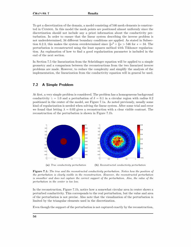
Chapter 7 Results

To get a discretization of the domain, a model consisting of 546 mesh elements is construc-ted in Comsol. In this model the mesh points are positioned almost uniformly since thediscretization should not include any a priori information about the conductivity per-turbation. In order to ensure that the linear system describing the inverse problem isnot underdetermined, 34 different boundary conditions are applied. As stated in Subsec-tion 6.2.3, this makes the system overdetermined since 1

2s2 + 1

2s > 546 for s = 34. Theperturbation is reconstructed using the least squares method with Tikhonov regulariza-tion. An explanation of how to find a good regularization parameter is included in theend of the next section.

In Section 7.5 the linearization from the Schrodinger equation will be applied to a simplegeometry and a comparison between the reconstructions from the two linearized inverseproblems are made. However, to reduce the complexity and simplify the analysis of theimplementation, the linearization from the conductivity equation will in general be used.

7.2 A Simple Problem

At first, a very simple problem is considered. The problem has a homogeneous backgroundconductivity γ = 1.0 and a perturbation of δ = 0.1 in a circular region with radius 0.2positioned in the center of the model, see Figure 7.1a. As noted previously, usually somekind of regularization is needed when solving the linear system. After some trial and errorwe found that letting λ = 0.03 gives a reconstruction with a clear visible contrast. Thereconstruction of the perturbation is shown in Figure 7.1b.

−1 −0.5 0 0.5 1−1

−0.8

−0.6

−0.4

−0.2

0

0.2

0.4

0.6

0.8

1

0.01

0.02

0.03

0.04

0.05

0.06

0.07

0.08

0.09

0.1

(a) True conductivity perturbation

−1 −0.5 0 0.5 1−1

−0.8

−0.6

−0.4

−0.2

0

0.2

0.4

0.6

0.8

1

−0.01

0

0.01

0.02

0.03

0.04

0.05

0.06

(b) Reconstructed conductivity perturbation

Figure 7.1: The true and the reconstructed conductivity perturbation. Notice how the position ofthe perturbation is clearly visible in the reconstruction. However, the reconstructed perturbationis smoother and does not capture the correct support of the perturbation. Also, the value of theperturbation in the center is too low.

In the reconstruction, Figure 7.1b, notice how a somewhat circular area in center shows aperturbed conductivity. This corresponds to the real perturbation, but the value and areaof the perturbation is not precise. Also note that the visualization of the perturbation islimited by the triangular elements used in the discretization.

Even though the support of the perturbation is not captured exactly by the reconstruction,

56

Position of the Perturbation Section 7.3the position and approximate size of the perturbation is clearly visible and in many casesthis will be sufficient to make conclusions about the interior of some medium. The meshis not rotational symmetric, which probably is the reason why neither the reconstructionis symmetric. Also note how we get some small values in a ring shape near the boundary.This is of course an error and if the numeric value of the perturbation is approximatelyknown such errors could easily be removed by choosing a threshold value. This wouldmean that all reconstructed values below the threshold value would be interpreted asbeing zero.

The reconstruction is very dependent of the regularization parameter. Also, the ”best”regularization parameter is very dependent on the problem in question. If the value ofthe Tikhonov parameter is too small the reconstruction is dominated by numerical errors.On the other hand, if it is too large the penalty for large terms makes the value of thereconstructed perturbation approach zero. To find a good Tikhonov paramater, start witha small value. At this point the reconstruction would include a lot of noise. The parameteris then increased until the reconstruction shows areas of nearly zero perturbation repre-senting the background conductivity. At the same time the perturbation should appear,hopefully with a clear contrast. Proceeding with a larger parameter would make the valueof the perturbation smaller and the area of perturbation becomes larger. An example ofa too small and too large regularization parameter can be seen in Figure 7.2.

−1 −0.5 0 0.5 1−1

−0.8

−0.6

−0.4

−0.2

0

0.2

0.4

0.6

0.8

1

−0.2

−0.15

−0.1

−0.05

0

0.05

0.1

0.15

0.2

0.25

(a) Tikhonov regularization parameter λ =0.003

−1 −0.5 0 0.5 1−1

−0.8

−0.6

−0.4

−0.2

0

0.2

0.4

0.6

0.8

1

0

2

4

6

8

10

x 10−3

(b) Tikhonov regularization parameter λ = 0.3

Figure 7.2: An example of how to find a good value of the regularization parameter. To the leftthe value of the parameter is too small and the reconstruction is dominated by noise. To the rightthe value is too large, resulting in a large perturbation area with too small perturbation values.

7.3 Position of the Perturbation

To determine if the algorithm is able to localize a perturbation which is not necessarilycentred, the circular perturbation is moved away from the center, such that it now hasits center at the point (0.4, 0.4), see Figure 7.3a. In this setting it will also be possibleto detect any angular errors which are not visible in the previous reconstruction becauseof the rotational symmetry. Again a regularization parameter of λ = 0.03 gives a goodreconstruction. The result is shown in Figure 7.3b. Looking at the reconstruction, themethod clearly gives the right location of the perturbation. Taking into account that the

57

Chapter 7 Results

−1 −0.5 0 0.5 1−1

−0.8

−0.6

−0.4

−0.2

0

0.2

0.4

0.6

0.8

1

0.01

0.02

0.03

0.04

0.05

0.06

0.07

0.08

0.09

0.1

(a) True conductivity perturbation

−1 −0.5 0 0.5 1−1

−0.8

−0.6

−0.4

−0.2

0

0.2

0.4

0.6

0.8

1

0

0.02

0.04

0.06

0.08

0.1

0.12

(b) Reconstructed conductivity perturbation

Figure 7.3: The position of the perturbation is captured by the reconstruction, but the value andsupport is not correct.

perturbation is only represented by about a dozen of elements due to the discretization,the value and area are also captured very well. In the rotational symmetric case thereconstruction included a ring shaped error near the boundary, but in this reconstructionnothing similar is visible. Thus, the error was probably due to the symmetry of theprevious model, which caused some kind of ”error resonance” significantly increasing theeffect of small errors.

7.4 Effect of Noise

In real-life applications the data originates frommeasurements carried out using electrodespositioned on the exterior of some object. As a result, the measurements are often affectedby noise. For the method to be useful in these kinds of more realistic applications, it isimportant that the method and the corresponding algorithm are still able to reconstructthe perturbation.

Assume that the current measurements are unaffected by noise or assume that the nu-merical errors are neglectable. Then artificial noise can be added to each measurement.For a complex measurement m, the noise is defined as a random complex point uniformlydistributed inside a unit circle of radius |m| · F around the measurement. Here |m| de-notes the complex modulus of m and F is the noise factor. The noise factor F controlsthe percentage of noise added to the measurement. For example, using F = 0.01 wouldgive a measurement with 1% noise. Thus, for each measurement m the noise affectedcounterpart m is defined by

m = m+ rand([0, 1]) · |m| · F · exp (i · rand([−π, π[)) ,

where rand([a, b]) is a random number in the interval [a, b]. Note that this noise onlyaffects the right-hand side of the linear system. The matrixA is assumed to be determinedwithout errors.

The procedure explained above is now used to add noise to the measurements from themodel presented in the previous section. Without any knowledge of the amount noise in

58

Effect of Noise Section 7.4real-life applications, it is assumed that the measurements are fairly precise. As a roughestimate, 5%, 10% and 15% noise is added to the measurements. Three reconstructionsusing the same Tikhonov parameter as before (λ = 0.03), is depicted to the left in Fi-gure 7.4.

It is clear that the method is very sensitive to noise in the measurements. Looking at thereconstruction, it is not possible to conclude anything about the position or the value ofthe perturbation. Actually, it is difficult to even conclude that there is a perturbation.

By changing the Tikhonov parameter, it is possible to obtain a somewhat homogeneousconductivity distribution with a perturbation in the top right corner in all three case.The results are shown to the right in Figure 7.4. For all three reconstructions, the Ti-khonov parameter had to be be increased. This makes sense, since increasing the penaltyfor large values reduces the impact from the noise. The cost is that the correct values inthe reconstruction also gets smaller, which makes the contrast between the backgroundconductivity and the perturbation less noticeable. However, in all three cases it is stillpossible to determine the approximate location and area of the perturbation if the regu-larization parameter is chosen wisely. But, of course one should always try to eliminateall sources of noise as noise always will make the reconstruction less precise.

59

Chapter 7 Results

−1 −0.5 0 0.5 1−1

−0.8

−0.6

−0.4

−0.2

0

0.2

0.4

0.6

0.8

1

−0.6

−0.4

−0.2

0

0.2

0.4

0.6

(a) Reconstruction with Tikhonov regulariza-tion (λ = 0.03). 5% noise.

−1 −0.5 0 0.5 1−1

−0.8

−0.6

−0.4

−0.2

0

0.2

0.4

0.6

0.8

1

−0.02

−0.01

0

0.01

0.02

0.03

0.04

0.05

0.06

(b) Reconstruction with Tikhonov regulariza-tion (λ = 0.1). 5% noise.

−1 −0.5 0 0.5 1−1

−0.8

−0.6

−0.4

−0.2

0

0.2

0.4

0.6

0.8

1

−1.5

−1

−0.5

0

0.5

1

(c) Reconstruction with Tikhonov regulariza-tion (λ = 0.03). 10% noise.

−1 −0.5 0 0.5 1−1

−0.8

−0.6

−0.4

−0.2

0

0.2

0.4

0.6

0.8

1

−0.01

0

0.01

0.02

0.03

0.04

(d) Reconstruction with Tikhonov regulariza-tion (λ = 0.2). 10% noise.

−1 −0.5 0 0.5 1−1

−0.8

−0.6

−0.4

−0.2

0

0.2

0.4

0.6

0.8

1

−2

−1.5

−1

−0.5

0

0.5

1

1.5

2

(e) Reconstruction with Tikhonov regulariza-tion (λ = 0.03). 15% noise.

−1 −0.5 0 0.5 1−1

−0.8

−0.6

−0.4

−0.2

0

0.2

0.4

0.6

0.8

1

−0.02

−0.01

0

0.01

0.02

0.03

0.04

(f) Reconstruction with Tikhonov regulariza-tion (λ = 0.25). 15% noise.

Figure 7.4: Having noisy measurements, the reconstruction is very dependent on regulariza-tion. Using a regularization parameter not adjusted according to the level of noise makes thereconstruction poor. The value has to be increased such that we are able to get a decent pictureshowing the perturbation in the top right corner. Not surprisingly, more noise makes makes thereconstruction less precise. Also the value of the perturbation is reduced when the parameter isincreased.

60

Reconstruction Using the Schrodinger Linearization Section 7.57.5 Reconstruction Using the Schrodinger Linearization

The reconstruction procedure is not limited to the classical linearization method. Asstated previously, the reconstruction algorithm can easily be modified to work with thelinearization from the Schrodinger equation. To match the Schrodinger linearization, thealgorithm must import the value of the potentials instead of the gradients from Comsol

and the solution to the linear system is then a reconstruction of the Schrodinger potential.Remember that the Schrodinger linearization requires that the conductivity γ is twicecontinuously differentiable. To comply with this, a step function with a smooth transitionzone of 0.01 is used to make the perturbation as described in Section 6.4.

Again the model from Section 7.3 is considered. Following the definition of q, it is expectedthat q would behave like the Laplacian of γ, i.e. it should be zero in areas away from theperturbation and have a smooth behaviour in areas where the potential changes. Thus, tofind a good Tikhonov parameter we seek a reconstruction which has these characteristics.Even though the properties of the perturbation is unknown, it is still possible to look forthese characteristics. This is because the reconstruction is expected to have one or a fewperturbations positioned in a homogeneous background conductivity, which covers mostof the domain.

A value of λ = 0.01 was found to give a good reconstruction. An example of a reconstruc-tion of the potential using three different values of λ is shown in Figure 7.5. Note thatthese figures show the reconstructed potential and not the reconstructed conductivity.

−1 −0.5 0 0.5 1−1

−0.8

−0.6

−0.4

−0.2

0

0.2

0.4

0.6

0.8

1

−10

−5

0

5

10

(a) Reconstruction of the po-tential using λ = 0.001

−1 −0.5 0 0.5 1−1

−0.8

−0.6

−0.4

−0.2

0

0.2

0.4

0.6

0.8

1

−3

−2.5

−2

−1.5

−1

−0.5

0

0.5

1

1.5

(b) Reconstruction of the po-tential using λ = 0.01

−1 −0.5 0 0.5 1−1

−0.8

−0.6

−0.4

−0.2

0

0.2

0.4

0.6

0.8

1

−0.1

−0.05

0

0.05

0.1

0.15

0.2

0.25

(c) Reconstruction of the po-tential using λ = 0.1

Figure 7.5: The reconstruction of the potential using different regularization parameters. Agood value gives a reconstruction which are nearly zero in areas away from the perturbation andsmooth in areas where the perturbation changes. A value of λ = 0.01 seems to give a reconstructedpotential with the expected characteristics.

As stated in Theorem 4.3, the conductivity can uniquely be determined from the potentialby solving a simple 2D PDE. This is done numerically in Comsol, using the boundarycondition γ|∂U = 1, as explained in Section 6.4. The result is shown in Figure 7.6b.To make the comparison of the two reconstruction methods simple, the correspondingreconstruction using the classical linearization is depicted in Figure 7.6a.� Remark Note that Figure 7.6b is an image of the conductivity per-

turbation found by solving a PDE in Comsol. The visualization of theperturbation is not limited to the discrete elements that represents the re-constructed potential. As a result, the discretization and the mesh is not

61

Chapter 7 Results

−1 −0.5 0 0.5 1−1

−0.8

−0.6

−0.4

−0.2

0

0.2

0.4

0.6

0.8

1

0

0.02

0.04

0.06

0.08

0.1

0.12

(a) Reconstruction of the conductivity pertur-bation using the classical linearization

(b) Reconstruction of the conductivity usingthe Schrodinger linearization

Figure 7.6: To the right is the reconstruction of the conductivity perturbation using the Schrodin-ger linearization. The reconstruction of the same problem using the classical linearization is sho-wed to the left.

visible in the figure and it may trick the brain to prefer this solution simplybecause of its smooth nature. Keep this in mind when comparing the twoimages.

The Schrodinger linearization gives a reconstruction with a correct position of the pertur-bation. Also the center of the reconstructed perturbation attains a value that is very closeto the correct value of δ = 0.1. The shape of the perturbation is difficult to determinedue to the smoothness of the solution. Also the ”direction” of the smoothing seems to betowards the center of the domain.

The two reconstructions are quite similar in the sense that Figure 7.6b looks as a smoothversion of Figure 7.6a. They are also comparable in the sense that they produce thecorrect value and position with the reconstruction. However, the smoothness of the so-lution from the Schrodinger reconstruction makes it difficult to determine the shape ofthe perturbation. It also includes an extra step in the reconstruction process comparedto the classical linearization reconstruction. As a result, the next section will continue toconsider the linearization from the conductivity equation.

7.6 Multiple Perturbations

So far the classical linearization method has only been tested on problems having a singleperturbation. However, from a theoretical perspective the method is totally capable ofreconstructing a conductivity consisting of multiple separated perturbations. To examinehow well the method handles multiple perturbations, a new problem is now defined. Itincludes a conductivity that is perturbed in three different areas. These areas are a circleto the right, an ellipse at the top left and an ellipse at the bottom left, see Figure 7.7a.In these areas the conductivity is defined as 2.3, 2.0 and 1.3 respectively.

The reconstruction algorithm with homogeneous background conductivity of γ = 1.0 anda regularization parameter of λ = 0.1 produces the reconstruction shown in Figure 7.7b.

62

Non-homogeneous Background Conductivity Section 7.7−1 −0.5 0 0.5 1

−1

−0.8

−0.6

−0.4

−0.2

0

0.2

0.4

0.6

0.8

1

1

1.5

2

2.5

(a) Background conductivity distribution

−1 −0.5 0 0.5 1−1

−0.8

−0.6

−0.4

−0.2

0

0.2

0.4

0.6

0.8

1

−1

−0.8

−0.6

−0.4

−0.2

0

0.2

0.4

0.6

0.8

1

(b) Reconstruction using a homogeneous back-ground conductivity

Figure 7.7: The perturbation now consists of three different areas. The circle to the right, theellipse at the top left and the ellipse at the bottom left has a conductivity of 2.3, 2.0 and 1.3respectively.

Since there is a large difference in conductivity between the different perturbation, theshape of the ellipse at the bottom left is not clearly visible. However, the value of theperturbation in this area is around 0.4 which is close to the correct value. The other twoperturbations are more visible since the value of the perturbation is higher. The valueof the top left perturbation is in agreement with the real perturbation value of 1.0, butthe area is a bit too small. The value of the circular perturbation to the right is alsotoo small. This might be a result of the small area of the circle which makes it morevulnerable to the smoothing, which properly is the due to the discretization being toocoarse in this area. Also note the two dark blue areas near the center which incorrectlylooks as perturbations.

From the previous analysis it can be concluded that a big difference in the size of theperturbation makes it difficult to capture the areas where the perturbation is small. Anya priori information about the approximate value of the perturbations would make itpossible to change the background conductivity such that the magnitudes of the pertur-bations were comparable, since the perturbation is only defined relative to the backgroundconductivity. Also from a theoretical perspective, we want the perturbations to be as smallas possible since we are using a linearization to make the reconstruction. In could there-fore be interesting to see if a non-homogeneous background conductivity could improvethe reconstruction.

7.7 Non-homogeneous Background Conductivity

In many practical applications the perturbation is defined in a medium of non-homogeneousbackground conductivity. An example is a setup where the medical state of some organis tested using EIT by positioning electrodes on surface around the organ and comparethe reconstructed conductivity to a background conductivity. The background conducti-vity would then be the non-homogeneous conductivity distribution around the organ ina healthy human. It is therefore interesting to test if the reconstruction benefits from alinearization around a non-homogeneous background conductivity in these kinds of situa-

63

Chapter 7 Results

tions.

The reconstruction is expected to be more precise if the linearization is made around abackground conductivity closer to the correct conductivity. This could produce smallerrelative perturbations and the theory is made entirely on the assumption of small per-turbations. Also in the case of multiple perturbations, one could choose a backgroundconductivity such that the values of the perturbations were more equal and it would bemore easy identify the shape in the reconstruction.

The mathematical derivation of the reconstruction using the linearization from the conduc-tivity equation is considering a homogeneous background conductivity. Thus, it has notbeen proved that the NtD map uniquely determines the conductivity perturbation if thelinearization is made around a non-homogeneous background conductivity in R2. How-ever, it might be possible that the method still gives usable results in this case. This willbe examined in the following where both single and multiple perturbations are treated.

7.7.1 A Single Perturbation

Consider the problem from Section 7.3 consisting of a single circular perturbation posi-tioned in a unit disc having conductivity γ = 1.0. Now, let the circular perturbation beδ = 0.8. Using a homogeneous background conductivity, the perturbation is reconstructedas depicted in Figure 7.8a. Since the magnitude of perturbation is now large, the penaltyfor large terms had to be reduced. This is reflected in the regularization parameter, whichhad to be lowered to λ = 0.03.

Now assume that some a priori information about the magnitude of the perturbationis available. In real-life situations this could happen if the size and position of someobject is known, but the exact composition of the object is only known approximately.In other words, the shape of the perturbation is known, but the exact value is onlyknown approximately. In this case, a non-homogeneous background conductivity couldbe used instead of a homogeneous background conductivity to make the linearization. Asan example, assume that the expected total conductivity of the perturbed area is γ = 2.0.A regularization parameter of λ = 0.03 gives the reconstruction presented in Figure 7.8b.

Both reconstructions are in great agreement with the real perturbations. The localizationand the area of the perturbation and the value of the relative perturbation is close to thecorrect value in the center of the perturbation. However, when using the non-homogeneousbackground conductivity the relative perturbation becomes smaller and the exact valueof the perturbation is determined with a better precision.

It can be concluded that if the exact shape of the perturbation is known, a non-homogeneousbackground conductivity could give a value of perturbation with better precision. A pro-blem where the exact shape of the perturbation is unknown will be treated in Section 7.8.

7.7.2 Multiple Perturbations

The problem with multiple perturbations is now considered. The non-homogeneous back-ground conductivity consists of three objects positioned in a unit disc having conductivity

64

Non-homogeneous Background Conductivity Section 7.7−1 −0.5 0 0.5 1

−1

−0.8

−0.6

−0.4

−0.2

0

0.2

0.4

0.6

0.8

1

0

0.1

0.2

0.3

0.4

0.5

0.6

0.7

(a) Reconstruction of the perturbation using ahomogeneous background conductivity.

−1 −0.5 0 0.5 1−1

−0.8

−0.6

−0.4

−0.2

0

0.2

0.4

0.6

0.8

1

−0.15

−0.1

−0.05

0

(b) Reconstruction of the perturbation using anon-homogeneous background conductivity.

Figure 7.8: Reconstructions using different background conductivities. Both reconstructions arein great agreement with the real perturbation, but using the non-homogeneous background conduc-tivity the relative perturbation becomes smaller. This means that the value of the perturbation isdetermined with better precision.

γ = 1.0. The circle to the right, the ellipse at the top left and the ellipse at the bottomleft are expected to have a conductivity of 2.5, 1.9 and 1.4 respectively. In these areasthe real conductivity is perturbed relatively by -0.2, 0.1 and -0.1 such that the real totalconductivity is 2.3, 2.0 and 1.3 respectively, see Figure 7.9.

−1 −0.5 0 0.5 1−1

−0.8

−0.6

−0.4

−0.2

0

0.2

0.4

0.6

0.8

1

1

1.5

2

2.5

(a) Background conductivity distribution

−1 −0.5 0 0.5 1−1

−0.8

−0.6

−0.4

−0.2

0

0.2

0.4

0.6

0.8

1

1

1.5

2

2.5

(b) Real conductivity distribution

Figure 7.9: The background conductivity distribution is now non-homogeneous. It consists ofthree objects positioned in a background conductivity of γ = 1.0. The circle to the right, the ellipseat the top left and the ellipse at the bottom left have a conductivity of 2.5, 1.9 and 1.4 respectively.The real situation is depicted to the right where the conductivity is 2.3, 2.0 and 1.3 respectively.

The problem is solved using the background conductivity from Figure 7.9a. It turns outthat a regularization parameter of λ = 0.1 gives a decent reconstruction. This is shownin Figure 7.10b.

Comparing this to the reconstruction done with homogeneous background conductivity,Figure 7.10a, the perturbation to the bottom left is more visible. The two other pertur-bations are also visible, with the area of the upper ellipse being larger than before. Allreconstructed perturbations also attains values that are in great agreement with the real

65

Chapter 7 Results

−1 −0.5 0 0.5 1−1

−0.8

−0.6

−0.4

−0.2

0

0.2

0.4

0.6

0.8

1

−1

−0.8

−0.6

−0.4

−0.2

0

0.2

0.4

0.6

0.8

1

(a) Reconstruction using a homogeneous back-ground conductivity

−1 −0.5 0 0.5 1−1

−0.8

−0.6

−0.4

−0.2

0

0.2

0.4

0.6

0.8

1

−0.2

−0.15

−0.1

−0.05

0

0.05

0.1

(b) Reconstruction using a non-homogeneousbackground conductivity

Figure 7.10: The influence from the background conductivity is dependent on the reconstruction.The value and the area of the reconstructed perturbations are more correct if the linearization ismade on a background conductivity making the perturbations relatively smaller.

perturbations.

Using a homogeneous background conductivity, it is difficult to capture a small per-turbation if there exist larger perturbations in the same medium. When using a non-homogeneous background conductivity the relative size of the perturbations become moresimilar and they are more easy to separate from the background conductivity in the vi-sualization.

One other thing to note is that the dark blue areas from Figure 7.10a, that incorrectly looklike perturbations, changes sign when the non-homogeneous linearization is used. As thebackground conductivity is only increased in the non-homogeneous case, one would notexpect the perturbation in these areas to be larger. Comparing the two reconstructions,the conductivity in these areas does not react as expected to the changed backgroundconductivity and in some cases this might be sufficient to conclude that they are notperturbations, but errors in the reconstruction.

From a theoretical point of view, the linearization is only limited to small perturbations.Also if the medium consists of materials with conductivity of very different magnitude,a linearization around a homogeneous conductivity would also result in a reconstructionwith perturbations of very different magnitude. Any small perturbation would be verydifficult to detect and, as noted before, the approximation errors would be larger. Itis therefore always a good idea to use any a priori information to make a backgroundconductivity which makes the perturbations as small as possible, if the exact shapes ofthe perturbations are known.

7.8 Non-homogeneous Background Conductivity with Wrong Shape

So far the exact shape of the perturbation has been known in advance. Very often theexact shapes of the perturbations are unknown and one have only knowledge of theapproximate shape and position. Also in some situations the problem is dynamical such

66

Non-homogeneous Background Conductivity with Wrong ShapeSection 7.8that the area/volume of the perturbation changes in time. This can be the case if one wantsto monitor the function of the lungs or the heart. In this last case, the area (or volume in3D) of the perturbation would change repeatedly during each heart beat, because of thecontraction of the heart. In such cases one would have to assign an approximate shape ofthe perturbation in the background conductivity.

This section will consider a problem where the shape of the perturbation is not consistentwith the shape of the approximated perturbation in the background conductivity. Again,the cases of a single and multiple perturbations are treated.

7.8.1 A Single Perturbation

A problem of non-homogeneous background conductivity is now considered. The perturba-tion of δ = 0.8 is still limited to a circular region, see Figure 7.11b. Now, the linearizationis done around a background conductivity where a perturbation of δ = 0.1 incorrectlyhaving the shape of a square, see Figure 7.11a.

−1 −0.5 0 0.5 1−1

−0.8

−0.6

−0.4

−0.2

0

0.2

0.4

0.6

0.8

1

1

1.1

1.2

1.3

1.4

1.5

1.6

1.7

1.8

1.9

2

(a) The non-homogeneous background conduc-tivity with a wrong shape.

−1 −0.5 0 0.5 1−1

−0.8

−0.6

−0.4

−0.2

0

0.2

0.4

0.6

0.8

1

1

1.1

1.2

1.3

1.4

1.5

1.6

1.7

1.8

1.9

2

(b) The real conductivity distribution having acircular perturbation.

Figure 7.11: The background conductivity now has a square representing the expected perturba-tion. However, the real perturbation is a circular region, meaning that the shape of the perturbationis incorrect in the background conductivity.

Since the shape of the perturbation is incorrect in the background conductivity, the re-lative perturbation is large in the areas that are covered only by the square in the back-ground conductivity and not by the circle in the real perturbation. To remove the influencefrom these large terms, a larger Tikhonov parameter of λ = 0.1 must be used to get thesomewhat clear contrast in the reconstruction. The reconstruction presented in the Sec-tion 7.7.1 should work as a reference. Therefore it is depicted again in Figure 7.12a. Thereconstruction done using a non-homogeneous background conductivity with a wrongshape is depicted in Figure 7.12b.

Comparing the two reconstructions, it is clear that the shape of the inclusion in thebackground conductivity has a big influence on the solution. Using the wrong shape,the perturbation is still visible and approximately the correct value of the perturbationis attained in the center of the reconstructed perturbation. However, the shape is notcaptured very well. In this case it would be better to use a homogeneous background

67

Chapter 7 Results

−1 −0.5 0 0.5 1−1

−0.8

−0.6

−0.4

−0.2

0

0.2

0.4

0.6

0.8

1

−0.15

−0.1

−0.05

0

(a) Reconstruction using a non-homogeneousbackground conductivity with the correct shape.

−1 −0.5 0 0.5 1−1

−0.8

−0.6

−0.4

−0.2

0

0.2

0.4

0.6

0.8

1

−0.3

−0.25

−0.2

−0.15

−0.1

−0.05

0

0.05

(b) Reconstruction using a non-homogeneousbackground conductivity with a wrong shape.

Figure 7.12: The reconstruction is very dependent on the defined shape in the backgroundconductivity. If the shape is wrong the reconstruction suffers from errors which especially makesit difficult to identify the shape of the perturbation.

conductivity giving the reconstruction depicted in Figure 7.8a. This captures the shapeof the perturbation much better.

Comparing the reconstructions in Figure 7.12a, Figure 7.12b and Figure 7.8a it can beconcluded that a non-homogeneous background conductivity should only be used if theexact shape of the perturbation is known. In other cases it is better to use a homogeneousbackground conductivity.

7.8.2 Multiple Perturbations

If the shapes of several perturbations are unknown, the background conductivity mightbe chosen as depicted in Figure 7.13a. Here the perturbations are approximated by rec-tangular regions. The value of the perturbations are expected to be 2.5 in the square and1.9 in the rectangle at the top left and 1.4 in the rectangle at the bottom left. The realconductivity distribution consists of perturbations having circular and elliptic shapes. Inthese areas the real conductivity is perturbed relatively by -0.2, 0.1 and -0.1 such thatthe real total conductivity is 2.3, 2.0 and 1.3 respectively, see Figure 7.13b.

As concluded in the previous section, the reconstruction is much less precise if the back-ground conductivity has an inclusion with a shape different from the real perturbation.In this case it should be even worse as all three perturbations are approximated by wrongshapes. Several different Tikhonov parameters have been tried in the reconstruction pro-cess. In all cases it is not possible to conclude anything from the reconstructions. Examplesof the reconstructions are depicted in Figure 7.14 where three different Tikhonov para-meters have been used.

Again the conclusion would be that a non-homogeneous background conductivity shouldonly be used if the exact shape of the perturbation is known. In situations where multipleperturbations exist, the reconstruction gives no information if the expected shape ofthe perturbation is not correct. In this case one should use a homogeneous backgroundconductivity which gives a decent reconstruction as depicted in Figure 7.10a.

68

Non-homogeneous Background Conductivity with Wrong ShapeSection 7.8

−1 −0.5 0 0.5 1−1

−0.8

−0.6

−0.4

−0.2

0

0.2

0.4

0.6

0.8

1

1

1.5

2

2.5

(a) Non-homogeneous background conductivitydistribution with wrong shape.

−1 −0.5 0 0.5 1−1

−0.8

−0.6

−0.4

−0.2

0

0.2

0.4

0.6

0.8

1

1

1.5

2

2.5

(b) Real conductivity distribution.

Figure 7.13: The background conductivity expects the perturbations to be of rectangular shape.However, the real perturbation consists of a circle and two ellipses.

−1 −0.5 0 0.5 1−1

−0.8

−0.6

−0.4

−0.2

0

0.2

0.4

0.6

0.8

1

−1

−0.5

0

0.5

(a) Reconstruction using anon-homogeneous backgroundconductivity with a wrongshape. λ = 0.03.

−1 −0.5 0 0.5 1−1

−0.8

−0.6

−0.4

−0.2

0

0.2

0.4

0.6

0.8

1

−0.5

−0.4

−0.3

−0.2

−0.1

0

0.1

0.2

(b) Reconstruction using anon-homogeneous backgroundconductivity with a wrongshape. λ = 0.1.

−1 −0.5 0 0.5 1−1

−0.8

−0.6

−0.4

−0.2

0

0.2

0.4

0.6

0.8

1

−0.18

−0.16

−0.14

−0.12

−0.1

−0.08

−0.06

−0.04

−0.02

0

0.02

(c) Reconstruction using anon-homogeneous backgroundconductivity with a wrongshape. λ = 0.3.

Figure 7.14: No matter the size of the Tikhonov parameter, it is not possible to make conclusionabout the perturbation by looking a the reconstruction.

69

Discussion and Perspectives

During this thesis, the basic mathematical theory for EIT has been outlined and someimportant theoretical and numerical results have been presented. In this section theseresults will be discussed and the challenges and perspectives for future modelling projectswill be brought up.

Using the linearizations it was possible to state uniqueness results in Rn, n ≥ 2. In thenon-linear case using the Schrodinger framework it was only possible to state uniquenessin Rn, n ≥ 3. The advantage of the linearizations is the simple numerical implementationof the inverse problem. In other cases it is often beneficial to work directly on the non-linear inverse problem. As noted previously, the ∂-methods provide a powerful frameworkfor fast non-linear 2D reconstructions and an extension of these methods to 3D couldgreatly improve the reconstruction of 3D models. This is an interesting topic for furthertheoretical research.

The presented theory builds on some physical assumptions. These assumptions includean isotropic conductivity and neglection of the effect from the electrodes and it is unk-nown how much influence this will have on real-life measurements. From a mathematicalperspective, the formulation was simplified by making a linearization. In spite of that,the previous chapter shows that the method provides a framework for reconstructing thepotential in simple geometries. Yet it is unknown how well the method will work on morecomplex problems.

Depending on the application, a simple reconstruction algorithm may be sufficient to drawconclusions. To examine a structure for internal defects, a contrast in the conductivitycould often be enough to draw a conclusion. However, 2D models are often too simple todescribe a real-life problem and 3D models are needed to make a realistic description ofthe domain in question. An example is medical applications where a very high precisionis necessary and it is clear that the presented reconstructions does not provide this. Insuch a perspective, the results in the previous chapter, work more as a proof-of-conceptof EIT, since the models are very simple compared to real-life applications. Nonetheless,the presented theory and numerical implementation provides a good starting point foranyone interested in doing research in EIT or similar inverse problems.

The modelling has been limited to a very simple model to test the general performance ofthe method and algorithm, and to ensure that the results were not too specific. This alsomeans that the numerical analysis done in Chapter 7 if far from exhaustive. Only the mostrelevant results were presented and there are many aspects of the method and implemen-tation that still needs investigation. The method could be tested on other geometries andalso a more extensive analysis of the reconstructions using the Schrodinger linearization

71

Discussion and Perspective

should be made. This linearization could be very useful on problems where the pertur-bation is known to be smooth. The implementation could also be improved in variousways. The boundary integral is calculated using the trapezoidal rule, which is a simplefirst order integration technique. Higher order methods like Simpson’s rule [53] or themore complex Gaussian quadrature formulas on curves [54] or Monte Carlo integrationon surfaces [55] would improve the accuracy. Also a finer mesh could be used to increasethe resolution of the reconstruction. As boundary conditions, complex exponentials werechosen because they are simple orthogonal functions in L2

�(∂U). Maybe more advancedorthogonal functions like wavelets could be used as boundary conditions instead. Alsorecently it has been proved theoretically that the error caused by neglecting second orderterms in the linearization does not affect the shape of the reconstructed perturbationfor piecewise-analytic conductivities [56]. Therefore it is expected that the shape of thereconstructed perturbations would be more accurate if the discretization was finer.

Other regularization methods should also be considered. As noted in Section 6.3 thereexists more advanced regularization methods like PEPR, which supposedly improves thereconstruction image quality [51]. One could also consider working with some of themore advanced modelling toolboxes suitable for modelling both the forward and inverseproblem. Many are included in the EIDORS software package, which provides a platformfor fast prototyping of different reconstruction schemes in EIT [57]. In this case it wouldbe important to acquaint oneself with the techniques used in the implementation.

The motivation behind this thesis has been the interest of the inverse problem. Muchof this interest is due to the difficulty and the use of abstract functional analysis inthe mathematical treatment. Even though some of the mathematical treatment is a bitcomplex, the derivations have been kept as fairly simple and it made it possible to showEIT working as an imaging technique using a numerical implementation. The successrelies on these simplifications, since a more complicated model would make the theoreticaltreatment too advanced and the numerical implementation too complex, considering thelimited time available for this thesis.

72

Conclusion

In this thesis a thorough mathematical treatment of EIT has been done. Two linearizationsrepresenting the inverse problem have been derived and they have both been implementedand tested numerically.

In the first five chapters, the basic theory for EIT has been outlined and some impor-tant theoretical results have been presented. Existence and uniqueness of solutions to theforward problem were proved and this introduced the reader to some important mathe-matical concepts that were needed throughout the thesis. The most important theoreticalresults are stated in Chapter 3 and Chapter 5 where the two different linearizations arederived along with proofs concerning uniqueness of the conductivity reconstructed fromthe linearized NtD map.

Using the Calderon approach [1], modified to work with the NtD map, the inverse pro-blem was given by a linearization of the quadratic map. It was possible to show that theNtD map linearized around a homogeneous conductivity uniquely determines the pertur-bation in Rn, n ≥ 2. In Chapter 4 the CGO theory was introduced. This made it possibleto show that the original non-linear NtD map uniquely determines the conductivity inRn, n ≥ 3. As a new approach, a linearization of the quadratic form was obtained fromthe Schrodinger equation. In this case it was also possible to prove that the NtD maplinearized around a homogeneous conductivity uniquely determines the perturbation inRn, n ≥ 2.

The two linearized inverse problems were formulated in such way that a simple numeri-cal implementation was possible. Chapter 6 described the implementation of the inverseproblem and the results were shown in Chapter 7. The implementation made it possibleto reconstruct the conductivity perturbation in simple geometries. It was shown that themethod produced a reconstruction with approximately the correct location and value. Themethod was also tested on a non-homogeneous background conductivity, which provedto be advantageous if the exact shapes of the perturbations was known. However, if theshapes of the perturbations were only known approximately, the reconstruction proved tobe better when using a homogeneous background conductivity.

The objectives of this thesis have been achieved. The theoretical derivations providesuseful results and could work as a basis for anyone interested in the theoretical conceptsof EIT and the numerical implementation provides insight to an application of EIT insimple geometries. It was concluded that the presented numerical method is too simpleto work with real-life applications, but together with the presented theory it is a goodstarting point for doing further research in the area of inverse problems.

73

Appendices

Appendix A

A.1 Proof of Theorem 4.1

The generalized Laplace equation is defined by

Lγu = ∇ · γ∇u.

Using the product rule of divergence it can be expresses as

Lγu = ∇γ · ∇u+ γ∆u.

The equation is then multiplied by γ− 12

γ− 12Lγu = γ− 1

2∇γ · ∇u+ γ12∆u.

Note that γ− 12∇γ = 2∇γ

12 . This gives

γ− 12Lγu = 2∇γ

12 · ∇u+ γ

12∆u.

From simple differential calculations it follows that

∇ · ((∇γ12 )u+ γ

12∇u) = (∆γ

12 )u+ 2∇γ

12 · ∇u+ γ

12∆u.

Using this result the equation can be reformulated as

γ− 12Lγu = ∇ · ((∇γ

12 )u+ γ

12∇u)− (∆γ

12 )u

= ∇ · ∇(γ12 u)− (∆γ

12 )u

= ∆(γ12u)− (∆γ

12 )u.

A a new function v = γ12 u i defined. The equation can be expressed in terms of w as

γ− 12Lγ(γ

− 12w) = (∆− q)w,

where q = ∆γ12

γ12. Thus, if u is a solution to Lγu = 0 then

(∆− q)w = 0.

As γ ∈ C2(U), then clearly v = γ12 u ∈ H1(U) as u ∈ H1(U).

75

Appendix AA.2 Proof of Theorem 4.4

We write ζ = s (ω1 + iω2), where s = |ζ|√2and ω1 and ω2 being orthogonal unit vectors in

Rn. By an appropriate rotation of the coordinate system ζ can be expressed in the formζ = s(e1 + ie2), where e1 and e2 denotes the first and second unit vectors. Using thisexpression in (4.5) gives

(∆− 2s(e1 + ie2) · ∇) r = f ⇐⇒(∆− 2s(∇1 + i∇2)) r = f, (1)

where ∇jr denotes the j’th coordinate of the gradient ∇r.

For simplicity, assume that U is contained in the n-dimensional hypercube Q = [−π, π]n.If this is not sufficient, one would consider Q = [−jπ, jπ]n, j ∈ N, j > 1. Extend f to bezero outside U , then

(∆− 2s(∇1 + i∇2)r = f, in Q.

The aim is now to construct an appropriate orthonormal basis in L2(Q). Let wk(x) =exp(i(k+ 1

2e2) ·x) . We claim that {wk}k∈Zn is an orthonormal basis for the space L2(Q)having the inner product

(u, v) =1

(2π)n

∫

Q

uv dx, u, v ∈ L2(Q).

To prove this we first show that {wk}k∈Zn is an orthonormal system. This follows fromthe fact that (wk, wl) = 0 if k 6= l and (wk, wk) = 1. To show that it is an orthonormalbasis for the space L2(Q), it is then enough to show that if v ∈ L2(Q) and (v, wk) = 0for all k ∈ Zn, then v = 0 [26]. In other words show that {wk}k∈Zn is complete in L2(Q).We see that if (v, wk) = 0 for all k ∈ Zn then

(v, wk) = (v, exp(i(k +1

2e2) · x))

= (v exp(−i1

2e2 · x), exp(ik · x)) = 0.

It follows that v exp(−i 12e2 · x) = 0 ⇒ v = 0, thus wk is an orthonormal basis for thespace L2(Q). As {wk}k∈Zn is an orthonormal basis, we can expand f, r ∈ L2(Q) as infiniteseries in the following way [26]

f =∑

k∈Zn

fkwk =∑

k∈Zn

(f, wk)wk,

r =∑

k∈Zn

rkwk =∑

k∈Zn

(r, wk)wk.

Using these expressions in (1) yields

(∆− 2s(∇1 + i∇2)∑

k∈Zn

rkwk =∑

k∈Zn

fkwk ⇐⇒(

−(

k +1

2e2

)2

− 2s

(

k1 + i

(

k2 +1

2

))

)

∑

k∈Zn

rkwk =∑

k∈Zn

fkwk,

76

Appendix Awhere k1 and k2 denotes the first two coordinates of the vector k. Note that

Im

(

−(

k +1

2e2

)2

− 2s

(

k1 + i

(

k2 +1

2

))

)

= −2s

(

k2 +1

2

)

is never zero as k ∈ Zn. Hence, in this case there is no problem dividing by the term infront of

∑

k∈Zn rkwk. It follows that the function r can be expressed as

r =∑

k∈Zn

rkwk,

where the expansion coefficients are given by

rk =fk

−(

k + 12e2)2 − 2s

(

k1 + i(

k2 +12

))

. (2)

This series is converging in L2(Q), since

|rk| ≤|fk|

|(

k + 12e2)2

+ 2s(

k1 + i(

k2 +12

))

|

≤ |fk||2s(

k1 + i(

k2 +12

))

|

≤ |fk||s| . (3)

Hence, the coefficients of r are bounded by the coefficients of f . This also gives an upperbound of the norm of r, as

‖r‖L2(Q) =

(

∑

k

|rk|2)

12

≤ 1

|s|

(

∑

k

|fk|2)

12

=1

|s| ‖f‖L2(Q).

Having s = |ζ|√2yields the following bound

‖r‖L2(Q) ≤√2

|ξ| ‖f‖L2(Q), k ∈ Zn.

We now show the boundedness of ∇r. Using the series above ∇r can be expressed as

∇r =∑

k∈Zn

i

(

k +1

2e2

)

rkwk.

To show that this is a convergent series in L2(Q), it is convenient to show it in twodifferent cases.

If∣

∣i(

k + 12e2)∣

∣ ≤ 4s , using (3) gives

∣

∣

∣

∣

i

(

k +1

2e2

)

rk

∣

∣

∣

∣

≤ 4s |rk| ≤ 4 |fk| , k ∈ Zn.

77

Appendix AOn the other hand, if

∣

∣i(

k + 12e2)∣

∣ ≥ 4s we have the following

∣

∣

∣

∣

∣

(

k +1

2e2

)2

+ 2s

(

k1 + i

(

k2 +1

2

))

∣

∣

∣

∣

∣

≥∣

∣

∣

∣

∣

∣

∣

∣

∣

k +1

2e2

∣

∣

∣

∣

2

+ 2sk1

∣

∣

∣

∣

∣

≥∣

∣

∣

∣

k +1

2e2

∣

∣

∣

∣

2

− 2s

∣

∣

∣

∣

k +1

2e2

∣

∣

∣

∣

≥ 1

2

∣

∣

∣

∣

k +1

2e2

∣

∣

∣

∣

2

,

which using (3) implies

∣

∣

∣

∣

i

(

k +1

2e2

)

rk

∣

∣

∣

∣

≤∣

∣k + 12e2∣

∣

12

∣

∣k + 12e2∣

∣

2 |fk| ≤1

12

∣

∣k + 12e2∣

∣

|fk| ≤1

2s|fk| , k ∈ Z

n.

As s = |ζ|√2≥ 1√

2we have

∣

∣

∣

∣

i

(

k +1

2e2

)

rk

∣

∣

∣

∣

≤ 1√2|fk| , k ∈ Z

n.

Thus, for all s the upper bound on the norm is

‖∇r‖L2(Q) ≤ 4‖f‖L2(Q).

As the estimate in L2(U) is proportional to the estimate in L2(Q) the stated boundsfollows.

78

Appendix AA.3 Proof of Theorem 4.5

Before continuing to the case of non-zero potential in the Schrodinger equation, we definethe solution operator to the problem (4.5) as it simplifies the notation in the followtreatment of the problem.

Definition .1 (The Inverse Operator Gζ)Let ζ ∈ Cn satisfy ζ · ζ = 0 and |ζ| sufficiently large. We denote by Gζ :L2(U) → H1(U) the solution operator

Gζf 7→ r,

where r is the solution to (∆− 2ζ · ∇)r = f .

From Theorem 4.4 we have that that both ‖r‖L2(U) and ‖∇r‖L2(U) are bounded by f

and some constant C. It follows that r ∈ H1(U) and we can make the following boundson ‖Gζ‖,

‖Gζ‖L(L2�(U)) ≤

C

|ζ| and

‖Gζ‖L(L2�(U),H1(U)) ≤ C.

In the case of zero potential, r is given by the solution operator Gζ as

r = Gζf.

Now the potential can be non-zero, and in this case the solution can not be determinedthat easily. Nevertheless, we try to find a solution of the form

r = Gζ f ,

where f ∈ L2(U) is the function we want to find. Using (4.6) we can get the followingequation for f

(∆− 2ζ · ∇+ q)Gζ f = f ⇐⇒(I + qGζ)f = f, in U.

So in order to find f the operator (I + qGζ) must be invertible. We recognize this as aNeumann operator series, it is thus invertible if ‖qGζ‖L(L2

�(U)) < 1 [28]. Using the remark

below the definition of Gζ we have the norm estimate

‖qGζ‖L(L2�(U)) ≤

C

|ζ| ‖q‖L∞(U) .

Thus, the operator is invertible if C|ζ| ‖q‖L∞(U) < 1. If we consider |ζ| ≥ max(2C ‖q‖L∞(U) , 1)

we have that

‖qGζ‖L(L2�(U)) ≤

1

2,

79

Appendix Aand (I + qGζ) is invertible. Thus, f can be expressed as

f = (I + qGζ)−1f.

From the theory of Neumann series, we can write the inverse operator as an infinite series

(I + qGζ)−1 =

∞∑

n=0

(−qGζ)n.

It follows that

∥

∥(I + qGζ)−1∥

∥

L(L2�(U))

=

∥

∥

∥

∥

∥

∞∑

n=0

(−qGζ)n

∥

∥

∥

∥

∥

L(L2�(U))

≤∞∑

n=0

‖qGζ‖nL(L2�(U))

≤∞∑

n=0

(

1

2

)n

= 2.

Thus, ‖f‖L2(U) ≤ 2 ‖f‖L2(U). The desired bounds then follows from Theorem 4.4, byreplacing C by 2C.

80

Appendix BAppendix B

B.1 The NtD Map from a 2D Problem in a Homogeneous Medium

We want to solve Laplace’s equation in a homogeneous medium in a unit disc, see Figure15.

b

γ=1

R=1

Figure 15: The geometry of the problem.

Separation of Variables

From Laplace’s equation in 2D, using separation of variables, we get the product solution

u(r, θ) =

∞∑

n=−∞anr

|n| exp(inθ),

where the term r−|n| has been removed from the radial part as we don’t want a singularityin the center.

Boundary conditions

Now we impose boundary conditions to find an expression for γ ∂u∂ν (1, θ) = g(θ). Zero

integral mean at the boundary gives

∫

δU

u dS = 0 ⇐⇒∫ 2π

0

u(1, θ)dθ = 0 ⇐⇒∫ 2π

0

∞∑

n=−∞an exp(inθ)dθ = 0 ⇐⇒

2πa0 = 0 ⇐⇒a0 = 0

Hence we know the solution will have no constant terms on the boundary.

81

Appendix BThe Neumann Boundary Condition

g(θ) = γ∂u

∂ν(1, θ) ⇐⇒

g(θ) = γ∂u

∂r(1, θ) ⇐⇒

g(θ) =

∞∑

n=−∞γ |n|an exp(inθ)

In this way we see that the coefficients of the expansion of g(θ) can be written in term ofthe coefficients of the solution.

Consider the boundary condition u(1, θ) = f(θ)

f(θ) = u(1, θ) =

∞∑

n=−∞an exp(inθ).

Then we noticed that it is equivalent to having the Neumann condition

g(θ) =∞∑

n=−∞γ |n| an exp(inθ).

To be more general, assume ∂u∂ν (1, θ) = g(θ) has the expansion

g(θ) =

∞∑

n=−∞gn exp(inθ),

with g0 = 0 because we want vanishing integral mean at the boundary. Then this isequivalent to having a Dirichlet problem with boundary value

f(θ) =

∞∑

n=−∞fn exp(inθ)

where

fn =gnγ |n| .

We can now define the Neumann to Dirichlet (NtD) map working on complex exponentialsby

Rγ exp(inθ) =1

γ |n| exp(inθ), n ∈ Z\{0}.

B.2 The NtD Map from a 2D Problem in an Inhomogeneous Medium

We want to solve Laplace’s Equation in an inhomogeneous medium in a unit disc, seeFigure 16. The disc contains two materials having different admittivity, γ. The inner dischas radius s and admittivity γ1 and the outer annulus has inner radius s, outer radiusR = 1 and admittivity γ2.

82

Appendix Bb

γ1

γ2

R=1 s

Figure 16: The geometry of the problem.

Separation of Variables

We denote the solution in the disc region in the center, u1 (as γ = γ1 in this region) andthe solution u2 in the surrounding annulus. From Laplace’s equation in 2D we get theproduct solutions:

u1(r, θ) =∑

n∈Z

an

(r

s

)|n|exp(inθ)

u2(r, θ) = b0 + c0 ln r +∑

n∈Z\{0}[bnr

|n| + cnr−|n|] exp(inθ).

Boundary conditions

Now we impose boundary conditions to find an expression for γ2∂u∂ν (1, θ) = g(θ).

Zero Integral Mean at Boundary

We want zero integral mean at the boundary:

∫

δU

u2 dS = 0 ⇐⇒∫ 2π

0

u2(1, θ) dθ = 0 ⇐⇒∫ 2π

0

b0 +∑

n∈Z\{0}[bn + cn] exp(inθ) dθ = 0 ⇐⇒

2πb0 = 0 ⇐⇒b0 = 0.

Smooth Intersection

At r = s we want a smooth intersection between the two solutions. That is we requirethe function values and the γ-weighted derivatives to be equal.

83

Appendix BEqual function values:

u1(s, θ) = u2(s, θ) ⇐⇒∑

n∈Z

an exp(inθ) = c0 ln s+∑

n∈Z\{0}

[

bns|n| + cns

−|n|]

exp(inθ).

Equal γ-weighted derivatives:

γ1∂u1

∂r(s, θ) = γ2

∂u2

∂r(s, θ) ⇐⇒

γ1∑

n∈Z

|n|san exp(inθ) = γ2

c0s

+ γ2∑

n∈Z\{0}

[

|n| bns|n|−1 − |n| cns−|n|−1]

exp(inθ).

We notice that the last equation implies that c0 = 0. From the two equations we get:

an = bns|n| + cns

−|n|

and

γ1|n|san = γ2

[

|n| bns|n|−1 − |n| cns−|n|−1]

.

Combining the two equations gives

γ1

[

bns|n| + cns

−|n|]

= γ2

[

bns|n| − cns

−|n|]

.

Thus, cn can be expressed as

cn = bnγ2s

|n| − γ1s|n|

γ1s−|n| + γ2s−|n| .

We consider the imposed Neumann boundary condition as a complex Fourier expansion,i.e.

g(θ) =

∞∑

n=−∞gn exp(inθ).

Looking at the partial derivative of the solution and inserting R = 1 we see that

g(θ) = γ2∂u2

∂r(1, θ) =

∑

n∈Z\{0}γ2 [|n| bn − |n| cn] exp(inθ).

It follows that

gn = γ2 |n| [bn − cn] .

Using the found expression for cn, we can express bn in terms of gn:

gn = γ2 |n| [bn − cn] = γ2 |n| bn(

1− γ2s|n| − γ1s

|n|

γ1s−|n| + γ2s−|n|

)

⇐⇒

bn =gn

γ2 |n|(

1− γ2s|n|−γ1s|n|

γ1s−|n|+γ2s−|n|

)

84

Appendix BWe now consider the corresponding Dirichlet boundary condition as a complex Fourierexpansion as well

f(θ) =

∞∑

n=−∞fn exp(inθ).

Looking at the solution we get for the Dirichlet condition:

fn = bn + cn.

Using the found expression for cn we get:

fn = bn

(

1 +γ2s

|n| − γ1s|n|

γ1s−|n| + γ2s−|n|

)

We can now insert the expression for bn to express fn in terms of cn

fn =gn

γ2 |n|1 + γ2s

|n|−γ1s|n|


1− γ2s|n|−γ1s|n|


We define β = γ2−γ1

γ2+γ1 and can thus write

fn =gn

γ2 |n|1 + βs2|n|

1− βs2|n|=

gnγ2 |n|

(

1 +2βs2|n|

1− βs2|n|

)

.

We can now define the Neumann to Dirichlet (NtD) map working on complex exponentialsby

Rγ exp(inθ) =1

γ2 |n|1 + βs2|n|

1− βs2|n|exp(inθ), n ∈ Z\{0}.

85

Appendix CAppendix C

C.1 The Code for Building the Linear System

1 %% Parameters2

3 % Start clock4 tic5

6 % Number of applied boundary condicition7 s = 34;8

9 % Boundary-ids of the model10 boundarynodes = [13 14 15 16];11

12 %% Load mesh model13

14 % Load and solve model once to ensure it is up-to-date15 disp( 'Loading model' )16 model = mphload( 'bgmodel.mph' );17 model.study( 'std1' ).run;18

19 %% Get mesh and geometry data20

21 % Boundary lenght22 bl = mphint(model, '1' , 'edim' ,1, 'Selection' ,[1 2 3 4]);23

24 % Mesh Data25 disp( 'Getting mesh data' );26 mesh = mpheval(model, 'meshelement' , 'Smooth' , 'none' , 'Edim' ,2);27

28 % Number of elements29 N=length(mesh.t);30

31 % Points of element centers P and volume of each element V32 P=zeros(N,2);33 V=zeros(1,N);34 for j=1:N35 tmp = mesh.p(:,find(mesh.d1==j))';36 P(j,:) = sum(tmp)/3;37 V(j) = 1/2 * abs(det([tmp'; 1 1 1]));38 end39

40 %% Load background model41

42 % Load and solve model to ensure it is up-to-date43 model = mphload( 'comsol-model.mph' );44 model.study( 'std1' ).run;45

46 % Set background condictivity in all shapes of the model geom etry47 model.physics( 'c' ).feature( 'cfeq1' ).set( 'c' , { '1' '0' '0' '1' });48 model.physics( 'c' ).feature( 'cfeq2' ).set( 'c' , { '1' '0' '0' '1' });49 model.physics( 'c' ).feature( 'cfeq3' ).set( 'c' , { '1' '0' '0' '1' });50 model.physics( 'c' ).feature( 'cfeq4' ).set( 'c' , { '1' '0' '0' '1' });51

52 % Allocate memory53 UX = zeros(s,N);54 UY = zeros(s,N);55 UXI = zeros(s,N);

86

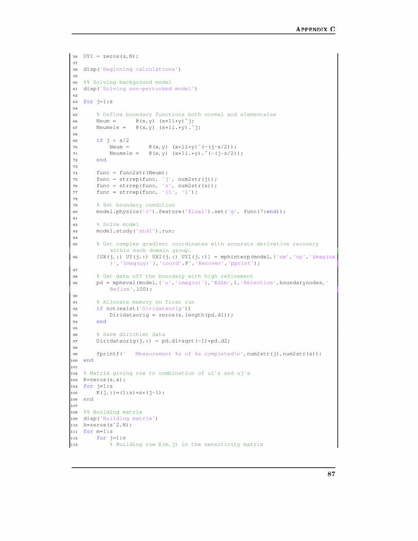
Appendix C56 UYI = zeros(s,N);57

58 disp( 'Beginning calculations' )59

60 %% Solving background model61 disp( 'Solving non-perturbed model' )62

63 for j=1:s64

65 % Define boundary functions both normal and elementwise66 Neum = @(x,y) (x+1i * y)ˆj;67 Neumele = @(x,y) (x+1i. * y).ˆj;68

69 if j > s/270 Neum = @(x,y) (x+1i * y)ˆ(-(j-s/2));71 Neumele = @(x,y) (x+1i. * y).ˆ(-(j-s/2));72 end73

74 func = func2str(Neum);75 func = strrep(func, 'j' , num2str(j));76 func = strrep(func, 's' , num2str(s));77 func = strrep(func, '1i' , 'i' );78

79 % Set boundary condition80 model.physics( 'c' ).feature( 'flux1' ).set( 'g' , func(7: end ));81

82 % Solve model83 model.study( 'std1' ).run;84

85 % Get complex gradient coordinates with accurate derivativ e recoverywithin each domain group.

86 [UX(j,:) UY(j,:) UXI(j,:) UYI(j,:)] = mphinterp(model,{ 'ux' , 'uy' , 'imag(ux)' , 'imag(uy)' }, 'coord' ,P', 'Recover' , 'pprint' );

87

88 % Get data off the boundary with high refinement89 pd = mpheval(model,{ 'u' , 'imag(u)' }, 'Edim' ,1, 'Selection' ,boundarynodes, '

Refine' ,100);90

91 % Allocate memory on first run92 if not(exist( 'Diridataorig' ))93 Diridataorig = zeros(s,length(pd.d1));94 end95

96 % Save dirichlet data97 Diridataorig(j,:) = pd.d1+sqrt(-1) * pd.d2;98

99 fprintf( ' Measurement %s of %s completed\n' ,num2str(j),num2str(s));100 end101

102 % Matrix giving row to combination of ui's and uj's103 K=zeros(s,s);104 for j=1:s105 K(j,:)=(1:s)+s * (j-1);106 end107

108 %% Building matrix109 disp( 'Building matrix' )110 A=zeros(sˆ2,N);111 for m=1:s112 for j=1:s113 % Building row K(m,j) in the sensitivity matrix

87

Appendix C114 A(K(m,j),:)=-V(:). * (transpose((UX(m,:)+sqrt(-1) * UXI(m,:))). * transpose

(conj(UX(j,:)+sqrt(-1) * UXI(j,:)))+transpose((UY(m,:)+sqrt(-1) *UYI(m,:))). * transpose(conj(UY(j,:)+sqrt(-1) * UYI(j,:))));

115 fprintf( ' Row %s of %s completed\n' ,num2str((m-1) * s+j),num2str(sˆ2));

116 end117 end118

119

120 % Allocating memory121 Diridata = zeros(s,length(pd.d1));122 Neumdata = zeros(s,length(pd.d1));123

124 % Apply conductivity perturbatio125 disp( 'Apply conductivity perturbation' );126 model.physics( 'c' ).feature( 'cfeq1' ).set( 'c' , { '1' '0' '0' '1' });127 model.physics( 'c' ).feature( 'cfeq2' ).set( 'c' , { '1.1' '0' '0' '1.1' });128 model.physics( 'c' ).feature( 'cfeq3' ).set( 'c' , { '1.2' '0' '0' '1.2' });129 model.physics( 'c' ).feature( 'cfeq4' ).set( 'c' , { '1.3' '0' '0' '1.3' });130

131 %% Solving perturbed model132 disp( 'Solving perturbed model' )133 for j=1:s134

135 % Define boundary functions both normal and elementwise136 Neum = @(x,y) (x+1i * y)ˆj;137 Neumele = @(x,y,j) (x+1i. * y).ˆj;138

139 if j > s/2140 Neum = @(x,y) (x+1i * y)ˆ(-(j-s/2));141 Neumele = @(x,y,j) (x+1i. * y).ˆ(-(j-s/2));142 end143

144 func = func2str(Neum);145 func = strrep(func, 'j' , num2str(j));146 func = strrep(func, 's' , num2str(s));147 func = strrep(func, '1i' , 'i' );148

149 % Set boundary condition150 model.physics( 'c' ).feature( 'flux1' ).set( 'g' , func(7: end ));151

152 % Solve153 model.study( 'std1' ).run;154

155 % Get data off the boundary with high refinement156 pd2 = mpheval(model,{ 'u' , 'imag(u)' }, 'Edim' ,1, 'Selection' ,boundarynodes, '

Refine' ,100);157

158 % Save Dirichlet data159 Diridata(j,:) = pd2.d1+sqrt(-1) * pd2.d2;160 % Calculate Neumann data161 Neumdata(j,:) = Neumele(pd2.p(1,:),pd2.p(2,:),j);162

163 fprintf( ' Measurement %s of %s completed\n' ,num2str(j),num2str(s));164 end165

166 %% Building right-hand side167 disp( 'Building right-hand side' )168

169 b=zeros(sˆ2,1);170 for m=1:s171 for j=1:s

88

Appendix C172 % Calculate b elements by using the trapezoidal rule.173 b(K(m,j))=(Diridata(m,:)-Diridataorig(m,:)) * transpose(conj(Neumdata(j

,:)))./length(pd2.d1). * bl;174 fprintf( ' Row %s of %s completed\n' ,num2str((m-1) * s+j),num2str(sˆ2)

);175 end176 end177 disp( 'Done' )178 fprintf( 'Elapsed time: %0.0f secs\n' ,toc)179 %Save data for future use180 save([ 'EIT_Meshelelements' ,num2str(N), '_BCs' ,num2str(s)]);

89

Appendix CC.2 The Code for Solving the Linear System

1 %% Tikhonov Regularization2

3 % Set the noisefactor. If Noisefactor=0.0 no noise is added4 Noisefactor=0.0;5

6 % Add noise if Noisefactor>07 if Noisefactor>08 % Calculate new boundary data with added noise9 DiridataNoise = Diridata+abs(Diridata). * Noisefactor. * rand(size(

Diridata)). * exp(i * (-pi+2 * rand(size(Diridata)) * pi));10 DiridataorigNoise = Diridataorig+abs(Diridataorig). * Noisefactor. * rand(

size(Diridataorig)). * exp(i * (-pi+2 * rand(size(Diridataorig)) * pi));11 NeumdataNoise = Neumdata+abs(Neumdata). * Noisefactor. * rand(size(

Neumdata)). * exp(i * (-pi+2 * rand(size(Neumdata)) * pi));12

13 % Rebuild righthand side with the new data14 b=zeros(sˆ2,1);15 for m=1:s16 for j=1:s17 b(K(m,j))=(DiridataNoise(m,:)-DiridataorigNoise(m,: )) * transpose(

conj(NeumdataNoise(j,:)))./length(pd2.d1). * bl;18 end19 end20 end21

22 % Set Tikhonov regularization parameter23 lambda = 0.1;24

25 % Change A and b to include the Tikhonov regularization26 q=length(A(1,:));27 A = [A;lambdaˆ2 * eye(q)];28 b = [b;zeros(q,1)];29

30 % Solving the problem using the least squares method regular ization31 x=A\b;32

33 % Make a plot where each triangular element has the color of th e value in34 % the centroid.35

36 x2=zeros(1,length(mesh.p(1,:)));37 for j=1:N38 tmp = find(mesh.d1==j)';39 x2([tmp]) = x(j);40 end41 trisurf((mesh.t+1)',mesh.p(1,:),mesh.p(2,:),real(x2 ))42 colorbar43 % Rotate to get the 2D picture44 view([0 0 90])

90

List of Symbols

U An open bounded subset of Rn, n ≥ 2.

∂U The (smooth) boundary of U .

L∞ The space of bounded functions.

L∞+ The space of strictly positive bounded functions.

L2�(∂U) The space of L2(∂U) functions integrating to zero along ∂U .

L1loc(U) The space of functions in U which are integrable on any compact subset of U .

γ The electrical admittivity. In the case of isotropy and frequency independencethis is also the electrical conductivity.

H1 The Sobolev space H1.

H2 The Sobolev space H2.

H1� Functions in H1 integrating to zero along ∂U .

H−1 The dual space of H1� .

C The space of continuous functions.

C2 The space of functions that are twice continuous differentiable.

∆ The Laplacian operator, ∆ = ∇ · ∇ = ∇2.

〈·, ·〉 The usual L2(∂U) inner product being anti-linear in the second argument.

‖·‖L(X) The X → X operator norm for bounded linear operators.

‖·‖L(X,Y ) The X → Y operator norm for bounded linear operators.

Re(x) The real part of the complex number x.

x The non-unitary Fourier transform of x.

C The set of complex numbers.

R The set of real numbers.

Z The set of integers.

91

Bibliography

[1] A.P. Calderon. On an inverse boundary value problem. Computational & AppliedMathematics, 25(2-3):133–138, 1980.

[2] R.P. Henderson and J.G. Webster. An impedance camera for spatially specific measu-rements of the thorax. Biomedical Engineering, IEEE Transactions on, (3):250–254,1978.

[3] G. Uhlmann. Visibility and invisibility. ICIAM 07: 6th International Conference onIndustrial and Applied Mathematics, Zurich, Switzerland, 16-20 July 2007: invitedlectures, page 381, 2009.

[4] O. Scherzer. Handbook of mathematical methods in imaging. Springer Verlag, 2010.

[5] R. Kohn and M. Vogelius. Determining conductivity by boundary measurements.Communications on Pure and Applied Mathematics, 37(3):289–298, 1984.

[6] J. Sylvester and G. Uhlmann. A global uniqueness theorem for an inverse boundaryvalue problem. The Annals of Mathematics, 125(1):153–169, 1987.

[7] O.Y. Imanuvilov, G. Uhlmann, and M. Yamamoto. The Calderon problem withpartial data in two dimensions. American Mathematical Society, 23(3):655–691, 2010.

[8] K. Knudsen. The Calderon problem with partial data for less smooth conductivities.Communications in Partial Differential Equations, 31(1-3):57–72, 2006.

[9] C.E. Kenig, J. Sjostrand, and G. Uhlmann. The Calderon problem with partial data.Annals of Mathematics-Second Series, 165(2):567–592, 2007.

[10] K. Knudsen, M. Lassas, J.L. Mueller, and S. Siltanen. Regularized d-bar methodfor the inverse conductivity problem. Inverse Problems and Imaging, 3(4):599–624,2009.

[11] Adrian I. Nachman. Global uniqueness for a two-dimensional inverse boundary valueproblem. The Annals of Mathematics, 143(1):pp. 71–96, 1996.

[12] L. Tartar. An introduction to Sobolev spaces and interpolation spaces. SpringerVerlag, 2007.

[13] L. Borcea. Electrical impedance tomography. Inverse problems, 18:R99–R136, 2002.

[14] D. Holder. Electrical impedance tomography: methods, history, and applications. Tay-lor & Francis, 2005.

93

Bibliography

[15] R.V. Kohn. Identification of an unknown conductivity by means of measurements atthe boundary. 1983.

[16] M. Cheney, D. Isaacson, and J.C. Newell. Electrical impedance tomography. SIAMreview, 41(1):85–101, 1999.

[17] David Isaacson and Margaret Cheney. Effects of measurement precision and finitenumbers of electrodes on linear impedance imaging algorithms. SIAM Journal onApplied Mathematics, 51(6):pp. 1705–1731, 1991.

[18] Erkki Somersalo, Margaret Cheney, and David Isaacson. Existence and uniquenessfor electrode models for electric current computed tomography. SIAM J. Appl. Math.,52:1023–1040, August 1992.

[19] Harry Eckel. Numerical study of an evolutionary algorithm for electrical impedancetomography. Dissertation, University of Gottingen, 2007.

[20] Armin Lechleiter, Nuutti Hyvonen, and Harri Hakula. The Factorization MethodApplied to the Complete Electrode Model of Impedance Tomography. SIAM Journalon Applied Mathematics, 68(4):1097–1121, 2008.

[21] Harri Hakula Nuutti Hyvonen and Sampsa Pursiainen. The Factorization MethodApplied to the Complete Electrode Model of Impedance Tomography. Inverse Pro-blems and Imaging., 1(2):299–317, 2007.

[22] Joseph B. Keller. Inverse Problems. The American Mathematical Monthly., 83:107–118, 1976.

[23] L.C. Evans. Partial Differential Equations (Graduate Studies in Mathematics, V.19). American Mathematical Society, 1998.

[24] W. Han. A posteriori error analysis via duality theory: with applications in modelingand numerical approximations. Springer, 2005.

[25] Petri Ola. Lecture notes: Introduction to electrical impedance tomography. http://mathstat.helsinki.fi/kurssit/imptom/EITluennot.pdf , 2008.

[26] O. Christensen. Functions, Spaces, and Expansions: Mathematical Tools in Physicsand Engineering. Birkhauser, 2010.

[27] C. Grossmann, H.G. Roos, and M. Stynes. Numerical treatment of partial differentialequations. Springer Verlag, 2007.

[28] W Cheney. Analysis for applied mathematics. Springer, 2001.

[29] G. Uhlmann. Electrical impedance tomography and Calderon’s problem. InverseProblems, 25(12):123011, 2009.

[30] D.H. Griffel. Applied functional analysis. Dover publications, 2002.

[31] A. Brown and C.M. Pearcy. An introduction to analysis. Springer, 1995.

[32] K. Morita. Applied Fourier Transform. IOS Press, 1995.

[33] D. Isaacson and E. Isaacson. Comment on Calderon’s paper: ”On an inverse boundaryvalue problem”. Math. Comput, 52:553–9, 1989.

94

http://mathstat.helsinki.fi/kurssit/imptom/EITluennot.pdf

http://mathstat.helsinki.fi/kurssit/imptom/EITluennot.pdf

Bibliography

[34] K. Knudsen, M. Lassas, J.L. Mueller, and S. Siltanen. D-bar method for electricalimpedance tomography with discontinuous conductivities. SIAM Journal on AppliedMathematics, 67(3):893, 2007.

[35] J. Sylvester and G. Uhlmann. A uniqueness theorem for an inverse boundary valueproblem in electrical prospection. Communications on Pure and Applied Mathema-tics, 39(1):91–112, 1986.

[36] J. Sylvester and G. Uhlmann. A global uniqueness theorem for an inverse boundaryvalue problem. The Annals of Mathematics, 125(1):pp. 153–169, 1987.

[37] B.H. Bransden and C.J. Joachain. Quantum mechanics. Prentice Hall, 2000.

[38] H. Gao, H. Zhao, and S. Osher. Quantitative Photoacoustic Tomography. submitted.

[39] Guillaume Bal and Gunther Uhlmann. Inverse diffusion theory of photoacoustics.Inverse Problems, 26(8):085010.

[40] D.H. Sattinger, CA Tracy, and S. Venakides. Inverse scattering and applications.Amer Mathematical Society, 1991.

[41] M. Salo. Lecture notes: Calderon problem. http://www.rni.helsinki.fi/

˜ msa/teaching/calderon/calderon_lectures.pdf , 2008.

[42] P. Hahner. A periodic Faddeev-type solution operator. Journal of Differential Equa-tions, 128(1):300 – 308, 1996.

[43] R.M. Brown and R.H. Torres. Uniqueness in the inverse conductivity problem forconductivities with 3/2 derivatives in Lp, p > 2n. Journal of Fourier Analysis andApplications, 9(6):563–574, 2003.

[44] L. Paivarinta, A. Panchenko, and G. Uhlmann. Complex geometrical optics solutionsfor Lipschitz conductivities. Revista Matematica Iberoamericana, 19(1):57–72, 2003.

[45] G. Uhlmann. Electrical impedance tomography and Calderon’s problem. Inverseproblems, 25:123011, 2009.

[46] D. Pedoe. Geometry, a comprehensive course. Dover Pubns, 1988.

[47] JAC Weideman. Numerical integration of periodic functions: A few examples. TheAmerican mathematical monthly, 109(1):21–36, 2002.

[48] G.K.E. Dietl. Linear estimation and detection in Krylov subspaces, volume 1. Sprin-ger Verlag, 2007.

[49] H.W. Engl, M. Hanke, and A. Neubauer. Regularization of inverse problems. SpringerNetherlands, 1996.

[50] H. Niu, P. Guo, L. Ji, Q. Zhao, and T. Jiang. Improving image quality of diffuseoptical tomography with a projection-error-based adaptive regularization method.Optics express, 16(17):12423–12434, 2008.

[51] T.K. Bera, S.K. Biswas, K. Rajan, and J. Nagaraju. Improving image quality in elec-trical impedance tomography (EIT) using projection error propagation-based regula-rization (PEPR) technique: A simulation study. Journal of Electrical Bioimpedance,2(1):2–12, 2011.

95

http://www.rni.helsinki.fi/~msa/teaching/calderon/calderon_lectures.pdf

http://www.rni.helsinki.fi/~msa/teaching/calderon/calderon_lectures.pdf

Bibliography

[52] S. Lea. Mathematics for physicists. Brooks/Cole-Thomson Learning, 2004.

[53] L. Elden, L. Wittmeyer-Koch, and H.B. Nielsen. Introduction to numerical compu-tation: analysis and MATLAB® illustrations. Studentlitteratur, 2004.

[54] M.S. Gockenbach. Understanding and implementing the finite element method. So-ciety for Industrial and Applied Mathematics, 2006.

[55] Ivan T. Dimov. Monte Carlo methods for applied scientists. World Scientific, 2008.

[56] B. Harrach and J.K. Seo. Exact shape-reconstruction by one-step linearization inelectrical impedance tomography. SIAM Journal on Mathematical Analysis, 42(4),2010.

[57] M. Vauhkonen, W.R.B. Lionheart, L.M. Heikkinen, P.J. Vauhkonen, and J.P. Kaipio.A MATLAB package for the EIDORS project to reconstruct two-dimensional EITimages. Physiological Measurement, 22:107, 2001.

96

Linearization in Electrical Impedance Tomography · Abstract This thesis considers a mathematical...

Documents

Transcript of Linearization in Electrical Impedance Tomography · Abstract This thesis considers a mathematical...