
Image Segmentation Applied to Electrical Impedance Tomography

Inside Out IIMSRI PublicationsVolume 60, 2012
Resistor network approaches to electricalimpedance tomography
LILIANA BORCEA, VLADIMIR DRUSKIN,FERNANDO GUEVARA VASQUEZAND ALEXANDER V. MAMONOV
We review a resistor network approach to the numerical solution of the inverseproblem of electrical impedance tomography (EIT). The networks arise in thecontext of finite volume discretizations of the elliptic equation for the electricpotential, on sparse and adaptively refined grids that we call optimal. Thename refers to the fact that the grids give spectrally accurate approximationsof the Dirichlet to Neumann map, the data in EIT. The fundamental feature ofthe optimal grids in inversion is that they connect the discrete inverse problemfor resistor networks to the continuum EIT problem.
1. Introduction
We consider the inverse problem of electrical impedance tomography (EIT) intwo dimensions [Borcea 2002]. It seeks the scalar valued positive and boundedconductivity �.x/, the coefficient in the elliptic partial differential equation forthe potential u 2H 1.�/,
r � Œ�.x/ru.x/�D 0; x 2�: (1-1)
The domain� is a bounded and simply connected set in R2 with smooth boundaryB. Because all such domains are conformally equivalent by the Riemann mappingtheorem, we assume throughout that � is the unit disk,
�D fx D .r cos �; r sin �/; r 2 Œ0; 1�; � 2 Œ0; 2�/g : (1-2)
The EIT problem is to determine �.x/ from measurements of the Dirichlet toNeumann (DtN) map ƒ� or equivalently, the Neumann to Dirichlet map ƒ|
� .We consider the full boundary setup, with access to the entire boundary, and thepartial measurement setup, where the measurements are confined to an accessiblesubset BA of B, and the remainder BI DB nBA of the boundary is grounded(ujBI
D 0).
55

56 L. BORCEA, V. DRUSKIN, F. GUEVARA VASQUEZ AND A. V. MAMONOV
The DtN mapƒ� WH 1=2.B/!H�1=2.B/ takes arbitrary boundary potentialsuB in the trace space H 1=2.B/ to normal boundary currents
ƒ�uB.x/D �.x/n.x/ � ru.x/; x 2B; (1-3)
where n.x/ is the outer normal at x 2 B and u.x/ solves (1-1) with Dirichletboundary conditions
u.x/D uB.x/; x 2B: (1-4)
Note that ƒ� has a null space consisting of constant potentials and thus, it isinvertible only on a subset J of H�1=2.B/, defined by
JD
�J 2H�1=2.B/ such that
ZB
J.x/ds.x/D 0
�: (1-5)
Its generalized inverse is the NtD mapƒ|� WJ!H 1=2.B/, which takes boundary
currents JB 2 J to boundary potentials
ƒ|�JB.x/D u.x/; x 2B: (1-6)
Here u solves (1-1) with Neumann boundary conditions
�.x/n.x/ � ru.x/D JB.x/; x 2B; (1-7)
and it is defined up to an additive constant, that can be fixed for example bysetting the potential to zero at one boundary point, as if it were connected to theground.
It is known that ƒ� determines uniquely � in the full boundary setup [Astalaet al. 2005]. See also the earlier uniqueness results [Nachman 1996; Brownand Uhlmann 1997] under some smoothness assumptions on � . Uniquenessholds for the partial boundary setup as well, at least for � 2 C 3C�. N�/ and � > 0,[Imanuvilov et al. 2008]. The case of real-analytic or piecewise real-analytic �is resolved in [Druskin 1982; 1985; Kohn and Vogelius 1984; 1985].
However, the problem is exponentially unstable, as shown in [Alessandrini1988; Barceló et al. 2001; Mandache 2001]. Given two sufficiently regularconductivities �1 and �2, the best possible stability estimate is of logarithmictype
k�1� �2kL1.�/ � cˇlog kƒ�1
�ƒ�2kH 1=2.B/;H�1=2.B/
ˇ�˛; (1-8)
with some positive constants c and ˛. This means that if we have noisy measure-ments, we cannot expect the conductivity to be close to the true one uniformlyin �, unless the noise is exponentially small.
In practice the noise plays a role and the inversion can be carried out onlyby imposing some regularization constraints on � . Moreover, we have finitely

RESISTOR NETWORKS FOR ELECTRICAL IMPEDANCE TOMOGRAPHY 57
many measurements of the DtN map and we seek numerical approximations of� with finitely many degrees of freedom (parameters). The stability of theseapproximations depends on the number of parameters and their distribution inthe domain �.
It is shown in [Alessandrini and Vessella 2005] that if � is piecewise constant,with a bounded number of unknown values, then the stability estimates on � areno longer of the form (1-8), but they become of Lipschitz type. However, it isnot really understood how the Lipschitz constant depends on the distribution ofthe unknowns in �. Surely, it must be easier to determine the features of theconductivity near the boundary than deep inside �.
Then, the question is how to parametrize the unknown conductivity in numer-ical inversion so that we can control its stability and we do not need excessiveregularization with artificial penalties that introduce artifacts in the results. Adap-tive parametrizations for EIT have been considered for example in [Isaacson1986; MacMillan et al. 2004] and [Ben Ameur et al. 2002; Ben Ameur andKaltenbacher 2002]. Here we review our inversion approach that is based onresistor networks that arise in finite volume discretizations of (1-1) on sparseand adaptively refined grids which we call optimal. The name refers to the factthat they give spectral accuracy of approximations of ƒ� on finite volume grids.One of their important features is that they are refined near the boundary, wherewe make the measurements, and coarse away from it. Thus they capture theexpected loss of resolution of the numerical approximations of � .
Optimal grids were introduced in [Druskin and Knizhnerman 2000b; 2000a;Ingerman et al. 2000; Asvadurov et al. 2000; 2003] for accurate approximationsof the DtN map in forward problems. Having such approximations is importantfor example in domain decomposition approaches to solving second order partialdifferential equations and systems, because the action of a subdomain can bereplaced by the DtN map on its boundary [Quarteroni and Valli 1999]. In addition,accurate approximations of DtN maps allow truncations of the computationaldomain for solving hyperbolic problems. The studies in [Druskin and Knizhner-man 2000b; 2000a; Ingerman et al. 2000; Asvadurov et al. 2000; 2003] workwith spectral decompositions of the DtN map, and show that by just placing gridpoints optimally in the domain, one can obtain exponential convergence ratesof approximations of the DtN map with second order finite difference schemes.That is to say, although the solution of the forward problem is second orderaccurate inside the computational domain, the DtN map is approximated withspectral accuracy. Problems with piecewise constant and anisotropic coefficientsare considered in [Druskin and Moskow 2002; Asvadurov et al. 2007].
Optimal grids are useful in the context of numerical inversion, because theyresolve the inconsistency that arises from the exponential ill posedness of the

58 L. BORCEA, V. DRUSKIN, F. GUEVARA VASQUEZ AND A. V. MAMONOV
problem and the second order convergence of typical discretization schemesapplied to (1-1), on ad-hoc grids that are usually uniform. The forward problemfor the approximation of the DtN map is the inverse of the EIT problem, soit should converge exponentially. This can be achieved by discretizing on theoptimal grids.
In this article we review the use of optimal grids in inversion, as it wasdeveloped over the last few years in [Borcea and Druskin 2002; Borcea et al.2005; 2008; Guevara Vasquez 2006; Borcea et al. 2010a; 2010b; Mamonov2010]. We present first, in Section 3, the case of layered conductivity � D �.r/and full boundary measurements, where the DtN map has eigenfunctions eik�
and eigenvalues denoted by f .k2/, with integer k. Then, the forward problemcan be stated as one of rational approximation of f .�/, for � in the complexplane, away from the negative real axis. We explain in Section 3 how to computethe optimal grid from such rational approximants and also how to use it ininversion. The optimal grid depends on the type of discrete measurements thatwe make ofƒ� (i.e., f .�/) and so does the accuracy and stability of the resultingapproximations of � .
The two-dimensional problem � D �.r; �/ is reviewed in Sections 4 and 5.The easier case of full access to the boundary, and discrete measurements at n
equally distributed points on B is in Section 4. There, the grids are essentiallythe same as in the layered case, and finite-volume discretization leads to circularnetworks with topology determined by the grids. We show how to use the discreteinverse problem theory for circular networks developed in [Curtis et al. 1994;1998; Ingerman 2000; Colin de Verdière 1994; Colin de Verdière et al. 1996]for the numerical solution of the EIT problem. Section 5 considers the moredifficult, partial boundary measurement setup, where the accessible boundaryconsists of either one connected subset of B or two disjoint subsets. There, theoptimal grids are truly two-dimensional and cannot be computed directly fromthe layered case.
The theoretical review of our results is complemented by some numericalresults. For brevity, all the results are in the noiseless case. We refer the readerto [Borcea et al. 2011] for an extensive study of noise effects on our inversionapproach.
2. Resistor networks as discrete models for EIT
Resistor networks arise naturally in the context of finite volume discretizationsof the elliptic equation (1-1) on staggered grids with interlacing primary anddual lines that may be curvilinear, as explained in Section 2.1. Standard finitevolume discretizations use arbitrary, usually equidistant tensor product grids. We

RESISTOR NETWORKS FOR ELECTRICAL IMPEDANCE TOMOGRAPHY 59
consider optimal grids that are designed to obtain very accurate approximationsof the measurements of the DtN map, the data in the inverse problem. Thegeometry of these grids depends on the measurement setup. We describe inSection 2.2 the type of grids used for the full measurement case, where we haveaccess to the entire boundary B. The grids for the partial boundary measurementsetup are discussed later, in Section 5.
2.1. Finite volume discretization and resistor networks. See Figure 1 for anillustration of a staggered grid. The potential u.x/ in (1-1) is discretized at theprimary nodes Pi;j , the intersection of the primary grid lines, and the finite-volume method balances the fluxes across the boundary of the dual cells Cij ,
ZCi;j
r � Œ�.x/ru.x/� dx D
Z@Ci;j
�.x/n.x/ � ru.x/ ds.x/D 0: (2-1)
A dual cell Ci;j contains a primary point Pi;j , it has vertices (dual nodes)Pi˙ 1
2;j˙ 1
2, and boundary
@Ci;j D†i;jC 12[†iC 1
2;j [†i;j� 1
2[†i� 1
2;j ; (2-2)
the union of the dual line segments
†i;j˙ 12D .Pi� 1
2;j˙ 1
2;PiC 1
2;j˙ 1
2/ and †i˙ 1
2;j D .Pi˙ 1
2;j� 1
2;Pi˙ 1
2;jC 1
2/:
Pi,j
Pi,j+1
Pi,j−1
Pi+1,jPi−1,j
Pi+1/2,j+1/2
Pi+1/2,j−1/2
Pi−1/2,j+1/2
Pi−1/2,j−1/2
Pi,j+1/2
Figure 1. Finite-volume discretization on a staggered grid.The primary grid lines are solid and the dual ones are dashed.The primary grid nodes are indicated with � and the dual nodeswith ı. The dual cell Ci;j , with vertices (dual nodes) Pi˙ 1
2;j˙ 1
2,
surrounds the primary node Pi;j . A resistor is shown as arectangle with axis along a primary line, that intersects a dualline at the point indicated with � .

60 L. BORCEA, V. DRUSKIN, F. GUEVARA VASQUEZ AND A. V. MAMONOV
Denote by PD fPi;j g the set of primary nodes, and define the potential functionU W P! R as the finite volume approximation of u.x/ at the points in P:
Ui;j � u.Pi;j /; Pi;j 2 P: (2-3)
The set P is the union of two disjoint sets PI and PB of interior and boundarynodes, respectively. Adjacent nodes in P are connected by edges in the setE� P�P. We denote the edges by
Ei;j˙ 12D .Pi;j ;Pi;j˙1/ and Ei˙ 1
2;j D .Pi˙1;j ;Pi;j /:
The finite volume discretization results in a system of linear equations for thepotential:
iC 12;j .UiC1;j �Ui;j /C i� 1
2;j .Ui�1;j �Ui;j /C
i;jC 12.Ui;jC1�Ui;j /C i;j� 1
2.Ui;j�1�Ui;j /D 0; (2-4)
with terms given by approximations of the fluxesZ†
i;j˙ 12
�.x/n.x/ � ru.x/ ds.x/� i;j˙ 12.Ui;j˙1�Ui;j /;Z
†i˙ 1
2;j
�.x/n.x/ � ru.x/ ds.x/� i˙ 12;j .Ui˙1;j �Ui;j /:
(2-5)
Equations (2-4) are Kirchhoff’s law for the interior nodes in a resistor network.�; / with graph �D .P;E/ and conductance function WE!RC, that assignsto an edge like Ei˙ 1
2;j in E a positive conductance i˙ 1
2;j . At the boundary nodes
we discretize either the Dirichlet conditions (1-4), or the Neumann conditions(1-7), depending on what we wish to approximate, the DtN or the NtD map.
To write the network equations in compact (matrix) form, let us number theprimary nodes in some fashion, starting with the interior ones and ending withthe boundary ones. Then we can write PD fpqg, where pq are the numberednodes. They correspond to points like Pi;j in Figure 1. Let also UI and UB bethe vectors with entries given by the potential at the interior nodes and boundarynodes, respectively. The vector of boundary fluxes is denoted by JB. We assumethroughout that there are n boundary nodes, so UB;JB 2 Rn. The networkequations are
KU D
�0
JB
�; U D
�UI
UB
�; K D
�KII KIB
KIB KBB
�; (2-6)

RESISTOR NETWORKS FOR ELECTRICAL IMPEDANCE TOMOGRAPHY 61
where K D�Kij
�is the Kirchhoff matrix with entries
Ki;j D
8<ˆ:� .E/ if i ¤ j and E D .pi ;pj / 2 E;
0 if i ¤ j and .pi ;pj / 62 E;PkWED.pi ;pk/2E
.E/ if i D j:
(2-7)
In (2-6) we write it in block form, with KII the block with row and columnindices restricted to the interior nodes, KIB the block with row indices restrictedto the interior nodes and column indices restricted to the boundary nodes, and soon. Note that K is symmetric, and its rows and columns sum to zero, which isjust the condition of conservation of currents.
It is shown in [Curtis et al. 1994] that the potential U satisfies a discretemaximum principle. Its minimum and maximum entries are located on theboundary. This implies that the network equations with Dirichlet boundaryconditions
KIIUI D�KIBUB (2-8)
have a unique solution if KIB has full rank. That is to say, KII is invertible andwe can eliminate UI from (2-6) to obtain
JB D .KBB�KBIK�1II KIB/UB Dƒ UB: (2-9)
The matrix ƒ 2 Rn�n is the Dirichlet to Neumann map of the network. It takesthe boundary potential UB to the vector JB of boundary fluxes, and is given bythe Schur complement of the block KBB
ƒ DKBB�KBIK�1II KIB: (2-10)
The DtN map is symmetric, with nontrivial null space spanned by the vector1B 2 Rn of all ones. The symmetry follows directly from the symmetry of K .Since the columns of K sum to zero, K1D 0, where 1 is the vector of all ones.Then, (2-9) gives JB D 0 D ƒ 1B, which means that 1B is in the null spaceof ƒ .
The inverse problem for a network .�; / is to determine the conductancefunction from the DtN map ƒ . The graph � is assumed known, and it playsa key role in the solvability of the inverse problem [Curtis et al. 1994; 1998;Ingerman 2000; Colin de Verdière 1994; Colin de Verdière et al. 1996]. Moreprecisely, � must satisfy a certain criticality condition for the network to beuniquely recoverable from ƒ , and its topology should be adapted to the type ofmeasurements that we have. We review these facts in detail in Sections 3–5. Wealso show there how to relate the continuum DtN map ƒ� to the discrete DtNmap ƒ . The inversion algorithms in this paper use the solution of the discrete

62 L. BORCEA, V. DRUSKIN, F. GUEVARA VASQUEZ AND A. V. MAMONOV
r4
Or3
r3
Or2
r2
Or1 D r1 D 1
r4
r3
Or1 D r1 D 1
r2
Or2
Or3
Or4
m1=2 D 0 m1=2 D 1
Figure 2. Examples of grids. The primary grid lines are solidand the dual ones are dotted. Both grids have n D 6 primaryboundary points, and index of the layers ` D 3. We have thetype of grid indexed by m1=2 D 0 on the left and by m1=2 D 1
on the right.
inverse problem for networks to determine approximately the solution �.x/ ofthe continuum EIT problem.
2.2. Tensor product grids for the full boundary measurements setup. In thefull boundary measurement setup, we have access to the entire boundary B, andit is natural to discretize the domain (1-2) with tensor product grids that areuniform in angle, as shown in Figure 2. Let
�j D2�.j � 1/
n; O�j D
2� .j � 1=2/
n; j D 1; : : : ; n; (2-11)
be the angular locations of the primary and dual nodes. The radii of the primaryand dual layers are denoted by ri and Ori , and we count them starting fromthe boundary. We can have two types of grids, so we introduce the parameterm1=2 2 f0; 1g to distinguish between them. We have
1D r1 D Or1 > r2 > Or2 > � � �> r` > Or` > r`C1 � 0 (2-12)
when m1=2 D 0, and
1D Or1 D r1 > Or2 > r2 > � � �> r` > Or`C1 > r`C1 � 0 (2-13)
for m1=2 D 1. In either case there are `C 1 primary layers and `Cm1=2 dualones, as illustrated in Figure 2. We explain in Sections 3 and 4 how to place

RESISTOR NETWORKS FOR ELECTRICAL IMPEDANCE TOMOGRAPHY 63
optimally in the interval Œ0; 1� the primary and dual radii, so that the finite volumediscretization gives an accurate approximation of the DtN map ƒ� .
The graph of the network is given by the primary grid. We follow [Curtiset al. 1994; 1998] and call it a circular network. It has n boundary nodes andn.2`Cm1=2� 1/ edges. Each edge is associated with an unknown conductancethat is to be determined from the discrete DtN mapƒ , defined by measurementsof ƒ� , as explained in Sections 3 and 4. Since ƒ is symmetric, with columnssumming to zero, it contains n.n� 1/=2 measurements. Thus, we have the samenumber of unknowns as data points when
2`Cm1=2� 1Dn� 1
2; nD odd integer: (2-14)
This condition turns out to be necessary and sufficient for the DtN map todetermine uniquely a circular network, as shown in [Colin de Verdière et al.1996; Curtis et al. 1998; Borcea et al. 2008]. We assume henceforth that it holds.
3. Layered media
In this section we assume a layered conductivity function �.r/ in �, the unitdisk, and access to the entire boundary B. Then, the problem is rotation invariantand can be simplified by writing the potential as a Fourier series in the angle� . We begin in Section 3.1 with the spectral decomposition of the continuumand discrete DtN maps and define their eigenvalues, which contain all the in-formation about the layered conductivity. Then, we explain in Section 3.2 howto construct finite volume grids that give discrete DtN maps with eigenvaluesthat are accurate, rational approximations of the eigenvalues of the continuumDtN map. One such approximation brings an interesting connection between aclassic Sturm–Liouville inverse spectral problem [Gel’fand and Levitan 1951;Chadan et al. 1997; Hochstadt 1973; Marchenko 1986; McLaughlin and Rundell1987] and an inverse eigenvalue problem for Jacobi matrices [Chu and Golub2002], as described in Sections 3.2.3 and 3.3. This connection allows us tosolve the continuum inverse spectral problem with efficient, linear algebra tools.The resulting algorithm is the first example of resistor network inversion onoptimal grids proposed and analyzed in [Borcea et al. 2005], and we review itsconvergence study in Section 3.3.
3.1. Spectral decomposition of the continuum and discrete DtN maps. Be-cause Equation (1-1) is separable in layered media, we write the potential u.r; �/
as a Fourier series
u.r; �/D vB.0/CXk2Zk¤0
v.r; k/eik� ; (3-1)
64 L. BORCEA, V. DRUSKIN, F. GUEVARA VASQUEZ AND A. V. MAMONOV
with coefficients v.r; k/ satisfying the differential equation
r
�.r/
d
dr
�r�.r/
dv.r; k/
dr
�� k2v.r; k/D 0; r 2 .0; 1/; (3-2)
and the conditionv.0; k/D 0: (3-3)
The first term vB.0/ in (3-1) is the average boundary potential
vB.0/D1
2�
Z 2�
0
u.1; �/ d�: (3-4)
The boundary conditions at r D 1 are Dirichlet or Neumann, depending on whichmap we consider, the DtN or the NtD map.
3.1.1. The DtN map. The DtN map is determined by the potential v satisfying(3-2)–(3-3), with Dirichlet boundary condition
v.1; k/D vB.k/; (3-5)
where vB.k/ are the Fourier coefficients of the boundary potential uB.�/. Thenormal boundary flux has the Fourier series expansion
�.1/@u.1; �/
@rDƒ�uB.�/D �.1/
Xk2Z;k¤0
dv.1; k/
dreik� ; (3-6)
and we assume for simplicity that �.1/ D 1. Then, we deduce formally from(3-6) that eik� are the eigenfunctions of the DtN map ƒ� , with eigenvalues
f .k2/Ddv.1; k/
dr=v.1; k/: (3-7)
Note that f .0/D 0.A similar diagonalization applies to the DtN map ƒ of networks arising in
the finite volume discretization of (1-1) if the grids are equidistant in angle, asdescribed in Section 2.2. Then, the resulting network is layered in the sense thatthe conductance function is rotation invariant. We can define various quadraturerules in (2-5), with minor changes in the results [Borcea et al. 2010a, Section2.4]. In this section we use the definitions
jC 12;q D
h�
z.rjC1/� z.rj /D
h�
j; j ;qC 1
2DOz. OrjC1/� Oz. Orj /
h�DOj
h�; (3-8)
derived in Appendix A, where h� D 2�=n and
z.r/D
Z 1
r
dt
t�.t/; Oz.r/D
Z 1
r
�.t/
tdt: (3-9)

RESISTOR NETWORKS FOR ELECTRICAL IMPEDANCE TOMOGRAPHY 65
The network equations (2-4) become
1
Oj
�UjC1;q �Uj ;q
j�
Uj ;q �Uj�1;q
j�1
��
2Uj ;q �Uj ;qC1�Uj ;q�1
h2�
D 0;
(3-10)and we can write them in block form as
1
Oj
�UjC1�Uj
j�
Uj �Uj�1
j�1
����@2
�
�Uj D 0; (3-11)
where
Uj D�Uj ;1; : : : ;Uj ;n
�T; (3-12)
and��@2
�
�is the circulant matrix
��@2
�
�D
1
h2�
0BBB@2 �1 0 : : : : : : 0 �1
�1 2 1 0 : : : 0 0: : :
: : :: : :
: : :: : :
: : :: : :
�1 0 : : : : : : 0 �1 2
1CCCA ; (3-13)
the discretization of the operator �@2�
with periodic boundary conditions. It hasthe eigenvectors
Œeik� �D .eik�1 ; : : : ; eik�n/T ; (3-14)
with entries given by the restriction of the continuum eigenfunctions eik� atthe primary grid angles. Here k is integer, satisfying jkj � .n� 1/=2, and theeigenvalues are !2
k, where
!k D jkj
ˇsinc
�kh�
2
�ˇ; (3-15)
with sinc.x/D sin.x/=x. Note that !2k� k2 only for jkj � n.
To determine the spectral decomposition of the discrete DtN map ƒ weproceed as in the continuum and write the potential Uj as a Fourier sum
Uj D vB.0/1BC
Xjkj�n�1
2
k¤0
Vj .k/Œeik� �; (3-16)
where we recall that 1B2Rn is a vector of all ones. We obtain the finite differenceequation for the coefficients Vj .k/:
1
Oj
�VjC1.k/�Vj .k/
j�
Vj .k/�Vj�1.k/
j�1
��!2
kVj .k/D 0; (3-17)

66 L. BORCEA, V. DRUSKIN, F. GUEVARA VASQUEZ AND A. V. MAMONOV
where j D 2; 3; : : : ; `. It is the discretization of (3-2) that takes the form
d
d Oz
�dv.z; k/
dz
�� k2v.z; k/D 0; (3-18)
in the coordinates (3-9), where we let in an abuse of notation v.r; k/ v.z; k/.The boundary condition at r D 0 is mapped to
limz!1
v.z; k/D 0; (3-19)
and it is implemented in the discretization as V`C1.k/ D 0: At the boundaryr D 1, where z D 0, we specify V1.k/ as some approximation of vB.k/.
The discrete DtN mapƒ is diagonalized in the basis fŒeik� �gjkj�.n�1/=2, andwe denote its eigenvalues by F.!2
k/. Its definition depends on the type of grid
that we use, indexed by m1=2, as explained in Section 2.2. In the case m1=2 D 0,the first radius next to the boundary is r2, and we define the boundary flux atOr1 D 1 as .V1.k/ � V2.k//=˛1. When m1=2 D 1, the first radius next to theboundary is Or2, so to compute the flux at Or1 we introduce a ghost layer at r0 > 1
and use (3-17) for j D 1 to define the boundary flux as
V0.k/�V1.k/
˛oD O1!
2kV1.k/C
V1.k/�V2.k/
˛1
:
Therefore, the eigenvalues of the discrete DtN map are
F.!2k/Dm1=2 O1!
2k C
V1.k/�V2.k/
˛1V1.k/: (3-20)
3.1.2. The NtD map. The NtD map ƒ|� has eigenfunctions eik� for k ¤ 0 and
eigenvalues f |.k2/D 1=f .k2/. Equivalently, in terms of the solution v.z; k/of (3-18) with boundary conditions (3-19) and
�dv.0; k/
dzD
1
2�
Z 2�
0
JB.�/e�ik�d� D 'B.k/; (3-21)
we have
f |.k2/Dv.0; k/
'B.k/: (3-22)
In the discrete case, let us use the grids with m1=2 D 1. We obtain that thepotential Vj .k/ satisfies (3-17) for j D 1; 2; : : : ; `, with boundary conditions
�V1.k/�V0.k/
˛0
DˆB.k/; V`C1 D 0: (3-23)

RESISTOR NETWORKS FOR ELECTRICAL IMPEDANCE TOMOGRAPHY 67
Here ˆB.k/ is some approximation of 'B.k/. The eigenvalues of ƒ|
are
F|.!2k/D
V1.k/
ˆB.k/: (3-24)
3.2. Rational approximations, optimal grids and reconstruction mappings. Byanalogy to (3-22) and (3-24) define the functions
f |.�/Dv.0/
'B; F|.�/D
V1
ˆB; (3-25)
where v solves Equation (3-18) with k2 replaced by � and Vj solves (3-17)with !2
kreplaced by �. The spectral parameter � may be complex, satisfying
� 2 C n .�1; 0�. For simplicity, we suppress in the notation the dependence ofv and Vj on �. We consider in detail the discretizations on grids indexed bym1=2 D 1, but the results can be extended to the other type of grids, indexed bym1=2 D 0.
Lemma 1. The function f |.�/ is of form
f |.�/D
Z 0
�1
d�.t/
�� t; (3-26)
where�.t/ is the positive spectral measure on .�1; 0� of the differential operatordOzdz , with homogeneous Neumann condition at z D 0 and limit condition (3-19).The function F|.�/ has a similar form
F|.�/D
Z 0
�1
d�F .t/
�� t; (3-27)
where �F .t/ is the spectral measure of the difference operator in (3-17) withboundary conditions (3-23).
Proof. The result (3-26) is shown in [Kac and Krein 1968] and it says that f |.�/
is essentially a Stieltjes function. To derive the representation (3-27), we writeour difference equations in matrix form for V D .V1; : : : ;V`/
T ,
.A��I/V D�ˆB.�/
O1e1: (3-28)
Here I is the `�` identity matrix, e1D .1; : : : ; 0/T 2R` and A is the tridiagonal
matrix with entries
Aij D
8<:�
1O i
�1˛iC
1˛i�1
�ıi;j C
1O i˛i�1
ıi�1;j C1O i˛i
ıiC1;j
if 1< i � `; 1� j � `;
�1O1˛1
ı1;j C1O1˛1
ı2;j if i D 1; 1� j � `:
(3-29)
68 L. BORCEA, V. DRUSKIN, F. GUEVARA VASQUEZ AND A. V. MAMONOV
The Kronecker delta symbol ıi;j is one when i D j and zero otherwise. Notethat A is a Jacobi matrix when it is defined on the vector space R` with weightedinner product
ha;bi DXjD1
Oj aj bj ; aD .a1; : : : ; a`/T ; bD .b1; : : : ; b`/
T : (3-30)
That is to say,
zA D diag. O1=21; : : : ; O
1=2
`/A diag. O�1=2
1; : : : ; O
�1=2
`/ (3-31)
is a symmetric, tridiagonal matrix, with negative entries on its diagonal andpositive entries on its upper/lower diagonal. It follows from [Chu and Golub2002] that A has simple, negative eigenvalues �ı2
j and eigenvectors Yj D
.Y1;j ; : : : ;Y`;j /T that are orthogonal with respect to the inner product (3-30).
We order the eigenvalues as
ı1 < ı2 < � � �< ı`; (3-32)
and normalize the eigenvectors
kYjk2D˝Yj ;Yj
˛D
XpD1
O2pY 2
p;j D 1: (3-33)
Then, we obtain from (3-25) and (3-28), after expanding V in the basis of theeigenvectors, that
F|.�/DXjD1
Y 21;j
�C ı2j
: (3-34)
This is precisely (3-27), for the discrete spectral measure
�F .t/D�XjD1
�j H.�t � ı2j /; �j D Y 2
1;j ; (3-35)
where H is the Heaviside step function. �
Note that any function of the form (3-34) defines the eigenvalues F|.!2k/ of
the NtD mapƒ|
of a finite-volume scheme with `C1 primary radii and uniformdiscretization in angle. This follows from the decomposition in Section 3.1 andthe results in [Kac and Krein 1968]. Note also that there is an explicit, continuedfraction representation of F|.�/, in terms of the network conductances, i.e., the
RESISTOR NETWORKS FOR ELECTRICAL IMPEDANCE TOMOGRAPHY 69
parameters j and Oj ,
F|.�/D1
O1�C1
˛1C: : : 1
O`�C1
˛`
: (3-36)
This representation is known in the theory of rational function approximations[Nikishin and Sorokin 1991; Kac and Krein 1968] and its derivation is given inAppendix B.
Since both f |.�/ and F|.�/ are Stieltjes functions, we can design finitevolume schemes (i.e., layered networks) with accurate, rational approximationsF|.�/ of f |.�/. There are various approximants F|.�/, with different rates ofconvergence to f |.�/, as `!1. We discuss two choices below, in Sections3.2.2 and 3.2.3, but refer the reader to [Druskin and Knizhnerman 2000a; 2000b;Druskin and Moskow 2002] for details on various Padé approximants and theresulting discretization schemes. No matter which approximant we choose,we can compute the network conductances, i.e., the parameters j and Oj forj D 1; : : : ; `, from 2` measurements of f |.�/. The type of measurementsdictates the type of approximant, and only some of them are directly accessiblein the EIT problem. For example, the spectral measure�.�/ cannot be determinedin a stable manner in EIT. However, we can measure the eigenvalues f |.k2/ forinteger k, and thus we can design a rational, multipoint Padé approximant.
Remark 1. We describe in detail in Appendix D how to determine the parametersf j ; Oj gjD1;:::;` from 2` point measurements of f |.�/, such as f |.k2/, fork D 1; : : : ; n�1
2D 2`. The are two steps. The first is to write F|.�/ as the ratio
of two polynomials of �, and determine the 2` coefficients of these polynomialsfrom the measurements F|.!2
k/ of f |.k2/, for 1� k � n�1
2. See Section 3.2.2
for examples of such measurements. The exponential instability of EIT comesinto play in this step, because it involves the inversion of a Vandermonde matrix. Itis known [Gautschi and Inglese 1988] that such matrices have condition numbersthat grow exponentially with the dimension `. The second step is to determinethe parameters f j ; Oj gjD1;:::;` from the coefficients of the polynomials. Thiscan be done in a stable manner with the Euclidean division algorithm.
The approximation problem can also be formulated in terms of the DtN map,with F.�/D 1=F|.�/. Moreover, the representation (3-36) generalizes to bothtypes of grids, by replacing O1� with O1m1=2�. Recall (3-20) and note theparameter O1 does not play any role when m1=2 D 0.

70 L. BORCEA, V. DRUSKIN, F. GUEVARA VASQUEZ AND A. V. MAMONOV
3.2.1. Optimal grids and reconstruction mappings. Once we have determinedthe network conductances, that is the coefficients
j D
Z rj
rjC1
dr
r�.r/; Oj D
Z OrjOrjC1
�.r/
rdr; j D 1; : : : ; `; (3-37)
we could determine the optimal placement of the radii rj and Orj , if we knew theconductivity �.r/. But �.r/ is the unknown in the inverse problem. The key ideabehind the resistor network approach to inversion is that the grid depends onlyweakly on � , and we can compute it approximately for the reference conductivity� .o/ � 1.
Let us denote by f |.o/.�/ the analog of (3-25) for conductivity � .o/, and letF|.o/.�/ be its rational approximant defined by (3-36), with coefficients ˛.o/j
and O .o/j given by
˛.o/j D
Z r.o/
j
r.o/
jC1
dr
rD log
r.o/j
r.o/jC1
; O.o/j D
Z OrjOrjC1
dr
rD log
Or.o/j
Or.o/jC1
; j D 1; : : : ; `:
(3-38)
Since r.o/1D Or
.o/1D 1, we obtain
r.o/jC1D exp
��
jXqD1
˛.o/q
�; Or
.o/jC1D exp
��
jXqD1
O.o/q
�; j D 1; : : : ; `:
(3-39)
We call the radii (3-39) optimal. The name refers to the fact that finite vol-ume discretizations on grids with such radii give an NtD map that matches themeasurements of the continuum map ƒ|
�.o/for the reference conductivity � .o/.
Remark 2. It is essential that the parameters f j ; Oj g and f˛.o/j ; O.o/j g are com-
puted from the same type of measurements. For example, if we measure f |.k2/,we compute f j ; Oj g so that
F|.!2k/D f
|.k2/;
and f˛.o/j ; O.o/j g so that
F|.o/.!2k/D f
|.o/.k2/;
where k D 1; : : : ; .n� 1/=2. This is because the distribution of the radii (3-39)in the interval Œ0; 1� depends on what measurements we make, as illustrated withexamples in Sections 3.2.2 and 3.2.3.
Now let us denote by Dn the set in R.n�1/=2 of measurements of f |.�/, andintroduce the reconstruction mapping Qn defined on Dn, with values in R
.n�1/=2C .
It takes the measurements of f |.�/ and returns the .n� 1/=2 positive numbers
RESISTOR NETWORKS FOR ELECTRICAL IMPEDANCE TOMOGRAPHY 71
�jC1�m1=2D Oj= O
.o/j ; j D 2�m1=2; : : : ; `;
O�jCm1=2D ˛
.o/j = j ; j D 1; 2; : : : ; `; (3-40)
where we recall the relation (2-14) between ` and n. We call Qn a reconstructionmapping because if we take �j and O�j as point values of a conductivity at nodesr.o/j and Or .o/j , and interpolate them on the optimal grid, we expect to get a
conductivity that is close to the interpolation of the true �.r/. This is assumingthat the grid does not depend strongly on �.r/. The proof that the resultingsequence of conductivity functions indexed by ` converges to the true �.r/ as`!1 is carried out in [Borcea et al. 2005], given the spectral measure of f |.�/.We review it in Section 3.3, and discuss the measurements in Section 3.2.3. Theconvergence proof for other measurements remains an open question, but thenumerical results indicate that the result should hold. Moreover, the ideas extendto the two-dimensional case, as explained in detail in Sections 4 and 5.
3.2.2. Examples of rational interpolation grids. Let us begin with an examplethat arises in the discretization of the problem with lumped current measurements
Jq D1
h�
Z O�qC1
O�q
ƒ�uB.�/d�;
for h� D2�n
, and vector UB D .uB.�1/; : : : ;uB.�n//T of boundary potentials.
If we take harmonic boundary excitations uB.�/D eik� , the eigenfunction ofƒ� for eigenvalue f .k2/, we obtain
JqD1
h�
Z O�qC1
O�q
ƒ�eik�d�Df .k2/
ˇsinc
�kh�
2
�ˇeik�qD
f .k2/
jkj!keik�q ;
q D 1; : : : ; n: (3-41)
These measurements, for all integers k satisfying jkj � n�12
, define a dis-crete DtN map Mn.ƒ� /. It is a symmetric matrix with eigenvectors Œeik� � D
.eik�1 ; : : : ; eik�n/T , and eigenvalues .f .k2/=jkj/!k .The approximation problem is to find the finite volume discretization with
DtN map ƒ DMn.ƒ� /. Since both ƒ and Mn have the same eigenvectors,this is equivalent to the rational approximation problem of finding the networkconductances (3-8) (i.e., j and Oj ), so that
F.!2k/D
f .k2/
jkj!k ; k D 1; : : : ;
n� 1
2: (3-42)
The eigenvalues depend only on jkj, and the case k D 0 gives no information,because it corresponds to constant boundary potentials that lie in the null spaceof the DtN map. This is why we take in (3-42) only the positive values of k, and

72 L. BORCEA, V. DRUSKIN, F. GUEVARA VASQUEZ AND A. V. MAMONOV
0 0.2 0.4 0.6 0.8 1r ∈ [0,1]
m=5, m1/2
=1, n=25
0 0.2 0.4 0.6 0.8 1r ∈ [0,1]
m=8, m1/2
=0, n=35
Figure 3. Examples of optimal grids with n equidistant bound-ary points and primary and dual radii shown with � and ı. Onthe left we have nD 25 and a grid indexed by m1=2 D 1, with`DmC1D 6. On the right we have nD 35 and a grid indexedby m1=2D 0, with `DmC1D 8. The bottom grid is computedwith formulas (3-44). The top grid is obtained from the rationalapproximation (3-50).
obtain the same number .n� 1/=2 of measurements as unknowns: f j gjD1;:::;`
and f Oj gjD2�m1=2;:::;`.When we compute the optimal grid, we take the reference � .o/ � 1, in which
case f .o/.k2/ D jkj. Thus, the optimal grid computation reduces to that ofrational interpolation of f .�/,
F .o/.!2k/D !k D f
.o/.!2k/; k D 1; : : : ;
n� 1
2: (3-43)
This is solved explicitly in [Biesel et al. 2008]. For example, when m1=2 D 1,the coefficients ˛.o/j and O .o/j are given by
˛.o/j D h� cot
�h�2.2`� 2j C 1/
�; O
.o/j D h� cot
�h�2.2`� 2j C 2/
�;
j D 1; 2 : : : ; `; (3-44)
and the radii follow from (3-39). They satisfy the interlacing relations
1D Or.o/1D r
.o/1> Or
.o/2> r
.o/2> � � �> Or
.o/
`C1> r
.o/
`C1� 0; (3-45)
as can be shown easily using the monotonicity of the cotangent and exponentialfunctions. We show an illustration of the resulting grids in red, in Figure 3. Notethe refinement toward the boundary r D 1 and the coarsening toward the centerr D 0 of the disk. Note also that the dual points shown with ı are almost halfway between the primary points shown with �. The last primary radii r
.o/
`C1are
small, but the points do not reach the center of the domain at r D 0.

RESISTOR NETWORKS FOR ELECTRICAL IMPEDANCE TOMOGRAPHY 73
In Sections 4 and 5 we work with slightly different measurements of the DtNmap ƒ DMn.ƒ� /, with entries defined by
.ƒ /p;q D
Z 2�
0
�p.�/ƒ��q.�/ d�; p ¤ q;
.ƒ /p;p D�Xq¤p
.ƒ /p;q;(3-46)
using nonnegative measurement (electrode) functions �q.�/, that are compactlysupported in . O�q; O�qC1/ and are normalized byZ 2�
0
�q.�/ d� D 1:
For example, we can take
�q.�/D
�1=h� if O�q < � < O�qC1;
0 otherwise;
and obtain after a calculation given in Appendix C that the entries of ƒ aregiven by
.ƒ /p;q D1
2�
Xk2Z
eik.�p��q/f .k2/sinc2�
kh�2
�; p; q;D 1; : : : ; n:
(3-47)We also show in Appendix C that
ƒ Œeik� �D
1
h�zF .!2
k/Œeik� �; jkj �
n� 1
2; (3-48)
with eigenvectors Œeik� � defined in (3-14) and scaled eigenvalues
zF .!2k/D f .k
2/sinc2�
kh�2
�D F.!2
k/
ˇsinc
�kh�
2
�ˇ: (3-49)
Here we recalled (3-42) and (3-15).There is no explicit formula for the optimal grid satisfying
zF .o/.!2k/D F .o/.!2
k/
ˇsinc
�kh�
2
�ˇD !k
ˇsinc
�kh�
2
�ˇ; (3-50)
but we can compute it as explained in Remark 1 and Appendix D. We show inFigure 3 two examples of the grids, and note that they are very close to thoseobtained from the rational interpolation (3-43). This is not surprising because the
74 L. BORCEA, V. DRUSKIN, F. GUEVARA VASQUEZ AND A. V. MAMONOV
sinc factor in (3-50) is not significantly different from 1 over the range jkj � n�12
,
2
�<
sinh�2
�1� 1
n
�i�2
�1� 1
n
� �
ˇsinc
�kh�
2
�ˇ� 1:
Thus, many eigenvalues zF .o/.!2k/ are approximately equal to !k , and this is
why the grids are similar.
3.2.3. Truncated measure and optimal grids. Another example of rational ap-proximation arises in a modified problem, where the positive spectral measure �in Lemma 1 is discrete:
�.t/D�
1XjD1
�j H.�t � ı2j /: (3-51)
This does not hold for (3-2) or equivalently (3-18), where the origin of the discr D 0 is mapped to1 in the logarithmic coordinates z.r/, and the measure �.t/is continuous. To obtain a measure like (3-51), we change the problem here andin the next section to
r
�.r/
d
dr
�r�.r/
dv.r/
dr
���v.r/D 0; r 2 .�; 1/; (3-52)
with � 2 .0; 1/ and boundary conditions
@v.o/
@rD 'B; v.�/D 0: (3-53)
The Dirichlet boundary condition at r D � may be realized if we have a perfectlyconducting medium in the disk concentric with � and of radius �. Otherwise,v.�/D 0 gives an approximation of our problem, for small but finite �.
Coordinate change and scaling. It is convenient here and in the next section tointroduce the scaled logarithmic coordinate
�.r/Dz.o/.r/
ZD
1
Z
Z 1
r
dt
t; Z D� log.�/D z.o/.�/; (3-54)
and write (3-9) in the scaled form
z.r/
ZD
Z �
0
dt
�.r.t//D z0.�/;
Oz.r/
ZD
Z �
0
�.r.t// dt D Oz 0.�/: (3-55)
The conductivity function in the transformed coordinates is
� 0.�/D �.r.�//; r.�/D e�Z� ; (3-56)

RESISTOR NETWORKS FOR ELECTRICAL IMPEDANCE TOMOGRAPHY 75
and the potential
v0.z0/Dv.r.z0//
'B(3-57)
satisfies the scaled equations
d
d Oz0
�dv0
dz0
���0v0 D 0; z0 2 .0;L0/;
dv.0/
dz0D�1; v.L0/D 0; (3-58)
where we let �0 D �=Z2 and
L0 D z0.1/D
Z 1
0
dt
� 0.t/: (3-59)
Remark 3. We assume in the remainder of this section and in Section 3.3 thatwe work with the scaled equations (3-58) and drop the primes for simplicity ofnotation.
The inverse spectral problem. The differential operator dd Oz
ddz
acting on the vectorspace of functions with homogeneous Neumann conditions at zD 0 and Dirichletconditions at z DL is symmetric with respect to the weighted inner product
.a; b/D
Z yL0
a.z/b.z/ d Oz D
Z 1
0
a.z.�//b.z.�//�.�/ d�; yLD Oz.1/: (3-60)
It has negative eigenvalues f�ı2j gjD1;2;:::, the points of increase of the measure
(3-51), and eigenfunctions yj .z/. They are orthogonal with respect to the innerproduct (3-60), and we normalize them by
kyjk2D�yj ;yj
�D
Z yL0
y2j .z/ d Oz D 1: (3-61)
The weights �j in (3-51) are defined by
�j D y2j .0/: (3-62)
For the discrete problem we assume in the remainder of the section thatm1=2 D 1, and work with the NtD map, that is with F|.�/ represented inLemma 1 in terms of the discrete measure �F .t/. Comparing (3-51) and (3-35),we note that we ask that �F .t/ be the truncated version of �.t/, given thefirst ` weights �j and eigenvalues �ı2
j , for j D 1; : : : ; `. We arrived at theclassic inverse spectral problem [Gel’fand and Levitan 1951; Chadan et al. 1997;Hochstadt 1973; Marchenko 1986; McLaughlin and Rundell 1987], that seeksan approximation of the conductivity � from the truncated measure. We can

76 L. BORCEA, V. DRUSKIN, F. GUEVARA VASQUEZ AND A. V. MAMONOV
solve it using the theory of resistor networks, via an inverse eigenvalue problem[Chu and Golub 2002] for the Jacobi like matrix A defined in (3-29). The keyingredient in the connection between the continuous and discrete eigenvalueproblems is the optimal grid, as was first noted in [Borcea and Druskin 2002]and proved in [Borcea et al. 2005]. We review this result in Section 3.3.
The truncated measure optimal grid. The optimal grid is obtained by solvingthe discrete inverse problem with spectral data for the reference conductivity� .o/.�/:
D.o/n D
n�.o/j D 2; ı
.o/j D �
�j �
1
2
�; j D 1; : : : ; `
o: (3-63)
The parameters f˛.o/j ; O.o/j gjD1;:::;` can be determined from D
.o/n with the Lanc-
zos algorithm [Trefethen and Bau 1997; Chu and Golub 2002], which is reviewedbriefly in Appendix E. The grid points are given by
�.o/jC1D˛
.o/j C�
.o/j D
jXqD1
˛.o/q ; O�.o/jC1D O
.o/j C
O�.o/j D
jXqD1
O.o/q ; j D 1; : : : ; `;
(3-64)
where �.o/1D O�
.o/1D 0. This is in the logarithmic coordinates that are related to
the optimal radii as in (3-56). The grid is calculated explicitly in [Borcea et al.2005, Appendix A]. We summarize its properties in the next lemma, for large `.
Lemma 2. The steps f˛.o/j ; O.o/j gjD1;:::;` of the truncated measure optimal grid
satisfy the monotone relation
O.o/1< ˛
.o/1< O
.o/2< ˛
.o/2< � � �< O
.o/
k< ˛
.o/
k: (3-65)
Moreover, for large `, the primary grid steps are
˛.o/j D
8<ˆ:
2CO�.`� j /�1C j�2
��p`2� j 2
if 1� j � `� 1;
p2CO.`�1/p�`
if j D `;
(3-66)
and the dual grid steps are
O.o/j D
2CO�.`C 1� j /�1C j�2
��p`2� .j � 1=2/2
; 1� j � `: (3-67)
We show in Figure 4 an example for the case `D6. To compare it with the gridin Figure 3, we plot in Figure 5 the radii given by the coordinate transformation(3-56), for three different parameters �. Note that the primary and dual pointsare interlaced, but the dual points are not half way between the primary points,
RESISTOR NETWORKS FOR ELECTRICAL IMPEDANCE TOMOGRAPHY 77
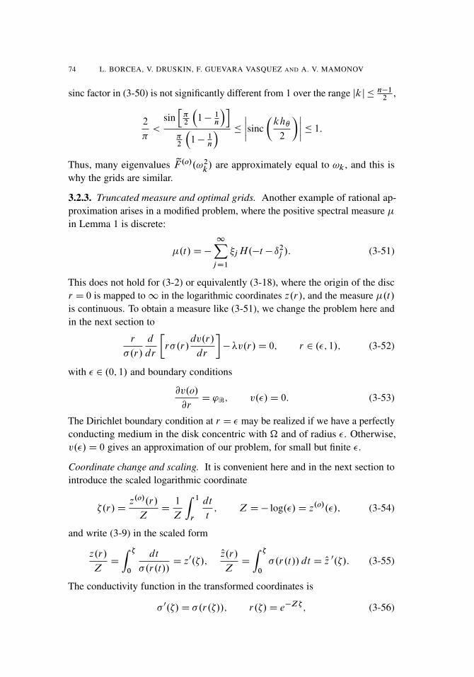
0 0.2 0.4 0.6 0.8 1
Figure 4. Example of a truncated measure optimal grid with` D 6. This is in the logarithmic scaled coordinates � 2 Œ0; 1�.The primary points are denoted with � and the dual ones with ı.
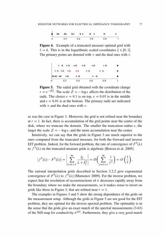
0 0.2 0.4 0.6 0.8 1
Figure 5. The radial grid obtained with the coordinate changer D e�Z� . The scale Z D� log � affects the distribution of theradii. The choice � D 0:1 is on top, � D 0:05 is in the middleand � D 0:01 is at the bottom. The primary radii are indicatedwith � and the dual ones with ı.
as was the case in Figure 3. Moreover, the grid is not refined near the boundaryat r D 1. In fact, there is accumulation of the grid points near the center of thedisk, where we truncate the domain. The smaller the truncation radius �, thelarger the scale Z D� log �, and the more accumulation near the center.
Intuitively, we can say that the grids in Figure 3 are much superior to theones computed from the truncated measure, for both the forward and inverseEIT problem. Indeed, for the forward problem, the rate of convergence of F|.�/
to f |.�/ on the truncated measure grids is algebraic [Borcea et al. 2005]
ˇf |.�/�F|.�/
ˇD
ˇˇ1X
jD`C1
�j
�C ı2j
ˇˇDO
� 1XjD`C1
1
j 2
�DO
�1
`
�:
The rational interpolation grids described in Section 3.2.2 give exponentialconvergence of F|.�/ to f |.�/ [Mamonov 2009]. For the inverse problem, weexpect that the resolution of reconstructions of � decreases rapidly away fromthe boundary where we make the measurements, so it makes sense to invert ongrids like those in Figure 3, that are refined near r D 1.
The examples in Figures 3 and 5 show the strong dependence of the grids onthe measurement setup. Although the grids in Figure 5 are not good for the EITproblem, they are optimal for the inverse spectral problem. The optimality is inthe sense that the grids give an exact match of the spectral measurements (3-63)of the NtD map for conductivity � .o/. Furthermore, they give a very good match

78 L. BORCEA, V. DRUSKIN, F. GUEVARA VASQUEZ AND A. V. MAMONOV
of the spectral measurements (3-68) for the unknown � , and the reconstructedconductivity on them converges to the true � , as we show next.
3.3. Continuum limit of the discrete inverse spectral problem on optimal grids.Let Qn W Dn! R2`
C be the reconstruction mapping that takes the data
Dn D˚�j ; ıj ; j D 1; : : : ; `
(3-68)
to the 2`Dn�1
2positive values f�j ; O�j gjD1;:::;` given by
�j DOj
O.o/j
; O�jC1 D˛.o/j
j; j D 1; 2; : : : ; `: (3-69)
The computation of f j ; Oj gjD1;:::;` requires solving the discrete inverse spectralproblem with data Dn, using for example the Lanczos algorithm reviewed inAppendix E. We define the reconstruction �`.�/ of the conductivity as thepiecewise constant interpolation of the point values (3-69) on the optimal grid(3-64). We have
�`.�/D
8<ˆ:�j if � 2 Œ�.o/j ; O�
.o/jC1
/; j D 1; : : : ; `;
O�j if � 2 Œ O�.o/j ; �.o/j /; j D 2; : : : ; `C 1;
O�`C1 if � 2 Œ�.o/lC1
; 1�;
(3-70)
and we discuss here its convergence to the true conductivity function �.�/, as`!1.
To state the convergence result, we need some assumptions on the decay withj of the perturbations of the spectral data
�ıj D ıj � ı.o/j ; ��j D �j � �
.o/j : (3-71)
The asymptotic behavior of ıj and �j is well known, under various smoothnessrequirements on �.z/ [McLaughlin and Rundell 1987; Pöschel and Trubowitz1987; Coleman and McLaughlin 1993]. For example, if �.�/ 2 H 3Œ0; 1�, wehave
�ıj D ıj � ı.o/j D
R 10 q.�/ d�
.2j � 1/�CO.j�2/ and ��j D �j � �
.o/j DO.j�2/;
(3-72)where q.�/ is the Schrödinger potential
q.�/D �.�/�12
d2�.�/12
d�2: (3-73)
We have the following convergence result proved in [Borcea et al. 2005].
RESISTOR NETWORKS FOR ELECTRICAL IMPEDANCE TOMOGRAPHY 79
Theorem 1. Suppose that �.�/ is a positive and bounded scalar conductivityfunction, with spectral data satisfying the asymptotic behavior
�ıj DO
�1
j s log.j /
�; ��j DO
�1
j s
�; for some s > 1; as j !1:
(3-74)Then �`.�/ converges to �.�/ as `!1, pointwise and in L1Œ0; 1�.
Before we outline the proof, let us note that it appears from (3-72) and (3-74)that the convergence result applies only to the class of conductivities with zeromean potential. However, if
q D
Z 1
0
q.�/ d� ¤ 0; (3-75)
we can modify the point values (3-69) of the reconstruction �`.�/ by replacing˛.o/j and O .o/j with ˛.q/j and O .q/j , for j D 1; : : : ; `. These are computed by
solving the discrete inverse spectral problem with data
D.q/n D f�.q/j ; ı
.q/j ; j D 1; : : : ; `g;
for the conductivity function
� .q/.�/D 14
�ep
q �C e�
pq ��2: (3-76)
This conductivity satisfies the initial value problem
d2p� .q/.�/
d�2D q
p� .q/.�/ for 0< � � 1;
d� .q/.0/
d�D 0 and � .q/.0/D 1;
(3-77)
and we assume that
q > ��2
4; (3-78)
so that (3-76) stays positive for � 2 Œ0; 1�.As seen from (3-72), the perturbations ıj � ı
.q/j and �j � �
.q/j satisfy the
assumptions (3-74), so Theorem 1 applies to reconstructions on the grid given by� .q/. We show below in Corollary 1 that this grid is asymptotically the same asthe optimal grid, calculated for � .o/. Thus, the convergence result in Theorem 1applies after all, without changing the definition of the reconstruction (3-70).

80 L. BORCEA, V. DRUSKIN, F. GUEVARA VASQUEZ AND A. V. MAMONOV
3.3.1. The case of constant Schrödinger potential. The equation (3-58) for � � .q/ can be transformed to Schrödinger form with constant potential q
d2w.�/
d�2� .�C q/w.�/D 0; � 2 .0; 1/;
dw.0/
d�D�1; w.1/D 0;
(3-79)
by letting w.�/D v.�/p� .q/.�/. Thus, the eigenfunctions y
.q/j .�/ of the differ-
ential operator associated with � .q/.�/ are related to y.o/j .�/, the eigenfunctions
for � .o/ � 1, by
y.q/j .�/D
y.o/j .�/p� .q/.�/
: (3-80)
They satisfy the orthonormality conditionZ 1
0
y.q/j .�/y.q/p .�/� .q/.�/ d� D
Z 1
0
y.o/j .�/y.o/p .�/ d� D ıjp; (3-81)
and since � .q/.0/D 1,
�.q/j D
�y.q/j .0/
�2D�y.o/j .0/
�2D �
.o/j ; j D 1; 2; : : : (3-82)
The eigenvalues are shifted by q:
��ı.q/j
�2D�
�ı.o/j
�2� q; j D 1; 2; : : : (3-83)
Let f˛.q/j ; O.q/j gjD1;:::;` be the parameters obtained by solving the discrete
inverse spectral problem with data D.q/n . The reconstruction mapping
Qn W D.q/n ! R2`
gives the sequence of 2`Dn�1
2pointwise values
�.q/j D
O.q/j
O.o/j
; O�.q/jC1D˛.o/j
˛.q/j
; j D 1; : : : ; `: (3-84)
We have the following result stated and proved in [Borcea et al. 2005]. See thereview of the proof in Appendix F.
Lemma 3. The point values � .q/j satisfy the finite difference discretization ofinitial value problem (3-77), on the optimal grid, namely

RESISTOR NETWORKS FOR ELECTRICAL IMPEDANCE TOMOGRAPHY 81
1
O.o/j
q�.q/jC1�
q�.q/j
˛.o/j
�
q�.q/j �
q�.q/j�1
˛.o/j � 1
�� q
q�.q/j D 0 (3-85)
for j D 2; 3; : : : ; `, and
1
O.o/1
q�.q/2�
q�.q/1
˛.o/1
� q
q�.q/1D 0; �
.q/1D 1: (3-86)
Moreover, O� .q/jC1D
q�.q/j �
.q/jC1
, for j D 1; : : : ; `.
The convergence of the reconstruction � .q/;`.�/ follows from this lemma anda standard finite-difference error analysis [Godunov and Ryabenki 1964] on theoptimal grid satisfying Lemma 2. The reconstruction is defined as in (3-70), bythe piecewise constant interpolation of the point values (3-84) on the optimalgrid.
Theorem 2. As `!1 we have
max1�j�`
ˇ�.q/j � � .q/.�
.o/j /
ˇ! 0 and max
1�j�`
ˇO�.q/jC1� � .q/. O�
.o/jC1
/ˇ! 0;
and the reconstruction � .q/;`.�/ converges to � .q/.�/ in L1Œ0; 1�.
As a corollary to this theorem, we can now obtain that the grid induced by� .q/.�/, with primary nodes �.q/j and dual nodes O�.q/j , is asymptotically close tothe optimal grid. The proof is in Appendix F.
Corollary 1. The grid induced by � .q/.�/ is defined by the equationsZ �.q/
jC1
0
d�
� .q/.�/D
jXpD1
˛.q/p ;
Z O�.q/jC1
0
� .q/.�/ d� D
jXpD1
O.q/p ; j D 1; : : : ; `;
�.q/1D O�
.q/1D 0; (3-87)
and satisfies
max1�j�`C1
ˇ�.q/j � �
.o/j
ˇ! 0; max
1�j�`C1
ˇO�.q/j � O�
.o/j
ˇ! 0; as `!1: (3-88)
3.3.2. Outline of the proof of Theorem 1. The proof given in detail in [Borceaet al. 2005] has two main steps. The first step is to establish the compactnessof the set of reconstructed conductivities. The second step uses the establishedcompactness and the uniqueness of solution of the continuum inverse spectralproblem to get the convergence result.
82 L. BORCEA, V. DRUSKIN, F. GUEVARA VASQUEZ AND A. V. MAMONOV
Step 1: Compactness. We show here that the sequence f�`.�/g`�1 of recon-structions (3-70) has bounded variation.
Lemma 4. The sequence f�j ; O�jC1gjD1;:::;` of (3-69) returned by the reconstruc-tion mapping Qn satisfies
XjD1
ˇlog O�jC1� log �j
ˇC
XjD1
ˇlog O�jC1� log �jC1
ˇ� C; (3-89)
where the constant C is independent of `. Therefore the sequence of reconstruc-tions f�`.�/g`�1 has uniformly bounded variation.
Our original formulation is not convenient for proving (3-89), because whenwritten in Schrödinger form, it involves the second derivative of the conductivity,as seen from (3-73). Thus, we rewrite the problem in first order system form,which involves only the first derivative of �.�/, which is all we need to show(3-89). At the discrete level, the linear system of ` equations
AV ��V D�e1
O1(3-90)
for the potential V D .V1; : : : ;V`/T is transformed into the system of 2` equations
BH12 W �
p�H
12 W D�
e1p� O1
(3-91)
for the vector W D .W1; yW2; : : : ;W`; yW`C1/T with components
Wj Dp�j Vj ; yWjC1 D
O�jC1p��j
VjC1�Vj
˛.o/j
; j D 1; : : : ; `: (3-92)
Here H D diag . O .o/1; ˛.o/1; : : : ; O
.o/
`; ˛.o/
`/ and B is the tridiagonal, skew-sym-
metric matrix
B D
0BBBBBB@
0 ˇ1 0 0 : : :
�ˇ1 0 ˇ2 0 : : :
0 �ˇ2 0: : :
::::::
0 : : : �ˇ2`�1 0
1CCCCCCA (3-93)
with entries
ˇ2p D1p
p OpC1
D1q
˛.o/p O
.o/p C 1
sO�pC1
�pD ˇ
.o/2p
sO�pC1
�pC1
(3-94)

RESISTOR NETWORKS FOR ELECTRICAL IMPEDANCE TOMOGRAPHY 83
and
ˇ2p�1 D1pp Op
D1q
˛.o/p O
.o/p
sO�pC1
�pD ˇ
.o/2p�1
sO�pC1
�p: (3-95)
Note that we have
2`�1XpD1
ˇˇlog p
ˇ.o/p
ˇˇ
D1
2
XpD1
ˇlog O�pC1� log �p
ˇC
1
2
XpD1
ˇlog O�pC1� log �pC1
ˇ; (3-96)
and we can prove (3-89) using the method of small perturbations. Recall defini-tions (3-71) and let
�ırj D r�ıj ; ��r
j D r��j ; j D 1; : : : ; `; (3-97)
where r 2 Œ0; 1� is an arbitrary continuation parameter. Let also ˇrj be the entries
of the tridiagonal, skew-symmetric matrix B r determined by the spectral dataırj D ı
.o/j C�ı
rj and �r
j D �.o/j C��
rj , for j D 1; : : : ; `. We explain in Appendix
G how to obtain explicit formulae for the perturbations d logˇrj in terms of the
eigenvalues and eigenvectors of matrix B r and perturbations dırj D�ıj dr and
d�rj D��j dr . These perturbations satisfy the uniform bound
2`�1XjD1
ˇd logˇr
j
ˇ� C1jdr j; (3-98)
with constant C1 independent of ` and r . Then,
log j
ˇ.o/j
D
Z 1
0
d logˇrj (3-99)
satisfies the uniform bound2`�1XjD1
ˇˇlog j
ˇ.o/j
ˇˇ� C1 and (3-89) follows from (3-96).
Step 2: Convergence. Recall from Section 3.2 that the eigenvectors Yj of A areorthonormal with respect to the weighted inner product (3-30). Then, the matrixzY with columns diag
�O
1=21; : : : ; O
1=2
`
�Yj is orthogonal and we have
. zY zY T /11 D O1
XjD1
�j D 1: (3-100)

84 L. BORCEA, V. DRUSKIN, F. GUEVARA VASQUEZ AND A. V. MAMONOV
Similarly
O.o/1
XjD1
�.o/j D 2` O
.o/1D 1; (3-101)
where we used (3-63), and since ��j are summable by assumption (3-74),
�1 DO1
O.o/1
D
�1C O
.o/1
XjD1
��j
��1
D 1CO. O.o/1/D 1CO
�1
`
�: (3-102)
But �`.0/D�1, and since �`.�/ has bounded variation by Lemma 4, we concludethat �`.�/ is uniformly bounded in � 2 Œ0; 1�.
Now, to show that �`.�/! �.�/ in L1Œ0; 1�, suppose for contradiction that itdoes not. Then, there exists " > 0 and a subsequence �`k such that
k�`k � �kL1Œ0;1� � ":
But since this subsequence is bounded and has bounded variation, we concludefrom Helly’s selection principle and the compactness of the embedding of thespace of functions of bounded variation in L1Œ0; 1� (see [Natanson 1955]) thatit has a subsequence that converges pointwise and in L1Œ0; 1�. Call again thissubsequence �`k and denote its limit by �? ¤ � . Since the limit is in L1Œ0; 1�,we have by definitions (3-55) and Remark 3,
z.�I �`k /D
Z �
0
dt
�`k .t/! z.�I �/D
Z �
0
dt
�?.t/;
Oz.�I �`k /D
Z �
0
�`k .t/ dt ! Oz.�I �?/D
Z �
0
�.t/ dt:
(3-103)
The continuity of f | with respect to the conductivity gives f |.�I �`k / !
f |.�I �?/. However, Lemma 1 and (3-51) show that f |.�I �`/! f |.�I �/
by construction, and since the inverse spectral problem has a unique solution[Gel’fand and Levitan 1951; Levitan 1987; Coleman and McLaughlin 1993;Pöschel and Trubowitz 1987], we must have �? D � . We have reached acontradiction, so �`.�/! �.�/ in L1Œ0; 1�. The pointwise convergence can beproved analogously.
Remark 4. All the elements of the proof presented here, except for establishingthe bound (3-98), apply to any measurement setup. The challenge in provingconvergence of inversion on optimal grids for general measurements lies entirelyin obtaining sharp stability estimates of the reconstructed sequence with respectto perturbations in the data. The inverse spectral problem is stable, and this iswhy we could establish the bound (3-98). The EIT problem is exponentially

RESISTOR NETWORKS FOR ELECTRICAL IMPEDANCE TOMOGRAPHY 85
unstable, and it remains an open problem to show the compactness of the functionspace of reconstruction sequences �` from measurements such as (3-49).
4. Two-dimensional media and full boundary measurements
We now consider the two-dimensional EIT problem, where � D �.r; �/ and wecannot use separation of variables as in Section 3. More explicitly, we cannotreduce the inverse problem for resistor networks to one of rational approximationof the eigenvalues of the DtN map. We start by reviewing in Section 4.1 theconditions of unique recovery of a network .�; / from its DtN mapƒ , definedby measurements of the continuum ƒ� . The approximation of the conductivity� from the network conductance function is described in Section 4.2.
4.1. The inverse problem for planar resistor networks. The unique recoverabil-ity fromƒ of a network .�; /with known circular planar graph � is establishedin [Colin de Verdière 1994; Colin de Verdière et al. 1996; Curtis et al. 1994;Curtis et al. 1998]. A graph � D .P;E/ is called circular and planar if it can beembedded in the plane with no edges crossing and with the boundary nodes lyingon a circle. We call by association the networks with such graphs circular planar.The recoverability result states that if the data is consistent and the graph � iscritical then the DtN map ƒ determines uniquely the conductance function .By consistent data we mean that the measured matrix ƒ belongs to the set ofDtN maps of circular planar resistor networks.
A graph is critical if and only if it is well-connected and the removal of anyedge breaks the well-connectedness. A graph is well-connected if all its circularpairs .P;Q/ are connected. Let P and Q be two sets of boundary nodes with thesame cardinality jP j D jQj. We say that .P;Q/ is a circular pair when the nodesin P and Q lie on disjoint segments of the boundary B. The pair is connected ifthere are jP j disjoint paths joining the nodes of P to the nodes of Q.
A symmetric n�n real matrix ƒ is the DtN map of a circular planar resistornetwork with n boundary nodes if its rows sum to zero ƒ 1D 0 (conservationof currents) and all its circular minors .ƒ /P;Q have nonpositive determinant.A circular minor .ƒ /P;Q is a square submatrix of ƒ defined for a circularpair .P;Q/, with row and column indices corresponding to the nodes in P andQ, ordered according to a predetermined orientation of the circle B. Sincesubsets of P and Q with the same cardinality also form circular pairs, thedeterminantal inequalities are equivalent to requiring that all circular minorsbe totally nonpositive. A matrix is totally nonpositive if all its minors havenonpositive determinant.
Examples of critical networks were given in Section 2.2, with graphs �determined by tensor product grids. Criticality of such networks is proved in
86 L. BORCEA, V. DRUSKIN, F. GUEVARA VASQUEZ AND A. V. MAMONOV
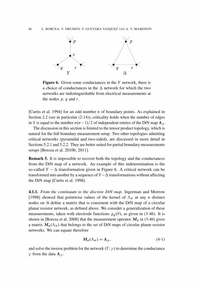
Yq r
s
p
q r�
p
Figure 6. Given some conductances in the Y network, there isa choice of conductances in the � network for which the twonetworks are indistinguishable from electrical measurements atthe nodes p, q and r .
[Curtis et al. 1994] for an odd number n of boundary points. As explained inSection 2.2 (see in particular (2-14)), criticality holds when the number of edgesin E is equal to the number n.n�1/=2 of independent entries of the DtN mapƒ .
The discussion in this section is limited to the tensor product topology, which isnatural for the full boundary measurement setup. Two other topologies admittingcritical networks (pyramidal and two-sided), are discussed in more detail inSections 5.2.1 and 5.2.2. They are better suited for partial boundary measurementssetups [Borcea et al. 2010b; 2011].
Remark 5. It is impossible to recover both the topology and the conductancesfrom the DtN map of a network. An example of this indetermination is theso-called Y �� transformation given in Figure 6. A critical network can betransformed into another by a sequence of Y�� transformations without affectingthe DtN map [Curtis et al. 1998].
4.1.1. From the continuum to the discrete DtN map. Ingerman and Morrow[1998] showed that pointwise values of the kernel of ƒ� at any n distinctnodes on B define a matrix that is consistent with the DtN map of a circularplanar resistor network, as defined above. We consider a generalization of thesemeasurements, taken with electrode functions �q.�/, as given in (3-46). It isshown in [Borcea et al. 2008] that the measurement operator Mn in (3-46) givesa matrix Mn.ƒ� / that belongs to the set of DtN maps of circular planar resistornetworks. We can equate therefore
Mn.ƒ� /Dƒ ; (4-1)
and solve the inverse problem for the network .�; / to determine the conductance from the data ƒ .

RESISTOR NETWORKS FOR ELECTRICAL IMPEDANCE TOMOGRAPHY 87
4.2. Solving the 2D problem with optimal grids. To approximate �.x/ fromthe network conductance we modify the reconstruction mapping introduced inSection 3.2 for layered media. The approximation is obtained by interpolatingthe output of the reconstruction mapping on the optimal grid computed for thereference � .o/ � 1. This grid is described in Sections 2.2 and 3.2.2. But whichinterpolation should we take? If we could have grids with as many points aswe wish, the choice of the interpolation would not matter. This was the casein Section 3.3, where we studied the continuum limit n!1 for the inversespectral problem. The EIT problem is exponentially unstable and the wholeidea of our approach is to have a sparse parametrization of the unknown � .Thus, n is typically small, and the approximation of � should go beyond ad-hocinterpolations of the parameters returned by the reconstruction mapping. Weshow in Section 4.2.3 how to approximate � with a Gauss–Newton iterationpreconditioned with the reconstruction mapping. We also explain briefly howone can introduce prior information about � in the inversion method.
4.2.1. The reconstruction mapping. The idea behind the reconstruction mappingis to interpret the resistor network .�; / determined from the measured ƒ DMn.ƒ� / as a finite-volume discretization of the equation (1-1) on the optimalgrid computed for � .o/ � 1. This is what we did in Section 3.2 for the layeredcase, and the approach extends to the two-dimensional problem.
The conductivity is related to the conductances .E/, for E2E, via quadraturerules that approximate the current fluxes (2-5) through the dual edges. We coulduse for example the quadrature in [Borcea et al. 2010a; 2010b; Mamonov 2010],where the conductances are
a;b D �.Pa;b/L.†a;b/
L.Ea;b/; .a; b/ 2
˚�i; j ˙ 1
2
�;�i ˙ 1
2; j�; (4-2)
where L denotes the arc length of the primary and dual edges E and † (seeSection 2.1 for the indexing and edge notation). Another example of quadratureis given in [Borcea et al. 2008]. It is specialized to tensor product grids in adisk, and it coincides with the quadrature (3-8) in the case of layered media. Forinversion purposes, the difference introduced by different quadrature rules issmall (see [Borcea et al. 2010a, Section 2.4]).
To define the reconstruction mapping Qn, we solve two inverse problems forresistor networks. One with the measured data ƒ DMn.ƒ� /, to determinethe conductance , and one with the computed data ƒ .o/ DMn.ƒ�.o//, for thereference � .o/ � 1. The latter gives the reference conductance .o/ which weassociate with the geometrical factor in (4-2)
.o/
a;b�
L.†a;b/
L.Ea;b/; (4-3)
88 L. BORCEA, V. DRUSKIN, F. GUEVARA VASQUEZ AND A. V. MAMONOV
so that we can write
�.Pa;b/� �a;b D a;b
.o/
a;b
: (4-4)
Note that (4-4) becomes (3-40) in the layered case, where (3-8) gives j D
h�= jC 12;q and Oj D h� j ;qC 1
2. The factors h� cancel out.
Let us call Dn the set in Re of e D n.n� 1/=2 independent measurementsin Mn.ƒ� /, obtained by removing the redundant entries. Note that there aree edges in the network, as many as the number of the data points in Dn, givenfor example by the entries in the upper triangular part of Mn.ƒ� /, stackedcolumn by column in a vector in Re. By the consistency of the measurements(Section 4.1.1), Dn coincides with the set of the strictly upper triangular parts ofthe DtN maps of circular planar resistor networks with n boundary nodes. Themapping Qn W Dn ! Re
C associates to the measurements in Dn the e positivevalues �a;b in (4-4).
We illustrate in Figure 7(b) the output of the mapping Qn, linearly interpolatedon the optimal grid. It gives a good approximation of the conductivity thatis improved further in Figure 7(c) with the Gauss–Newton iteration describedbelow. The results in Figure 7 are obtained by solving the inverse problem for thenetworks with a fast layer peeling algorithm [Curtis et al. 1994]. Optimizationcan also be used for this purpose, at some additional computational cost. In anycase, because we have relatively few n.n�1/=2 parameters, the cost is negligiblecompared to that of solving the forward problem on a fine grid.
4.2.2. The optimal grids and sensitivity functions. The definition of the tensorproduct optimal grids considered in Sections 2.2 and 3 does not extend to partialboundary measurement setups or to nonlayered reference conductivity functions.We present here an alternative approach to determining the location of thepoints Pa;b at which we approximate the conductivity in the output (4-4) ofthe reconstruction mapping. This approach extends to arbitrary setups, and it isbased on the sensitivity analysis of the conductance function to changes in theconductivity [Borcea et al. 2010b].
The sensitivity grid points are defined as the maxima of the sensitivity functionsD� a;b.x/. They are the points at which the conductances a;b are most sensitiveto changes in the conductivity. The sensitivity functions D� .x/ are obtainedby differentiating the identity ƒ .�/ DMn.ƒ� / with respect to � :
.D� / .x/D�D ƒ
ˇƒ DMn.ƒ� /
��1vec .Mn.DK� /.x// ; x 2�: (4-5)
The left-hand side is a vector in Re. Its k�th entry is the Fréchet derivative ofconductance k with respect to changes in the conductivity � . The entries of the
RESISTOR NETWORKS FOR ELECTRICAL IMPEDANCE TOMOGRAPHY 89
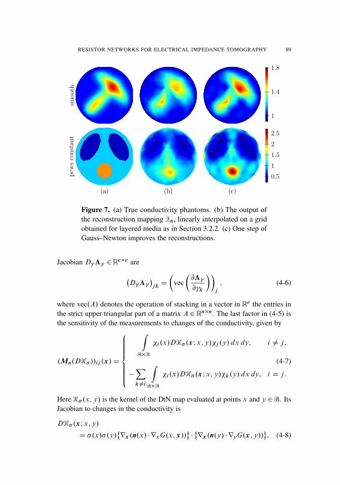
smooth
1
1.4
1.8pcw
sconstan
t
0.5
1
1.5
2
2.5
(a) (b) (c)
Figure 7. (a) True conductivity phantoms. (b) The output ofthe reconstruction mapping Qn, linearly interpolated on a gridobtained for layered media as in Section 3.2.2. (c) One step ofGauss–Newton improves the reconstructions.
Jacobian D ƒ 2 Re�e are
�D ƒ
�jkD
�vec
�@ƒ
@ k
��j
; (4-6)
where vec.A/ denotes the operation of stacking in a vector in Re the entries inthe strict upper triangular part of a matrix A 2 Rn�n. The last factor in (4-5) isthe sensitivity of the measurements to changes of the conductivity, given by
.Mn.DK� //ij .x/D
8ˆ<ˆ:
ZB�B
�i.x/DK� .xIx;y/�j .y/ dx dy, i ¤ j ,
�
Xk¤i
ZB�B
�i.x/DK� .xIx;y/�k.y/ dx dy, i D j .
(4-7)
Here K� .x;y/ is the kernel of the DtN map evaluated at points x and y 2B. ItsJacobian to changes in the conductivity is
DK� .xIx;y/
D �.x/�.y/˚rx.n.x/ � rxG.x;x//
�˚rx.n.y/ � ryG.x;y//
; (4-8)
90 L. BORCEA, V. DRUSKIN, F. GUEVARA VASQUEZ AND A. V. MAMONOV
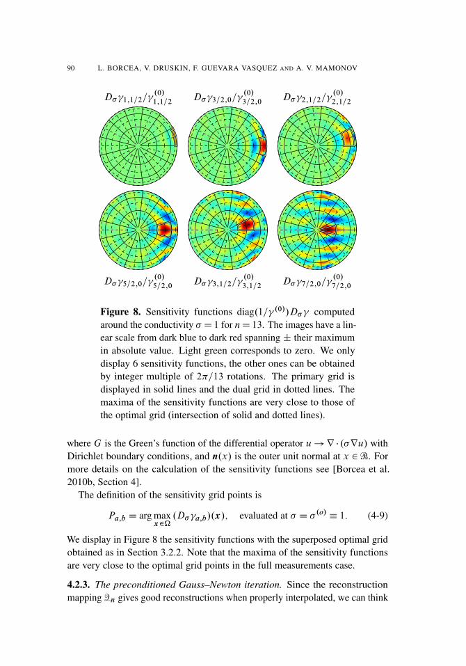
D� 1;1=2= .0/
1;1=2D� 3=2;0=
.0/
3=2;0D� 2;1=2=
.0/
2;1=2
D� 5=2;0= .0/
5=2;0D� 3;1=2=
.0/
3;1=2D� 7=2;0=
.0/
7=2;0
Figure 8. Sensitivity functions diag.1= .0//D� computedaround the conductivity � D 1 for nD 13. The images have a lin-ear scale from dark blue to dark red spanning ˙ their maximumin absolute value. Light green corresponds to zero. We onlydisplay 6 sensitivity functions, the other ones can be obtainedby integer multiple of 2�=13 rotations. The primary grid isdisplayed in solid lines and the dual grid in dotted lines. Themaxima of the sensitivity functions are very close to those ofthe optimal grid (intersection of solid and dotted lines).
where G is the Green’s function of the differential operator u!r � .�ru/ withDirichlet boundary conditions, and n.x/ is the outer unit normal at x 2B. Formore details on the calculation of the sensitivity functions see [Borcea et al.2010b, Section 4].
The definition of the sensitivity grid points is
Pa;b D arg maxx2�
.D� a;b/.x/; evaluated at � D � .o/ � 1: (4-9)
We display in Figure 8 the sensitivity functions with the superposed optimal gridobtained as in Section 3.2.2. Note that the maxima of the sensitivity functionsare very close to the optimal grid points in the full measurements case.
4.2.3. The preconditioned Gauss–Newton iteration. Since the reconstructionmapping Qn gives good reconstructions when properly interpolated, we can think
RESISTOR NETWORKS FOR ELECTRICAL IMPEDANCE TOMOGRAPHY 91
of it as an approximate inverse of the forward map Mn.ƒ� / and use it as anonlinear preconditioner. Instead of minimizing the misfit in the data, we solvethe optimization problem
min�>0
Qn.vec.Mn.ƒ� ///�Qn.vec.Mn.ƒ��/// 2
2: (4-10)
Here �� is the conductivity that we would like to recover. For simplicity theminimization (4-10) is formulated with noiseless data and no regularization. Werefer to [Borcea et al. 2011] for a study of the effect of noise and regularizationon the minimization (4-10).
The positivity constraints in (4-10) can be dealt with by solving for thelog-conductivity � D ln.�/ instead of the conductivity � . With this change ofvariable, the residual in (4-10) can be minimized with the standard Gauss–Newtoniteration, which we write in terms of the sensitivity functions (4-5) evaluated at� .j/ D exp �.j/:
�.jC1/D �.j/�
�diag.1= .0//D� diag.exp �.j//
�|��Qn.vec.Mn.ƒexp �.j ////�Qn.vec.Mn.ƒ��///
�: (4-11)
The superscript | denotes the Moore–Penrose pseudoinverse and the division isunderstood componentwise. We take as initial guess the log-conductivity �.0/ Dln � .0/, where � .0/ is given by the linear interpolation of Qn.vec.Mn.ƒ��// onthe optimal grid (i.e., the reconstruction from Section 4.2.1). Having such agood initial guess helps with the convergence of the Gauss–Newton iteration.Our numerical experiments indicate that the residual in (4-10) is mostly reducedin the first iteration [Borcea et al. 2008]. Subsequent iterations do not changesignificantly the reconstructions and result in negligible reductions of the residualin (4-10). Thus, for all practical purposes, the preconditioned problem is linear.We have also observed in [Borcea et al. 2008; 2011] that the conditioning of thelinearized problem is significantly reduced by the preconditioner Qn.
Remark 6. The conductivity obtained after one step of the Gauss–Newtoniteration is in the span of the sensitivity functions (4-5). The use of the sensitivityfunctions as an optimal parametrization of the unknown conductivity was studiedin [Borcea et al. 2011]. Moreover, the same preconditioned Gauss–Newtonidea was used in [Guevara Vasquez 2006] for the inverse spectral problem ofSection 3.2.
We illustrate the improvement of the reconstructions with one Gauss–Newtonstep in Figure 7 (c). If prior information about the conductivity is available, itcan be added in the form of a regularization term in (4-10). An example usingtotal variation regularization is given in [Borcea et al. 2008].

92 L. BORCEA, V. DRUSKIN, F. GUEVARA VASQUEZ AND A. V. MAMONOV
5. Two-dimensional media and partial boundary measurements
In this section we consider the two-dimensional EIT problem with partial bound-ary measurements. As mentioned in Section 1, the boundary B is the union of theaccessible subset BA and the inaccessible subset BI . The accessible boundaryBA may consist of one or multiple connected components. We assume that theinaccessible boundary is grounded, so the partial boundary measurements are aset of Cauchy data
˚ujBA
; .�n � ru/jBA
, where u satisfies (1-1) and ujBI
D 0.The inverse problem is to determine � from these Cauchy data.
Our inversion method described in the previous sections extends to the partialboundary measurement setup. But there is a significant difference concerningthe definition of the optimal grids. The tensor product grids considered so farare essentially one-dimensional, and they rely on the rotational invariance of theproblem for � .o/ � 1. This invariance does not hold for the partial boundarymeasurements, so new ideas are needed to define the optimal grids. We presenttwo approaches in Sections 5.1 and 5.2. The first one uses circular planarnetworks with the same topology as before, and mappings that take uniformlydistributed points on B to points on the accessible boundary BA. The secondone uses networks with topologies designed specifically for the partial boundarymeasurement setups. The underlying two-dimensional optimal grids are definedwith sensitivity functions.
5.1. Coordinate transformations for the partial data problem. The idea of theapproach described in this section is to map the partial data problem to onewith full measurements at equidistant points, where we know from Section 4how to define the optimal grids. Since � is a unit disk, we can do this withdiffeomorphisms of the unit disk to itself.
Let us denote such a diffeomorphism by F and its inverse F�1 by G. If thepotential u satisfies (1-1), then the transformed potential Qu.x/D u.F.x// solvesthe same equation with conductivity z� defined by
z�.x/DG0.y/�.y/ .G0.y//
T
jdet G0.y/j
ˇˇyDF.x/
; (5-1)
where G0 denotes the Jacobian of G. The conductivity z� is the push forwardof � by G, and it is denoted by G�� . Note that if G0.y/ .G0.y//
T¤ I and
det G0.y/¤ 0, then z� is a symmetric positive definite tensor. If its eigenvaluesare distinct, then the push forward of an isotropic conductivity is anisotropic.
The push forward g�ƒ� of the DtN map is written in terms of the restrictionsof diffeomorphisms G and F to the boundary. We call these restrictions gD GjB
RESISTOR NETWORKS FOR ELECTRICAL IMPEDANCE TOMOGRAPHY 93
and f D F jB and write
..g�ƒ� /uB/.�/D .ƒ� .uB ıg//.�/j�Df .�/ ; � 2 Œ0; 2�/; (5-2)
for uB 2H 1=2.B/. It is shown in [Sylvester 1990] that the DtN map is invariantunder the push forward in the following sense
g�ƒ� DƒG�� : (5-3)
Therefore, given (5-3) we can compute the push forward of the DtN map, solvethe inverse problem with data g�ƒ� to obtain G�� , and then map it back usingthe inverse of (5-2). This requires the full knowledge of the DtN map. However,if we use the discrete analogue of the above procedure, we can transform thediscrete measurements of ƒ� on BA to discrete measurements at equidistantpoints on B, from which we can estimate z� as described in Section 4.
There is a major obstacle to this procedure: The EIT problem is uniquelysolvable only for isotropic conductivities. Anisotropic conductivities are de-termined by the DtN map only up to a boundary-preserving diffeomorphism[Sylvester 1990]. Two distinct approaches to overcome this obstacle are describedin Sections 5.1.1 and 5.1.2. The first uses conformal mappings F and G thatpreserve the isotropy of the conductivity at the expense of rigid placement ofthe measurement points. The second approach uses extremal quasiconformalmappings that minimize the artificial anisotropy of z� introduced by the placementat our will of the measurement points in BA.
5.1.1. Conformal mappings. The push forward G�� of an isotropic � is isotropicif G and F satisfy G0
�.G0/T
�D I and F 0
�.F 0/T
�D I . This means that the
diffeomorphism is conformal and the push forward is simply
G�� D � ıF: (5-4)
Since all conformal mappings of the unit disk to itself belong to the family ofMöbius transforms [Lavrentiev and Shabat 1987], F must be of the form
F.z/D ei! z� a
1� az; z 2 C; jzj � 1; ! 2 Œ0; 2�/; a 2 C; jaj< 1; (5-5)
where we associate R2 with the complex plane C. Note that the group oftransformations (5-5) is extremely rigid, its only degrees of freedom being thenumerical parameters a and !.
To use the full data discrete inversion procedure from Section 4 we requirethat G maps the accessible boundary segment BA D
˚ei� j � 2 Œ�ˇ; ˇ�
to the
whole boundary with the exception of one segment between the equidistantmeasurement points �k , k D .nC 1/=2; .nC 3/=2 as shown in Figure 9. Thisdetermines completely the values of the parameters a and ! in (5-5) which in

94 L. BORCEA, V. DRUSKIN, F. GUEVARA VASQUEZ AND A. V. MAMONOV
α = θn+12
−α = θn+32
β = τ n+12
−β = τ n+32
Figure 9. The optimal grid in the unit disk (left) and its imageunder the conformal mapping F (right). Primary grid lines aresolid black, dual grid lines are dotted black. Boundary gridnodes: primary �, dual ı. The accessible boundary segment BA
is indicated by the outermost arc (thick solid line).
turn determine the mapping f on the boundary. Thus, we have no further controlover the positioning of the measurement points �k D f .�k/, k D 1; : : : ; n.
As shown in Figure 9 the lack of control over �k leads to a grid that is highlynonuniform in angle. In fact it is demonstrated in [Borcea et al. 2010a] thatas n increases there is no asymptotic refinement of the grid away from thecenter of BA, where the points accumulate. However, since the limit n!1 isunattainable in practice due to the severe ill-conditioning of the problem, thegrids obtained by conformal mapping can still be useful in practical inversion.We show reconstructions with these grids in Section 5.3.
5.1.2. Extremal quasiconformal mappings. To overcome the issues with confor-mal mappings that arise due to the inherent rigidity of the group of conformalautomorphisms of the unit disk, we use here quasiconformal mappings. Aquasiconformal mapping F obeys a Beltrami equation in �
@F
@zD �.z/
@F
@z; k�k1 < 1; (5-6)
with a Beltrami coefficient �.z/ that measures how much F differs from aconformal mapping. If � � 0, then (5-6) reduces to the Cauchy–Riemannequation and F is conformal. The magnitude of � also provides a measure ofthe anisotropy � of the push forward of � by F . The anisotropy is defined by
�.F��; z/D
p�1.z/=�2.z/� 1p�1.z/=�2.z/C 1
; (5-7)
RESISTOR NETWORKS FOR ELECTRICAL IMPEDANCE TOMOGRAPHY 95
where �1.z/ and �2.z/ are the largest and smallest eigenvalues of F�� respec-tively. The connection between � and � is given by
� .F��; z/D j�.z/j; (5-8)
and the maximum anisotropy is
�.F��/D supz�.F��; z/D k�k1: (5-9)
Since the unknown conductivity is isotropic, we would like to minimize theamount of artificial anisotropy that we introduce into the reconstruction by usingF . This can be done with extremal quasiconformal mappings, which minimizek�k1 under constraints that fix f D F jB, thus allowing us to control thepositioning of the measurement points �k D f .�k/, for k D 1; : : : ; n.
For sufficiently regular boundary values f there exists a unique extremalquasiconformal mapping that is known to be of a Teichmüller type [Strebel1976]. Its Beltrami coefficient satisfies
�.z/D k�k1�.z/
j�.z/j; (5-10)
for some holomorphic function �.z/ in �. Similarly, we can define the Beltramicoefficient for G, using a holomorphic function . It is established in [Reich1976] that F admits a decomposition
F D‰�1ıAK ıˆ; (5-11)
whereˆ.z/D
Z p�.z/dz; ‰.�/D
Z p .�/d�; (5-12)
are conformal away from the zeros of � and , and
AK .xC iy/DKxC iy (5-13)
is an affine stretch, the only source of anisotropy in (5-11):
� .F��/D k�k1 D
ˇK� 1
KC 1
ˇ: (5-14)
Since only the behavior of f at the measurement points �k is of interest to us,it is possible to construct explicitly the mappings ˆ and ‰ [Borcea et al. 2010a].They are Schwartz–Christoffel conformal mappings of the unit disk to polygonsof special form, as shown in Figure 10. See [Borcea et al. 2010a, Section 3.4]for more details.
We demonstrate the behavior of the optimal grids under the extremal quasi-conformal mappings in Figure 11. We present the results for two different values
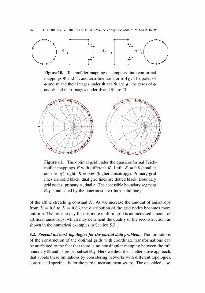
96 L. BORCEA, V. DRUSKIN, F. GUEVARA VASQUEZ AND A. V. MAMONOV
Φ AK Ψ−1
Figure 10. Teichmüller mapping decomposed into conformalmappings ˆ and ‰, and an affine transform AK . The poles of� and and their images under ˆ and ‰ areF, the zeros of �and and their images under ˆ and ‰ are �.
Figure 11. The optimal grid under the quasiconformal Teich-müller mappings F with different K. Left: K D 0:8 (smalleranisotropy); right: K D 0:66 (higher anisotropy). Primary gridlines are solid black, dual grid lines are dotted black. Boundarygrid nodes: primary �, dual ı. The accessible boundary segmentBA is indicated by the outermost arc (thick solid line).
of the affine stretching constant K. As we increase the amount of anisotropyfrom K D 0:8 to K D 0:66, the distribution of the grid nodes becomes moreuniform. The price to pay for this more uniform grid is an increased amount ofartificial anisotropy, which may detriment the quality of the reconstruction, asshown in the numerical examples in Section 5.3.
5.2. Special network topologies for the partial data problem. The limitationsof the construction of the optimal grids with coordinate transformations canbe attributed to the fact that there is no nonsingular mapping between the fullboundary B and its proper subset BA. Here we describe an alternative approach,that avoids these limitations by considering networks with different topologies,constructed specifically for the partial measurement setups. The one-sided case,
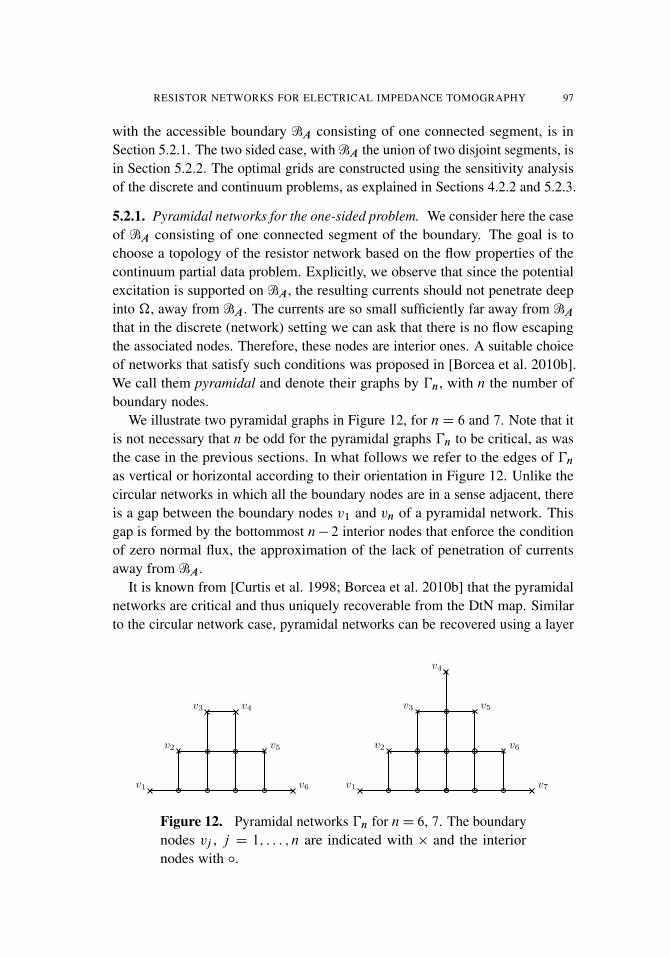
RESISTOR NETWORKS FOR ELECTRICAL IMPEDANCE TOMOGRAPHY 97
with the accessible boundary BA consisting of one connected segment, is inSection 5.2.1. The two sided case, with BA the union of two disjoint segments, isin Section 5.2.2. The optimal grids are constructed using the sensitivity analysisof the discrete and continuum problems, as explained in Sections 4.2.2 and 5.2.3.
5.2.1. Pyramidal networks for the one-sided problem. We consider here the caseof BA consisting of one connected segment of the boundary. The goal is tochoose a topology of the resistor network based on the flow properties of thecontinuum partial data problem. Explicitly, we observe that since the potentialexcitation is supported on BA, the resulting currents should not penetrate deepinto �, away from BA. The currents are so small sufficiently far away from BA
that in the discrete (network) setting we can ask that there is no flow escapingthe associated nodes. Therefore, these nodes are interior ones. A suitable choiceof networks that satisfy such conditions was proposed in [Borcea et al. 2010b].We call them pyramidal and denote their graphs by �n, with n the number ofboundary nodes.
We illustrate two pyramidal graphs in Figure 12, for nD 6 and 7. Note that itis not necessary that n be odd for the pyramidal graphs �n to be critical, as wasthe case in the previous sections. In what follows we refer to the edges of �n
as vertical or horizontal according to their orientation in Figure 12. Unlike thecircular networks in which all the boundary nodes are in a sense adjacent, thereis a gap between the boundary nodes v1 and vn of a pyramidal network. Thisgap is formed by the bottommost n� 2 interior nodes that enforce the conditionof zero normal flux, the approximation of the lack of penetration of currentsaway from BA.
It is known from [Curtis et al. 1998; Borcea et al. 2010b] that the pyramidalnetworks are critical and thus uniquely recoverable from the DtN map. Similarto the circular network case, pyramidal networks can be recovered using a layer
v1
v2
v3 v4
v5
v6 v1
v2
v3
v4
v5
v6
v7
Figure 12. Pyramidal networks �n for nD 6, 7. The boundarynodes vj , j D 1; : : : ; n are indicated with � and the interiornodes with ı.
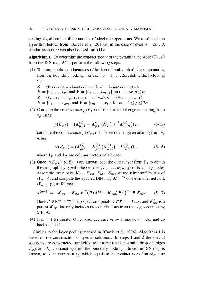
98 L. BORCEA, V. DRUSKIN, F. GUEVARA VASQUEZ AND A. V. MAMONOV
peeling algorithm in a finite number of algebraic operations. We recall such analgorithm below, from [Borcea et al. 2010b], in the case of even n D 2m. Asimilar procedure can also be used for odd n.
Algorithm 1. To determine the conductance of the pyramidal network .�n; /
from the DtN map ƒ.n/, perform the following steps:
(1) To compute the conductances of horizontal and vertical edges emanatingfrom the boundary node vp, for each p D 1; : : : ; 2m, define the followingsets:Z D fv1; : : : ; vp�1; vpC1; : : : ; vmg, C D fvmC2; : : : ; v2mg,H D fv1; : : : ; vpg and V D fvp; : : : ; vmC1g, in the case p �m.Z D fvmC1; : : : ; vp�1; vpC1; : : : ; v2mg, C D fv1; : : : ; vm�1g,H D fvp; : : : ; v2mg and V D fvm; : : : ; vpg, for mC 1� p � 2m.
(2) Compute the conductance .Ep;h/ of the horizontal edge emanating fromvp using
.Ep;h/D�ƒ.n/p;H� ƒ
.n/p;C
�ƒ.n/Z;C
��1ƒ.n/Z;H
�1H I (5-15)
compute the conductance .Ep;v/ of the vertical edge emanating from vpusing
.Ep;v/D�ƒ.n/p;V� ƒ
.n/p;C
�ƒ.n/Z;C
��1ƒ.n/Z;V
�1V ; (5-16)
where 1V and 1H are column vectors of all ones.
(3) Once .Ep;h/, .Ep;v/ are known, peel the outer layer from �n to obtainthe subgraph �n�2 with the set SD fw1; : : : ; w2m�2g of boundary nodes.Assemble the blocks KSS, KSB, KBS, KBB of the Kirchhoff matrix of.�n; /, and compute the updated DtN map ƒ.n�2/ of the smaller network.�n�2; /, as follows
ƒ.n�2/D�K 0SS � KSB P T
�P .ƒ.n/�KBB/P
T��1
P KBS: (5-17)
Here P 2 R.n�2/�n is a projection operator: PP T D In�2, and K 0SS is apart of KSS that only includes the contributions from the edges connectingS to B.
(4) If mD 1 terminate. Otherwise, decrease m by 1, update nD 2m and goback to step 1.
Similar to the layer peeling method in [Curtis et al. 1994], Algorithm 1 isbased on the construction of special solutions. In steps 1 and 2 the specialsolutions are constructed implicitly, to enforce a unit potential drop on edgesEp;h and Ep;v emanating from the boundary node vp. Since the DtN map isknown, so is the current at vp, which equals to the conductance of an edge due
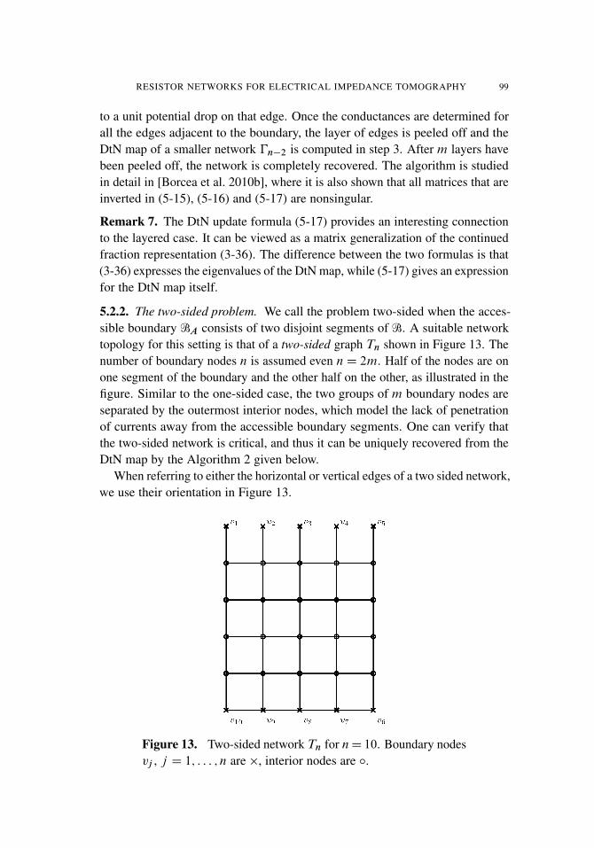
RESISTOR NETWORKS FOR ELECTRICAL IMPEDANCE TOMOGRAPHY 99
to a unit potential drop on that edge. Once the conductances are determined forall the edges adjacent to the boundary, the layer of edges is peeled off and theDtN map of a smaller network �n�2 is computed in step 3. After m layers havebeen peeled off, the network is completely recovered. The algorithm is studiedin detail in [Borcea et al. 2010b], where it is also shown that all matrices that areinverted in (5-15), (5-16) and (5-17) are nonsingular.
Remark 7. The DtN update formula (5-17) provides an interesting connectionto the layered case. It can be viewed as a matrix generalization of the continuedfraction representation (3-36). The difference between the two formulas is that(3-36) expresses the eigenvalues of the DtN map, while (5-17) gives an expressionfor the DtN map itself.
5.2.2. The two-sided problem. We call the problem two-sided when the acces-sible boundary BA consists of two disjoint segments of B. A suitable networktopology for this setting is that of a two-sided graph Tn shown in Figure 13. Thenumber of boundary nodes n is assumed even nD 2m. Half of the nodes are onone segment of the boundary and the other half on the other, as illustrated in thefigure. Similar to the one-sided case, the two groups of m boundary nodes areseparated by the outermost interior nodes, which model the lack of penetrationof currents away from the accessible boundary segments. One can verify thatthe two-sided network is critical, and thus it can be uniquely recovered from theDtN map by the Algorithm 2 given below.
When referring to either the horizontal or vertical edges of a two sided network,we use their orientation in Figure 13.
Figure 13. Two-sided network Tn for nD 10. Boundary nodesvj , j D 1; : : : ; n are �, interior nodes are ı.
100 L. BORCEA, V. DRUSKIN, F. GUEVARA VASQUEZ AND A. V. MAMONOV
Algorithm 2. To determine the conductance of the two-sided network .Tn; /
from the DtN map ƒ , perform the following steps:
(1) Peel the lower layer of horizontal resistors:For p DmC 2;mC 3; : : : ; 2m define the sets
Z D fpC 1;pC 2; : : : ;pCm� 1g and C D fp� 2;p� 3; : : : ;p�mg:
The conductance of the edge Ep;q;h between vp and vq , where q D p� 1,is given by
.Ep;q;h/D�ƒp;qCƒp;C .ƒZ;C /�1ƒZ;q: (5-18)
Assemble a symmetric tridiagonal matrix A with off-diagonal entries
� .Ep;p�1;h/
and rows summing to zero. Update the lower right m-by-m block of theDtN map by subtracting A from it.
(2) Let s Dm� 1.
(3) Peel the top and bottom layers of vertical resistors:For p D 1; 2; : : : ; 2m define the sets L D fp � 1;p � 2; : : : ;p � sg andRD fpC1;pC2; : : : ;pC sg. If p <m=2 for the top layer, or p > 3m=2
for the bottom layer, set Z D L, C D R. Otherwise let Z D R, C D L.The conductance of the vertical edge emanating from vp is given by
.Ep;v/Dƒp;p �ƒp;C .ƒZ;C /�1ƒZ;p: (5-19)
Let D D diag� .Ep;v/
�and update the DtN map
ƒ D�D �D�ƒ CD
��1D: (5-20)
(4) If s D 1 go to step (7). Otherwise decrease s by 2.
(5) Peel the top and bottom layers of horizontal resistors:For p D 1; 2; : : : ; 2m define the sets L D fp � 1;p � 2; : : : ;p � sg andR D fp C 2;p C 3; : : : ;p C s C 1g. If p < m=2 for the top layer, orp < 3m=2 for the bottom layer, set Z DL, C DR, q D pC 1. Otherwiselet Z DR, C DL, q D p� 1. The conductance of the edge connecting vpand vq is given by (5-18). Update the upper left and lower right blocks ofthe DtN map as in step (1).
(6) If s D 0 go to step (7), otherwise go to (3).
(7) Determine the last layer of resistors. If m is odd the remaining verticalresistors are the diagonal entries of the DtN map. If m is even, the remainingresistors are horizontal. The leftmost of the remaining horizontal resistors

RESISTOR NETWORKS FOR ELECTRICAL IMPEDANCE TOMOGRAPHY 101
.E1;2;h/ is determined from (5-18) with p D 1, q DmC 1, C D f1; 2g,Z D fmC 1;mC 2g and a change of sign. The rest are determined by
.Ep;pC1;h/D�ƒp;H � ƒp;C .ƒZ;C /
�1ƒZ;H
�1; (5-21)
where p D 2; 3; : : : ;m� 1,
C D fp� 1;p;pC 1g; Z D fpCm� 1;pCm;pCmC 1g;
H D fpCm� 1;pCmg; 1D .1; 1/T :
Similar to Algorithm 1, Algorithm 2 is based on the construction of specialsolutions examined in [Curtis et al. 1994; Curtis and Morrow 2000]. Thesesolutions are designed to localize the flow on the outermost edges, whose conduc-tance we determine first. In particular, formulas (5-18) and (5-19) are known asthe “boundary edge” and “boundary spike” formulas [Curtis and Morrow 2000,Corollaries 3.15 and 3.16].
5.2.3. Sensitivity grids for pyramidal and two-sided networks. The underlyinggrids of the pyramidal and two-sided networks are truly two-dimensional, andthey cannot be constructed explicitly as in Section 3 by reducing the problem to aone-dimensional one. We define the grids with the sensitivity function approachdescribed in Section 4.2.2. The computed sensitivity grid points are presentedin Figure 14, and we observe a few important properties. First, the neighboringpoints corresponding to the same type of resistors (vertical or horizontal) form
Figure 14. Sensitivity optimal grids in the unit disk for thepyramidal network �n (left) and the two-sided network Tn (right)with nD16. The accessible boundary segments BA are solid red.The symbol � corresponds to vertical edges,F corresponds tohorizontal edges, and measurement points are marked with �.

102 L. BORCEA, V. DRUSKIN, F. GUEVARA VASQUEZ AND A. V. MAMONOV
rather regular virtual quadrilaterals. Second, the points corresponding to differenttypes of resistors interlace in the sense of lying inside the virtual quadrilateralsformed by the neighboring points of the other type. Finally, while there is somerefinement near the accessible boundary (more pronounced in the two-sided case),the grids remain quite uniform throughout the covered portion of the domain.
Note from Figure 13 that the graph Tn lacks upside-down symmetry. Thus,it is possible to come up with two sets of optimal grid nodes, by fitting themeasured DtN map Mn.ƒ� / once with a two-sided network and the secondtime with the network turned upside-down. This way the number of nodes in thegrid is essentially doubled, thus doubling the resolution of the reconstruction.However, this approach can only improve resolution in the direction transversalto the depth.
5.3. Numerical results. We present in this section numerical reconstructionswith partial boundary measurements. The reconstructions with the four methodsfrom Sections 5.1.1, 5.1.2, 5.2.1 and 5.2.2 are compared row by row in Figure 15.We use the same two test conductivities as in Figure 7(a). Each row in Figure 15corresponds to one method. For each test conductivity, we show first the piecewiselinear interpolation of the entries returned by the reconstruction mapping Qn, onthe optimal grids (first and third column in Figure 15). Since these grids do notcover the entire�, we display the results only in the subset of� populated by thegrid points. We also show the reconstructions after one-step of the Gauss–Newtoniteration (4-11) (second and fourth columns in Figure 15).
As expected, reconstructions with the conformal mapping grids are the worst.The highly nonuniform conformal mapping grids cannot capture the details ofthe conductivities away from the middle of the accessible boundary. The recon-structions with quasiconformal grids perform much better, capturing the detailsof the conductivities much more uniformly throughout the domain. Although thepiecewise linear reconstructions Qn have slight distortions in the geometry, thesedistortions are later removed by the first step of the Gauss–Newton iteration.The piecewise linear reconstructions with pyramidal and two-sided networksavoid the geometrical distortions of the quasiconformal case, but they are alsoimproved after one step of the Gauss–Newton iteration.
Note that while the Gauss–Newton step improves the geometry of the recon-structions, it also introduces some spurious oscillations. This is more pronouncedfor the piecewise constant conductivity phantom (fourth column in Figure 15). Toovercome this problem one may consider regularizing the Gauss–Newton iteration(4-11) by adding a penalty term of some sort. For example, for the piecewiseconstant phantom, we could penalize the total variation of the reconstruction, aswas done in [Borcea et al. 2008].

RESISTOR NETWORKS FOR ELECTRICAL IMPEDANCE TOMOGRAPHY 103
Figure 15. Reconstructions with partial data. Same conduc-tivities are used as in Figure 7. Two leftmost columns: smoothconductivity. Two rightmost columns: piecewise constant chestphantom. Columns 1 and 3: piecewise linear reconstructions.Columns 2 and 4: reconstructions after one step of Gauss–Newton iteration (4-11). Rows from top to bottom: conformalmapping, quasiconformal mapping, pyramidal network, two-sided network. The accessible boundary BA is indicated bysolid arcs exterior to each disk. The centers of supports ofmeasurement (electrode) functions �q are marked with �.
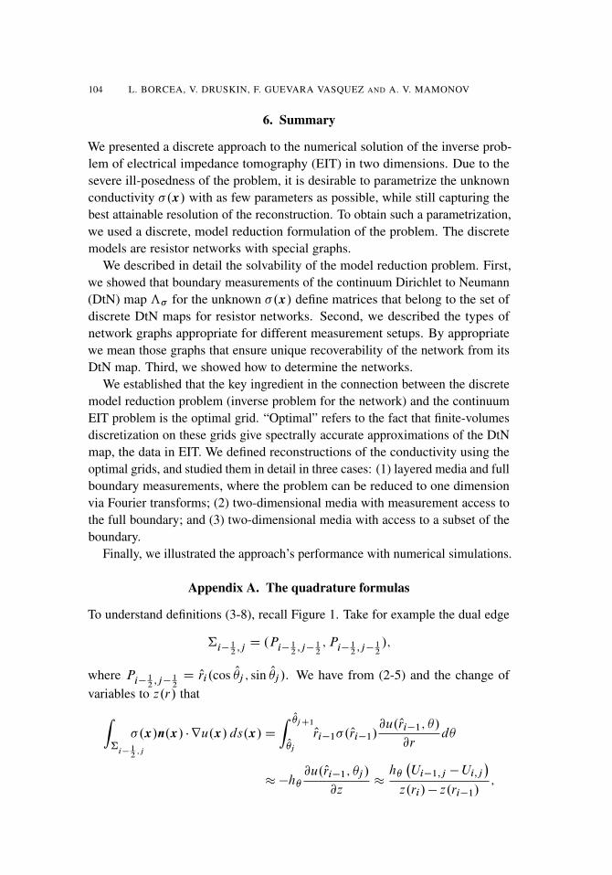
104 L. BORCEA, V. DRUSKIN, F. GUEVARA VASQUEZ AND A. V. MAMONOV
6. Summary
We presented a discrete approach to the numerical solution of the inverse prob-lem of electrical impedance tomography (EIT) in two dimensions. Due to thesevere ill-posedness of the problem, it is desirable to parametrize the unknownconductivity �.x/ with as few parameters as possible, while still capturing thebest attainable resolution of the reconstruction. To obtain such a parametrization,we used a discrete, model reduction formulation of the problem. The discretemodels are resistor networks with special graphs.
We described in detail the solvability of the model reduction problem. First,we showed that boundary measurements of the continuum Dirichlet to Neumann(DtN) map ƒ� for the unknown �.x/ define matrices that belong to the set ofdiscrete DtN maps for resistor networks. Second, we described the types ofnetwork graphs appropriate for different measurement setups. By appropriatewe mean those graphs that ensure unique recoverability of the network from itsDtN map. Third, we showed how to determine the networks.
We established that the key ingredient in the connection between the discretemodel reduction problem (inverse problem for the network) and the continuumEIT problem is the optimal grid. “Optimal” refers to the fact that finite-volumesdiscretization on these grids give spectrally accurate approximations of the DtNmap, the data in EIT. We defined reconstructions of the conductivity using theoptimal grids, and studied them in detail in three cases: (1) layered media and fullboundary measurements, where the problem can be reduced to one dimensionvia Fourier transforms; (2) two-dimensional media with measurement access tothe full boundary; and (3) two-dimensional media with access to a subset of theboundary.
Finally, we illustrated the approach’s performance with numerical simulations.
Appendix A. The quadrature formulas
To understand definitions (3-8), recall Figure 1. Take for example the dual edge
†i� 12;j D .Pi� 1
2;j� 1
2;Pi� 1
2;j� 1
2/;
where Pi� 12;j� 1
2D Ori.cos O�j ; sin O�j /. We have from (2-5) and the change of
variables to z.r/ thatZ†
i� 12;j
�.x/n.x/ � ru.x/ ds.x/D
Z O�jC1
O�j
Ori�1�. Ori�1/@u. Ori�1; �/
@rd�
��h�@u. Ori�1; �j /
@z�
h��Ui�1;j �Ui;j
�z.ri/� z.ri�1/
;
RESISTOR NETWORKS FOR ELECTRICAL IMPEDANCE TOMOGRAPHY 105
which gives the first equation in (3-8). Similarly, the flux across
†i;jC 12D .Pi� 1
2;jC 1
2;PiC 1
2;jC 1
2/
is given byZ†
i;jC 12
�.x/n.x/ � ru.x/ ds.x/D
Z Ori�1
Ori
�.r/
r
@u.r; O�jC1/
@�dr
�@u.ri ; O�jC1/
@�
Z Ori�1
Ori
�.r/
rdr
� .Oz. Ori/� Oz. Ori�1//Ui;jC1�U.i; j /
h�;
which gives the second equation in (3-8).
Appendix B. Continued fraction representation
Let us begin with the system of equations satisfied by the potential Vj , whichwe rewrite as
bj D bjC1C OjC1�VjC1 .0; 1; : : : ; `/; b0 DˆB; V`C1 D 0; (B-1)
where we letVj D VjC1C j bj : (B-2)
Combining the first equation in (B-1) with (B-2), we obtain the recursive relation
bj
VjD
1
jC1
OjC1�CbjC1
VjC1
; j D 1; 2; : : : ; `; (B-3)
which we iterate for j decreasing from j D `� 1 to 1, and starting with
b`
V`D
1
˛`: (B-4)
The latter follows from the first equation in (B-1) evaluated at j D`, and boundarycondition V`C1 D 0. We obtain that
F|.�/D V1=ˆB DV1
b0
DV1
b1C O1�V1D
1
O1�Cb1
V1
(B-5)
has the continued fraction representation (3-36).
106 L. BORCEA, V. DRUSKIN, F. GUEVARA VASQUEZ AND A. V. MAMONOV
Appendix C. Derivation of (3-47) and (3-48)
To derive (3-47) let us begin with the Fourier series of the electrode functions
�q.�/DXk2Z
Cq.k/eik�D
Xk2Z
Cq.k/e�ik� ; (C-1)
where the bar denotes complex conjugate and the coefficients are
Cq.�/D1
2�
Z 2�
0
�q.�/eik�d� D
eik�q
2�sinc
�kh�
2
�: (C-2)
Then, we have
.ƒ /p;q D
Z 2�
0
�p.�/ƒ��q.�/ d� DX
k;k02Z
Cp.k/Cq.k 0/
Z 2�
0
eik�ƒ�e�ik0�d�
D1
2�
Xk2Z
eik.�p��q/f .k2/sinc2�kh�
2
�; p ¤ q: (C-3)
The diagonal entries are
.ƒ /p;p D�Xq¤p
.ƒ /p;q
D�1
2�
Xk2Z
eik�pf .k2/sinc2�kh�
2
�Xq¤p
e�ik�q : (C-4)
But
Xq¤p
e�ik�q D
nXqD1
e�i 2�kn.q�1/
� e�ik�p
D ei�k.1�1=n/ sin.�k/
sin.�k=n/� e�ik�p D nık;0� eik�p : (C-5)
Since f .0/D 0, we obtain from (C-4) and (C-5) that (C-3) holds for p D q aswell. This is the result (3-47). Moreover, (3-48) follows from
�ƒ Œe
ik� ��pD
nXqD1
.ƒ /p;qeik�q
D1
2�
Xk12Z
eik1�pf .k21 /sinc2
�k1h�
2
� nXqD1
ei.k�k1/�q ; (C-6)

RESISTOR NETWORKS FOR ELECTRICAL IMPEDANCE TOMOGRAPHY 107
and the identitynX
qD1
ei.k�k1/�q D
nXqD1
ei2�.k�k1/
n.q�1/
D nık;k1: (C-7)
Appendix D. Rational interpolation and Euclidean division
Consider the case m1=2 D 1, where F.�/D 1=F|.�/ follows from (3-36). Werename the coefficients as
�2j�1 D Oj ; �2j D j ; j D 1; : : : ; `; (D-1)
and let �D x2 to obtain
F.x2/
xD �1xC
1
�2xC: : : 1
�2`�1xC1
�2`x
: (D-2)
To determine �j , for j D 1; : : : ; 2`, we write first (D-2) as the ratio of twopolynomials of x, P2`.x/ and Q2`�1.x/ of degrees 2` and 2`� 1 respectively,and seek their coefficients cj ,
F.x2/
xD
P2`.x/
Q2`�1.x/D
c2`x2`C c2.`�1/x
2.`�1/C � � �C c2x2C c0
c2`�1x2`�1C c2`�3x2`�3C : : :C c1x: (D-3)
We normalize the ratio by setting c0 D�1.Now suppose that we have measurements of F at �k D x2
k, for k D 1; : : : ; 2`,
and introduce the notationF.x2
k/
xk
DDk : (D-4)
We obtain from (D-3) the following linear system of equations for the coefficients
P2`.xk/�DkQ2`�1.xk/D 0; k D 1; : : : ; 2`; (D-5)
or in matrix form0BBB@�D1x1 x2
1�D1x3
1: : : �D1x2`�1
1x2`
1
�D2x2 x22�D2x3
2: : : �D2x2`�1
2x2`
2:::
�D2`x2` x22`�D2`x
32`: : : �D2`x
2`�12`
x2`2`
1CCCA0BBB@
c1
c2:::
c2`
1CCCAD 1; (D-6)
with right-hand side a vector of all ones. The coefficients are obtained byinverting the Vandermonde-like matrix in (D-6). In the special case of therational interpolation (3-43), it is precisely a Vandermonde matrix. Since the

108 L. BORCEA, V. DRUSKIN, F. GUEVARA VASQUEZ AND A. V. MAMONOV
condition number of such matrices grows exponentially with their size [Gautschiand Inglese 1988], the determination of fcj gjD1;:::;2` is an ill-posed problem, asstated in Remark 1.
Once we have determined the polynomials P2`.x/ and Q2`�1.x/, we canobtain f�j gjD1;:::2` by Euclidean polynomial division. Explicitly, let us introducea new polynomial P2`�2.x/D Qc2`�2x2`�2C � � �C Qc0; such that
�2xC1
�3x C : : : 1
�2`�1xC1
�2`x
DQ2`�1.x/
P2`�2.x/;
�1xCP2`�2.x/
Q2`�1.x/D
P2`.x/
Q2`�1.x/:
(D-7)
Equating powers of x we get
�1 Dc2`
c2`�1
; (D-8)
and the coefficients of the polynomial P2`�2.x/ are determined by
Qc2j D c2j � �1c2j�1; j D 1; : : : ; `� 1; (D-9)
Qc0 D c0: (D-10)
Then, we proceed similarly to get �2, and introduce a new polynomial Q2`�3.x/
such that
�3xC1
�4x C ::: 1
�2`�1xC1
�2`x
DP2`�2.x/
Q2`�3.x/; �2xC
Q2`�3.x/
P2`�2.x/D
Q2`�1.x/
P2`�2.x/:
Equating powers of x we get �2 D c2`�1= Qc2`�2 and the polynomial Q2`�3.x/
and so on.
Appendix E. The Lanczos iteration
Let us write the Jacobi matrix (3-31) as
zA D
0BBB@�a1 b1 0 : : : : : : 0 0
b1 �a2 b2 0 : : : 0 0: : :
: : :: : :
: : :: : :
: : :: : :
0 0 : : : : : : 0 b`�1 �a`
1CCCA ; (E-1)
RESISTOR NETWORKS FOR ELECTRICAL IMPEDANCE TOMOGRAPHY 109
where �aj are the negative diagonal entries and bj the positive off-diagonal ones.Let also
��D diag.�ı21 ; : : : ;�ı
2` / (E-2)
be the diagonal matrix of the eigenvalues and
zYj D diag.pO1; : : : ;
pO`/Yj (E-3)
the eigenvectors. They are orthonormal and the matrix zY D . zY1; : : : ; zY`/ isorthogonal
zY zY TD zY T zY D I : (E-4)
The spectral theorem gives that zA D� zY� zY T or, equivalently,
zA zY D� zY�: (E-5)
The Lanczos iteration [Trefethen and Bau 1997; Chu and Golub 2002] determinesthe entries aj and bj in zA by taking equations (E-5) row by row.
Let us denote the rows of zY by
Wj D eTjzY ; j D 1; : : : ; `; (E-6)
and observe from (E-5) that they are orthonormal
Wj Wq D ıj ;q (E-7)
We get for j D 1 that
kW1k2D
XjD1
O1Y 21;j D O1
XjD1
�j D 1; (E-8)
which determines O1, and we can set
W1 D
pO1
�p�1; : : : ;
p�`�: (E-9)
The first row in (E-5) gives
�a1W1C b1W2 D�W1�; (E-10)
and using the orthogonality in (E-7), we obtain
a1 DW1�W T1 D
XjD1
ı2j �j ; b1 D ka1W1�W1�k; (E-11)
and
W2 D b�11 .a1W1�W1�/ : (E-12)
110 L. BORCEA, V. DRUSKIN, F. GUEVARA VASQUEZ AND A. V. MAMONOV
The second row in (E-5) gives
b1W1� a2W2C b2W3 D�W2�; (E-13)
and we can compute a2 and b2 as follows,
a2 DW2�W T2 ; b2 D ka2W2�W2�� b1W1k: (E-14)
Moreover,
W3 D b�12 .a2W2�W2�� b1W1/ ; (E-15)
and the equation continues to the next row.Once we have determined faj gjD1;:::;` and fbj g1;:::;`�1 with the Lanczos
iteration described above, we can compute f j ; Oj gjD1;:::;`. We already havefrom (E-8) that
O1 D 1=XjD1
�j : (E-16)
The remaining parameters are determined from the identities
aj D1
O1˛1
ıj ;1C .1� ıj ;1/1
Oj
�1
jC
1
j�1
�; bj D
1
j
pOj OjC1
: (E-17)
Appendix F. Proofs of Lemma 3 and Corollary 1
To prove Lemma 3, let A.q/ be the tridiagonal matrix with entries defined byf˛.q/j ; O
.q/j gjD1;:::;`, like in (3-29). It is the discretization of the operator in (3-58)
with � � .q/. Similarly, let A.o/ be the matrix defined by f˛.o/j ; O.o/j gjD1;:::;`,
the discretization of the second derivative operator for conductivity � .o/. By theuniqueness of solution of the inverse spectral problem and (3-82)–(3-83), thematrices A.q/ and A.o/ are related by
diag
sO.q/1
O.o/1
; : : : ;
sO.q/
`
O.o/
`
!A.q/diag
sO.o/1
O.q/1
; : : : ;
sO.o/
`
O.q/
`
!DA.o/
� q I :
(F-1)They have eigenvectors Y
.q/j and Y
.o/j respectively, related by
diag�qO.q/1; : : : ;
qO.q/
`
�Y.q/
j D diag�qO.o/1; : : : ;
qO.o/
`
�Y.o/
j ;
j D 1; : : : ; `; (F-2)

RESISTOR NETWORKS FOR ELECTRICAL IMPEDANCE TOMOGRAPHY 111
and the matrix zY with columns (F-2) is orthogonal. Thus, we have the identity
. zY zY T /11 D O.q/1
XjD1
�.q/ D O.o/1
XjD1
�.o/ D 1; (F-3)
which gives O .q/1D O
.o/1
by (3-82) or, equivalently
�.q/1DO.q/1
O.o/1
D 1D � .q/.0/: (F-4)
Moreover, straightforward algebraic manipulations of the equations in (F-1) anddefinitions (3-84) give the finite difference equations (3-85) and (3-86). �
To prove Corollary 1, recall the definitions (3-84) and (3-87) to write
jXpD1
O.q/j D
Z O�.q/jC1
0
� .q/.�/ d� D
jXpD1
O.o/p � .q/p D
jXpD1
O.o/p � .q/.�.o/p /C o.1/:
(F-5)Here we used the convergence result in Theorem 2 and denote by o.1/ a negligibleresidual in the limit `!1. We have
Z O�.q/jC1
O�.o/
jC1
� .q/.�/ d� D
jXpD1
O.o/p � .q/.�.o/p /�
Z O�.o/jC1
0
� .q/.�/ d�C o.1/; (F-6)
and therefore
ˇO�.q/jC1� O�
.o/jC1
ˇ� C
ˇZ O�.o/jC1
0
� .q/.�/ d� �
jXpD1
O.o/p � .q/.�.o/p /
ˇC o.1/;
C D 1=min� �.q/.�/: (F-7)
But the first term in the bound is just the error of the quadrature on the optimalgrid, with nodes at �.o/j and weights O .o/j D O�
.o/jC1� O�
.o/j , and it converges to zero
by the properties of the optimal grid stated in Lemma 2 and the smoothness of� .q/.�/. Thus, we have shown thatˇ
O�.q/jC1� O�
.o/jC1
ˇ! 0 as `!1; (F-8)
uniformly in j . The proof for the primary nodes �.q/j is similar.
112 L. BORCEA, V. DRUSKIN, F. GUEVARA VASQUEZ AND A. V. MAMONOV
Appendix G. Perturbation analysis
It is shown in [Borcea et al. 2005, Appendix B] that the skew-symmetric matrixB given in (3-93) has eigenvalues ˙iıj and eigenvectors
Y.˙ıj /D1p
2
�Y1.ıj /;˙iyY1.ıj /; : : : ;Y`.ıj /;˙iyY`.ıj /
�T; (G-1)
with �Y1.ıj /; : : : ;Y`.ıj /
�TD diag
�O
12
1; : : : ; O
12
`
�Yj ;�
yY1.ıj /; : : : ; yY`.ıj /�TD diag
�˛
12
1; : : : ; ˛
12
`
�yYj :
(G-2)
Here Yj D .Y1;j ; : : : ;Y`;j /T are the eigenvectors of matrix A for the eigenvalues
�ı2j , and yYj D
�yY1;j ; : : : ; yY`;j
�T is the vector with entries
yYp;j DYpC1;j �Yp;j
ıj j: (G-3)
G.1. Discrete Gel’fand–Levitan formulation. It is difficult to carry a preciseperturbation analysis of the recursive Lanczos iteration that gives B from thespectral data. We use instead the following discrete Gel’fand–Levitan formulationdue to Natterer [1994].
Consider the “reference” matrix B r , for an arbitrary, but fixed r 2 Œ0; 1�, anddefine the lower triangular, transmutation matrix G , satisfying
EGB DEB r G ; eT1 G D eT
1 ; (G-4)
where E D I � e2`eT2`
. Clearly, if B DB r , then G DG r D I, the identity. Ingeneral G is lower triangular and it is uniquely defined as shown with a Lanczositeration argument in [Borcea et al. 2005, Section 6.2].
Next, consider the initial value problem
EB�.�/D i�E�.�/; eT1 �.�/D 1; (G-5)
which has a unique solution �.�/2C2`, as shown in [Borcea et al. 2005, Section6.2]. When �D˙ıj , one of the eigenvalues of B , we have
�.˙ıj /D
p2
Y1.ıj /Y.˙ıj /D
s2
O1�jY.˙ıj /; (G-6)
and (G-5) holds even for E replaced by the identity matrix. The analogue of(G-5) for B r is
EB r�r .�/D i�E�r .�/; eT1 �
r .�/D 1; (G-7)
RESISTOR NETWORKS FOR ELECTRICAL IMPEDANCE TOMOGRAPHY 113
and, using (G-4) and the lower triangular structure of G , we obtain
�r .˙ıj /DG�.˙ıj /; 1� j � `: (G-8)
Equivalently, in matrix form (G-8) and (G-6) give
ˆrDGˆ DG YS ; (G-9)
where ˆ is the matrix with columns (G-6), Y is the orthogonal matrix of eigen-vectors of B with columns (G-1), and S is the diagonal scaling matrix
S D
s2
O1diag
���1=21
; ��1=21
; : : : ; ��1=2
`; ��1=2
`
�: (G-10)
Then, letting
F Dˆr S�1DG Y (G-11)
and using the orthogonality of Y we get
F F TDGG T ; (G-12)
where the bar denotes complex conjugate. Moreover, Equation (G-4) gives
EB r F DEB r G YDEGBYD iEG YD D iEFD; (G-13)
where iD D idiag .ı1;�ı1; : : : ; ı`;�ı`/ is the matrix of the eigenvalues of B .The discrete Gel’fand–Levitan inversion method proceeds as follows: Start
with a known reference matrix B r , for some r 2 Œ0; 1�. The usual choice isB0 D B .o/, the matrix corresponding to the constant coefficient � .o/ � 1.Determine ˆr from (G-7), with a Lanczos iteration as explained in [Borcea et al.2005, Section 6.2]. Then, F D ˆr S�1 is determined by the spectral data ır
j
and �rj , for 1 � j � `. The matrix G is obtained from (G-12) by a Cholesky
factorization, and B follows by solving (G-4), using a Lanczos iteration.
G.2. Perturbation estimate. Consider perturbations dıj D�ıj dr and d�j D
��j dr of the spectral data of reference matrix B r . We denote the perturbedquantities with a tilde as in
zD DDrCdD; zS DS r
CdS ; zYDYrCdY; zF DYr
CdF ; (G-14)
with D, S , Y and F defined above. Note that F r D Yr , because G r D I .Substituting (G-14) in (G-13) and using (G-7), we get
EB r dF D iE Yr dDC iE dF Dr : (G-15)

114 L. BORCEA, V. DRUSKIN, F. GUEVARA VASQUEZ AND A. V. MAMONOV
Now multiply by Yr T on the right and use that DrYr T D�iYr T B r to obtainthat dW D dF Yr T satisfies
EB r dW �E dW B rD iE Yr dD Yr T ; (G-16)
with initial condition
eT1 dW D eT
1 dF Yr T
D
�d
rO1�1
2; d
rO1�1
2; : : : ; d
rO`�`
2; d
rO`�`
2
�Yr T : (G-17)
Similarly, we get from (G-4) and G r D I that
E dB CE dG B rDEB r dG ; eT
1 dG D 0: (G-18)
Furthermore, Equation (G-12) and F r D Yr give
dF Yr TCYr dF D dW C dW T
D dG C dG T : (G-19)
Equations (G-16)–(G-19) allow us to estimate d j=ˇrj . Indeed, consider the
j ; j C 1 component in (G-18) and use (G-19) and the structure of G , dG andB r to get
d j
ˇrj
D dGjC1;jC1� dGj ;j D dWjC1;jC1� dWj ;j ;
j D 1; : : : ; 2`� 1: (G-20)
The right-hand side is given by the components of dW satisfying (G-16)–(G-17)and calculated explicitly in [Borcea et al. 2005, Appendix C] in terms of theeigenvalues and eigenvectors of B r . Then, the estimate
2`�1XjD1
ˇˇd j
ˇrj
ˇˇ� C1dr (G-21)
which is equivalent to (3-98) follows after some calculation given in [Borcea et al.2005, Section 6.3], using the assumptions (3-74) on the asymptotic behavior of�ıj and ��j , i.e., of ır
j � ı.o/j D r�ıj and �r
j � �.o/j D r��j .
Acknowledgements
The work of L. Borcea was partially supported by the National Science Founda-tion grants DMS-0934594, DMS-0907746 and by the Office of Naval Researchgrant N000140910290. The work of F. Guevara Vasquez was partially supportedby the National Science Foundation grant DMS-0934664. The work of A.V.Mamonov was partially supported by the National Science Foundation grantsDMS-0914465 and DMS-0914840. LB, FGV and AVM were also partially

RESISTOR NETWORKS FOR ELECTRICAL IMPEDANCE TOMOGRAPHY 115
supported by the National Science Foundation and the National Security Agency,during the Fall 2010 special semester on Inverse Problems at MSRI.
References
[Alessandrini 1988] G. Alessandrini, “Stable determination of conductivity by boundary measure-ments”, Appl. Anal. 27:1-3 (1988), 153–172. MR 89f:35195
[Alessandrini and Vessella 2005] G. Alessandrini and S. Vessella, “Lipschitz stability for theinverse conductivity problem”, Adv. in Appl. Math. 35:2 (2005), 207–241. MR 2006d:35289Zbl 1095.35058
[Astala et al. 2005] K. Astala, L. Päivärinta, and M. Lassas, “Calderón’s inverse problem foranisotropic conductivity in the plane”, Comm. Partial Differential Equations 30:1-3 (2005),207–224. MR 2005k:35421
[Asvadurov et al. 2000] S. Asvadurov, V. Druskin, and L. Knizhnerman, “Application of thedifference Gaussian rules to solution of hyperbolic problems”, J. Comput. Phys. 158:1 (2000),116–135. MR 2000j:76109 Zbl 0955.65063
[Asvadurov et al. 2003] S. Asvadurov, V. Druskin, M. N. Guddati, and L. Knizhnerman, “Onoptimal finite-difference approximation of PML”, SIAM J. Numer. Anal. 41:1 (2003), 287–305.MR 2004e:65138 Zbl 1047.65063
[Asvadurov et al. 2007] S. Asvadurov, V. Druskin, and S. Moskow, “Optimal grids for anisotropicproblems”, Electron. Trans. Numer. Anal. 26 (2007), 55–81. MR 2009a:65286 Zbl 1124.65102
[Barceló et al. 2001] J. A. Barceló, T. Barceló, and A. Ruiz, “Stability of the inverse conductivityproblem in the plane for less regular conductivities”, J. Differential Equations 173:2 (2001),231–270. MR 2002h:35325 Zbl 0986.35126
[Ben Ameur and Kaltenbacher 2002] H. Ben Ameur and B. Kaltenbacher, “Regularization ofparameter estimation by adaptive discretization using refinement and coarsening indicators”, J.Inverse Ill-Posed Probl. 10:6 (2002), 561–583. MR 2004b:65140 Zbl 1038.35156
[Ben Ameur et al. 2002] H. Ben Ameur, G. Chavent, and J. Jaffré, “Refinement and coarsening in-dicators for adaptive parametrization: application to the estimation of hydraulic transmissivities”,Inverse Problems 18:3 (2002), 775–794. MR 2003c:76118 Zbl 0999.35105
[Biesel et al. 2008] O. D. Biesel, D. V. Ingerman, J. A. Morrow, and W. T. Shore, “Layerednetworks, the discrete laplacian and a continued fraction identity”, 2008, Available at http://www.math.washington.edu/~reu/papers/2008/william/layered.pdf.
[Borcea 2002] L. Borcea, “Electrical impedance tomography”, Inverse Problems 18:6 (2002),R99–R136. MR 1955896 Zbl 1031.35147
[Borcea and Druskin 2002] L. Borcea and V. Druskin, “Optimal finite difference grids for directand inverse Sturm–Liouville problems”, Inverse Problems 18:4 (2002), 979–1001. MR 2003h:65097 Zbl 1034.34028
[Borcea et al. 2005] L. Borcea, V. Druskin, and L. Knizhnerman, “On the continuum limit of adiscrete inverse spectral problem on optimal finite difference grids”, Comm. Pure Appl. Math.58:9 (2005), 1231–1279. MR 2006d:65078 Zbl 1079.65084
[Borcea et al. 2008] L. Borcea, V. Druskin, and F. Guevara Vasquez, “Electrical impedancetomography with resistor networks”, Inverse Problems 24:3 (2008), 035013. MR 2009e:78027Zbl 1147.78002

116 L. BORCEA, V. DRUSKIN, F. GUEVARA VASQUEZ AND A. V. MAMONOV
[Borcea et al. 2010a] L. Borcea, V. Druskin, and A. V. Mamonov, “Circular resistor networks forelectrical impedance tomography with partial boundary measurements”, Inverse Problems 26:4(2010), 045010. MR 2011f:65239 Zbl 1191.78050
[Borcea et al. 2010b] L. Borcea, V. Druskin, A. V. Mamonov, and F. Guevara Vasquez, “Pyramidalresistor networks for electrical impedance tomography with partial boundary measurements”,Inverse Problems 26:10 (2010), 105009. MR 2011f:65238 Zbl 1201.65016
[Borcea et al. 2011] L. Borcea, F. Guevara Vasquez, and A. V. Mamonov, “Study of noise effectsin electrical impedance tomography with resistor networks”, preprint, 2011. arXiv 1105.1183
[Brown and Uhlmann 1997] R. M. Brown and G. A. Uhlmann, “Uniqueness in the inverse con-ductivity problem for nonsmooth conductivities in two dimensions”, Comm. Partial DifferentialEquations 22:5-6 (1997), 1009–1027. MR 98f:35155 Zbl 0884.35167
[Chadan et al. 1997] K. Chadan, D. Colton, L. Päivärinta, and W. Rundell, An introduction toinverse scattering and inverse spectral problems, SIAM Monographs on Mathematical Modelingand Computation, SIAM, Philadelphia, 1997. MR 1445771 (98a:34017)
[Chu and Golub 2002] M. T. Chu and G. H. Golub, “Structured inverse eigenvalue problems”,Acta Numer. 11 (2002), 1–71. MR 2005b:65040 Zbl 1105.65326
[Coleman and McLaughlin 1993] C. F. Coleman and J. R. McLaughlin, “Solution of the inversespectral problem for an impedance with integrable derivative, I and II”, Comm. Pure Appl. Math.46:2 (1993), 145–212. MR 93m:34017
[Colin de Verdière 1994] Y. Colin de Verdière, “Réseaux électriques planaires, I”, Comment. Math.Helv. 69:3 (1994), 351–374. MR 96k:05131 Zbl 0816.05052
[Colin de Verdière et al. 1996] Y. Colin de Verdière, I. Gitler, and D. Vertigan, “Réseaux électriquesplanaires, II”, Comment. Math. Helv. 71:1 (1996), 144–167. MR 98a:05054 Zbl 0853.05074
[Curtis and Morrow 2000] E. B. Curtis and J. A. Morrow, Inverse problems for electrical networks,World Scientific, 2000.
[Curtis et al. 1994] E. Curtis, E. Mooers, and J. Morrow, “Finding the conductors in circularnetworks from boundary measurements”, RAIRO Modél. Math. Anal. Numér. 28:7 (1994), 781–814. MR 96i:65110 Zbl 0820.94028
[Curtis et al. 1998] E. B. Curtis, D. Ingerman, and J. A. Morrow, “Circular planar graphs and resis-tor networks”, Linear Algebra Appl. 283:1-3 (1998), 115–150. MR 99k:05096 Zbl 0931.05051
[Druskin 1982] V. Druskin, “The unique solution of the inverse problem of electrical surveyingand electrical well-logging for piecewise-continuous conductivity”, Izv. Earth Physics 18 (1982),51–3.
[Druskin 1985] V. Druskin, “On uniqueness of the determination of the three-dimensionalunderground structures from surface measurements with variously positioned steady-state ormonochromatic field sources”, Sov. Phys.–Solid Earth 21 (1985), 210–4.
[Druskin and Knizhnerman 2000a] V. Druskin and L. Knizhnerman, “Gaussian spectral rules forthe three-point second differences. I. A two-point positive definite problem in a semi-infinitedomain”, SIAM J. Numer. Anal. 37:2 (2000), 403–422. MR 2000i:65163
[Druskin and Knizhnerman 2000b] V. Druskin and L. Knizhnerman, “Gaussian spectral rules forsecond order finite-difference schemes”, Numer. Algorithms 25:1-4 (2000), 139–159. MR 2002c:65177 Zbl 0978.65092
[Druskin and Moskow 2002] V. Druskin and S. Moskow, “Three-point finite-difference schemes,Padé and the spectral Galerkin method, I: One-sided impedance approximation”, Math. Comp.71:239 (2002), 995–1019. MR 2003f:65142
RESISTOR NETWORKS FOR ELECTRICAL IMPEDANCE TOMOGRAPHY 117
[Gautschi and Inglese 1988] W. Gautschi and G. Inglese, “Lower bounds for the condition numberof Vandermonde matrices”, Numer. Math. 52:3 (1988), 241–250. MR 89b:65108 Zbl 0646.15003
[Gel’fand and Levitan 1951] I. M. Gel’fand and B. M. Levitan, “On the determination of adifferential equation from its spectral function”, Izvestiya Akad. Nauk SSSR. Ser. Mat. 15 (1951),309–360. In Russian. MR 13,558f
[Godunov and Ryabenki 1964] S. K. Godunov and V. S. Ryabenki, Theory of difference schemes:an introduction, North-Holland, Amsterdam, 1964. MR 31 #5346 Zbl 0116.33102
[Guevara Vasquez 2006] F. Guevara Vasquez, On the parametrization of ill-posed inverse problemsarising from elliptic partial differential equations, Ph.D. thesis, Rice University, Houston, TX,2006.
[Hochstadt 1973] H. Hochstadt, “The inverse Sturm–Liouville problem”, Comm. Pure Appl. Math.26 (1973), 715–729. MR 48 #8944 Zbl 0281.34015
[Imanuvilov et al. 2008] O. Imanuvilov, G. Uhlmann, and M. Yamamoto, “Global uniquenessfrom partial Cauchy data in two dimensions”, preprint, 2008. arXiv 0810.2286
[Ingerman 2000] D. V. Ingerman, “Discrete and continuous Dirichlet-to-Neumann maps in thelayered case”, SIAM J. Math. Anal. 31:6 (2000), 1214–1234. MR 2001g:39043 Zbl 0972.35183
[Ingerman and Morrow 1998] D. Ingerman and J. A. Morrow, “On a characterization of the kernelof the Dirichlet-to-Neumann map for a planar region”, SIAM J. Math. Anal. 29:1 (1998), 106–115.MR 99c:35258 Zbl 0924.35193
[Ingerman et al. 2000] D. Ingerman, V. Druskin, and L. Knizhnerman, “Optimal finite differencegrids and rational approximations of the square root. I. Elliptic problems”, Comm. Pure Appl.Math. 53:8 (2000), 1039–1066. MR 2001d:65140
[Isaacson 1986] D. Isaacson, “Distinguishability of conductivities by electric current computedtomography”, IEEE transactions on medical imaging 5:2 (1986), 91–95.
[Kac and Krein 1968] I. S. Kac and M. G. Krein, pp. 648–737 (Appendix II) in Diskretnyei nepreryvnye graniqnye zadaqi, by F. V. Atkinson, Mir, Moscow, 1968. In Russian;translated in Amer. Math. Soc. Transl 103:2 (1974), 19–102. Zbl 0164.29702
[Kohn and Vogelius 1984] R. Kohn and M. Vogelius, “Determining conductivity by boundarymeasurements”, Comm. Pure Appl. Math. 37:3 (1984), 289–298. MR 85f:80008 Zbl 0586.35089
[Kohn and Vogelius 1985] R. V. Kohn and M. Vogelius, “Determining conductivity by boundarymeasurements, II: Interior results”, Comm. Pure Appl. Math. 38:5 (1985), 643–667. MR 86k:35155
[Lavrentiev and Shabat 1987] M. A. Lavrentiev and B. V. Shabat, Metody teorii funkciikompleksnogo peremennogo, Nauka, Moscow, 1987. Spanish translation: Métodos de lateoría de las funciones de una variable compleja, Mir, Moscow, 1991.
[Levitan 1987] B. M. Levitan, Inverse Sturm–Liouville problems, VSP, Zeist, 1987. MR 89b:34001Zbl 0749.34001
[MacMillan et al. 2004] H. R. MacMillan, T. A. Manteuffel, and S. F. McCormick, “First-ordersystem least squares and electrical impedance tomography”, SIAM J. Numer. Anal. 42:2 (2004),461–483. MR 2005h:65195 Zbl 1073.78020
[Mamonov 2009] A. V. Mamonov, “Resistor network approaches to the numerical solution ofelectrical impedance tomography with partial boundary measurements”, Master’s thesis, RiceUniversity, Houston, TX, 2009.
[Mamonov 2010] A. V. Mamonov, Resistor networks and optimal grids for the numerical solutionof electrical impedance tomography with partial boundary measurements, Ph.D. thesis, RiceUniversity, Houston, TX, 2010, Available at http://search.proquest.com/docview/756838036.

118 L. BORCEA, V. DRUSKIN, F. GUEVARA VASQUEZ AND A. V. MAMONOV
[Mandache 2001] N. Mandache, “Exponential instability in an inverse problem for the Schrödingerequation”, Inverse Problems 17:5 (2001), 1435–1444. MR 2002h:35339 Zbl 0985.35110
[Marchenko 1986] V. A. Marchenko, Sturm–Liouville operators and applications, Birkhäuser,Boston, 1986. Revised ed., AMS Chelsea, 2011. MR 2012b:34002 Zbl 0592.34011
[McLaughlin and Rundell 1987] J. R. McLaughlin and W. Rundell, “A uniqueness theorem foran inverse Sturm–Liouville problem”, J. Math. Phys. 28:7 (1987), 1471–1472. MR 88k:34026Zbl 0633.34016
[Nachman 1996] A. I. Nachman, “Global uniqueness for a two-dimensional inverse boundaryvalue problem”, Ann. of Math. .2/ 143:1 (1996), 71–96. MR 96k:35189 Zbl 0857.35135
[Natanson 1955] I. P. Natanson, Theory of functions of a real variable, vol. 1, Ungar, New York,1955. MR 16,804c Zbl 0064.29102
[Natterer 1994] F. Natterer, “A discrete Gelfand–Levitan theory”, Institut für Numerische undinstrumentelle Mathematik, Münster, 1994, Available at http://wwwmath.uni-muenster.de/num/Preprints/1998/natterer_3/index.html.
[Nikishin and Sorokin 1991] E. M. Nikishin and V. N. Sorokin, Rational approximations andorthogonality, Translations of Mathematical Monographs 92, American Mathematical Society,Providence, RI, 1991. MR 92i:30037 Zbl 0733.41001
[Pöschel and Trubowitz 1987] J. Pöschel and E. Trubowitz, Inverse spectral theory, Pure andApplied Mathematics 130, Academic Press, Boston, 1987. MR 89b:34061 Zbl 0623.34001
[Quarteroni and Valli 1999] A. Quarteroni and A. Valli, Domain decomposition methods for partialdifferential equations, Oxford Univ. Press, New York, 1999. MR 2002i:65002 Zbl 0931.65118
[Reich 1976] E. Reich, “Quasiconformal mappings of the disk with given boundary values”, pp.101–137 in Advances in complex function theory (College Park, MD, 1973–1974), Lecture Notesin Math. 505, Springer, Berlin, 1976. MR 54 #7776 Zbl 0328.30018
[Strebel 1976] K. Strebel, “On the existence of extremal Teichmueller mappings”, J. AnalyseMath. 30 (1976), 464–480. MR 55 #12912 Zbl 0334.30013
[Sylvester 1990] J. Sylvester, “An anisotropic inverse boundary value problem”, Comm. PureAppl. Math. 43:2 (1990), 201–232. MR 90m:35202 Zbl 0709.35102
[Trefethen and Bau 1997] L. N. Trefethen and D. Bau, III, Numerical linear algebra, Soci-ety for Industrial and Applied Mathematics (SIAM), Philadelphia, PA, 1997. MR 98k:65002Zbl 0874.65013
[email protected] Computational and Applied Mathematics, Rice University,MS 134, Houston, TX 77005-1892, United States
[email protected] Schlumberger Doll Research Center, One HampshireSt., Cambridge, MA 02139-1578, United States
[email protected] Department of Mathematics, University of Utah, 155 S 1400E RM 233, Salt Lake City, UT 84112-0090, United States
[email protected] Institute for Computational Engineering and Sciences,University of Texas at Austin, 201 East 24th St., StopC0200, Austin, TX 78712, United States


![electrical impedance tomography - Aaltolib.tkk.fi/Diss/2008/isbn9789512296804/article1.pdf · [I] Two-stage reconstruction of a circular anomaly in electrical impedance tomography](https://static.fdocuments.us/doc/165x107/5b7a88557f8b9a22238c5728/electrical-impedance-tomography-i-two-stage-reconstruction-of-a-circular.jpg)