
ELECTRICAL IMPEDANCE TOMOGRAPHY USING LORENTZ FIELDS...
172
ELECTRICAL IMPEDANCE TOMOGRAPHY USING LORENTZ FIELDS A THESIS SUBMITTED TO THE GRADUATE SCHOOL OF NATURAL AND APPLIED SCIENCES OF MIDDLE EAST TECHNICAL UNIVERSITY BY REYHAN ZENGİN IN PARTIAL FULFILLMENT OF THE REQUIREMENTS FOR THE DEGREE OF DOCTOR OF PHILOSOPHY IN ELECTRICAL AND ELECTRONICS ENGINEERING SEPTEMBER 2012
Transcript of ELECTRICAL IMPEDANCE TOMOGRAPHY USING LORENTZ FIELDS...

ELECTRICAL IMPEDANCE TOMOGRAPHY USING LORENTZ FIELDS
A THESIS SUBMITTED TO
THE GRADUATE SCHOOL OF NATURAL AND APPLIED SCIENCES
OF
MIDDLE EAST TECHNICAL UNIVERSITY
BY
REYHAN ZENGİN
IN PARTIAL FULFILLMENT OF THE REQUIREMENTS
FOR
THE DEGREE OF DOCTOR OF PHILOSOPHY
IN
ELECTRICAL AND ELECTRONICS ENGINEERING
SEPTEMBER 2012

Approval of the thesis:
ELECTRICAL IMPEDANCE TOMOGRAPHY USING LORENTZ FIELDS
submitted by REYHAN ZENGİN in partial fulfillment of the requirements for the
degree of Doctor of Philosophy in Electrical and Electronics Engineering
Department, Middle East Technical University by,
Prof. Dr. Canan Özgen
Dean, Graduate School of Natural and Applied Sciences
Prof. Dr. İsmet Erkmen
Head of Department, Electrical and Electronics Eng.
Prof. Dr. Nevzat Güneri Gençer
Supervisor, Electrical and Electronics Eng. Dept., METU
Examining Committee Members:
Prof. Dr. Mustafa Kuzuoğlu
Electrical and Electronics Engineering Dept., METU
Prof. Dr. Nevzat Güneri Gençer
Electrical and Electronics Engineering Dept., METU
Prof. Dr. Ergin Atalar
Electrical and Electronics Engineering Dept., Bilkent University
Prof. Dr. Gerhard Wilhelm Weber
Institute of Applied Mathematics Dept., METU
Assist. Prof. Dr.Yeşim Serinağaoğlu Doğrusöz
Electrical and Electronics Engineering Dept., METU
Date: 13.09.2012

iii
I hereby declare that all information in this document has been obtained and
presented in accordance with academic rules and ethical conduct. I also declare
that, as required by these rules and conduct, I have fully cited and referenced
all material and results that are not original to this work.
Name, Last Name: REYHAN ZENGİN
Signature:

iv
ABSTRACT
ELECTRICAL IMPEDANCE TOMOGRAPHY USING LORENTZ FIELDS
Zengin, Reyhan
Ph.D., Department of Electrical and Electronics Engineering
Supervisor: Prof. Dr. Nevzat Güneri Gençer
September 2012, 148 pages
In this thesis, a novel approach is proposed to image the electrical conductivity
properties of biological tissues. This technique is based on electrical current
induction using ultrasound together with and applied static magnetic field. Acoustic
vibrations are generated via piezoelectric transducers located on the surface of a
biological body. To simulate the new technique multiphysics solution is required
which couples pressure and electromagnetic equations. The feasibility of the
proposed approach is investigated using analytical and numerical techniques. A
linear phased array piezoelectric transducer and a single element transducer are used
to form pressure distribution in human body/tissue. In the existence of a static
magnetic field, the resultant (velocity) current density is sensed by a receiver coil
encircling the tissue and used for reconstructing the conductivity distribution. To

v
sense the resultant current density a novel coil configuration is proposed. Truncated
Singular Value Decomposition (tSVD) Method is used as a reconstruction algorithm.
Results show the potential of this approach as a new, practical and high resolution
imaging modality for electrical conductivity imaging.
Keywords: Electrical Conductivity Imaging, Contactless Imaging, Reconstruction
Algorithm, Ultrasound, Linear Phased Array Transducer

vi
ÖZ
LORENTZ ALANLARI İLE ELEKTRİKSEL EMPEDANS TOMOGRAFİSİ
Zengin, Reyhan
Doktora, Elektrik ve Elektronik Mühendisliği Bölümü
Tez Yöneticisi: Prof. Dr. Nevzat Güneri Gençer
Eylül 2012, 148 Sayfa
Bu çalışmada, biyolojik dokuların elektriksel iletkenlik özelliklerinin görüntülenmesi
için yeni bir yaklaşım önerildi. Bu yaklaşım, ultrason ve statik manyetik alanla
elektrik akım indükleme tabanlıdır. Akustik titreşimler, biyolojik doku üzerine
yerleştirilen piezoelektrik dönüştürücüler tarafından oluşturulur. Yeni teknigin
benzetimi için basınç ve elektromagnetik denklemlerin birlikte çözülmesi gerekir.
Önerilen yaklaşımın fizibilitesi analitik ve sayısal tekniklerle incelendi.
Doku/organda basınç dağılımı oluşturmak için doğrusal dizili ve tek elemanlı
ultrasonik dönüştürücüler kullanıldı. Statik manyetik alanın varlığında oluşan hız

vii
akım yoğunluğu, dokunun etrafını çevreleyen algılayıcı bobin ile algılanır ve
iletkenlik dağılımını geriçatmak için kullanılır. Oluşan akım yoğunluğunu algılamak
için yeni bir bobin sistemi önerildi. Geriçatma algoritmalarından Kesilmiş tekil değer
ayrıştırması metodu kullanıldı. Sonuçlar, önerilen yaklaşımın yeni, pratik ve elektrik
iletkenlik görüntülemesi için yüksek çözünürlükte bir görüntüleme olduğunu
göstermektedir.
Anahtar Kelimeler: Elektrik iletkenlik görüntülemesi, Dokunmasız görüntüleme,
Geriçatma Algoritması, Ultrason, Doğrusal faz dizili dönüştürücü

viii
To my mother and my father,
To my husband,

ix
ACKNOWLEDGMENTS
I wish to express my deepest gratitude to my supervisor Prof. Dr. Nevzat Güneri
Gençer for his guidance, advice, criticism, and encouragements. It was his support,
understanding, and patience during my thesis study that made this thesis process
possible.
I would also like to show my gratitude to my parents for their encouragement,
kindness and trust during my education, and to my husband Murat for his patience,
and moral support.
I appreciate the help of Can Barış Top, Hasan Balkar Erdoğan and Koray Özdal
Özkan for their technical assistance, help of Azadeh Kamali Tafreshi, Berna Akıncı,
Didem Menekşe and Hamza Feza Carlak for their companionship and kindness.
In addition, I would like to express my acknowledgment deeply to my cousin
Mesude Tutuk for sharing and listening my problems patiently for about four years,
to Yasemin Özkan Aydın, Murat Özkan, and Veli Özkan for their support especially
in the last year of my studies, to my family friends Nurdane Aydemir and Murat
Aydemir as well as Selcan Tuncel Çuha, Öznur Türkmen, Seda Karadeniz Kartal,
Tuba Çulcu, Aslıhan Anlar, Sevgi Kıngır, Fatma Zehra Çakıcı, Berna Süer, Tülay
Akbey, Selma Süloğlu, Elif Koçak for their moral support.
Also, I would like to thank Ceren Bora and Mürsel Karadaş for fixing spelling
mistakes in my thesis.

x
TABLE OF CONTENTS
ABSTRACT ................................................................................................................ iv
ÖZ ............................................................................................................................... vi
ACKNOWLEDGMENTS .......................................................................................... ix
TABLE OF CONTENTS ............................................................................................. x
LIST OF FIGURES .................................................................................................. xiv
LIST OF TABLES ................................................................................................... xxii
CHAPTERS ................................................................................................................. 1
1. INTRODUCTION ................................................................................................ 1
1.1 Electrical properties of body tissues ................................................................... 1
1.2 Electrical Impedance Tomography (EIT) ........................................................... 3
1.3 Ultrasound Imaging ............................................................................................ 5
1.4 The proposed approach: Electrical Impedance Tomography using Lorentz
Fields ........................................................................................................................ 7
1.5 Objectives of the thesis ....................................................................................... 9
1.6. Thesis Outline .................................................................................................. 10
2. FORWARD PROBLEM..................................................................................... 12
2.1 Introduction ...................................................................................................... 12
2.2 Basic Electromagnetic Field Equations ............................................................ 13
2.3 𝑨𝑨 − 𝝋𝝋 Formulation ........................................................................................ 15

xi
2.4 Model Simplification: 𝝋𝝋 Formulation ............................................................. 17
2.5 Model Simplification: Bz Formulation ............................................................ 20
2.6 Basic Acoustic Field Equations ........................................................................ 21
2.7 Piezoelectric Medium: ...................................................................................... 26
2.8 Relation of measurements to the conductivity distribution .............................. 29
2.8.1 Voltage Measurements (Hall Effect Imaging) ........................................... 29
2.8.1.1 Homogeneous conductivity distribution: ........................................... 29
2.8.1.2 Inhomogeneous conductivity distribution: ......................................... 31
2.8.1.3 The first order variation in the potential distribution (∆𝝋𝝋) due to a
conductivity perturbation (∆𝝈𝝈): ..................................................................... 32
2.8.2 Magnetic Field Measurements (Proposed Approach) ............................... 33
2.8.3 Lead-Field analysis: ................................................................................... 36
2.8.3.1 Harmonic time dependence: ............................................................... 37
2.8.3.2 General time dependence: .................................................................. 40
2.9 Receiver coil design considerations ................................................................. 42
3. NUMERICAL MODELING OF THE FORWARD PROBLEM ...................... 45
3.1 Introduction ...................................................................................................... 45
3.2 Pressure Acoustic Module ................................................................................ 46
3.3 Piezoelectric Module ........................................................................................ 48
3.4 Electromagnetic Module .................................................................................. 51
3.5 Coil Configuration ............................................................................................ 53
3.6 Model Geometry ............................................................................................... 56
3.6.1 Ultrasonic Transducer ................................................................................ 57
3.6.2 Conductive Body and Tumor Modeling .................................................... 57
3.6.3 Meshing ..................................................................................................... 58

xii
4. RESULTS ........................................................................................................... 61
4.1 Introduction ...................................................................................................... 61
4.2 Transducer Excitation ....................................................................................... 61
4.3 Transducer Types (Single Element, Linear Phased Array) .............................. 62
4.3.1 Single Element ........................................................................................... 63
4.3.2 Linear Phased Array .................................................................................. 74
4.4 Measurement of Induced Voltage along Receiver Coils .................................. 85
4.5 Inverse Problem Solution ................................................................................. 88
4.6 Image Reconstruction ....................................................................................... 99
5. CONCLUSION AND DISCUSSION .............................................................. 114
REFERENCES ......................................................................................................... 118
APPENDICES ......................................................................................................... 127
A. ULTRASONIC TRANSDUCERS .............................................................. 127
A.1 Transducers ................................................................................................ 127
A.1.1 Transducer Materials- PZT ................................................................ 128
A.2 Scanning with Array Transducers ................................................................. 129
A.2.1 Focusing and Steering with Phased Arrays ............................................ 130
A.2.2 Array-Element Configurations................................................................ 132
A.2.3 Steering with Phased Array Transducers ................................................ 135
A.2.4 Focusing with Phased Array Transducers............................................... 140
B. ELECTRICAL AND ACOUSTIC PROPERTIES OF SOME HUMAN
TISSUES .................................................................................................................. 141
B.1. Electrical Properties of Some Human Tissues .......................................... 141
B.2.Acosutic Properties of Some Human Tissues ............................................ 147
C. SIGNAL-TO-NOISE RATIO OF A DATA ACQUISITION SYSTEM .... 148

xiii
CURRICULUM VITAE .......................................................................................... 149

xiv
LIST OF FIGURES
FIGURES
Figure 1-1 Spectrum of acoustic waves [35]................................................................ 6
Figure 1-2 Problem Geometry for the Electrical Impedance Imaging using Lorentz
Fields. A uniform static magnetic flux density 𝐵𝐵0 is applied along the z-axis.
An ultrasonic pulse propagating along y-axis generates velocity currents (𝐽𝐽𝐽𝐽𝐽𝐽𝐽𝐽)
due to Lorentz fields. The resultant time-varying magnetic fields are measured
using a receiver coil encircling the conductive body. .......................................... 9
Figure 2-1 Forward problem geometry. The conductive body with material properties
(𝜎𝜎, 𝜖𝜖, 𝜇𝜇0 ) and bounded by surface S is under uniform static field 𝐵𝐵0 . To
introduce currents inside the body an acoustic field is applied using an
ultrasound transducer. The transducer surface is denoted by ST. The acoustic
material properties are the mass density ρ and compressibility β. Propagating
ultrasound results in a time-varying pressure distribution p and particle velocity
𝐽𝐽 . The interaction of particle velocity 𝐽𝐽 with the magnetic flux density
generates electric field in volume V................................................................... 13
Figure 2-2 Problem geometry of Hall Effect Imaging. The body is assumed resistive
with material properties (𝜎𝜎, 𝜇𝜇0) and bounded by surface S is under uniform
static field 𝐵𝐵0 . To introduce currents inside the body an acoustic field is
applied using an ultrasound transducer. The resultant potential difference is
measured using electrodes attached on the body surface. .................................. 29
Figure 2-3 Problem geometry of the proposed approach. The changes in the magnetic
field are measured using a coil encircling the body or placed nearby the body. 33

xv
Figure 2-4 x-coil configuration encircling a conductive body of conductivity 𝜎𝜎. x-coil
is sensitive to an acoustic pulse propagating in the x-direction. The energizing
current IR for the reciprocal problem is also shown. .......................................... 43
Figure 2-5 y-coil configuration encircling a conductive body of conductivity 𝜎𝜎. y-
coil is sensitive to an acoustic pulse propagating in the y-direction. The
energizing current IR for the reciprocal problem is also shown. ........................ 44
Figure 3-1 Geometry of the acoustic (pressure) problem. Subdomains Ω1, Ω2, Ω3, Ω4
and associated boundaries ∂Ω1, ∂Ω2, ∂Ω3 ∂Ω4 represent the normal tissue, tumor,
piezoelectric transducer and air, respectively. ................................................... 46
Figure 3-2 Geometry for the piezoelectric module. Subdomains Ω 1, and Ω3 represent
the normal tissue and the piezoelectric transducer, respectively. ∂Ω 1 is the
boundary of the normal tissue. ∂Ω 3 represents the surface of the crystal used for
voltage application. On ∂Ω4 and ∂Ω 5 the normal component of the electrical
displacement is assumed zero. ∂Ω 6 serves as ground for the electrical problem.
............................................................................................................................ 50
Figure 3-3 Geometry of the electromagnetic problem. Subdomains Ω 1 and Ω2 are the
conductive body and tumor, respectively. Ω 1 represents the air surrounding the
body. ∂Ω 1 , ∂Ω2, ∂Ω4 are boundaries of the conductive tissue, tumor and air,
respectively. ....................................................................................................... 52
Figure3-4 Novel coil configuration to sense the current density (𝐽𝐽𝐽𝐽𝐽𝐽𝐽𝐽) induced in the
conductive body with conductivity σ. The arrows show the path for current. The
coils are encircled the conductive body. The coils are named according to the
sensing direction of currents, as x-coil and y-coil.............................................. 54
Figure 3-5 Electric field distribution shown with arrows in conductive body by
encircling with y-coil configuration and in air. .................................................. 55
Figure 3-6 Electric field distribution in conductive body encircling with x-coil
configuration ...................................................................................................... 56
Figure 3-7 Geometry of problem solved with FEM. The surrounding air is 1m x1m
in size. In the above figure the conductive body, transducers and receiver coils
are not clear. In the below figure it is clear that the transducers are positioned at

xvi
the upper boundary the conductive body and the receiver coils are encircle the
conductive body. ................................................................................................ 59
Figure 3-8 Mesh view of the geometry. .................................................................... 60
Figure 4-1 Applied voltage (V) to each piezoelectric crystal. The amplitude of the
electrical signal is selected as 1 V as given in y-axis. The x-axis shows time in
seconds. .............................................................................................................. 62
Figure 4-2 Electrically and acoustically inhomogeneous body. A single element
transducer and two receiver coils are also shown. The inhomogeneous body
models blood in a homogeneous breast tissue. .................................................. 64
Figure 4-3 Pressure distributions due to single element transducer for t = 0.1 µ in a
homogeneous body ............................................................................................ 65
Figure 4-4 Pressure distributions due to single element transducer for t = 10 µs in a
homogeneous body ............................................................................................ 65
Figure 4-5 Pressure distributions due to single element transducer for t = 25 µs in a
homogeneous body ............................................................................................ 66
Figure 4-6 Pressure waves in the homogeneous body at 1cm below the transducer
along the main axis of the transducer ................................................................. 66
Figure 4-7 Pressure waves in the homogeneous body at 2.5 cm below the transducer
along the main axis of the transducer ................................................................. 67
Figure 4-8 Pressure waves in the homogeneous body at 4.5 cm below the transducer
along the main axis of the transducer ................................................................. 67
Figure 4-9 Velocity current density distributions for t = 1 µs in the homogeneous
body .................................................................................................................... 68
Figure 4-10 Velocity current density distributions for t = 10 µs in the homogeneous
body .................................................................................................................... 68
Figure 4-11 Velocity current density distributions for t = 25 µs in the homogeneous
............................................................................................................................ 69
Figure 4-12 Pressure distributions generated with single element transducer for t =
0.1 µs in inhomogeneous body (with blood)...................................................... 69

xvii
Figure 4-13 Pressure distributions generated with single element transducer for t = 10
µs in inhomogeneous body (with blood)............................................................ 70
Figure 4-14 Pressure distributions generated with single element transducer for t = 25
µs in inhomogeneous body (with blood)............................................................ 70
Figure 4-15 Pressure waves in the inhomogeneous body at 1cm below the transducer
along the main axis of the transducer ................................................................. 71
Figure 4-16 Pressure waves in the inhomogeneous body at 2.5 cm below the
transducer along the main axis of the transducer ............................................... 71
Figure 4-17 Pressure waves in the inhomogeneous body at 4.5 cm below the
transducer along the main axis of the transducer ............................................... 72
Figure 4-18 Velocity current density distributions for t= 0.1 µs in the inhomogeneous
body .................................................................................................................... 73
Figure 4-19 Velocity current density distributions for t= 3.6 µs in the inhomogeneous
body .................................................................................................................... 73
Figure 4-20 Velocity current density distributions for t= 6.9 µs in the inhomogeneous
body .................................................................................................................... 74
Figure 4-21 Electrically and acoustically inhomogeneous body. A 16-element linear
phased array transducer and two receiver coils are also shown. The
inhomogeneous body models blood in a homogeneous breast tissue. ............... 75
Figure 4-22 Pressure distributions due to 16-element linear phased array transducer
for t = 0.1 µs in a homogeneous body ................................................................ 76
Figure 4-23 Pressure distributions due to 16-element linear phased array transducer
for t = 10 µs in a homogeneous body ................................................................. 76
Figure 4-24 Pressure distributions due to 16-element linear phased array transducer
for t = 25 µs in a homogeneous body ................................................................. 77
Figure 4-25 Pressure waves in the homogeneous body at 1 cm below the transducer
along the main axis of the transducer (16-element linear phased array)............ 77
Figure 4-26 Pressure waves in the homogeneous body at 2.5 cm below the transducer
along the main axis of the transducer (16-element linear phased array)............ 78

xviii
Figure 4-27 Pressure waves in the homogeneous body at 4.5 cm below the transducer
along the main axis of the transducer (16-element linear phased array)............ 78
Figure 4-28 Velocity current density distributions for t = 0.1 µs in the homogeneous
body (16-element linear phased array transducer) ............................................. 79
Figure 4-29 Velocity current density distributions for t =10 µs in the homogeneous
body (16-element linear phased array transducer) ............................................. 79
Figure 4-30 Velocity current density distributions for t =25 µs in the homogeneous
body (16-element linear phased array transducer) ............................................. 80
Figure 4-31Pressure distributions due to 16-element linear phased array transducer
for t = 0.1 µs in the inhomogeneous body ......................................................... 80
Figure 4-32 Pressure distributions due to 16-element linear phased array transducer
for t = 10 µs in the inhomogeneous body .......................................................... 81
Figure 4-33 Pressure distributions due to 16-element linear phased array transducer
for t = 25 µs in the inhomogeneous body .......................................................... 81
Figure 4-34 Pressure waves in the inhomogeneous body at 1cm below the transducer
along the main axis of the transducer (16-element linear phased array)............ 82
Figure 4-35 Pressure waves in the inhomogeneous body at 2.5 cm below the
transducer along the main axis of the transducer (16-element linear phased
array) .................................................................................................................. 82
Figure 4-36 Pressure waves in the inhomogeneous body at 4.5 cm below the
transducer along the main axis of the transducer (16-element linear phased
array) .................................................................................................................. 83
Figure 4-37 Velocity current density distributions for t = 0.1 µs in the
inhomogeneous body ......................................................................................... 83
Figure 4-38 Velocity current density distributions for t = 3.6 µs in the
inhomogeneous body ......................................................................................... 84
Figure 4-39 Velocity current density distributions for t = 6.9 µs in the
inhomogeneous body ......................................................................................... 84

xix
Figure 4-40 Induced voltage along x-coil for homogeneous conductive body with 16-
element linear phased array transducer a) using Equation (4.3) b) using the
lead field equation (Equation (2.101)) ............................................................... 86
Figure 4-41 Induced voltage along x-coil for inhomogeneous conductive body
( blood is placed 8 mm below the transducer, with 5 mm x 5mm geometry) with
16-element linear phased array a) using Equation (4.3) b) using the lead fields
(Equation (2.101)) .............................................................................................. 87
Figure 4-42 A linear 16 element phased- array transducer positioned at the upper
boundary of the body. The geometry of the receiver coil (x-coil) is also shown.
............................................................................................................................ 93
Figure 4-43 Lorentz electric field (V/m) distribution at t = 10 µs due to 16-element
linear phased array transducer. ........................................................................... 93
Figure 4-44 Electric field (V/m) distribution induced by the reciprocal current in the
x-coil. ................................................................................................................. 94
Figure 4-45 Image of the sensitivity (V⋅m/S) pattern for the selected transducer-coil
configuration (as shown in Figure 4-42) at t = 10 µs. ........................................ 94
Figure 4-46 One-dimensional plot of the sensitivity (V⋅m/S) distribution for the
specific transducer-coil configuration (Figure 4-42) at time instant t = 10 µs. . 95
Figure 4-47 A specific portion of the resolution matrix (10000x10000) corresponding
to the proposed transducer-receiver coil configuration. The receiver coils record
data for a period of 32.8µs with 0.1µs sampling intervals. The transducer is
located at two positions, namely, the upper and the left edges of the body. For
each transducer position, the sensitivity matrix is calculated for seven steering
angles (-22.5°, -15°, -7.5°, 0°, 7.5°, 15°, 22.5°). ............................................. 97
Figure 4-48 Resolution map of the 10000x10000 resolution matrix ......................... 98
Figure 4-49 Normalized singular values of the sensitivity matrix ............................. 98
Figure 4-50 A single inhomogeneity (square domain of conductivity 0.8221 S/m ) is
located at the center of the body (Model 1). The transducer is placed is on the
top side of the conductive body. ...................................................................... 101

xx
Figure 4-51 A single inhomogeneity (square domain of conductivity 0.8221 S/m) is
located at the center of the body (Model 1). The transducer is placed is on the
left side of the conductive body. ...................................................................... 102
Figure 4-52 Five identical inhomegeneities (square domain of conductivity 0.8221
S/m ) located symmetrically in the imaging domain (Model 2). The transducer
is placed is on the top side of the conductive body. ........................................ 102
Figure 4-53 Five identical inhomegeneities (square domain of conductivity 0.8221
S/m) are located symmetrically in the imaging domain (Model 2). The
transducer is placed is on the left side of the conductive body. ....................... 103
Figure 4-54 The reconstructed image of Model 1 when the SNR is 20 dB. Data is
acquired using a single transducer located on the top edge of the body. ......... 103
Figure 4-55 The reconstructed image of Model 1 when the SNR is 40 dB. Data is
acquired using a single transducer located on the top edge of the body .......... 104
Figure 4-56 The reconstructed image of Model 1 when the SNR is 80 dB. Data is
acquired using a single transducer located on the top edge of the body. ......... 104
Figure 4-57 The reconstructed image of Model 1 when the SNR is maximum. Data is
acquired using a single transducer located on the top edge of the body. ......... 105
Figure 4-58 One-dimensional plot of the reconstructed conductivities (Figure 4-54)
along x=0 line. SNR = 20dB. ..................................................................... 105
Figure 4-59 One-dimensional plot of the reconstructed conductivities (Figure 4-55)
along x=0 line. SNR = 40dB ...................................................................... 106
Figure 4-60 One-dimensional plot of the reconstructed conductivities (Figure 4-56)
along x=0 line. SNR = 80dB ...................................................................... 106
Figure 4-61 One-dimensional plot of the reconstructed conductivities (Figure 4-57)
along x=0 line. SNR = 182dB .................................................................... 107
Figure 4-62 The reconstructed image of Model 1 when the SNR is 20 dB. Data is
acquired using two transducer positions. ......................................................... 107
Figure 4-63 The reconstructed image of Model 1 when the SNR is 40 dB. Data is
acquired using two transducer positions. ......................................................... 108
Figure 4-64 The reconstructed image of Model 1 when the SNR is 80 dB. Data is
acquired using two transducer positions. ......................................................... 108

xxi
Figure 4-65 The reconstructed image of Model 1 when the SNR is 182 dB. Data is
acquired using two transducer positions. ......................................................... 109
Figure 4-66 One-dimensional plot of the reconstructed conductivities (Figure 4-62)
along x=0 line. SNR = 20dB. ..................................................................... 109
Figure 4-67 One-dimensional plot of the reconstructed conductivities (Figure 4-63)
along x=0 line. SNR = 40dB. ..................................................................... 110
Figure 4-68 One-dimensional plot of the reconstructed conductivities (Figure 4-64)
along x=0 line. SNR = 80dB. ..................................................................... 110
Figure 4-69 One-dimensional plot of the reconstructed conductivities (Figure 4-65)
along x=0 line. SNR = 182dB. ................................................................... 111
Figure 4-70 The reconstructed image of Model 2 when the SNR is 20 dB. Data is
acquired using two transducer positions. ......................................................... 111
Figure 4-71 The reconstructed image of Model 2 when the SNR is 40 dB. Data is
acquired using two transducer positions. ......................................................... 112
Figure 4-72 The reconstructed image of Model 2 when the SNR is 80 dB. Data is
acquired using two transducer positions. ......................................................... 112
Figure 4-73 The reconstructed image of Model 2 when the SNR is 80 dB. Data is
acquired using two transducer positions. ......................................................... 113
Figure A-1 Focusing and steering an acoustic beam with a six-element linear array in
the transmit mode [52] ..................................................................................... 130
Figure A-2 Focusing and steering an acoustic beam with a six-element linear array
in the receive mode [52] ................................................................................... 131
Figure A-3 Array-element configuration for linear sequential array [52] ............... 132
Figure A-4 Array-element configuration for curvilinear array [52] ........................ 133
Figure A-5 Array-element configuration for linear phased array [52]. ................... 134
Figure A-6 Array-element configuration for 1.5 array made for B-scan [52]. ........ 134
Figure A-7 Array-element configuration for 2D array [52]. .................................... 135
Figure A-8 Schematic of linear phased array [49]. .................................................. 136
Figure A-9 Lateral beam motion of linear phased array [49]. ................................ 138
Figure A-10 The schematic view of linear phased array for steering of an acoustic
field [49]. .......................................................................................................... 138

xxii
LIST OF TABLES
TABLES
Table 3-1Number of mesh elements (triangular elements) of each subdomain......... 58
Table 4-1Number of basis vectors for different SNRs. Single transducer excitation.
.......................................................................................................................... 100
Table 4-2 Number of basis vectors for different SNRs. Two transducer excitations.
.......................................................................................................................... 100
Table B-1 Conductivity values of some human tissues at 50 kHz, 100 kHz, 500 kHz,
and 1 MHz [38-40]. .......................................................................................... 141
Table B-2 Dielectric permittivity values of some human tissues at 50 kHz, 100 kHz,
500 kHz, and 1 MHz [38-40]. .......................................................................... 144
Table B-3. Acoustic Properties of different tissues [57] .......................................... 147

1
CHAPTER 1
INTRODUCTION
1.1 Electrical properties of body tissues
The electrical properties of body tissues identify the pathways of current flow
through the body and have attracted the interest of many investigators [1]. The
behavior of these properties is examined on a microscopic and macroscopic scale.
Depending on the tissue size that is examined, the electrical conductivity can be
considered as, for example, inhomogeneous in microscopic scale whereas
homogeneous in macroscopic scale. The conductivity in macroscopic scale is called
the effective conductivity [2, 3].
To determine the electrical properties of biological tissues the interaction of polar
molecules and ions is studied. If a material is composed of neutral molecular dipoles,
it is called as a dielectric material. The positively charged ions (cations) and
negatively charged ions (anions) produce conductive paths of current flow between
extracellular and intracellular spaces. In this manner, a biological tissue is considered
as a conductive dielectric.
The electrical behavior of a biological tissue is defined using the two parameters:
dielectric constant (permittivity) ε (F/m) and electric conductivity σ (S/m). The

2
dielectric constant and conductivity values of different body tissues are listed in
Appendix B. The electrical properties of biological tissues are non-linear functions of
frequency. Furthermore, if the frequency of electromagnetic field changes, the
interaction between the field and the tissue also changes [4]. There are several
mechanisms that affect this frequency dependence. The following are the different
mechanisms for a typical soft tissue [1]:
• For low frequencies (lower than several hundred kHz) the conductivity of
tissue is dominated in the extracellular space by the conduction in the
electrolytes. The volume fraction of extracellular space and the
conductivity of the extracellular medium affect the bulk conductivity of
the tissue.
• At low frequencies, due to the polarization of counter ions near charged
surfaces in the tissue and the polarization of large membrane-bound
structures in the tissue, the tissue exhibits a dispersion called alpha
dispersion (in low kHz range). The relative permittivity of tissue reaches
very high values at frequencies below the alpha dispersion. The alpha
dispersion can be observed in the permittivity but it is not noticeable in
the conductivity of the tissue.
• For radio frequencies (0.1-10 MHz) the beta dispersion is exhibited since
the cell membranes charge through the intracellular and extracellular
media. Above the beta dispersion, current passes through both media.
The beta dispersion can be observed in both dielectric constants and
conductivity values.
• At microwave frequencies (above 1GHz), because of the rotational
relaxation of the water content of tissues, the gamma dispersion is
exhibited.

3
1.2 Electrical Impedance Tomography (EIT)
Imaging electrical conductivity of biological tissues is one of the major research
areas in the field of medical imaging. To image the conductivity of body tissues
researchers have proposed different approaches. The earliest and generally accepted
title for this relatively new imaging modality is Electrical Impedance Tomography
(EIT) which uses surface electrodes to inject current and measures voltages from the
body surface. Magnetic Resonance Electrical Impedance Imaging Tomography
(MREIT), Magnetic Induction Tomography (MIT), Magneto Acoustic Tomography
(MAT), Magneto-Acousto-Electrical Tomography (MAET) and Magneto Acoustic
Tomography with Magnetic Induction (MAT-MI) are approaches proposed for the
same purpose, but use other means for applying currents and measurements.
The purpose of this thesis is to introduce a novel technique based on ultrasonically
induced velocity field for a body exposed to a static magnetic field. The proposed
technique has the advantage of steering electrical current ultrasonically inside the
body while measuring the resultant interaction (time-varying magnetic field) using
an encircling coil, magnetically. The rest of this section presents the previous work
on impedance imaging.
In EIT, there are two major approaches: Applied Current Electrical Impedance
Tomography (ACEIT) [5-7] and Induced Current Electrical Impedance Tomography
(ICEIT) [8, 9]. In ACEIT electrodes are placed on the surface of a body. Electrical
current is injected between a pair of electrodes and the resultant voltage is recorded
between two surface electrodes [5]. Current drive and voltage measurement
electrodes are changed to obtain an independent set of data for image reconstruction.
In ICEIT currents are induced using time-varying magnetic fields using different coil
configurations around the body. The surface electrodes are used to measure the
voltage data. The features of the induced currents as an alternative to injected
(applied) currents are listed as follows [10] :

4
• The currents in the medium are not limited by the current density at
the electrodes, thus larger current densities can be induced yielding
higher SNR in the measurements.
• An electrode on the periphery of the region is optimized to sense
voltages, and not used for current drive.
• The number of measurements can be increased by increasing the
number of different coil configurations.
In the earlier studies, impedance imaging was performed at a particular frequency.
Recently, multi-frequency EIT studies were introduced to exploit the frequency
dependent changes in the electrical properties for diagnostic purposes (MFEIT) [3,
11-15]. In Magnetic Resonance Current Density Imaging (MRCDI), the internal
magnetic flux density is measured to visualize the current density distribution due to
currents injected from the body surface [16-18]. To get internal magnetic flux density
images MRCDI requires an MRI scanner. Once the magnetic flux density is
measured, an image of the corresponding internal current density distribution is
reconstructed using the Ampere’s Law.
MREIT is another technique that utilizes the magnetic flux density produced by an
injected current [19-22]. The purpose of MREIT is to reconstruct the conductivity
distribution from magnetic field measurements using MRI. This approach can be
assumed as a combination of EIT and MRCDI.
In MIT [23-26], currents are induced in the conductive body by time-varying
magnetic fields using transmitter coils. The secondary magnetic fields due to
existence of the conductive body are measured using receiver coils. The number of
independent measurements is increased by changing the location of the transmitter
coil.
In addition to these early attempts performed electromagnetically, recently, novel
techniques are proposed that integrates electromagnetism with acoustics. MAT [27-
29] is based on the idea that application of magnetic field to a liquid or tissue-like
media in which electric currents are carried generates a force on the current pathway.

5
This force is known as the Lorentz force. When the applied magnetic field is
alternating, the generated force on the internal currents is also alternating. This time-
varying force in the medium generates acoustic wave fronts which propagate away
from the current site. These vibrations are detected at the object surface using
ultrasonic transducers.
In MAT-MI [30-33] technique, two magnetic fields are applied to the body: a static
field and a time-varying magnetic field. Due to time-varying magnetic fields, eddy
currents are generated. Eddy currents and applied static field results in vibrations
(due to Lorentz force) and ultrasound waves are emitted. Ultrasonic transducers on
the body surface are used as receivers. High resolution images of the conductivity
distribution are reconstructed using this approach. The only difference between
MAT-MI and MAT is that MAT uses electrical stimulation under static magnetic
field. Since these approaches use ultrasound as the detected signal the resultant
conductivity images have high resolution.
1.3 Ultrasound Imaging
After the discovery of piezoelectric effect (1880) ultrasound found applications in
different fields, namely, development of sonar systems (1912-1915), detection of
flaws (1928), detection of submarines (1940), non-destructive metal testing (1941),
etc. In 1938, researchers started to study the interaction between ultrasound and
living systems. In 1948, an extensive study has started on ultrasound medical
imaging in the USA and Japan.
Figure 1-1 shows the three different ranges of acoustic waves, namely, infrasound,
sound and ultrasound. The frequency range above the audio band (20 Hz-20 kHz) is
named as ultrasound. Ultrasound has found numerous applications in different areas
such as diagnostic sonography, animal research ultrasonography, medical imaging,
etc. In medical applications of ultrasound, generally, frequencies above 1 MHz are

6
used. Lower frequencies between 1-3 MHz are used for imaging the deep-lying
structures, such as liver. Higher frequencies as 5-10 MHz are used for imaging
regions that are close to the body surface [34]. Acoustic waves support their
propagation in a physical medium. When the acoustic waves propagate with a
velocity c0 (m/s), the particles of the medium oscillate about their equilibrium
position with a velocity u (m/s).
The reflectivity of tissue to sound waves and velocity of moving objects are
measured with ultrasound imaging. Since it is radiation-free, it is a noninvasive
method. Furthermore, ultrasound is external applied and non-traumatic. The
ultrasound images can be captured in real time, thus, not only the structure of the
body but also the movement of internal organs can be shown. Ultrasound is used as
a diagnostic tool and as a therapeutic modality in medicine [35].
Figure 1-1 Spectrum of acoustic waves [35].
Infrasound Sound Ultrasound
0.1 1 10 100 1 10 100 1 10 100
Hz kHz MHz
20 Hz
20 kHz

7
Clinical applications of ultrasound are listed below [36]:
• Angiology (angiography, arterial wall properties, detection of gas
bubble formation within tissue due to decompression),
• Cardiology (heart wave studies, diagnosis of congenital heart disease,
measurements of left ventricular volume and function, two-
dimensional imaging of the heart, ultrasonic contrast studies,
pericardial effusion, pleural effusion and pulmonary embolism),
• Endocrinology (adrenal glands, thyroid glands),
• Gastroenterology (teeth and mouth, liver, spleen, stomach and
intestine, gallbladder and bile duct, pancreas, ascites),
• Neurology (midline localization, A-scope studies of the brain,
intracranial pulsations, two-dimensional visualization of the brain).
• Obstetrics and Gynecology (early diagnosis of pregnancy, diagnosis
of multiple pregnancy, visualization of placenta, assessment of fetal
development, fetal anatomy, fetal heart rate, fetal breathing, fetal
urine-production rate, diagnosis of fetal death, hydatidiform mole,
detection of intrauterine contraceptive devices, abdominal tumors
associated with pregnancy, gynecological tumors)
• Oncology (ultrasonic scanning in radiotherapy and chemotherapy,
investigations of the breast)
• Ophthalmology (A-scan studies, B-scan studies)
• Orthopedics and Rheumatology (soft tissue thickness and edema,
assessment of fracture healing, assessment of osteoporosis)
• Otothinolaryngology
• Urology (kidney, bladder, prostate, testis)

8
1.4 The proposed approach: Electrical Impedance Tomography using Lorentz
Fields
In this thesis, a novel impedance imaging technique is proposed that integrates
electromagnetic fields and ultrasound to introduce current inside the body. The
geometry of the proposed method is shown in Figure 1.2. This method is based on
Lorentz fields generated by applying ultrasound together with an applied static
magnetic field. Acoustic vibrations are generated via piezoelectric transducers
located on the surface the body. The resultant field due to velocity current density
distribution in the body is sensed by an encircling coil.
The advantages of the proposed method, as compared to the other tomography
methods, are as follows:
1) No surface electrodes are used to inject current in the conducting body; larger
current densities can be introduced since the currents in the body are not limited by
the current density just beneath the electrodes.
2) No coils are used to induce current in the conducting body; when coils are used it
is difficult to manipulate the current density distribution.
3) To induce currents in a conducting body only an ultrasonic transducer and static
magnetic field are required.
4) To measure the resultant current density an encircling coil is used yielding
contactless measurements (same advantage as in MIT, MAT, MAT-MI)
5) There are different types of ultrasonic transducer used in medical applications,
thus the type of ultrasonic transducer can be chosen according to the size of subject
to be imaged.
6) Electronically steering and focusing properties of transducer (linear phased array)
give wide range of area to be scanned in a short time. Current induction duration is
less as compared the others (since scanning with an US transducer is faster.).

9
Figure 1-2 Problem Geometry for the Electrical Impedance Imaging using Lorentz Fields. A
uniform static magnetic flux density 𝐵𝐵 0 is applied along the z-axis. An ultrasonic pulse
propagating along y-axis generates velocity currents ( 𝐽𝐽𝐽𝐽𝐽𝐽𝐽𝐽 ) due to Lorentz fields. The
resultant time-varying magnetic fields are measured using a receiver coil encircling the
conductive body.
1.5 Objectives of the thesis
EIT using Lorentz fields must be studied in mathematical terms. The problem
definition must be clarified, basic assumptions and numerical solution strategies must
be investigated in detail. This is necessary in order to understand the performance
and basic limitations of the proposed method relative to the other approaches in this
field. Therefore, specific goals are as follows:
𝐁𝐁 𝟎𝟎
x
y
z
𝐉𝐉𝐯𝐯𝐯𝐯𝐯𝐯 = 𝛔𝛔(𝐯𝐯 × 𝐁𝐁 )
ultrasonic transducer
air
receiver

10
• To formulate the forward problem. That is, for a body of known conductivity
distribution, calculation of measurements due to Lorentz fields (generated by
an applied ultrasound and a static magnetic field).
• To explore numerical solution methods for the forward problem and
investigate the characteristics of the imaging system with simulations. The
numerical method must handle the corresponding multiphysics problem that
couples acoustic and electromagnetic equations.
• To analyze the sensitivity of measurements to the conductivity perturbations.
• To formulate the inverse problem, i.e., calculation of the conductivity
distribution from the measurements, and investigate its characteristics.
• To reconstruct images of simulated data using different inverse problem
algorithms and investigate their performances.
1.6. Thesis Outline
Formulation of the forward problem is given in Chapter 2. Numerical solutions of the
Lorentz fields are described in Chapter 3. To solve the problem numerically, finite
element method based software called Comsol Multiphysics is used. The modules of
Comsol are also described in this chapter. After the forward problem description,
solution of forward and inverse problem is described in Chapter 4. Sensitivity matrix
analysis is performed for a specific body/transducer/receiver coil configuration.
The results of the forward and inverse problems are also given in Chapter 4. Pressure
and velocity current density distributions in conductive bodies are shown. Truncated
Singular Value Decomposition (tSVD) method is used to reconstruct the image. The
reconstructed images are given for specific conductivity perturbations. Conclusion
and discussion are given in Chapter 5. Focusing and steering properties of
ultrasound are described in Appendix A. A brief review of the transducers, especially
linear phased array transducers are described. The electrical and acoustic properties

11
of human tissues are given in Appendix B. General information about the single to
noise ratio (SNR) of a data acquisition system is given is Appendix C.

12
CHAPTER 2
FORWARD PROBLEM
2.1 Introduction
The forward problem of the proposed imaging modality is a multiphysics problem,
i.e., the electromagnetic and acoustics fields must be solved simultaneously (Figure
2.1). In this section, first the basic field equations governing the behavior of time-
varying electromagnetic and acoustic fields are given. Secondly, the general
formulation of the partial differential equations for the scalar and magnetic vector
potentials are presented in the electromagnetic part of this work. In the acoustic part,
the formulation of the partial differential equation for the acoustic pressure is
presented. Thereafter, relation of the measurements to the existing (coupling)
electromagnetic and acoustic waves is described.

13
Figure 2-1 Forward problem geometry. The conductive body with material properties
(𝜎𝜎, 𝜖𝜖, 𝜇𝜇0) and bounded by surface S is under uniform static field 𝐵𝐵 0 . To introduce currents
inside the body an acoustic field is applied using an ultrasound transducer. The transducer
surface is denoted by ST. The acoustic material properties are the mass density ρ and
compressibility β. Propagating ultrasound results in a time-varying pressure distribution p
and particle velocity 𝐽. The interaction of particle velocity 𝐽 with the magnetic flux density
generates electric field in volume V.
2.2 Basic Electromagnetic Field Equations
The following set of Maxwell’s equations governs the behavior of time-varying
electromagnetic fields in a linear, non-magnetic, isotropic conductive body [37]:
∇ × 𝐸𝐸 = −𝜕𝜕𝐵𝐵𝜕𝜕𝜕𝜕
(2.1)
∇ × 𝐵𝐵 = 𝜇𝜇0 𝐽𝐽 + 𝜇𝜇0 𝜕𝜕𝐷𝐷𝜕𝜕𝜕𝜕
(2.2)

14
∇ ∙ 𝐷𝐷 = 𝜌𝜌 (2.3)
∇ ∙ 𝐵𝐵 = 0 (2.4)
For the solution of these fields we need the continuity condition
∇ ∙ 𝐽𝐽 = −𝜕𝜕𝜌𝜌𝜕𝜕𝜕𝜕
(2.5)
and the constitutive relations:
𝐷𝐷 = 𝜖𝜖𝐸𝐸 (2.6)
𝐽𝐽 = 𝜎𝜎𝐸𝐸 + 𝜎𝜎𝐽 × 𝐵𝐵 (2.7)
where 𝐽 is the velocity of the conductor and 𝐽 × 𝐵𝐵 is the Lorentz field. The second
term on the right hand side of this equation is known as the velocity current density.
Since the divergence of 𝐵𝐵 is zero (Equation (2.4)), it is possible to introduce a
magnetic vector potential 𝐴𝐴 as
𝐵𝐵 = ∇ × 𝐴𝐴 (2.8)
Consequently, 𝐸𝐸 can be expressed in terms of the magnetic vector potential 𝐴𝐴 and
gradient of a scalar potential 𝜑𝜑 as
𝐸𝐸 = −∇𝜑𝜑 − 𝜕𝜕𝐴𝐴𝜕𝜕𝜕𝜕
(2.9)

15
2.3 𝑨𝑨 − 𝝋𝝋 Formulation
In three-dimensional (3D) problems, the electric and magnetic fields are usually
calculated using an 𝐴𝐴 − 𝜑𝜑 formulation which results in two coupled equations in
terms of 𝐴𝐴 and 𝜑𝜑. To obtain the first equation, Equation (2.2) is rewritten in terms of
the magnetic vector potential 𝐴𝐴 as follows:
∇ × 𝜇𝜇0−1∇ × 𝐴𝐴 = 𝐽𝐽 +
𝜕𝜕𝐷𝐷𝜕𝜕𝜕𝜕
(2.10)
The terms 𝐽𝐽 and 𝐷𝐷 on right hand side can be expressed using equations (2.6) and
(2.7) yielding:
∇ × 𝜇𝜇0−1∇ × 𝐴𝐴 = 𝜎𝜎𝐸𝐸 + 𝐽 × 𝐵𝐵 +
𝜕𝜕𝜕𝜕𝜕𝜕𝜖𝜖𝐸𝐸 (2.11)
Reorganizing the right hand side we obtain,
∇ × 𝜇𝜇0−1∇ × 𝐴𝐴 = (𝜎𝜎 + 𝜖𝜖
𝜕𝜕𝜕𝜕𝜕𝜕
)𝐸𝐸 + 𝜎𝜎(𝐽𝐽 × 𝐵𝐵 ) (2.12)
By replacing 𝐵𝐵 and 𝐸𝐸 using the expressions in (2.8) and (2.9) we obtain,
∇ × 𝜇𝜇0−1∇ × 𝐴𝐴 + 𝜎𝜎 + 𝜖𝜖
𝜕𝜕𝜕𝜕𝜕𝜕 (∇𝜑𝜑 +
𝜕𝜕𝐴𝐴𝜕𝜕𝜕𝜕
) − 𝜎𝜎(𝐽 × ∇ × 𝐴𝐴) = 0 (2.13)

16
A second equation relating A and φ can be obtained using the continuity equation
(Equation (2.5)),
∇ ∙ 𝐽𝐽 = ∇ ∙ 𝜎𝜎𝐸𝐸 + 𝐽 × 𝐵𝐵 = − 𝜕𝜕𝜕𝜕𝜕𝜕∇ ∙ (𝜖𝜖𝐸𝐸 ) (2.14)
∇ ∙ 𝜎𝜎𝐸𝐸 + 𝐽 × 𝐵𝐵 +𝜕𝜕𝜕𝜕𝜕𝜕∇ ∙ 𝜖𝜖𝐸𝐸 = 0 (2.15)
∇ ∙ [𝜎𝜎 +𝜕𝜕𝜕𝜕𝜕𝜕𝜖𝜖𝐸𝐸 + 𝜎𝜎(𝐽 × 𝐵𝐵 ) = 0 (2.16)
Once again, using the expressions in equations (2.8) and (2.9), we obtain
∇ ∙ 𝜎𝜎 +𝜕𝜕𝜕𝜕𝜕𝜕𝜖𝜖 ∇𝜑𝜑 +
𝜕𝜕𝐴𝐴𝜕𝜕𝜕𝜕 − 𝜎𝜎𝐽 × ∇ × 𝐴𝐴 = 0 (2.17)
Equations (2.13) and (2.17) represent the general form of the system of equations
that is used to calculate A and φ for arbitrary excitations. For sinusoidal excitations
( 𝐽𝐽𝑗𝑗𝑗𝑗𝜕𝜕 is assumed), these two equations can be written using phasor notation
(boldface) as follows:
∇ × 𝜇𝜇0−1∇ × 𝑨𝑨 + (𝜎𝜎 + 𝑗𝑗𝑗𝑗𝜖𝜖)𝛁𝛁𝝋𝝋+ 𝑗𝑗𝑗𝑗𝑨𝑨 − 𝜎𝜎𝒗𝒗 × ∇ × 𝑨𝑨 = 0 (2.19)
∇ ∙ (𝜎𝜎 + 𝑗𝑗𝑗𝑗𝜖𝜖)𝛁𝛁𝝋𝝋 + 𝑗𝑗𝑗𝑗𝑨𝑨 − 𝜎𝜎𝐽 × ∇ × 𝑨𝑨 = 0 (2.20)
In the proposed system, the conductive body is source-free, i.e., the low-frequency
biological sources and corresponding potentials are of no concern. The potentials 𝐴𝐴

17
and 𝜑𝜑 can be solved once the boundary conditions are set due to external sources. In
the proposed approach, neither a time-varying magnetic field is applied using
external coils nor a current or potential is applied using, for example, surface
electrodes. The origin of the electric and magnetic potentials is the Lorentz fields
and currents generated by the combination of a uniform static magnetic field 𝐵𝐵 0 (say,
in z direction) and a propagating acoustic field. The latter is generated by an
ultrasound transducer attached on the surface of the body as shown in Figure 2.1.
Equations (2.19) and (2.20) together with appropriate boundary conditions can be
used to calculate the electric field components for general conditions, i.e., general
material properties and excitation frequencies. The formulation, however, can be
considerably simplified under three major assumptions: 1) displacement currents are
negligible, 2) propagation effects can be ignored, and 3) inductive effects are
negligible. Following section investigates the verification of these assumptions.
2.4 Model Simplification: 𝝋𝝋 Formulation
Imaging electrical properties of breast tissue can be considered as an important
application area for the new imaging modality. To model breast, breast fat and blood
are two tissues of primary concern. The conductivity and permittivity values of
various biological tissues at different frequencies can be found in [38-40] . Using the
tabulated values, the conduction to displacement current ratio 𝜎𝜎/𝑗𝑗𝜖𝜖 is calculated for
these two tissues at an operation frequency of 1 MHz. This ratio is found 19.8 and
4.9 for breast fat and blood, respectively. Note that, for most of the tissues other than
blood, this ratio is found higher than 5.
To ignore the propagation effects the wavelength must be much larger than the
maximum field point in the biological body. At 1 MHz, the wavelengths are 3 m and
19.2 m in blood and breast fat, respectively. Consequently, for an imaging distance
of 0.1 m, propagation affects can be ignored.

18
To verify the third assumption, the magnitude of the two electric field components
(given in Equation (2.9)) can be compared assuming a specific source in a
homogeneous medium. The approach has been applied for different purposes in the
[41] literature, and is adopted here to provide a quantitative basis for simplification.
This ratio is found as follows:
𝑗𝑗𝑨𝑨𝛁𝛁𝝋𝝋
= 𝑗𝑗2𝜇𝜇0𝜖𝜖 1 +𝜎𝜎𝑗𝑗𝑗𝑗𝜖𝜖
𝑅𝑅2 (2.21)
As expected, the ratio depends on the material properties ( 𝜎𝜎, 𝜖𝜖, 𝜇𝜇 ), excitation
frequency (𝑗𝑗) and the maximum distance (R) between the source and field points in
the imaging area. In this study, this ratio is calculated for blood and breast fat tissues.
At an operation frequency of 1 MHz, using the material properties of blood (𝜎𝜎 =
0.82 S/m, 𝜖𝜖 = 3000𝜖𝜖0 F/m) and free space (𝜇𝜇0 = 4𝜋𝜋 × 10−7 H/m, 𝜖𝜖0 = 8.854 ×
10−12 F/m) one obtains a value of 0.43 when R = 0.1 m and 0.1 when R= 0.05m.
The ratio reduces to 0.002 when the tissue is assumed breast fat (𝜎𝜎 = 0.026 S/m,
𝜖𝜖 = 23.6𝜖𝜖0 F/m) and R = 0.1 m. In a possible breast model, the larger part of the
body should be assumed as breast fat, whereas a tumor in the breast can be a couple
of millimeters. One may conclude that for such a model inductive effects can be
ignored. However, for different parts of the body (with different sizes and electrical
properties) and higher operation frequencies, this assumption should be further
investigated.
Note that, under the above three assumptions, one obtains the quasi-static electric
field expression:
𝐸𝐸 = −∇𝜑𝜑 (2.22)
The partial differential equation governing the behavior of the scalar potential
distribution due to ultrasonically induced Lorentz fields is then written as:
∇ ∙ 𝜎𝜎∇𝜑𝜑 − 𝜎𝜎𝐽 × B = 0 (2.23)

19
or
∇ ∙ (𝜎𝜎∇𝜑𝜑) = ∇ ∙ 𝐽𝐽𝐿𝐿 𝑖𝑖𝑖𝑖 𝑉𝑉 (2.24)
where 𝐽𝐽𝐿𝐿 = 𝜎𝜎𝐽(𝜕𝜕) × 𝐵𝐵 denotes the velocity current density.
The associated boundary condition for the scalar potential is derived to make the
normal component of the total current zero on the body surface:
𝜎𝜎𝜕𝜕𝜑𝜑𝜕𝜕𝑖𝑖
= 𝐽𝐽𝐿𝐿 ∙ 𝑖𝑖
or
𝜕𝜕𝜑𝜑𝜕𝜕𝑖𝑖
= 𝐽(𝜕𝜕) × 𝐵𝐵 ∙ 𝑖𝑖 (2.25)
The potential of the ground point used for the potential difference measurements
should be set to zero to obtain a unique solution to the Neumann problem. Note that
for velocity fields with general time dependence, the Neumann boundary condition is
a function of time and is determined by the behavior of the velocity vector 𝐽(𝜕𝜕) on
the surfaces.
Assume a particle velocity is generated to propagate in an infinitely thin line. If
ultrasonic excitation is time-harmonic, then a steady-state boundary condition is
achieved at both ends of this line that crosses the boundary. Since particle velocity is
in a specific direction, then the boundary conditions should be positive at one end
and negative at the other end. On the hand, if a brief pulse is applied to the transducer,
then the boundary condition at the transducer end will be nonzero during the acoustic
pulse generation and will be zero during the propagation of this pulse throughout the
body. The boundary condition at the other end of this propagation line will be zero
during the generation of the acoustic pulse at the transducer end. It will stay zero
during the propagation in the body and will be nonzero as the particle velocity
crosses the boundary.

20
Hall Effect Imaging (or Ultrasonically Induced Lorentz Field Imaging) is based on
voltage measurements acquired from the body surface due to ultrasonically induced
Lorentz fields (Figure 2-2). Note that the theory behind this imaging modality has
not been presented in the literature. The derivations and simplifications presented in
this section clarify the theory behind forward problem of Hall Effect Imaging and
provide necessary tools to interpret the experimental results.
2.5 Model Simplification: Bz Formulation
To reveal the characteristics of the proposed imaging system, a two-dimensional
(2D) numerical model is considered, assuming a body of finite thickness lying on the
xy plane. Consequently, the electric field 𝐸𝐸 and particle velocity 𝐽 is represented by
the transverse components only (i.e., x- and y- components), whereas the magnetic
flux density has only z-component. In addition, the displacement currents (𝜕𝜕𝐷𝐷 𝜕𝜕𝜕𝜕 ⁄ )
are assumed negligible. Under such conditions, computationally more efficient
formulation can obtained starting from Equation (2.1):
∇ × 𝐸𝐸 +𝜕𝜕𝐵𝐵𝜕𝜕𝜕𝜕
= 0 (2.26)
The electric field 𝐸𝐸 has two components as given by Equation (2.7):
𝐸𝐸 =𝐽𝐽𝜎𝜎− 𝐽 × 𝐵𝐵 (2.27)
This expression can be rewritten using equation (2.2),

21
𝐸𝐸 =∇ × 𝐵𝐵𝜇𝜇0𝜎𝜎
− 𝐽 × 𝐵𝐵 (2.28)
Consequently, equation (2.26) takes the following form:
1𝜇𝜇0∇ ×
1𝜎𝜎∇ × 𝐵𝐵 − 𝐽 × 𝐵𝐵 +
𝜕𝜕𝐵𝐵𝜕𝜕𝜕𝜕
= 0 (2.29)
For a 2D simulation study, as will be shown in the next chapter, one may assume
𝐵𝐵 = 𝐵𝐵𝑧𝑧𝑎𝑧𝑧 and proceed the numerical calculations by computing the single flux
density component.
The boundary condition for (2.29) is the usual condition that sets the continuity of
the electric field on the body surface:
𝑖𝑖 × 𝐸𝐸1 − 𝐸𝐸 2 = 0 (2.30)
where 𝑖𝑖 is the outward normal on the body surface. 𝐸𝐸1 and 𝐸𝐸 2 denote the electric
fields on both sides of the surface.
2.6 Basic Acoustic Field Equations
To provide simplicity, a lossless, source-free medium is assumed and, initially, a
one-dimensional (1-D) derivation is presented. In the static case, the body pressure is
constant and denoted by 𝑝𝑝0 . The mass density of the body is assumed position

22
dependent and represented by 𝜌𝜌0(𝑥𝑥). In the presence of a propagating pressure wave,
the total pressure 𝑝𝑝𝑇𝑇 is position and time-varying and is given as
𝑝𝑝𝑇𝑇(𝑥𝑥, 𝜕𝜕) = 𝑝𝑝0 + 𝑝𝑝(𝑥𝑥, 𝜕𝜕) (2.31)
In such a case, the total mass density can be expressed as
𝜌𝜌𝑇𝑇(𝑥𝑥, 𝜕𝜕) = 𝜌𝜌0 + 𝜌𝜌(𝑥𝑥, 𝜕𝜕) (2.32)
A propagating ultrasound also results in displacements in the small elements of the
body and an associated ‘particle velocity’, 𝐽𝐽(𝑥𝑥, 𝜕𝜕). The particle displacement and its
derivatives are small when |𝑝𝑝 𝑝𝑝0⁄ | ≪ 1 and |𝜌𝜌 𝜌𝜌0⁄ | ≪ 1 . This results in a
linearization procedure, and the ‘equation of motion’ is expressed as [42] :
−𝜕𝜕𝑝𝑝/𝜕𝜕𝑥𝑥 = 𝜌𝜌0 𝜕𝜕𝐽𝐽/𝜕𝜕𝜕𝜕 (2.33)
This shows that a particle accelerates in the opposite direction of the pressure
gradient. The ‘continuity equation’ for mass conservation is written as
− 𝜕𝜕𝜌𝜌𝑇𝑇𝜕𝜕𝜕𝜕
=𝜕𝜕(𝜌𝜌𝑇𝑇 𝐽𝐽)𝜕𝜕𝑥𝑥
(2.34)
which reduces to the following after linearization (under the above given conditions):

23
− 𝜕𝜕𝜌𝜌𝜕𝜕𝜕𝜕
= 𝜌𝜌0𝜕𝜕𝐽𝐽𝜕𝜕𝑥𝑥
(2.35)
To obtain a differential equation relating 𝑝𝑝 and 𝜌𝜌 , the particle velocity term in
Equations (2.33) and (2.35) must be eliminated. This can be achieved by employing
a ‘constitutive equation’ between them. If the change in mass density 𝜌𝜌 is some
function of changes in pressure 𝑝𝑝 only, then a ‘linearized constitutive equation’ can
be written as
𝜌𝜌 = [𝜕𝜕𝜌𝜌 𝜕𝜕𝑝𝑝⁄ ]𝑝𝑝=0 𝑝𝑝 = 𝜌𝜌0𝛽𝛽0 𝑝𝑝 (2.36)
where 𝛽𝛽0 is the compressibility (reciprocal of the bulk modulus or elastic constant)
defined as
𝛽𝛽0 = −1𝑉𝑉𝜕𝜕𝑉𝑉𝜕𝜕𝑝𝑝
Following is the derivation of the wave equation for pressure by combining
Equations (2.33), (2.35) and (2.36). Taking the spatial derivative of Equation (2.33)
we obtain,
−𝜕𝜕2𝑝𝑝𝜕𝜕𝑥𝑥2 =
𝜕𝜕𝜕𝜕𝑥𝑥
𝜌𝜌0 𝜕𝜕𝐽𝐽𝜕𝜕𝜕𝜕 = 𝜌𝜌0
𝜕𝜕𝜕𝜕𝑥𝑥
𝜕𝜕𝐽𝐽𝜕𝜕𝜕𝜕 +
𝜕𝜕𝐽𝐽𝜕𝜕𝜕𝜕𝜕𝜕𝜌𝜌0
𝜕𝜕𝑥𝑥 (2.37)
The first term on the right hand side can be rewritten using Equation (2.35),
−𝜕𝜕2𝑝𝑝𝜕𝜕𝑥𝑥2 = −
𝜕𝜕2𝜌𝜌𝜕𝜕𝜕𝜕2 +
𝜕𝜕𝐽𝐽𝜕𝜕𝜕𝜕𝜕𝜕𝜌𝜌0
𝜕𝜕𝑥𝑥 (2.38)

24
The second term on the right hand side can be modified using (2.33), yielding
−𝜕𝜕2𝑝𝑝𝜕𝜕𝑥𝑥2 = −
𝜕𝜕2𝜌𝜌𝜕𝜕𝜕𝜕2 + −
1𝜌𝜌0
𝜕𝜕𝑝𝑝𝜕𝜕𝑥𝑥𝜕𝜕𝜌𝜌0
𝜕𝜕𝑥𝑥 (2.39)
Using the linearized constitutive Equation (2.36), and reorganizing the equation, we
obtain
(𝜌𝜌0𝛽𝛽0)𝜕𝜕2𝑝𝑝𝜕𝜕𝜕𝜕2 =
𝜕𝜕2𝑝𝑝 𝜕𝜕𝑥𝑥2 −
𝜕𝜕𝑝𝑝𝜕𝜕𝑥𝑥
1𝜌𝜌0
𝜕𝜕𝜌𝜌0
𝜕𝜕𝑥𝑥 (2.40)
or
1𝑐𝑐𝑠𝑠2𝜕𝜕2𝑝𝑝𝜕𝜕𝜕𝜕2 =
𝜕𝜕2𝑝𝑝 𝜕𝜕𝑥𝑥2 −
𝜕𝜕𝑝𝑝𝜕𝜕𝑥𝑥
1𝜌𝜌0
𝜕𝜕𝜌𝜌0
𝜕𝜕𝑥𝑥 (2.41)
where 𝑐𝑐𝑠𝑠2 = (𝜌𝜌0𝛽𝛽0)−1 represents the speed of pressure waves. Multiplying both sides
by 1 𝜌𝜌0⁄ , and rearranging the right hand side, one obtains
1𝜌𝜌0𝑐𝑐𝑠𝑠2
𝜕𝜕2𝑝𝑝𝜕𝜕𝜕𝜕2 =
𝜕𝜕𝜕𝜕𝑥𝑥
1𝜌𝜌0
𝜕𝜕𝑝𝑝𝜕𝜕𝑥𝑥 (2.42)
The three-dimensional form of Equation (2.42) is as follows:
1
𝜌𝜌0𝑐𝑐𝑠𝑠2𝜕𝜕2𝑝𝑝𝜕𝜕𝜕𝜕2 = ∇ ∙ 1
𝜌𝜌0 ∇𝑝𝑝 (2.43)
which is known as the wave equation for acoustic fields.

25
The equation of motion (Equation (2.33)) used in the preceding derivation is true as
long as there are no other force terms. We may drop the terms related to gravitational
force, whereas presence of current density 𝐽𝐽 and magnetic flux density 𝐵𝐵 in the
body results in Lorentz force (per unit volume) 𝑞 = 𝐽𝐽 × 𝐵𝐵 in addition to the
mechanical forces in the body. Consequently, in the presence of a magnetic flux
density and charged particles in the body, equation of motion can be modified as
follows:
𝑞𝑞𝑥𝑥 − 𝜕𝜕𝑝𝑝/𝜕𝜕𝑥𝑥 = 𝜌𝜌0 𝜕𝜕𝐽𝐽/𝜕𝜕𝜕𝜕 (2.44)
where 𝑞𝑞𝑥𝑥 denotes the x-component of this interaction. Note that, movement of
charged particles results in a current density 𝐽𝐽 = 𝜎𝜎𝐸𝐸 + 𝜎𝜎(𝐽 × 𝐵𝐵 ), in turn, current
density influences the motion. In such a case, the wave equation should be modified
taking into account the effects of Lorentz forces, yielding
1𝜌𝜌0𝑐𝑐𝑠𝑠2
𝜕𝜕2𝑝𝑝𝜕𝜕𝜕𝜕2 = ∇ ∙
1𝜌𝜌0
(∇𝑝𝑝 − 𝑞) (2.45)
Since the medium is source-free, the pressure distribution is determined due to
boundary conditions as dictated by an ultrasonic transducer in contact with the
medium. In this study, the boundary conditions are assumed as follows:
1𝜌𝜌0
(∇𝑝𝑝 − 𝑞) ∙ 𝑖𝑖 = 𝑎𝑎𝑖𝑖 𝑜𝑜𝑖𝑖 𝑆𝑆𝑇𝑇 (2.46)
where 𝑆𝑆𝑇𝑇 denotes the body surface which is in contact with the transducer, The term
𝑎𝑎𝑖𝑖 in Equation (2.46) represents the local acceleration produced by the transducer
(derivation of this term is discussed in the next section). The remaining part of the
surface is denoted by 𝑆𝑆 . The second boundary condition is obtained using the
continuity relation for acceleration:

26
𝜕𝜕𝐽1
𝜕𝜕𝜕𝜕∙ 𝑖𝑖 =
𝜕𝜕𝐽2
𝜕𝜕𝜕𝜕∙ 𝑖𝑖
where 𝐽1 and 𝐽2 denote the particle velocities in region 1 and region 2 of an
interface, respectively. This expression can also be written as
1𝜌𝜌01
(∇𝑝𝑝 − 𝑞)1 ∙ 𝑖𝑖 =1𝜌𝜌02
(∇𝑝𝑝 − 𝑞)2 ∙ 𝑖𝑖 𝑜𝑜𝑖𝑖 𝑆𝑆 (2.47)
2.7 Piezoelectric Medium:
Piezoelectric materials, which normally have neutral molecules, respond to an
applied electric field by changing their mechanical dimensions.
Converse is also true; when a piezoelectric material is strained an electric field
occurs due to small electric dipoles generated inside the material. This is due to their
asymmetric atomic lattice. The field equations of piezoelectric materials couples the
equations of elasticity and electricity by piezoelectric constitutive relations as
explained below.
The force per unit area applied to a body is called stress and, in one-dimensional
(1D) case, it is denoted by 𝑇𝑇. The fractional extension of the body is called strain and
is denoted by 𝑆𝑆. For small stresses applied to a 1D system, the relation between
stress and strain is given by the Hooke’s law:
𝑇𝑇 = 𝑐𝑐𝑆𝑆
where 𝑐𝑐 = 1/𝛽𝛽0 is the elastic constant of the material (as given using a different
notation in Equation (2.31)). In a piezoelectric material, however, the piezoelectric
constitutive relation is as given below:
𝑇𝑇 = 𝑐𝑐𝐸𝐸𝑆𝑆 − 𝐽𝐽𝐸𝐸 (2.48)

27
The additional stress term on the right hand side is due to the presence of the electric
field 𝐸𝐸. The parameter 𝐽𝐽 is called the piezoelectric stress constant, and 𝑐𝑐𝐸𝐸 is the
elastic constant in the presence of constant or zero E field.
In the presence of an electric field 𝐸𝐸, the electrical displacement 𝐷𝐷 depends on the
strain as well as the electric field:
𝐷𝐷 = 𝐽𝐽𝑆𝑆 + 𝜖𝜖𝑆𝑆𝐸𝐸 (2.49)
where 𝜖𝜖𝑠𝑠 is the permittivity with zero or constant strain.
If the material is not piezoelectric, the ‘equation of motion’, say in z-direction,
is given by:
𝜕𝜕𝑇𝑇𝜕𝜕𝑧𝑧
= 𝜌𝜌0𝜕𝜕𝐽𝐽𝜕𝜕𝜕𝜕
(2.50)
or
𝑐𝑐𝐸𝐸𝜕𝜕2𝑢𝑢𝜕𝜕𝑧𝑧2 = 𝜌𝜌0
𝜕𝜕2𝑢𝑢𝜕𝜕𝜕𝜕2 (2.51)
which is another form of Equation (2.43) in terms of displacement 𝑢𝑢 when the
medium has uniform material properties.
The electrical behavior of the medium is governed by the following equation for the
z component of the electrical displacement vector 𝐷𝐷𝑧𝑧 ,
𝜕𝜕𝐷𝐷𝑧𝑧𝜕𝜕𝑧𝑧
= 0 (2.52)
implying that 𝐷𝐷𝑧𝑧 is constant and there are no free charges in the medium. The
electric field can be written in terms of the derivative of a scalar potential as follows:
𝐸𝐸 = −𝜕𝜕𝜑𝜑 𝜕𝜕𝑥𝑥
Consequently, Equation (2.48) can be rewritten as:

28
−𝜖𝜖𝑠𝑠𝜕𝜕2𝜑𝜑𝜕𝜕𝑥𝑥2 = 0 (2.53)
If the material is not piezoelectric, Equations (2.47) and (2.49) are isolated. In a
piezoelectric material, however, the elasticity and electricity equations are coupled
due to piezoelectric constitutive relations (2.44) and (2.45). In such a case, one
obtains the following equations of piezoelectricity in 1D:
𝑐𝑐𝐸𝐸𝜕𝜕2𝑢𝑢𝜕𝜕𝑧𝑧2 + 𝐽𝐽
𝜕𝜕2𝜑𝜑𝜕𝜕𝑧𝑧2 = 𝜌𝜌0
𝜕𝜕2𝑢𝑢𝜕𝜕𝜕𝜕2 (2.54)
𝐽𝐽𝜕𝜕2𝑢𝑢𝜕𝜕𝑧𝑧2 − 𝜖𝜖𝑠𝑠
𝜕𝜕2𝜑𝜑𝜕𝜕𝑥𝑥2 = 0 (2.55)
In a 3D problem, three equations are derived in the elasticity part for the three
displacement components. Together with the electric field equation, four equations
are obtained for four unknowns. Depending on the material properties, different
forms of these equations can be found [43].
In this study, the displacements and potential distribution are solved using COMSOL
multiphysics [44]. The normal component of the acceleration 𝑎𝑎𝑖𝑖 on the crystal
surface 𝑆𝑆𝑇𝑇 is given as the boundary condition (Equation (2.46)) for the acoustic
problem in the body.

29
Figure 2-2 Problem geometry of Hall Effect Imaging. The body is assumed resistive with
material properties (𝜎𝜎, 𝜇𝜇0) and bounded by surface S is under uniform static field 𝐵𝐵 0 . To
introduce currents inside the body an acoustic field is applied using an ultrasound transducer.
The resultant potential difference is measured using electrodes attached on the body surface.
2.8 Relation of measurements to the conductivity distribution
2.8.1 Voltage Measurements (Hall Effect Imaging)
Using the 𝜑𝜑 formulation presented in Section 2.4, the behavior of the scalar potential
can be investigated for two cases: homogeneous and inhomogeneous conductivity
distributions.
2.8.1.1 Homogeneous conductivity distribution:
For a homogeneous conductivity distribution (𝜎𝜎 = 𝜎𝜎0 = 𝑐𝑐𝑜𝑜𝑖𝑖𝑠𝑠𝜕𝜕𝑎𝑎𝑖𝑖𝜕𝜕), Equations (2.24)
and (2.25) can be written as,

30
∇2𝜑𝜑0 = ∇ ∙ 𝐽𝐽𝐿𝐿 𝑖𝑖𝑖𝑖 𝑉𝑉 (2.56)
𝜕𝜕𝜑𝜑0
𝜕𝜕𝑖𝑖= 𝐽 × 𝐵𝐵 ∙ 𝑖𝑖 𝑜𝑜𝑖𝑖 𝑆𝑆 𝑎𝑎𝑖𝑖𝑎𝑎 𝑆𝑆𝑇𝑇 (2.57)
The potential of a point on the surface, corresponding to the reference point of
voltage measurements, should also be set to zero.
The divergence of the velocity current 𝐽𝐽𝐿𝐿 = 𝜎𝜎0𝐸𝐸 𝐿𝐿 = 𝜎𝜎0𝐽 × 𝐵𝐵 can be approximated
as:
𝜎𝜎0∇ ∙ 𝐸𝐸 𝐿𝐿 ≈ 𝜎𝜎0∇ ∙ 𝐽 × 𝐵𝐵 0 (2.58)
since the static field is much greater than the ultrasonically induced magnetic flux
density. Using the vector identity ∇ ∙ 𝐴𝐴 × 𝐵𝐵 = 𝜎𝜎0(𝐵𝐵 ∙ ∇ × 𝐴𝐴 − 𝐴𝐴 ∙ ∇ × 𝐵𝐵 ), one
obtains
𝜎𝜎0∇ ∙ 𝐽 × 𝐵𝐵 0 = 𝜎𝜎0(𝐵𝐵 0 ∙ ∇ × 𝐽 − 𝐽 ∙ ∇ × 𝐵𝐵 0) (2.59)
In an acoustically uniform medium (i.e., mass density is uniform), assuming particle
motion is primarily determined by ultrasonic sources, it can be shown that curl of the
particle velocity is equal to zero (∇ × 𝐽 = 0). Since the source current of the static
field generator is outside the body, curl of the static field ∇ × 𝐵𝐵 0 is also equal to
zero in V. Consequently, when the conductivity is homogeneous, the divergence of
the velocity current density is zero (∇ ∙ 𝐽𝐽𝐿𝐿= 0). Since there are no internal sources, the
potential 𝜑𝜑0 is determined due to nonzero boundary conditions as given by Equation
(2.57). One should note that 𝜑𝜑0(𝑥𝑥,𝑦𝑦, 𝑧𝑧) and related voltage measurement are time
dependent due to time-varying velocity fields, however, they are independent of the
conductivity 𝜎𝜎0 of the medium.
As discussed in section 2.4, for a propagating brief acoustic pulse, the boundary
conditions at both ends of the propagation line will be non-zero at different time
instants. During the propagation, however, the boundary conditions will be zero
yielding 𝜑𝜑0 = 0 in the body.

31
2.8.1.2 Inhomogeneous conductivity distribution:
When the conductivity is not homogeneous, then Equation (2.24) should be satisfied:
∇ ∙ (𝜎𝜎∇𝜑𝜑) = ∇ ∙ 𝐽𝐽𝐿𝐿 = ∇𝜎𝜎 ∙ 𝐸𝐸 𝐿𝐿 + 𝜎𝜎∇ ∙ 𝐸𝐸 𝐿𝐿 (2.60)
where the right hand side is written in terms of the velocity field 𝐸𝐸 𝐿𝐿. Recognizing
that the divergence of the velocity field is zero we obtain,
∇ ∙ (𝜎𝜎∇𝜑𝜑) = ∇𝜎𝜎 ∙ 𝐸𝐸 𝐿𝐿 = ∇𝜎𝜎 ∙ 𝐽 × 𝐵𝐵 (2.61)
The source term of this equation, expressed by the scalar product of the conductivity
gradient and the velocity field, represents the charge accumulation at the
conductivity interfaces. Obviously, if the gradient is in the same direction of the
velocity field then the magnitude of potential reaches to its maximum value. Since
the velocity field 𝐸𝐸 𝐿𝐿 is inversely proportional to the mass density 𝜌𝜌0 (equation
(2.33)), the voltage measurements are related to the conductivity gradient weighted
by mass density, as reported in different studies [37] .
The boundary condition for equation (2.61) can be written as:
𝜕𝜕𝜑𝜑𝜕𝜕𝑖𝑖
= 𝐽 × 𝐵𝐵 ∙ 𝑖𝑖 𝑜𝑜𝑖𝑖 𝑆𝑆 𝑎𝑎𝑖𝑖𝑎𝑎 𝑆𝑆𝑇𝑇 (2.62)
In a three-dimensional body, the potential at any instant is determined by the
distribution of conductivity gradient and velocity field in the body. For a propagating
velocity field, the potential is also time varying and changes as a function of sound
propagation velocity.
Note that the boundary conditions for homogeneous (Equation 2.57) and
inhomogeneous cases (Equation 2.62) are almost same (assuming velocity field
assuming velocity field is same for both cases). They determine the contribution

32
from the body surface and can be eliminated if the first order variation in the scalar
potential function is calculated due to a perturbation in conductivity distribution.
2.8.1.3 The first order variation in the potential distribution (∆𝝋𝝋) due to a
conductivity perturbation (∆𝝈𝝈):
Let 𝜑𝜑0 and 𝜑𝜑 be the scalar potential functions corresponding to conductivity
distributions 𝜎𝜎0 and 𝜎𝜎 (we assume 𝜎𝜎0 is the initial conductivity distribution which is
not necessarily homogeneous). Then they obey the following differential equations:
∇ ∙ (𝜎𝜎0∇𝜑𝜑0) = ∇𝜎𝜎0 ∙ 𝐽 × 𝐵𝐵 (2.63)
∇ ∙ (𝜎𝜎∇𝜑𝜑) = ∇𝜎𝜎 ∙ 𝐽 × 𝐵𝐵 (2.64)
Equation (2.64) can be rewritten by replacing 𝜑𝜑 with 𝜑𝜑0 + ∆𝜑𝜑 and 𝜎𝜎 with 𝜎𝜎0 + ∆𝜎𝜎:
∇ ∙ (𝜎𝜎0∇𝜑𝜑0) + ∇ ∙ 𝜎𝜎0∇(∆𝜑𝜑) + ∇ ∙ (∆σ∇𝜑𝜑0) + ∇ ∙ ∆σ∇(∆𝜑𝜑)
= ∇𝜎𝜎0 ∙ 𝐽 × 𝐵𝐵 + ∇(∆𝜎𝜎) ∙ 𝐽 × 𝐵𝐵
The first terms on both sides are equal as given by Equation (2.63) and they drop
from the equation. The last term on the left hand side can be dropped since it is a
second order variation. Consequently, we obtain
∇ ∙ 𝜎𝜎0∇(∆𝜑𝜑) = −∇ ∙ (∆σ∇𝜑𝜑0) + ∇(∆𝜎𝜎) ∙ 𝐽 × 𝐵𝐵 (2.65)
with the following boundary condition:
𝜕𝜕(∆𝜑𝜑)𝜕𝜕𝑖𝑖
= 0 𝑜𝑜𝑖𝑖 𝑆𝑆 𝑎𝑎𝑖𝑖𝑎𝑎 𝑆𝑆𝑇𝑇
When 𝜎𝜎0 is initially assumed homogeneous, then a simplified form is obtained
𝜎𝜎0∇2(∆𝜑𝜑) = ∇(∆𝜎𝜎) ∙ −∇𝜑𝜑0 + 𝐽 × 𝐵𝐵 (2.66)

33
It is observed that the variation in the scalar potential is determined by the scalar
product of the gradient in conductivity distribution (normalized to conductivity 𝜎𝜎0)
and the total electric field obtained for the initial conductivity.
Figure 2-3 Problem geometry of the proposed approach. The changes in the magnetic field
are measured using a coil encircling the body or placed nearby the body.
2.8.2 Magnetic Field Measurements (Proposed Approach)
Problem geometry for the proposed approach is shown in Figure 2.3. The magnetic
field due to ultrasonically induced Lorentz fields is to be measured using an external
coil. Based on the simplified formulation presented in Section 2.4, the behavior of
the magnetic field is investigated. Similar to the analysis performed for Hall Effect
Imaging, the governing equations for the magnetic flux density are derived for
homogeneous and inhomogeneous conductivity distributions.

34
2.8.2.1 Magnetic Field Measurements for homogeneous and inhomogeneous
conductivity distributions
The behavior of the initially applied magnetic field 𝐵𝐵 0 is investigated using Equation
(2.2). Since 𝐵𝐵 0 is static and its source is outside the conductive body and
measurement site,
∇ × 𝐵𝐵 0 = 0 (2.67)
Taking the curl of both sides,
∇ × ∇ × 𝐵𝐵 0 = 0 (2.68)
In the case of ultrasonically induced Lorentz fields in a conductive body, velocity
(𝐽𝐽𝐿𝐿 = 𝜎𝜎𝐸𝐸 𝐿𝐿 = 𝜎𝜎𝐽 × 𝐵𝐵 ) and conduction (−𝜎𝜎∇𝜑𝜑) currents change the total magnetic
flux density to 𝐵𝐵 (𝜕𝜕) =𝐵𝐵 0 + 𝑏𝑏 (𝜕𝜕). Using Equation (2.2) for 𝐵𝐵 (𝜕𝜕) and neglecting the
displacement currents, we obtain
∇ × 𝐵𝐵 = −𝜇𝜇0𝜎𝜎∇𝜑𝜑 + 𝜇𝜇0𝜎𝜎𝐽 × 𝐵𝐵 (2.69)
Applying the curl operator to both sides,
∇ × ∇ × 𝐵𝐵 = 𝜇𝜇0∇ × −𝜎𝜎∇𝜑𝜑 + 𝜎𝜎𝐽 × 𝐵𝐵 (2.70)
Replacing 𝐵𝐵 (𝜕𝜕) with 𝐵𝐵 0 + 𝑏𝑏 (𝜕𝜕) and using Equation (2.67), it is possible to write a
differential equation for 𝑏𝑏 (𝜕𝜕) as follows:
∇ × ∇ × 𝑏𝑏 = 𝜇𝜇0∇ × −𝜎𝜎∇𝜑𝜑 + 𝜎𝜎𝐽 × (𝐵𝐵 0 + 𝑏𝑏 ) (2.71)
The velocity current on the right hand side can be approximated as
σ 𝐽 × 𝐵𝐵 ≈ σ𝐽 × 𝐵𝐵 0

35
as |𝑏𝑏(𝜕𝜕)| is much smaller compared to |𝐵𝐵0| . Thus, the first order Born
approximation for 𝑏𝑏 (𝜕𝜕) can be obtained using the following equation:
∇ × ∇ × 𝑏𝑏 = 𝜇𝜇0∇ × −𝜎𝜎∇𝜑𝜑 + 𝜎𝜎𝐽 × 𝐵𝐵 0) (2.72)
When the body has an initial conductivity distribution 𝜎𝜎0 , the equation for the
corresponding field 𝑏𝑏 0 is
∇ × ∇ × 𝑏𝑏 0 = 𝜇𝜇0∇ × −𝜎𝜎0∇𝜑𝜑0 + 𝜎𝜎0𝐽 × 𝐵𝐵 0) (2.73)
An expression for the first order variation in the magnetic flux density ∆𝑏𝑏 (𝜕𝜕) can be
obtained when 𝑏𝑏 , 𝜑𝜑 and 𝜎𝜎 terms in Equation (2.72) are replaced by 𝑏𝑏 0 + ∆𝑏𝑏 ,
𝜑𝜑0 + ∆𝜑𝜑 and 𝜎𝜎0 + ∆𝜎𝜎, respectively. In such a case,
∇ × ∇ × 𝑏𝑏 0 + ∆𝑏𝑏 = 𝜇𝜇0∇ × −(𝜎𝜎0 + ∆𝜎𝜎)(∇𝜑𝜑0 + ∆𝜑𝜑 )
+(𝜎𝜎0 + ∆𝜎𝜎)𝐽 × 𝐵𝐵 0) (2.74)
or
∇ × ∇ × 𝑏𝑏 0 + ∇ × ∇ × ∆𝑏𝑏 = −∇ × (𝜎𝜎0∇𝜑𝜑0)− ∇ × 𝜎𝜎0∇(∆𝜑𝜑) − ∇ ×
(∆σ∇𝜑𝜑0)− ∇ × ∆σ∇(∆𝜑𝜑) + ∇ × 𝜎𝜎0𝐽 × 𝐵𝐵 0 + ∇ × ∆𝜎𝜎 𝐽 × 𝐵𝐵 0 (2.75)
Reorganizing the terms on the right hand side, we obtain
∇ × ∇ × 𝑏𝑏 0 + ∇ × ∇ × ∆𝑏𝑏
= 𝜎𝜎0∇ × −∇𝜑𝜑0 + 𝐽 × 𝐵𝐵 0 − ∇ × 𝜎𝜎0∇(∆𝜑𝜑) − ∇ × (∆σ∇𝜑𝜑0)
− ∇ × ∆σ∇(∆𝜑𝜑) + ∇ × ∆𝜎𝜎 𝐽 × 𝐵𝐵 0 (2.76)
The first terms on both sides are equal as given by Equation (2.73). Neglecting the
second order variations (the fourth term on the right hand side) one obtains a general

36
relation between the first order variation in the flux density and perturbation in
conductivity:
∇ × ∇ × ∆𝑏𝑏 = −∇ × 𝜎𝜎0∇(∆𝜑𝜑) − ∇ × (∆σ∇𝜑𝜑0) + ∇ × ∆𝜎𝜎 𝐽 × 𝐵𝐵 0 (2.77)
or using the vector identity ∇ × 𝑃𝑃𝐴𝐴 = ∇𝑃𝑃 × 𝐴𝐴 + 𝑃𝑃∇ × 𝐴𝐴,
∇ × ∇ × ∆𝑏𝑏 = −∇𝜎𝜎0 × ∇(∆𝜑𝜑) − 𝜎𝜎0∇ × ∇(∆𝜑𝜑) − ∇ × (∆σ∇𝜑𝜑0)
+∇ × ∆𝜎𝜎 𝐽 × 𝐵𝐵 0 (2.78)
Since curl of gradient of a function is zero the second term on the right hand side
drops. When the initial conductivity is homogeneous (𝜎𝜎0 = constant), the first term
on the right is zero. Consequently, one obtains the following expression that relates
the first order variation in magnetic flux density to the conductivity perturbation:
∇ × ∇ × ∆𝑏𝑏 (𝜕𝜕) = ∇ × ∆𝜎𝜎 −∇𝜑𝜑0 + 𝐽(𝜕𝜕) × 𝐵𝐵 0 (2.79)
2.8.3 Lead-Field analysis:
The measured data in the proposed approach are the voltages picked up from the
receiver coil (Figure 2-3). The relation between the receiver coil voltage and
magnetic flux density is given by the Faraday’s law of induction:
𝐽𝐽𝑎𝑎𝑏𝑏 (𝜕𝜕) = −𝜕𝜕𝐵𝐵𝜕𝜕𝜕𝜕𝐶𝐶𝑜𝑜𝑖𝑖𝐽𝐽
∙ 𝑎𝑎𝑆𝑆 (2.80)
where 𝑎𝑎𝑆𝑆 is the differential surface element in the surface enclosed by the receiver
coil. Since 𝐵𝐵 (𝜕𝜕) is related to the conductivity distribution in the body, the received
voltage is a function of the conductivity distribution. The above equation, however,
does not show this relation explicitly. To obtain such a relation, in this thesis study,
an approach that is frequently used in formulating the forward problem of

37
magnetoencephalography (MEG) is used. This approach is based on the reciprocity
theorem [45]. In short, this theorem states that the location of the detector and source
can be changed without affecting the detected signal amplitude. Using this theorem,
the detected signal is expressed in terms of volume integral of the source (dipole)
distribution. The sensitivity of the measurement to a specific dipole is determined by
the scalar product of a lead-field vector (the electric field generated by a reciprocal
unit current in the detector coil) with the selected dipole. Thus, once the lead field
vector is solved for specific detector geometry, the detector voltage for an arbitrary
dipole source can be easily calculated by integrating over the source domain.
Similar approach can be applied if the lead field vector for the proposed imaging
modality can be identified. In the following sections, the lead field vector will be
found for electromagnetic fields with 1) harmonic time dependence, and 2) general
time dependence.
2.8.3.1 Harmonic time dependence:
A straightforward extension of this imaging modality is to excite the ultrasonic
transducer with its resonance frequency continuously. The pick-up voltage at the
receiver coil is then the steady state response (a single measurement) obtained for a
specific transducer/receiver coil configuration. To increase the number of
measurements, the transducer and receiver coil configurations should be changed.
Though the measurement strategy is somehow difficult for continuous excitation, the
analysis for the lead field vector analysis is relatively simple.
In the direct problem, 𝑬𝑬 𝟏𝟏 and 𝑯𝑯 𝟏𝟏 represent the electric field and magnetic field in the
body when currents are ultrasonically induced in the body. Assuming 𝐽𝐽𝑗𝑗𝑗𝑗𝜕𝜕 time
dependence and adopting the boldface phasor notation, the following equations are
valid,
∇ × 𝑬𝑬 𝟏𝟏 = −𝑗𝑗𝑗𝑗𝜇𝜇0𝑯𝑯 𝟏𝟏 (2.81)

38
∇ × 𝑯𝑯 𝟏𝟏 = 𝜎𝜎𝑬𝑬 𝟏𝟏 + 𝑱𝟏𝟏 (2.82)
where 𝑱𝟏𝟏 = 𝜎𝜎(𝒗𝒗 × 𝑩𝑩 𝟎𝟎) denotes the velocity current due to ultrasonic excitation
under a static magnetic field.
In the reciprocal problem there are no current sources in the body. The electric field
𝑬𝑬 𝟐𝟐 and the magnetic field intensity 𝑯𝑯 𝟐𝟐 are generated inside the body due to a
reciprocal current density 𝑱𝟐𝟐 (or 𝑱𝑹𝑹) inside the receiver coil of the direct
problem. In the reciprocal problem the following equation must be satisfied:
∇ × 𝑬𝑬 𝟐𝟐 = −𝑗𝑗𝑗𝑗𝜇𝜇0𝑯𝑯 𝟐𝟐 (2.83)
∇ × 𝑯𝑯 𝟐𝟐 = 𝜎𝜎𝑬𝑬 𝟐𝟐 + 𝑱𝟐𝟐 (2.84)
Using Equations (2.81) and (2.84) one obtains the following equation:
𝑯𝑯 𝟐𝟐 ∙ ∇ × 𝑬𝑬 𝟏𝟏−𝑬𝑬 𝟏𝟏 ∙ ∇ × 𝑯𝑯 𝟐𝟐 = −𝑗𝑗𝑗𝑗𝜇𝜇0𝑯𝑯 𝟏𝟏 ∙ 𝑯𝑯 𝟐𝟐 − 𝜎𝜎𝑬𝑬 𝟐𝟐 ∙ 𝑬𝑬 𝟏𝟏 − 𝑱𝟐𝟐 ∙ 𝑬𝑬 𝟏𝟏 (2.85)
Similarly, using Equations (2.82) and (2.83) we obtain
𝑯𝑯 𝟏𝟏 ∙ ∇ × 𝑬𝑬 𝟐𝟐−𝑬𝑬 𝟐𝟐 ∙ ∇ × 𝑯𝑯 𝟏𝟏 = −𝑗𝑗𝑗𝑗𝜇𝜇0𝑯𝑯 𝟏𝟏 ∙ 𝑯𝑯 𝟐𝟐 − 𝜎𝜎𝑬𝑬 𝟐𝟐 ∙ 𝑬𝑬 𝟏𝟏 − 𝑱𝟏𝟏 ∙ 𝑬𝑬 𝟐𝟐 (2.86)
Using the vector identity ∇ × 𝐴𝐴 × 𝐵𝐵 = 𝐵𝐵 ∙ ∇ × 𝐴𝐴 − 𝐴𝐴 ∙ ∇ × 𝐵𝐵 , the left hand
sides of (2.85) and (2.86) are simplified and equations are put in the following form:
∇ ∙ 𝑬𝑬 𝟏𝟏 × 𝑯𝑯 𝟐𝟐 = −𝑗𝑗𝑗𝑗𝜇𝜇0𝑯𝑯 𝟏𝟏 ∙ 𝑯𝑯 𝟐𝟐 − 𝜎𝜎𝑬𝑬 𝟐𝟐 ∙ 𝑬𝑬 𝟏𝟏 − 𝑱𝟐𝟐 ∙ 𝑬𝑬 𝟏𝟏 (2.87)
∇ ∙ 𝑬𝑬 𝟐𝟐 × 𝑯𝑯 𝟏𝟏 = −𝑗𝑗𝑗𝑗𝜇𝜇0𝑯𝑯 𝟏𝟏 ∙ 𝑯𝑯 𝟐𝟐 − 𝜎𝜎𝑬𝑬 𝟐𝟐 ∙ 𝑬𝑬 𝟏𝟏 − 𝑱𝟏𝟏 ∙ 𝑬𝑬 𝟐𝟐 (2.88)
By subtracting Equation (2.88) from Equation (2.87),
∇ ∙ 𝑬𝑬 𝟏𝟏 × 𝑯𝑯 𝟐𝟐 − ∇ ∙ 𝑬𝑬 𝟐𝟐 × 𝑯𝑯 𝟏𝟏 = 𝑱𝟏𝟏 ∙ 𝑬𝑬 𝟐𝟐 − 𝑱𝟐𝟐 ∙ 𝑬𝑬 𝟏𝟏 (2.89)
Taking the volume integral in all universe (in volume V∞ bounded by S∞) we obtain
∫ ∇ ∙ 𝑬𝑬 𝟏𝟏 × 𝑯𝑯 𝟐𝟐 − 𝑬𝑬 𝟐𝟐 × 𝑯𝑯 𝟏𝟏𝑎𝑎𝑉𝑉 = ∫ 𝑱𝟏𝟏 ∙ 𝑬𝑬 𝟐𝟐 − 𝑱𝟐𝟐 ∙ 𝑬𝑬 𝟏𝟏𝑎𝑎𝑉𝑉 (2.90)𝑉𝑉∞𝑉𝑉∞

39
By applying the divergence theorem to the left hand side it becomes a surface
integral,
∇ ∙ 𝑬𝑬 𝟏𝟏 × 𝑯𝑯 𝟐𝟐 − 𝑬𝑬 𝟐𝟐 × 𝑯𝑯 𝟏𝟏𝑎𝑎𝑉𝑉 = 𝑬𝑬 𝟏𝟏 × 𝑯𝑯 𝟐𝟐 − 𝑬𝑬 𝟐𝟐 × 𝑯𝑯 𝟏𝟏𝑎𝑎𝑆𝑆𝑆𝑆∞𝑉𝑉∞
(2.91)
Since the electric and magnetic field intensities vanish at infinity, we obtain the well-
known reciprocity relation:
𝑱𝟏𝟏 ∙ 𝑬𝑬 𝟐𝟐 − 𝑱𝟐𝟐 ∙ 𝑬𝑬 𝟏𝟏𝑎𝑎𝑉𝑉 (2.92)𝑉𝑉∞
Since the current density 𝑱𝟏𝟏 in the direct problem is nonzero in the conducting body
volume (𝑉𝑉𝑏𝑏𝑜𝑜𝑎𝑎𝑦𝑦 ) and the current density 𝑱𝟐𝟐 in the reciprocal problem is nonzero in the
receiver coil volume (𝑉𝑉𝑐𝑐𝑜𝑜𝑖𝑖𝐽𝐽 ), Equation (2.92) reduces to the following:
𝑱𝟏𝟏 ∙ 𝑬𝑬 𝟐𝟐 𝑎𝑎𝑉𝑉 = 𝑱𝟐𝟐 ∙ 𝑬𝑬 𝟏𝟏𝑉𝑉𝑐𝑐𝑜𝑜𝑖𝑖𝐽𝐽𝑉𝑉𝑏𝑏𝑜𝑜𝑎𝑎𝑦𝑦
𝑎𝑎𝑉𝑉 (2.93a)
Recognizing that 𝑱𝟐𝟐𝑎𝑎𝑉𝑉 = 𝑰𝑰𝑹𝑹𝑎𝑎𝐽𝐽, the right hand side becomes
𝑱𝟏𝟏 ∙ 𝑬𝑬 𝟐𝟐 𝑎𝑎𝑉𝑉 = 𝑰𝑰𝑹𝑹 𝑬𝑬 𝟏𝟏𝑉𝑉𝑐𝑐𝑜𝑜𝑖𝑖𝐽𝐽𝑉𝑉𝑏𝑏𝑜𝑜𝑎𝑎𝑦𝑦
∙ 𝑎𝑎𝐽𝐽 (2.93b)
The integral on the right hand side is the pick-up voltage 𝑽𝑽𝒂𝒂𝒂𝒂 due to ultrasonically
induced harmonic currents in the body. Consequently, 𝑽𝑽𝒂𝒂𝒂𝒂 is expressed as follows:
𝑽𝑽𝒂𝒂𝒂𝒂 = ∫ 𝑱𝟏𝟏 ∙ (𝑬𝑬 𝑹𝑹 /𝑰𝑰𝑹𝑹)𝑎𝑎𝑉𝑉𝑉𝑉𝑏𝑏𝑜𝑜𝑎𝑎𝑦𝑦 (2.94)
where 𝑬𝑬 𝟐𝟐 is replaced by 𝑬𝑬 𝑹𝑹 . The term in the parenthesis is the electric field in the
reciprocal problem when unit current is applied to the receiver coil and it is called as
the lead field vector (𝑳𝑳 𝑴𝑴) for the forward problem of the proposed imaging modality.
The subscript M in the lead field vector shows that it is the lead field vector for the

40
magnetic field measurements. Note that the lead-field vector itself is a function of
body conductivity.
To show the relation between the pick-up voltage and conductivity in the medium,
the term 𝑱𝟏𝟏 is replaced by 𝜎𝜎(𝒗𝒗 × 𝑩𝑩 𝟎𝟎) and the final form is obtained:
𝑽𝑽𝒂𝒂𝒂𝒂 = 𝜎𝜎𝒗𝒗 × 𝑩𝑩 𝟎𝟎 ∙ 𝑳𝑳 𝑴𝑴(𝜎𝜎)𝑎𝑎𝑉𝑉 (2.95)𝑉𝑉𝑏𝑏𝑜𝑜𝑎𝑎𝑦𝑦
Note that the pick-up voltage is linearly proportional to the conductivity distribution
and the weight of each conductive element is determined by the dot product of the
Lorentz field and reciprocal field on that element.
2.8.3.2 General time dependence:
When general time dependence is assumed for the particle velocity 𝐽(𝜕𝜕) , the
reciprocity relation given in Equation (2.92) does not hold. Instead, the following
relation is valid [46]:
𝑎𝑎𝜕𝜕 𝑎𝑎𝑉𝑉𝑉𝑉𝑏𝑏𝑜𝑜𝑎𝑎𝑦𝑦
𝐽𝐽1(𝑟𝑟, 𝜏𝜏 − 𝜕𝜕) ∙ 𝐸𝐸 2
∞
−∞
(𝑟𝑟, 𝜕𝜕)
= 𝑎𝑎𝜕𝜕 𝑎𝑎𝑉𝑉𝑉𝑉𝑐𝑐𝑜𝑜𝑖𝑖𝐽𝐽
𝐽𝐽2(𝑟𝑟, 𝜕𝜕) ∙ 𝐸𝐸 1
∞
−∞
(𝑟𝑟, 𝜏𝜏 − 𝜕𝜕) (2.96)
In this expression, 𝐸𝐸 1 is the electric field in the direct problem due to velocity current
𝐽𝐽1 = 𝜎𝜎𝐽(𝜕𝜕) × 𝐵𝐵 and 𝐸𝐸 2 is the electric field in the reciprocal problem due to
reciprocal current 𝐽𝐽2 = 𝐽𝐽𝑅𝑅 in the receiver coil. Here 𝑟𝑟 represents the three-
dimensional position vector as given in the original article.

41
For the receiver coil, we may write
∫ 𝑑𝑉 𝐽𝑅(𝑡) = ∫ 𝑑𝑙 𝐼𝑅(𝑡)𝐶𝑜𝑖𝑙𝑉𝑐𝑜𝑖𝑙
Then the right hand side of equation (2.96) becomes,
∫ 𝑑𝑡
∞
−∞
𝐼𝑅(𝑡) ∫ 𝐸1(𝜏 − 𝑡) ∙ 𝑑𝑙𝐶𝑜𝑖𝑙
= ∫ 𝑑𝑡
∞
−∞
𝐼𝑅(𝑡)𝑉𝑎𝑏(𝜏 − 𝑡) = 𝐼𝑅 ∗ 𝑉𝑎𝑏 (2.97)
For the left hand side of Equation (2.96), we recognize that the electric field 𝑅(𝑟, 𝑡) in
the reciprocal problem can be written as the product of a position dependent function
and energizing reciprocal current 𝐼𝑅(𝑡):
𝑅(𝑟, 𝑡) = 𝑅0(𝑟)
𝜕
𝜕𝑡(𝐼𝑅(𝑡)) (2.98)
where 𝑅0(𝑟) is the reciprocal electric field normalized with reciprocal current in the
receiver coil. Since the body is assumed resistive, Equation (2.98) should be valid.
Consequently, we obtain
∫ 𝑑𝑡 ∫ 𝑑𝑉𝑉𝑏𝑜𝑑𝑦
𝐽1(𝑟, 𝜏 − 𝑡) ∙ 𝑅
∞
−∞
(𝑟, 𝑡) = ∫ 𝑑𝑡 𝜕
𝜕𝑡𝐼𝑅(𝑡) ∫ 𝑑𝑉
𝑉𝑏𝑜𝑑𝑦
𝐽1(𝑟, 𝜏 − 𝑡) ∙ 𝑅0(𝑟)
∞
−∞
(2.99)
Let 𝐼′𝑅(𝑡) denotes 𝜕
𝜕𝑡𝐼𝑅(𝑡). Then the pick-up voltage 𝑣𝑎𝑏 is obtained as follows:
𝐼𝑅 ∗ 𝑣𝑎𝑏 = ∫ [ ∫ 𝑑𝑡
∞
−∞
𝐼′𝑅(𝑡)𝐿𝑀(𝑟, 𝜏 − 𝑡)]
𝑉𝑏𝑜𝑑𝑦
𝑑𝑉 (2.100)
where 𝐿𝑀(𝑟, 𝜏 − 𝑡) = 𝐽1(𝑟, 𝜏 − 𝑡) ∙ 𝑅0(𝑟). Assume that 𝐼𝑅(𝑡) = 𝑡𝑢(𝑡), where 𝑢(𝑡) is the
unit step function. Taking the time derivative with respect to
𝜏 of both sides of (2.100), the left hand side becomes:
𝜕
𝜕𝜏(𝐼𝑅(𝜏) ∗ 𝑣𝑎𝑏(𝜏)) = 𝑣𝑎𝑏(𝜏) ∗
𝜕
𝜕𝑡𝐼𝑅(𝜏) (2.101)
𝑣𝑎𝑏(𝜏) ∗ 𝑢(𝜏) = ∫ 𝑢(𝑡)∞
−∞𝑣𝑎𝑏(𝜏 − 𝑡)𝑑𝑡 = ∫ 𝑣𝑎𝑏(𝜏 − 𝑡)𝑑𝑡
∞
−∞ (2.102)

42
The right hand side of (2.100) becomes:
𝜕
𝜕𝜏∫ [ ∫ 𝑑𝑡
∞
−∞
𝐼′𝑅(𝑡)𝐿𝑀(𝑟, 𝜏 − 𝑡)]
𝑉𝑏𝑜𝑑𝑦
𝑑𝑉 = ∫ [ ∫ 𝑑𝑡
∞
−∞
𝜕
𝜕𝜏𝐿𝑀(𝑟, 𝜏 − 𝑡)]
𝑉𝑏𝑜𝑑𝑦
𝑑𝑉 (2.103)
Rewriting equation (2.100):
𝑣𝑎𝑏(𝜏 − 𝑡)= ∫ [∫ 𝑑𝑡∞
−∞
𝜕
𝜕𝜏𝐿𝑀(𝑟, 𝜏 − 𝑡)]
𝑉𝑏𝑜𝑑𝑦 𝑑𝑉
The pick-up voltage is then obtained as:
𝑣𝑎𝑏(𝜏 − 𝑡)= ∫𝜕
𝜕𝜏𝐿𝑀(𝑟, 𝜏 − 𝑡)
𝑉𝑏𝑜𝑑𝑦 𝑑𝑉 (2.104)
A final form of this equation can be obtained by 1) changing the variables for the time
variation, 2) dropping the position vector𝑟, 3) expressing 𝐽1 in terms of particle
velocity, and 4) setting 𝑅0 = 𝑅
0(𝜎).
𝑣𝑎𝑏(𝑡) = ∫𝜕
𝜕𝜏(
𝑉𝑏𝑜𝑑𝑦
𝜎((𝑡) × ) ∙ 𝑅0(σ) (2.105)
2.9 Receiver coil design considerations
When the ultrasonic transducer position is fixed, the sensitivity in the measurements
can be increased by optimizing the reciprocal field distribution. However, even for a
fixed transducer position ultrasonic beam steering approaches are applicable using an
ultrasound array. Thus, in order to use a different receiver coil for each beam
direction, one should be able to acquire the best available data for any propagation
direction. This can be achieved by using two coils for data acquisition, namely, x- and
y-coils which are sensitive to acoustic propagation in x- and y-directions, respectively.
Figure 2.4 and Figure 2.5 shows two realizable coil configurations encircling the body
for the development of x- and y-coils.

43
Figure 2-4 x-coil configuration encircling a conductive body of conductivity 𝜎𝜎. x-coil is
sensitive to an acoustic pulse propagating in the x-direction. The energizing current IR for the
reciprocal problem is also shown.

44
Figure 2-5 y-coil configuration encircling a conductive body of conductivity 𝜎𝜎. y-coil is
sensitive to an acoustic pulse propagating in the y-direction. The energizing current IR for the
reciprocal problem is also shown.

45
CHAPTER 3
NUMERICAL MODELING OF THE FORWARD
PROBLEM
3.1 Introduction
The proposed imaging modality is based on the Lorentz fields generated by applying
ultrasound in the existence of the static magnetic field. The general formulation of
the partial differential equations for the scalar and magnetic vector potentials, for the
acoustic pressure and for piezoelectricity are explained in Chapter 2. In this chapter,
the numerical modeling of the forward problem is described.
To solve the forward problem numerically the COMSOL Multiphysics 3.3 is
[44]used. COMSOL is an engineering simulation software environment that gives
opportunities of defining geometry of the problem, meshing, specifying the physics,
then solving and visualizing the results using post processing [44] tools. To solve the
multiphysics problems different modules of COMSOL are employed. In our problem
three coupled problems, namely, acoustic, piezoelectric and electromagnetic
problems are solved. The related module of each problem is performed by specifying
the properties of physics with the coupling parameters, as described below.

46
3.2 Pressure Acoustic Module
Pressure Acoustics module, a sub-category of Acoustic Module, is used to describe
the acoustic properties of each subdomain and boundary conditions. Figure 3-1
shows the geometry of model. In this model, there are four subdomains, namely,
normal tissue (Ω1), tumor (Ω2), ultrasonic transducer (Ω3), and surrounding air (Ω4).
The boundaries of each domain are denoted by ∂Ω1, ∂Ω2, ∂Ω3, and ∂Ω4, respectively.
Figure 3-1 Geometry of the acoustic (pressure) problem. Subdomains Ω 1, Ω2, Ω3, Ω4 and
associated boundaries ∂Ω1, ∂Ω2, ∂Ω3 ∂Ω4 represent the normal tissue, tumor, piezoelectric
transducer and air, respectively.
The general formulation of the sound waves in a lossless medium for acoustic
pressure, p, is given in Equation (2.41). In COMSOL, it is represented as follows:
Ω2
Ω2
Ω4
∂Ω4 Ω1
Ω3
∂Ω1
∂Ω2
∂Ω3
Ω2

47
1𝜌𝜌0𝑐𝑐𝑠𝑠2
𝜕𝜕2𝑝𝑝𝜕𝜕𝜕𝜕2 + ∇ ∙ − 1
𝜌𝜌0 (∇𝑝𝑝 − 𝑞) = 𝑄𝑄 (3.1)
here 𝜌𝜌 (kg/m2) is the density of the medium, cs (m/s) is the speed of sound. 𝑞
(N/m3) and Q(1/s2) represent the (optional) dipole and monopole sources,
respectively. In our case there is no monopole source, so the right hand side of the
Equation (3.1) is zero. However, there are mechanical forces, such as gravitation and
vibration due to Lorentz fields that can be represented as dipole sources. In this study,
the body is assumed to stay stationary in space due to external forces, and the effects
of gravitational force are ignored.
The Lorentz force (per unit volume) 𝑞𝑞 = 𝐽𝐽 × 𝐵𝐵 , due to the presence of current
density 𝐽𝐽 and magnetic flux density 𝐵𝐵 , is nonzero and must appear in the formula.
This source term also shows the coupling between acoustic pressure and
electromagnetic problems.
Boundary Conditions: There are four different boundaries as shown in Figure 3-1.
The properties of each boundary are given below:
On ∂Ω1 and ∂Ω2: These boundaries express the continuity of the normal acceleration.
The resulting equation is:
𝑖𝑖 ∙ 1𝜌𝜌
(∇𝑝𝑝 − 𝑞)1
− 𝑖𝑖 ∙ 1𝜌𝜌
(∇𝑝𝑝 − 𝑞)2
= 0 (3.2)
or
𝑖𝑖 ∙ 1𝜌𝜌
(∇𝑝𝑝 − 𝑞)1
= 𝑖𝑖 ∙ 1𝜌𝜌
(∇𝑝𝑝 − 𝑞)2
(3.3)
On ∂Ω 3: This boundary is the common boundary between the normal tissue and
ultrasonic transducer. The ultrasonic pressure is produced from this boundary. It is
the boundary where the coupling between the acoustic (pressure) module and
piezoelectric module occurs. Since the ultrasonic transducer is excited with a specific
voltage at this boundary, the displacement occurs in x-, y- and z-directions. The

48
normal component of the acceleration in the direction of propagation is assigned as
follows:
𝑖𝑖 ∙ 1𝜌𝜌
(∇𝑝𝑝 − 𝑞) = 𝑎𝑎𝑖𝑖 (3.4)
where 𝑎𝑎𝑖𝑖 represents the inward acceleration. It is obtained as the second time
derivative of the displacement at the lower boundary of the crystal in the
piezoelectric problem.
On ∂Ω4: With this boundary condition, the reflections on the boundary are ignored:
𝑖𝑖 ∙ 1𝜌𝜌
(∇𝑝𝑝 − 𝑞) + 1𝑐𝑐𝜌𝜌
𝜕𝜕𝑝𝑝𝜕𝜕𝜕𝜕
= 1−(𝑖𝑖 𝑘𝑘 ∙𝑖𝑖 )𝑐𝑐𝜌𝜌
∙ 𝜕𝜕𝑝𝑝0𝜕𝜕𝜕𝜕
(3.5)
Here 𝑝𝑝0 is the pressure source, 𝑞 represents a dipole source and 𝑖𝑖 𝑘𝑘 denotes the wave
direction. Since the body is assumed lossless, the second term on the left hand side of
Equation (3.5) is zero. Furthermore, since there are no external pressure sources
Equation (3.5) can be rewritten as:
𝑖𝑖 ∙ 1𝜌𝜌
(∇𝑝𝑝 − 𝑞) = 0 (3.6)
3.3 Piezoelectric Module
The piezoelectric effect is defined as the transfer of electrical to mechanical energy
and vice versa. It is described in the COMSOL manuals as: “Direct piezoelectric
effect consists of an electric polarization in a fixed direction, as the piezoelectric
crystal is deformed. This polarization is proportional to the deformation and causes
an electric potential difference over the crystal. Inverse piezoelectric effect consists
of the opposite of direct effect. This means that an applied potential difference
induces a deformation of the crystal.” [44]

49
In this study, the inverse piezoelectric effect is employed. By applying a potential
difference to the piezoelectric crystal, a deformation that causes pressure on the body
is generated.
There are two mathematical forms to express the piezoelectric effects: Stress-charge
and Strain-charge. These forms give the relation between the stress, strain, electric
field and electrical displacement fields. Stress is known as the load per unit area
acting within a material whereas the strain is the change in shape of an object in
response to stress. The stress-charge and strain charge relations are as follows:
Stress- Charge:
S
TEc e
e ε= −= +
T S ED S E (3.7)
Strain- Charge:
TE
T
s dd ε
= += +
S T ED T E (3.8)
where S, T, E, and D are vectors comprising x-, y-, and z-components of the strain,
stress, electric field and the displacement field, respectively. 𝑐𝑐𝐸𝐸 , ε and d are
elasticity, piezoelectric stress and piezoelectric strain matrices.
To define the piezoelectric properties of the ultrasonic transducer and set the
boundary conditions, the following model (Figure 3-2) is used. In this model, it is
assumed that only Ω3 has the piezoelectric properties.

50
Figure 3-2 Geometry for the piezoelectric module. Subdomains Ω 1, and Ω3 represent the
normal tissue and the piezoelectric transducer, respectively. ∂Ω1 is the boundary of the
normal tissue. ∂Ω3 represents the surface of the crystal used for voltage application. On ∂Ω4
and ∂Ω5 the normal component of the electrical displacement is assumed zero. ∂Ω6 serves as
ground for the electrical problem.
Electrical Boundary Conditions:
On ∂Ω3: (Electric Potential) This boundary condition specifies the voltage applied.
Since the piezoelectric problem solves for the potential distribution, the value of the
potential at this boundary should be defined.
On ∂Ω6: (Ground) This boundary condition specifies the ground surface.
∂Ω4 ∂Ω5
∂Ω6
Ω3
Ω3 Ω3
Ω1
∂Ω1
∂Ω3

51
On ∂Ω 4 and ∂Ω5: (Zero Charge/Symmetry) These boundaries specify that the
normal component of the electric displacement is zero as 𝑖𝑖 ∙ 𝐷𝐷 = 0.
The boundary ∂Ω1 is not a common boundary between the piezoelectric transducer
and conductive body/tissue. Since the body has no piezoelectric property, this
boundary is passive.
Mechanical Boundary Conditions:
On ∂Ω 3, ∂Ω4 and ∂Ω5: (Free) It is a standard mechanical boundary condition.
Initially it is applied to all boundaries of the domains governed by the piezoelectric
interface. It defines the boundary as free to move in any direction without any loads
acting on in.
On ∂Ω 6: (Roller) It opposes the standard mechanical condition (free). It specifies
that there is no displacement perpendicular to the boundary, but tangential
displacements are allowed.
3.4 Electromagnetic Module
In this module, the electromagnetic analysis is performed by solving the Maxwell's
equations. The detailed information about the Maxwell's equations is given in
Chapter 2. In the forward problem of this thesis study, initially, there is only static
magnetic field and there is no electric field in the body. Coupled with the acoustic
signal, an electric field, called Lorentz electric field, and current density is formed in
the conductive body/tissue. The geometry of electromagnetic problem is shown in
Figure 3-3.
In this module, quasi-static analysis is preformed under the assumption that 𝜕𝜕𝐷𝐷
𝜕𝜕𝜕𝜕= 0,
namely, the displacement currents are assumed negligible. The partial differential
equations governing the behavior of the scalar and magnetic vector potentials are

52
given in detail in Chapter 2. The final equation to be solved in the electromagnetic
module is given in Equation (2.24). The representation of this equation in COMSOL
(AC-DC Module, Quasistatic, In Plane Induction and Magnetic Fields) is:
𝜕𝜕𝜇𝜇0𝜇𝜇𝑟𝑟𝐻𝐻𝜕𝜕𝜕𝜕
+𝜕𝜕𝐵𝐵 𝑟𝑟𝜕𝜕𝜕𝜕
+ ∇ × 𝜎𝜎−1∇ × 𝐻𝐻 − 𝐽𝐽𝐽𝐽 − 𝐽 × 𝜇𝜇0𝜇𝜇𝑟𝑟𝐻𝐻 + 𝐵𝐵 𝑟𝑟 = 0 (3.9)
Figure 3-3 Geometry of the electromagnetic problem. Subdomains Ω 1 and Ω 2 are the
conductive body and tumor, respectively. Ω 1 represents the air surrounding the body. ∂Ω 1 ,
∂Ω2, ∂Ω4 are boundaries of the conductive tissue, tumor and air, respectively.
Here 𝐽𝐽𝐽𝐽 is the external current density and Br is the remanent flux density. The
remanent flux density is defined as the magnetic flux density remaining in a
substance in the absence of self-demagnetization field. In this problem, there is
neither external current density nor remanent flux density. However, there is a static
magnetic flux density (1T) in z-direction. Consequently, the simplified form of
Equation (3.9) can be written as follows:
𝜕𝜕𝜇𝜇0𝜇𝜇𝑟𝑟𝐻𝐻
𝜕𝜕𝜕𝜕+ ∇ × 𝜎𝜎−1∇ × 𝐻𝐻 − 𝐽 × 𝜇𝜇0𝜇𝜇𝑟𝑟𝐻𝐻 = 0 (3.10)
Ω1
∂Ω1 ∂Ω2
Ω2
Ω4
∂Ω4

53
To solve Equation (3.10), the following boundary conditions are defined:
On ∂Ω 1: On this boundary, the continuity condition is valid, which is the natural
boundary condition implying continuity of the tangential component of the electric
field:
𝑖𝑖 × (𝐸𝐸1 − 𝐸𝐸 2) = 0 (3.11)
On ∂Ω2: The same boundary condition (Equation 3.11) is defined on ∂Ω1.
On ∂Ω 4: On this boundary, the magnetic insulation condition is valid, that sets the
tangential component of the electric field zero:
𝑖𝑖 × 𝐸𝐸 = 0 (3.12)
3.5 Coil Configuration
The bridge between the forward and inverse problem is the measurement of the
induced fields. For this purpose, one can use different types of measurements, such
as electrodes, coils and ultrasound transducers (receiver). In this thesis study, we
propose to use magnetic field measurements and introduced a novel coil
configuration.
In the proposed coil configuration, there are two similar coils encircling the body as
shown in Figure 3-4. Since the resultant current density is in two directions, i.e, x-
and y- directions, two coils are employed. The coils are designed to be sensitive in
these directions.
To show that the received voltage is a function of conductivity distribution, an
approach based on reciprocity theorem is performed. In this theorem it is stated that
the location of the detector and source can be changed without affecting the detected
signal amplitude.

54
x-coil
y-coil
Figure3-4 Novel coil configuration to sense the current density
(𝐽𝐽𝐽𝐽𝐽𝐽𝐽𝐽 ) induced in the conductive body with conductivity σ. The arrows show the path for
current. The coils are encircled the conductive body. The coils are named according to the
sensing direction of currents, as x-coil and y-coil.
σ
σ0
𝐽𝐽𝐽𝐽𝐽𝐽𝐽𝐽
σ
σ0
𝐽𝐽𝐽𝐽𝐽𝐽𝐽𝐽

55
The detected signal is expressed in terms of the volume integral of the source
(dipole) distribution. To determine the sensitivity of the measurement to a specific
dipole the scalar product of a lead vector field with the selected dipole is satisfied.
The lead vector field is the electric field generated by a reciprocal unit current in the
detector coil. To solve the lead field vector for a specific detector, each detector
called as x-coil and y-coil are excited by (reciprocal) unit current. Detailed
information about lead field vector is given in Chapter 2.
The simulation of lead field vector is performed by exciting x- and y- coils with unit
current (1 A). The detecting coils are encircling the conductive body with 5cm x 5
cm size. The coils simulated in Comsol are represented with lines to show the path of
the current.
Figure 3-5 Electric field distribution shown with arrows in conductive body by encircling
with y-coil configuration and in air.

56
It is seen from the results of simulations, electric fields induced by y-coil are in y-
direction and electric fields induced by x-coil are in x-direction (Figure 3-5 and
Figure 3-6). Both of them have maximum electric field distribution around the center
of coils. Since the coils encircle the conductive bodies, maximum electric field is
induced in the conductive bodies, especially around the center of conductive bodies.
If these coils are used as receiver coils, the current in x-direction and y-direction are
sensed by x-coil and y-coil, respectively.
Figure 3-6 Electric field distribution in conductive body encircling with x-coil configuration
3.6 Model Geometry
To make the numerical solutions of proposed coupled problem, 2D model geometry
is drawn (Figure 3-7). The geometry consist of ultrasonic transducer, receiver coils
(x-coil and y-coil), conductive body, tumor and surrounding air.

57
3.6.1 Ultrasonic Transducer
As an ultrasonic transducer a single element transducer and 16-element linear
phased array transducer is modeled (Figure 3-8). In medical ultrasound ferroelectric
materials are used to exhibit the piezoelectric effects. A well-known ferroelectric
material PZT is used as a standard transducer material. Detail information about PZT
is given in Appendix A. In our simulations we modeled the ultrasonic transducer
using PZT-5H material. The properties of PZT-5H are taken from the material library
of COMSOL software as given below [44]:
127 80.2 84.7 0 0 080.2 127 84.7 0 0 084.7 84.7 117 0 0 0
0 0 0 23 0 00 0 0 0 23 00 0 0 0 0 23.5
Ec GPa
=
2
0 0 0 0 17.03448 00 0 0 17.03448 0 0
6.22812 6.22812 23.2403 0 0 0
Cem
= − − −
8
1.3 0 00 1.5 0 100 0 1.5
Fm
ε −
= ×
3.6.2 Conductive Body and Tumor Modeling
The conductive body and tumor are modeled as 5 cm x 5cm and 5 mm x 5 mm in
size, respectively. For conductive body and tumor electrical and acoustic properties
of breast fat and blood are represented. Electrical conductivities of breast fat and
tumor are 0.0257 S/m and 0.8221 S/m, respectively at 1 MHz For the other tissues

58
the dielectric permittivity and conductivity values are given in Appendix B at 50 kHz,
100 kHz, 500 kHz and 1 MHz frequencies.
For solving acoustic problem the acoustic properties of bodies/tissues should be
defined. The acoustic properties of breast fat and tumor are defined as: density of
breast fat is 980 kg/m3, the speed of sound in it is 1520 m/s; density of tumor is 1040
kg/m3, the speed of sound in it is 1550 m/s. The acoustic properties of some tissues
are given in Appendix B.
3.6.3 Meshing
In finite element modeling mesh size is very important for results. It must be
sufficiently small, comparable to the wavelength. It is known that the mesh size is
must be 5-10 times smaller than the wavelength of the operating frequency to have
exact results. In these simulations, triangular elements are used to mesh the whole
geometry. The conductive body and tumor consist of the triangular elements with 2
times smaller than the wavelength in mesh size (Figure 3-8).
The number of mesh elements for each domain is given in Table 3-1.
Table 3-1Number of mesh elements (triangular elements) of each subdomain.
Subdomain Number of mesh elements
Breast fat (5cm x5cm) 18731
Tumor (5mm x 5mm) 180
Air(1m x1m) 11741
Each crystal of ultrasonic transducer
(1 mm x 1mm)
16

59
Figure 3-7 Geometry of problem solved with FEM. The surrounding air is 1m x1m in size.
In the above figure the conductive body, transducers and receiver coils are not clear. In the
below figure it is clear that the transducers are positioned at the upper boundary the
conductive body and the receiver coils are encircle the conductive body.
y-coil
x-coil
conductive body air
Ultrasonic transducer

60
Figure 3-8 Mesh view of the geometry.

61
CHAPTER 4
RESULTS
4.1 Introduction
For an arbitrary body geometry and conductivity distribution, Lorentz fields cannot
be obtained using analytical methods. To obtain a solution, numerical methods must
be employed. In this study, numerical solutions are obtained using the Finite Element
Method (FEM). In this chapter, results obtained for various simulation studies are
presented. The next two sections investigate the pressure and velocity current density
distributions for different ultrasonic transducers and different excitation types. The
sensitivity matrix analysis for a homogeneous body configuration and reconstructed
images are presented in the latter sections.
4.2 Transducer Excitation
In this study, a sinusoidal voltage V is applied to the surface of a piezoelectric crystal
for one period of the excitation frequency f , i.e.,
𝑉𝑉(𝜕𝜕) = Asin(2𝜋𝜋𝜋𝜋𝜕𝜕) (𝜕𝜕 < 1/𝜋𝜋) (4.1)
where the amplitude term A =1V. The corresponding voltage waveform is given in .

62
The depth of the conductive body is assumed 5 cm. Since the speed of sound in the
body is 1520 m/s, to obtain information about the body data should be taken in
duration calculated as:
𝑥𝑥 = 𝐽𝐽𝜕𝜕 → 𝜕𝜕 =𝑥𝑥𝐽𝐽
=5𝑐𝑐𝑐𝑐
1520𝑐𝑐/𝑠𝑠≅ 32.8 𝜇𝜇𝑠𝑠
In this study, the run-time for each simulation is chosen as 32.8 µs with 0.1µs
intervals.
Figure 4-1 Applied voltage (V) to each piezoelectric crystal. The amplitude of the electrical
signal is selected as 1 V as given in y-axis. The x-axis shows time in seconds.
4.3 Transducer Types (Single Element, Linear Phased Array)
Two different types of ultrasonic transducers are used in the simulations: single
element transducer and linear phased array transducer with 16-elements (crystals).
0 0.5 1 1.5 2 2.5 3 3.5
x 10-5
-1
-0.5
0
0.5
1
Time (seconds)
Ele
ctr
ic P
ote
nti
al (V
)

63
The geometry of piezoelectric crystal changes with the resonance frequency of the
transducer. The relation between the thickness and resonance frequency of the
piezoelectric element is given with the following equation:
𝜋𝜋𝑅𝑅 = 𝑐𝑐2𝜕𝜕
(4.2)
where 𝜋𝜋𝑅𝑅 is the resonance frequency, c is the speed of sound in the crystal, and t is
the thickness of the crystal. Note that the resonance frequency increases as the crystal
thickness decreases. In this study, the resonance frequency of piezoelectric element is
considered as 1MHz. The sound speed of PZT-5H is 4000 m/s, therefore the
thickness of piezoelectric is chosen as 1 mm.
4.3.1 Single Element
The two-dimensional model of a single element transducer has 1 mm thickness and 1
cm length (Figure 4-2). When the transducer is excited with a pulse waveform (as
shown in Figure 4-1) a pressure wave propagates inside the body. The pressure
distributions at different time instants inside a homogenous and inhomogeneous body
are shown in Figure 4-3 through Figure 4-5 and, Figure 4-12 through Figure 4-14
respectively. The corresponding velocity current density distributions are given in
Figure 4-9 through Figure 4-11 and Figure 4-18 through Figure 4-20, respectively.
Note that the maxi mum velocity current density induced in the body is
approximately 0.2 mA/m2, which is below the safety limit at 1MHz. The pressure
waves in a homogeneous body at different points along the main propagation axis are
shown in Figure 4-4.
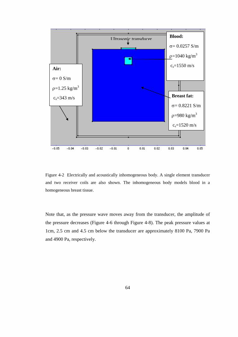
64
Figure 4-2 Electrically and acoustically inhomogeneous body. A single element transducer
and two receiver coils are also shown. The inhomogeneous body models blood in a
homogeneous breast tissue.
Note that, as the pressure wave moves away from the transducer, the amplitude of
the pressure decreases (Figure 4-6 through Figure 4-8). The peak pressure values at
1cm, 2.5 cm and 4.5 cm below the transducer are approximately 8100 Pa, 7900 Pa
and 4900 Pa, respectively.
Breast fat:
σ= 0.8221 S/m
ρ=980 kg/m3
cs=1520 m/s
Ultrasonic transducer Blood:
σ= 0.0257 S/m
ρ=1040 kg/m3
cs=1550 m/s
Air:
σ= 0 S/m
ρ=1.25 kg/m3
cs=343 m/s

65
Figure 4-3 Pressure distributions due to single element transducer for t = 0.1 µ in a
homogeneous body
Figure 4-4 Pressure distributions due to single element transducer for t = 10 µs in a
homogeneous body

66
Figure 4-5 Pressure distributions due to single element transducer for t = 25 µs in a
homogeneous body
Figure 4-6 Pressure waves in the homogeneous body at 1cm below the transducer along the
main axis of the transducer
0 0.5 1 1.5 2 2.5 3 3.5
x 10-5
-10000
-8000
-6000
-4000
-2000
0
2000
4000
Time (seconds)
Pres
sure
(Pa)

67
Figure 4-7 Pressure waves in the homogeneous body at 2.5 cm below the transducer along
the main axis of the transducer
Figure 4-8 Pressure waves in the homogeneous body at 4.5 cm below the transducer along
the main axis of the transducer
0 0.5 1 1.5 2 2.5 3 3.5
x 10-5
-8000
-6000
-4000
-2000
0
2000
4000
Time (seconds)
Pres
sure
(Pa)
0 0.5 1 1.5 2 2.5 3 3.5
x 10-5
-5000
-4000
-3000
-2000
-1000
0
1000
2000
3000
Time (seconds)
Pres
sure
(Pa)

68
Figure 4-9 Velocity current density distributions for t = 1 µs in the homogeneous body
Figure 4-10 Velocity current density distributions for t = 10 µs in the homogeneous body

69
Figure 4-11 Velocity current density distributions for t = 25 µs in the homogeneous
Figure 4-12 Pressure distributions generated with single element transducer for t = 0.1 µs in
inhomogeneous body (with blood)

70
Figure 4-13 Pressure distributions generated with single element transducer for t = 10 µs in
inhomogeneous body (with blood)
Figure 4-14 Pressure distributions generated with single element transducer for t = 25 µs in
inhomogeneous body (with blood)

71
Figure 4-15 Pressure waves in the inhomogeneous body at 1cm below the transducer along
the main axis of the transducer
Figure 4-16 Pressure waves in the inhomogeneous body at 2.5 cm below the transducer
along the main axis of the transducer
0 0.5 1 1.5 2 2.5 3 3.5
x 10-5
-10000
-8000
-6000
-4000
-2000
0
2000
4000
Time (seconds)
Pres
sure
(Pa)
0 0.5 1 1.5 2 2.5 3 3.5
x 10-5
-8000
-6000
-4000
-2000
0
2000
4000
Time (seconds)
Pres
sure
(Pa)

72
Figure 4-17 Pressure waves in the inhomogeneous body at 4.5 cm below the transducer
along the main axis of the transducer
Figure 4-15 through Figure 4-17 show the pressure distributions in inhomogeneous
body at 1 cm, 2.5 cm and 4.5 cm below the single element transducer. As the
pressure wave moves away from the transducer, the amplitude of the pressure wave
decreases. The peak pressure values at 1 cm, 2.5 cm and 4.5 cm below the transducer
are calculated as 8200 Pa, 7700 Pa and 5000 Pa, respectively.
In the inhomogeneous body (4 mm x 5 mm blood, 8 mm below the transducer), the
electrical conductivity of blood is higher compared to the breast fat (σblood = 0.8221
S/m, σbreast fat = 0.0257 S/m at 1MHz). Consequently, the induced current density in
the blood must be higher than the rest of the body (Figure 4-18 through Figure 4-20).
Note that the velocity current density induced in this domain must be under the
safety limit (Maximum induced current is about 5 mA/m2). In the homogeneous
domain maximum current is approximately 0.2 mA/m2 .
0 0.5 1 1.5 2 2.5 3 3.5
x 10-5
-5000
-4000
-3000
-2000
-1000
0
1000
2000
3000
Time (seconds)
Pres
sure
(Pa)

73
Figure 4-18 Velocity current density distributions for t= 0.1 µs in the inhomogeneous body
Figure 4-19 Velocity current density distributions for t= 3.6 µs in the inhomogeneous body
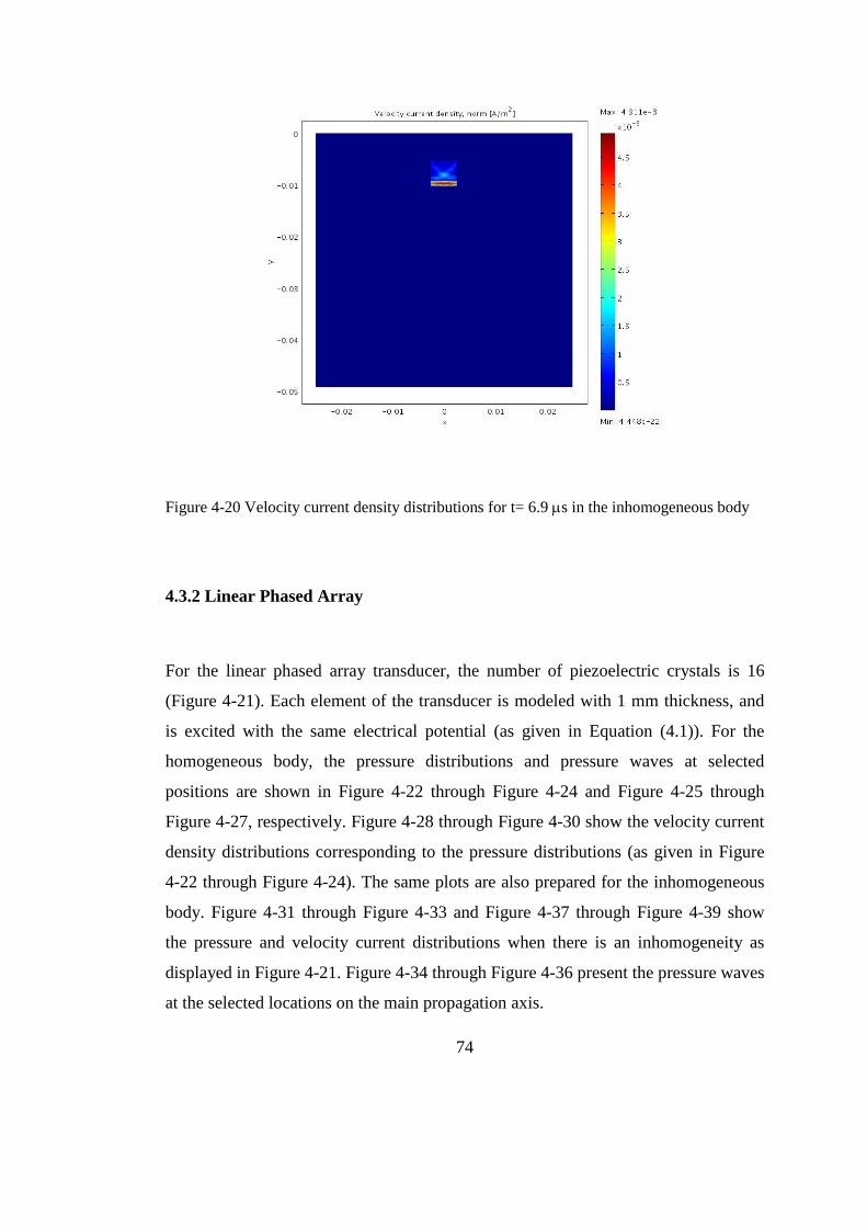
74
Figure 4-20 Velocity current density distributions for t= 6.9 µs in the inhomogeneous body
4.3.2 Linear Phased Array
For the linear phased array transducer, the number of piezoelectric crystals is 16
(Figure 4-21). Each element of the transducer is modeled with 1 mm thickness, and
is excited with the same electrical potential (as given in Equation (4.1)). For the
homogeneous body, the pressure distributions and pressure waves at selected
positions are shown in Figure 4-22 through Figure 4-24 and Figure 4-25 through
Figure 4-27, respectively. Figure 4-28 through Figure 4-30 show the velocity current
density distributions corresponding to the pressure distributions (as given in Figure
4-22 through Figure 4-24). The same plots are also prepared for the inhomogeneous
body. Figure 4-31 through Figure 4-33 and Figure 4-37 through Figure 4-39 show
the pressure and velocity current distributions when there is an inhomogeneity as
displayed in Figure 4-21. Figure 4-34 through Figure 4-36 present the pressure waves
at the selected locations on the main propagation axis.

75
For both cases (homogeneous and inhomogeneous) as the pressure wave moves away
from the transducer, the amplitude of the pressure decreases. The peak pressure
values at 1 cm, 2.5 cm and 4.5 cm are calculated as 3000 Pa, 2700 Pa and 2400 Pa
for the homogeneous body, respectively. For the inhomogeneous body, the peak
pressure values at the same positions are calculated as 3100 Pa, 2600 Pa and 2400 Pa,
respectively.
The velocity current density distributions show that the induced current in the blood
is under the safety limit (Maximum induced current density is about 2 mA/m2). In the
homogeneous body, however, maximum current density is even less, i.e., it is
approximately 0.1 mA/m2 .
Figure 4-21 Electrically and acoustically inhomogeneous body. A 16-element linear phased
array transducer and two receiver coils are also shown. The inhomogeneous body models
blood in a homogeneous breast tissue.
Breast fat:
σ= 0.8221 S/m
ρ=980 kg/m3
cs=1520 m/s
16-element linear phased array Blood:
σ=0.0257 S/m
ρ=1040 kg/m3
cs=1550 m/s
Air:
σ= 0 S/m
ρ=1.25 kg/m3
cs=343 m/s
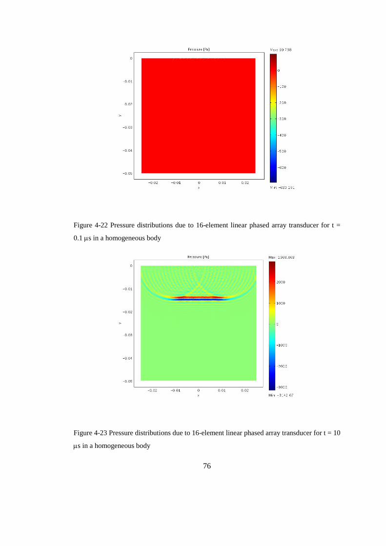
76
Figure 4-22 Pressure distributions due to 16-element linear phased array transducer for t =
0.1 µs in a homogeneous body
Figure 4-23 Pressure distributions due to 16-element linear phased array transducer for t = 10
µs in a homogeneous body

77
Figure 4-24 Pressure distributions due to 16-element linear phased array transducer for t = 25
µs in a homogeneous body
Figure 4-25 Pressure waves in the homogeneous body at 1 cm below the transducer along the
main axis of the transducer (16-element linear phased array)
0 0.5 1 1.5 2 2.5 3 3.5
x 10-5
-4000
-3000
-2000
-1000
0
1000
2000
3000
Time (seconds)
Pres
sure
(Pa)

78
Figure 4-26 Pressure waves in the homogeneous body at 2.5 cm below the transducer along
the main axis of the transducer (16-element linear phased array)
Figure 4-27 Pressure waves in the homogeneous body at 4.5 cm below the transducer along
the main axis of the transducer (16-element linear phased array)
0 0.5 1 1.5 2 2.5 3 3.5
x 10-5
-3000
-2000
-1000
0
1000
2000
3000
Time (seconds)
Pres
sure
(Pa)
0 0.5 1 1.5 2 2.5 3 3.5
x 10-5
-3000
-2000
-1000
0
1000
2000
Time (seconds)
Pres
sure
(Pa)

79
Figure 4-28 Velocity current density distributions for t = 0.1 µs in the homogeneous body
(16-element linear phased array transducer)
Figure 4-29 Velocity current density distributions for t =10 µs in the homogeneous body (16-
element linear phased array transducer)

80
Figure 4-30 Velocity current density distributions for t =25 µs in the homogeneous body (16-
element linear phased array transducer)
Figure 4-31Pressure distributions due to 16-element linear phased array transducer for t = 0.1
µs in the inhomogeneous body

81
Figure 4-32 Pressure distributions due to 16-element linear phased array transducer for t = 10
µs in the inhomogeneous body
Figure 4-33 Pressure distributions due to 16-element linear phased array transducer for t = 25
µs in the inhomogeneous body

82
Figure 4-34 Pressure waves in the inhomogeneous body at 1cm below the transducer along
the main axis of the transducer (16-element linear phased array)
Figure 4-35 Pressure waves in the inhomogeneous body at 2.5 cm below the transducer
along the main axis of the transducer (16-element linear phased array)
0 0.5 1 1.5 2 2.5 3 3.5
x 10-5
-3000
-2000
-1000
0
1000
2000
3000
Time (seconds)
Pres
sure
(Pa)
0 0.5 1 1.5 2 2.5 3 3.5
x 10-5
-3000
-2000
-1000
0
1000
2000
3000
Time (seconds)
Pres
sure
(Pa)

83
Figure 4-36 Pressure waves in the inhomogeneous body at 4.5 cm below the transducer
along the main axis of the transducer (16-element linear phased array)
Figure 4-37 Velocity current density distributions for t = 0.1 µs in the inhomogeneous body
0 0.5 1 1.5 2 2.5 3 3.5
x 10-5
-2500
-2000
-1500
-1000
-500
0
500
1000
1500
Time (seconds)
Pres
sure
(Pa)

84
Figure 4-38 Velocity current density distributions for t = 3.6 µs in the inhomogeneous body
Figure 4-39 Velocity current density distributions for t = 6.9 µs in the inhomogeneous body

85
4.4 Measurement of Induced Voltage along Receiver Coils
In order to measure the velocity current density induced in the conductive body and
tumor tissue, we use two receiver coils, namely, x-coil and y-coil. Detailed
information about the receiver coils is given in Chapter 3 Coil Configuration part.
These coils are encircling the conductive body. The induced voltages in the receiver
coils can be calculated using the following line integral:
𝑉𝑉𝑖𝑖𝑖𝑖𝑎𝑎 = −∫𝐸𝐸 𝑖𝑖𝑖𝑖𝑎𝑎 ∙ 𝑎𝑎𝐽𝐽 (4.3)
where 𝐸𝐸 𝑖𝑖𝑖𝑖𝑎𝑎 represents the electric field along the receiver coil geometry and 𝑎𝑎𝐽𝐽
denotes the differential element on the coil path. Note that, a different approach is
presented in Chapter 2 that expresses the measurements in terms of the lead-fields.
To verify the lead field formulation, the receiver voltages are calculated using the
two approaches: 1) using the lead field equation (Equation (2.101)) and 2) using the
line integral equation (Equation 4.3). For this comparison 16-element linear phased
array transducer is placed on the upper edge of the body. The steering angle is
chosen as zero degree.
Figure 4-40 shows the normalized voltage waveforms for the homogeneous body.
Figure 4-41 shows the normalized receiver voltages for the inhomogeneous body.
For both cases, the voltage waveforms obtained by the lead-field approach closely
follow the waveforms obtained by the line integral expression. Consequently, one
may conclude that the lead field approach correctly models the forward problem of
the proposed approach. The lead field formulation will be the basis of the inverse
problem studies presented in the latter sections.

86
a)
b)
Figure 4-40 Induced voltage along x-coil for homogeneous conductive body with 16-element
linear phased array transducer a) using Equation (4.3) b) using the lead field equation
(Equation (2.101))
0 0.5 1 1.5 2 2.5 3 3.5
x 10-5
-0.2
0
0.2
0.4
0.6
0.8
1
1.2Normalized Induced Voltage along the x-coil
time (seconds)
Nor
mal
ized
Indu
ced
Volta
ge (V
/V)
0 0.5 1 1.5 2 2.5 3 3.5
x 10-5
-0.2
0
0.2
0.4
0.6
0.8
1
1.2Normalized Induced Voltage Calculated with Lead Fields
time (seconds)
Nor
mal
ized
Indu
ced
Volta
ge (V
/V)

87
a)
b)
Figure 4-41 Induced voltage along x-coil for inhomogeneous conductive body ( blood is
placed 8 mm below the transducer, with 5 mm x 5mm geometry) with 16-element linear
phased array a) using Equation (4.3) b) using the lead fields (Equation (2.101))
0 0.5 1 1.5 2 2.5 3 3.5
x 10-5
-1
-0.5
0
0.5
1Normalized Induced Voltage along the x-coil
time (seconds)
Nor
mal
ized
Indu
ced
Volta
ge (V
/V)
0 0.5 1 1.5 2 2.5 3 3.5
x 10-5
-1.5
-1
-0.5
0
0.5
1Normalized Induced Voltage Calculated with Lead Fields
time (seconds)
Nor
mal
ized
Indu
ced
Volta
ge (V
/V)

88
4.5 Inverse Problem Solution
The aim of this imaging modality is to reconstruct the electrical impedance
distribution j (or its change relative to a known distribution). With
the proposed approach this can be achieved in two ways:
1) Time-Harmonic excitation: In this way, the ultrasonic transducer is excited
sinusoidally at its resonance frequency and a steady-state current distribution is
developed inside the body. The magnetic fields of the induced current can be
measured by detector coils placed nearby the body or by encircling coils. The
number of measurements can be increased by changing the transducer position.
Ww The relation between the pick-up voltages and conductivity
distribution in the body is already derived and given by equation (2.105):
𝑽(σ) = ∫𝜕
𝜕𝑡𝜎( × 𝟎) ∙ 𝑴(𝜎)𝑑𝑉
𝑉𝑏𝑜𝑑𝑦 (4.4)
where 𝑴 (the lead field vector) is the electric field in the reciprocal problem
when unit current is applied to the receiver coil.
The relation between the measurement and conductivity is a non-linear mapping.
However the first-order variation in the measurement related to conductivity
perturbation can be determined. The measurement for a known conductivity
distribution 𝜎0 can be written as
𝐕(σ0) = ∫𝜕
𝜕𝑡𝜎0( × 𝟎) ∙ 𝑴(𝜎0)𝑑𝑉
𝑉𝑏𝑜𝑑𝑦 (4.5)
Equation (4.5) can be rewritten when 𝜎 is replaced by 𝜎0 + ∆𝜎,

89
𝑽(σ0 + ∆𝜎) = ∫𝜕
𝜕𝑡(𝜎0 + ∆𝜎)( × 𝟎) ∙ 𝑴(𝜎0 + ∆𝜎)𝑑𝑉 (4.6)
𝑉𝑏𝑜𝑑𝑦
When we approximate 𝑴(𝜎) with the lead field of the initial conductivity
distribution, i.e., 𝑴(𝜎) ≅ 𝑴(𝜎0), then the following relation is valid,
𝑽(σ0 + ∆𝜎) − 𝐕(σ0) = ∫ ∆𝜎𝜕
𝜕𝑡( × 𝟎) ∙ 𝑴(𝜎0)𝑑𝑉 (4.7)
𝑉𝑏𝑜𝑑𝑦
A discretized version of Equation (4.7) can be written as
∆𝑉 = ∑ ( 𝑣𝑒𝑙 ∙ 𝑀)𝑁𝑗=1 ∆𝜎 (4.8)
where N represents the number of elements in the discrete conductivity model. By
changing the coil/transducer configuration it is possible to obtain M independent
measurements yielding the following matrix equation relating the change in
measurements to a perturbation in conductivity:
∆𝐕 = 𝑺𝑻𝑯 ∆𝛔 (4.9)
Here 𝑺𝑻𝑯 represents the sensitivity matrix for the time-harmonic excitation. In
this study, the performance of imaging using time-harmonic excitation is not studied
in detail, though the theory behind is clarified.
2) Pulse type excitation: When the transducer is excited with an electrical pulse,
then a pressure wave is generated inside the body. In such a case, the particle
velocity is a function of time, i.e., 𝑣 = 𝑣 (𝑡) yielding a velocity current density
distribution propagating inside the body. The relation between the pick-up voltage
and conductivity distribution will be very similar to the time-harmonic case as shown
by equation (2.101). However, the measurement in such a case is time varying:

90
𝑉(σ, t) = ∫ 𝜎( (t) × 𝟎) ∙ 𝑀(𝜎)𝑑𝑉 (4.10)𝑉𝑏𝑜𝑑𝑦
The first order variation in the measurements can now be written in the data
acquisition period (TD ) as,
𝑉(σ0 + ∆𝜎, 𝑡) − V(σ0, t) = ∫ ∆𝜎(𝑣 (t) × 0) ∙ 𝑀(𝜎0)𝑑𝑉 (4.11) 𝑉𝑏𝑜𝑑𝑦
The discretized version can be written as:
∆𝑉(𝑡) = ∑ ( 𝑣𝑒𝑙(𝑡) ∙ 𝑀)𝑁
𝑗=1∆𝜎 𝑡 < 𝑇𝐷 (4.12)
This relation can be written for M different time instants (∆𝑡 = 𝑇𝐷/𝑀) as follows:
∆𝑉(𝑖∆𝑡) = ∑ ( 𝑣𝑒𝑙(𝑖∆𝑡) ∙ 𝑀)𝑁
𝑗=1∆𝜎 𝑖 = 1…𝑀 (4.13)
Consequently, a matrix equation can be obtained for a specific transducer position
and coil configuration:
∆𝐕 = 𝑺𝑷 ∆𝛔 (4.14)
where 𝑺𝑷 represents the 𝑀 × 𝑁 sensitivity matrix for a pulse type excitation.
In this study, a novel receiver coil configuration is proposed which consists of an x-
coil and y-coil (Details are given in Chapter 2 and 3). As their name implies each coil
is more sensitive to the currents in the corresponding direction. To specify which coil
is used for the measurements an appropriate subscript (i.e., x or y) is added to the
relevant terms in equation (4.14) and pick-up voltages are written in the following
forms:
∆𝐕𝐱 = 𝑺𝑷𝒙 ∆𝛔 (4.15)
∆𝐕𝐲 = 𝑺𝑷𝒚 ∆𝛔 (4.16)

91
or a larger system of equations can be obtained as
∆𝐕𝐕𝐱𝐱∆𝐕𝐕𝐲𝐲
= 𝑺𝑺𝑷𝑷𝑷𝑷𝑺𝑺𝑷𝑷𝑷𝑷
∆𝛔𝛔 (4.17)
Equation (4.17) can also be written in the following form:
∆𝐕𝐕𝐱𝐱𝐲𝐲 = 𝑺𝑺𝑷𝑷𝑷𝑷𝑷𝑷 ∆𝛔𝛔 (4.18)
where 𝑺𝑺𝒑𝒑𝑷𝑷𝑷𝑷 is an 2MxN sensitivity matrix and ∆𝐕𝐕𝐱𝐱𝐲𝐲 is a 2Mx1 measurement vector.
Note that Equation (4.17) is written for a specific transducer position. It is always
possible to increase the number of measurements by changing the transducer location.
In this thesis study, to obtain the sensitivity matrix two electromagnetic problems are
solved. Firstly, electric fields are computed due to the reciprocal currents in the
receiver coils. Thereafter, electric fields (Lorentz Electric Fields) are computed due
to the excitation of the ultrasonic transducer in the main static magnetic field. The
dot product of the electric fields for each pixel gives the corresponding entries in the
sensitivity matrix.
To understand the characteristics of the imaging system, the sensitivity matrix must
be analyzed. For this purpose, the transducer-body-receiver coil configuration should
be specified. In this study, the body is chosen as 5 cm x 5 cm square object and it is
divided into 0.5 mm x 0.5 mm elements, yielding 10000 pixels (N =10000). As it is
mentioned in Section 4.2 (Transducer Excitation), the run-time for each simulation is
32.8µs with 0.1µs time intervals. Thus, for each simulation the number of
measurements (M) is 328. The linear phased array transducer is assumed to be
located at two positions, namely, the upper and the right edges of the body. For each
transducer position, the sensitivity matrix is calculated for seven steering angles (-
22.5°, -15°, -7.5°, 0°, 7.5°, 15°, 22.5°). Thus, the sensitivity matrix S is of dimension
9184x10000. Note that the number of measurements (NM) is obtained using the
following formula:

92
𝑁𝑁𝑀𝑀 = 𝑁𝑁𝑆𝑆𝑇𝑇 × 𝑁𝑁𝑇𝑇𝑃𝑃 × 𝑁𝑁𝑅𝑅𝐶𝐶 × 𝑁𝑁𝑆𝑆𝐸𝐸
where
NST: number of steering angles for each transducer position,
NTP: number of transducer positions,
NRC: number of receiver coils,
NSE: number of samples for each excitation.
To get insight about the characteristics of the sensitivity matrix, a specific row is
displayed for a 16-element linear phased array transducer. Figure 4-42 shows the
problem geometry used for the sensitivity calculations. In this study, the steering
angle 0° is chosen, i.e., the pressure wave is propagating in the main axis (y-axis) of
the transducer. Since the resultant velocity field is in x-direction, the sensitivity
profile obtained for the x-coil is analyzed. The Lorentz field is calculated at t=10 𝜇𝜇s
and shown in Figure 4-43. Figure 4-44 shows the electric field distribution inside the
body due to a unit reciprocal current in the x-coil. The corresponding row of the
sensitivity matrix is shown in Figure 4-45.

93
Figure 4-42 A linear 16 element phased- array transducer positioned at the upper boundary
of the body. The geometry of the receiver coil (x-coil) is also shown.
Figure 4-43 Lorentz electric field (V/m) distribution at t = 10 µs due to 16-element linear
phased array transducer.
x
y
Lorentz Electric Field Distribution
-0.02 -0.01 0 0.01 0.02-0.05
-0.045
-0.04
-0.035
-0.03
-0.025
-0.02
-0.015
-0.01
-0.005
0
-1.5
-1
-0.5
0
0.5
1
1.5
2x 10⁻³
16-element linear phased array transducer
breast fat
x-coil
air

94
Figure 4-44 Electric field (V/m) distribution induced by the reciprocal current in the x-coil.
Figure 4-45 Image of the sensitivity (Vm/S) pattern for the selected transducer-coil
configuration (as shown in Figure 4-42) at t = 10 s.
x
y
-0.02 -0.01 0 0.01 0.02-0.05
-0.045
-0.04
-0.035
-0.03
-0.025
-0.02
-0.015
-0.01
-0.005
0
-4
-2
0
2
4
6
x 10-10

95
Figure 4-46 One-dimensional plot of the sensitivity (V⋅m/S) distribution for the specific
transducer-coil configuration (Figure 4-42) at time instant t = 10 µs.
To understand the performance of the imaging system, the sensitivity matrix is
analyzed using the Singular Value Decomposition (SVD). SVD of a matrix A is
given as:
𝑨𝑨 = 𝑼𝑼𝑺𝑺𝑽𝑽𝑻𝑻 (4.9)
where U and V matrices are orthonormal matrices. The columns of U and V are the
left-singular vectors and right-singular vectors of A, respectively. S is a diagonal
matrix whose diagonal entries (the singular values of A) are arranged in the order of
decreasing magnitude. The resolution matrix [47] calculated as,
R=VVT (4.10)
0 2000 4000 6000 8000 10000-6
-4
-2
0
2
4
6
8x 10⁻¹⁰
number of pixels

96
is usually used to test the resolution properties of a linear imaging system. If n is the
number of pixels in the imaging domain, then R is an nxn matrix. Note that each
column or row of the resolution matrix shows the reconstructed image due to a single
pixel perturbation. If the number of right singular vectors is equal to the number of
unknowns, then R becomes an identity matrix (showing identical reconstruction for
each perturbation). However, if there is noise in the measurements, some singular
vectors corresponding to small singular values must be truncated. This yields a
reduction in the number of image basis vectors used in image reconstruction and R
differs from the identity matrix (Appendix C).
The resolution matrix of the proposed system is calculated assuming an SNR of
80dB. This results in limited number of basis vectors (5648) to be used in the
calculation of the resolution matrix. Figure 4-47 shows a specific part of the
10000x10000 resolution matrix under this condition. The diagonal characteristic of
the resolution matrix is evident; however, the magnitudes differ depending on the
pixel position.
The resolution matrix can be further analyzed by generating the so-called resolution
map of the imaging system. This map is formed using only the diagonal elements of
the resolution matrix which usually represent the peak response of the system to
single pixel perturbations. Figure 4-48 shows the resolution map of the generated
10000x10000 resolution matrix. It is clearly seen that the proposed imaging
configuration has higher sensitivity to pixels under the transducers and has lower
sensitivity to pixels away from both transducer locations. The maximum steering
angle (22.5°) is also effective in this response.
Figure 4-49 shows the singular values of the sensitivity matrix normalized with the
maximum singular value. The condition number is calculated as 3.29 x10⁷.

97
Figure 4-47 A specific portion of the resolution matrix (10000x10000) corresponding to the
proposed transducer-receiver coil configuration. The receiver coils record data for a period
of 32.8µs with 0.1µs sampling intervals. The transducer is located at two positions, namely,
the upper and the left edges of the body. For each transducer position, the sensitivity matrix
is calculated for seven steering angles (-22.5°, -15°, -7.5°, 0°, 7.5°, 15°, 22.5°).

98
Figure 4-48 Resolution map of the 10000x10000 resolution matrix (SNR 80 dB)
Figure 4-49 Normalized singular values of the sensitivity matrix
0 2000 4000 6000 8000 1000010
-25
10-20
10-15
10-10
10-5
100
index(i)

99
4.6 Image Reconstruction
In this thesis study, the Truncated SVD method is used to reconstruct the images of
the conductivity distribution. If the resolution matrix R is an identity matrix, any
perturbation in the imaging domain can be identically reconstructed. However, due to
the noise level in the measurements the number of image basis vectors used in image
reconstruction may change (Appendix C). If the number of image basis vectors (𝑟𝑟) is
less than 𝑖𝑖 , then V will be 𝑖𝑖 × 𝑟𝑟 matrix. Consequently, the characteristics of
resolution matrix R will change according to the number of truncated basis vectors.
The performance of the proposed imaging system can be assessed by simulation
studies. For this purpose, two body models are prepared:
a) Model 1: A single inhomogeneity (square domain of conductivity 0.8221
S/m) located at the center of the body (at a distance of 2.5 cm from the
transducers) (Figure 4-50 and Figure 4-51).
b) Model 2: Five identical inhomegeneities (square domain of conductivity
0.8221 S/m) located symmetrically in the imaging domain. One is at the
center of the body; others are at 1 cm distance from the body surfaces (Figure
4-52 and Figure 4-53).
Initially, a single transducer (16 –element linear phased array) is used for excitation
as shown in Figure 4-26. The sensitivity matrix is calculated for seven steering
angles (-22.5°, -15°, -7.5°, 0°, 7.5°, 15°, 22.5°). Thus, the sensitivity matrix SPx is of
dimension 4592x10000.To assess the reconstruction performance in the case of noisy
data Gaussian noise is added to the measurements. Images of the first model (Model
1) are reconstructed according to the SNRs of 20dB, 40 dB, 80 dB and with
maximum SNR. Figures 4-54 through Figure 4-57 present the reconstructed images.
The number of basis vectors used for different SNRs is given in Table 4-1. The

100
resolution in the images increases as the SNR in the measurements increases. It is
observed that SNR is more demanding to improve resolution in y-direction whereas
the resolution in x direction is high even at the lowest SNR in the measurements.
One dimensional plots (Figures 4-58 through Figure 4-61) of the reconstructed
conductivities (along x=0 line) shows that behavior more clearly.
To equalize the resolution in both directions, data is acquired for a second transducer
position (Figure 4-51). Thus the number of measurements is doubled. The resultant
sensitivity matrix SPxy is of dimension 9184x10000. Figure 4-62 through Figure 4-65
are the reconstructed images of Model 1. The number of basis vectors used for
different SNRs is given in Table 4-2. One dimensional plots (Figures 4-66 through
Figure 4-69) of the reconstructed conductivities (along x=0 line) shows the
improvement in resolution.
Table 4-1Number of basis vectors for different SNRs. Single transducer excitation.
SNR (dB) Number of basis vectors 20 783 40 1509 80 3051 137 (max) 4500
Table 4-2 Number of basis vectors for different SNRs. Two transducer excitations.
SNR (dB) Number of basis vectors 20 1453 40 2821 80 5641 182 (max) 9100

101
Figure 4-70 through Figure 4-73 are the reconstructed images of Model 2. As
expected, the resolution in the reconstructed images improves as the SNR in the
measurement increases. A notable feature of the system is that even an SNR of 20dB
yields images that show the positions and sizes of the objects correctly.
Figure 4-50 A single inhomogeneity (square domain of conductivity 0.8221 S/m ) is
located at the center of the body (Model 1). The transducer is placed is on the top
side of the conductive body.
air
16-element linear phased array
blood
breast fat

102
Figure 4-51 A single inhomogeneity (square domain of conductivity 0.8221 S/m) is located
at the center of the body (Model 1). The transducer is placed is on the left side of the
conductive body.
Figure 4-52 Five identical inhomegeneities (square domain of conductivity 0.8221 S/m )
located symmetrically in the imaging domain (Model 2). The transducer is placed is on the
top side of the conductive body.
blood
breast fat
air 16-e
lem
ent l
inea
r p
hase
d ar
ray
16-element linear phased array
blood
blood blood blood
blood
breast fat
air

103
Figure 4-53 Five identical inhomegeneities (square domain of conductivity 0.8221 S/m) are
located symmetrically in the imaging domain (Model 2). The transducer is placed is on the
left side of the conductive body.
Figure 4-54 The reconstructed image of Model 1 when the SNR is 20 dB. Data is acquired
using a single transducer located on the top edge of the body.
x
y
-0.02 -0.01 0 0.01 0.02-0.05
-0.045
-0.04
-0.035
-0.03
-0.025
-0.02
-0.015
-0.01
-0.005
0
-0.3
-0.2
-0.1
0
0.1
0.2
0.3
0.4
0.5
16-e
lem
ent l
inea
r pha
sed
arra
y
blood
blood blood blood
blood
breast fat
air

104
Figure 4-55 The reconstructed image of Model 1 when the SNR is 40 dB. Data is acquired
using a single transducer located on the top edge of the body
Figure 4-56 The reconstructed image of Model 1 when the SNR is 80 dB. Data is acquired
using a single transducer located on the top edge of the body.
x
y
-0.02 -0.01 0 0.01 0.02-0.05
-0.045
-0.04
-0.035
-0.03
-0.025
-0.02
-0.015
-0.01
-0.005
0
-0.2
-0.1
0
0.1
0.2
0.3
0.4
0.5
0.6
0.7
x
y
-0.02 -0.01 0 0.01 0.02-0.05
-0.045
-0.04
-0.035
-0.03
-0.025
-0.02
-0.015
-0.01
-0.005
0
-0.1
0
0.1
0.2
0.3
0.4
0.5
0.6
0.7
0.8

105
Figure 4-57 The reconstructed image of Model 1 when the SNR is maximum. Data is
acquired using a single transducer located on the top edge of the body.
Figure 4-58 One-dimensional plot of the reconstructed conductivities (Figure 4-54) along
x=0 line. SNR = 20dB.
x
y
-0.02 -0.01 0 0.01 0.02-0.05
-0.045
-0.04
-0.035
-0.03
-0.025
-0.02
-0.015
-0.01
-0.005
0
-0.1
0
0.1
0.2
0.3
0.4
0.5
0.6
0.7
0.8
0 10 20 30 40 50 60 70 80 90 100-0.05
0
0.05
0.1
0.15
0.2
0.25
0.3
0.35
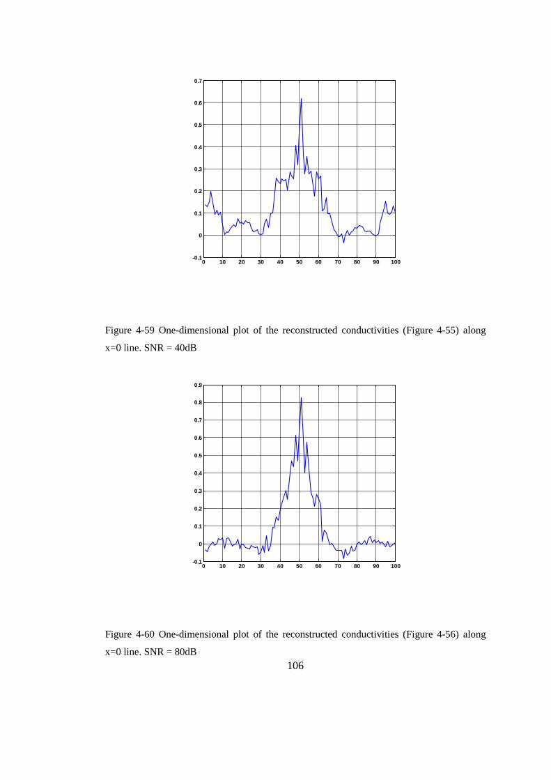
106
Figure 4-59 One-dimensional plot of the reconstructed conductivities (Figure 4-55) along
x=0 line. SNR = 40dB
Figure 4-60 One-dimensional plot of the reconstructed conductivities (Figure 4-56) along
x=0 line. SNR = 80dB
0 10 20 30 40 50 60 70 80 90 100-0.1
0
0.1
0.2
0.3
0.4
0.5
0.6
0.7
0 10 20 30 40 50 60 70 80 90 100-0.1
0
0.1
0.2
0.3
0.4
0.5
0.6
0.7
0.8
0.9

107
Figure 4-61 One-dimensional plot of the reconstructed conductivities (Figure 4-57) along
x=0 line. SNR = 182dB
Figure 4-62 The reconstructed image of Model 1 when the SNR is 20 dB. Data is acquired
using two transducer positions.
0 10 20 30 40 50 60 70 80 90 100-0.1
0
0.1
0.2
0.3
0.4
0.5
0.6
0.7
0.8
0.9
x
y
-0.02 -0.01 0 0.01 0.02-0.05
-0.045
-0.04
-0.035
-0.03
-0.025
-0.02
-0.015
-0.01
-0.005
0
-0.2
-0.1
0
0.1
0.2
0.3
0.4
0.5
0.6
0.7

108
Figure 4-63 The reconstructed image of Model 1 when the SNR is 40 dB. Data is acquired
using two transducer positions.
Figure 4-64 The reconstructed image of Model 1 when the SNR is 80 dB. Data is acquired
using two transducer positions.
x
y
-0.02 -0.01 0 0.01 0.02-0.05
-0.045
-0.04
-0.035
-0.03
-0.025
-0.02
-0.015
-0.01
-0.005
0
-0.1
0
0.1
0.2
0.3
0.4
0.5
0.6
0.7
0.8
x
y
-0.02 -0.01 0 0.01 0.02-0.05
-0.045
-0.04
-0.035
-0.03
-0.025
-0.02
-0.015
-0.01
-0.005
0
0
0.1
0.2
0.3
0.4
0.5
0.6
0.7
0.8

109
Figure 4-65 The reconstructed image of Model 1 when the SNR is 182 dB. Data is acquired
using two transducer positions.
Figure 4-66 One-dimensional plot of the reconstructed conductivities (Figure 4-62) along
x=0 line. SNR = 20dB.
x
y
-0.02 -0.01 0 0.01 0.02-0.05
-0.045
-0.04
-0.035
-0.03
-0.025
-0.02
-0.015
-0.01
-0.005
0
0
0.1
0.2
0.3
0.4
0.5
0.6
0.7
0 10 20 30 40 50 60 70 80 90 100-0.2
-0.1
0
0.1
0.2
0.3
0.4
0.5
0.6
0.7
0.8

110
Figure 4-67 One-dimensional plot of the reconstructed conductivities (Figure 4-63) along
x=0 line. SNR = 40dB.
Figure 4-68 One-dimensional plot of the reconstructed conductivities (Figure 4-64) along
x=0 line. SNR = 80dB.
0 10 20 30 40 50 60 70 80 90 100-0.1
0
0.1
0.2
0.3
0.4
0.5
0.6
0.7
0.8
0.9
0 10 20 30 40 50 60 70 80 90 100-0.1
0
0.1
0.2
0.3
0.4
0.5
0.6
0.7
0.8
0.9

111
Figure 4-69 One-dimensional plot of the reconstructed conductivities (Figure 4-65) along
x=0 line. SNR = 182dB.
Figure 4-70 The reconstructed image of Model 2 when the SNR is 20 dB. Data is acquired
using two transducer positions.
0 10 20 30 40 50 60 70 80 90 100-0.1
0
0.1
0.2
0.3
0.4
0.5
0.6
0.7
0.8
x
y
-0.02 -0.01 0 0.01 0.02-0.05
-0.045
-0.04
-0.035
-0.03
-0.025
-0.02
-0.015
-0.01
-0.005
0
-0.4
-0.2
0
0.2
0.4
0.6
0.8

112
Figure 4-71 The reconstructed image of Model 2 when the SNR is 40 dB. Data is acquired
using two transducer positions.
Figure 4-72 The reconstructed image of Model 2 when the SNR is 80 dB. Data is acquired
using two transducer positions.
x
y
-0.02 -0.01 0 0.01 0.02-0.05
-0.045
-0.04
-0.035
-0.03
-0.025
-0.02
-0.015
-0.01
-0.005
0
-0.6
-0.4
-0.2
0
0.2
0.4
0.6
0.8
x
y
-0.02 -0.01 0 0.01 0.02-0.05
-0.045
-0.04
-0.035
-0.03
-0.025
-0.02
-0.015
-0.01
-0.005
0
0
0.2
0.4
0.6
0.8
1

113
Figure 4-73 The reconstructed image of Model 2 when the SNR is 80 dB. Data is
acquired using two transducer positions.
x
y
-0.02 -0.01 0 0.01 0.02-0.05
-0.045
-0.04
-0.035
-0.03
-0.025
-0.02
-0.015
-0.01
-0.005
0
0
0.1
0.2
0.3
0.4
0.5
0.6
0.7
0.8

114
CHAPTER 5
CONCLUSION AND DISCUSSION
In this study a new imaging modality is proposed to image electrical conductivity of
body tissues. This modality is based on the magnetic field measurements generated
by ultrasonically induced Lorentz fields. The magnetic fields are measured using two
coils encircling the body. The two coil configurations (x- and y-coils) are designed to
be sensitive to currents in x- and y- directions, respectively. The properties of the
proposed approach are revealed by exploiting the multiphysics characteristics
(acoustic, piezoelectric, and electromagnetic) involved in its different phases. Basic
field equations governing the behavior of the time-varying acoustic and
electromagnetic fields are reviewed. The relation between the measurements and
conductivity distribution is derived. The resulting formulation is linearized around an
initial conductivity distribution. The characteristics of the imaging system are studied
by analyzing the sensitivity matrix using the SVD. The performance of the imaging
system is investigated using simulation studies.
This proposed imaging modality is based on the results reported for Hall Effect
Imaging [48]. Since the theory and basic assumptions behind the forward problem of
Hall Effect Imaging was not discussed elsewhere, the initial phase of this thesis study
is to reveal the corresponding theory. Thereafter, the forward problem of the
proposed approach is described. Magnetic fields of the induced velocity current
propagation and their relation to body conductivity distributions are explained. The
lead field analyses are described for the new measurement system for two different

115
excitations, namely, the time harmonic excitation, and pulse type excitations. The
imaging performance for the pulse-type excitations are discussed in detail. The
results show the potent of this new imaging modality.
Comments and discussions on different phases of this study are listed below.
Numerical Modeling: The characteristics of the forward problem are analyzed using
finite element based commercial software (Comsol Multiphysics). In the numerical
modeling, the pressure acoustic, piezoelectric and electromagnetic modules are
coupled whenever it is necessary in the solution of the forward problem. In the
piezoelectric module, a single element transducer and 16-element linear phased array
transducer are modeled with PZT-5H material. Inverse piezoelectric effect is
performed by exciting each transducer with time-varying electrical potentials. In this
study, the transducers are excited with a sinusoidal potential of one cycle. The
piezoelectric crystals can be excited with longer sinusoidal potentials or tone burst
potentials that may yield different characteristics in the imaging system.
In the pressure acoustic module, the acoustic properties of the homogeneous and
inhomogeneous regions are modeled with the two major tissues in the breast (i.e.,
breast fat and breast fat with blood). The pressure generated in the body should be
originated from a pressure source. In this study, the outputs of the piezoelectric
module are assumed as the primary pressure source. The interaction of the velocity
currents with the static magnetic field is also taken into account as an acoustic dipole
source to the pressure module. In this study, the acoustic fields of crystals with a
resonance frequency of 1 MHz are considered. The acoustic behavior and
corresponding effects in the image reconstruction performance must be investigated
for different excitation frequencies.
In this study, only two-dimensional numerical models are used. The performance of
the system must be further investigated using three-dimensional models.
Receiver coil design: A novel coil configuration is proposed to detect the
ultrasonically induced Lorentz fields. This coil configuration is consisting of two

116
coils (x- and y-coils). A better coil (or even a dipole antenna) can be designed to
improve the system properties.
Note that, once the excitation is known, by simply analyzing the induced voltages in
the receiver coils, one can have an insight about the inhomogeneity inside the bodies.
Specific coils can be designed to follow the conductivity changes on a specific line.
Time gated amplification can be employed to remove the attenuation affects with
depth.
Sensitivity Matrix Analysis: The geometry and location of the transducer and
receiver coils are important parameters in sensing the inhomogeneity in the body. In
this study, a 16-element linear phased array transducer is assumed on the upper edge
of the conductive body. To improve the sensitivity, the transducer is also placed on
the left edge. The receiver coils are placed encircling the body and transducer. The
characteristics of the system are revealed by analyzing the sensitivity matrix and
resolution maps. It is observed that the proposed system has higher sensitivity under
the transducer and around the center of body; however, it has lower sensitivity
around the corners. The developed analysis tools must be employed to design a better
transducer/coil configuration that yields homogeneous sensitivity to the conductivity
perturbations.
Image Reconstruction: In this thesis study, the mathematical basis of a new
imaging modality is presented. To reconstruct the conductivity images only a single
algorithm, namely, the Truncated SVD is used. The performance of other
reconstruction algorithms must be further investigated.
To develop a more practical and faster imaging system, techniques must be
developed to reconstruct images without using matrix inversions.
Safety considerations: Precautions should be taken by keeping the excitation
potential of ultrasound transducers below a threshold in order not to cause
destructive heating. Ultrasonic transducers used for diagnostic purposes do not cause
destructive heating in the human body [49]. The ultrasonic transducers used in our

117
simulations are excited with amplitude of 1V at 1 MHz frequency and definitely do
not cause any harm to the body tissues.
The induced current density in the body should also be under the safety limits. In our
simulations the induced velocity current densities are approximately 0.2 mA/m2 and
5 mA/m2 for homogeneous and inhomogeneous body, respectively. These current
densities are below the safety limits at 1 MHz [50].
Future Work: The following topics can be further investigated:
• Time-harmonic imaging and corresponding coil configurations.
• The effects of the number of steering angles on the image resolution.
• The focusing property of the linear phased array transducers.
• The use of the proposed approach employing other ultrasonic transducers (see
Appendix A).
• The use of multi-frequency excitations.
• Three-dimensional simulations for different transducer types and for different
perturbations.
• Data acquisition system design for time-harmonic and pulse excitations.
• Experimental studies conducted using phantoms and animals and research on
clinical applications.
• In this study, the beam steering properties of linear phased array transducers
are employed to steer electrical currents inside a conductive body. The
methodology can be further extended to obtain magnetic field measurements
inside the body using Magnetic Resonance Imaging systems. This will
definitely improve the resolution in the resultant conductivity images.

118
REFERENCES
[1] Foster KR. Dielectric Properties of Tissues. The Biomedical Engineering
Handbook: Second Edition, vol. 89. CRC Press, 2000.
[2] Peters MJ, Stinstra JG, Hendriks M. Estimation of the electrical conductivity
of human tissue. Electromagnetics 2001;21:545.
[3] Chauveau N, Ayeva B, Rigaud B, Morucci JP. A multifrequency serial EIT
system. Physiological Measurement 1996;17:A7.
[4] Fedorowski A, Steciwko A. Biological effects of non-ionizing
electromagnetic radiation. Med. Pr., 1998.
[5] Barber DC, Brown BH. Applied Potential Tomography. Journal of Physics E-
Scientific Instruments 1984;17:723.
[6] Paulson K, Lionheart W, Pidcock M. Optimal Experiments In Electrical-
Impedance Tomography. Ieee Transactions on Medical Imaging 1993;12:681.

119
[7] Metherall P, Barber DC, Smallwood RH, Brown BH. Three-dimensional
electrical impedance tomography. Nature 1996;380:509.
[8] Gencer NG. Electrical impedance tomography using induced currents.
Electrical and Electronics Engineering, vol. Ph.D.: Middle East Technical University,
1993.
[9] Gencer NG, Kuzuoglu M, Ider YZ. Electrical-Impedance Tomography Using
Induced Currents. Ieee Transactions on Medical Imaging 1994;13:338.
[10] Freeston IL, Tozer RC. Impedance Imaging Using Induced Currents.
Physiological Measurement 1995;16:A257.
[11] Brandstatter B, Hollaus K, Hutten H, Mayer M, Merwa R, Scharfetter H.
Direct estimation of Cole parameters in multifrequency EIT using a regularized
Gauss-Newton method. Physiological Measurement 2003;24:437.
[12] Fitzgerald AJ, Thomas BJ, Cornish BH, Michael GJ, Ward LC. Extraction of
electrical characteristics from pixels of multifrequency EIT images. Physiological
Measurement 1997;18:107.
[13] Hampshire AR, Smallwood RH, Brown BH, Primhak RA. Multifrequency
And Parametric Eit Images Of Neonatal Lungs. Physiological Measurement
1995;16:A175.

120
[14] Mayer M, Brunner P, Merwa R, Smolle-Juttner FM, Maier A, Scharfetter H.
Direct reconstruction of tissue parameters from differential multifrequency EIT in
vivo. Physiological Measurement 2006;27:S93.
[15] Zhang S, Xu G, Wu H, Geng D, Yan W. Multi-frequency EIT Hardware
System Based on DSP.
[16] Scott GC, Joy MLG, Armstrong RL, Henkelman RM. Sensitivity Of
Magnetic-Resonance Current-Density Imaging. Journal of Magnetic Resonance
1992;97:235.
[17] Scott GC, Joy MLG, Armstrong RL, Henkelman RM. Measurement Of
Nonuniform Current-Density By Magnetic-Resonance. Ieee Transactions on Medical
Imaging 1991;10:362.
[18] Joy M, Scott G, Henkelman M. Invivo Detection Of Applied Electric
Currents By Magnetic-Resonance Imaging. Magnetic Resonance Imaging 1989;7:89.
[19] Zhang N. Electrical impedance tomography based on current density imaging.
Electrical Engineering, vol. MS: University of Toronto, 1992.
[20] Gao N, He B. Noninvasive imaging of bioimpedance distribution by means of
current reconstruction magnetic resonance electrical impedance tomography. Ieee
Transactions on Biomedical Engineering 2008;55:1530.

121
[21] Ider YZ, Onart S. Algebraic reconstruction for 3D magnetic resonance-
electrical impedance tomography (MREIT) using one component of magnetic flux
density. Physiological Measurement 2004;25:281.
[22] Kwon O, Woo EJ, Yoon JR, Seo JK. Magnetic resonance electrical
impedance tomography (MREIT): Simulation study of J-substitution algorithm. Ieee
Transactions on Biomedical Engineering 2002;49:160.
[23] S A-Z, D G, G L, Z YZ, J PA, S BM. A feasibility study of electromagnetic
induction tomography. 9th Int Conf On Electrical Bio-Impedance. Heidelberg, 1995.
p.426.
[24] Al-Zeibak S, Goss D, Lyon G, Yu ZZ, Peyton AJ, Beck MS. A feasibility
study of electromagnetic induction tomography. 9th Int Conf On Electrical Bio-
Impedance. Heidelberg, 1995. p.426.
[25] Gencer NG, Tek N. Imaging Tissue Conductivity via Contactless
Measuremens: A Feasibility Study. vol. 6(3). Turkish Journal of Electrical
Engineering ELEKTRIK, 1998. p.167.
[26] Griffiths H. Magnetic induction tomography. Measurement Science &
Technology 2001;12:1126.

122
[27] Towe BC, Islam MR. A Magnetoacoustic Method For The Noninvasive
Measurement Of Bioelectric Currents. Ieee Transactions on Biomedical Engineering
1988;35:892.
[28] Roth BJ, Basser PJ, Wikswo JP. A Theoretical-Model For Magnetoacoustic
Imaging Of Bioelectric Currents. Ieee Transactions on Biomedical Engineering
1994;41:723.
[29] Roth BJ, Wikswo JP. Comments on "Hall effect imaging". Ieee Transactions
on Biomedical Engineering 1998;45:1294.
[30] Xu Y, He B. Magnetoacoustic tomography with magnetic induction (MAT-
MI). Physics in Medicine and Biology 2005;50:5175.
[31] Li X, Xu Y, He B. Magnetoacoustic tomography with magnetic induction for
imaging electrical impedance of biological tissue. Journal of Applied Physics
2006;99.
[32] Xia RM, Li X, He B, Ieee. Magnetoacoustic tomography of biological tissue
with magnetic induction, 2007.
[33] Brinker K, Roth BJ. The effect of electrical anisotropy during
magnetoacoustic tomography with magnetic induction. Ieee Transactions on
Biomedical Engineering 2008;55:1637.

123
[34] Webb AG. Introduction to Biomedical Imaging, 2002.
[35] Erikson KR, Fry FJ, Jones JP. Ultrasound In Medicine - Review. Ieee
Transactions on Sonics and Ultrasonics 1974;SU21:144.
[36] Wells PNT. Biomedical Ultrasonics. London: Academic Press, 1977.
[37] Plonsey R, Collin R. Principles and Applications of Electromagnetic Fields.
NewYork: Mc.Graw-Hill, 1961.
[38] Gabriel C, Gabriel S, Corthout E. The dielectric properties of biological
tissues .1. Literature survey. Physics in Medicine and Biology 1996;41:2231.
[39] Gabriel S, Lau RW, Gabriel C. The dielectric properties of biological
tissues .2. Measurements in the frequency range 10 Hz to 20 GHz. Physics in
Medicine and Biology 1996;41:2251.
[40] Gabriel S, Lau RW, Gabriel C. The dielectric properties of biological
tissues .3. Parametric models for the dielectric spectrum of tissues. Physics in
Medicine and Biology 1996;41:2271.
[41] Cheng DK. Fundamentals of Engineering Electromagnetics, 1993.

124
[42] Carley M. Some Notes on Acoustics. 2001.
[43] Zielinski TG. Fundamentals of multiphysics modelling of piezo-poro-elastic
structures. Archives of Mechanics 2010;62:343.
[44] Comsol Help.
[45] Mortarelli JR. A Generalization Of The Geselowitz Relationship Useful In
Impedance Plethysmographic Field Calculations. Ieee Transactions on Biomedical
Engineering 1980;27:665.
[46] Cheo BR. A Reciprocity Theorem For Electromagnetic Fields With General
Time Dependence. Ieee Transactions on Antennas and Propagation 1965;AP13:278.
[47] Gencer NG, Tek MN. Electrical conductivity imaging via contactless
measurements. Ieee Transactions on Medical Imaging 1999;18:617.
[48] Wen H, Shah J, Balaban RS. Hall effect imaging. Ieee Transactions on
Biomedical Engineering 1998;45:119.
[49] Azhari H. Basics of Biomedical Ultrasounds for Engineers: A John Wiley &
Sons , Inc., Publication, 2010.

125
[50] Lionheart WRB, Kaipio J, McLeod CN. Generalized optimal current patterns
and electrical safety in EIT. Physiological Measurement 2001;22:85.
[51] Curie P, Curie J. Development par pression de l'elctricite polaire dans les
cristaux hemiedres a faces encliness. Comp Rend, 1980.
[52] Goldberg RL, Smith SW, Moottley JG, Ferrara KW. Ultrasound. In: Mudry
KM, Plonsey R, Bronzino JD, editors. Principles and Applications in Engineering
Series- Biomedical Imaging. 2003.
[53] Allen JL. Array antennas: New applications for an old technique. IEEE Spect,
vol. 1, 1964.
[54] Bobber RJ. Underwater Electroacoustic Measurements. Washington: Naval
Reseach Laboratory, 1970.
[55] Somer JC. Electronic Sector Scanning For Ultrasonic Diagnosis. Ultrasonics
1968;6:153.
[56] Vonramm OT, Thurstone FL. Cardiac Imaging Using A Phased-Array
Ultrasound System .1. System-Design. Circulation 1976;53:258.

126
[57] Goss SA, Johnston RL, Dunn F. Comprehensive Compilation Of Empirical
Ultrasonic Properties Of Mammalian-Tissues. Journal of the Acoustical Society of
America 1978;64:423.

127
APPENDIX A
ULTRASONIC TRANSDUCERS
A.1 Transducers
The acoustic waves can be generated in many ways. These waves are induced by
converting magnetic, thermal and electrical energy into mechanical energy. In
medical applications of ultrasound the piezoelectric effect plays a key role in several
techniques. Piezoelectric effect was first introduced in 1880 [51] which implies that
applying a stress to the quartz crystal causes an electrical potential across opposite
face of the material. In addition, the inverse event was observed, which shows
applying an electric field across the crystal could result in mechanical deformation.
By the leading of this innovation, many significant advances have been observed in
ultrasound imaging. As one of these advances we can mention to the development of
linear-array transducers. At first, transducer was moving manually to the region of
interest, which had taken many seconds. In this approach, only static objects could be
scanned. As a result of fast scanning, moving objects can also be scanned for real-
time imaging. For this purpose, researchers developed different types of ultrasound
transducers which steer the acoustic beam, rapidly. Some of them can steer the beam
mechanically, and some other can steer and focus electronically. Linear phased array
transducers are the ones that can steer and focus the beam electronically [52].

128
A.1.1 Transducer Materials- PZT
The ferroelectric materials are the well-known materials in medical ultrasound to
exhibit the piezoelectric effect. Having low intrinsic losses and high
electromechanical conversion efficiency makes a ferroelectric material called
ceramic lead zirconate-titanate (PZT), a proper choice as a standard transducer
material for medical ultrasound [52] . In Table A-1 the properties of linear array
elements made of PZT are shown.
Table A-1 Material Properties of Linear-Array Elements Made of PZT-5H [52]
Parameter Symbol Value Units
Density ρ 7500 kg/m3
Speed of sound c 3970 m/s
Acoustic impedance Z 29.75 MRayls
Relative dielectric constant ε /ε0 1475 None
Electromechanical coupling coefficient k 0.698 None
Mechanical loss tangent tan δm 0.015 None
Electrical loss tangent tan δe 0.02 None
Advantages of PZT [52]:
• PZT has a high dielectric constant.
• Ceramic is mechanically strong.
• Ceramic can be performed to different shapes and sizes.
• PZT is suitable for 100° C or higher.
• PZT is stable for long periods of time.

129
Disadvantages of PZT [52]:
• PZT has high acoustic impedance (Z=30 MRayls) as compared with
human body (Z=1.5 MRayls).
• PZT has lateral modes in array elements.
However, the first disadvantage can be eliminated by using acoustic matching layer
to compensate the acoustic impedance mismatch. The second disadvantage can be
diminished by using appropriate element sizes. There are also some different
piezoelectric materials which can be used for various applications [52].
A.2 Scanning with Array Transducers
The principles of acoustic lenses are used exactly the same way in array transducers.
For acoustic lenses and array transducers, during the transducer aperture different
delays are applied. Since delays can be directed electronically, the beam can be
focused in different regions [52]. Linear phased arrays were first introduced for radar,
sonar and radio astronomy [53, 54] . The applications of them in medical ultrasound
was introduced by Somer in 1968 [55, 56].
In electronically scanning where the transducers do not move, only the focal point
can be changed, dynamically. To have high-quality ultrasound images, many
identical array elements are required; generally 128 and more number of array
elements is used. Typically, an array element is less than a millimeter on one side.
There is a connection between each side of element for transmitter and receiver
electronics [52].

130
A.2.1 Focusing and Steering with Phased Arrays
A phased array transducer can focus and steer an acoustic beam in different
directions. By repeating this process several times in 2D or 3D medium, an
ultrasound image can be obtained [52].
An example for focusing the transmitted beam with six-element array is shown in
Figure A-1. Each element acts as a point source and radiates a spherically shaped
wave front into the medium. In this example, the first element is excited first, since it
is located in the farthest place from the focus. The other elements are excited with
different time delays so that all excitation signals arrive to the transmit focus at the
same time. Due to the Huygens’s principle, the final acoustic signal is the sum of all
arrived signal to the focus point [52].
Figure A-1 Focusing and steering an acoustic beam with a six-element linear array in the
transmit mode [52]

131
The phased array works in reverse for receiving an ultrasound echo. In Figure A-2
echo comes from focus 1. At a different time delays this echo is incident on each
element. The resultant (received) signals are electronically delayed. These delayed
signals add in phase for an echo originating at the focal point.
The focal point can be dynamically adjusted in the receive mode. After an acoustic
pulse is transmitted, the initial echoes return from the targets that placed near the
transducer. Thus, the ultrasound scanner can focus on these targets which can be seen
in Figure A-2 as focus 1. When echoes return from more distant targets, the scanner
can focus at a greater depth as focus 2 (Figure A-2). To make the targets to be in
focus in receive mode, focal zones are set with adequate depth. This process is called
as dynamic receive focusing [56].
Figure A-2 Focusing and steering an acoustic beam with a six-element linear array in the
receive mode [52]

132
A.2.2 Array-Element Configurations
By repeating scanning process as steering or focusing many times, an ultrasound
image of tissue is formed in 2D or 3D region. In 2D image, azimuth dimension
represents the scanning plane; the elevation dimension is perpendicular to the
scanning plane. With different array-element configurations, the shape of the region
scanned is determined. The following descriptions are for different array-element
configurations [52]:
Linear Sequential Arrays:
These arrays have 512 elements in commercial scanners. The acoustic beam is
focused, since the scanning lines are directed perpendicular to the face of the
transducer. However, the acoustic beam cannot steer. Since the beam is directed
straight ahead, the array elements have high sensitivity. However, the field of view is
limited to the rectangular region where is placed directly in front of the transducer
[52]. In Figure A-3 this configuration is shown.
Figure A-3 Array-element configuration for linear sequential array [52]

133
Curvilinear Arrays:
The shape of these arrays is different than linear arrays, but their operation is in the
same manner. However, curvilinear arrays can scan a wider field of view because of
their convex shapes [52], as in Figure A-4.
Figure A-4 Array-element configuration for curvilinear array [52]
Linear Phased Arrays:
All elements of linear phased array are used to transmit and receive each line of data.
Generally, they have 128 elements. In medical imaging linear phased arrays are used
in common. These arrays are built from many small rectangular elements lined up
with a very thin gap between each element. Figure A-5. shows these arrays as
steering the beam through a sector-shaped region [52].

134
Figure A-5 Array-element configuration for linear phased array [52].
1.5D Arrays:
In construction they are similar to 2D arrays, but in operation they are similar to 1D
arrays. They have elements in azimuth and elevation dimensions. To have high
quality image dynamic focusing and phase correction can be done in both directions.
In elevation dimension, they have limited numbers of elements, so that it is
impossible to steer in this direction. Figure A-6. shows an example 1.5 array made
for B-scan [52].
Figure A-6 Array-element configuration for 1.5 array made for B-scan [52].

135
2D Arrays:
They can have many elements in both azimuth and elevation dimensions. Thus, it is
possible to steer and focus in both dimensions. An example is shown in Figure A-7.
Figure A-7 Array-element configuration for 2D array [52].
A.2.3 Steering with Phased Array Transducers
In medical ultrasonic imaging generally array transducers are used. The general field
from one element of an array source that consists of arbitrary shaped elements is as
follows [49]:
( )( , , , , ) ( , )
0( , , ) ( , )( , , , , )
j wt kd x y z
ssurface surface
eP x y z P ds A dsd x y z
µ η ϕ µ η
µ ηµ η
− +
= = ⋅ ⋅∫∫ ∫∫ (A.1)
where ( , , )d x y z is the distance between point ( , )µ η on the transmitting surface at the
point Q. 0 ( , )A µ η is the amplitude at point ( , )µ η and ( , )ϕ µ η is the phase. If the array
has N elements, the field equation can be rewritten as follows:

136
( )( , , , , ) ( , )
0( , , ) ( , )( , , , , )
ij wt k d x y zN N
s i i ii isurface i surface
eP x y z P ds A dsd x y z
µ η ϕ µ η
µ ηµ η
− ⋅ +
−
= = ⋅ ⋅∑ ∑∫∫ ∫∫
(A.2)
here i is the index of each element.
This acoustic field is calculated by using the following schematic.
Figure A-8 Schematic of linear phased array [49].
In this figure;
( 1)2iLx i x= − ⋅∆ − (A.3)
The distance given as d is calculated as follows:
2 2 2
2 2
( , ) 2 cos(90 )
2 sin( )i i
i i
d R R x R xR x R x
θ θ
θ
= + − ⋅ ⋅ ° −
= + − ⋅ ⋅ (A.4)

137
By assuming the elements are sufficiently small to take into consideration as point
source, the integration can be avoided and the field equation can be written as
follows:
( )( , )
0( , )( , )
ij wt k d RN
ii
eP R A ad R
θ ϕ
θθ
− ⋅ +
= ⋅ ⋅∑ (A.5)
where a is the transmitting surface of each element. For far field approximation for a
linear phased array, it is assumed that R >> xi, then the approximation for distance
can be written as
( , ) sin( )id R R xθ θ≈ − ⋅ (A.6)
By substituting above to the field equation into the field equation:
( ) ( )( )
( , )sin( )
0 0( , )( , )
ii i
j wt kd R j wt kRN Nj k x
i ii i
e eP R A a a A ed R R
θ ϕθ ϕθ
θ
− + −⋅ ⋅ += ⋅ ⋅ = ⋅ ⋅∑ ∑
(A.7)
If the amplitude and phase are same, then field equation is as:
( )
0
sin sin( )2( , )
sin sin( )2
j wt kRN xk
eP R N A axR N k
θθ
θ
− ⋅∆ = ⋅ ⋅ ⋅ ∆ ⋅
(A.8)
By using the linear phased arrays, the beam can be moved and steered. The next
figure shows the motion of beams.

138
Figure A-9 Lateral beam motion of linear phased array [49].
The angular steering of linear phased array is shown in the following figure:
Figure A-10 The schematic view of linear phased array for steering of an acoustic field [49].
L is the length of the linear array with N elements. If all elements of the signal has
the same phase in the same time, the pressure distribution is occurred as a linear
wave front in the transducer’s plane that is parallel to the array [49].
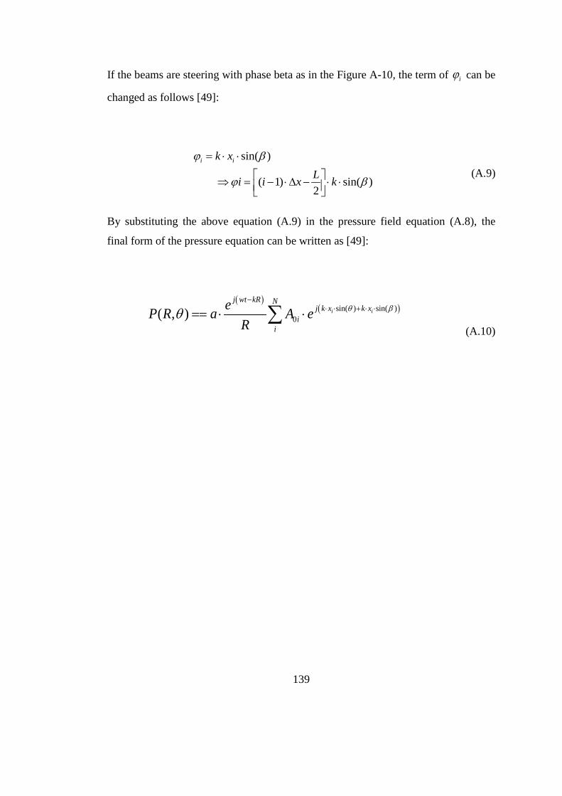
139
If the beams are steering with phase beta as in the Figure A-10, the term of iϕ can be
changed as follows [49]:
sin( )
( 1) sin( )2
i ik xLi i x k
ϕ β
ϕ β
= ⋅ ⋅
⇒ = − ⋅∆ − ⋅ ⋅
(A.9)
By substituting the above equation (A.9) in the pressure field equation (A.8), the
final form of the pressure equation can be written as [49]:
( )( )sin( ) sin( )
0( , ) i i
j wt kR Nj k x k x
ii
eP R a A eR
θ βθ−
⋅ ⋅ + ⋅ ⋅== ⋅ ⋅∑ (A.10)

140
A.2.4 Focusing with Phased Array Transducers
In the previous part, steering the ultrasonic beam was described. Ultrasonic beam can
be also formed, especially focused, with phased array transducer electronically. To
focus the beam there is no need for any focusing hardware.
Consider the array transducer in Figure A-10. Ultrasonic beam can focus at a focal
distance F along the z-axis. The corresponding phase for the element transmitting
from the origin axes is 𝜑𝜑0 = 𝑘𝑘 ∙ 𝐹𝐹. To focus at a focal point all elements should have
the same phase at the focal point. Calculation of the phase element of each element i
is as follows: multiply its distance to the focal point by the wave number and add its
initial phase 𝜑𝜑𝑖𝑖 . This expression should equal to 𝜑𝜑0 as in Equation (A.11).
2 2i ik x F k Fϕ⋅ + + = ⋅ (A.11)
After rearranging Eq. A.11, we obtain:
( )2 2ii k F x Fϕ = ⋅ − +
(A.12)
The final form of resultant pressure formulation becomes as given below:
( ) ( )2 2sin( ) sin( )
0( , ) i i ij wt kR N j k x k x k F x F
ii
eP R a A eR
θ βθ
− ⋅ ⋅ + ⋅ ⋅ + ⋅ − + == ⋅ ⋅∑
(A.13)

141
APPENDIX B
ELECTRICAL AND ACOUSTIC PROPERTIES OF
SOME HUMAN TISSUES
B.1. Electrical Properties of Some Human Tissues
Dielectric permittivity and conductivity values of some tissues are given for 50 kHz,
100 kHz, 500 kHz and 1 MHz in Table.B.1 and in Table.B.2, respectively.
Table B-1 Conductivity values of some human tissues at 50 kHz, 100 kHz, 500 kHz, and 1
MHz [38-40].
50 kHz
(S/m)
100 kHz
(S/m)
500 kHz
(S/m)
1 MHz
(S/m)
Aorta 0.3169 0.3186 0.3239 0.3267
Bladder 0.2169 0.2189 0.2279 0.2360
Blood 0.7008 0.7029 0.7482 0.8221
Bone(Cancellous) 0.0834 0.0838 0.0867 0.0903
Bone (Cortical) 0.0206 0.0207 0.0222 0.0243
Bone Marrow (Infiltrated) 0.1027 0.1028 0.1035 0.1041

142
TableB-1 Continued
Bone Marrow (Not Infiltrated) 0.0036 0.0038 0.0044 0.0047
Brain (Grey Matter) 0.1275 0.1336 0.1519 0.1632
Brain (White Matter) 0.0776 0.0818 0.0947 0.1021
Breast Fat 0.0249 0.0250 0.0254 0.0257
Cartilage 0.1771 0.1785 0.2008 0.2328
Cerebellum 0.1475 0.1536 0.1725 0.1854
Cerebro Spinal Fluid 2.0000 2.0000 2.0000 2.0000
Cervix 0.5443 0.5476 0.5569 0.5624
Colon 0.2444 0.2477 0.2778 0.3141
Cornea 0.4814 0.4993 0.5773 0.6559
Dura 0.5017 0.5018 0.5026 0.5033
Eye Tissue (Sclera) 0.5147 0.5184 0.5615 0.6188
Fat (Average Infiltrated) 0.0433 0.0434 0.0438 0.0440
Fat (Not Infiltrate) 0.0242 0.0244 0.0248 0.0250
Gall Bladder 0.9001 0.9001 0.9002 0.9002
Gall Bladder Bile 1.4000 1.4000 1.4000 1.4000
Heart 0.1954 0.2151 0.2807 0.3275
Kidney 0.1594 0.1713 0.2283 0.2782
Lens Cortex 0.3385 0.3401 0.3528 0.3745

143
Table B-1 Continued
Lens Nucleus 0.2006 0.2007 0.2013 0.2018
Liver 0.0720 0.0845 0.1481 0.1866
Lung (Deflated) 0.2620 0.2716 0.3070 0.3343
Lung (Inflated) 0.1027 0.1073 0.1230 0.1360
Muscle 0.3518 0.3618 0.4459 0.5026
Nerve 0.0693 0.0807 0.1109 0.1302
Ovary 0.3362 0.3393 0.3502 0.3579
Skin (Dry) 0.0001 0.00025 0.0042 0.0130
Skin (Wet) 0.0290 0.0654 0.1776 0.2210
Small Intestine 0.5803 0.5942 0.7147 0.8648
Spleen 0.1179 0.1221 0.1471 0.1823
Stomach 0.5337 0.5360 0.5540 0.5837
Tendon 0.3878 0.3885 0.3908 0.3920
Testis 0.4344 0.4386 0.4911 0.5620
Thyroid 0.5339 0.5369 0.5658 0.6026
Tongue 0.2842 0.2879 0.3310 0.3882
Trachea 0.3299 0.3380 0.3591 0.3732
Uterus 0.5258 0.5314 0.5495 0.5642
Vitreous Humor 1.5000 1.5000 1.5003 1.5007

144
Table B-2 Dielectric permittivity values of some human tissues at 50 kHz, 100 kHz, 500 kHz,
and 1 MHz [38-40].
50 kHz
(x1e3)
100 kHz
(x1e3)
500 kHz
(x1e3)
1 MHz
(x1e3)
Aorta 1.633 0.9299 0.3123 0.2181
Bladder 1.9123 1.2310 0.5345 0.3427
Blood 5.1976 5.1200 4.1885 3.0263
Bone(Cancellous) 0.6131 0.4717 0.30816 0.2489
Bone (Cortical) 0.2641 0.2276 0.1745 0.1445
Bone Marrow
(Infiltrated)
0.2444 0.1731 0.1095 0.0990
Bone Marrow (Not
Infiltrated)
0.1805 0.1107 0.0489 0.0397
Brain (Grey Matter) 5.4613 3.2217 1.1869 860.4221
Brain (White
Matter)
3.5481 2.1076 0.7122 0.4797
Breast Fat 1.1775 0.0706 0.0307 0.0236
Cartilage 2.7620 2.5722 1.9385 1.3908
Cerebellum 5.7555 3.5152 1.4749 1.1408
Cerebro Spinal Fluid 0.1089 0.1089 0.1089 0.1089
Cervix 3.1507 1.750 0.6140 0.4479
Colon 4.6106 3.7220 2.3702 1.6787

145
TableB-2 Continued
Cornea 16.970 10.5670 4.6365 2.8780
Dura 0.3938 0.3263 0.2644 0.2534
Eye Tissue (Sclera) 5.4946 4.7452 3.2519 2.1783
Fat (Average
Infiltrated)
0.1632 0.1014 0.0567 0.0508
Fat (Not Infiltrated) 0.1724 0.0928 0.0345 0.0272
Gall Bladder 0.1724 0.1072 0.1011 0.1002
Gall Bladder Bile 0.1199 0.1199 0.1199 0.1199
Heart 16.9823 9.8458 3.2645 1.9673
Kidney 11.4294 7.6515 3.4432 2.2514
Lens Cortex 2.6265 2.0675 1.5021 1.2267
Lens Nucleus 0.2641 0.2003 0.1476 0.1387
Liver 10.6896 7.4988 2.7698 1.5357
Lung (Deflated) 8.5314 5.1452 1.8842 1.1705
Lung (Inflated) 4.2725 2.5812 1.0249 0.7331
Muscle 10.0937 8.0891 3.6472 1.8364
Nerve 9.5874 5.1330 1.4875 0.9261
Ovary 3.010 1.9417 0.8732 678.2865
Skin (Dry) 1.1267 1.1192 1.0619 0.9907

146
TableB-2 Continued
Skin (Wet) 21.8759 15.3567 3.6100 1.8328
Small Intestine 17.4050 13.8474 8.5941 5.6755
Spleen 5.4927 4.2222 2.7889 2.2900
Stomach 3.5511 2.8609 2.0647 1.6783
Tendon 0.81497 0.4724 0.2006 0.1600
Testis 6.4863 5.7169 4.0019 2.6833
Thyroid 4.0231 3.3011 2.1395 1.4333
Tongue 5.4960 4.7456 3.2520 2.1783
Trachea 6.9124 3.7347 1.1576 0.7750
Uterus 5.6698 3.4112 1.4893 1.1675
Vitreous Humor 0.0985 0.0979 0.09134 0.0840

147
B.2.Acosutic Properties of Some Human Tissues
Table B-3. Acoustic Properties of different tissues [57]
Material Speed of Sound(m/s) Density(kg/m3) Soft tissues 1520-1580 980-1010
Lipid-based tissues 1400-1490 920-940
Collagen-based tissues 1600-1700 1020-1100
Aqueous humor 1002-1006 1500
Vitreous humor 1090 1530
Blood 1580 1040-1090
Brain-grey 1532-1550 1039
Brain-white 1532-1550 1043
Skull-compact inner and
outer tables
2600-3100 1900
Skull-spongy diploe 2200-2500 1000
Long bone-outer layer 2600-3100 1900
Long bone-inner layer 1700-2000 1100
Teeth 3500-4000 2200

148
APPENDIX C
SIGNAL-TO-NOISE RATIO OF A DATA
ACQUISITION SYSTEM
The signal-to-noise ratio (SNR) of a data acquisition system with signal s and noise n
can be defined as:
2
2
( )10log
( )E s
SNRE n
= (C.1)
where E(.) represents expected value and . represents the Euclidean norm
operations. The singular value at the truncation level (r) is the smallest singular value
that satisfies the following inequality:
120 logk
SNRσσ
≤ for k=1, …r (C.2)
If r<n, then V becomes an nxr matrix, that is, the matrix V is truncated. The
remaining basis vectors characterize the resolution matrix R.

149
CURRICULUM VITAE
PERSONAL INFORMATION
Surname, Name: Zengin, Reyhan
Nationality: Turkish (TC)
Date and Place of Birth: 1 January 1979, Malatya
Marital Status: Married
E-mail: [email protected]
EDUCATION:
Degree Institution Year of Graduation
MS&PhD METU, Electrical and Electronics Engineering 2012
BS Inonu Unv, Electrical and Electronics Engineering 2001
High School Malatya Anadolu High School, Malatya 1996
WORK EXPERIENCE
Year Place Enrollment
2003-Present METU, Dept. of Electrical and Electronics Eng. Research Assistant
FOREIGN LANGUAGES
English

150
PUBLICATIONS:
1. Zengin R., Gençer N. G., ‘ Forward Problem Solution for Electrical
Conductivity Imaging via ANSYS’, 13th Biomedical Engineering
Meeting, 2008, Ankara, Turkey
2. Zengin R., Gençer N. G., ‘Forward Problem Solution for Contactless
Electrical Conductivity Imaging with Realistic Head Model’, 14th
Biomedical Engineering Meeting 2009, İzmir, Turkey
3. Zengin R., Gençer N. G., ‘Sensitivity Matrix Analysis for Contactless
Electical Conductivity Imaging, 15th Biomedical Engineering Meeting
2010 , Antalya, Turkey
4. Zengin R., Gençer N. G., ‘Dokunmasız Elektrik İletkenlik Görüntülemesi
için Gerçekçi Kafa Modeli ile Duyarlılık Matrisi Analizi,’ V. URSI-
TURKIYE’2010, METU-Northern Cyprus Campus, North Cyprus
Turkish Republic


![electrical impedance tomography - Aaltolib.tkk.fi/Diss/2008/isbn9789512296804/article1.pdf · [I] Two-stage reconstruction of a circular anomaly in electrical impedance tomography](https://static.fdocuments.us/doc/165x107/5b7a88557f8b9a22238c5728/electrical-impedance-tomography-i-two-stage-reconstruction-of-a-circular.jpg)