Clemson UniversityTigerPrints

All Theses Theses

12-2018

Comparison of Electrical Impedance TomographyReconstruction Algorithms With EIDORSReconstruction SoftwareMatthew BrinckerhoffClemson University, mattbrinckerhoff@gmail.com

Follow this and additional works at: https://tigerprints.clemson.edu/all_theses

This Thesis is brought to you for free and open access by the Theses at TigerPrints. It has been accepted for inclusion in All Theses by an authorizedadministrator of TigerPrints. For more information, please contact kokeefe@clemson.edu.

Recommended CitationBrinckerhoff, Matthew, "Comparison of Electrical Impedance Tomography Reconstruction Algorithms With EIDORSReconstruction Software" (2018). All Theses. 2973.https://tigerprints.clemson.edu/all_theses/2973

Comparison of Electrical ImpedanceTomography Reconstruction Algorithms With

EIDORS Reconstruction Software

A ThesisPresented to

the Graduate School of Clemson University

In Partial Fulfillmentof the Requirements for the Degree

Master of ScienceMathematics

byMatthew Brinckerhoff

December 2018

Accepted by:Dr. Taufiquar Khan, Committee Chair

Dr. Shitao LiuDr. Jeong Yoon

Abstract

Electrical impedance tomography (“EIT”) has many significant applications,

ranging from geophysical and medical imaging, to the military, to industrial fields.

Due to the relevance of EIT in fields of critical importance to society, further de-

velopment of EIT is vital. The instability of image reconstruction and the highly

nonlinear behavior of the image reconstruction problem, make the problem particu-

larly difficult, are referred to as ill-posed inverse problem. Specifically, development

of a comprehensive set of techniques to solve the EIT problem is necessary, due to

both its ill-posed, nonlinear nature, and its scope. In this thesis, several approaches

to the inversion of the EIT problem are presented, as well as a comparison with the

inversion software EIDORS (Electrical Impedance Tomography and Diffuse Optical

Tomography Reconstruction Software).

In this thesis, the advantages and disadvantages of EIT as compared to other

imaging techniques is discussed. Then the theory of EIT, including the governing

equations, the forward problem, and methods for solving the inverse problem are

presented. Next, the reconstruction software EIDORS is presented, in which artificial

data is created, and the reconstruction algorithms are implemented. The effect of

noise on the simulated data is investigated. Lastly, experimental data is implemented,

and the results are discussed. We considered absolute conductivities in reconstruction,

which was a gap in previous work, and have thus resolved this missing element of the

ii

work.

The experimental data was successfully reconstructed with two different ab-

solute reconstruction algorithms. Additionally, the optimal injection patterns were

evaluated for accuracy and practical application. Lastly, we observed that the re-

construction algorithms were extremely sensitive to the regularization parameter,

implying that the parameter selection method is of paramount importance.

In this thesis, we have considered smoothness constraints such as TV regu-

larization and L2 regularization which leads to reasonable reconstruction using ex-

perimental data and leads the way for future comparison to sparsity and statistical

approaches to solve the EIT inverse problem.

iii

Acknowledgments

I am grateful for the faculty and staff of the Clemson Department of math-

ematical sciences for preparing me to perform this research. I also am grateful for

Dr. Farrel Martin of the Naval Research Laboratory for introducing me to the re-

construction software EIDORS. I would like to give a special ”Thank you” to Dr.

Taufiquar Khan for his support, guidance, mentorship, and enthusiasm. I also would

like to thank Dr. Jeong-Rock Yoon and Dr. Shitao Liu for serving on my thesis

committee. I also thank Dr. Tao Ruan and Dr. Amir Poursaee for providing the

experimental data. Lastly, I thank my peers Sanwar Ahmad, Scott Scruggs, Shyla

Kupis, and Thowhida Akther for their support and time both in class and in preparing

this research.

iv

Table of Contents

Title Page . . . . . . . . . . . . . . . . . . . . . . . . . . . . . . . . . . . i

Abstract . . . . . . . . . . . . . . . . . . . . . . . . . . . . . . . . . . . . ii

Acknowledgments . . . . . . . . . . . . . . . . . . . . . . . . . . . . . . . iv

List of Tables . . . . . . . . . . . . . . . . . . . . . . . . . . . . . . . . . vi

List of Figures . . . . . . . . . . . . . . . . . . . . . . . . . . . . . . . . . vii

1 Introduction . . . . . . . . . . . . . . . . . . . . . . . . . . . . . . . . 31.1 Background . . . . . . . . . . . . . . . . . . . . . . . . . . . . . . . . 31.2 Objectives . . . . . . . . . . . . . . . . . . . . . . . . . . . . . . . . . 5

2 EIT Theory: Forward and Inverse Problem . . . . . . . . . . . . . 72.1 Governing Equations for the Forward Model . . . . . . . . . . . . . . 82.2 Gauss-Newton Method for the Inverse Problem . . . . . . . . . . . . 102.3 Method of Total Variation for the Inverse Problem . . . . . . . . . . . 142.4 Hyperparameter Selection . . . . . . . . . . . . . . . . . . . . . . . . 172.5 EIDORS . . . . . . . . . . . . . . . . . . . . . . . . . . . . . . . . . . 20

3 Experimentation . . . . . . . . . . . . . . . . . . . . . . . . . . . . . . 22

4 Results . . . . . . . . . . . . . . . . . . . . . . . . . . . . . . . . . . . 254.1 Simulated Data . . . . . . . . . . . . . . . . . . . . . . . . . . . . . . 254.2 Experimental Data . . . . . . . . . . . . . . . . . . . . . . . . . . . . 39

5 Conclusions and Discussion . . . . . . . . . . . . . . . . . . . . . . . 435.1 Future Work . . . . . . . . . . . . . . . . . . . . . . . . . . . . . . . . 45

Appendices . . . . . . . . . . . . . . . . . . . . . . . . . . . . . . . . . . . 46A A Starting Guide to EIDORS . . . . . . . . . . . . . . . . . . . . . . 47

Bibliography . . . . . . . . . . . . . . . . . . . . . . . . . . . . . . . . . . 50

v

List of Tables

4.1 Average values of the 1-norm and 2-norm from 10 samples using equa-tion 4.1 corresponding to figures 4.2 and 4.3 for noise levels of 1, 3,5, 10, and 15 percent using the Gauss-Newton Method and Method ofTotal Variation . . . . . . . . . . . . . . . . . . . . . . . . . . . . . . 27

4.2 Values of the 1-norm and 2-norm using equation 4.1 corresponding tofigure 4.4, for various hyperparameter values in the adjacent currentinjection pattern . . . . . . . . . . . . . . . . . . . . . . . . . . . . . 31

4.3 Values of the 1-norm and 2-norm using equation 4.1 corresponding tofigure 4.5, for various hyperparameter values in the opposite currentinjection pattern . . . . . . . . . . . . . . . . . . . . . . . . . . . . . 31

4.4 Values of the 1-norm and 2-norm using equation 4.1 corresponding tofigure 4.6, for various hyperparameter values in the sinusoidal currentinjection pattern . . . . . . . . . . . . . . . . . . . . . . . . . . . . . 31

4.5 Values of the 1-norm and 2-norm using equation 4.1 corresponding tofigure 4.8, for various hyperparameter values using the Gauss-NewtonMethod . . . . . . . . . . . . . . . . . . . . . . . . . . . . . . . . . . 34

4.6 Values of the 1-norm and 2-norm using equation 4.1 corresponding tofigure 4.9, for various hyperparameter values using the Total VariationMethod . . . . . . . . . . . . . . . . . . . . . . . . . . . . . . . . . . 37

4.7 Values of the 1-norm and 2-norm using equation 4.1 corresponding tofigure 4.13, for various hyperparameter values using the Gauss-Newtonmethod . . . . . . . . . . . . . . . . . . . . . . . . . . . . . . . . . . 41

4.8 Values of the 1-norm and 2-norm using equation 4.1 correspondingto figure 4.14, for various hyperparameter values using the method oftotal variation . . . . . . . . . . . . . . . . . . . . . . . . . . . . . . . 41

vi

List of Figures

2.1 Simulated Region (Left) and Reconstruction using the Gauss-NewtonMethod with a hyperparamter value of zero (Right). . . . . . . . . . . 18

2.2 FEM mesh from Netgen, with electrodes shown in green. Observe thelarger elements in the center and smaller elements near the electrodes. 21

3.1 Image of experimental specimen with conductive paint and a singleinclusion [12] . . . . . . . . . . . . . . . . . . . . . . . . . . . . . . . 23

3.2 Depiction of the first current injection and measurement patterns forthe experiment [12] . . . . . . . . . . . . . . . . . . . . . . . . . . . . 24

4.1 Geometry of the forward model. Inclusion shown in blue, electrodes ingreen. . . . . . . . . . . . . . . . . . . . . . . . . . . . . . . . . . . . 26

4.2 Reconstruction of simulated data from figure 4.1 with noise levels of1,3,5,10,and 15 percent, using the Gauss-Newton Method . . . . . . . 28

4.3 Reconstruction of simulated data from figure 4.1 with noise levels of1,3,5,10,and 15 percent, using the Method of Total Variation . . . . . 29

4.4 Reconstruction of figure 4.1 using an adjacent injection pattern, forhyperparameter values of .002, .003, .004, .005, .006 . . . . . . . . . . 30

4.5 Reconstruction of figure 4.1 using opposite current injection pattern,for hyperparameter values of .002, .003, .004, .005, .006 . . . . . . . . 32

4.6 Reconstruction of figure 4.1 using sinusoidal current injection pattern,for hyperparameter values of .002, .003, .004, .005, .006 . . . . . . . . 33

4.7 Geometry of the forward model with two distinct inclusions. . . . . . 344.8 Reconstruction of figure 4.7 with the Gauss-Newton method, for hy-

perparameter values of .002, .003, .004, .005, .006 . . . . . . . . . . . 354.9 Reconstruction of figure 4.7 with the Total Variation method, for hy-

perparameter values of .002, .003, .004, .005,.006 . . . . . . . . . . . . 364.10 Reconstruction of figure 4.7 with the method of total variation and

hyperparameter value of .001 . . . . . . . . . . . . . . . . . . . . . . . 374.11 Top: Simulated models with centered inclusions of radius 100mm,

70mm, and 50mm, Bottom: Reconstruction of these models with theGauss-Newton Method . . . . . . . . . . . . . . . . . . . . . . . . . . 38

4.12 Recreation of figure 3.1 in EIDORS . . . . . . . . . . . . . . . . . . . 39

vii

4.13 Reconstruction of Experimental data using the Gauss-Newton method,for hyperparameter values of .0009, .001, .0011, .0012, .0013 . . . . . 40

4.14 Reconstruction of Experimental data using the method of total varia-tion, for hyperparameter values of .14, .15, .16, .17, .18 . . . . . . . . 41

1 Sample EIDORS Code . . . . . . . . . . . . . . . . . . . . . . . . . . 49

viii

List of Symbols

∇· Divergence Operator

∇ Gradient operator

Ω Domain of the Region

σ Conductivity Vector

u Electric Potential

x A cartesian location in the domain

∂Ω Boundary of the domain

∂ Partial Derivative

El Surface area of the Lth electrode

Il Current injected into the lth electrode

n outward unit normal vector

dS Surface element of the domain

Ul Electric Potential on the lth electrode

zl Contact Impedance

F Forward operator that maps σ to Ul

1

Ul,meas Vector of measured potentials at the electrodes

λ Regularization/Hyperparameter

ε Noise in the measured data

σ0 Background conductivity

δσ Change in conductivity from one iteration to the next

J Jacobian Matrix

2

Chapter 1

Introduction

1.1 Background

Electrical impedance tomography (EIT) is a nondestructive and harmless tech-

nique for estimating conductivity of an unknown or inaccessible region [5]. EIT is

used in situations where the conductivity of an area of interest cannot be measured

directly. Instead, measurements are taken at the boundary of the domain, and the

conductivity of the region is estimated using the technique of mathematical inversion.

In all but the simplest of cases, this inversion is an ill-posed problem–one with more

unknown parameters than known measurements. An ill-posed problem, as defined

by Hadamard, fails to adhere to one of the following three properties: (1) A solution

exists, (2) The solution is unique, and (3) small changes in the data results in small

changes in the solution [10].

This leads to the possibility of multiple simultaneous solutions to the conduc-

tivity distribution, when in reality there is only one true conductivity distribution.

To resolve the ill-posed nature of the inverse problem, regularization techniques are

introduced which use prior information to force solutions to converge, hopefully to

3

the true, real life values.

In practical applications, the validity of the inverse solution is not certain. But

we can perform experiments on domains for which we know the true conductivity,

and compare the inversion results to the known values. In this way, we can at least

generate some confidence for the inversion methods that are used.

EIT can be applied in a wide range of fields. EIDORS software is focused on

geophysical and medical applications, but really can be used in any situation where the

conductivity of a non-measurable region is desired. Some other applications include

electrochemical cells and corrosion of conductive materials.

EIT is especially useful in the medical field, because it is noninvasive and

harmless, as compared to MRI and CT scans, which are both expensive and time

consuming. EIT provides lower resolution than MRI and CT scans, but EIT provides

information about the physical properties of the body [5].

The other major use of EIT is geophysical imaging [11]. EIT can be used to

monitor water reservoirs, map areas of interest for construction, and assess well-bore

integrity. Monitoring of water reservoirs is crucial as disruptions in water quality,

be it due to contamination, loss of water, or decreased access to water, can have

significant detrimental impacts on local communities. EIT can be used to survey

areas for construction, ensuring the integrity of the earth upon which structures will

be built, and ultimately the safety of the structure. Well-bore integrity is becoming

a more critical problem as the number of uses for carbon dioxide injection increases,

including the use of CO2 injection to reduce greenhouse gas emissions [6]. Geophysical

monitoring allows for observation of the changes to the physical parameters of the

aquifer or injection well. Changes can be signs of disruptions to the aquifer that

signal contamination, or leaks in the CO2 injection wells. Without monitoring, these

changes can go unnoticed, causing detrimental impacts to the water system, or in the

4

case of CO2 injection, to the environment.

Advances in the field of EIT are crucial to the health and safety of society,

and are especially important due to the use of EIT in a wide range of applications.

EIDORS is comprehensive EIT reconstruction software that can be used in all the

applications listed above, so its development and improvement also is crucial. Com-

parison of EIDORS to other EIT reconstruction algorithms is important to verify

usefulness and accuracy.

1.2 Objectives

The main objective of this thesis is to compare EIT reconstruction methods

using EIDORS. Specifically, EIDORS was used to:

1. Fill a gap in the work in the Clemson civil engineering department [12] by

reconstructing absolute conductivities and evaluating the accuracy of the images

for various reconstruction methods.

2. Investigate the effect of noise on simulated data reconstructions.

3. Compare and evaluate different injection patterns.

4. Observe the effects of changing the regularization parameter (hyperparameter).

5. Compare two different reconstruction algorithms: The Gauss-Newton Method

and the Method of Total Variation.

6. Reconstruct experimental EIT data.

The goal of this thesis is to provide a variety of methods and guidance as to

which method is optimal. It is paramount to note that the optimal method varies

5

widely for different geometries, conductivity distributions, and experimental setups.

This thesis aims to guide researchers in determining the best method for their exper-

iments.

6

Chapter 2

EIT Theory: Forward and Inverse

Problem

Electrical impedance tomography experiments implement electrodes spread

across the boundary of the area of interest. In geophysical applications, the electrodes

are placed on the surface of the earth, whereas in medical application they are placed

around the body. These electrodes are use both to induce a current within the domain,

and to measure voltages at the boundary.

In most EIT experiments, multiple injection patterns are performed, and for

each pattern multiple voltage measurements are made. Typically, in an experiment

of L electrodes, L injection patterns will be performed, each with L measurements.

This gives a total of LxL measurements to be used for mathematical inversion.

Cheney [3] discusses the optimal injection patterns for different types of con-

ductivity distributions. The most common injection patterns are adjacent, opposite,

and sinusoidal. In the adjacent pattern, electrode j is given a positive current, and

electrode j+1 is given a positive current of the same magnitude. This is repeated

for each electrode, j ∈ 1, , L. In the opposite injection pattern, electrode j is given

7

a positive current and electrode L/2+j is given a negative current. In the sinusoidal

injection pattern, a current is injected at each electrode, with a value of sin(θ), with

θ being the angle of the electrode position around the unit circle in radians. The

most common measurement pattern is the measure of the voltage across adjacent

electrodes. Thus electrode j will be included in the measurement from j-1 to j, and

from j to j+l.

Cheney [3] derives the optimal injection pattern for various geometries. It

was found that the best current pattern for a central inclusion is the sinusoidal pat-

tern. But this pattern is much more difficult to implement experimentally, because it

requires a different current for each electrode, meaning much more hardware and in-

creased costs. The opposite and adjacent patterns only require two different currents

of opposite sign, which is much less expensive to implement. For a centered inclusion,

Cheney [3] shows that the opposite current injection gives more distinguishability

than the adjacent. Distinguishability is defined as the ability to distinguish between

regions of different conductivities. The advantage of the opposite pattern is due to

the fact that the opposite pattern detects more information about the center of the

domain, whereas the adjacent pattern detects more information at the boundary.

2.1 Governing Equations for the Forward Model

The forward EIT problem is derived from Maxwell’s equations as described by

Cheney [5], and gives equation 2.1.

∇ · σ(x)∇u(x) = 0, x ∈ Ω (2.1)

Here, ∇· represents the divergence, and ∇ the gradient.Ω ∈ Rn is the domain–

8

the region of interest. Both the conductivity, σ, and electric potential, u, are vectors

dependent on the location x in the domain.

Since EIT is mainly used in inverse problems where information is taken from

the boundary, we assume that current is injected only at the electrodes on the bound-

ary of the domain, denoted ∂Ω. This assumption leads us to equations 2.2 and 2.3.

∫El

σ∂u(x)

∂ndS = Il l = 1, 2, ..., L (2.2)

σ∂u(x)

∂n= 0 on ∂Ω/

L⋃l=1

El (2.3)

Equation 2.2 says the integral of current density on an electrode is equal to

the current flowing through that electrode. El is the surface area of the lth electrode,

Il is the current injected into El, and L is the total number of electrodes. n is the

outward unit normal vector, and dS is the surface element.

Equation 2.3 denotes that there is no current flowing in the gaps between

electrodes.

If we let Ul be the electric potential on electrode l, then we have,

u = Ul on El l = 1, 2, ..., L. (2.4)

But, equation 2.4 fails to account for what is called the double layer impedance,

or contact impedance. Contact impedance can be thought of as a thin, highly resistive

region between the electrode and the surface of the specimen. The size of this region

is at the molecular level, and can be attributed to the transfer of electrons from one

material to another. In electrochemical scenarios, the term double layer refers to

the region between an electrode and the ions in the electrolyte, where a capacitance

9

prevents the transfer of electrons from ions to the electrode. A similar concept applies

to medical EIT, where the transfer of electrons from an electrode into the body is

hindered by contact impedance [7].

The effect of contact impedance introduces a new term into the complete

electrode model, zl, the effective contact impedance. Thus 2.4 becomes

u+ zlσ∂u(x)

∂n= Ul on El l = 1, 2, ..., L. (2.5)

Lastly, we have the conservation of charge (2.6) and a specified ground level

for potential (2.7).

L∑l=1

Il = 0 (2.6)

L∑l=1

Ul = 0 (2.7)

Equation 2.6 applies due to the design of EIT experiments where every induced

current is matched by a current of the same magnitude and opposite sign.

Thus the complete electrode model consists of equations 2.1, 2.2, 2.3, 2.5, 2.6,

and 2.7.

This is the model used by EIDORS to create simulated data, and has been

shown by Somersalo [14] to predict experimental measurements to better than .1%.

2.2 Gauss-Newton Method for the Inverse Prob-

lem

The Gauss-Netwon Method is a linear approximation to the nonlinear inverse

problem, as described by Cheney [4] and Ruan [12]. The goal of this approach is to

10

minimize the objective function J(σ) in equation 2.8.

J(σ) = ||Ul,meas − F (σ)||22 (2.8)

where Ul,meas is the vector of measured electric potentials on the electrodes and F

is an operator that maps the vector of conductivity estimates to the corresponding

voltage measurements through the solution of the forward problem. If we let ε be the

noise of the measured data, then the true potentials and measured potentials differ

by the vector ε (equation 2.9).

Ul = Ul,meas + ε (2.9)

Due to the ill-posed nature of the inverse problem as discussed above, we

introduce a regularization term so that the algorithm will converge. In particular,

we introduce Tikhonov regularization, which introduces prior information into the

minimization functional [8]. In EIT, it is common to use a constant background

conductivity as the prior information. Call this background σ0, and our minimization

functional becomes:

Jλ(σ) = ||Ul,meas − F (σ)||22 + λ||σ − σ0||22, (2.10)

where λ is commonly referred to as the hyperparameter, and will be discussed in

section 2.3.

We now summarize the steps of the Gauss-Newton Method for EIT:

1. Obtain experimental or simulated data.

2. Obtain an initial guess for the conductivity, σ0. This can be based on prior

information, or direct measurement.

11

3. Obtain the hyperparameter value.

4. Solve the forward problem to obtain F (σk)

5. Evaluate the stopping rule: either a fixed number of iterations, an accuracy

threshold, or both.

6. Calculate ∆σ, which requires the Jacobian Matrix.

7. Update the conductivity

σk+1 = σk + ∆σ (2.11)

8. Update the admittance matrix used to solve the forward problem.

9. Update the Jacobian Matrix.

10. Return to step 4.

The key step here is the calculation of ∆σ, which is determined throught the

calculation of the Jacobian Matrix, as discussed below.

2.2.1 Calculation of the Jacobian Matrix

The derivation of the Jacobian Matrix, also called the sensitivity matrix, is

presented by Graham [8] and Ruan [12]. The goal is to find a matrix, J, that satisfies

the equation

Ul,meas − Uc = J∆σ (2.12)

where Uc = F (σk), the vector of potentials, is calculated by solving the forward

problem given σk. The Jacobian Matrix is also called the sensitivity matrix because

it describes how changes in the conductivity affect the change in potentials.

First, we observe the weak form of equation 2.1, for a test function ν.

12

∫Ω∇ · (σ∇u)νdx = 0 (2.13)

Applying integration by parts we arrive at

∫∂Ω

⋂El

σ∂u

∂nνdS +

∫∂Ω/El

σ∂u

∂nνdS −

∫Ωσ∇u · νdV = 0 (2.14)

By equation 2.3, the second term is zero, and dV denotes a volume element.

∫∂Ω

⋂El

σ∂u

∂nνdS =

∫Ωσ∇u · ∇νdV (2.15)

Substituting u for ν, and equation 2.5 for the left hand side gives

∫∂Ω

⋂El

σ∂u

∂n(Ul − zlσ

∂u

∂n)dS =

∫Ωσ|∇u|2dV (2.16)

Now, summing over each electrode El, and applying equation 2.2 we arrive at,

L∑l=1

UlIl =∫

Ωσ|∇u|2dV +

L∑l=1

∫El

zl(σ∂u

∂n)2dS (2.17)

Next, we take perturbations δσ, δu, δUl to first order, along with equation 2.5,

and the weak formulation with ν = δu.

L∑l=1

δUlIl =∫

Ωδσ|∇u|2dV + 2

L∑l=1

∫El

δUlσ∂u

∂ndS (2.18)

Substituting equation 2.2 into the final term and subtracting that term we

have

−L∑l=1

δUlIl =∫

Ωδσ|∇u|2dV (2.19)

13

For a single injection pattern i, and a single measurement m, equation 2.19

becomes [12] :

δUi,m = −∫

Ωδσ∇ui · ∇umdV (2.20)

Next, consider the finite elements in the discretization of the domain, Ω, and

assume conductivity to be constant over individual elements. Let δσ be this discretiza-

tion, and we arrive finally at the equation for the Jacobain of the mth measurement

in the ith injection pattern [12] :

J =∂Uim∂σ

= −∫

Ω∇ui · ∇umdV (2.21)

On each step, ∆σ is the minimization of

||(Ul,meas − F (σ))− J∆σ||22 + λ||σ − σ0||22 (2.22)

over all ∆σ, which has the solution:[8]

∆σ = (JTJ + λ2I)−1JT (Ul,meas − F (σ)), (2.23)

where I is the identity matrix.

2.3 Method of Total Variation for the Inverse Prob-

lem

The method of total variation is a nonlinear method for solving the inverse

problem. It is described by Graham [8] and Ruan [12], and requires the Jacobian

Matrix described above. The advantage of this method is that it allows for disconti-

14

nuities in the reconstruction image [8]. This means sharp changes in conductivities

can be accurately detected. This attribute of the total variation method is useful

for medical and geophysical applications, and for other scenarios involving discontin-

uous domains. The difficulty of this method is that it involves computation of the

minimum of a non-differentiable function, which increases computational costs and

time.

The goal of this method is to minimize

Jλ(σ) = ||Ul,meas − F (σ)||2 + λTV (σ) (2.24)

where

TV (σ) =∫

Ω|∇σ|dΩ (2.25)

If we assume the conductivity is constant of each element of the finite element

mesh, and let k be the number of edges in the mesh, then equation 2.25 becomes

TV (σ) =∑k

lk|σ(1)k − σ

(2)k | =

∑k

|Lkσ| = Lσ. (2.26)

where lk is the length of the kth edge, and |σ(1)k − σ

(2)k | is the difference in the

conductivities on either side of edge k. Considering the matrix form of Lk of lk, and

vector form σ of σ we arrive at

TV (σ) =∑k

|Lkσ|. (2.27)

To find the minimum of equation 2.24 we implement the Primal Dual-Interior

Point Methods(PD-IPM), which is described in detail by Borsic [2]. First, observe

15

the dual problem to the minimization of equation 2.24, which is to find the maximum

of

||Ul,meas − F (σ)||2 + λyTLσ. (2.28)

where y ∈ is such that ||yi|| < 1 [8]. Subtracting equation 2.28 from equation 2.24

leads to

∑k

|Lkσ| − yTLσ| = 0 (2.29)

The system of equations defining the PD-IPM method [8] are as follows:

JT (Ul,meas − F (σ)) + λLσ = 0 (2.30)

Lσ − Ey = 0. (2.31)

wher J is the Jacobian Matrix and E is a diagonal matrix that contains an extra

parameter, β. beta is called the smoothness parameter, and it ensures that the non-

differentiable problem does not diverge.

E = diag(√||Liσ||2 + β i = 1, 2, .., n (2.32)

Newton’s method can be used to solve the PD-IPM method (equations 2.30

and 2.31), which gives the conductivity update as

∆σj = (JTj Jj + λLTE−1j KL)−1(JTj (∆Uj − F (σj) + λLTE−1

j Lσj) (2.33)

16

where

∆Uj = Ul,meas − F (σj) (2.34)

is also the stopping criteria, and

K = diag(1− yiLiσ

E(i, i)). (2.35)

The initial guess sets y = 0 and E = I, the identity matrix. On each step, the

Jacobain J , ∆U , E and y must be updated. The update to y is given by

∆yj = yj + E−1j Lσj + E−1

j KjL∆σj (2.36)

This process continues until a certain number of iterations is reached, or equa-

tion 2.34 becomes small enough to satisfy the stop criteria. It is clear that the method

of total variation is much more computationally expensive, but it also better identifies

sharp conductivity changes.

2.4 Hyperparameter Selection

The hyperparameter, λ, in equations 2.10 and 2.23, controls the amount of

regularization in the image reconstruction. As λ increases, more weight is put on the

regularization term, which for Tikhonov regularization means the solution is pushed

towards the prior distribution. If λ = 0, then no regularization is applied, and the

ill-posed problem can become very unstable. Figure 2.1 shows the instability when

λ = 0 is chosen.

The goal of the selection of a hyperparameter is to simply produce a more

accurate reconstruction of the conductivity distribution. One may think this implies

17

Figure 2.1: Simulated Region (Left) and Reconstruction using the Gauss-NewtonMethod with a hyperparamter value of zero (Right).

the prior information should be given as little weight as possible, but this is not the

case due to the ill-posed nature of the problem. In this section, we discuss three of

the most widely used hyperparameter selection methods: Heuristic, L-Curve, and the

Fixed Noise Figure as presented in [9].

Heuristic hyperparameter selction is the most widely used method in EIT, even

though it is the most subjective. In this method, a wide range of hyperparameter

values are used in reconstruction. Then, the researcher chooses the image that looks

best.“Best” here being a subjective choice. In general, the best image usually means

the image with the most resolution and least noise. An experiment by Graham

(source) concluded that heuristic hyperparameter selection is neither consistent nor

repeatable.

In the L-Curve method, the semi-norm of the regularized solution, ln||∆σ||, is

plotted against the norm of the residual vector, ln||J(∆σ)−(Ul,meas−Uc)||, for a range

of λ values. The optimal λ value is selected to be the point of maximum curvature.

18

This method is called L-Curve because the curve is typically L-shaped, and the best

value is the corner of the “L”. The L-Curve method is the most unbiased, but it can

sometimes be difficult to identify a corner in the curve.

The Fixed Noise Figure (NF) method uses the ratio of the signal-to-noise ratio

of the measurements to the signal-to-noise ratio of the reconstructed conductivity.

This ratio, denoted NF, is defined by

NF =SNRm

SNRr

. (2.37)

The NF method is also heuristic because instead of choosing λ, the researcher

chooses a value for NF. Experimental results have shown that NF values between .5

and 2 give good reconstructions [9]. Once the NF value is selected, the hyperparam-

eter value is found using a bisection search technique. The NF method is the most

reliable in that it always selects a hyperparameter with a good reconstruction image.

All three of these methods are widely used in EIT. The L-Curve method does

not always work, as the curve is not always L-shaped. The NF method is suitable

for any configuration, but still employs heuristic selection of the NF value. Heuristic

hyperparameter selection allows the researcher to choose the noise and resolution level

that best suits the experiment, but it is the most biased. Graham [9] describes a new

method that is a combination of the others, called “BestRes.” This method still does

not guarantee a selection of the optimal hyperparameter value, but it does perform

well as an objective approach. Future work is necessary to determine or generate the

optimal method for the selection of the hyperparameter.

19

2.5 EIDORS

EIDORS, along with Netgen meshing software, was used to simulate artificial

data and reconstruct this data and experimental data with a variety of methods

and algorithms. Some EIDORS functions are described in [1], but the majority

of functions and the inner workings of EIDORS is not provided. For this reason,

Appendix A has been included in this thesis to facilitate the use of EIDORS in the

future. Netgen [13] is a software called by EIDORS to make the geometry, place

electrodes, and generate the FEM mesh.

EIDORS models, which match experimental design, have a few common char-

acteristics. The number of electrodes, Ne, typically has values of Ne = 2n for

n = 1, 2, .... Most commonly, 16 or 32 electrodes are used. These electrodes are

numbered in a clockwise manner starting with the topmost electrode, as depicted in

figure 4.2. Adjustments can be made to change the electrode numbering, which is

described in Appendix A.

There are two ways to define a region of different conductivity from the back-

ground. Firstly, simply define a region using an equation (for example the equation

of a circle), and define the conductivity of all nodes within that region. Alternatively,

a second EIDORS object can be defined, which is a useful approach for more complex

geometries. Then, the conductivity of individual objects can be defined in EIDORS.

Netgen creates complex finite element meshes that are ideal for EIT inverse

problems. As seen in figure 2.2, there are more elements at the boundary and fewer

towards the center of the domain. Since data is collected at the boundary, on the

electrodes, it is beneficial to have more elements at the boundary because more in-

formation is known near the electrodes.

EIDORS can be used to simulate artificial data, as well as to solve the inverse

20

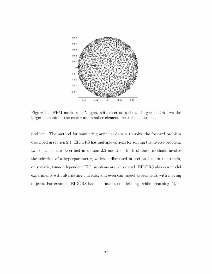
Figure 2.2: FEM mesh from Netgen, with electrodes shown in green. Observe thelarger elements in the center and smaller elements near the electrodes.

problem. The method for simulating artificial data is to solve the forward problem

described in section 2.1. EIDORS has multiple options for solving the inverse problem,

two of which are described in section 2.2 and 2.3. Both of these methods involve

the selection of a hyperparameter, which is discussed in section 2.4. In this thesis,

only static, time-independent EIT problems are considered. EIDORS also can model

experiments with alternating currents, and even can model experiments with moving

objects. For example, EIDORS has been used to model lungs while breathing [1].

21

Chapter 3

Experimentation

The data used in this thesis was obtained by Dr. Tao Ruan [12], in an effort to

identify surface damages in cement. The research presented in this thesis is designed

to compare different EIT reconstruction models; thus, comparison with real (not

simulated) data is imperative.

A cylindrical slab of concrete was prepared with a water-to-cement ratio of

.45. The dimensions of the slab were 50mm in height and 100mm in diameter. Next,

in order to produce a conductive region, the top surface of the specimen was sprayed

with a nickel-based conductive paint. A circular area was covered with masking

tape, and thus not painted, in order to represent an inclusion. This inclusion had a

diameter of 25mm and was centered midway between the center of the specimen and

the edge of the specimen. The conductive paint had a conductivity of 1.4 Siemens per

meter. The conductivity of cement is much lower, meaning the unpainted inclusion

was essentially non-conductive. An image of the specimen is shown in figure 3.1.

Next, electrodes were placed on the top surface, allowing for 2D reconstruc-

tion imaging. Sixteen equally spaced, serrated-tip electrodes were placed around the

edge of the top surface. The electrodes had a diameter of 5mm. The serrated tips

22

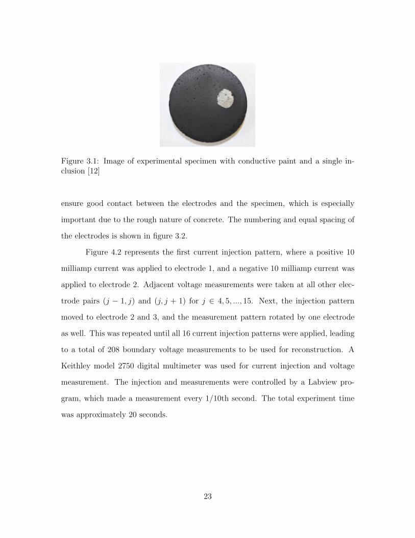
Figure 3.1: Image of experimental specimen with conductive paint and a single in-clusion [12]

ensure good contact between the electrodes and the specimen, which is especially

important due to the rough nature of concrete. The numbering and equal spacing of

the electrodes is shown in figure 3.2.

Figure 4.2 represents the first current injection pattern, where a positive 10

milliamp current was applied to electrode 1, and a negative 10 milliamp current was

applied to electrode 2. Adjacent voltage measurements were taken at all other elec-

trode pairs (j − 1, j) and (j, j + 1) for j ∈ 4, 5, ..., 15. Next, the injection pattern

moved to electrode 2 and 3, and the measurement pattern rotated by one electrode

as well. This was repeated until all 16 current injection patterns were applied, leading

to a total of 208 boundary voltage measurements to be used for reconstruction. A

Keithley model 2750 digital multimeter was used for current injection and voltage

measurement. The injection and measurements were controlled by a Labview pro-

gram, which made a measurement every 1/10th second. The total experiment time

was approximately 20 seconds.

23

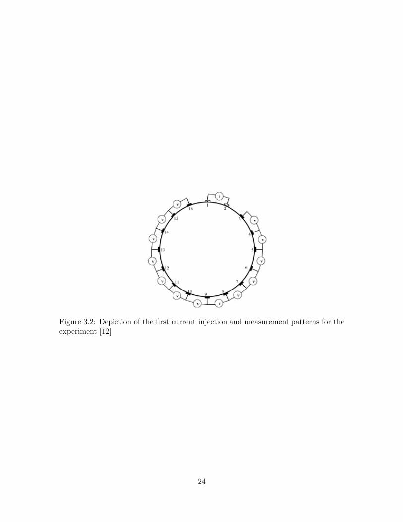
Figure 3.2: Depiction of the first current injection and measurement patterns for theexperiment [12]

24

Chapter 4

Results

4.1 Simulated Data

EIDORS functions allow for quick simulation of artificial data. The details of

these functions and their uses are described in Appendix A. The basic steps are as

follows.

1. The geometry of the object domain is created. In this case the geometry is a

simple 2D circle of radius 50mm.

2. The electrode positions, sizes, and injection and measurement patterns are de-

fined. In this case, there are 16 electrodes, an adjacent measurement pattern,

and various injection patterns (as specified in the next sections).

3. The conductivity of the geometry is specified, including any areas with different

conductivity from the background.

4. The artificial measured voltages are obtained through solving of the forward

model, which is described in the previous section 2.1.

25

Figure 4.1: Geometry of the forward model. Inclusion shown in blue, electrodes ingreen.

The geometry used to generate the artificial data is a circle with radius 500mm,

with a single inclusion centered at (242mm,150mm) with radius 100mm. The EI-

DORS geometry is shown in figure 4.1.

Once the artificial data is obtained, the inverse problem can be solved in the

same way as with real data, reconstructing the image in order to estimate the true

conductivity’s of the domain.

4.1.1 Impact of Noise on Simulated Data

We simulated data in EIDORS (Figure 4.1), and added 1, 3, 5, 10, and 15

percent noise before solving the inverse problem. The reconstruction images are

shown in figures 4.2 and 4.3. Ten different samples of the noise were simulated

and reconstructed for each noise level, and the average accuracy of all samples was

26

Noise Level (percent) 1 3 5 10 151-norm Gauss-Newton .0298 .0419 .0562 .1032 .15142-norm Gauss-Newton .0622 .0695 .0810 .1210 .16821-norm Total Variation .0490 .0591 .0710 .1057 .14522-norm Total Variation .0893 .0943 .1048 .1487 .2046

Change in data do to noise (percent) .0084 .0236 .0384 .0791 .1148

Table 4.1: Average values of the 1-norm and 2-norm from 10 samples using equation4.1 corresponding to figures 4.2 and 4.3 for noise levels of 1, 3, 5, 10, and 15 percentusing the Gauss-Newton Method and Method of Total Variation

calculated, and are shown in table 4.1. The last row of table 4.1 is the average effect

of the noise to the data, for each noise level. The accuracy of the reconstructions

were evaluated by the equation

||σr − σt||n||σt||n

, n = 1, 2. (4.1)

denoting the 1-norm and 2-norm of the difference between the reconstructed conduc-

tivities and true conductivities, divided by the norm of the true conductivities. σr

and σt are vectors of size 1346, which is the number of elements in the reconstructed

image.

We can see that as the noise level increases, the accuracy, as well as the quality

of the reconstruction image, decreases. Also, the error in the reconstruction for either

norm is always more than the change in the data due to added noise.

4.1.2 Comparison of Injection Patterns

For the simulated EIDORS data, three different current injection patterns were

compared under the same Gauss-Newton reconstruction algorithm: adjacent current

injection, opposite current injection, and sinusoidal current injection.

27

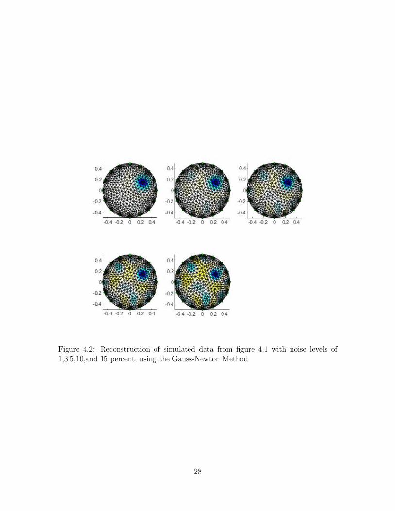
Figure 4.2: Reconstruction of simulated data from figure 4.1 with noise levels of1,3,5,10,and 15 percent, using the Gauss-Newton Method

28

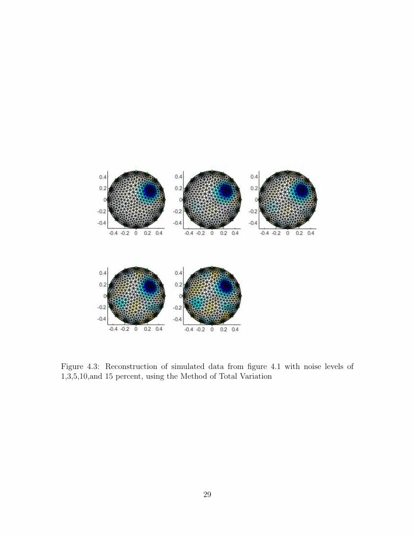
Figure 4.3: Reconstruction of simulated data from figure 4.1 with noise levels of1,3,5,10,and 15 percent, using the Method of Total Variation

29

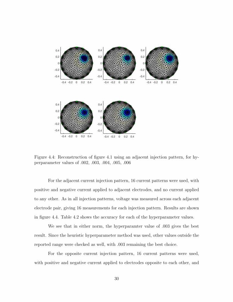
Figure 4.4: Reconstruction of figure 4.1 using an adjacent injection pattern, for hy-perparameter values of .002, .003, .004, .005, .006

For the adjacent current injection pattern, 16 current patterns were used, with

positive and negative current applied to adjacent electrodes, and no current applied

to any other. As in all injection patterns, voltage was measured across each adjacent

electrode pair, giving 16 measurements for each injection pattern. Results are shown

in figure 4.4. Table 4.2 shows the accuracy for each of the hyperparameter values.

We see that in either norm, the hyperparamter value of .003 gives the best

result. Since the heuristic hyperparameter method was used, other values outside the

reported range were checked as well, with .003 remaining the best choice.

For the opposite current injection pattern, 16 current patterns were used,

with positive and negative current applied to electrodes opposite to each other, and

30

Hyperparameter value .002 .003 .004 .005 .0061-norm .0257 .0183 .0199 .0201 .02162-norm .0468 .0417 .0500 .0526 .0561

Table 4.2: Values of the 1-norm and 2-norm using equation 4.1 corresponding tofigure 4.4, for various hyperparameter values in the adjacent current injection pattern

Hyperparameter value .002 .003 .004 .005 .0061-norm .0177 .0252 .0213 .0212 .02082-norm .0488 .0478 .0456 .0465 .0518

Table 4.3: Values of the 1-norm and 2-norm using equation 4.1 corresponding tofigure 4.5, for various hyperparameter values in the opposite current injection pattern

no current applied to any other. For example, a positive current was applied to

electrode 1 and a negative current was applied to electrode 9. Results are shown in

figure 4.5, and the accuracy given in table 4.3.

For the sinusoidal current injection pattern, a single current pattern was used,

with value of sin θ, where θ is the value of the angle of the electrode center, measured in

radians clockwise from the vertical. Results are shown in figure 4.6, and the accuracy

given in table 4.4. As discussed in chapter 2, the sinusoidal injection pattern in

expected to perform best, which it does.

Hyperparameter value .002 .003 .004 .005 .0061-norm .0177 .0186 .0176 .0180 .01812-norm .0485 .0430 .0486 .0488 .0489

Table 4.4: Values of the 1-norm and 2-norm using equation 4.1 corresponding to fig-ure 4.6, for various hyperparameter values in the sinusoidal current injection pattern

31

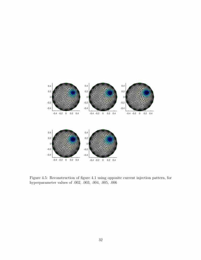
Figure 4.5: Reconstruction of figure 4.1 using opposite current injection pattern, forhyperparameter values of .002, .003, .004, .005, .006

32

Figure 4.6: Reconstruction of figure 4.1 using sinusoidal current injection pattern, forhyperparameter values of .002, .003, .004, .005, .006

33

Figure 4.7: Geometry of the forward model with two distinct inclusions.

Hyperparameter value .002 .003 .004 .005 .0061-norm .0361 .0364 .0400 .0377 .03802-norm .0726 .0720 .0875 .0802 .0807

Table 4.5: Values of the 1-norm and 2-norm using equation 4.1 corresponding tofigure 4.8, for various hyperparameter values using the Gauss-Newton Method

4.1.3 Double Inclusion

A model with two inclusions was created to compare the Gauss-Newton method

with the method of total variation for simulated data. The geometry was the same as

in section 4.1.1, with an additional inclusion at (-242mm,150mm). For both methods,

an adjacent current injection pattern was used. The geometry is shown in figure 4.7.

The results for the Gauss-Newton method are shown in figure 4.8, and the

accuracy described in table 4.5.

The results for the method of total variation are shown in figure 4.9, and the

34

Figure 4.8: Reconstruction of figure 4.7 with the Gauss-Newton method, for hyper-parameter values of .002, .003, .004, .005, .006

35

Figure 4.9: Reconstruction of figure 4.7 with the Total Variation method, for hyper-parameter values of .002, .003, .004, .005,.006

accuracy described in table 4.6, for the same hyperparameter values as used in the

Gauss-Newton method. However, the method of total variation had a best hyperpa-

rameter value of .001. The results of reconstruction using that hyperparameter value

are shown in figure 4.10. The accuracy of the reconstruction in figure 4.10 was .0281

for the 1-norm and .0651 for the 2-norm.

4.1.4 Limits of EIT Reconstruction

The limits of the EIT inverse problem reconstruction was investigated to ob-

serve when the inverse problem fails to recognize inclusions. First, multiple inclusions

were added to the simulated model. Next, one of the inclusion was decreased in size

36

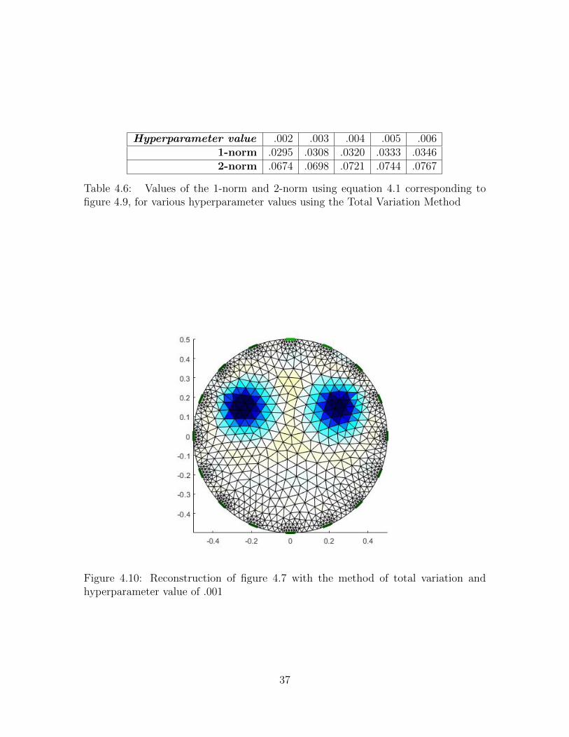
Hyperparameter value .002 .003 .004 .005 .0061-norm .0295 .0308 .0320 .0333 .03462-norm .0674 .0698 .0721 .0744 .0767

Table 4.6: Values of the 1-norm and 2-norm using equation 4.1 corresponding tofigure 4.9, for various hyperparameter values using the Total Variation Method

Figure 4.10: Reconstruction of figure 4.7 with the method of total variation andhyperparameter value of .001

37

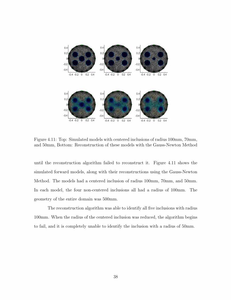
Figure 4.11: Top: Simulated models with centered inclusions of radius 100mm, 70mm,and 50mm, Bottom: Reconstruction of these models with the Gauss-Newton Method

until the reconstruction algorithm failed to reconstruct it. Figure 4.11 shows the

simulated forward models, along with their reconstructions using the Gauss-Newton

Method. The models had a centered inclusion of radius 100mm, 70mm, and 50mm.

In each model, the four non-centered inclusions all had a radius of 100mm. The

geometry of the entire domain was 500mm.

The reconstruction algorithm was able to identify all five inclusions with radius

100mm. When the radius of the centered inclusion was reduced, the algorithm begins

to fail, and it is completely unable to identify the inclusion with a radius of 50mm.

38

Figure 4.12: Recreation of figure 3.1 in EIDORS

4.2 Experimental Data

The experimental data obtained by Toa Ruan [12] and described in chapter 4

was reconstructed using the EIDORS inverse solver. Both the Gauss-Newton method

and the method of total variation were employed. First, the geometry, injection and

measurement patterns, and applied current as described in chapter 4 were supplied

to EIDORS. The background conductivity of 1.4 S/m was provided as the prior

information. Figure 3.1 shows an image of the experimental object. In order to

compare the accuracy of the reconstructions, the geometry in figure 3.1 was recreated

in EIDORS, and is shown in figure 4.12. This allows for the accuracy to be determined

by the equation 4.1.

39

Figure 4.13: Reconstruction of Experimental data using the Gauss-Newton method,for hyperparameter values of .0009, .001, .0011, .0012, .0013

The best hyperparameter values for the Gauss-Newton method and the method

of total variation differed by a factor of 100, which is expected given the given they use

different regularization terms. The results for the Gauss-Newton method are shown

in figure 4.13, and the accuracy described in table 4.7. The results for the method of

total variation are shown in figure 4.14, and the accuracy described in table 4.8.

It is important to note that the difference in colors between the two reconstruc-

tion images is misleading, as the images are scaled to different reference conductivities.

For example, the color white in figure 4.12 corresponds to a conductivity of 1.4S/m,

while color white in figure 4.14 corresponds to a different conductivity value, and the

color yellow corresponds to a conductivity of 1.4S/m. The location and the resolution

40

Hyperparameter value .0009 .001 .0011 .0012 .00131-norm .0650 .0614 .0584 .0559 .05392-norm .1747 .1749 .1750 .1750 .1749

Table 4.7: Values of the 1-norm and 2-norm using equation 4.1 corresponding tofigure 4.13, for various hyperparameter values using the Gauss-Newton method

Figure 4.14: Reconstruction of Experimental data using the method of total variation,for hyperparameter values of .14, .15, .16, .17, .18

Hyperparameter value .14 .15 .16 .17 .181-norm .1709 .1633 .1572 .1522 .14792-norm .2246 .2211 .2186 .2166 .2149

Table 4.8: Values of the 1-norm and 2-norm using equation 4.1 corresponding tofigure 4.14, for various hyperparameter values using the method of total variation

41

of the inclusion is what affects the accuracy.

42

Chapter 5

Conclusions and Discussion

Experimental data from the civil engineering field of cementitious materials

was reconstructed with two different reconstruction algorithms. The effect of altering

the current pattern was investigated using simulated data from EIDORS. Addition-

ally, methods of hyperparameter selection and the effect of altering the hyperparam-

eter were investigated with both simulated and experimental data.

The reconstruction of the experimental data was an absolute reconstruction.

Previously, this data was only reconstructed as a relative reconstruction, meaning

the accuracy of the conductivity distribution could not be determined. Here, two dif-

ferent reconstruction algorithms were utilized, and each was shown to have different

advantages. The Gauss-Newton reconstruction method produced less sharp images,

as seen in figure 4.13, but the norms as calculated with equation 4.1 were lower than

those of the total variation method, indicating better accuracy. The total variation

reconstruction method exhibited sharper images, as seen in figure 4.14. Thus, to-

tal variation reconstruction allowed for easier distinguishability between conductive

and non-conductive regions. Accuracy may be more important for some EIT appli-

cations while distinguishability may be more important in others. Thus, knowing

43

the strengths and weakness of each reconstruction method permits the researcher to

select the most fitting method for the problem at hand.

In section 4.1.1 the impact of noise was investigated. The results show that

increased noise affects both the reconstruction image quality and the accuracy of the

reconstruction. In section 4.1.2, adjacent, opposite, and sinusoidal injection patterns

were compared. As discussed previously, Cheney [3] found that the sinusoidal injec-

tion pattern performs the best. The results in section 4.1.2 support this claim, as

the norms in the sinusoidal injection pattern were slightly less than in the other two

patterns. Nevertheless, the reconstruction of all three patterns accurately identified

the location of the inclusion with good distinguishability. Since the sinusoidal pattern

is much more costly to implement experimentally, and only performed slightly better

than the other two patterns, using the adjacent or opposite injection pattern may be

more practical and suitable for many applications.

In each reconstruction, the heuristic hyperparameter selection method was

implemented. This involved first solving the inverse problem with a wide range of

hyperparameter values, from 10−1 to 10−5. Then, the best image was selected and

a smaller range of values used in the inverse problem calculation. Figure 2.1 shows

the instability of the reconstruction algorithm when a hyperparameter value of zero

is chosen. The Gauss-Newton algorithm fails to identify the inclusion due to the

ill-posed nature of the inverse problem when λ = 0. Even in the simulated data,

slight changes to the hyperparameter value have visible effects on the reconstruction

images. The reconstructions of experimental data in figure 4.13 show that a change

in hyperparemeter value of just .0001 drastically changes the inverse solution. Since

the choice of hyperparameter is so crucial to the inverse solution, development of

hyperparameter selection methods is crucial for the field of EIT.

44

5.1 Future Work

In this thesis, two reconstruction algorithms were evaluated. There are many

more reconstruction algorithms with various regularization, including statistical in-

version. The statistical inversion method will be used to reconstruct the experimental

data used in this thesis, and the results will be compared.

The data used in this thesis was from cementitious materials of the civil engi-

neering field. EIT has many other applications, the most prominent being the medical

field. Thus evaluation of these algorithms with medical data is important.

As discussed before, selection of the best hyperparameter is a crucial element

of reconstruction of EIT data, and there is no single method to guarantee optimal,

or consistent hyperparameter selection. Future work is needed to develope better, if

not optimal hyperparameter selection methods.

45

Appendices

46

Appendix A A Starting Guide to EIDORS

EIDORS runs in Matlab and uses NETGEN meshing software to create the

finite element mesh. Windows and linux are preferred operating systems for EIDORS.

EIDORS can also run in Octave, but it is much more difficult to arrange directories

correctly.

To use EIDORS for an EIT problem, the first step is to create the geometry

of the object. For simple geometries, there are built-in functions such as

”ng mk cyl models.” For more complex geometries, you must call Netgen directly.

Netgen objects are created by unions and intersections of basic shapes (spheres, rect-

angles, cylinders). The ”-maxh” command allows for different mesh sizes for different

parts of the object.

Next, define the electrode positions and shapes. These can be defined individ-

ually, but for most EIT problems, electrodes are equally spaced and of the same size,

so you can use the function ”ng mk cyl models(cyl shape, elec pos, elec shape).”

”cyl shape” has inputs height, radius. If height=0, then a 2D object is created.

”elec pos” has inputs n electrodes per plane, m number of planes, which will cre-

ate m rings of n equally spaced electrodes (for 2D, m=1). ”elec shape has inputs

width,height where height=0 produces circular electrodes. Both width=0 and

height=0 produce point electrodes. If point electrodes are used, the complete elec-

trode model is not used, as contact impedance would not exist.

Next, define the injection and measurement patterns with the function

”mk stim patterns.” this function has inputs number of electrodes, number of rings,

injection, measurement, options, amplitude. Injection has many options, including

adjacent, opposite, and trigonometric patterns. Measurement has the same options

as injection, with multiple measurements being made for each injection pattern. The

47

”Options” field is used to tell EIDORS not to measure on the current carrying elec-

trodes with the string ′no meas current′. ”Amplitude” is the applied current in

Amps.

Lastly, set the conductivity of the geometry. First, set the background conduc-

tivity using ”mk image”, which has inputs fwdmodel, conductivity. For nonhomo-

geneous regions, use ”elem select” to define different regions, and call ”elem data”

to change the conductivity of that region.

Now, all of the aspects of the forward problem are set, so use ”fwd solve” to

solve for the voltages on the electrodes, which is the simulated data.

For the inverse model, set the geometry, injection and measurement patterns,

solver, hyperparameter value, and background conductivity (prior). Set

”imdl.fwd model = fmdl” to use the same geometry and patterns as was used in

the forward model. The function ”inv solve” solves the inverse problem, with inputs

invmodel, voltage vector. The output is the reconstructed image, and a vector of

conductivity values. The accuracy of the reconstruction can be obtained by comparing

the reconstructed image with the true conductivity distribution.

If you run into problems using EIDORS, the first step is to check both the

EIDORS and NETGEN documentation for troubleshooting, [1] [13]. If problems

persist, search the EIDORS mailing list by keyword. If more help is needed, you can

send an email to the developers’ mailing list; they usually are prompt in responding.

48

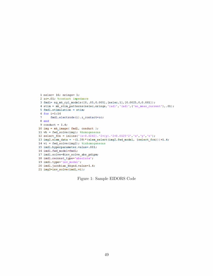
Figure 1: Sample EIDORS Code

49

Bibliography

[1] A. Adler and W. Lionheart. Uses and abuses of EIDORS: An extensible softwarebase for EIT. Physiological Measurement, 27(5):S25–S42, 2006.

[2] A. Borsic. Regularisation Methods for Imaging from Electrical Measurements.PhD thesis, Oxford Brooks University, 2002.

[3] M. Cheney and D. Isaacson. Distinguishability in impedance imaging. Transac-tions on Biomedical Engineering, 39(8):852–860, 1992.

[4] M. Cheney, D. Isaacson, J. Newell, S. Simske, and J. Goble. Noser: An algo-rithm for solving inverse conductivity problem. International Journal of ImagingSystems and Technology, 2:66–75, 1990.

[5] M. Cheney, D. Isaacson, and J.C. Newell. Electrical impedance tomography.Society for Industrial and Applied Mathematics, 41(1):85–101, 2004.

[6] R. Cholathat, L. Ge, X. Li, and C. Rizos. Monitoring geologic carbon sequestra-tion with radar remote sensing. In The 10th Australian Space Science Conference,pages 187–198. National Space Society of Australia Ltd, September 2010.

[7] E. Demidenko, A. Borsic, Y. Wan, R.J. Halter, and A. Hartov. Statistical esti-mation of eit electrode contact impedance using a magic toeplitz matrix. IEEETransactions on Biomedical Engineering, 58(8):2194–2201, 2011.

[8] B.M. Graham. Enhancements in Electrical Impedance Tomography Reconstruc-tion of 3D Lung Imagining. PhD thesis, University of Ottawa, April 2007.

[9] B.M. Graham and A. Adler. Objective selection of hyperparameter for EIT.Physiological Measurement, 27(5):S65–S79, 2006.

[10] S. I. Kabanikhin. Definitions and examples of inverse and ill-posed problems.Journal of Inverse and Ill-posed Problems, 16:317–357, 2008.

[11] E.K. Oware, S.M.J. Moysey, and T. Khan. Physically based regularization of hy-drogeophysical inverse problem for improved imaging of process-driven systems.Water Resources Research, 49:1–10, 2013.

50

[12] T. Ruan. Development of an Automated Electrical Impedance Tomography Sys-tem and Its Implementation in Cementitious Materials. PhD thesis, ClemsonUniversity, August 2016.

[13] J. Schoberl. Netgen-4.x. https://sourceforge.net/projects/netgen-mesher, March2010.

[14] E. Somersalo, M. Cheney, and D. Isaacson. Existence and uniqueness for elec-trode models for electric current computed tomography. SIAM Journal on Ap-plied Mathematics, 52(4):1023–1040, 1992.

51