Lidsey SWMP Modelling reports

Lidsey SWMP Appendix D - Lidsey SWMP Modelling Report

July 2014


Atkins Appendix D - Lidsey SWMP Modelling Report | Version 1.0 | 1 July 2014

Notice This report has been prepared as part of West Sussex County Council’s responsibilities under the Flood Water Management Act 2010. It is intended to provide context and information to support the delivery of the local flood risk management strategy and should not be used for any other purpose.

Atkins assumes no responsibility to any other party in respect of or arising out of or in connection with this document and/or its contents.

This document has 31 pages including the cover.

Document history Job number: Document ref:

Revision Purpose description Originated Checked Reviewed Authorised Date

Rev 1.0 Lidsey SWMP – Appendix D

Will Rust Matt McDonald

Adam Cambridge

Matt McDonald

July 2014

Rev 2.0 Partner comments incorporated.

Will Rust Matt McDonald

Matt McDonald

August 2014


Atkins Appendix D - Lidsey SWMP Modelling Report | Version 1.0 | 1 July 2014

Table of Contents Chapter Pages 1. Introduction 5 2. Model Build 6 2.1. Approach 6 2.2. Model Extent 6 2.3. Model Detail 7 2.4. The 1D Sewer System 8 2.5. The 1D River System 10 2.6. The 1D Groundwater Model 11 2.7. The 2D Model 15 3. Model Verification 17 3.1. Short Term Flow Survey 17 3.2. Model Performance 21 4. Design Storm events 23 5. Model Simulation 27 5.1. Timestep and Runtimes 27 5.2. Stability 27 6. Conclusions and Recommendations 28 7. References 29

Tables Table 2-1 1D Structures Represented in the River Systems 10 Table 2-2 Fixed Runoff Values for 2D Infiltration 16 Table 3-1 Summary of Flow Survey Results 17 Table 3-2 Summary of Rain Gauge Locations 18 Table 4-1 Design Groundwater Levels 24

Figures Figure 2-1 Study Boundary and Model Extent 6 Figure 2-2 Groundwater Catchment and Routing Model 12 Figure 2-3 Modelled Groundwater Response at the Barn Rise Boreholes 12 Figure 2-4 Modelled Groundwater Response at the Woodgate Borehole 13 Figure 2-5 Modelled Groundwater Response at the Shripney Borehole 13 Figure 2-6 Schematic of Linkages from the Groundwater Model to the Sewer System 14 Figure 2-7 LiDAR Extent and Resolutions within the Model Boundary 15 Figure 3-1 Locations of Short Term Rain Gauges and Flow Monitors 19 Figure 3-2 Measured Rainfall During the Flow Survey 20 Figure 3-3 Adopted Evaporation Data 21 Figure 3-5 Foul Sewer Simulation Results for Storm C at FM09 in Barnham Town Centre. Red - Measured / Green – Modelled 21 Figure 3-7 Simulated Infiltration into Manhole SU95047403 22 Figure 4-1 Typical Design Storm Rainfall Profiles 23 Figure 4-2 Relationship Between Rife Baseflow to Barn Rise Groundwater Level 24 Figure 4-3 Comparison of Predicted 1 in 100 Year Flood Extents With Recorded Historical Flooding 25 Figure 4-4 Comparison of Predicted 1 in 30 Year Flood Extents with the EA’s Flood Maps for Surface Water (2010 & 2014) 26


Atkins Appendix D - Lidsey SWMP Modelling Report | Version 1.0 | 1 July 2014 5

1. Introduction During the Lidsey SWMP an InfoWorks ICM model was developed to better understand localised flood mechanisms and determine the flood risk to property and people in the catchment. This report summarises the development of the InfoWorks ICM model which represents the following in the Lidsey catchment:

• overland flows, • river channels (albeit coarsely represented), • sewer systems, • interactions with the coast (tides), and • groundwater system (using a novel approach developed as part of this commission).

The representation of these systems in an integrated model was deemed necessary, as it is known that historical floods have largely been in response to storms falling on a catchment that already has elevated groundwater levels which has reduced the headroom in the sewer systems as a result of infiltration.



2. Model Build 2.1. Approach The Lidsey catchment requires an approach that simulates the relative timings of rainfall falling on urban and rural surfaces, flows in rivers, interactions with the coast (tides), and groundwater rebound. While historically the different aspects of the hydrological system have been treated as separate entities, the technical tools used to represent and understand the flooding regime have begun to allow greater integration of the river, coastal, above ground, groundwater, and sewer environments. These are relatively new techniques that are more commonly known as Integrated Urban Drainage (IUD) modelling approaches that have partly been driven by the events that unfolded during the summer floods of 2007, and the “Making Space for Water”, “Foresight Future Flooding”, and “Pitt Review” consultations.

For the purposes of this study it was deemed appropriate to adopt InfoWorks ICM (version 4.5), as it is able to simulate all of the necessary systems apart from groundwater in an integrated manner. The simulation of groundwater, and its affect on river and sewer performance, is an area of ongoing research, but was undertaken using the most appropriate aspects of InfoWorks ICM so as to generate groundwater volume and its subsequent routing. Further details are provided in 2.6.

Central to the approach has been to pin back assumptions and use the most appropriate technique for the catchment processes at hand, for example, using 2D infiltration methods for generating runoff.

2.2. Model Extent The study boundary for the Lidsey SWMP and the extent of the InfoWorks ICM model is shown in Figure 2-1 below. The InfoWorks ICM model boundary is significantly larger than the study boundary because the model explicitly represents the groundwater system for the catchment. The modelling extent consists of:

• 2 x wastewater catchments – Lidsey (LIDS) and the Ford catchments (FORD), • 5 x rivers – Barnham Rife, Lidsey Rife, Ryebank Rife, and Aldingbourne Rife • The Bognor Regis coastline, and • The South Downs chalk aquifer and other associated geology e.g. London Clay

The model boundary was delineated using panorama topographic contours and the major watercourses, given that this will drive infiltration into the groundwater system, as well as loss.

Figure 2-1 Study Boundary and Model Extent



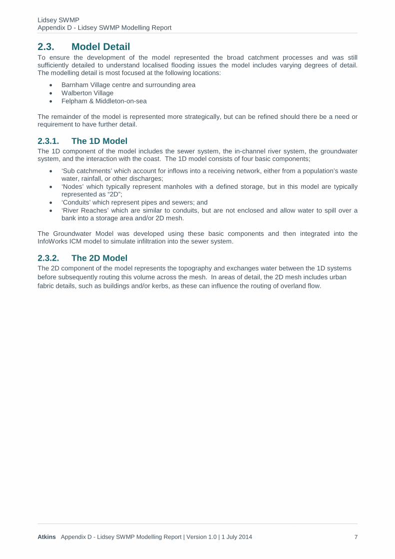
2.3. Model Detail To ensure the development of the model represented the broad catchment processes and was still sufficiently detailed to understand localised flooding issues the model includes varying degrees of detail. The modelling detail is most focused at the following locations:

• Barnham Village centre and surrounding area • Walberton Village • Felpham & Middleton-on-sea

The remainder of the model is represented more strategically, but can be refined should there be a need or requirement to have further detail.

2.3.1. The 1D Model The 1D component of the model includes the sewer system, the in-channel river system, the groundwater system, and the interaction with the coast. The 1D model consists of four basic components;

• ‘Sub catchments’ which account for inflows into a receiving network, either from a population’s waste water, rainfall, or other discharges;

• ‘Nodes’ which typically represent manholes with a defined storage, but in this model are typically represented as “2D”;

• ‘Conduits’ which represent pipes and sewers; and • ‘River Reaches’ which are similar to conduits, but are not enclosed and allow water to spill over a

bank into a storage area and/or 2D mesh.

The Groundwater Model was developed using these basic components and then integrated into the InfoWorks ICM model to simulate infiltration into the sewer system.

2.3.2. The 2D Model The 2D component of the model represents the topography and exchanges water between the 1D systems before subsequently routing this volume across the mesh. In areas of detail, the 2D mesh includes urban fabric details, such as buildings and/or kerbs, as these can influence the routing of overland flow.



2.4. The 1D Sewer System

2.4.1. The Sewer System The sewer system within the study area was modelled as 1D conduits using existing InfoWorks CS models and asset data. The foul sewer system is largely based on Southern Water’s existing verified InfoWorks CS models and the storm sewer system is largely based on Southern Water’s asset data. The land and highway drainage systems were built into the InfoWorks ICM model using data and mapping provided by Arun District Council (ADC) and West Sussex County Council (WSCC).

2.4.1.1. The Foul Sewer System The Lidsey Catchment (LIDS)

The Lidsey (LIDS) sewer system model was verified against a winter short term flow survey which was conducted between January and May 2012. Two of the three WaPUG criteria storm events captured by the survey were late April 2012, are known to have not occurred during worst-case groundwater conditions for the catchment.

A delayed rainfall induced inflow was observed during the verification events, but this could not effectively recreate a surcharged state at Lidsey Wastewater treatment works (WTW), which was measured during the flow survey. To achieve a ‘forced’ verification fit, a level file was applied to the works with the measured level data.

The Ford Catchment (FORD) – Bognor Regis model (BOGN)

The Bognor Regis (BOGN) sewer system model represents only a portion of the larger Ford sewerage catchment. This was calibrated against a winter short term flow survey and achieved a satisfactory level of verification.

Sub catchment Flows

The existing foul sewer system models represent contributing area as lumped areas containing multiple houses (i.e. rainfall from roofs, roads, hard-standing and misconnected surfaces, and wastewater contributions from the population and commercial premises), which is standard practice for a 1D network model. For the purposes of this project, it was necessary to redefine these contributing sub catchments, so that each sub catchment only represented a single property’s rainfall and foul contribution to the network and/or soakaway, as 2D rainfall-runoff was used for permeable and other impermeable (road and hard standing) contributions.

2.4.1.2. The Storm Sewer System None of the storm sewer system and highway/land drainage network was represented in the existing hydraulic models for the Lidsey and Bognor Regis catchments. Details of the Southern Water’s storm sewer assets were imported into InfoWorks ICM, and details of private drainage assets were digitised from land/highway drainage maps provided by ADC and WSCC.

In some areas of the study area, parts of sewer network were found to be isolated from the main systems, i.e. not connected to any other part of the network. None of these isolated parts of network were found to be of significance to the drainage of surface water or to flooding and were not represented, but can be in the future if required.

2.4.2. Inferences Where there was missing data in the sewer systems and the land drainage network data, details were inferred using the standard inference tools within InfoWorks ICM and in conjunction with engineering judgement. The following inferences were used:

• All ground levels of sewer manholes were inferred from the DTM. • Invert levels have been inferred between known invert levels, or the DTM ground level at discharge

points. • Pipe diameters have been inferred from nearby conduits. • Headlosses have been applied to manhole junctions.



2.4.3. Property Soakaway Systems With approximately 60% of property roofs draining to soakaways it was considered necessary to explicitly represent these systems within the Infoworks ICM model. Soakaways have been represented as storage ‘nodes’ with sub catchment roofs attached and SUDS parameters were applied for the:

• ‘Base Area’, • ‘Porosity’ and • ‘Infiltration loss coefficient.

This setup effectively allows roof runoff to be routed to the soakaways, stored, and then subsequently infiltrated. There is no connection to the groundwater model, as the small amount of contribution from these surfaces was not considered to be significant in respect to groundwater rebound. If the roof runoff exceeds the capacity of the soakaway, flows spill onto the 2D surface and can also receive flow from the 2D surface. The later is a limitation and will yield conservative predictions in respect to soakaway performance.

The SUDS parameters, which are based on parameters provided in the SuDS manual, have been globally applied and represent typically values. These can be refined with soakway tests where and when required.



2.5. The 1D River System

2.5.1. Open Channels The Environment Agency’s Detailed River Network (DRN) dataset was used to determine what watercourses needed to be represented for interactions with the sewer system. The remaining open channels have been represented using the 2D mesh using InfoWorks ICM’s Terrain Sensitive Meshing.

It is important to highlight that the river system does not include any river survey (including structures) and does then only purely represent interaction. This strategic and coarse approach was used, as it was understood that the EA would refine and develop this area of the InfoWorks ICM model in undertaking a similar and subsequent study.

Runoff into the river system is generated by the 2D Mesh and through the use of infiltration surfaces. Rural-runoff was simulated using a fixed percentage of 30% to be in line with the approach being adopted by the EA. Baseflows have been represented coarsely as 0.1m³/s inflows per river reach to ensure river channels have flow, but this obviously requires review and revision in subsequently more detailed studies of the river system.

2.5.2. Structures No structural information of river structures was available, so site visits were undertaken to obtain details for inclusion in the InfoWorks ICM model e.g. culvert inlets / outlets, headwalls, weirs, bridges and tidal gates. The geometry of these structures were measured on site (where possible) and taken from available drainage maps and/or LiDAR data. Table 2-1 lists the structures that were built into the InfoWorks ICM model.

Table 2-1 1D Structures Represented in the River Systems

ID Location Structure NGR Description 1 Barnham Lane Culvert 496037, 105704 Circular culvert 2 Lidsey WTW Culvert 494292, 103299 Rectangular culvert 3 Woodgate Culvert 494341, 104332 Rectangular culvert 4 Highground Lane Culvert 495616, 103745 Rectangular culvert 5 Eastergate Lane Culvert 469411, 106111 Circular Culvert 6 South of Eastergate Lane Culvert 496498, 106087 Circular Culvert to Village pond 7 Eastergate Lane 496558, 106089 Circular Culvert 8 Barnham Road Bridge Bridge 496166,104536 Box Culvert 9 Walberton Lane Culvert 496336, 106375 Circular Culvert 10 North of Spinney Walk Culvert 495895, 105047 Circular Culvert 11 Barnham Road Culvert 495988, 104389 2 x Box culverts under railway 12 Worms Lane Culvert 497849, 101403 Box Culvert 13 Yapton Road Culvert 497591, 101575 Box Culvert

14 Bognor Regis Butlins Culvert 494733, 99183 Outfall to sea 15 Bognor Regis Butlins Culvert 494588, 99400 Box Culvert 16 A259 Culvert 494620, 99988 Box Culvert 17 South of Marshalls Close Culvert 495871, 104170 Box culvert 18 Lake Lane Culvert 496384, 104681 Circular culvert 19 Lake Lane Culvert 496440, 104687 Circular culvert 20 Lake Lane Culvert 496473, 104695 Circular Culvert 21 Hill Lane Culvert 496406, 103731 Circular Culvert 22 Mill Lane Culvert 496681, 106123 Circular Culvert 23 The Street Culvert 496638, 106093 2 x Circular Culvert 24 Upper Bognor Road Bridge 494581, 99517 Tidal Gate 25 Upper Bognor Road Bridge 494574, 99476 26 Felpham Way Bridge 494559, 99916 27 South of Barnham Bridge 495006, 103462 Railway Bridge 28 South of Woodgate Bridge 494913, 102773 Railway Bridge



2.6. The 1D Groundwater Model

2.6.1. Introduction In order to prepare surface water flood risk maps that represented the effect of infiltration reducing the headroom in the sewer systems it was necessary to incorporate a groundwater component into the InfoWorks ICM model. It is important to highlight that whilst this novel approach was taken, groundwater modelling is a complex technical area, and the groundwater model developed is a mass representation of the groundwater system focusing on the Barnham and Middleton-on-Sea areas of the study area.

The groundwater model was developed in two parts. First, a model was developed to convert rainfall to groundwater inflow (volume) and rebound. Secondly, a model was developed to route this volume to the coast, so that variations in level across the domain could be represented. Both are briefly summarised below.

2.6.2. Groundwater Model Setup A contributing catchment was delineated using panorama topographic contours and the major watercourses (refer to Figure 2-2), given that this will drive infiltration into the groundwater system. The catchment was then simulated with InfoWorks ICM’s groundwater infiltration model to allow rainfall to be converted to volume and rebound. The groundwater infiltration model was setup using appropriate soil and ground condition parameters and was calibrated to a year’s worth of borehole data (August 2010 to July 2011) recorded at Barn Rise using rainfall and evaporation data (MORESCS).

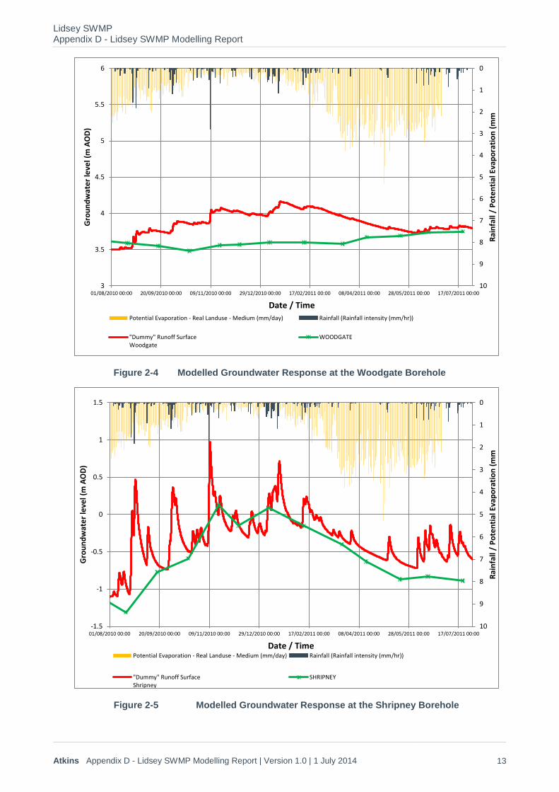
The predicted groundwater inflow from the ground infiltration model setup was then used to configure a “dummy” runoff setup to simplify its incorporation into the broader InfoWorks ICM model. The “dummy”, or configured groundwater runoff surface, was then applied to a permeable network arrangement (refer to Figure 2-2 below), which simulates the movement of water using the principles of Darcy’s Law to allow predicted groundwater levels to be routed to the coast. This mass representation of groundwater routing across the catchment was used to simulate varying levels in the groundwater system and was configured to re-create levels at the Barn Rise boreholes (Figure 2-3) and at two downstream bore holes – Woodgate (Figure 2-6) and Shripney (Figure 2-7).

The conversion of rainfall to groundwater volume at the Barns Rise boreholes was considered appropriate for the purposes of this commission, as the model is effectively converting 85% of the total rainfall volume to groundwater inflow with the remainder (15%) effectively converted to catchment runoff, which is in line with the approximate SPRHOST for the catchment (20 to 30%). The re-bound (Figure 2-3) of this volume within the model was considered appropriate because the model is following the general rises and falls in borehole data, which when subsequently applied to the routing model is re-producing levels recorded at Shripney (Figure 2-7), but obviously not at Woodgate (Figure 2-6). Given that the Shripney borehole is downstream of Woodgate and the re-bound is likely to follow a similar pattern throughout the system, the data recorded at Woodgate is likely to be in error and it is recommended that this be reviewed in taking forward the model. Improvements such as this should be undertaken using a fuller groundwater model and indeed a refined spatial representation of rainfall given this directly affects the conversion of rainfall to groundwater inflow.

It is worth noting that the hydraulic representation of the groundwater does not distinguish between the chalk aquifer and the perched water table in the clay (brickearth) geological layers.



Figure 2-2 Groundwater Catchment and Routing Model

Figure 2-3 Modelled Groundwater Response at the Barn Rise Boreholes

0

1

2

3

4

5

6

7

8

9

107.00

7.50

8.00

8.50

9.00

9.50

10.00

01/08/2010 20/09/2010 09/11/2010 29/12/2010 17/02/2011 08/04/2011 28/05/2011 17/07/2011

Rain

fall

/ Po

tent

ial E

vapo

ratio

n (m

m

Gro

und

Stor

e Le

vel (

m A

OD)

Date / Time Potential Evaporation - Real Landuse - Medium (mm/day) Rainfall (Rainfall intensity (mm/hr))

Barn Rise - BH1 (m AOD) Barn Rise - BH3 (m AOD)

Barn Rise - BH4 (m AOD) "Dummy" Runoff SurfaceBarn Rise

Woodgate Borehole

Shripney Borehole

Barn Rise Boreholes



Figure 2-4 Modelled Groundwater Response at the Woodgate Borehole

Figure 2-5 Modelled Groundwater Response at the Shripney Borehole

0

1

2

3

4

5

6

7

8

9

103

3.5

4

4.5

5

5.5

6

01/08/2010 00:00 20/09/2010 00:00 09/11/2010 00:00 29/12/2010 00:00 17/02/2011 00:00 08/04/2011 00:00 28/05/2011 00:00 17/07/2011 00:00

Rain

fall

/ Po

tent

ial E

vapo

ratio

n (m

m

Gro

undw

ater

leve

l (m

AO

D)


"Dummy" Runoff SurfaceWoodgate

WOODGATE

0

1

2

3

4

5

6

7

8

9

10-1.5

-1

-0.5

0

0.5

1

1.5

01/08/2010 00:00 20/09/2010 00:00 09/11/2010 00:00 29/12/2010 00:00 17/02/2011 00:00 08/04/2011 00:00 28/05/2011 00:00 17/07/2011 00:00

Rain

fall

/ Po

tent

ial E

vapo

ratio

n (m

m

Gro

undw

ater

leve

l (m

AO

D)


"Dummy" Runoff SurfaceShripney

SHRIPNEY



2.6.3. Linking the Groundwater Model to the Sewer network Given that some areas of the sewer system are likely to be more resilient to infiltration than others and applying the groundwater model in a blanket fashion would be too simplistic, an “Infiltration and Inflow” investigation (I&I) was conducted on the sewer system. The I&I investigation identified locations of groundwater ingress in the sewer system (mainly in the northern area of the catchment – Barnham – with very little found in the Middleton and Bognor Regis areas), which was then used to define where the groundwater model should applied to. However, as the groundwater model was only configured to represent the system up to the Barn Rise boreholes it can only, and has, been applied to the network where ground levels are less than or equal to 9.0m AOD.

Connections between the groundwater model and the 1D sewer network have been represented in InfoWorks ICM using theoretical flap valves, so that the connections purely represent infiltration rather exfiltration too. This was considered appropriate, as the project is concerned with the groundwater system and infiltration reducing the headroom in the sewer system. The connection of the groundwater model to the sewer system is summarised in the schematic provided in Figure 2-6 below.

The connections have been verified to a short term flow survey, which is described in section 3.

Figure 2-6 Schematic of Linkages from the Groundwater Model to the Sewer System



2.7. The 2D Model

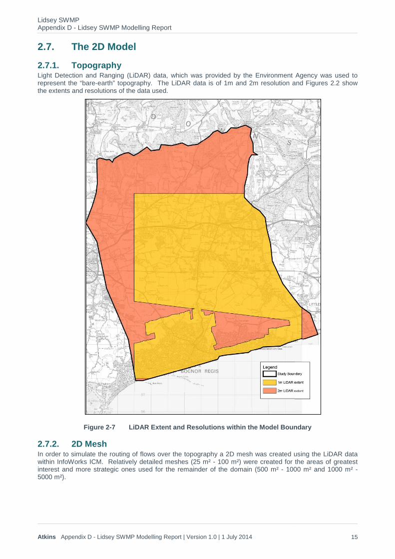
2.7.1. Topography Light Detection and Ranging (LiDAR) data, which was provided by the Environment Agency was used to represent the “bare-earth” topography. The LiDAR data is of 1m and 2m resolution and Figures 2.2 show the extents and resolutions of the data used.

Figure 2-7 LiDAR Extent and Resolutions within the Model Boundary

2.7.2. 2D Mesh In order to simulate the routing of flows over the topography a 2D mesh was created using the LiDAR data within InfoWorks ICM. Relatively detailed meshes (25 m² - 100 m²) were created for the areas of greatest interest and more strategic ones used for the remainder of the domain (500 m² - 1000 m² and 1000 m² - 5000 m²).



2.7.3. Building Representation Buildings have been represented as porous polygons based on Mastermap mapping. The porous polygons include a 150mm property threshold. This is a strategic approach to the representation of property thresholds, which is appropriate for the strategic nature of this project. In the future this can be refined to the specific modelling needs and justification.

2.7.4. Kerbs Kerbs along roads have been represented using ‘breaklines’, which effectively splice the generation of the 2D mesh. Kerb alignments were taken from the OS Mastermap mapping and are largely used in areas of detail.

2.7.5. Surface Roughness The Roughness of the surface was represent using an appropriate “Manning’s ‘n’ coefficient. Urban areas being represented with a coefficient of 0.02 and non-urban areas being represented with a coefficient of 0.06. This is a strategic approach to the representation of surface roughness, which is appropriate for the strategic nature of this project. In the future this can be refined.

2.7.6. Surface Infiltration Losses from the land surface as a result of infiltration have been represented using a fixed percentage runoff based on a conservative SPRHOST for the catchment and to be in line with the approach that is to be used by the EA in a subsequent study. It is, however, recommended that this be reviewed, as this will not account for seasonal variation of catchment wetness and a Horton infiltration surface be developed and used.

2D Infiltration surfaces have been inferred from OS MasterMap land use types. Geometry objects from the MasterMap GIS layer have been simplified before being imported into the model: unnecessary vertices removed from polygons and adjoining polygons of the same land use type have been merged into single polygons. This process avoids and limits excessive number of polygon 2D infiltration surfaces which can inhibit simulation performance.

Table 2-1 shows the runoff parameters classified by OS MasterMap land uses.

Table 2-2 Fixed Runoff Values for 2D Infiltration

Topo Area Type Fixed Percentage Runoff value

Natural Land (Greenfield Runoff) 30%

Multi-Purpose 40%

Manmade 100%

Roads / Rail 100%



3. Model Verification 3.1. Short Term Flow Survey

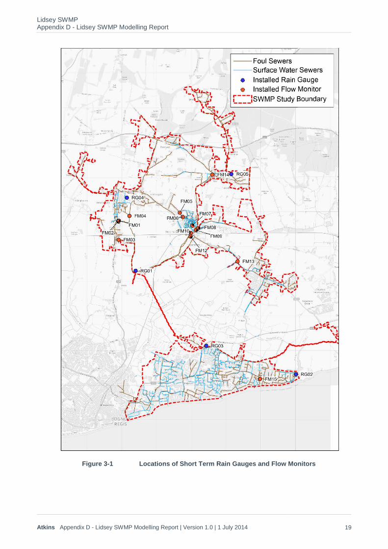
3.1.1. Introduction As part of the SWMP commission a short term flow survey was undertaken on the Lidsey wastewater catchment from the 22th March to the 24th of April 2013. This consisted of 15 x flow gauges within the sewer network and 5 x Rain gauges to allow the InfoWorks ICM model to be verified. It should, however, be noted that the river system within the InfoWorks ICM model was not verified, as it is understood that this will be undertaken by the EA in taking forward the project and model.

3.1.2. Flow Survey Data Fifteen Flow monitors were installed in the foul and storm system sewers in the study area. Table 3-1 below summarises the quality and coverage of this flow data and Figure 3-1 shows the location of the flow monitors.

Table 3-1 Summary of Flow Survey Results

Flow Monitor

Location Manhole

Pipe Diameter

Upstream (US) /

Downstream (DS)

Location Flow data

quality Comment

FM01 SU93049703 300 DS Elmcroft Place Moderate Data missing from 22/03/2013 to 10/04/2013

FM02 SU93048754 675 DS Elmcroft Place Good

FM03 SU9304810D 225 DS Woodgate Road Moderate

Strong signal from unknown pumped inflow

FM04 SU94042801 300 DS St Richards Road Moderate

Data missing between 06/04/2013 and 12/04/2013

FM05 SU95046901 225 US Elm Grove Moderate Data missing between 23/03/2013 and 28/03/2013

FM06 SU95047852 225 US Oriel Close Good

FM07 SU9604065X 450 US Farnhurst Road Good

FM08 SU96041555 375 DS Lake Lane Good FM09 SU96041401 375 US Lake Lane Good

FM10 SU95049302 300 US Barnham Road Good Data missing 22/03/2013 and 05/04/2013

FM11 Monitor Malfunction FM12 SU95049213 525 US Marshall Close Poor Possible ragging FM13 SU97033550 300 US Yapton Road Good

FM14 SU96066002 300 DS Barnham Lane Good Data unusable between 11/04/2013 and 24/04/2013

FM15 SU97009104 150 DS Rose Avenue Poor Strong signal from unknown pumped inflow



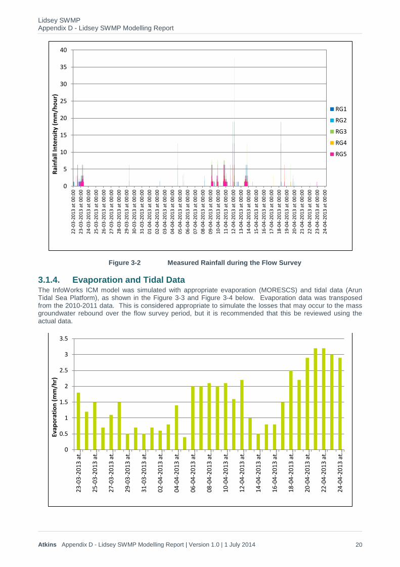
3.1.3. Rainfall Five tipping-bucket rain gauges were installed across the study area over the short term flow survey period, as shown in Figure 3-2. Three storm events and two dry weather flow days met the WaPUG criteria for verification storms:

• Storm Event 1: 9/04/2013 • Storm Event 2: 10/04/2013 • Storm Event 3: 12/04/2013 • DWF 1: 02/04/2013 • DWF 2: 07/04/2013

Although three storms were selected as meeting WaPUG verification storm criteria, only STORM C was used as the primary focus for verification, as this was the largest storm and appropriate verification to this would ensure that the model would be suitable for its purpose – design event storm modelling. Storms A and B showed significantly lower rainfall intensities and only marginally passed WaPUG criteria for verification storms.

Table 3-2 Summary of Rain Gauge Locations

Rain Gauge Location RG01 Lidsey WTW RG02 The Hard Sewage Pumping Station RG03 Acorn Fencing, Flansham Lane RG04 Westergate Community School RG05 Amber, The Street



Figure 3-1 Locations of Short Term Rain Gauges and Flow Monitors



Figure 3-2 Measured Rainfall during the Flow Survey

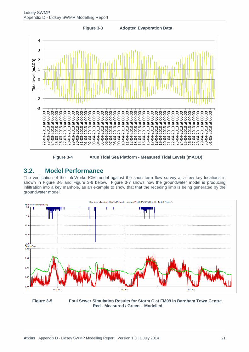
3.1.4. Evaporation and Tidal Data The InfoWorks ICM model was simulated with appropriate evaporation (MORESCS) and tidal data (Arun Tidal Sea Platform), as shown in the Figure 3-3 and Figure 3-4 below. Evaporation data was transposed from the 2010-2011 data. This is considered appropriate to simulate the losses that may occur to the mass groundwater rebound over the flow survey period, but it is recommended that this be reviewed using the actual data.

0

5

10

15

20

25

30

35

40

22-0

3-20

13 a

t 00:

0023

-03-

2013

at 0

0:00

24-0

3-20

13 a

t 00:

0025

-03-

2013

at 0

0:00

26-0

3-20

13 a

t 00:

0027

-03-

2013

at 0

0:00

28-0

3-20

13 a

t 00:

0029

-03-

2013

at 0

0:00

30-0

3-20

13 a

t 00:

0031

-03-

2013

at 0

0:00

01-0

4-20

13 a

t 00:

0002

-04-

2013

at 0

0:00

03-0

4-20

13 a

t 00:

0004

-04-

2013

at 0

0:00

05-0

4-20

13 a

t 00:

0006

-04-

2013

at 0

0:00

07-0

4-20

13 a

t 00:

0008

-04-

2013

at 0

0:00

09-0

4-20

13 a

t 00:

0010

-04-

2013

at 0

0:00

11-0

4-20

13 a

t 00:

0012

-04-

2013

at 0

0:00

13-0

4-20

13 a

t 00:

0014

-04-

2013

at 0

0:00

15-0

4-20

13 a

t 00:

0016

-04-

2013

at 0

0:00

17-0

4-20

13 a

t 00:

0018

-04-

2013

at 0

0:00

19-0

4-20

13 a

t 00:

0020

-04-

2013

at 0

0:00

21-0

4-20

13 a

t 00:

0022

-04-

2013

at 0

0:00

23-0

4-20

13 a

t 00:

0024

-04-

2013

at 0

0:00

Rain

fall

Inte

nsity

(mm

/hou

r)

RG1

RG2

RG3

RG4

RG5

0

0.5

1

1.5

2

2.5

3

3.5

23-0

3-20

13 a

t…

25-0

3-20

13 a

t…

27-0

3-20

13 a

t…

29-0

3-20

13 a

t…

31-0

3-20

13 a

t…

02-0

4-20

13 a

t…

04-0

4-20

13 a

t…

06-0

4-20

13 a

t…

08-0

4-20

13 a

t…

10-0

4-20

13 a

t…

12-0

4-20

13 a

t…

14-0

4-20

13 a

t…

16-0

4-20

13 a

t…

18-0

4-20

13 a

t…

20-0

4-20

13 a

t…

22-0

4-20

13 a

t…

24-0

4-20

13 a

t…

Evap

orat

ion

(mm

/hr)



Figure 3-3 Adopted Evaporation Data

Figure 3-4 Arun Tidal Sea Platform - Measured Tidal Levels (mAOD)

3.2. Model Performance The verification of the InfoWorks ICM model against the short term flow survey at a few key locations is shown in Figure 3-5 and Figure 3-6 below. Figure 3-7 shows how the groundwater model is producing infiltration into a key manhole, as an example to show that that the receding limb is being generated by the groundwater model.

Figure 3-5 Foul Sewer Simulation Results for Storm C at FM09 in Barnham Town Centre. Red - Measured / Green – Modelled

-3

-2

-1

0

1

2

3

422

-03-

2013

at 0

0:00

23-0

3-20

13 a

t 00:

0024

-03-

2013

at 0

0:00

25-0

3-20

13 a

t 00:

0026

-03-

2013

at 0

0:00

27-0

3-20

13 a

t 00:

0028

-03-

2013

at 0

0:00

29-0

3-20

13 a

t 00:

0030

-03-

2013

at 0

0:00

31-0

3-20

13 a

t 00:

0001

-04-

2013

at 0

0:00

02-0

4-20

13 a

t 00:

0003

-04-

2013

at 0

0:00

04-0

4-20

13 a

t 00:

0005

-04-

2013

at 0

0:00

06-0

4-20

13 a

t 00:

0007

-04-

2013

at 0

0:00

08-0

4-20

13 a

t 00:

0009

-04-

2013

at 0

0:00

10-0

4-20

13 a

t 00:

0011

-04-

2013

at 0

0:00

12-0

4-20

13 a

t 00:

0013

-04-

2013

at 0

0:00

14-0

4-20

13 a

t 00:

0015

-04-

2013

at 0

0:00

16-0

4-20

13 a

t 00:

0017

-04-

2013

at 0

0:00

18-0

4-20

13 a

t 00:

0019

-04-

2013

at 0

0:00

20-0

4-20

13 a

t 00:

0021

-04-

2013

at 0

0:00

22-0

4-20

13 a

t 00:

0023

-04-

2013

at 0

0:00

24-0

4-20

13 a

t 00:

0025

-04-

2013

at 0

0:00

26-0

4-20

13 a

t 00:

0027

-04-

2013

at 0

0:00

28-0

4-20

13 a

t 00:

0029

-04-

2013

at 0

0:00

30-0

4-20

13 a

t 00:

0001

-05-

2013

at 0

0:00

Tide

Lev

el (m

AOD)



Figure 3-6 Storm Sewer Simulation Results for Storm C at FM08 in Barnham Town Centre. Red - Measured / Green – Modelled

Figure 3-7 Simulated Infiltration into Manhole SU95047403



4. Design Storm events 4.1.1. Rainfall Design rainfall hyetographs were exported from the Flood Estimation Handbook version 3 CD-ROM for NGR 496250 104700 for the Barnham Rife area. These are the standard hyetographs used in the original Southern Water drainage network models and are shown in Figure 4-1 below. Antecedent conditions were included, as per the guidance provided in InfoWorks ICM help.

Figure 4-1 Typical Design Storm Rainfall Profiles

4.1.2. Evaporation Evaporation was not used in the simulation of design events, as this has a negligible effect on effective rainfall and does then represent a worst-case scenario.

4.1.3. Tidal Data The Mean High Water Level (MHWL) was extracted from the tide data available and applied as a constant level at the outfalls to the sea, as it is understood that the EA will review and refine this component of the InfoWorks ICM model. This represents a worse-case condition of tidal influence for the duration of the design storm.

4.1.4. Groundwater Infiltration A design groundwater infiltration level was determined by creating a relationship between the Barnham Rife flow gauge and borehole level data for the Barn Rise boreholes just east of Barnham town centre (Figure 4-2). The relationship was used in combination with the design ReFH baseflow to determine a design groundwater level for the Barn Rise borehole. The 1 in 2 year ReFH baseflow was verified against the 2 years worth of flow gauging at the Barnham Rife gauge to ensure it was appropriate for use.

0

5

10

15

20

25

30

35

40

45

50

00::0

0:00

00::0

0:16

00::0

0:32

00::0

0:48

00::0

1:04

00::0

1:20

00::0

1:36

00::0

1:52

00::0

2:08

00::0

2:24

00::0

2:40

00::0

2:56

00::0

3:12

00::0

3:28

00::0

3:44

00::0

4:00

00::0

4:16

00::0

4:32

00::0

4:48

00::0

5:04

00::0

5:20

00::0

5:36

00::0

5:52

00::0

6:08

00::0

6:24

00::0

6:40

00::0

6:56

00::0

7:12

00::0

7:28

00::0

7:44

Desi

gn ra

infa

ll (m

m/h

our)

Storm event duration (DD::HH:MM)

30

100

1000



y = 7.4333x - 7.097 R² = 0.8168

7.2

7.4

7.6

7.8

8

8.2

8.4

8.6

8.8

1.9 1.95 2 2.05 2.1 2.15

Gro

und

Wat

er L

evel

at B

arn

Rise

bo

reho

le (m

AOD)

Rife Baseflow level (mAOD)

y = 0.737x + 1.9369 R² = 0.924

1.97

2.02

2.07

2.12

2.17

2.22

0.1 0.2 0.3 0.4

Rife

Bas

eflo

w le

vel (

mAO

D)

Rife Baseflow (m³/s)

Figure 4-2 Relationship between Rife Baseflow to Barn Rise Groundwater Level

Table 3-3 shows the calculated groundwater levels for the three design storm events used in the InfoWorks ICM model. It shows that the design groundwater level for all of the three return period events is greater than the ground level of the Barn Rise borehole itself. Appreciating that this indicates that the groundwater system would start in a full state all storm event were simulated with a level of 8.6 mAOD.

Table 4-1 Design Groundwater Levels

Design Event

ReFH Baseflow (m³/s)

Baseflow level (mAOD)

Barn Rise Groundwater Level (mAOD)

T30 0.5 2.3 10.0 T100 0.6 2.4 10.6 T1000 1.3 2.9 14.4

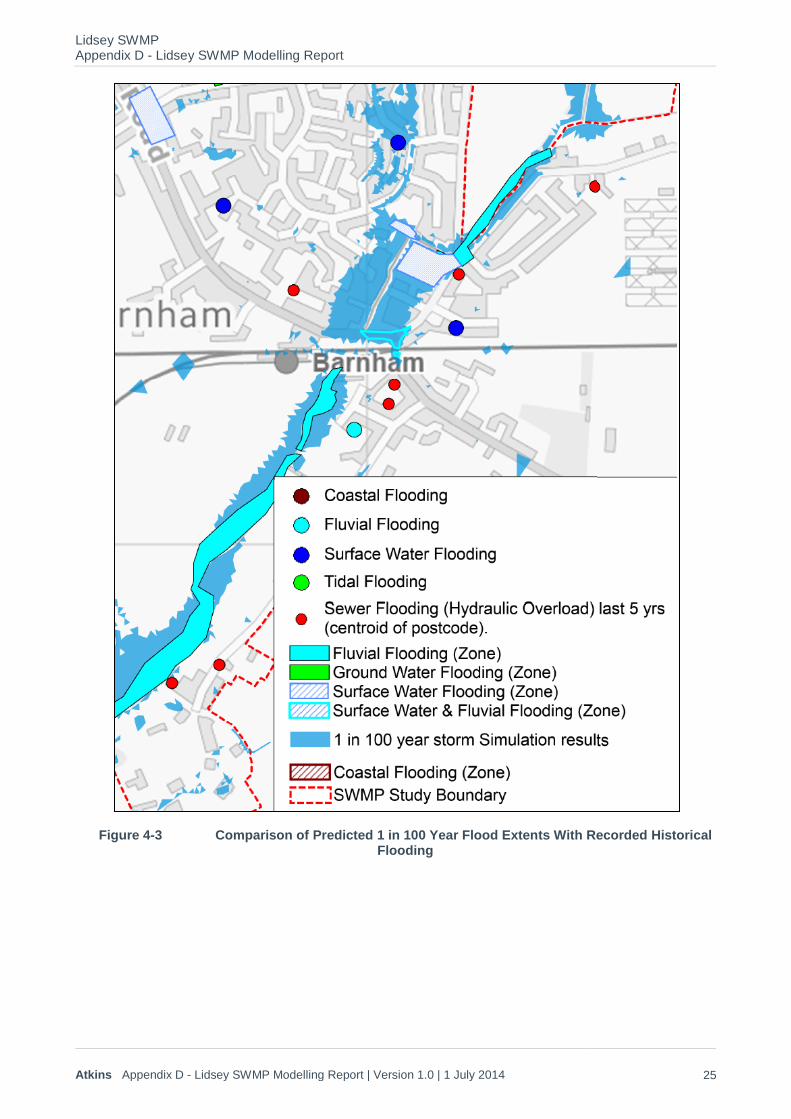
4.1.5. Design Verification A design 1 in 100 year event was simulated and compared to a dataset of recorded historical flood events across the catchment. This showed a relatively good replication of flooding issues around the study area, but also some areas where the model was not predicting flooding (refer to Figure 4-3). It is recommend that this be revisited in taking forward the project and indeed model.

A 1 in 30 year design storm event was also run in order to compare model results with the Environment Agency’s flood maps for surface water. This assessment showed a good correlation with the 2010 flood maps for surface water; however, the 2014 updated flood maps for surface water appear to under predict flooding extents in many areas, as would be expected given that these maps do not account for the full set of catchment processes (sewer systems, tides, and the groundwater system). Figure 4-4 shows a comparison at Barnham town centre.

It was considered that the InfoWorks ICM model was replicating historical flooding to a satisfactory level for use in the SWMP, but should be revisited in taking forward the project and indeed model.



Figure 4-3 Comparison of Predicted 1 in 100 Year Flood Extents With Recorded Historical Flooding



Figure 4-4 Comparison of Predicted 1 in 30 Year Flood Extents with the EA’s Flood Maps for Surface Water (2010 & 2014)



5. Model Simulation 5.1. Timestep and Runtimes The modelled timestep represents how often along a time series the model calculates its hydraulic algorithms. A lower timestep means that the model has to perform more calculations which generally increases model run times, but improves stability. Increasing the timestep increases run times and the chances for instability.

The InfoWorks ICM model was simulated with a 10 second timestep. This is the maximum (best) recommended timestep for linked 1D – 2D hydraulic models and provides the best balance of simulation runtimes and error balance.

Due to the size of the InfoWorks ICM model runtimes on lower specification computer can be considerable and it is recommended that simulations are run on computers with powerful computer processing units with Graphical Processor Units (GPUs), which decrease runtimes dramatically.

5.2. Stability The InfoWorks ICM model is considered stable, with mass error balances within acceptable range of +/- 2% for return periods of 1 in 30 years, 1 in 100 years and 1 in 1000 years.



6. Conclusions and Recommendations The InfoWorks ICM model developed for the Lidsey Surface Water Management Plan (SWMP) represents an ‘intermediate’, but sophisticated, approach to identifying flood risk across the study area. The InfoWorks ICM model explicitly represents the river, sewer, groundwater, and tidal systems in a variable level of detail to identify “at risk” areas. In subsequent work, the InfoWorks ICM model should be refined with further data and information and especially if flood risk alleviation options are pursued or the basis of the model is used to inform planning decisions.

It is recommended that the InfoWorks ICM model is:

• Integrated with the Environment Agency’s fluvial network model, which is currently being constructed, as this will have verified fluvial (main river) components.

• Improved with more detailed study into soil classes across the study area, so that the representation of rural runoff is improved e.g. use of Horton 2D infiltration surfaces.

• Increased with groundwater level survey across the catchment, as this can be used to further develop / refine the groundwater model included within the InfoWorks ICM model or be used to develop more refined and linked groundwater models.

• Increased in detail and verification in critical areas to facilitate detailed design for flood alleviation options – in particular, spatial and time series rainfall inputs should be made use of

• Improved with survey of critical drainage assets. • Used in more detailed LFRZ flood investigations, so long as refinements are included. • Considered as a basis for implementing real time control solutions / warning e.g. optimising the

wastewater treatment works and operation of overflows (including consenting). • Used to support future FDGIA funding applications.

7. References CIRIA. (2007). The SUDS manual. London: CIRIA.

DEFRA. (2005). Making Space for Water. London: DEFRA.

Pitt, M. (2008). Learning lessongs from the 2007 floods - The Pitt Review. London: DEFRA.

UK Government. (2004). Foresight Future Flooding. London: UK Government.

© Atkins Ltd except where stated otherwise. The Atkins logo, ‘Carbon Critical Design’ and the strapline ‘Plan Design Enable’ are trademarks of Atkins Ltd.

Matt McDonald Atkins Woodcote Grove Ashley Road Epsom Surrey KT18 5BW Email [email protected] Direct telephone 01372 754311

Lidsey SWMP Modelling reports

Documents

Transcript of Lidsey SWMP Modelling reports