Length and Time scale issues in Molecular

simulation

Prabal K Maiti

Center for Condensed Matter Theory, Department of

Physics

http://www.physics.iisc.ernet.in/~maiti

Ref:

Computer simulation of Liquids: M. P. Allen and D. J.

Tildesley, Oxford (1987)

Understanding Molecular simulation: Daan Frenkel and B

Smit (2nd ed)

Molecular Modelling Principles And Applications: Andrew

Leach, Prentice Hall (2001)

The art of Molecular dynamics: D. C.Rappaport

Molecular Modeling and Simulation: Tamar Schlick

What size is too big? What times are too long?

• QM (ab initio molecular dynamics)

electrons / N basis sets, speed ~ N3 or N4 (may be linear with very high prefactor)

Time steps ~10-2 fs.

Example of big and long: 64 water molecules during 10 ps.

• Classical atomistic MDAtoms/ N atoms, speed ~N2 (may be reduced with efficient algorithms, periodic coulomb is

most expensive)

Time steps ~0.5-2 fs.

Example of big and long (1 processor): 50,000 atoms for 1 ns.

(parallel simulations, can improve this much. Parallel codes available free or almost free: LAMMPS, AMBER, GROMACS, NAMD)

Short history of Molecular Simulations

• Metropolis, Rosenbluth, Teller (1953) Monte Carlo

Simulation of hard disks.

• Fermi, Pasta Ulam (1954) experiment on ergodicity

• Alder & Wainwright (1958) liquid-solid transition in hard

spheres. “long time tails” (1970)

• Vineyard (1960) Radiation damage using MD

• Rahman (1964) liquid argon, water(1971)

• Verlet (1967) Correlation functions, ...

• Andersen, Rahman, Parrinello (1980) constant pressure

MD

• Nose, Hoover, (1983) constant temperature thermostats.

• Car, Parrinello (1985) ab initio MD.

The examples for each period are

representative. The first five

systems are modeled in vacuum

and the others in solvent.

The 38 µµµµs ββββ-hairpin simulation

in 2001 represents an ensemble

(or aggregate dynamics)

simulation, as accumulated over

several short runs, rather than a

long simulation.

The table is taken from the book

by Tamar Schlick

NSF Peta scale machine

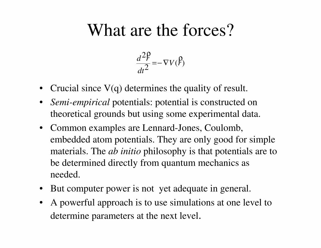
What are the forces?

• Crucial since V(q) determines the quality of result.

• Semi-empirical potentials: potential is constructed on

theoretical grounds but using some experimental data.

• Common examples are Lennard-Jones, Coulomb,

embedded atom potentials. They are only good for simple

materials. The ab initio philosophy is that potentials are to

be determined directly from quantum mechanics as

needed.

• But computer power is not yet adequate in general.

• A powerful approach is to use simulations at one level to

determine parameters at the next level.

)(2

2rV

dt

rd ρρ

∇−=

Calculation of Forces• Force is the gradient of the potential

2 1 12

12 12

1 1

12 12 12

12 1 1

1212 12

12

( )

( ) ( )

( )

( )

x y

x y

x y

u r

u r u r

x y

du r r r

dr x y

f rx y

r

→ = −∇

∂ ∂= − −

∂ ∂

∂ ∂= − + ∂ ∂

= − +

F

e e

e e

e e

2

1

r12

x12

y12

4

2

0

-2

2.52.01.51.0

Separation, r/σ

Energy Force

1/ 22 2

12 2 1 2 1( ) ( )r x x y y = − + −

Force on 1,

due to 2

2 1 1 2→ →= −F F

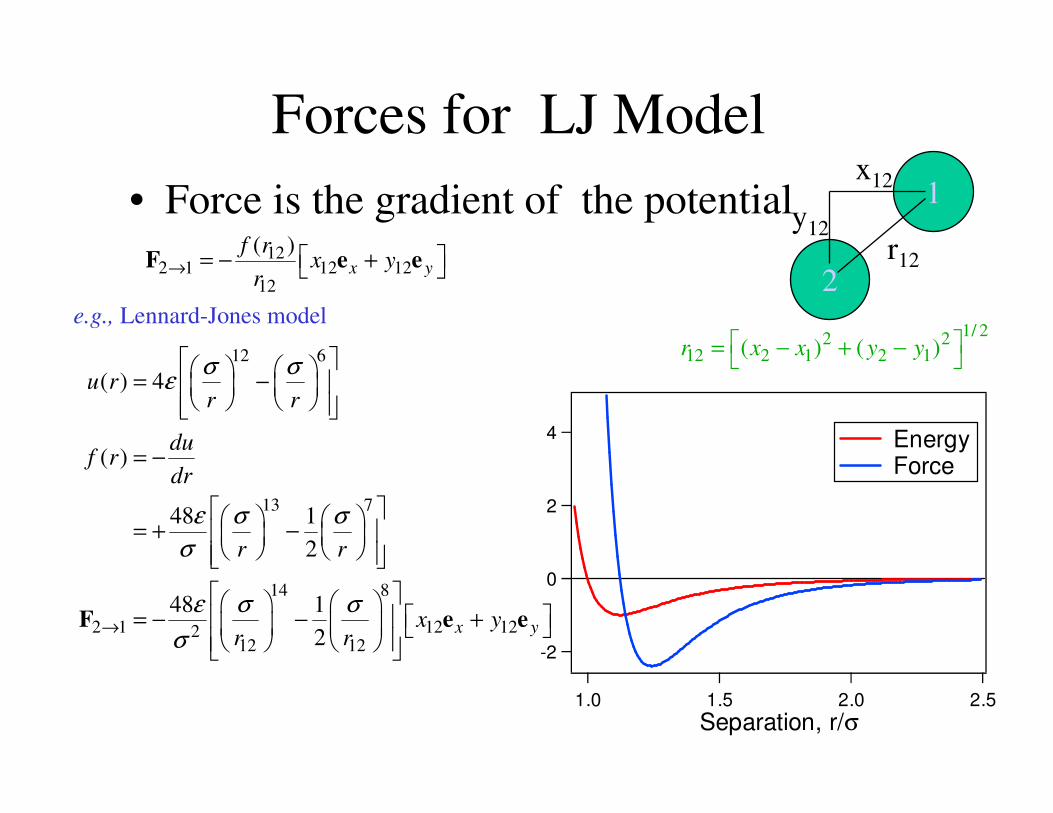
Forces for LJ Model

• Force is the gradient of the potential12

2 1 12 1212

( )x y

f rx y

r→ = − + F e e

2

1

r12

x12

y12

4

2

0

-2

2.52.01.51.0

Separation, r/σ

Energy Force

1/ 22 2

12 2 1 2 1( ) ( )r x x y y = − + −

e.g., Lennard-Jones model

12 6

13 7

14 8

2 1 12 12212 12

( ) 4

( )

48 1

2

48 1

2x y

u rr r

duf r

dr

r r

x yr r

σ σε

ε σ σ

σ

ε σ σ

σ→

= −

= −

= + −

= − − +

F e e

Dealing length scale: Boundary Conditions

• Small system is simulated to study/mimic the bulk properties

• Surface effect: a large fraction of the small sample lie on the surface. For example for 1000 molecules arranged in 10x10x10 cube, almost 400 molecules appear on the cube faces. Surface molecules/atoms experience different force than in the bulk.

• Impractical to contain system with a real boundary

– Enhances finite-size effects

– Artificial influence of boundary on system properties

Solution: Periodic boundary condition

•The problem of surface effect can be overcome by using. “Periodic Boundary Conditions” (PBC). The bounding box is replicated throughout space to form an infinite lattice. In the course of simulation as a molecule moves in the original box, its periodic images in the each of the neighboring boxes

•As the molecule leaves the central box, one of its image will enter through the opposite face.

•No physical wall at the boundary and so no surface molecules.

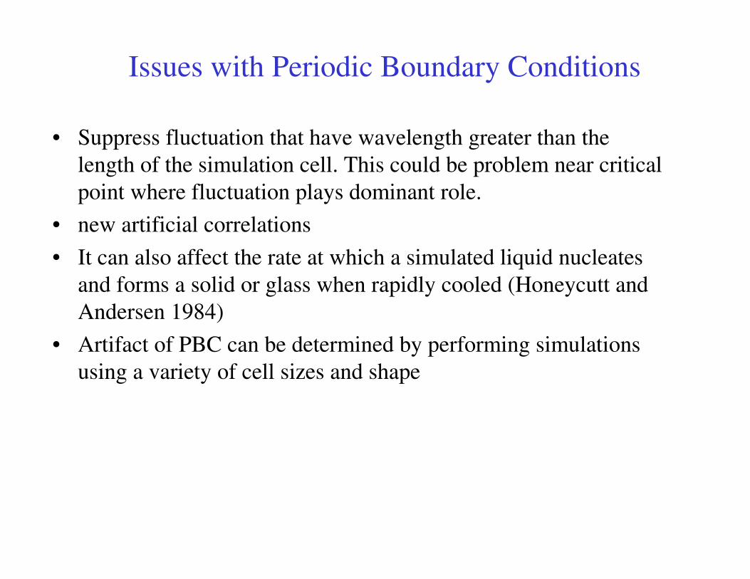
Issues with Periodic Boundary Conditions

• Suppress fluctuation that have wavelength greater than the

length of the simulation cell. This could be problem near critical

point where fluctuation plays dominant role.

• new artificial correlations

• It can also affect the rate at which a simulated liquid nucleates

and forms a solid or glass when rapidly cooled (Honeycutt and

Andersen 1984)

• Artifact of PBC can be determined by performing simulations

using a variety of cell sizes and shape

Issues with Periodic Boundary Conditions

• Other issues arise when dealing with longer-range potentials

– accounting for long-range interactions

– nearest image not always most energetic

– splitting of molecules (charges)

– discuss details later

• Other geometries possible

– any space-filling unit cell

• hexagonal in 2D

• truncated octahedron in 3D

• rhombic dodecahedron in 3D

– surface of a (hyper)sphere

– variable aspect ratio useful for solids

• relieves artificial stresses

Implementing Cubic Periodic Boundaries

• How do we handle PBC and the minimum image convention

– Box origin

• center of box, coordinates range from -L/2 to +L/2. When a molecule

leaves a box crossing one of the boundary, its image enters the box and is

accomplished either by adding or subtracting L to the particle coordinate.

If (drx[I] > L/2) rx[I] = rx[I] – L

If (drx[I] > -L/2) rx[I] = rx[I] +L

A more convenient way to handle PBC as well as

minimum image convention is to use reduce

(scaled coordinates) in the range (-1/2,1/2)

– Box size

• unit box, coordinates scaled by box length

• sep[0] = sep[0] – NINT(sep[0])

• define NINT(x) ((x) < 0.0 ? (int) ((x) - 0.5) : (int) ((x)

+ 0.5))

-0.5 +0.5+0.5

-0.5

(0,0)

Implementing Cubic Periodic Boundaries 3

void periodic_boundary_conditions(int n_atoms, double **h,

double **scaled_atom_coords, double **atom_coords)

int i, j;

for (i = 0; i < n_atoms; ++i)

for (j = 0; j < NDIM; ++j)

scaled_atom_coords[i][j] -= NINT(scaled_atom_coords[i][j]);

atom_coords[i][0] = h[0][0] * scaled_atom_coords[i][0]

+ h[0][1] * scaled_atom_coords[i][1]

+ h[0][2] * scaled_atom_coords[i][2];

atom_coords[i][1] = h[1][1] * scaled_atom_coords[i][1]

+ h[1][2] * scaled_atom_coords[i][2];

atom_coords[i][2] = h[2][2] * scaled_atom_coords[i][2];

Implementing Cubic Periodic Boundaries

void scaled_atomic_coords(int n_atoms, double **h_inv, double **atom_coords,

double **scaled_atom_coords)

int i;

for (i = 0; i < n_atoms; ++i)

scaled_atom_coords[i][0] = h_inv[0][0] * atom_coords[i][0]

+ h_inv[0][1] * atom_coords[i][1]

+ h_inv[0][2] * atom_coords[i][2];

scaled_atom_coords[i][1] = h_inv[1][1] * atom_coords[i][1]

+ h_inv[1][2] * atom_coords[i][2];

scaled_atom_coords[i][2] = h_inv[2][2] * atom_coords[i][2];

Truncating the Potential

• For system with pair wise additive interactions force on a particle I

is computed by all its neighbors. This means for a system of N

particles we have to evaluate N(N-1)/2 pair interactions. So the time

needed for evaluation of energy/force scales as N2. This is one of the

main bottleneck in the simulation field.

• Bulk system modeled via periodic boundary condition

– not feasible to include interactions with all images

– must truncate potential at half the box length (at most) to have all

separations treated consistently

• Contributions from distant separations may be important

Minimum image convention and Truncating the Potential

These two are same

distance from central

atom, yet:

Black atom interacts

Blue atom does not

How do we evaluate force on the red atom in

the simulation box. Assuming pair wise

interaction we should include interaction of

the red atom with all other atoms in the

simulation box. There are N-1 such term.

However, we must also include interaction

coming from images lying in the surrounding

boxes. That is an infinite number of terms.

Minimum image convention

Construct a simulation box of same size as

the the original box with the red atom at its

center. Now minimum image convention

says that the red atom interact with those

atoms which lie in this region, that is with

the closest periodic images of the other N-1

atoms.

Truncating the Potential

Only interactions

considered

With the minimum image convention energy/force

computation involves 1/2N(N-1) terms.This is

significant for large system size.

For short range interaction major contribution

comes from the neighbors close to the atom of

interest. So use a spherical cutoff to truncate the

interaction.

So the red atom interact only with the atoms lying

inside the cutoff region (2 black and one blue)

The cutoff distance should be smaller than L/2 to be consistent with the minimum

image convention

Thermodynamic properties are different for a truncated potential compared to a non-

truncated case. However, we can apply long range correction to get back

approximately the non-truncated properties.

Cutoff introduces discontinuity in the force and energy computation. This has

serious consequences on the energy conservation and stability of the simulation

Points to remember

Truncating the Potential contd

Potential truncation introduces discontinuity

– Corresponds to an infinite force

– Problematic for MD simulations

• ruins energy conservation

• Shifted potentials: a constant term is subtracted from the potential at all values

– Removes infinite force

– Still discontinuity in force: at the cutoff distance, the force will have a finite value which drops to zero just beyond the cutoff

( ) ( )( )

0

c cs

c

u r u r r ru r

r r

− ≤=

>

Truncating the Potential

Shifted-force potentials : a linear term can be added to the potential, making the derivative to be zero at the cutoff

– The discontinuity now appears in the gradient, not in the force itself. The force goes smoothly to zero at cutoff.

– The shift makes the potential deviate from the true potential, so the calculated thermodynamic properties will be changed

– True values can be retrieved but is difficult to do so, so rarely used in simulation

Eliminate discontinuities in the energy and force by a switching function

( ) ( ) ( )( )

0

c c csf

c

duu r u r r r r r

u r dr

r r

− − − ≤

= >

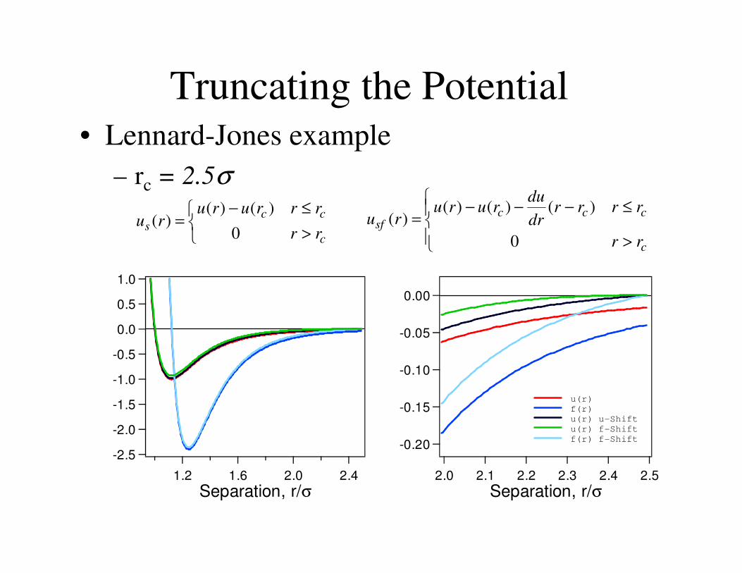
Truncating the Potential

( ) ( )( )

0

c cs

c

u r u r r ru r

r r

− ≤=

>

( ) ( ) ( )( )

0

c c csf

c

duu r u r r r r r

u r dr

r r

− − − ≤

= >

• Lennard-Jones example

– rc = 2.5σ

-2.5

-2.0

-1.5

-1.0

-0.5

0.0

0.5

1.0

2.42.01.61.2

Separation, r/σ

-0.20

-0.15

-0.10

-0.05

0.00

2.52.42.32.22.12.0

Separation, r/σ

u(r)

f(r)

u(r) u-Shift

u(r) f-Shift

f(r) f-Shift

Potential function is multiplied by a polynomial which is a function of

distance

Switching function

)()()( rSrursu =

S(r) gradually taper the potential between two cutoff values : it smoothly

changes its value of 1 to a value of 0 between two cutoff : rl (lower

cutoff) and ru (upper cutoff) and satisfies the following criteria

02

200.1

02

200.1

=

=

==

==

=

=

==

==

urrdr

Sd

urrdr

dS

urrS

lrrdr

Sd

lrrdr

dS

lrrS

Zero first derivative ensures that the force approaches to zero smoothly

at the cutoffs. A continuous second derivative ensures the stability of the

integration algorithm.

Switching function contd.

0)(

1)(

=

=

urSl

rS

3)22(2

2)22(1

)22(0

22)]22(2

3[

3

2)22()(

rurcrurcrurc

lrurwhererurrurrS

−+−+−=

−=−−−= γγ

γ

/* Calculate pair interaction. The LJ pair potential is switched off smoothly between r_on and

r_off. */

one_over_r2_sep = 1.0 / r2_sep;

rho_2 = comb_par[id_0][id_1][2] * one_over_r2_sep;

rho_6 = CUBE(rho_2);

rho_12 = SQR(rho_6);

*u_vdw = rho_12 - rho_6;

*f_vdw = rho_12 + *u_vdw;

four_epsilon = comb_par[id_0][id_1][3];

(*u_vdw) *= four_epsilon;

(*f_vdw) *= 6.0 * one_over_r2_sep * four_epsilon;

if (r2_sep > r2_on)

sw1 = r2_off - r2_sep;

sw2 = two_over_gamma_cubed * sw1;

sw3 = sw1 * sw2 * (three_gamma_over_two - sw1);

sw4 = 6.0 * sw2 * (gamma - sw1);

*f_vdw = sw4 * (*u_vdw) + sw3 * (*f_vdw);

(*u_vdw) *= sw3;

Switching function contd.

We can use higher order polynomial also

5

5

4

4

3

3

2

210)(

−

−+

−

−+

−

−+

−

−+

−

−+=

lrur

lrr

c

lrur

lrr

c

lrur

lrr

c

lrur

lrr

c

lrur

lrr

ccrS

With the coefficients satisfying the previous criteria and that gives

C0=1, c1=0, c2=0, c3=-10, c4=15, c5=-6

Verlet List

i

rl ru

Particles outside cutoff do not

contribute to the energy of the

particle I.

Exclude those particles from the

energy computation

Verlet List: Introduce a second

cutoff radius ru >rl

Make a list of all the particles

within a radius of ru of particle i

If the maximum displacement of

the particles is less than (ru -rl) we

have to consider only the particles

in this list for the energy/force

computation

Update the Verlet list as soon as

one of the particle is displaced

more than (ru -rl)

For MD it is sufficient to have a Verlet list with half the number of

particles for each particle as long as interaction i-j is accounted for in

either the list of particle i or that of j

1

2

34

5

6

7

rc

7’

ru

The cutoff sphere and its skin around

an atom 1. Atoms 2,3,4,5 and 6 are on

the list of atom 1, but 7 is not. Among

these only 2,3,4 are within the rc when

the list is made

The skin is thick enough such that

when reconstructing an atom 7,

which was not in the original list of

atom 1can not penetrate the rc sphere.

Atom 3, 4 can move in and out but

their interaction get counted as they

are in the original list until the list get

updated.

From Allen and Tildesley

For a periodic system Verlet list has an elegant implementation due to

Bekker et. al. (Mol. Sim. 14, 137-151, 1995)

)(1

13

13

/

jkiF

N

j ki

F ∑=

∑−=

=

In a periodic system total force on particle i can be written as

Where the prime denotes that summation is performed over the nearest

image of the particle j in the central box (k=0) or in one of its 26

periodic images (or 8 in 2-d). (j.k) denotes the periodic image of

particle j in box k. Box k is defined by the integer numbers nx, ny, nz

k = 9nx+3 ny + nz

As the size of the system increases neighbor list becomes too large to

store easily

Also the testing of every pair separation is also very inefficient

Make the neighbor list using Cell list

Problem with Verlet List

Cell Lists or Linked-list

The simulation box is divided into cells with size equal to or slightly

larger than the cutoff rc

Distribute the particle to the cell according to their position

Each particle in a given cell interacts with only those particles in the

same or neighboring cells

This scales as N rc

The simulation cell is divided into

cells of size rc x rc, a particle i

interacts with those particles in the

same cell or neighboring cell (in 2D

9 cells; in 3D 27 cells)

i

The Cell list is created using the linked list methods:

Sorting of atoms to their respective cells

Two arrays are created (HEAD AND LIST)

HEAD (head of the chain) array has one element for each cell. This

contains the identification number of one of the molecules sorted into

that cell

LIST (linked list array) contains the number of next molecules in

that cell.

HEAD (head of the chain) array element is used to address the LIST

array element.

If we follow the trail of linked-list we will eventually reach an

element of LIST which is zero. This indicates that there are no more

molecules in that cell and we move on to the head of chain of the next

cell.

See Allen and Tildesley for details

void neighbor_lists_period()

/* Purge neighbor lists. */

for (i = 0; i < n_atoms; ++i)

nl_tail[i] = NULL;

/* Update cell lists. */

update_cells(period_switch, n_atoms, h, scaled_atom_coords, atom_coords,

atom_cells, first, last, phantoms, kc, phantom_skip, nc, nc_p);

/* Update positions of phantom atoms. */

update_phantoms(n_atoms, atom_cells, phantom_skip, phantoms, atom_coords);

/* Loop over central atoms. */

for (i = 0; i < n_atoms; ++i)

/* Get attributes of atom i. */

for (k = 0; k < NDIM; ++k)

Radial Distribution Function

• Radial distribution function, g(r)

– key quantity in statistical mechanics

– quantifies correlation between atom pairs

• Definition

( )( )

( )id

r dg r

r d

ρ

ρ=

r

r

Number of atoms at

r for ideal gas

Number of atoms at

r in actual system

( )id Nr d d

Vρ =r r

dr

4

3

2

1

0

543210

Hard-sphere g(r) Low density High density

),(),(2

1),(

jr

ira

jr

irg

jdr

idr

Vj

ri

ra ∫=

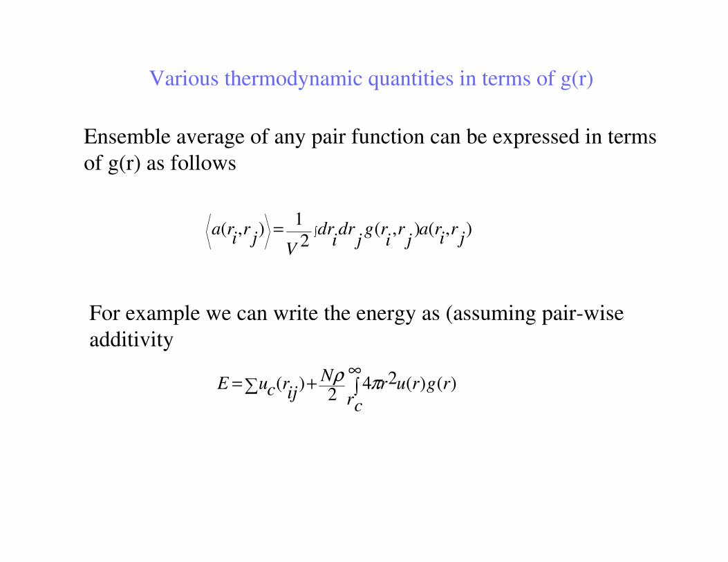
Various thermodynamic quantities in terms of g(r)

Ensemble average of any pair function can be expressed in terms

of g(r) as follows

For example we can write the energy as (assuming pair-wise

additivity

)()(242

)( rgru

crrN

ijrcuE ∫

∞+∑= πρ

Simple Long-Range Correction

• Approximate distant interactions by assuming

uniform distribution beyond cutoff: g(r) = 1 r > rcut

• Corrections to thermodynamic properties

– Internal energy

– Virial

– Chemical potential

2( )42

cut

lrc

r

NU u r r drρ π

∞

= ∫Expression for Lennard-Jones model

2 214

6cut

lrc

r

duP r r dr

drρ π

∞

= ∫

2( )4 2

cut

lrclrc

r

Uu r r dr

Nµ ρ π

∞

= =∫

9 3

383

9

LJlrc

c c

U Nr r

σ σπ ρσ ε

= −

9 3

2 332 3

9 2

LJlrc

c c

Pr r

σ σπρ σ ε

= −

For rc/σ = 2.5, these are about

5-10% of the total values

Overcoming time issues

• Ewlad method O(N3/2)

• Particle Mesh Ewald O(NlogN)

• Cell Multipole Methods O(N)

• Newton’s equation of motion are time reversible and so should be

our algorithm.

• Hamiltonian dynamics preserve the magnitude of volume element in

phase space and so our algorithm should have this area preserving

property

• simplicity (How long does it take to write and debug?)

• efficiency (How fast to advance a given system?)

• stability (what is the long-term energy conservation?)

• reliability (Can it handle a variety of temperatures, densities,

potentials?)

Criteria for an Integrator

The nearly universal choice for an integrator is the Verlet (leapfrog) algorithm

r(t+δt) = r(t) + v(t) δt + 1/2 a(t) δt 2 + b(t) δt 3 + O(δt 4) Taylor expand

r(t- δt) = r(t) - v(t) δt + 1/2 a(t) δt 2 - b(t) δt 3 + O(δt 4) Reverse time

r(t+ δt) = 2 r(t) - r(t- δt) + a(t) δt 2 + O(δt 4) Add

v(t) = (r(t+ δt) - r(t- δt))/(2 δt) + O(δt 2) estimate velocities

Time reversal invariance is built in the energy does not drift.

Velocity is not required to compute the new position.

Once the new position is computed using position at t- δt, discard the old

Position. The current position become the old positions and the new position

become the current position.

Note that velocity is used only to compute the kinetic energy and hence the

temperature of the system

Time reversible and area preserving

Tuckerman, Berne, Martyna, JCP, 97, 1990 1992

Linear Stability analysis for Harmonic oscillator

xxF 2)( ω−=

=

+

+

)(

)(

)(

)(

tv

txS

ttv

ttx ω

δ

δω

−−

−−=

2/1

)4/1(2/1

2

22

εε

εεεS

Position Verlet scheme can be written as

where tωδε =and

42 <ε

πωδ

2//2

pTt<< ωπ /2=pT

Powers of S is bonded if

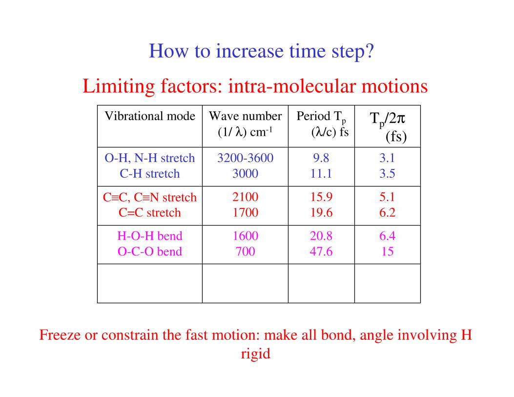
How to increase time step?

Limiting factors: intra-molecular motions

6.4

15

5.1

6.2

3.1

3.5

Tp/2π(fs)

1600

700

2100

1700

3200-3600

3000

Wave number

(1/ λ) cm-1

20.8

47.6

H-O-H bend

O-C-O bend

15.9

19.6

C≡C, C≡N stretch

C=C stretch

9.8

11.1

O-H, N-H stretch

C-H stretch

Period Tp

(λ/c) fs

Vibrational mode

Freeze or constrain the fast motion: make all bond, angle involving H

rigid

How to increase time step?

Multiple time steps algorithm

Short-range interactions governs the intra-molecular motion, time scale

of which are very fast. In that time scale “long range” part of the

interaction hardly changes and need not be computed at same frequency

of the short range interactions.

longshort FFF +=

longmedshort FFFF ++=

or

a time step to compute short-range interactions

another time stop to compute medium range interactions

another time step to compute long-range interactions

Use Multiple time steps

Solvation Models

in Molecular Simulations

•Explicit Solvent

Large system - CPU intensive

Long equilibration simulation times

Quality depends on forcefield used

•Implicit Solvent

Continuous: medium surrounding solute

SASA: Solvent Accessible solute interaction

GB:Treat long-range effects

AVGB: add short-range effects to GB

Water Solvation Effects

•Long Range Effects (Electrostatic)

Solute Polarization (reaction field)

Dielectric Screening

•Short Range Effects (contraction to 1st solvation shell)

Dispersion Interactions (vdW)Cavity Formation (Entropic)

Hydrogen Bonding (Charge Transfer)

The solvation free energy is the free energy change to transfer a molecule from vacuum

to solvent. The solvation free energy has three components

cavGvdw

Gelec

Gsolv

G ∆+∆+∆=∆

elecG∆ is the electrostatic component: very important component for polar and

charged solute

is the van der Walls interaction between the solute and solventvdwG∆

cavG∆ is the free energy required to form the solute cavity within the solvent. This

component is positive and comprises the entropic penalty associated with the

reorganization of the solvent molecules around the solute together with the

work done against the solvent pressure to create the cavity

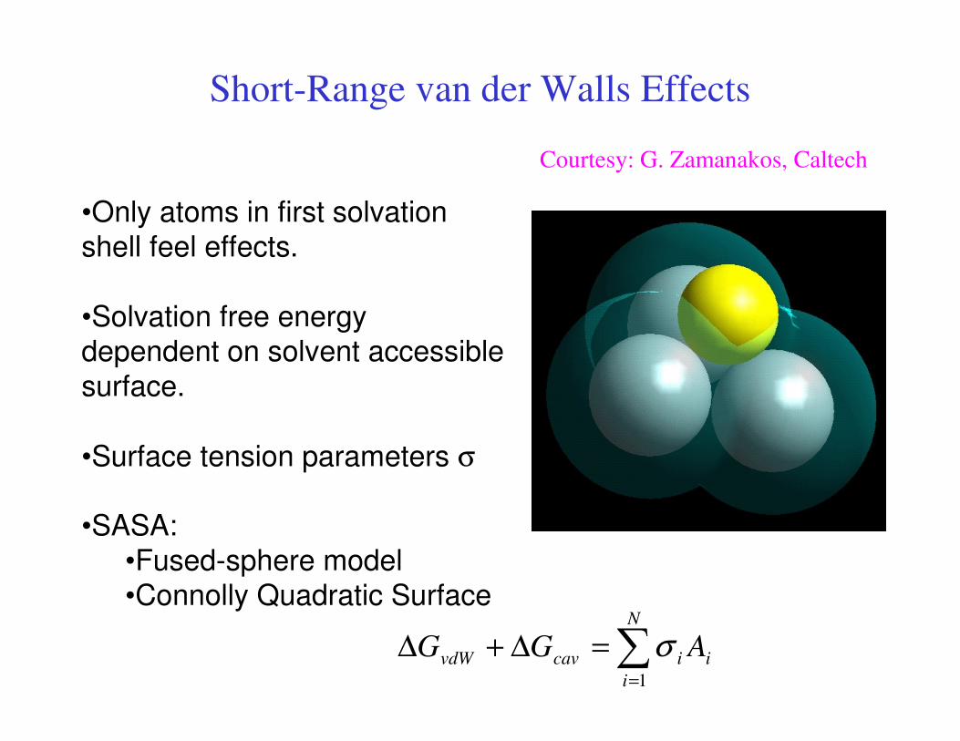
Short-Range van der Walls Effects

•Only atoms in first solvation shell feel effects.

•Solvation free energy dependent on solvent accessible

surface.

•Surface tension parameters σ

•SASA:

•Fused-sphere model•Connolly Quadratic Surface

∑=

=∆+∆N

i

iicavvdW AGG1

σ

Courtesy: G. Zamanakos, Caltech

Long Range Effects

Continuum Dielectric Approximation: Poisson-Boltzman

)(4)()( rrrρρρ

πρε =Φ∇⋅∇−

)(rρ

Φ Electrostatic potential dielectric, screening, and charge density)(),(),( rrrρρρ

ρκε

The solute is treated as a body of constant low dielectric and the solvent is modeled as a

continuum of high dielectric

επρφ )(4

)(2 rr −=∇

For a set of point charges in a constant dielectric medium the Poisson equation

reduces to Coulomb’s Law

When dielectric changes with position Poisson equation becomes

)(4)(sinh2)()()( rrrrrρρρρρ

πρκε =Φ+Φ∇⋅∇−

)(rρ

κ

When mobile ions are present Poisson equation needs to be modified to take into

account for their redistribution in the solution in response to the electric potential. The

ions distribution is described by a Boltzmann distribution of the form

)/)(exp()( TB

krVNrn −= n(r) is the number density at position r

N is the bulk number density

V(r) is the energy change to bring the ion from

infinity to the position r

When the above fact is taken into consideration the Poisson equation becomes Poisson-

Boltzmann equation

is related to the inverse of the Debye-Huckel length

Expanding the hyperbolic sine function as Taylor series and keeping only the first term we

have linearised Poisson-Boltamann equation

)(4)(2)()()( rrrrrρρρρρ

πρκε =Φ+Φ∇⋅∇−

•Numerical solution, CPU intensive, scales as )( 3NO

•Lack of gradients (atomic forces) •Accuracy depends on grid resolution.

•Applications show successful predictions.

•Not parallelizable, QM implementations available

The Generalized Born Model

•Polar Solvation Energy of a charged sphere of radius R and

permittivity εin in dielectric medium εout (Born):

R

qG

outin

pol

211

2

1

−−=∆

εε

•System of N spheres of radii αi, far away from each other:

+

−−=∆ ∑∑∑

=≠ ==

N

ji

N

j ij

jiN

i i

i

outin

polr

qqqG

1 11

211

2

1

αεε

•We seek interpolation formula between the two limits:

∑∑= =

−−=∆

N

i

N

j ij

ji

outin

polf

qqG

1 1

11

2

1

εε

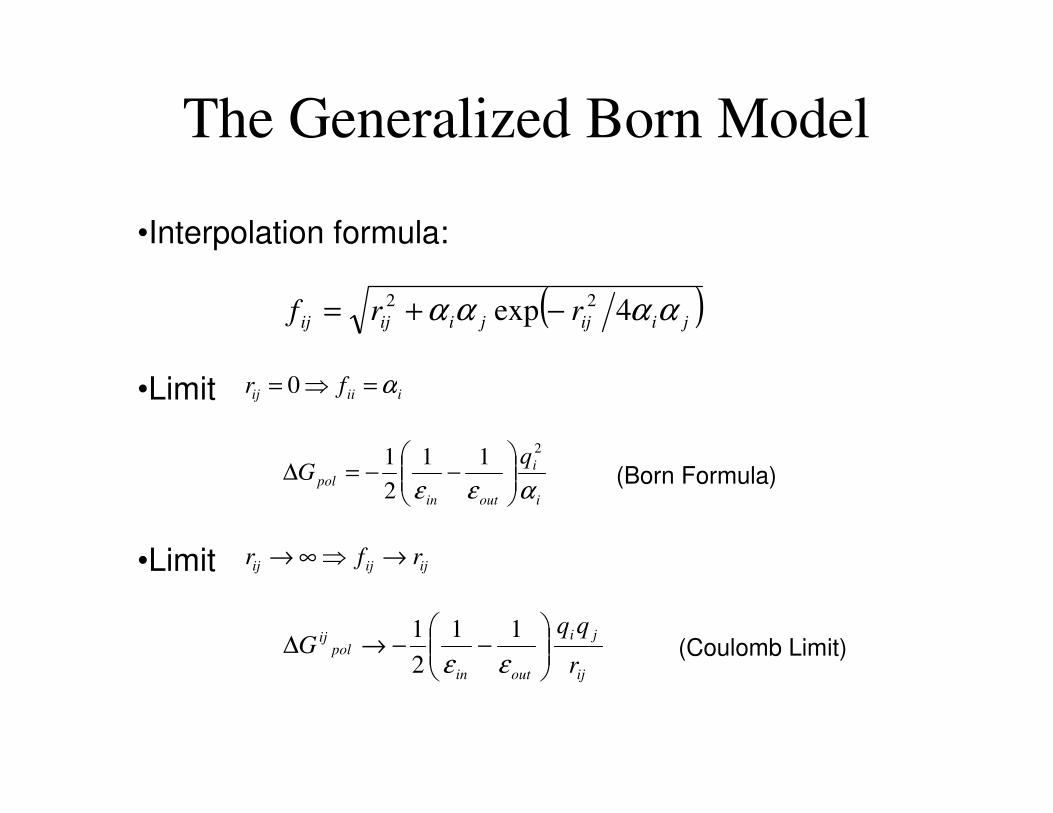
The Generalized Born Model

( )jiijjiijij rrf αααα 4exp 22 −+=

•Interpolation formula:

•Limit iiiij fr α=⇒= 0

i

i

outin

pol

qG

αεε

211

2

1

−−=∆ (Born Formula)

•Limit ijijij rfr →⇒∞→

ij

ji

outin

polij

r

qqG

−−→∆

εε

11

2

1(Coulomb Limit)

Born Radii

•If we set all charges to zero except qk, we get:

k

k

outin

pol

qG

αεε

211

2

1

−−=∆

•Parameters αk are the Born Radii.

•Physical Meaning: the effective radius of an ion of charge qk, whose solvation energy is equal to the

self-energy of polarization of atom in the molecule.

•Difficult to calculate.

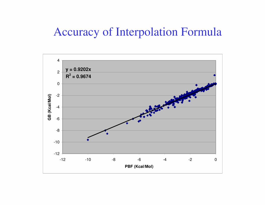
Accuracy of Interpolation Formula

y = 0.9202x

R2 = 0.9674

-12

-10

-8

-6

-4

-2

0

2

4

-12 -10 -8 -6 -4 -2 0

PBF (Kcal/Mol)

GB

(K

ca

l/M

ol)

Calculation of Born Radii

•Solute charge distribution polarizes solvent which in turn interacts with the solute (reaction field ).)(rreac

ρΦ

•Assume the reaction field is coulombic in nature. It can be proven that:

∫Ω −

−=

k

rdrrR

kkk

3

4

1

4

111ρρπα

•Pairwise approximation:

∑ ∫∫≠Ω −

=− kk V kk kk

rdrr

rdrr '

3

4

3

4

'

11ρρρρ

•Analytical solution exists for integral over sphere Need volumes of every atom.

3

4

3

πkeff

k

VR =

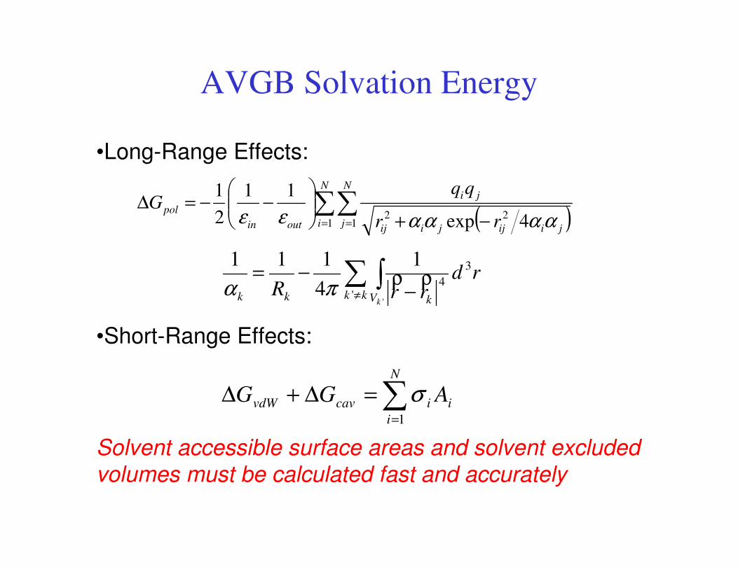
AVGB Solvation Energy

•Long-Range Effects:

( )∑∑= = −+

−−=∆

N

i

N

jjiijjiij

ji

outin

pol

rr

qqG

1 122 4exp

11

2

1

ααααεε

∑ ∫≠ −

−=kk V kkk

k

rdrrR '

3

4

'

1

4

111ρρπα

•Short-Range Effects:

∑=

=∆+∆N

i

iicavvdW AGG1

σ

Solvent accessible surface areas and solvent excluded volumes must be calculated fast and accurately

The Fused-Sphere Model

•Analytical calculation of volumes and areas, with

gradients

•Complicated topologies

•Robust algorithms

Area Calculation

Gauss-Bonnet Theorem

( ) ( ) ( )∑∑ ∫∫∫==

=Ω++m

i

i

n

i RC

g RdssKdllk

i11

2πχ

Geodesic curvature, gaussian curvature of surface, Euler-Poincare characteristic of surface R

External angles of surface

Zamanakos, Phd thesis (Caltech), 2002