New Finite Element Models and Seismic Analyses of the Telescopes at W.M. Keck Observatory

KECK GEOLOGY CONSORTIUM
PROCEEDINGS OF THE TWENTY-FOURTH ANNUAL KECK RESEARCH SYMPOSIUM IN
GEOLOGY
April 2011 Union College, Schenectady, NY
Dr. Robert J. Varga, Editor Director, Keck Geology Consortium
Pomona College
Dr. Holli Frey
Symposium Convenor Union College
Carol Morgan Keck Geology Consortium Administrative Assistant
Diane Kadyk Symposium Proceedings Layout & Design
Department of Earth & Environment Franklin & Marshall College
Keck Geology Consortium Geology Department, Pomona College
185 E. 6th St., Claremont, CA 91711 (909) 607-0651, [email protected], keckgeology.org
ISSN# 1528-7491
The Consortium Colleges The National Science Foundation ExxonMobil Corporation

KECK GEOLOGY CONSORTIUM PROCEEDINGS OF THE TWENTY-FOURTH ANNUAL KECK
RESEARCH SYMPOSIUM IN GEOLOGY ISSN# 1528-7491
April 2011
Robert J. Varga
Editor and Keck Director Pomona College
Keck Geology Consortium Pomona College
185 E 6th St., Claremont, CA 91711
Diane Kadyk Proceedings Layout & Design Franklin & Marshall College
Keck Geology Consortium Member Institutions:
Amherst College, Beloit College, Carleton College, Colgate University, The College of Wooster, The Colorado College, Franklin & Marshall College, Macalester College, Mt Holyoke College,
Oberlin College, Pomona College, Smith College, Trinity University, Union College, Washington & Lee University, Wesleyan University, Whitman College, Williams College
2010-2011 PROJECTS
FORMATION OF BASEMENT-INVOLVED FORELAND ARCHES: INTEGRATED STRUCTURAL AND SEISMOLOGICAL RESEARCH IN THE BIGHORN MOUNTAINS, WYOMING Faculty: CHRISTINE SIDDOWAY, MEGAN ANDERSON, Colorado College, ERIC ERSLEV, University of Wyoming Students: MOLLY CHAMBERLIN, Texas A&M University, ELIZABETH DALLEY, Oberlin College, JOHN SPENCE HORNBUCKLE III, Washington and Lee University, BRYAN MCATEE, Lafayette College, DAVID OAKLEY, Williams College, DREW C. THAYER, Colorado College, CHAD TREXLER, Whitman College, TRIANA N. UFRET, University of Puerto Rico, BRENNAN YOUNG, Utah State University. EXPLORING THE PROTEROZOIC BIG SKY OROGENY IN SOUTHWEST MONTANA Faculty: TEKLA A. HARMS, JOHN T. CHENEY, Amherst College, JOHN BRADY, Smith College Students: JESSE DAVENPORT, College of Wooster, KRISTINA DOYLE, Amherst College, B. PARKER HAYNES, University of North Carolina - Chapel Hill, DANIELLE LERNER, Mount Holyoke College, CALEB O. LUCY, Williams College, ALIANORA WALKER, Smith College. INTERDISCIPLINARY STUDIES IN THE CRITICAL ZONE, BOULDER CREEK CATCHMENT, FRONT RANGE, COLORADO Faculty: DAVID P. DETHIER, Williams College, WILL OUIMET. University of Connecticut Students: ERIN CAMP, Amherst College, EVAN N. DETHIER, Williams College, HAYLEY CORSON-RIKERT, Wesleyan University, KEITH M. KANTACK, Williams College, ELLEN M. MALEY, Smith College, JAMES A. MCCARTHY, Williams College, COREY SHIRCLIFF, Beloit College, KATHLEEN WARRELL, Georgia Tech University, CIANNA E. WYSHNYSZKY, Amherst College. SEDIMENT DYNAMICS & ENVIRONMENTS IN THE LOWER CONNECTICUT RIVER Faculty: SUZANNE O’CONNELL, Wesleyan University Students: LYNN M. GEIGER, Wellesley College, KARA JACOBACCI, University of Massachusetts (Amherst), GABRIEL ROMERO, Pomona College. GEOMORPHIC AND PALEOENVIRONMENTAL CHANGE IN GLACIER NATIONAL PARK, MONTANA, U.S.A. Faculty: KELLY MACGREGOR, Macalester College, CATHERINE RIIHIMAKI, Drew University, AMY MYRBO, LacCore Lab, University of Minnesota, KRISTINA BRADY, LacCore Lab, University of Minnesota
Students: HANNAH BOURNE, Wesleyan University, JONATHAN GRIFFITH, Union College, JACQUELINE KUTVIRT, Macalester College, EMMA LOCATELLI, Macalester College, SARAH MATTESON, Bryn Mawr College, PERRY ODDO, Franklin and Marshall College, CLARK BRUNSON SIMCOE, Washington and Lee University. GEOLOGIC, GEOMORPHIC, AND ENVIRONMENTAL CHANGE AT THE NORTHERN TERMINATION OF THE LAKE HÖVSGÖL RIFT, MONGOLIA Faculty: KARL W. WEGMANN, North Carolina State University, TSALMAN AMGAA, Mongolian University of Science and Technology, KURT L. FRANKEL, Georgia Institute of Technology, ANDREW P. deWET, Franklin & Marshall College, AMGALAN BAYASAGALN, Mongolian University of Science and Technology. Students: BRIANA BERKOWITZ, Beloit College, DAENA CHARLES, Union College, MELLISSA CROSS, Colgate University, JOHN MICHAELS, North Carolina State University, ERDENEBAYAR TSAGAANNARAN, Mongolian University of Science and Technology, BATTOGTOH DAMDINSUREN, Mongolian University of Science and Technology, DANIEL ROTHBERG, Colorado College, ESUGEI GANBOLD, ARANZAL ERDENE, Mongolian University of Science and Technology, AFSHAN SHAIKH, Georgia Institute of Technology, KRISTIN TADDEI, Franklin and Marshall College, GABRIELLE VANCE, Whitman College, ANDREW ZUZA, Cornell University. LATE PLEISTOCENE EDIFICE FAILURE AND SECTOR COLLAPSE OF VOLCÁN BARÚ, PANAMA Faculty: THOMAS GARDNER, Trinity University, KRISTIN MORELL, Penn State University Students: SHANNON BRADY, Union College. LOGAN SCHUMACHER, Pomona College, HANNAH ZELLNER, Trinity University. KECK SIERRA: MAGMA-WALLROCK INTERACTIONS IN THE SEQUOIA REGION Faculty: JADE STAR LACKEY, Pomona College, STACI L. LOEWY, California State University-Bakersfield Students: MARY BADAME, Oberlin College, MEGAN D’ERRICO, Trinity University, STANLEY HENSLEY, California State University, Bakersfield, JULIA HOLLAND, Trinity University, JESSLYN STARNES, Denison University, JULIANNE M. WALLAN, Colgate University. EOCENE TECTONIC EVOLUTION OF THE TETONS-ABSAROKA RANGES, WYOMING Faculty: JOHN CRADDOCK, Macalester College, DAVE MALONE, Illinois State University Students: JESSE GEARY, Macalester College, KATHERINE KRAVITZ, Smith College, RAY MCGAUGHEY, Carleton College.
Funding Provided by: Keck Geology Consortium Member Institutions
The National Science Foundation Grant NSF-REU 1005122 ExxonMobil Corporation

Keck Geology Consortium: Projects 2010-2011
Short Contributions— Front Range, CO
INTERDISCIPLINARY STUDIES IN THE CRITICAL ZONE, BOULDER CREEK CATCHMENT, FRONT RANGE, COLORADO Project Faculty: DAVID P. DETHIER: Williams College, WILL OUIMET: University of Connecticut CORING A 12KYR SPHAGNUM PEAT BOG: A SEARCH FOR MERCURY AND ITS IMPLICATIONS ERIN CAMP, Amherst College Research Advisor: Anna Martini EXAMINING KNICKPOINTS IN THE BOULDER CREEK CATCHMENT, COLORADO EVAN N. DETHIER, Williams College Research Advisor: David P. Dethier THE DISTRIBUTION OF PHOSPHORUS IN ALPINE AND UPLAND SOILS OF THE BOULDER CREEK, COLORADO CATCHMENT HAYLEY CORSON-RIKERT, Wesleyan University Research Advisor: Timothy Ku RECONSTRUCTING THE PINEDALE GLACIATION, GREEN LAKES VALLEY, COLORADO KEITH M. KANTACK, Williams College Research Advisor: David P. Dethier CHARACTERIZATION OF TRACE METAL CONCENTRATIONS AND MINING LEGACY IN SOILS, BOULDER COUNTY, COLORADO ELLEN M. MALEY, Smith College Research Advisor: Amy L. Rhodes ASSESSING EOLIAN CONTRIBUTIONS TO SOILS IN THE BOULDER CREEK CATCHMENT, COLORADO JAMES A. MCCARTHY, Williams College Research Advisor: David P. Dethier USING POLLEN TO UNDERSTAND QUATERNARY PALEOENVIRONMENTS IN BETASSO GULCH, COLORADO COREY SHIRCLIFF, Beloit College Research Advisor: Carl Mendelson STREAM TERRACES IN THE CRITICAL ZONE – LOWER GORDON GULCH, COLORADO KATHLEEN WARRELL, Georgia Tech Research Advisor: Kurt Frankel METEORIC 10BE IN GORDON GULCH SOILS: IMPLICATIONS FOR HILLSLOPE PROCESSES AND DEVELOPMENT CIANNA E. WYSHNYSZKY, Amherst College Research Advisor: Will Ouimet and Peter Crowley
Keck Geology Consortium Pomona College
185 E. 6th St., Claremont, CA 91711 Keckgeology.org

INTRODUCTION
Processes in the critical zone, the life-sustaining sur-ficial mantle of the earth, involve weathered geologic materials, water, and the biosphere, mediated by atmospheric processes that are controlled by changing climate. Field and laboratory studies that investigate geologic, hydrologic and geochemical components of the critical zone provide valuable data about pro-cesses and the physical basis for their integration into models of short and long-term geomorphic, hydro-logic and biochemical response. The Keck Colo-rado Project is working in cooperation with a large interdisciplinary study of the critical zone (Boulder Creek Critical Zone Observatory: Weathered profile development in a rocky environment and its influence on watershed hydrology and biogeochemistry— Su-zanne Anderson, PI, Institute for Arctic and Alpine Studies, University of Colorado). The observatory (CZO) consists of 3 small, instrumented catchments in the Boulder Creek basin, Colorado Front Range: (1) Green Lakes Valley (GLV; el. 3400 m)--a steep, glacially scoured alpine area in the City of Boulder watershed; (2) Gordon Gulch (el. 2600 m)--a forested, mid-elevation catchment that exposes isolated bed-rock remnants (tors) developed on a surface of low relief; and (3) Betasso gulch (el. 1950 m)--a steep, thinly forested basin that preserves thick regolith in the upper catchment and exposes extensive bedrock outcrops at lower elevations (Fig. 1).
The glaciated GLV, low relief surface, and bedrock canyons are developed in granitic or gneissic rocks and are influenced by the strong gradient in elevation, climate and vegetation from west to east. Variation in critical-zone development in these different envi-ronments allows us to test models of weathering and regolith generation, elemental cycling, slope evolu-tion and sediment transport in an accessible field setting. Land-use, vegetation and hydrologic response
INTERDISCIPLINARY STUDIES IN THE CRITICAL ZONE, BOULDER CREEK CATCHMENT, FRONT RANGE, COLORADODAVID P. DETHIER, Williams CollegeWILL OUIMET, University of Connecticut
24th Annual Keck Symposium: 2011 Union College, Schenectady, NY
93
in each CZO catchment also reflect changes produced by anthropogenic activities such as mining and timber harvest over the past 150 years. Keck Colorado field studies focus on using a variety of techniques to map and characterize the geologic history, near-surface geologic materials and geochemical properties for each of the study catchments.
SETTING
The middle Boulder Creek catchment (Fig. 1) extends from the glaciated alpine zone of the Continental Divide east to the semi-arid western edge of the Great Plains. The high-relief zone of cirques and deep, U-shaped valleys in the glaciated area become shallower eastward through a zone of low relief and relatively low slopes. To the east, valleys deepen into steep, narrow bedrock canyons as they pass knickzones, and flatten to lower channel slopes near the piedmont mar-gin. Small glaciers and late-persisting snowfields dot the alpine zone, which exposes bedrock and relatively thin deposits related to the latest Pleistocene Pinedale glaciation and to Holocene erosion. The forested zone
Figure 1. Perspective view looking west across the Front Range from Boulder, Colorado, showing Middle Boulder Creek and location of Betasso, Gordon Gulch and Green Lakes Valley catchments, Boulder Creek Critical Zone Observatory. White filled area shows approximate extent of latest Pleistocene glaciers (after Madole et al., 1999).

24th Annual Keck Symposium: 2011 Union College, Schenectady, NY
94
Erin Camp (Amherst), who were supported directly by NSF funding. David Dethier and Will Ouimet supervised students on a daily basis and field teams frequently joined investigators and graduate students from the University of Colorado. Matthias Leopold (Technical University of Munich) worked with Keck students for two weeks in the field. Keck students were among the only undergraduates to present pre-liminary results of their field research at the 3rd an-nual Boulder Creek CZO meeting on 10 August 2010. Keck Colorado students worked in pairs on a daily basis and sometimes as geophysical support teams. Geophysical data provided important background data for extensive studies in Gordon Gulch and for coring of bogs (Fig. 2).
Short papers elsewhere in this volume report results of the field and laboratory studies in some detail. We summarize and provide brief comments on this research here.
Studies of trace metals in organic sediment, soil and regolith in Gordon Gulch and adjacent areas
Erin Camp (Amherst) reports “Coring a 12 kyr sphag-num bog in the N. Boulder Creek valley—a search for mercury and its implications” and Ellie Maley (Smith) worked on “Characterization of trace metal concentrations and mining legacy in soils, Boulder County, Colorado”. Both of these studies dem-onstrate that Hg is enriched in recent organic-rich
of low relief exposes local areas of thick (characteris-tically 3 to 8 m) regolith, saprolite and oxidized bed-rock, but the weathered mantle is thin in other areas. Low terraces and alluvial fans as thick as 4 m line channels locally. In the vicinity of knickzones and in downstream areas such as Betasso gulch, slopes near channels are steep and fresh bedrock is exposed, whereas areas more distant from channels retain a thicker weathered mantle.
APPROACH In our third project year, we used field mapping and sampling in all three CZO catchments, supplemented by geophysical measurements, in order to provide basic data about soils and their geochemistry, shal-low subsurface geology and erosional history of the critical zone. Students supported by the Keck Geology consortium and by NSF learned geophysi-cal techniques and initial data reduction, processing and visualization methods in these settings. Students chose from a variety of potential projects in the study catchments; 2010 project topical areas included:
1. Trace-metal studies of soils and bog sediment, Boulder Creek catchment 2. Soil chemistry (Fe and P) in CZO catchments and meteoric 10Be studies of soils, focused on Gordon Gulch3. Stratigraphy and palynology of valley-fill sediment, Gordon and Betasso catchments4. Geomorphic research: Ice erosion and geo morphic evolution of the Green Lakes Valley and the evolution of knickpoints along chan- nels in the Boulder Creek catchment
We ran resistivity lines in Gordon Gulch, resistivity and ground-penetrating radar on Niwot Ridge and ground-penetrating radar in the vicinity of the bogs near the N. Branch Boulder Creek. In Gordon Gulch, we worked on regolith studies in cooperation with investigators from the University of Colorado and the US Geological Survey.
STUDENT PROJECTS
Six Keck students joined Williams students Evan Dethier, Keith Kantack and James McCarthy and
Figure 2. Coring a bog in a late Pinedale moraine com-plex along the N. Fork Boulder Creek, supervised by Robert Nelson, Colby College.

24th Annual Keck Symposium: 2011 Union College, Schenectady, NY
95
sediment of the montane zone when compared to older bog sediment or to soil C-horizons. The bog Hg profile and 14C ages show a strong correspondence between elevated Hg levels and large, silicic volcanic eruptions in Holocene time. Peak Hg levels produced by eruptions decline over narrow intervals. Mercury concentrations in bog sediments increase to a broad peak coincident with exploitation of precious metals in the western hemisphere beginning in the 16th cen-tury and peaking in the late 19th century in Colorado. Ellie’s work shows that Hg, As and possibly Pb are enriched in organic-rich O and A-horizons compared to soil parent material; other minor elements such as Cu and Zn do not show enrichment. Ellie’s research suggests that metal enrichment likely represents the legacy of local metal mining, milling and smelting, and the affinity of organic matter for these relatively volatile trace metals.
Studies of soil and regolith geochemistry and age in Gordon Gulch and adjacent areas
Four students, including Ellie Maley, studied soils and regolith exposed in pits that were dug in Gor-don Gulch and at other nearby exposures. The “pit crew”, aided by their advisors and other CZO inves-tigators, collected from many of the same sites and worked on separate, but complimentary topics. Ci-anna Wyshnytzky (Amherst) documented meteoric 10Be accumulation in soils from Gordon Gulch and at Silver Lake—“Erosion, particle paths and depo-sition—meteoric 10Be in Gordon Gulch”. James McCarthy (Williams) studied the texture and Fed (dithionite-extractable iron) accumulation in soils from Gordon Gulch and adjacent subalpine and alpine areas: “Assessing eolian contributions to soils in the Boulder Creek catchment”, whereas Hayley Corson-Rikert (Wesleyan) studied “Extractable P in soils of the Boulder Creek catchment, Colorado”.
Data from these studies demonstrate that there are fundamental differences between soils developed on stable sites and those that formed on regolith-covered hillslopes and that dustfall and chemical weathering influence the partitioning of Fed and P in soils. Both erosion and weathering rates are related to aspect in Gordon Gulch; regolith is thicker, more weathered and contains more meteoric 10Be on the north-facing
slope. Fe and P mobility also are influenced by the moisture and temperature gradient between soils ex-posed in Gordon Gulch and soils of similar age in the alpine and subalpine portions of the Boulder Creek CZO. Extractable Fe, clay and 10Be reach peak values in the B-horizon of the till-derived soil at Silver Lake (Fig. 4), whereas P is depleted in the soil compared to unweathered till; soils in Gordon Gulch and Betasso do not display comparable patterns.
The inventory of meteoric 10Be in Gordon Gulch is consistent with model predictions for deposition rates (Graly et al., 2011), but the inventory at Silver Lake is too high, suggesting that at this site dustfall rates or
Figure 3. Soil pits in Gordon Gulch. A. James McCar-thy, Cianna Wyshnytzky, Hayley Corson-Rikert and Ellie Maley in a 1.8 m-deep pit in regolith, north-facing slope. B. Soil-sampling tools and thin regolith over saprolite, south-facing slope. Cianna Wyshnytzky sampling for me-teoric 10Be analysis.

24th Annual Keck Symposium: 2011 Union College, Schenectady, NY
96
shows that at least 75,000 m3 of sediment is stored in near the channel in lower Gordon Gulch. Sediment beneath the 1-m terrace is less than 1500 years old (Fig. 5);
higher terraces are cut into middle and early Holo-cene alluvial and colluvial deposits. Corey Shircliff (Beloit) studied organic material in Holocene terrace deposits in Gordon Gulch and Betasso--“Using pol-len to understand Quaternary paleoenvironments in Betasso Gulch, Colorado”. She was able to separate pollen from a buried soil developed on colluvium and to identify many of the pollen grains. Corey’s work indicates that early Holocene pollen at Betasso is richer in Picea (spruce) than a modern pollen sample and records a climate that was likely wetter and per-haps slightly cooler than that at present.
Ice erosion and geomorphic evolution of the Green Lakes Valley and the evolution of knickpoints along channels in the Boulder Creek catchment Keith Kantack (Williams) used field measurements
late Pleistocene precipitation may have been substan-tially higher than at present. Cianna’s meteoric 10Be research represents the first application of this tech-nique in the Boulder Creek CZO catchments.
Stratigraphy and palynology of valley-fill sedi-ment, Gordon and Betasso catchments
In Gordon Gulch and in upper Betasso Gulch, col-luvium and deposits beneath terraces as much as 4 m above the channel comprise local valley fills of Holocene and latest Pleistocene (?) age. Kathleen Warrell (Georgia Tech) studied terrace morphology and sampled deposits exposed beneath low terraces in Gordon Gulch-- “Stream terraces in the critical zone-- lower Gordon Gulch, Colorado”. Her work
Figure 4. Plot showing relationship of Fed, clay and meteoric 10Be to depth below the surface and soil horizons at Silver Lake, Green Lakes Valley. P (not plotted) is de-pleted and relatively labile in the upper soil and relatively enriched and associated with inorganic material in the unoxidized till.
Figure 5. Graphic log of sediment (description from C. Shircliff) exposed beneath K. Warrell’s 1-m terrace. Basal sediment is approximately 1500 years old.

24th Annual Keck Symposium: 2011 Union College, Schenectady, NY
97
in GLV and interpretation of DEMs derived from Lidar flown in August 2011 to map the extent of late Pinedale ice and glacial moraines in the upper North Boulder Creek catchment (Fig. 6).
His work “Reconstructingthe Pinedale glaciation in the Green Lakes valley, Colorado” shows that lat-est Pleistocene ice in the GLV was thin (mainly less than 150 m), but extended out of the cirques and more than 10 km to the east to elevations as low as 2650 m. Measured moraine volumes suggest that the average erosion rate by North Boulder cirque glaciers was about 1mm yr-1 during the maximum late Pine-dale glaciation, which lasted from about 21 to 15 ka. Those rates are similar to estimates used by Ward et al. (2009) for modeling ice flow in Front Range catch-ments. Evan Dethier studied the evolution of channels and slopes at different scales near knickpoints in Betasso, Gordon Gulch, and along Middle Boulder Creek-- “Knickpoints—a study of channels in the Boulder Creek catchment”. His field studies, combined withRiverTools interpretation of DEMs derived from Au-gust, 2010 Lidar, suggest that channels and adjacent hillslopes reflect the slow migration of knickpoints in the Boulder Creek catchment, moderated by lo-cal rock strength. Betasso gulch, the smallest of the Boulder Creek CZO catchments, has a channel that is
steep and rough throughout and is flanked by steep, smooth slopes that expose bedrock and thin regolith near Boulder Creek. In the upper part of the catch-ment, however, the channel only locally exposes bedrock, and is cut mainly in soft, deeply weathered saprolite and through thick colluvium that was depos-ited in latest Pleistocene time. At Gordon Gulch, rock strength appears to control the location of the knick-zone that separates the upper and lower basin; mor-phology of adjacent hillslopes reflect local channel slope. At the scale of Boulder Creek, hillslope evolu-tion appears to “lag” knickpoint migration because local rocks are strong and hillslope erosion requires removal of large volumes of rock.
CONCLUSIONS “Piggybacking” the Keck Colorado Geology Project on the NSF-Boulder Creek Critical Zone Observatory has allowed Keck undergraduates to integrate their projects with the research of graduate and postdoc-toral students from the University of Colorado and other research universities. Keck student research has benefitted from the personnel, monitoring efforts, and general level of scientific interest associated with the NSF project. The Boulder Creek CZO has gained from the focused field and laboratory research of the Keck students, their energy, and their collective dem-onstration of what can be accomplished by the best
Figure 6. Keith Kantack, Evan Dethier and James Mc-Carthy stand on glacially sculpted and smoothed bedrock knob, upper Green Lakes Valley.
Figure 7. Sculpted bedrock and boulder-rich channel in the knickzone along N. Boulder Creek above Boulder Falls.

undergraduates.ACKNOWLEDGMENTS
Field studies and measurements in the Boulder Creek area were performed in cooperation with the Boulder Creek CZO Project (National Science Foundation), the USDA Forest Service, and the City of Boulder Watershed and Parks and Recreation Departments. Nel Caine (University of Colorado) and Craig Skeie (City Watershed Manager) guided work in the Green Lakes basin, Pete Birkeland (University of Colorado) taught us about soils. Greg Tucker, Cam Wobus and Abby Langston (all affiliated with the University of Colorado) shared their knowledge of the Critical Zone and how to study it. Suzanne Anderson and Bob An-derson joined us for many field “teaching moments”. We gratefully acknowledge the field and laboratory skills of Bob Nelson (Colby College), and the ongo-ing cooperation, digging ability and cogent advice of Joerg Voelkel and Matthias Leopold (Technical Uni-versity of Munich). The hospitality of the Mountain Research Station made this project possible.
REFERENCES
Graly, J. A., Reusser, L. J., and Bierman, P. R., 2011, Short and long-term delivery rates of meteoric 10Be to terrestrial soils: Earth and Planetary Science Letters 302, p. 329-336.
Madole, R.F., VanSistine, D.P., and Michael, J. A., 1999, Pleistocene glaciation in the upper Platte River drainage basin, Colorado. U.S. Geol. Surv. Geol. Invest. Series I-2644.
Ward, D. J., R. S. Anderson, Z. S. Guido, and J. P. Briner (2009), Numerical modeling of cosmo-genic deglaciation records, Front Range and San Juan mountains, Colorado, J. Geophys. Res., 114, F01026, doi:10.1029/2008JF001057.
98
24th Annual Keck Symposium: 2011 Union College, Schenectady, NY

INTRODUCTION
Elemental mercury (Hg0) is primarily transported through the atmosphere, where it has an average residence time of one year and can be deposited worldwide (Bindler, 2003). Hg0 is deposited both naturally and anthropogenically in the environment, where it can chemically transform into a highly toxic methylated form of mercury (Vandal et al., 1993). Mercury is introduced naturally into the environment through volcanism, geothermal activity, and emission from the biosphere and water bodies, and anthro-pogenically through coal combustion, waste incinera-tion, and metal ore processing (Bindler, 2003). Addi-tionally, mercury retention is known to increase in colder temperatures, thus can be used as a paleotem-perature proxy (Martínez-Cortizas et al., 1999).
Ombrotrophic peat bogs topped by Sphagnum moss are excellent archives of elemental Hg deposition because they receive all their nutrients from the atmosphere and allow little vertical mixing (Madsen, 1981; Lodenius et al., 1983). The Colorado Front Range has a rich history of gold and silver mining, smelting and mercury amalgamation, thus it is an ideal location for mercury studies (Nriagu, 1994). This project has measured the amount of Hg deposi-tion in North Boulder Creek Bog, CO in order to 1) identify the natural background Hg deposition for this location, 2) correlate concentrations with natural and anthropogenic historical events, and 3) calculate the amount of anthropogenically deposited mercury in this location.
PROJECT LOCATION
North Boulder Creek Bog (40.007349º,-105.560421º; Fig. 1) is a 3-meter deep subalpine Sphagnum moss-coated ombrotrophic bog that began to accumulate organic sediment at 12,000 cal. 14C years BP (yBP;
CORING A 12KYR OMBROTROPHIC SPHAGNUM PEAT BOG: A HISTORY OF ATMOSPHERIC MERCURY
ERIN CAMP, Amherst CollegeResearch Advisor: Anna Martini
24th Annual Keck Symposium: 2011 Union College, Schenectady, NY
99
present refers to 1950) (Leopold and Dethier, 2007; Leopold, 2010 personal communication). The bog is located in the Front Range of Colorado, situated within a kettle hole associated with the Pinedale glaciation, and flanked by a glacial moraine on its eastern side (Richmond, 1960; Fig. 1). North Boul-der Creek Bog is believed to have formed after the rapid drainage of Lake Devlin about 13,000 years ago (Leopold pers. comm. 2010; Madole, 1985).
METHODS
The coring, performed with a modified Livingstone piston corer (Livingstone, 1955), produced a com-plete 1.8m core that had been compacted by an aver-age of 50%—slightly less near the top and more near the bottom—representing a 3.65m core. Sam-pling of the core was performed at 2.5cm intervals, representing ‘expanded’ intervals of 5cm. All depths referred to in this paper are ‘expanded’ depths. All samples were dried overnight—maximum of 12 hours—at 105ºC. All seventy-four samples were
Figure 1: Google Earth image of project location, illustrating the perimeter of the bog and the sur-rounding glacial moraine.

100
ground with mortar and pestle, and run individually in a direct combustion cold vapor AA instrument (Hydra-C, Leeman Labs) for total mercury concentra-tion. The machine was calibrated using a marinesediment standard with a precision of ±6.03% and anaccuracy (recovery) of 103.6%. Following these runs, higher resolution sampling was conducted at 2cm ‘expanded’ intervals near the uppermost section of the core, in order to obtain more precise data duringmodern times. Six samples were taken near 35cm depth, and five additional samples were taken from the top 5cm of the core. Additionally, five samples were sent to the Woods Hole NOSAMS Facility forAMS radiocarbon analysis. These samples were ex-tracted from various locations along the core at 100,160, 265, 315, and 365cm depths. Radiocarbon age is calculated from the δ13C-corrected Fraction Modern(Fm) according to the following formula: Age = -8033ln (Fm).
RESULTS
The radiocarbon data yield a typical, slightly curved age vs. depth trend. With a linear regression analysis, the bog has a deposition rate of 0.36 mm yr-1. A poly-
Figure 2: Photos of top two sections of the core. Top photo represents the first meter of core, compacted to 48cm. Bottom picture represents the second meter of core, compacted to 46cm.
Figure 3: Age-depth graphs for C-14 data of the five bog samples, calibrated at Woods Hole HOSAMS facility. Top graph is a polynomial regression; bottom graph is a linear regression. Reporting of ages and/or activities follows the convention outlined by Stuiver and Polach (1977) and Stuiver (1980). Ages are calculated using 5568 years as the half-life of radiocarbon and are report-ed without reservoir corrections or calibration to calen-dar years. Boxed inset is illustrated in Figure 5.
24th Annual Keck Symposium: 2011 Union College, Schenectady, NY
nomial regression was used in order to fit the data at the shallowest and deepest parts of the core, where the best fit line tapers off in a convex fashion (Fig. 3). The polynomial regression suggests a calibrated age of 9105 yBP at the deepest part of the core.
The data from our mercury analysis, shown in Figure 4, range from 5.2 ppb to 201.2 ppb (ng/g). The high-est values are recorded at shallow depths in the core, at recent times with greater anthropogenic influence, while the lowest values are recorded deep within the core, during historic times. The natural mercury background concentration for the North Boulder Creek Bog was calculated at approximately 23.2 ppb. Discernable peaks in mercury concentration occur at 0.5cm (158.9 ppb), 20cm (201.2 ppb), 42cm (125.8 ppb), 70cm (61.9 ppb), 80cm (49.4 ppb), 105cm (58.6 ppb), 135cm (54.6 ppb), and 230cm (72.5 ppb).

101
DISCUSSION
CARBON DATING
The oldest date calculated using 14C was 8,800 BP at 365cm. Radiocarbon dating of this bog from previous studies demonstrated a maximum age of approximately 12,000 yBP (Leopold and Dethier, 2007), which suggests that our core location may not have been atthe deepest or oldest part of the bog, or the core maynot have reached the bottom of the bog.
Accumulation rates in peat bogs from other studies range anywhere between 0.015-0.920 mm yr-1
(Bindler, 2003; Biester et al., 2002). The average peat accumulation rate in North Boulder Creek Bog was calculated at 0.359 mm yr-1, indicating a slow to intermediate deposition rate. This value is likely slow due to the subalpine location of the bog, where there are minimal organic inputs.
MERCURY ANALYSIS
Each sample represent approximately 28 years, yet there is a large gap of approximately 140 years between each sample due to the 5cm interval, due to the difficulty of high-resolution sampling. Addition-ally, there is typically much more compaction at depth within bogs. Thus, there may be events within these gaps of time that are not recorded by our mercury analysis. At the top of the core, however, sampling was conducted at tighter intervals and there is likely to be much less compaction.
The mercury concentration data from the core show reliable signals at appropriate depths, matching closely with results from other mercury studies of peat bogs (Martínez-Cortizas et al., 1999; Biester et al., 2002; Givelet et al., 2003; Schuster et al., 2002, Bindler, 2002). Results from this core demonstrate a set of peaks in mercury concentrations in the top 75cm depth, with a major drop in mercury concen-tration approaching the top of the core above 20cm. These peaks are all well above 50 ppb, indicating an additional source of mercury in addition to the natural deposition.
From 75-70cm depth, mercury concentration rises
sharply to 61.9 ppb. According to the age-depth model, 75cm corresponds to an age of 509 yBP, closely following the onset of silver mining in the Americas in the 1550s when mercury was used to amalgamate the silver from its natural compounds. The sharp peak above 75cm depth likely represents the first clear distinction between natural and anthro-pogenic mercury deposition. Below this depth, it can be inferred that the majority of mercury deposition was due to natural causes, including dust loads, volcanic events, and climatic fluxes (Pirrone et al., 2010; Martínez-Cortizas et al., 1999). Alternatively, above 75cm it can be inferred that anthropogenically-induced mercury deposition is a significant contributor in addition to the natural mercury deposition. Thus, according to historic data, the mercury deposited above 70cm would have originated from modern mining, industrial pollution, waste incineration, WWII, coal burning, volcanic events, and climatic shifts (Hylander and Meili, 2003; Pirrone et al., 2010).
In addition to the onset of ore mining and processing, the climate was also changing rapidly at this time in the Northern Hemisphere. Colder temperatures are known to sequester higher quantities of elemental
9,000
8,400
6,000
1,800
7,300
4,000
0
Age (cal. years BP)
135cm: Aniakchak, AK eruption 3435 BP
Unknown
75cm: Silver mining in the Americas 400 BP
Natural Background Level--23.2 ppb
80cm: Ceboruco eruption, 1020 BP
105cm: Okmok, AK eruption 2050 BP
305-345cm: Northern Hemisphere climatic shift}
180
–60
180cm: Indonesian eruptions, 5500-5300 BP
See Figure 5
Figure 4: Mercury concentrations with depth in the com-plete North Boulder Creek Bog core, correlated to 14CyBP. Red dots represent individual samples, and the dashed black line is the interpreted flux in concentration.
24th Annual Keck Symposium: 2011 Union College, Schenectady, NY

102
between 3,500-2,500 yBP in the Northern Hemi-sphere was characterized by ice rafting in the North Atlantic, high latitude cooling, and alpine glacier retreat, and is believed to be a period of Rapid Cli-mate Change (RCC) resulting from a decline in solar output (Mayewski et al., 2004).
At 180cm depth mercury rises to 58.8 ppb, but remains at high values between 195-175cm (5932-5056 yBP). This lengthy increase in mercury concentration may be partly due to the combined effects of the two eruptions of Luzon in Indonesia, which occurred at 5530 and 5500 yBP at Taal and Pinatubo, respec-tively. Together the VEI 6 eruptions released a total of 6.3 x 10¹⁰ m3 of tephra into the atmosphere (Smith-sonian Institution). Alternatively, the sustained rise in mercury concentration in this part of the core may also be due to a shift to colder temperatures between 6000 and 5000 BP—similar to the climate shift that also took place between 3,500-2,500 yBP. The colder climates in the Northern Hemisphere during this time are similarly attributed to solar variability (Mayewski et al., 2004).
From 245cm to 230cm depth, another peak climbs from 22.4 ppb Hg to a maximum of 72.5 ppb Hg. At 245cm, our age-depth model approximates an age of 7118 yBP (5,168 BC). Sufficient volcanic or cli-matic events cannot be correlated with the timing of this peak; therefore the mercury concentration at this depth cannot be attributed to a single point source. Higher resolution mercury analyses at this depth may yield more informative data.
Finally, there is an anomalous increase in mercury concentration between 345 and 305 cm in the core, representing a plateau just slightly above the back-ground concentration. This plateau seems to linger for approximately 500 years, between 8962 and 8477 years BP, with a slight drop at 325 cm. Northern Hemispheric climate experienced a rapid shift to colder temperatures at 8,200 years BP, when the North Atlantic region received a large meltwater burst from proglacial lakes, causing both deepwater circula-tion and Northern Hemisphere temperature regulation to weaken (Born and Levermann, 2010). Due to the improbability of sustained volcanic influence during the time at which this plateau appears, it is highly
mercury, thus shifts to a colder climate may have caused a higher retention of mercury in the bog near 70 cm (Martínez-Cortizas et al., 1999). The Little Ice Age took place from 500-250 yBP (Mann et al., 2009), and could have contributed to the higher reten-tion of mercury.
PRE-ANTHROPOGENIC
Below 70cm, anomalous mercury peaks occur at 80cm, 105cm, 135cm, 180cm, and 230cm in the core. From 85 to 80cm depth, mercury concentration rises to a small peak of approximately 50 ppb. At 85cm, the age-depth model estimates an age of 1039 yBP, and at 80cm an estimate of 776 BP. At 1020 ± 200 BP, the Mexican volcano Ceboruco erupted, releasing about 1.1 ± 0.08 x 10¹⁰ m3 of volcanic material and producing an explosion rated as a 6 on the Volcanic Explosivity Index (Smithsonian Institution, Global Volcanism Program). Given a time window of 1039-776 yBP, the mercury peak at 80cm likely resulted, in part, from the 1020 ± 200 BP eruption, which took place 2,090km away from the bog. The next peak of 58.6 ppb Hg is recorded at 105cm, corresponding to an age of 2048 yBP. This peak may in part be explained by the Okmok eruption in the Aleutian Islands in 100 ± 50 BC (2050 BP). This eruption was a VEI 6 and ejected 5.0 ± 1.0 x 10¹⁰ m3 of tephra (Smithsonian Institution). The Okmok Cal-dera is located just 4,828km from North Boulder Creek Bog and may be a contributor to the anomalous mercury peak that occurs just two years after its alcu-lated eruption date.
The 54.6 ppb Hg peak at 135cm corresponds to an age of 3437 yBP, just following the Aniakchak erup-tion in Alaska, US. This eruption was rated a VEI 6 and released over 5 x 10¹⁰ m3 of tephra (Smithsonian Institution). The extreme magnitude of the Aniakchak eruption and its close proximity to the deposition site (6,700km) make it a likely candidate for the anoma-lous peak at 135cm.
Climate may also have an effect on the amount of mercury deposited in the bog between 3438 and 2048 yBP, when the two previously mentioned mercury peaks were likely deposited. The cooler time period
24th Annual Keck Symposium: 2011 Union College, Schenectady, NY

103
likely that Holocene climate shifts played a large role in the retention of mercury in North Boulder Creek Bog.
ANTHROPOGENIC
Assuming the natural background level of mercury deposition has remained constant at this location, the anthropogenic input of mercury has ranged from about 13-136 ppb since the 1550s. Above 75cm in the core, the most prominent peak resides at 20cm (Fig. 5), which has been fit to other mercury curves in order to obtain an accurate date of 67 yBP, when Mount Krakatau erupted in Indonesia on August 26, 1883. The massive eruption was rated a VEI 6 and ejected 2.0 ± 0.2 x 10¹⁰ m3 of tephra (Smithsonian Institution), and is therefore a reliable marker with which to pinpoint the date of that peak. There is a smaller peak just below Krakatau at 42cm depth, which is interpreted as the Tambora eruption of 1815 in Indonesia—a VEI 7 that erupted 1.6 x 10¹¹ m3 of tephra. Between these two peaks, the mer-cury concentration drops significantly before
Krakatau, and remains at a small plateau between 38 and 32cm (137.2-120.4 ppb). This small plateau, less concentrated in mercury than the peak of Krakatau but slightly more than that of Tambora, is interpreted as the signal of mercury deposited by the American Gold Rush from 1850-1865, when mercury was used as an amalgamator for gold and silver ore processing.
Above the 20cm peak, another significant peak of 158.9 ppb resides at 0.5cm. Due to its shallow position and extremely high mercury signal, this peak is interpreted as the mercury released and deposited during the Mount St. Helens eruption in March of 1980. The VEI 5 eruption, just 1510km away from the deposition site, released 7.4 x 10⁷ m3 of lava and 1.2 x 10⁹ m3 of tephra into the atmosphere (Smithso-nian Institution). Below the Mt. St. Helens peak, there is a smaller increase in mercury concentration at 3.5cm (126.6 ppb). This small jump is likely a mer-cury signal deposited during WWII, when the defense industry was utilizing mercury to manufacture explo-sives. Above the Mt. St. Helens peak, our data record the drop in atmospheric mercury concentration during the past few decades, marked by a total concentration of 86.6 ppb at 0cm, down from a peak of 158.9 ppb. This result is congruent with modern measurements that have shown a decrease in atmospheric mer-cury contributions from anthropogenic sources(Hylander and Meili, 2003). Given a natural back-ground deposition of 23.2 ppb Hg, our most recent sample indicates an input of 63.4 ppb Hg from human activity at present, which includes coal combustion, industrial processes, and waste incineration.
CONCLUSION
As an ombrotrophic peat bog, North Boulder Creek Bog holds a well-recorded history of mercury deposi-tion since approximately 9,000 yBP. The core used in this project did not reach the oldest portion of the bog, thus analyses on an additional core in a deeper location are recommended. A search for tephra us-ing SEM analysis is recommended at the depths where we believe volcanic signals are located.
42cm: Tambora
20cm: Krakatau
38-32cm: Gold Rush
Mt. St. Helens 1980
3.5cm: WWII
– -30 BP
– 5 BP
– 135 BP
–67 BP
– 100 BP
– 85 BP
Age (yrs BP)
Figure 5: Zoomed inset from Figure 4. Mercury concentra-tions of high-resolution samples above 45cm in the core, calibrated to yBP. Red dots represent individual samples, and the dashed black line is the interpreted flux in concen-tration.
24th Annual Keck Symposium: 2011 Union College, Schenectady, NY

104
ACKNOWLEDGEMENTS
This project was made possible by funding from the National Science Foundation. I would also like to ex-tend the utmost appreciation to Bob Nelson and Mat-thias Leopold for their assistance in tackling the bog, and to David Dethier and Will Ouimet for their in-struction and advising in the field.
REFERENCES
Bindler, R., 2003, Estimating the Natural Background Atmospheric Deposition Rate of Mercury Utiliz-ing Ombrotrophic Bogs in Southern Sweden: Environ. Sci. Technol., 37 (1), p. 40–46.
Biester, H., Kilian, R., Franzen, C., Woda, C., Mangi-ni, A., and Schöler, H.F., 2002, Elevated mercury accumulation in a peat bog of the Magellanic Moorlands, Chile (53ºS) – an anthropogenic signal from the Southern Hemisphere: Earth and Planetary Science Letters no. 201, p. 609-620.
Born, A., Levermann, A., 2010, The 8.2 ka event: Abrupt transition of the subpolar gyre toward a modern North Atlantic circulation: Geochemistry Geophysics Geosystems, v. 11, no. 6, p. 1-8.
Givelet, N., Roos-Barraclough, F., and Shotyk, W., 2003, Predominant anthropogenic sources and rates of atmospheric mercury accumulation in southern Ontario recorded by peat cores from three bogs: comparison with natural “back-ground” values (past 8000) years: J. Environ. Monit., v. 5, p. 939-949.
Hylander, L.D., and Meili, M., 2003, 500 years of mercury production: global annual inventory by region until 2000 and associated emissions: The Science of the Total Environment, v. 304, p. 13-27.
Leopold, M., and Dethier, D., 2007, Near surface geo-physics and sediment analysis to precisely date the outbreak of glacial Lake Devlin, Front Range Colorado: Eos Trans. AGU, 88(52), Fall Meet. Suppl., Abstract H51E– 0809.
Livingstone, D.A., 1955, A lightweight piston sampler for lake deposits: Ecology, v. 36, p. 137-139.
Lodenius, M., Seppänen, A., and Uusi-Rauva, A., 1983, Sorption and mobilization of mercury in peat soil: Chemosphere, v. 12, p. 1575–1581.
Madole, R.F., 1985, Lake Devlin and Pinedale gla-cial history, Front Range, Colorado: Quaternary Research, v. 25, p. 43-54.
Madsen, P.P., 1981, Peat bog records of atmospheric mercury deposition: Nature, v. 293, p. 127-130.
Mann, M.E., Zhang, Z., Rutherford, S., Bradley, R.S., Hughes, M.K., Shindell, D., Ammann, C., Faluvegi, G., and Ni, F., 2009, Global Signatures and Dynamical Origins of the Little Ice Age and Medieval Climate Anomaly: Science, v. 326, no. 5957, p. 1256-1260.
Martínez-Cortizas, A., Pontevedra-Pombal, X., Gar-cía-Rodeja, E., Nóvoa-Muñoz, J.C., and Shotyk, W., 1999, Mercury in a Spanish peat bog: Ar-chive of climate change and atmospheric metal deposition: Science, v. 284, p. 939-942.
Mayewski, P.A., Rohling, E.E., Stager, J.C., Karlén, W., Maasch, K.A., Meeker, L.D., Meyerson, E.A., Gasse, F., van Kreveld, S., Holmgren, K., Lee-Thorp, J., Rosqvist, G., Rack, F., Staubwas-ser, M., Schneider, R.R., and Steig, E.J., 2004, Holocene climate variability: Quaternary Re-search, v. 62 (3), p. 243-255.
Nriagu, J.O., 1994, Mercury pollution from the past mining of gold and silver in the Americas: Sci-ence of the Total Environment, v. 149, p. 167-181.
Pirrone, N., Cinnirella, S., Feng, X., Finkelman, R.B., Friedli, H.R., Leaner, J., Mason, R., Mukherjee, A.B., Stracher, G.B., Streets, D.G., and Telmer, K., 2010, Global mercury emissions to the atmo-sphere from anthropogenic and natural sources: Atmos. Chem. Phys., v.10, p. 5951-5964.
Schuster, P.F., Krabbenhoft, D.P., Naftz, D.L., Cecil,
24th Annual Keck Symposium: 2011 Union College, Schenectady, NY

L.D., Olson, M.L., Dewild, J.F., Susong, D.D., Green, J.R., and Abbott, M.L., 2002, Atmospher-ic mercury depostion during the last 270 years: a glacial ice core record of natural and anthropo-genic sources: Environ. Sci. Technol., v. 36, no. 11, p. 2303-2310.
Smithsonian Institution, National Museum of Natural History, Global Volcanism Program, “Volcanoes of the World: Large Eruptions,” http://www.volcano.si.edu/world/largeeruptions.cfm.
Stuiver, M. and Polach, H. A., 1977, Discussion: Reporting of 14C data: Radiocarbon, v. 19, p. 355-363.
Stuiver, M., 1980. Workshop on 14C data reporting: Radiocarbon, v. 22, p. 964-966.
Vandal, G.M., Fitzgerald, W.F., Boutron, C.F., and Candelone, J., 1993, Variations in mercury depo-sition to Antarctica over the past 34,000 years: Nature, v. 362, p. 621-623.
24th Annual Keck Symposium: 2011 Union College, Schenectady, NY
105

INTRODUCTION
Biological growth within terrestrial ecosystems is generally limited by the concentration of nitrogen, phosphorus, or both (Sato et al., 2009). Investiga-tion into the availability of both these macronutrients in modern day alpine environments is important as N + P availability determines how such ecosystems will respond to climatic changes and anthropogenic alterations of soil chemistry (Wu et al., 2006). Recent studies have shown that enhanced rates of nitrogen deposition can force alpine systems that are typically N-limited to become P-limited, especially when P is efficiently cycled, making investigation into soil P dynamics yet more important (Sievering et al., 1996; Hedin et al., 2003; Vitousek et al., 2010).
Distribution of soil P occurs through geochemical and biochemical pathways, and is controlled by the demand for and supply of P in soil horizons (McGill and Cole, 1981). Crystalline or primary mineral P in deeper soils represents a long-term soil P reservoir, whereas secondary mineral forms and in particular labile forms are cycled more rapidly in upper and/or surface horizons (Walker and Syers, 1976). On short timescales, the availability of labile soil P to plants is dependent on a number of factors, including tempera-ture, moisture, aeration, and soil microorganism activ-ity (Tate & Salcedo, 1988). In the long term, labile P availability is dependent on the state of soil develop-ment, which in turn is determined by soil residence time and the rate of chemical and physical weathering (Walker and Syers, 1976; Porder et al., 2007). In this study, I examine the soil P reservoirs of four soil profiles across an elevation gradient in Boul-der County, Colorado, in order to better understand the patterns of and controls on soil P distribution in alpine environments. The four selected profiles are
a subset of a broader set of studied soils in the Boulder Creek NCZO, and represent a range of elevations and climatic conditions. From greatest to least elevation, the sites are GLV, in the Green Lakes Valley; SLM, at the moraine below Silver Lake; UGG, in upper Gordon Gulch; and Betasso, in the Betasso Preserve (Table 1). The soils at GLV and SLM are relatively stable, with minimal soil movement, while the UGG and Betasso profiles are marked by buried horizons, which repre-sent discontinuities in the soil sequence. Mean annual temperature near the highest site averages -3.7ºC, while average annual temperature at Betasso are about 10ºC (Niwot Ridge LTER; NOAA). Annual precipitation at this lower altitude is about 40 cm, while precipitation at the continental divide above GLV can amount to more than 100 cm annually (Table 1; Birkeland et al., 2003).
METHODS
In July and August 2010, soils from 31 sites were col-lected from newly scraped exposures or fresh soil pits. Collected samples were stored in plastic bags vacated of air in order to best preserve field moisture. Soil pH in water and soil moisture were determined by standard methods (Carter and Gregorich, 2008). Total carbon and nitrogen concentrations were determined on a Thermo Flash 1112 Elemental Analyzer. Given the lack of carbonate minerals in these soils, total carbon (TC) is assumed to equal total organic carbon (TOC). Bulk chemistry analysis for metals was determined by ICP-OES techniques at SGS Mineral Services, after dissolv-ing soils in a four-acid digest (HCl/HNO3/HF/HClO4). The digestion may not have completely dissolved very recalcitrant mineral phases. On 21 samples, soil P pools were determined by a modified Hedley sequen-tial extraction procedure (Figure 1; Hedley et al., 1982; Ruttenberg, 1992; Tiessen and Moir, 1993). Inorganic (Pi) and total phosphorus (Pt) concentrations were determined by spectrophotometry methods of Murphy
THE DISTRIBUTION OF PHOSPHORUS IN ALPINE AND UPLAND SOILS OF THE BOULDER CREEK, COLORADO
CATCHMENTHAYLEY CORSON-RIKERT, Wesleyan UniversityResearch Advisor: Timothy Ku
24th Annual Keck Symposium: 2011 Union College, Schenectady, NY
112

24th Annual Keck Symposium: 2011 Union College, Schenectady, NY
113
equals 100 x ([Pt]X/[Pt]Y) (Vitousek et al., 2004, Supp. Mat.). The percent of initial Ca-bound Pi was calculated in the same manner.RESULTS AND DISCUSSION
General soil propertiesA summary of results is shown in Table 1. In these four soil profiles, soil pH increases with depth, with surface horizons displaying pH ranging from 4.43 to 5.61 and base horizons pH ranging from 5.51 to 6.05. The greater acidity of surface horizons is typically the result of organic matter decay, which lowers the pH of soil pore waters (Twidale, 1990). This assumption is supported by the consistently high TOC concentra-tions in surface horizons (Figure 2). As expected, TOC is correlated with organic N throughout all ho-rizons, and C:N, C:P0, N:P0, and soil moisture values decrease with depth (Table 1; Figure 2). P organic:P inorganic decreases with depth, demonstrating the transition from surface horizons rich in organic and plant available P to deeper horizons dominated by primary and secondary mineral P (Figure 2). Soil concentrations of Al increase with depth at all sites (Table 1).
Total Soil PTotal P concentration profiles are presented in the right-hand column of Figures 3 and 4. Total soil P concentration varies from 198 to 2853 ug/g across all horizons. These values are comparable to those of other alpine soil studies, which were generally be
and Riley (1962) using a Beckman Coulter DU5300 at a wavelength of 885 nm. Organic phosphorus (Po) concentrations were determined by subtraction of Pi from Pt.
Measured extractable P fractions were grouped to obtain operationally-defined soil pools: Exchangeable P (NaHCO3 Pi); Organic P (NaHCO3 Po + NaOH Po + C. HCl Po); Fe-bound P (NaOH Pi); Ca-bound P (1M HCL Pi + 1M HCl Po); Recalcitrant P (C. HCl Pi); and Highly Recalcitrant P (Ashed Pi + Ashed Po) (Tiessen and Moir, 1993). The percentage of initial total P remaining in individual horizons was calcu-lated relative to Al as follows, where X = sample horizon and Y = parent material (or deepest available horizon): Initial total P concentration equals [Al]X x ([Pt]Y/[Al]Y). The % of initial total P remaining
Figure 1. Flowchart of sequential phosphorus extraction methodology. The procedure is a modification of Ties-sen and Moir (1993), with the ashing step of Ruttenberg (1992). Pi = inorganic phosphorus, and Pt = total phos-phorus. Autoclaving conditions were 121ºC, 17 psi, for 50 minutes.
Table 1. Table of study site information and soil proper-ties. Soil ages from Dethier et al., unpublished data -- * denotes exposure ages measured by OSL techniques, † denotes age based on CRN techniques.

24th Annual Keck Symposium: 2011 Union College, Schenectady, NY
114
tween 121 to 2540 ug/g (Table 1; e.g. Makarov et al., 1997). Total soil phosphorus concentrations show no discernable correlation with elevation. It is assumed that the variation in moisture regimes, parent material, soil residence time, and weathering rates is too great for a clear pattern to emerge.
The Development of Soil P ReservoirsSoil P is widely held to exist in three main pools: primary inorganic P, secondary inorganic P, and or-ganic P. Walker and Syers (1976) presented a model in which primary inorganic P (mineral P) is abundant in early stages of soil development and, as weather-ing progresses, is transformed into organic forms and sorbed to secondary minerals. Thus, the primary mineral P fraction becomes depleted as the organic P and secondary mineral P fractions are enriched. At first, a portion of this sorbed inorganic secondary mineral P is exchangeable, or plant available, but this labile fraction is later diminished with the exhaustion of the primary mineral P reservoir. In more highly weathered profiles, labile P is further depleted due to the progressive transformation of the secondary mineral P into occluded, or recalcitrant, forms that are biologically unavailable. Within soil profiles, horizon development progresses vertically, with upper hori-zons originating from parent material. Each horizon, therefore, represents a stage and/or type of soil devel-opment, and soil P distribution within these horizons
should reflect their position on the continuum. In effect, primary mineral P is expected to decrease from deeper to surface horizons, while organic, second-ary mineral, and labile P are expected to increase (Walker and Syers, 1976; Stewart and Tiessen, 1987; Crews, 1995; Porder et al., 2007). In stable soils, this increase in plant-available P and decrease in primary mineral P occurs as total P is diminished due to net P removal by weathering. This pattern is most visible in sites that experience high annual levels of precipi-tation, due to the enhancement of soil redox processes and thus the quickening of mineral P dissolution and removal (Miller et al., 2001; Hedin et al., 2003).
Distribution of Soil P Pools in the Boulder Creek CatchmentFigures 3 and 4 show the distribution of P fractions, total P, and calculated values of % P remaining at the four study sites. The importance of various soil P transformation processes is reflected in the distribu-tion of these soil P pools, and is impacted by the ex-tent to which the soil profile has been disturbed dur-ing development (Beck and Elsenbeer, 1999). Buried horizons at UGG and Betasso indicate that these soils have experienced more soil movement than the more stationary profiles of GLV and SLM. At GLV and SLM, Ca-bound Pi generally increases with depth and exchangeable P decreases with depth. The O and A horizons at GLV are the exception to this pattern, as they have proportionally greater concentrations of Ca-bound P than the horizons immediately below. These elevated levels of primary mineral P, coupled with the concomitant rise of remaining initial total P to per-centages greater than 100, points to an external input of comparatively unweathered hillslope colluvium or eolian material. This is supported by the P organic:P inorganic ratios of the O and A horizons (Figure 2), which are slightly lower than in the horizons immedi-ately below, suggesting that these upper horizons are less weathered than the B horizons below (Tate and Salcedo, 1988). Soil P distribution within these GLV B horizons instead appears to be the result of contin-ued weathering, as a net loss of total P due to mineral dissolution is apparent from the Cu to Bw1 horizon.
Site SLM, due to its stability, has the most standard distribution of soil P fractions, with a clear inverse
Figure 2. Soil depth vs. TOC, C:N. C:P0, N:P0, and P organic:P inorganic. Note log scale on x-axis.

24th Annual Keck Symposium: 2011 Union College, Schenectady, NY
115
are highly weathered, despite their relatively young exposure age (Table 1). This conclusion, in turn, sug-gests that that these upper horizons have either expe-rienced intense and rapid weathering, or formed from already weathered material that was transported to this site, burying the lowermost bBt2 and CRt hori-zons that had formed in situ. Soil exposure ages sup-port this last conclusion, as the two bottom horizons were last exposed 20,000 years ago, while the upper ‘moved’ horizons were exposed much more recently, roughly 2,000 years ago (Table 1). Importantly, within the two soil brackets above, {CRt-bBt2} and {bBt-A}, the total soil P and % P remaining do not diminish with decreasing depth, indicating no net P loss. This is in contrast to the net P loss at the higher GLV and SLM profiles. The relatively larger fraction of Ca-bound P in the surface A horizon suggests that soil P distribution in the near surface environment is skewed by an external influx of unweathered material rich in primary mineral P (Figure 4).
The Betasso soil profile shows no similar enrichment of Ca-bound P in surface horizons, but contains a thin O horizon that is heavily enriched in organic P. This horizon is primarily composed of fresh and decaying plant litter and needles. Below the O horizon, organic
relationship between the organic P and Ca-bound P fractions. This clean pattern indicates that soil sur-face horizons are developed almost entirely from the parent material, though some eolian deposition may have altered surface horizon composition. Here, like in the lower GLV horizons, total soil P is highest at depth and decreases above the parent material ho-rizon. Measurements of % initial total P remaining also decrease, suggesting that P is consistently being removed from the soil system throughout all horizons, leading to a decrease in Ca-bound P and a subsequent enrichment of the organic P fraction.
The lower two studies sites, UGG and Betasso, have a more complex history than GLV and SLM, as both contain buried horizons. At UGG, though organic P content decreases with depth, as expected, and Ca-bound P concomitantly increases, there is a clear difference between buried and current soil horizons. Total P decreases sharply between the lower bBt2 and the bBt above it. Similarly, Ca-bound P is at least 70% of total P in the lowermost horizons, but only ~7% of total P in the Bt1, Cox, and Bw horizons. This low total P content in these middle three hori-zons, coupled with their corresponding low percent-age of primary mineral P, and high percentage of or-ganic P and recalcitrant P indicate that these horizons
Figure 3. GLV and SLM Soil P reservoirs, with the left-hand chart depicting the relative percentage of each P-reservoir per soil horizons, and the right-hand chart illustrating total P (bars, lower x-axis) and the % of initial total P and Ca-bound Pi remaining in each horizon, rela-tive to Al (upper x-axis).
Figure 4. UGG and Betasso Soil P reservoirs, with the left-hand chart depicting the relative percentage of each P-reservoir per soil horizons, and the right-hand chart illustrating total P (bars, lower x-axis) and the % of initial total P and Ca-bound Pi remaining in each horizon, rela-tive to Al.

24th Annual Keck Symposium: 2011 Union College, Schenectady, NY
116
P levels do not increase greatly, total P increases only slightly, and Ca-bound P remains a dominant portion of total soil P -- suggesting that the lower A, B, bA, and bBt horizons have experienced little weathering despite their age of 5 to 12 kyr. Given the compara-tively low annual levels of rainfall at this site, ~40 cm, this slow soil P development is likely due to the limited percolation of moisture to deeper horizons, which would limit both chemical weathering and soil microbial activity.
CONCLUSIONS
Soil P pools at the four sites can be explained by continued weathering and patterns of soil movement. SLM shows the most consistent trend in soil develop-ment, with surface horizons enriched in exchange-able and organic P and deeper portions of the profile enriched in Ca-bound P. GLV has a similar profile, except that the upper layer likely contains relocated primary mineral P. This addition of outside material is also evident in the A and Bw horizons of the UGG profile, suggesting that the relocation of primary min-eral P by either hillslope removal or eolian deposition may be an important factor in soil P distribution and development in surface soil environments across the Front Range gradient. The Betasso site is relatively unweathered, with little accumulation of organic P in the A horizon. This may be the result of a low degree of weathering experienced by soils at this altitude. Overall, weathering appears to be more intense at the higher, wetter alpine sites of GLV and SLM, where a considerable fraction of soil P has been lost, than at UGG and Betasso, though the relocation of unweath-ered and weathered soil material, as seen at both SLM and UGG, serves to complicate this trend.
REFERENCES
Beck, M., and Elsenbeer, H., 1999, Biogeochemi-cal cycles of soil phosphorus in southern Alpine spodosols: Geoderma, vol. 91, p. 249-260
Birkeland, P., Shroba, R., Burns, S., Price, A., and Tonkin, P., 2003, Integrating soils and geomor-phology in mountains—an example from the Front Range of Colorado: Geomorphology, v. 55, p. 329-344
Carter, M., and Gregorich, E., editors, 2008, Soil Sampling and Methods of Analysis: CRC Press, 1224 p.
Crews, T., Kitayama, K., Fownes, J., Riley, R., Her-bert, D., Mueller-Dombois, R., and Vitousek, P., 1994, Changes in Soil Phosphorus Fractions and Ecosystem Dynamics Across and Long Chro-nosequence in Hawaii: Ecology, vol. 76, no. 5, p.1407-1424
Hedin, L., Vitousek, P., and Matson, P., 2003, Nutri-ent Losses over Four Million Years of Tropical Forest Development: Ecology, vol. 84, no. 9, p. 2231-2255
Hedley, M., Stewart, J., and Chauhan, B., 1982, Changes in inorganic and organic soil phospho-rus fractions induced by cultivation practices and laboratory incubations: Soil Sci. Soc. Am. J., vol. 46, p. 970-976
McGill, W., and Cole, C., 1981, Comparative Aspects of Cycling of Organic C, N, S and P through Soil Organic Matter: Geoderma, vol. 26, p. 267-286
Makarov, M., Malysheva, T., Haumaier, L., Alt, H., and Zech, W., 1997, The forms of phosphorus in humic and fulvic acids of a toposequence of alpine soils in the northern Caucasus: Geoderma, vol, 80, p. 61-73
McGill, W., and Cole, C., 1981, Comparative Aspects of Cycling of Organic C, N, S and P through Soil Organic Matter: Geoderma, vol. 26, p. 267-286
Miller, A., Schuur, E., and Chadwick, O., 2001, Redox control of phosphorus pools in Hawai-ian montane forest soils: Geoderma, vol. 102, p. 219-237
Murphy, J., Riley, J., 1962, A modified single solu-tion method for the determination of phosphate in natural waters: Anal. Chim. Acta., vol. 27, p. 31-36
Niwot Ridge LTER, “Site Information.” Niwot Ridge LTER. Web. 12 Dec. 2010.

24th Annual Keck Symposium: 2011 Union College, Schenectady, NY
117
<http://culter.colorado.edu/NWT/site_info/site_info.html>.
NOAA, “Boulder Monthly Mean Temperature 1897-present.” NOAA Earth System Research Laboratory. Web. 13 Dec. 2010. <http://www.esrl.noaa.gov/psd/boulder/Boulder.mm.html>.
Porder, S., Vitousek, P., Chadwick, O., Chamberlain, C., and Hilley, G., 2007, Uplift, Erosion, and Phosphorus Limitation in Terrestrial Ecosystems: Ecosystems, vol. 10, p. 158-170
Ruttenberg, K., 1992, Development of a Sequential Extraction Method for Different Forms of Phos-phorus in Marine Sediments: Limnology and Oceanography, vol. 37, no. 7, p. 1460-1482
Sato, S., Neves, E., Solomon, D., Liang, B., and Lehmann, J., 2009, Biogenic calcium phosphate transformation in soils over millennial time scales: J Soils Sediments, vol. 9, p. 194-205
Sievering, H., Rusch, D., and Marquez, L., 1996, Nitric acid, particulate nitrate, and ammonium in the continental free troposphere: Nitrogen depo-sition to an alpine tundra ecosystem: Atmospher-ic Environment, vol. 30, no. 14, p. 2527-2537
Stewart, J., and Tiessen, H., 1987, Dynamics of soil organic phosphorus: Biogeochemistry, vol. 4, p. 41-60
Tate, K., and Salcedo, I., 1988, Phosphorus control of soil organic matter accumulation and cycling: Biogeochemistry, vol. 5, p. 99-107
Tiessen, H., and Moir, J., 1993, Characterization of available phosphorus by sequential extraction, in Carter, M. (Ed.), Soil Sampling and Method of Analysis: Lewis, Chelsea, MI, p. 75-86
Twidale, C., 1990, Weathering, soil development, and landforms: GSA Special Paper 252, p. 29-50
Vitousek., P., Ladeforged, T., Kirch, P., Hartshorn, A., Graves, M., Hotchkis, S., Tuljapurkar, S., and Chadwick, O., 2004, Supplementary Material
to Soils, Agriculture, and Society in Precontact Hawaii: Science, vol. 304, p. 1665-1669
Vitousek, P., Porder, S., Houlton, B., and Chadwick, O., 2010, Terrestrial phosphorus limitation: mechanisms, implications, and nitrogen-phos-phorus interactions: Ecological Applications, Vol. 20, No. 1, p. 5-15
Walker, T., and Syers, J., 1976, The Fate of Phospho-rus During Pedogenesis: Geoderma, vol. 15, p. 1-19
Wu, G., Wei, J., Deng, H., and Zhao, J, 2006, Nutrient cycling in an Alpine tundra ecosystem on
Changbai Mountain, Northeast China: Applied Soil Ecology, vol. 32, p. 199-209

INTRODUCTION
The apparent stasis of our current landscape belies the constant change it has undergone for millions of years before the present. The landscape continues to trans-form as erosional denudation balances slow uplift of rock material. Interaction between tectonics, climate, and surface processes are linked by channels, and their transmission of signals through the landscape. (Whipple and Tucker, 1999; Zaprowski et al, 2005; Wobus et al, 2010).
In rapidly eroding landscapes, a knickpoint—a steep reach bounded on both sides by relatively shallower reaches—is a physical indicator of transient chan-nel response to climate and tectonic signals. In post-orogenic landscapes, knickpoints may also reflect rock strength or slow, complex response to external forcing. Explanations for the existence of knickpoints are varied, but consensus holds that these features are transitory, migrating in a front from an initial source at the head or foot of the channel (Crosby and Whipple, 2006; Wobus et al, 2010). If the knickpoint is migrating upstream, the topography below will have undergone greater adjustment than the topog-raphy upstream of the knickpoint, and vice versa if the knickpoint is migrating downstream (Crosby and Whipple, 2006; Wobus et al, 2010). Studying the location and characteristics of knickpoints can help us understand the dynamics of topographic response to different forcings (Crosby and Whipple, 2006; Wobus et al, 2010).
Most knickpoint research has focused on regions with high uplift rates, weak rock, and rapid landscape evolution. In contrast, the Front Range in Colorado—in the interior of the North American continent—is a region with low uplift and low precipitation, rela-tively strong rock, and thus comparatively low rates
of incision. Studying streams in the Front Range can provide insight into the behavior of a slowly evolving environ-ment. Profiles of steady-state channels and hillslopes have different concavity. Steady-state channels are concave up, and steady-state hillslopes are concave down in the upper reach and concave up near the chan-nel (Anderson, 2008). These shapes are disturbed by the introduction of a knickpoint to the system, or prevented from occurring by a permanent knickpoint. As knick-points travel through the river system, the long profile of the river becomes locally convex, with shallow reaches bounding a steep section. Adjacent hillslopes respond to the resulting changes in boundary condi-tions, often exhibiting greater concavity and roughness as a result of increased incision. Examining these fea-tures around knickpoints allows us to characterize the ways a landscape moves back towards equilibrium.
The thrust of this project is to identify knickpoints, characterize the morphology of the channels that in-clude the knickpoints, and describe the nature of the adjacent hillslopes. After this identification, I hope to draw conclusions by contrasting the basin area above the knickpoint with the area below, and comparing the area within the knickpoint with the area that bounds it.
RESEARCH AREA
I conducted my field research in the Middle Boulder Creek watershed (Fig. 1). I focused on Middle Boulder Creek and its tributaries, particularly two small chan-nels: Gordon Gulch and Betasso Gulch.
The Colorado Front Range, which formed and evolved during the Laramide orogeny from 65 to 40 Ma, ex-tends westward from the piedmont at Boulder to the Continental Divide. Initially formed by rapid uplift, since 40 Ma the Front Range has been tectonically inac-
EXAMINING KNICKPOINTS IN THE BOULDER CREEK CATCHMENT, COLORADO
EVAN N. DETHIER, Williams CollegeResearch Advisor: David P. Dethier
24th Annual Keck Symposium: 2011 Union College, Schenectady, NY
106

24th Annual Keck Symposium: 2011 Union College, Schenectady, NY
107
while measuring numerous river parameters, hillslope character, and rock strength, and used DEMs based on Lidar (Gordon Gulch and Betasso Gulch) and USGS maps (Boulder Creek) to characterize channels and hillslopes.
At the Gordon Gulch and Betasso catchments, we surveyed the longitudinal profile of the stream, using a tripod-mounted Tru-Pulse 360 Laser Rangefinder. All measurements were parallel to the stream channel. I recorded the vertical distance, horizontal distance, and azimuth for each section of stream. I also mea-sured channel width and estimated bankfull width using a tape measure I estimated d50 and dmax grain sizes, and boulder percentage for the reach. Prominent tributaries of the main stream were also surveyed us-ing the same process.
We also conducted a series of cross-valley surveys us-ing the channel as a base and measuring perpendicu-lar to the channel, using a GPS point for location. At each survey point on the hillslope, I recorded bedrock and boulder percentages and noted bedrock lithology, the presence of vegetation, and local slope charac-teristics. We completed five cross-valley profiles for each main stream, and three for each of the tributar-ies. As we surveyed we measured rock strength with a Schmidt hammer on outcrops in the channel and at selected outcrops on the hillslopes. A Schmidt ham-mer measures rock strength by applying a specific amount of force to a rock with a spring loaded piston, then recording the force of the piston as it rebounds
tive, with isostatic response driving rock uplift in the region (Kellogg et al, 2008). Melt from small glaciers and seasonal snowpack in upland areas runs down numerous tributaries of Middle Boulder Creek and eventually empties onto the Great Plains. The rela-tively high relief alpine and subalpine zone has been sculpted by glacial and periglacial activity. Below ~2500 m, a rolling upland landscape is deeply incised by narrow canyons that extend up from the piedmont. Due to high evapotranspiration rates during the sum-mer months, many small drainages east of the glacial limit are ephemeral. The vegetated low-relief surface has not been affected by glaciation, and away from the deep canyons, locally thick weathered deposits overlie fresh bedrock (Birkeland et al 2003). Hillslope and channel processes govern landscape evolution in this montane zone, which includes the Gordon Gulch and Betasso Gulch catchments.
Climate in the Front Range is largely dependent on elevation and proximity to the continental divide, which runs North-South roughly 30 km west of Boul-der. Annual precipitation is highest near the divide and low on the plains (PRISM Climate Group). The orographic effect is strong in the winter, with signifi-cant snow accumulation near the continental divide and lighter precipitation down low. Frequent, low elevation thunderstorms during the summer months mitigate this orographic effect.
METHODS
I surveyed channel longitudinal profiles in the field,
Figure 1. Map showing the Boulder Creek Catchment, outlined in black. Betasso Gulch and Gordon Gulch are shown in orange. Middle Boulder Creek is traced to its headwaters at the Continental Divide, and to its outlet in the South Platte River on the plains.
Figure 2. Schmidt hammer measurements being taken on Betasso Gulch hillslopes.

24th Annual Keck Symposium: 2011 Union College, Schenectady, NY
108
off the outcrop. The scale of Middle Boulder Creek and North Boul-der Creek precluded the comprehensive field surveys that we carried out in Gordon Gulch and Betasso Gulch. The level of detail provided by Digital Eleva-tion Models (DEMs) is sufficient for analysis of these channels. To supplement the digital analysis we sur-veyed individual, representative reaches distributed along the Boulder Creek channels. Beginning by tak-ing a GPS point in the middle of a reach, we surveyed slope, width, and reach length with the rangefinder. We described each reach and photographed the chan-nel and the surrounding hillslopes. We measured river and valley width with the rangefinder, estimated d50 where cobbles could be seen through the water, and estimated dmax by identifying the largest boulder in the reach. We noted the presence of hillslope features such as rock slides and falls, tributary entrances, and cliffs. We also applied the same Schmidt hammer pro-cess described above to each section that we recorded, measuring bedrock if it was present at the water level or stationary boulders where bedrock was not ex-posed in the channel. In sections with cliffs adjacent to the channel, we searched for evidence of sculpt-ing, potholes, or polish on the bedrock, and used the rangefinder to measure the vertical distance above the current channel.
I supplemented my field data with extensive remote sensing analysis. Using 1m-resolution LIDAR data for Gordon Gulch and Betasso Gulch, and 10m reso-lution DEMs for Middle Boulder Creek, I calculated additional cross-valley profiles and basin slopes. I corroborated my surveyed long profiles with the LI-DAR and DEMs, and calculated power relationships with drainage area, downstream distance, and slope. To ease comparison between basins of different mag-nitudes, I normalized longitudinal profiles and mean basin slope profiles, setting the lowest distance and elevation values equal to zero, and the highest values equal to one.
RESULTS
The project focuses on relationships between knick-points, mean basin slope, channel slope, and rock strength, so I will focus on data in those areas.Distance from the headwaters is correlated with drain-
Figure 3. A comparison of four basins, showing remark-able similarity in catchment shape despite a large dispar-ity in magnitude.
Figure 4. Normalized longitudinal profiles for the chan-nels of Betasso Gulch, Gordon Gulch, and Middle Boulder Creek. The profiles are made by setting the minimum ele-vation and distance equal to 1 and the maximum elevation and distance equal to 0, then adjusting each intermediate point by dividing its value by the maximum value.

24th Annual Keck Symposium: 2011 Union College, Schenectady, NY
109
age area in each of the catchments I worked in (Fig. 3).
I found knickpoints in each channel that I surveyed. A graph of normalized longitudinal profiles shows these knickpoints on a standard scale (Fig. 4).
The largest channel, Middle Boulder Creek, contains a prominent knickpoint located on a reach ~30.5-33 kilometers from the headwaters. This knickpoint has an average slope of 0.074, higher than the 0.042 channel average. Basin slopes are steepest at the knickpoint and just downstream (Fig. 5). There is a second minor knickpoint near the top of the reach we surveyed, though slopes in that reach are only locally as high as 0.04.
In Gordon Gulch, two knickpoints—located ~2.5 and 2.8 kilometers from the headwaters and separated by 300 meters of relatively low channel slope— are dis-tinguished by an average slope of 0.153. These slopes are considerably higher than the mean reach slope of 0.108, and more than twice the average slope of the non-knickpoint reaches (0.067) (Fig. 5). Basin slope analysis shows that the average slope on the Gordon Gulch hillsides is higher normal to the knickpoints than other locations on the channel. Schmidt hammer rock strength values are highest on the hillslopes and in the channel at the knickpoints: mean values at the knickpoints are 45-55, as opposed to mean values of 30-40 elsewhere in the basin.
Betasso Gulch contains three small knickpoints (Fig. 5). Each knickpoint in the channel is a short, steep outcrop covered by little or no sediment. Ranging in height from 1.5-3 meters, these bedrock steps have generally higher Schmidt values than bedrock elsewhere in the channel. Hillslope rock strength is highest between the lowest and middle knickpoint. At the two lower knickpoints, Schmidt values range from 40-50, higher than the values of 25-25 elsewhere. At the upper knickpoint, the values are between 25-35, in contrast to values of 0-15 that pervade in the upper zone of Betasso Gulch. This uppermost knickpoint is near the low margin of a saprolite and colluvial zone: these disintegrated materials provide a thick cover for solid bedrock, which rarely crops out at the surface in the upper half of the basin. In this upper section, both
Figure 5. Plots of channel slope and mean basin slope or-thogonal to the channel. The x-axis represents the distance in kilometers from the headwaters. Mean basin slopes are calculated by averaging the slopes of hillslope transects. The black line on the channel slopes is a moving average.

24th Annual Keck Symposium: 2011 Union College, Schenectady, NY
110
channel slopes and hillslopes are shallowest.
DISCUSSION
Though knickpoints take different forms in the three study areas, they mark the boundary between steady-state and adjusting landscapes in all catchments. Above the knickpoint, basin slopes adjust steadily to accommodate slow downcutting, and are shallower and smoother than the hillslopes below. The steeper channel slopes within a knickpoint focus higher stream power and greater incision rates on that reach in the channel. In the catchments in this study, the in-fluence of a knickpoint on a longitudinal profile scales with the size of the basin in which it is located (Fig. 4). Middle Boulder Creek has the most prominent knickpoint: the zone of higher slopes is more than two kilometers long, and is almost twice as steep as the channel average. The knickpoint significantly disrupts the concave-up shape expected for a steady-state channel. Gordon Gulch, with intermediate drainage size, includes two closely spaced knickpoints with a slope disparity comparable to that of Middle Boul-der Creek. But these knickpoints are less dominant features: they appear as large lumps within a gener-ally smooth profile. The knickpoints in Betasso Gulch are less remarkable: they appear as small steps in the longitudinal profile but do not affect the concavity of the channel. The bedrock steps that mark knickpoint location are dramatic in the field but are less convinc-ing when plotted (Fig. 4).
Rapid channel lowering in the knickpoint increases adjacent basin slope: as the knickpoint moves up the channel it leaves higher basin slopes in its wake. The rate at which hillslopes adjust to the new boundary conditions depends on the mobility of constituent material and the capacity of the channel to move the material downstream. Stronger rock resists weather-ing and preserves steeper hillslopes, whereas weak rock and colluvium are susceptible to weathering and mass movements. A stream with high competence can transport weathered debris and allow further weather-ing to occur, but for streams with low stream power hillslopes only slowly return to a steady state.
The most compelling relationship of hillslope to channel slope is in Middle Boulder Creek (Fig. 5).
High rock strength has produced a lag in slope re-sponse to the migration of the knickpoint. Steep basin slopes persist below the main knickpoint, despite high stream power during snowmelt and summer thun-derstorms. The hillslopes above the knickpoint are smoother and shallower: they are in relative steady state, having adjusted to the passage of a previous, smaller knickpoint through the system. Hillslopes in Gordon Gulch have responded similarly to the presence of knickpoints. A trend of steepening hillslopes with distance from the headwaters is bro-ken only by the shallow section between knickpoints (Fig. 5). These low slopes can be explained by weak rock—reflected in low Schmidt hammer measure-ments—that underlies the area between knickpoints. Additionally, the proximity of the lower knickpoint—with its associated higher stream power—may help to efficiently transport material and accelerate the hillslope adjustment to the new baselevel. Steep hillslopes below the lower knickpoint suggest that the landscape there continues to adjust.
Betasso Gulch displays the most dramatic basin slope increase with distance down the channel (Fig. 5). The shallow sloped colluvial and saprolite hillslopes above the knickpoints stand in stark contrast to the steep, outcrop-dominated hillslopes that flank the knickpoints and below. Several factors can account for the steep lower slopes. The relative strength of the rock below the knickpoints may have prevented the lower hillslopes from readjusting. Even if material was available to move, the tiny channel in Betasso Gulch has a low capacity for transport, and hillslope evolution would be slowed by that limiting factor. These characteristics of Betasso Gulch have prevent-ed its basin from adjusting to the passage of several knickpoints.
CONCLUSION
Catchments of dramatically different sizes can be compared effectively: general knickpoint mechanics are similar in each basin we examined. Knickpoints mark the boundary between hillslopes in steady state and hillslopes that are struggling to adjust to new boundary conditions. The disruption of previ-ous steady state is driven by increased incision rates associated with knickpoints. Hillslopes at and below

24th Annual Keck Symposium: 2011 Union College, Schenectady, NY
111
knickpoints become steeper with a rapid baselevel fall. Rock strength, stream power, and continued disruption limit the ability of a hillslope to approach a new steady state after a knickpoint passes. In each study area, we found steep, rough hillslopes down-stream from knickpoints, as opposed to comparatively smoother and flatter hillslopes above. We found high rock strength within and below knickpoints, perhaps the result of recent exposure with enhanced denuda-tion following the knickpoint-driven baselevel lower-ing. The parameters involved in channel and hillslope evolution—channel slope, rock strength, hillslope shape, sediment transport, and weathering—all are inherently linked in these systems to the presence of knickpoints. The catchments in my study area have not fully adjusted to the passage of knickpoints. This lack of response suggests a slowly evolving landscape dominated by strong rock, subdued weathering, and low stream power.
ACKNOWLEDGMENTS
I would like to thank my advisor Dr. David P. Dethier for his guidance, advice, and helpful questions. Thank you also to Dr. William Ouimet for his assistance in the field and as an advisor through the process. I would like to thank Keith Kantack for his instrumen-tal work assisting me in the field. I would also like to thank the Williams College Geosciences Department, the National Science Foundation, and the KECK Ge-ology Consortium.
REFERENCES
Anderson, R. S. (2008), The Little Book of Geomor-phology: Exercising the Principle of Conserva-tion.
Anderson, R. S. and Anderson, S. P. (2010), Geomor-phology: The Mechanics and Chemistry of Land-scapes (Cambridge University Press) textbook, 640 pp., published June 2010.
Birkeland, P.W., Shroba, R.R., Burns, S.F., Price, A.B. and Tonkin, P.J. (2003), Integrating soils and geomorphology in mountains - an example from the Front Range of Colorado, Geomorphology 55, p. 329-344.
Crosby BT, Whipple KX. 2006. Knickpoint initiation and distribution within fluvial networks: 236 wa-terfalls in the Waipaoa River, North Island, New Zealand. Geomorphology 82: 16–38.
Kellogg, K.S., Shroba, R.R., Bryant, Bruce, and Premo, W.R. (2008), Geologic map of the Den-ver West 30’ x 60’ quadrangle, north-central Colorado: U.S. Geological Survey Scientific Investigations Map 3000, scale 1:100,000, 48-p. pamphlet.
PRISM Climate Group, Oregon State University, http://prism.oregonstate.edu, created 2011.
Whipple, K. X., and G. E. Tucker (1999), Dynamics of the stream power river incision model: Im-plications for height limits of mountain ranges, landscape response time scales, and research needs, J. Geophys. Res., 104, 17,661–17,674.
Wobus, C. W., G. E. Tucker, and R. S. Anderson (2010), Does climate change create distinctive patterns of landscape incision?, J. Geophys. Res., 115, F04008, doi:10.1029/2009JF001562.
Zachos, J., Pagani, M., Sloan, L., Thomas, E., and Billups, K. (2001), Trends, rhythms, and aberra-tions in global climate 65 Ma to present. Sci-ence, 292, p. 686-693.
Zaprowski, B. J., et al. (2005), Climatic influences on profile concavity and river incision, J. Geophys. Res., 110, F03004, doi:10.1029/2004JF000138.
Zhang, P., P. Molnar, and W. R. Downs (2001), In-creased sedimentation rates and grain sizes 2 – 4 Myr ago due to the influence of climate change on erosion rates, Nature, 410, 891–897.

INTRODUCTIONDuring the Pinedale Glaciation (~32-15 kya) al-pine glaciers covered much Colorado’s Front Range (Madole 1998). While these glaciers are small and scarce today, their work still dominates the landscape. As powerful erosive agents, glaciers remove mas-sive volumes of material from their beds and leave equally impressive volumes of sediment in the form of moraines and outwash plains. By using field and modeling techniques based on glacial evidence, we can determine glacier size and ice flow direction, as well as how much sediment they deposited, which ultimately helps to constrain how quickly glaciers cut their cirques and valleys.
While the scoured bedrock surface of the deglaciated alpine zone is not typical of the critical zone, glaciers are sediment factories. Much of the sediment that ends up covering the lower reaches of alpine and subalpine basins and flanking channels downstream is generated by glacial erosion of bedrock. In this way, glaciers are not just icy blocks high in the mountains, but significant players in the all important critical zone.
In this paper, I use field and LIDAR evidence to mod-el the extent of the Pinedale glaciation in the GLV, as well as its contributions to the critical zone. SETTING
The Green Lakes Valley (GLV) of the Colorado Front Range is about 13 kilometers northwest of the town of Nederland in the headwater area of the North Branch of Boulder Creek (Fig. 1). The valley floor runs extends from 3300 to 3900 meters in elevation and is walled by 3900 to 4100 meter peaks that form the continental divide. The valley, which is part of the City of Boulder watershed, is protected and access is limited to researchers working on specific topics.
RECONSTRUCTING THE PINEDALE GLACIATION, GREEN LAKES VALLEY, COLORADO
KEITH M. KANTACK, Williams CollegeResearch Advisor: David P. Dethier
24th Annual Keck Symposium: 2011 Union College, Schenectady, NY
118
During the peak of the Pinedale glaciation, glaciers flowed out of small cirques in the Front Range, through valleys, and joined forces, reaching lengths of 15 kilometers and elevations as low as 2500 meters (Madole et al. 1998). The GLV bears many marks of glaciation. In favorable sites, the bedrock holds polish and striations, and moraines are preserved in downvalley locations. On the valley floor, bedrock is ubiquitously smoothed, and bears evidence of pluck-ing. In places, the valley walls are oversteepened, reflecting undercutting by debris sheared along by the moving ice. Post-glacial talus fields cover the base of these cliffs and cover large tracts of the lower walls. The valley is U-shaped, with six lakes strung along
Figure 1. Colorado, Boulder County, and a panoramic view of the GLV, looking west toward the continental di-vide over the step between Green Lake 3 (left) and 4.

24th Annual Keck Symposium: 2011 Union College, Schenectady, NY
119
study, as modern glaciers in the Front Range are mere shadows of their former extent. Modeling an ice surface is essentially determining ice thickness at any point on the glacier and begins with concepts of ice deformation and resulting motion. I used a modeling program developed by Hulton and Benn (2010) that incorporates cross-valley profile or “shape factor”, bed profile, yield stress, and field observed trimline elevations.
All GIS studies were done using ArcMap 10. Us-ing the trimline points collected in the field, I made a complete trimline map of the glacier in the GLV. The Arapaho Valley glacier used Madole’s upper Platte River glaciation modeling (citation). The greatest extent of the glacier was modeled using an equilib-rium line altitude (ELA- the altitude at which abla-tion equals accumulation) of 3350 meters (Ward et al, 2009) As I moved ELA higher, I maintained an accu-mulation area ratio (AAR) of 0.65, which is to say the area above the ELA comprised 65% of the total ice surface. Below the ELA, I modeled the glacier with a high centerline surface topography, where the surface of the glacier bowed upwards as much as 20 meters. At the ELA, the surface was flat. Above the ELA, I modeled the glacier in the accumulation zone using low centerline topography where the surface bowed down as much as 20 meters.
To map glacial deposits in the Pinedale ablation zone, I used LIDAR data, which shows moraines in high detail. Light Detection and Ranging (LIDAR) data produces a digital elevation model (DEM) with a unique elevation value for every pixel. The LIDAR layer I used was flown with snow-off in August, 2010 by the National Center for Airborne Laser Mapping, and is comprised of 1-meter pixels. To map the moraines, I used a hillshade layer, which accentuates terrain relief.
To reconstruct the Pinedale glacier surface, I used Ar-cMap’s Kriging tool, which produced a layer based on the elevation of the trimline and interpolated surface points. With the layer produced by Kriging, I could reconstruct elevation contours for the Pinedale ice, as well as calculate the volume of ice held in the valley.The first step for calculating moraine volume in-volved mapping the moraine belts using DEMs
the floor. The lakes fill a series of topographic steps, the most notable dropping 125 meters from Green Lake 4 to Green Lake 3.
Just south on the continental divide is the Arapaho Valley, which I did not map. Like the GLV, the floor of the Arapaho Valley is dotted with six lakes. But the valley is roughly double the area of the GLV, and rather than the many-stepped profile of the GLV, the Arapahoe Valley profile has one large (500 meter) step 1.5 kilometers from the divide.
Further south are the Rainbow and Horseshoe cirques. These are small features, with areas < 0.5km2. How-ever, there are well-defined moraine complexes below both cirques. (Gable and Madole, 1976)
The bedrock in underlying the study area is comprised of 4 main rock types: (1) cordierite and magnetite-bearing sillimanite-biotite gneiss commonly referred to as Metasediments; (2) the Boulder Creek Grano-diorite; (3) Silver Plume Quartz Monzonite; and (4) Monzonite .
Climate in this area is cool and continental with strong seasonal variation and relatively low precipita-tion. Presently, mean annual temperature is -3.5ºC and mean annual precipitation is 763 mm at the Niwot Ridge D1 monitoring station, which sits atop the south-facing slope of the GLV. Annual snow accu-mulation reaches 20 meters at the head of the valley (Caine 1995).
METHODSFIELD METHODSIn order to reconstruct the extent of Pinedale ice in the GLV, I examined bedrock surfaces on the floor and walls of the valley for evidence of recent glacial smoothing: primarily polish and striations. I traversed the entire valley with a Garmin Rino120 GPS and mapped evidence of glaciation and local flow direc-tions. Trimline zones were identified on valley walls as the point where polish ceased, and rough, unglaci-ated outcrop began. On the south-facing slope of the valley, I also mapped polished boulders.
MODELING AND LABORATORY METHODSReconstruction of ice is an important aspect of this

24th Annual Keck Symposium: 2011 Union College, Schenectady, NY
120
derived from the LIDAR data. Within the belts, I created a new elevation layer (again by Kriging) with a 1 m2 pixel based on the lowest points around the moraines, including kettles within the moraine belt. The points were selected so as to produce a layer that would approximate the surface elevation prior to the late-glacial maximum of the Pinedale glaciation. This layer was subtracted from the LIDAR values, which (because it is a 1 m2 pixel) yields moraine volume. Because making an elevation layer for an entire moraine belt introduces large local error, each mo-raine belt was divided into 4 to 7 sections. In some places, this interpolated low layer was higher than the LIDAR, which produced negative volume values for those pixels. These pixels were omitted from calcu-lations, but their presence indicates that this volume is a lower limit. An upper limit was established by lowering the interpolated layer 4 meters, to ensure it includes the entire moraine belt. Compared to the lower limit, this equates to adding 4 m3 to each pixel value. Erosion rate E was calculated using the following equation.
Where MV is calculated moraine volume, A is area of the cirque or catchment in which the glacial sediment originated, and t is time. In this case, time was 6000 years, reflecting the duration of the Pinedale glacial maximum, which lasted from ~21 to 15 kya (Ward et al, 2009).
RESULTS
Pinedale ice reached its maximum extent at 21 kya, when the ELA stood at 3350 m in the Green Lakes area of the Front Range (Ward, 2009). At this maxi-mum, the glacier flowing out of the Green Lakes and Arapaho Valleys covered an area of 22.3 km2 with a volume 1.86 km3. By 16 kya, the ELA had risen to 3650 m (Ward, 2009). With this retreat, the Green Lakes and Arapaho glaciers separated. Because I did not map the Arapaho valley in the field, I did not model its glacier at this ELA, where a more intimate knowledge of the area is required. The GLV model, however, shows a reduction in glaciated area to 2.43 km2 and volume to 0.23 km3. (Table 1)
Figure 2. (A) Map showing extent and thickness of Pine-dale ice in Green Lakes and Arapaho Valley. Blue is mod-eled with an ELA of 3350 m, or the Pinedale glacial maxi-mum. Orange is modeled with an ELA of 3650 m. Darker colors indicate greater ice thickness. 10m contours rep-resent surface elevation of the ELA 3350 m glacier. ELAs are shown in green. Black arrows are ice flow direction indicated by striation measurements. (B) Profile of glacier at ELA 3350 m (blue from “A”). Red (Arapaho) and blue (Green Lakes) are profiles above the confluence.
Ice Thickness (m) Date ELA (m) Ice Area (km2) Average Maximum Ice Volume (km3)
21kya 3350 22.27 83.32 239.58 1.85 16kya 3650 2.43 93.90 207.25 0.23
Table 1. ELA and size statistics for the glaciers occupy-ing the Green Lakes and Arapaho Valleys. Note that for 16 kya, only the glacier in GLV is considered.

24th Annual Keck Symposium: 2011 Union College, Schenectady, NY
121
Area (km2) Moraine volume (106 m3) Lowering rate, in mm yr-1 Cirque Catchment Moraine Minimuma Maximumb Cad
Min CadMax Cc
Min CcMax
Green Lakes and Arapahoe 11.19 22.50 5.65 67.06 89.57 0.50 0.66 1.00 1.33 Rainbow Lakes 0.45 0.91 0.71 0.85 3.67 0.15 0.67 0.31 1.37 Horseshoe 0.30 1.45 0.77 2.20 5.28 0.25 0.61 1.23 2.98 aVolume calculated using subtraction of a modeled elevation layer from lidar. bVolume with an additional 4 meters of sediment lying beneath the entire moraine complex. c Lowering rate if morainal material came only from within the cirque dLowering rate if morainal material includes sediment from the catchment above the moraines.
Table 2. Calculated moraine volume and lowering rate
Figure 3. Green Lakes and Arapahoe Valleys and Rainbow and Horseshoe Cirques with associated moraine complexes. Inset shows example of hillshade view of moraines. Darker colors in the moraines reflect thicker morainal deposits. The deepest parts of the valleys and cirques are indicated by darker shades.

24th Annual Keck Symposium: 2011 Union College, Schenectady, NY
122
I calculated volumes for the moraine belts left by the Pinedale glaciers that flowed from the Arapaho and GLVs, along with the Rainbow Lakes and Horseshoe Cirques.
The Arapaho/Green Lakes glacier deposited between 67.06x10⁶ and 89.57x10⁶ m3 of debris. The Horse-shoe glacier deposited between 2.20 and 5.28x10⁶ m3. The Rainbow Lakes moraines occupied between 8.5x10⁵ and 3.67x10⁶ m3. (Table 2)
Erosion or lowering rates during the late Pinedale maximum were calculated for each glacier based on moraine volumes. These values are likely minima, since the glaciers also released sediment as glacial outwash, which was mainly transported downstream. I calculated rates based on the entire catchment above each moraine belt, as well as by assuming that mo-rainal debris originated from just the cirque that held the glacier. Results suggest that bed lowering was 0.25 to 2.98 mm per year for Horseshoe, 0.5 to 1.33 mm per year for Green Lakes and Arapaho, and 0.15 to 1.37 mm per year for Rainbow (Table 2).
DISCUSSION
The modeled glacier shows that while it covered an impressive area, the GLV/Arapaho ice at maximum was only 83 meters thick on average, and 240 meters at its thickest. The glacier’s thinness likely reflects relatively dry climate. Thinness may also suggest a high ice velocity, but this is not likely given the cool climate and low precipitation. High velocity could also explain the area of ice below the ELA, which is strikingly large considering the small accumulation zone in the Arapaho and Green Lakes Valleys. Given the stepped nature of the bed (slope ranges from flat to near vertical), flow velocity was likely highly var-ied.
The erosion rates calculated here are reasonable for a small glacier in a relatively dry climate flowing over hard rocks. In their glacial-valley profile model, MacGregor and Anderson (2000) use an erosion rate of 1 mm per year. Ward et al. (2009) use erosion rates of 0.1, 1.0, and 10 mm per year in their model-ing of the Middle Boulder Creek Valley glaciation. It is important to realize that the rates calculated here
provide provisional upper and lower limits based on field evidence. Lidar data provide a precise DEM and GIS-based spatial analysis (kriging in this case), which is a rational method for calculating the surface beneath the late Pinedale morainal debris. We have measured the depth of sediment and water in several kettles and believe that 4 m is a reasonable estimate for an average depth and thus a thickness to add to the morainal belt. Additional field measurements and shallow geophysics would allow us to better constrain these values. Additionally we have not estimated the volume of sediment that was carried away by glacio-fluvial and fluvial processes. Finally, we have not es-timated what fraction of the sediment in the moraines was eroded by glaciers from the cirques and which portion comes from slope processes in the rest of the catchment. However, while these unestimated values mainly prevent me from measuring the total glacial erosion rate, the range of general lowering rates I present for each location are well constrained.One would expect the Rainbow and Horseshoe gla-ciers to have nearly identical erosion rates, as they are similar size cirques located less than 1 kilometer apart on the same slope. However, Horseshoe gives a greater rate of incision. This is likely the result of bedrock differences and catchment size. While Rain-bow is underlain with primarily metaseds, Horseshoe is cutting into the coarser Boulder Creek Granodio-rite. Additionally, Horseshoe sits in a catchment 60% larger than Rainbow’s. This suggests that the perigla-cial and other processes in the catchment contributed an important fraction of the sediment in the moraine belt.
When you consider cirque volume, these values indi-cate that cutting the Green Lakes and Arapaho Valleys to their present depth would require 11 glacier periods of the same size as the 6000 years of the late Pinedale. Cutting the Rainbow and Horseshoe cirques would require 6.5 and 3.6 such glaciations, respectively. The calculated cirque-cutting time values suggest that the late Pinedale was a significant event in the morpho-logic evolution of these features. These calculations assume that the erosion rate would be the same in previous glaciations.

24th Annual Keck Symposium: 2011 Union College, Schenectady, NY
123
CONCLUSIONS
Using a combination of field evidence, numerical modeling, and GIS data I was able to reconstruct the Pinedale glaciation of the GLV region of the Colorado Front Range.
Modeling suggests that the glacier reached an areal extent of 22 km2, but that the ice was generally thin, with an average thickness of 83 meters. This could indicate high flow rate, but more likely reflects the dry climate.
The calculated moraine volumes suggest that the Pinedale represents a significant episode in the evo-lution of Front Range morphology. The calculated erosion rates, which are on the order of 1 mm per year, represent a substantial movement of sediment within the critical zone and exposure of large volumes of fresh surfaces.
These results represent a work in progress. Further work will include more detailed modeling of the retreat of Pinedale ice, studying the development of steps within the GLV, and determining the origin of the polished boulders that sit 50 m above trimline on the south-facing slope of the valley.
ACKNOWLEDGEMENTS
Thanks to my advisor David Dethier for getting me to this point and somehow keeping it fun. And thanks to Evan Dethier and James McCarthy for their help and companionship in the field and classroom.
REFERENCES
Caine, N. (1995). Snowpack Influences on Geomor-phic Processes in Green Lakes Valley, Colorado Front Range. The Geographic Journal 161(1): 55-68.
Gable, F. J. and R. F. Madole (1976). Geologic Map of the Ward Quadrangle, Boulder County, Colo-rado, USGS.
Hulton, N. R. J. and D. I. Benn (2010). An Excel spreadsheet program for reconstructing the sur-
face profile of former mountain glaciers and ice caps. Computers and Geosciences 36: 605-610.
MacGregor, K.R., Anderson, R.S., Anderson, S.P., and Waddington, E.D. Numerical simiulation of glacial-valley longitudinal profile evolution. Geology. 2000.
Madole, R. F., D. VanSistine, and Michael, J.A.
(1998). Glaciation in the upper Platte River drainage basin. Geologic Investigations Series. USGS.
Ward, D. J., Anderson, Robert S., Guido, Zackry S.,
and Briner, Jason P. (2009). Numerical Model-ing of Cosmogenic Deglaciation Records, Front Range and San Juan Mountains, Colorado. Jour-nal of Geophysical Research 114.

INTRODUCTION
The Boulder Creek Critical Zone Observatory (CZO) is located in an area steeped in mineral exploitation dating back to the 1880s. The Colorado Mineral Belt is comprised of igneous intrusions and ore deposits from the Laramide orogeny. This band strikes north-east/southwest through the region, stretching 250 miles (Tweto and Sims, 1963). Beginning in the late 1800s, this region was mined for gold, tungsten, lead, silver, and zinc (Fig. 1). Along with prospecting, mining, and smelting, this region was subject to de-forestation and development with the flux of settlers in the late 1800s (Veblen and Lorenz, 1991). The surge of European settlers in the mining boom made this region an industrial hub, utilizing processes now known to have negative impacts on ecosystems.
The Boulder Creek CZO project focuses on the bal-ance between natural weathering and erosion pro-cesses in the critical zone. The purpose of this in-vestigation is to quantify heavy metal concentrations in regional soils to identify possible contamination associated with mineral exploitation. In investigation of soil processes in the critical zone, environmental impacts associated with the flux of human settlers, such as deforestation, road construction, and min-ing, should not be overlooked. In the case of mining, Diawara et al. (2006) report surface soil contamina-tion of lead (300 ppm), arsenic (30 ppm), cadmium (5 ppm), and mercury (200 ppb) around major smelting sites in southern Colorado. While certain elements, such as Pb, have been detected in Boulder County soils, the heavy metal signature associated with this region has not been investigated in detail (Dethier, personal communication). This investigation char-acterizes the regional extent of metal contamination across a range of sites in Boulder County.
This investigation employs the analysis of spatial and
CHARACTERIZATION OF TRACE METAL CONCENTRATIONS AND MINING LEGACY IN SOILS, BOULDER COUNTY,
COLORADOELLEN M. MALEY, Smith CollegeResearch Advisor: Amy L. Rhodes
24th Annual Keck Symposium: 2011 Union College, Schenectady, NY
124
geochemical data to determine whether surface soils exhibit trace metal enrichment and, if so, to character-ize the nature of contamination across southwestern Boulder County. This study investigates lead, arsenic, cadmium, chromium, barium, manganese, mercury, copper, iron, and aluminum. These 10 metals include major soil constituents (Fe, Al, Mn) and common environmental contaminants (Pb, Cd, As and Hg).
Trace metal enrichment in the A horizon compared to material from depth (C horizon) is expected to be a function of two variables: natural accumulation and external accumulation. Pedogenesis releases mineral-bound elements to the soil through weathering. Bio-chemical processes draw elements, such as manga-nese, from depth and concentrate them in surface soils via decomposition. Natural accumulation depends on profile weathering and organic enrichment.
Alternatively, external accumulation reflects anthro-pogenic deposition. The main control on deposition is the distance between a location and its potential contamination source, in this case, mining/smelting sites. The likelihood of contamination surrounding historic mining and smelting sites is based on the observation by Kabata-Pendias (2001) that metal halos surround locations such as these. With no other factors considered, metals associated with mining should be highest in concentration in soils surround-ing the source of enrichment, and will decrease along a gradient with distance from the source, mostly in the direction of transport.
Controls on accumulation pertain to the affinity each soil has for an element. Kabata-Pendias (2001) suggests that organic and clay content are the main controls for metal adsorption in soils, as oxide miner-als and organics have partial negative-charged sur-faces, which tend to form weak bonds with positively charged metals. Soil pH affects metal solubility and

24th Annual Keck Symposium: 2011 Union College, Schenectady, NY
125
Method (Kimbrough, 1989). This method drives mineral- and organic-bound elements into solution using hot 4:1 concentrated HNO3/HCl (‘aqua regia’). This method is modified from EPA Method 3050B, which also leaches bioavailable elements and leaves mineral-bound elements undigested (USEPA, 1996).
The SCL Method yields primary and secondary fil-trates for separate analysis. Extracts were analyzed using inductively coupled plasma optical emission spectroscopy (ICP-OES) for total Pb, Ba, Mn, Cu, Cr, Cd, Fe, and Al and graphite furnace atomic absorp-tion spectroscopy (GF-AAS) for total As. Due to the rigorous, hazardous nature of SCL digestion, samples were selected for analysis based on location to maxi-mize the spatial representation of analyses. Dupli-cate field samples and replicate extracts were used to ensure sampling and digestion precision. Bulk analysis of total Hg using cold vapor atomic absorption spectroscopy (Hydra-C) was performed in the Environmental Geochemistry lab at Amherst Col-lege on sieved, oven-dried samples. Digestion was not required for this technique. Geochemical analyses of pH, organics, and partial grain-size were conducted using oven-dried <2 mm fraction to supplement metal data. pH was measured using 2:1 H2O:soil slurries (Robertson et al., 1999). Percent organics were measured as loss on ignition (LOI), mass lost in ashing at 450 ºC (Rowell, 1994). Partial grain-size analysis was performed to approximate percent clay-sized fraction. Geochemical data for each site were mapped in relation to historic mine locations using ArcGIS (Causey, 1998). Past and present production sites were incorporated into two sample parameters: distance from nearest mine site and mining density (number of historic sites within 1.5 km radius).
RESULTS AND DISCUSSION
Metals Results
Examination of trace metals in southwestern Boul-der County soils compared with other physical and chemical soil properties ultimately allows for de-termination of whether soils have been impacted by mining activity and, if so, to what extent. Elemental concentrations obtained using ICP-OES, GFAAS,
is a function of mineralogy and organic content. Eh/pH plots for elements demonstrate increased mo-bility in acidic, reducing soils. To characterize the distribution of metals in Boulder County soils in this investigation, trace metal concentrations were evalu-ated in relation to the soil properties of pH, % organic content, and % fine-grained material. Possible spatial relationships between trace metal concentrations and locations of mining and smelting locations were also investigated.
METHODS
To obtain a regional spectrum of soils, samples were collected along an east-trending elevation gradient from alpine (3450 m) to lower montane (1850 m) elevations; samples included three Boulder CZO sites: Green Lakes Basin, Gordon Gulch, and Betasso Preserve. Accessible sites along major roads between CZO sites also were sampled to characterize the region in higher detail (Fig. 1). Surface soils, consist-ing of organic and A horizons, were sampled to ~20 cm depth. Unaltered parent material (C horizon) was sampled at >1 meter depth to compare surface soils with unweathered parent material geochemically.
Thirty-three air-dried samples were sieved to <2 mm (-1 f) fraction for acid digestion using the SCL
Figure 1. Map of southwestern Boulder County, Colo-rado showing sample sites and historic mine and smelter locations and towns, roads, and Boulder CZO sampling locations (Causey, 1998).

24th Annual Keck Symposium: 2011 Union College, Schenectady, NY
126
and Hydra-C were normalized by soil digest mass. Results for As, Al, Ba, Cd, Cr, Cu, Fe, Mn, and Pb in mg/kg soil (ppm), and Hg in µg/kg soil (ppb) are reported in Table 1. Sample concentrations were used to explore how metals fractionate, how metal concen-trations vary by horizon, and how concentrations of one element relate to others within horizons.
Correlation ellipsoid matrices were used to general-ize relationships between elements for each horizon. Corresponding elemental A and C horizon concentra-tions were compared to evaluate whether processes are occurring through the entire soil profile or are localized within a given horizon. Surface soil con-centrations were analyzed spatially in relation to min-ing site locations using ArcGIS. Spatial parameters of distance to nearest mine site and number of mines within 1.5 kilometer radius for each sample site were created for statistical analysis, which is not addressed in this submission.
Examination of correlations between different trace metals and between trace metals and soil proper-ties may provide insight regarding metal origin. For example, a correlation between two metals within the C horizon for all samples could suggest that the metal origin is similar and may be associated with parent material breakdown. Likewise, a strong correlation between two metals in surface soils and not at depth could suggest that the metals are derived from the same source, such as atmospheric deposition.
Fractionation of Elements
The finest material in soils is comprised of silt- and clay-sized mineral and organic particles, which bear a partial-negative surface charge and have high relative surface area (Kabata-Pendias, 2001). The charge and area draw metal cations to clay surfaces, which results in higher metal content in fine-grained fractions. In keeping with literature predictions about the behav-ior of trace metals in soils (Kabata-Pendias, 2001), fraction analysis of three samples showed higher trace metal concentration in fine-grained fractions (Fig. 2). Soil chemistry was comparable between <63µm (silt/clay) and 63-125µm (very fine sand) fractions. Con-centrations of fine fractions differed significantly from fractions >125µm.
For example, Pb and As show a negative correlation between grain-size and concentration (Fig. 2). Con-centrations are higher in finer fractions than in coarse material for all elements. Analyses suggest that alu-minum is lower in concentration at Magnolia Road, a 21 kyr moraine soil, compared to Gordon Gulch and Betasso sites. As this soil does not vary significantly in age with other sites (see Wyshnytsky, this volume), this difference is likely due to variations in host rock mineralogy between sites.
Elemental Trends by Soil Horizon
Boulder County A horizons are enriched in Mn, Pb, Ba, Hg, and As. Surface soil enrichment results from accumulation and/or atmospheric deposition. An-thropogenic addition to soils from mining activity has occurred via atmospheric deposition. However, external dust input and bioaccumulation, the tendency for plants to draw elements from depth and concen-trate them in surface soils, may also be occurring. Therefore, elements enriched at the surface may be of anthropogenic or natural origin. In contrast, C horizons are enriched in Cu and Cr. Iron and Al do not vary consistently between horizons. Elements without surface enrichment are likely derived from original host rock composition. The A to C relationship across sites was evaluated by comparing elemental concentrations between A and
Figure 2. Example plots of Al, Pb, and As concentration distribution by size fraction (in µm) from three sample locations, compared with bulk concentrations in ppm (mg/kg soil) for each site.

24th Annual Keck Symposium: 2011 Union College, Schenectady, NY
127
C horizons collected at the same sample site. Linear trends between A and C horizons for Fe, Cu and Cr suggest that variations by site are associated with pedogenic breakdown of host rock. Enrichment in the A horizon and the relationships between A-enriched elements and soil properties, like % organics, war-ranted further investigation.
Elemental Relationships
In surface soils, enrichment of elements can be derived from natural and anthropogenic processes. Elevated concentrations of Mn and Ba may result from biological surficial concentration of elements from depth or from atmospheric dust input, while the source of Pb, As and Hg is anthropogenic (Kabata-Pendias, 2001). As Mn is extracted from depth over time by plants, decomposing organic matter may con-centrate Mn in surface soils (Kabata-Pendias, 2001). There is a positive correlation between Mn and Ba, which suggests a common source. Mercury, Pb, As, Mn, and Ba are enriched in surface soils, and each has a positive correlation with % organic content (Fig. 3).
Figure 3. Mercury, As, Pb and Mn, Ba as functions of % organic content with regression line equations and associated R2 values displayed. These correlations suggest that elements that are enriched in surface soils are associated with organic content.
0
1
2
3
4
5
6
0
20
40
60
80
100
120
0 20 40 60 80 100
As
Hg
y = 1.1148 + 0.044219x R2= 0.55056
y = 2.5292 + 0.88298x R2= 0.67269
As
(ppm
) Hg (ppb)
Pb (ppm)Figure 4. Mercury (ppb) and As (ppm) across all horizons and sites with corresponding Pb (ppm) concentrations, showing the relationship between Hg/Pb and As/Pb across southwestern Boulder County. R2 values (Hg/Pb R2 = 0.67, As/Pb R2 = 0.55) suggest correlation between vari-ables.
0
20
40
60
80
100
0
1
2
3
4
5
0 5 10 15 20 25
Pb
Hg
As
y = 7.0426 + 2.2878x R2= 0.51071
y = 2.1103 + 2.9885x R2= 0.73348
y = 1.1015 + 0.14777x R2= 0.61033
Pb
(ppm
)H
g (p
pb) A
s (ppm)
% organic content
0
100
200
300
400
500
0
20
40
60
80
100
0 5 10 15 20 25
Mn
Ba
y = 41.748 + 11.948x R2= 0.43988
y = 26.236 + 1.4091x R2= 0.2561
Mn
(ppm
) Ba (ppm
)
% organic content

24th Annual Keck Symposium: 2011 Union College, Schenectady, NY
128
The most striking trend in trace metals occurs be-tween Pb, As, and Hg in surface soils (Fig. 4). Strong correlation between Pb, As, and Hg (Fig. 4) in surface soils suggests that these metals were deposited via a common atmospheric anthropogenic source.
In the C horizon, Fe and Mn, Fe and Al, and Fe and Cr are positively correlated, suggesting that these ele-ments are associated with host rock breakdown. No relationship between Cu and Cr exists, though both of these elements are enriched at depth. The positive correlations between Cr and Fe and Cr and Al sug-gest that chromium is present in host rock, and it was incorporated into soils by pedogenesis. Iron and Mn are positively correlated at depth, but not in surface soils where Mn is enriched. This difference could be attributed to Mn-rich dust inputs or bioaccumulation in organic matter (Kabata-Pendias, 2001).
Mining Signal and Implications
Surface soils are enriched with respect to Mn, Ba, As, and Pb, but not all A horizon enrichment can be attrib-uted to anthropogenic activity. Barium and Mn have a weak association with organic content, and these elements may be enriched due to bioaccumulation (Kabata-Pendias, 2001). The correlation between As, Hg, and Pb in surface soils suggests that these met-als are affiliated with atmospheric deposition. These metals are associated with ore smelting processes that may have been used in the Boulder County region (Kabata-Pendias, 2001). These trace metal signatures are likely evidence of the mining legacy in the region.
CONCLUSIONS
The enrichment of surface soils in elements associat-ed with anthropogenic activity suggests that Boulder County soils bear a signature associated with historic mining activity in the region. Surface soils in south-ern Boulder County are enriched in Hg, Mn, Ba, As, and Pb. Lead, arsenic, and mercury enrichment likely results from anthropogenic atmospheric inputs from mining activity, whereas the origin of manganese and barium enrichment is likely from bioaccumulation or dust inputs. Measured concentrations of metals reflect mechanisms of deposition and mobilization. While other elements may have been associated with
deposition, Pb, As, and Hg are potential contaminants with a related source. This investigation of potential contamination of toxic elements bears significance for the Boulder Creek watershed, as the heavy metals in surface soils are bioavailable (U.S. EPA, 1996) and could mobilize. Further exploration will quantify the mass of each element by area to characterize contami-nation potential of the watershed.
Within a soil profile, trace metals form weak bonds with fine-grained (<125 µm) soil material. There is no correlation between % fine-grained particles and total metal content. More exploration and detailed grain-size analysis is required to further characterize this relationship. Ranges of trace elements across southern Boulder County do not exceed the ambi-ent ranges reported by Kabata-Pendias (2001) for the United States, as indicated in Table 1. Detailed sampling of soils for geochemistry near known, his-toric mining and smelting sites could more thoroughly characterize the processes governing trace element accumulation and mobility.
ACKNOWLEDGEMENTS
Many thanks to Dr. David Dethier, Dr. Will Ouimet, and the Keck soil crew for their unlimited muscle and brainpower. I would like to thank my adviser, Dr. Amy Rhodes, for her guidance and assistance with
Table 1. Table of normalized concentrations from ICP-OES (Al, Ba, Cd, Cr, Cu, Fe, Mn, Pb), GFAAS (As), and cold vapor atomic absorption spectroscopy (Hg). Values reported represent µ ± 1s. A: anomalous >1000 ppm sample excluded from range (n=6); B: O (n=4), A (n=14), C (n=3). C: compared with mean values in U.S. soils, as reported by Kabata-Pendias (2001).
Element O (n=7) A (n=16) C (n=10) U.S. AverageC
Al (ppm) 4000 – 14000 11000 – 29000 16000 – 32000 up to 10%
Fe (ppm) 7000 – 25000 18000 – 24000 17000 – 24000 0.5 to 5%
Mn (ppm) 6 – 300 80 – 320 20 – 80 400 - 600
Ba (ppm) 7 – 27 21 – 87 16 – 34 ~600
Cr (ppm) 5 – 25 20 – 48 24 – 64 40 - 55
Cu (ppm) 6 – 22 6 – 16 6 – 26 26
Pb (ppm) 10 – 50A 10 – 50 4 – 16 17 - 26
As (ppm) 1 – 3 2 – 4 0.4 – 1.8 5 - 7
Cd (ppm) 0.3 – 1.2 0.7 – 1.3 0.5 – 1.1 0.3 - 0.5
Hg (ppb) B 51 – 141 12 – 53 4 – 18 60 - 170

24th Annual Keck Symposium: 2011 Union College, Schenectady, NY
129
this project. I also thank Dr. Robert Newton, for his encouragement and wisdom, and Dr. Anna Martini and Erin Camp at Amherst College for their assistance with mercury analysis.
REFERENCES
Causey, J. Douglas. 1998. MAS/MILS Arc/Info Point Coverage for the Western United States (Exclud-ing Hawaii): United States Geological Survey Open-File Report 98-512, Spokane, WA.
Diawara, M., J. Litt, D. Unis, N. Alfonso, L. Martinez, J. Crock, D. Smith, and J. Carsella. 2006. “Arsenic, Cadmium, Lead, and Mercury in Surface Soils, Pueblo, Colorado: Implications for Population Health Risk.” Environmental Geochemistry and Health 28 (4): 297-315.
Kabata-Pendias, A. and H. Pendias. 2001. Trace Ele-ments in Soils and Plants. 3rd ed. Boca Raton, FL: CRC Press: 331 pp.
Kimbrough, David E. and Janice R. Wakakuwa. 1989. “Acid Digestion for Sediments, Sludges, Soils, and Solid Wastes. A Proposed Alternative to EPA SW 846 Method 3050.” Environmental Science & Technology 23 (7): 898-900.
Robertson, G. Philip, David C. Coleman, Caroline S. Bledsoe, and Phillip Sollins, eds. 1999. Standard Soil Methods for Long-Term Ecological Re-search. New York: Oxford University Press.
Rowell, D. L. 1994. “Section 3.3: The Determination of Water Content and Loss on Ignition.” In Soil Science: Methods & Applications, 48. Reading, Massachusetts: Prentice Hall.
Tweto, O. and P. K. Sims. 1963. “Precambrian Ances-try of the Colorado Mineral Belt.” Geological Society of America Bulletin 74 (8): 991-1014.
Veblen, Thomas T. and Diane C. Lorenz. 1991. The Colorado Front Range: A Century of Change. Salt Lake City, Utah: University of Utah Press.
United States Environmental Protection Agency.
1996. Method 3050B: Acid Digestion of Sedi-ments, Sludges, and Soils–Revision 2. United States EPA SW-846: Test Methods for Evaluating Solid Waste, Physical/Chemical Methods.

INTRODUCTIONThe Critical Zone
The Critical Zone extends from fresh rock to the top of the vegetation canopy and is where the biosphere, atmosphere, hydrosphere, and rock materials inter-act (Anderson et al., 2007). The complex processes occurring in the Critical Zone release raw materials from minerals and create substrates for terrestrial life, supporting microbial, plant, and faunal activity. Rates of chemical and mechanical processes vary tempo-rally and spatially due to gradients in climate, rock materials, and slope. Soil is the highly weathered, top-most part of the regolith, but is distinct because of its unique layered habit. These layers (horizons), record more intense weathering conditions at the surface, and record downward transport of chemi-cal weathering products and organic additions from the biosphere (Anderson and Anderson, 2010). Field and laboratory studies of soils enrich models of rock weathering, chemical and mechanical transport, and regolith formation. Results help to highlight the role of soil-forming processes as indicators of the geomor-phic controls on Critical Zone processes.
The Critical Zone can be thought of as a bottom-up feed-through reactor in which physical and chemical weathering processes alter fresh rock material being supplied by uplift and erosion (Anderson et al., 2007). Simultaneously, physical erosion and chemical de-nudation processes transport mass out of the system. Thus, the rates of weathering and denudation together determine the thickness of the Critical Zone (Ander-son et al., 2007). The balance of transport-limited and weathering-limited environments is largely deter-mined by topographic and climatic factors.
Catenas
The bottom-up reactor model for regolith formation
ASSESSING EOLIAN CONTRIBUTIONS TO SOILS IN THE BOULDER CREEK CATCHMENT, COLORADO
JAMES A. MCCARTHY, Williams CollegeResearch Advisor: David P. Dethier
24th Annual Keck Symposium: 2011 Union College, Schenectady, NY
130
assumes that parent materials in the system derive only from the weathering of underlying bedrock or sediment. However, soil profiles on slopes are dis-tinctly related to the soils above and below because of the influence of slope-controlled transport mecha-nisms. The term catena describes a sequence of soils on a slope, emphasizing that their variation is due to changes in both slope gradient and position (Birke-land, 1999). In this model, regolith and soils are thinnest at the shoulder and backslope, and gradually thicken, reaching a maximum at the toeslope. There is also a chemical gradient along slopes, driven partly by the physical transport of the mobile regolith, and enhanced by hydrologic factors; clay minerals and dissolved cations in a soil column may be transported down slope by throughflow, accumulating at the base of the slope. Climatic conditions determine both the mobility of soil materials and chemical constituents, and thus the effects of throughflow on pedogenesis vary spatially. Thicker soils and better-developed horizons may occur at the base of slopes due to the influx of weatherable materials and increased soil-moisture status via throughflow water.
Downslope transport of the mobile layer may be epi-sodic, mediated by climate, and the regolith that even-tually arrives at the toeslope includes a mixture of soil and saprolite. Models of sediment flux generally assume that hillslope processes are constant through time, but episodic transport suggests more stochastic conditions (Anderson and Anderson, 2010). Regolith moves downslope and episodic transport results in the burial of soils at the base of the slope; current soils in these positions form from materials derived from upslope rather than from bedrock. Thus, morphologi-cal differences along hillslopes may represent changes in the strength of pedogenesis and changes in parent material.

24th Annual Keck Symposium: 2011 Union College, Schenectady, NY
131
terrace deposits. At each site, I dug soil pits with my Keck colleagues until excessive depth or hard sapro-lite prevented further excavation. I followed standard soil description procedures and used a Garmin GPS device to record the site location and elevation. I col-lected approximately 750g of soil from all horizons (98 total samples), with the exception of O and L horizons when present.
Laboratory
In the laboratory I dry-sieved all samples using USDA standard soil sieves. I then subdivided the <2mm fraction for multiple analyses. I determined soil moisture and dry soil color (using the Munsell color system) by standard methods and analyzed soil texture by hydrometer method (Gee and Bauder, 1986). Percent sand, silt and clay were determined, as well as more specific analysis of the silt-fraction. I did this by making measurements at 15, 30, 60, and 90 seconds and at 5, 20, 90, and 1440 minutes (24 hours). I performed a selective extractive analysis of the <150µm fraction from each sampled horizon, using sodium-dithionite in a sodium bicarbonate-so-dium citrate buffer (McFadden and Hendricks, 1985), and ran the extract for iron in an AAS to determine dithionite-extractable iron (Fed). I determined the mass of Fe2O3 in individual horizons by multiplying the concentration of extractable Fe2O3 by the horizon thickness and bulk density. Using calculated Fe2O3 concentrations from unweathered parent material horizons (Cu) or from bedrock bulk chemistry (data
Significance of dustfall
Dustfall is not included explicitly in the Critical Zone reactor model; however, the enrichment of eolian silt and clay affects the “mineralogy, chemistry, nutrient status, and moisture-holding capacity of soils (Muhs and Benedict, 2006, p. 120),” and thus “may control the rate and direction of pedogenesis (Mason and Ja-cobs, 1998, p. 1135).” For this reason, characterizing the rate of eolian inputs is important for Critical Zone studies.
Transport, deposition, and subsequent weathering of eolian materials are controlled by climate. In areas distal from eolian source materials, fine sediments are deposited at relatively low rates; soil formation ex-ceeds deposition, and the original parent material (e.g. crystalline bedrock) primarily influences pedogenesis (Birkeland, 1999; Muhs et al., 2008). Dust inputs are rapidly weathered at the surface, and potentially offset losses from the weathering of the original par-ent material (Mason and Jacobs, 1998). The volume and geochemistry of the dust determine its effect on pedogenesis.
Based on field observations and laboratory analysis, this study seeks to: (1) track the concentration of pedogenic iron within and between soil profiles to characterize weathering patterns in high-relief envi-ronments; and (2) assess the contribution and effects of eolian materials on montane soils.
METHODSField
I selected 24 sites in the Boulder Creek catchment for field description and sampling (Fig. 1). The sites together represent varying elevation, slope, aspect, parent material, moisture regime, and inferred age. Sites include upper montane Gordon Gulch (14), the alpine and subalpine Green Lakes basin (5), a high-way road cut near the town of Ward (2), and Betasso Gulch (2). Ten of the lower Gordon Gulch sites com-prise two catenas (5 sites in each) that face north and south. Lower Gordon Gulch is oriented so that slopes have near north-south aspect directions. Sites on both transects stretch from just below the catchment crest to just above the break in slope with valley fans and
Figure 1. Locations of soil pits that were dug, described and sampled in the Boulder Creek watershed.

24th Annual Keck Symposium: 2011 Union College, Schenectady, NY
132
obtained from D.P. Dethier), I established background values for Fe2O3 for each site. I then calculated the mass of accumulated Fe2O3 at each site by subtract-ing the background from the total mass of Fe2O3 to yield total accumulated Fe2O3 (in g cm-2). I calculated total accumulated clay by the same method. I also ran samples from previous field studies in the Front Range for comparison, including a profile formed in Bull Lake (130ka) till.
RESULTS Field
Soil morphology varies widely across the study area, reflecting the differences in parent material, relief, and climate within the Boulder Creek CZO (Fig. 2). Soils in the Green Lakes basin formed from glacial till and periglacial debris and, at stable sites, typically exhibit A/Ej/Bw/Cox/Cu profiles. Soils in the Be-tasso Gulch derive from either weathered colluvium or highly weathered saprolite, and sample sites show thick (>50cm) Bt horizons and, locally, a thick buried soil.
In Gordon Gulch the two catenas are broadly simi-lar, but show marked differences near the footslope. Soils on the south-facing slope transect are thin (<1m) and have thin A horizons, underlain by Cox horizons that are progressively rockier with depth, limiting the depth of pits. As a result, a true saprolite horizon (Cr) was only reached at SFT-00, the lowest pit in the catena. Soils along the north-facing slope transect are less than 1m deep and weakly developed at the shoul-der and upper backslope. The profiles are comprised of thin (<10cm) A and Bw horizons, underlain by Cox horizons that are blockier with depth. Soils thicken dramatically on the lower backslope (175cm and 188cm), and have complex profiles consisting mostly of thick, weakly weathered colluvium.
Soils in upper and middle Gordon Gulch formed from saprolite on lower slopes than in lower Gordon Gulch. At these sites, the saprolite-soil interface occurs at less than 1m depth. Bt horizons were noted at both upper Gordon sites. A well-developed, stable soil of Pinedale age from the Green Lakes basin, a thin back-slope soil, and a thick colluvial footslope soil (Fig. 3) illustrate the range of soils I analyzed.
Laboratory
Textural results show that all horizons at all sites clas-sify as either sandy loam, loamy sand, or sand on the USDA texture diagram (Birkeland, 1999). The aver-
Figure 2. Three soil profiles from the Boulder Creek CZO. SLQ-01 is a soil from the Green Lakes basin formed in Pinedale glacial till (~15 ka), reaching a depth of approxi-mately 110 cm in the field of view. SFT-1B is a 68 cm-thick soil from the south-facing slope of lower Gordon Gulch. NFT-01 is a 188 cm-thick soil from the north-facing slope of Gordon Gulch.
Table 1. Field descriptions, dry soil color, texture, dithi-onite-extractable iron as %Fe2O3, and accumulated Fe2O3 from the three soils pictured in Figure 2. *Note: IICox3 is a composite of three samples taken at specific depth inter-vals within the depth range of that horizon.
Dry Soil %Fed as Accumulated
Horizon Depth (cm) Color % Sand % Silt % Clay %Fe2O3 Fe2O3 (g/cm2)A 0 - 9 7.5YR 4/2 75.81 18.19 6.00 0.668 -0.02Ej 9 - 15 10YR 6/2 75.86 21.56 2.57 0.550 -0.02
Bw1 15 - 32 10YR 5/4 74.86 20.54 4.60 2.769 0.74Bw2 32 - 48 10YR 5/4 80.08 15.76 4.16 2.062 0.47 TotalBw3 48 - 66 10YR 6/4 80.57 17.12 2.30 1.067 0.17 AccumulatedCox 66 - 102 2.5Y 5/3 80.68 17.41 1.91 0.702 0.07 Fe2O3 (g/cm2)Cu 102 - 112 2.5Y 6/1 68.79 21.63 9.58 0.625 0.00 1.42
Profile: SFT-1B Dry Soil %Fed as AccumulatedHorizon Depth (cm) Color % Sand % Silt % Clay %Fe2O3 Fe2O3 (g/cm2)
A 0 - 10 10YR 4/2 82.00 12.46 5.54 1.607 0.06 TotalCox1 10 - 18 7.5YR 5/4 82.73 13.06 4.21 1.879 0.10 AccumulatedCox2 18 - 38 7.5YR 5/4 83.77 12.22 4.01 1.879 0.33 Fe2O3 (g/cm2)Cox3 38 - 68 7.5YR 5/4 86.92 11.13 1.95 1.697 0.46 0.95
Profile: NFT-01 Dry Soil %Fed as AccumulatedHorizon Depth (cm) Color % Sand % Silt % Clay %Fe2O3 Fe2O3 (g/cm2)
A 8 - 15 7.5YR 4/2 75.11 19.25 5.64 1.291 0.01Bh 15 - 28 7.5YR 4/3 75.19 18.45 6.36 1.658 0.12
Ab1 28 - 44 7.5YR 4/3 76.90 17.18 5.92 1.687 0.15Coxb 44 - 69 7.5YR 6/4 92.01 5.63 2.36 1.633 0.29IIAb 69 - 76 7.5YR 5/3 90.09 6.35 3.56 1.607 0.08 Total
IICox1 76 - 97 7.5YR 6/4 89.44 7.45 3.11 1.374 0.19 AccumulatedIICox2 97 - 140 7.5YR 5/4 93.52 4.00 2.49 1.247 0.30 Fe2O3 (g/cm2)IICox3* 140 - 188 7.5YR 5/4 89.75 7.03 3.22 1.951 1.02 2.16
Profile: BCW_SLQ-01 Texture
Texture
Texture

24th Annual Keck Symposium: 2011 Union College, Schenectady, NY
133
Total profile Fed increases with age at stable sites in the Boulder Creek catchment (Fig. 3). The strong positive correlation of Fed with age suggests that pedogenic clay should also increase. However, textural data show that surface horizons, relative to subsurface horizons, are commonly enriched in clay but depleted in Fed (Table 1). The enrichment of clay in surface horizons, coupled with relatively low Fed values, suggests that clay content indicates eolian enrichment of soils in the catchment. Clay-sized sedi-ment suggests a distal source.
Total profile Fed and clay content suggest both weath-ering and transport mechanics on slopes in Gordon Gulch (Fig. 4). On both north-facing and south-fac-ing slopes, Fed and clay content in soil and regolith increases downslope.
age percent clay of the surface horizon and subsurface horizons from all 24 sites is 6.17% (1 sigma = 1.71) and 5.02% (1 sigma = 3.21), respectively. This indi-cates slight enrichment of the surface horizons in clay. Along the Gordon Gulch transects (9 sample sites), the average percent clay of surface and subsurface ho-rizons is 5.07% (1 sigma = 1.08) and 3.12% (1 sigma = 1.07), respectively. Differences in silt concentra-tion between surface and subsurface horizons are insignificant across the entire catchment. However, along the two Gordon Gulch transects, surface hori-zons may be slightly enriched in silt. Dithionite-extractable iron (Fed), as %Fe2O3, is slightly lower in surface horizons than subsurface horizons; average %Fe2O3 of the surface horizon and subsurface horizons from 24 sites is 1.52% (1 sigma = 0.44) and 1.81% (1 sigma = 0.65), respectively. In Gordon Gulch, average %Fe2O3 of the surface and subsurface horizons is 1.43% (1 sigma = 0.22) and 1.74% (1 sigma = 0.46), respectively. Total profile accumulated Fe2O3 values are extremely variable across the catchment, with an average value of 1.84 g cm-2 and a standard deviation of 1.51 g cm-2. The maximum value is 5.1 g cm-2 at the site “WRC-01”; the minimum accumulated Fe2O3 is 0.19 g cm-2 at the site “SFT-03.”
DISCUSSION
Data collected in this study permit evaluation of weathering rates and eolian sedimentation in the Boulder Creek catchment. Dithionite-extractable iron (Fed) represents the concentration of secondary iron oxides and organically bound iron complexes in a soil (McFadden and Hendricks, 1985). Higher concentra-tions of Fed in a sample thus indicate higher amounts of “free” iron that have been released by weather-ing and total profile Fed content typically increases with soil age and may correlate with total profile clay content (McFadden and Hendricks, 1985). This relationship is expected in soils, as clay minerals and iron oxides are both products of weathering, and time positively influences the degree of weathering (Birke-land, 1999). Therefore, variation in total profile Fed may indicate relative ages of soils across a study area.
Figure 3. Fed accumulation rate, determined by using total profile Fed content of four soils of known age. The soil from Betasso Gulch (red bullet) formed from deep, weathered colluvium and an uncertain portion of the Fe2O3 content is inherited. For this reason, the profile was not used to fit the curve.

24th Annual Keck Symposium: 2011 Union College, Schenectady, NY
134
The correlation of clay and Fed content on both slopes indicates that regolith is “older” downslope. Fed and clay accumulate more rapidly on the north-facing slope than on the south-facing slope. Therefore, weathering rates may be higher on the north-facing slope, perhaps reflecting differences in temperature and moisture content due to aspect.
CONCLUSIONS
Pedogenic iron in the Boulder Creek catchment in-creases with age. Total profile Fed content correlates with total profile clay content; this suggests that clays in sampled profiles are primarily pedogenic. Howev-er, clay content is slightly higher in surface horizons than in subsurface horizons and Fed content is slightly reduced, indicating that the surface horizons are enriched in clay. High clay and low iron content in surface horizons suggests an eolian source rather than intensified in-situ weathering.
Future work will focus on (1) determining the signifi-cant factors affecting eolian deposition (e.g. elevation, MAP, aspect, etc.); (2) incorporating trace-element
data in surface and parent material horizons to de-termine local or distant provenance of eolian clays and (3) using Fed accumulation rate to infer ages of sample sites in the catchment.
ACKNOWLEDGEMENTS
I’d like to thank my thesis advisor, David P. Dethier for his advice, support, and enthusiasm. Secondly, I’d like to thank my fellow Keck colleagues for their efforts in the field. I’d also like to thank all of those working in the Boulder Creek CZO who shared their knowledge, the Williams College Geosciences De-partment, the Sperry Fund, and the Keck Geology Consortium.
REFERENCES
Anderson, S.P., von Blanckenburg, F., and White, A.F., 2007, Physical and chemical controls on the Critical Zone: Elements, v. 3, p. 315-319.
Anderson, R.S., and Anderson, S.P., 2010, Geomor-phology: the mechanics and chemistry of land-scapes: Cambridge, Cambridge University Press, 637 p.
Birkeland, P.W., 1999, Soils and Geomorphology: New York, Oxford University Press, 430 p.
Gee, G.W., and J.W. Bauder. 1986. Particle-size analy-sis, p. 383-411. In A. Klute (ed.) Methods of soil analysis. Part 1. 2nd ed. Agron. Monogr. 9. ASA and SSSA, Madison, WI.
Mason, J.A., and Jacobs, P.M., 1998, Chemical and particle-size evidence for addition of fine dust to soils of the Midwestern United States: Geology, v. 26, p. 1135-1138.
McFadden, L.D., and Hendricks, D.M., 1985, Changes in the content and composition of pedogenic iron oxyhydroxides in a chronosequence of soils in Southern California: Quaternary Research, v. 23, p. 189-204.
Muhs, D.R., and Benedict, J.B., 2006, Eolian additions to Late Quaternary alpine soils, Indian Peaks
Figure 4. Total profile accumulated Fed content and total profile clay content along the two Gordon Gulch transects. The north-facing slope is in black and the south-facing slope in red. The filled markers and solid lines represent Fed content, and the hollow markers and dashed lines represent clay content.

24th Annual Keck Symposium: 2011 Union College, Schenectady, NY
135
Wilderness Area, Colorado Front Range: Artic, Antartic, and Alpince Research, v. 38, p. 120-130.
Muhs, D.R., Budahn, J.R., Johnson, D.L., Reheis, M., Beann, J., Skipp, G., Fisher, E., and Jones, J.A., 2008, geochemical evidence for airborne dust ad-ditions to soils in Channel Islands National Park, California: Geological Society of America Bulle-tin, v. January/February.

INTRODUCTION
The mountain ranges of the western United States differ in climate and precipitation, and thus plant life varies as well. During the Pleistocene, oscillat-ing climatic trends created sequences of glacial and interglacial times (Charlesworth, 1957); the Holocene is considered a modern interglacial epoch (Traverse, 2007). By using palynological techniques, it is pos-sible to understand how glacial climates have affected the environment. By documenting the current geo-graphical trends of plant species, and then applying that information to understanding Quaternary pollen samples, it is possible to reconstruct local environ-ments over time.
In the Rocky Mountains, the most recent glaciation is known as the Pinedale. In the Colorado Front Range, it occurred from about 30,000 YBP (years before present) to 15,000 to 12,000 years YBP (Legg and Baker, 1980). As the deglaciation occurred at higher elevations, the flora of the entire Front Range area responded. Certain floral taxa are important in deter-mining the post-glacial environment, as discussed in detail later. One way to understand the paleoclimate of this dynamic time is by using palynological meth-ods to examine the pollen in sediments that are known to be younger than 12,000 years in age.
Betasso Gulch, located in the north-central Front Range of Colorado (Fig. 1), is a good place to collect samples for a palynological analysis due to the de-velopment of an organic-rich A soil horizon, which is buried under a modern soil profile. Both radiocarbon and optically stimulated luminescence (OSL) dates are available for the soil horizons exposed in Betasso. A regional laterally continuous buried A horizon cor-responds to a time between 9,000 and 6,000 years ago (see Fig. 2). This is an interesting interval to investi-gate palynologically, because the response of
USING POLLEN TO UNDERSTAND QUATERNARY PALEOENVIRONMENTS IN BETASSO GULCH, COLORADO
COREY SHIRCLIFF, Beloit CollegeResearch Advisor: Carl Mendelson
24th Annual Keck Symposium: 2011 Union College, Schenectady, NY
136
the flora at this time and elevation (~ 2,000 m) is not well known in this area. Samples were taken from this buried A horizon and from modern forest litter to better understand how the climate has changed at Betasso Gulch.
Although a wealth of pollen studies have been con-ducted in the Rocky Mountains and surrounding mountain ranges, two particularly relevant papers focus on pollen data from the Front Range, close to my sample site. Unfortunately, both localities are significantly higher in elevation (Fig. 1), but compari-son with Betasso may still yield important informa-tion. Legg and Baker (1980) studied Pinedale-age lacustrine sediments from Lake Devlin; the sediments range in age from about 22,000 to 12,000 radiocar-bon years before present (RCYBP). The authors found significant pollen contributions from Artemisia (sagebrush and relatives) at 42%, Poaceae (grasses) at 13%, and Cyperaceae (sedges) at 4%; Alnus (alder) and Betula (birch) appeared in small quantities at the top of the section.
Figure 1. Betasso Gulch sample locality (red triangle). Previously studied sites: Devlins Park (Legg and Baker, 1980) and Redrock Lake (Maher, 1972). Modified from Marr (1961) in Legg and Baker (1980, fig. 1).

24th Annual Keck Symposium: 2011 Union College, Schenectady, NY
137
in elevation. Moving westward, on the lower slopes of the mountains, is the montane zone, which ranges from 1,800 to 2,800 meters; Betasso Gulch is lo-cated in this zone at an elevation of about 2000 m. Higher yet are the subalpine (2,800 to 3,350 m) and alpine (above 3,350 m) zones. The montane zone is characterized by an open forest populated by Pinus ponderosa (Ponderosa Pine), Pinus contorta (Lodge-pole Pine), and Pseudotsuga menziesii (Douglas Fir), along with many shrubs, grasses, and herbs (Legg and Baker, 1980). This description is reflected in the modern sample I collected (see Results).
METHODSField Methods
Samples were collected at Gordon Gulch and Betasso Gulch. The Gordon Gulch samples, while rich in pollen, were not included in this paper due to time constraints in pollen identification and the fact that Gordon Gulch occurs at a higher elevation, and thus may have been more affected by recent glaciation. Samples at Betasso Gulch were collected at five-cm intervals from the base (1.2 m) to the top (1.05 m) of the buried A horizon (Fig. 2, level IIIAb). The suc-ceeding meter of sediment was not sampled due to bioturbation by roots, resulting in a mix of pollen grains from different levels. The sampled horizon was located in a channel, which had been eroded by a flood from pipes for a nearby water-treatment facility. A modern sample was taken at the surface, in an area at least two meters from any tree, and without signifi-cant undergrowth. Several handfuls of surface sedi-ment were collected in an area of about one square meter, to help rid the sample of a bias toward grasses and shrubs growing on the surface. Therefore, five total samples were collected: four from the buried A horizon and one modern sample. All of these samples were composed of dry sediment and organic debris.
Laboratory Methods
Pollen was extracted from the sediment and con-centrated using a variety of chemical methods (see Traverse, 2007). After washing about 2 ml of sample in 5% KOH, the residue was filtered using a 250-mm screen to exclude rock fragments and large organic debris. The sample was then washed in HCl to dis-
The top of the Lake Devlin section is dated at ~12,000 RCYBP, or about 14,600 calibrated years, which is slightly older than the bottom of the strati-graphic section at Betasso Gulch. The other relevant study is of Redrock Lake, about nine kilometers north of Devlins Park and at a similar elevation (Maher, 1972). Maher investigated the time from 10,000 RCYBP to the modern. He found an increase of Pinus (pine) and a decrease of Picea (spruce) upsec-tion. Additionally, maxima for deposition of pollen grains occurred from 7,500 to 3,500 RCYBP and Picea deposition peaked around 8,500 RCYBP. He concluded that the interval from 6,700 to 7,600 YBP was cooler and/or wetter than earlier post-Pinedale times.
MODERN VEGETATION AND CLIMATE
It is possible to classify vegetation zones on the eastern slope of the Front Range (Legg and Baker, 1980; see Fig. 1). Beginning on the eastern plains is the grassland zone, which is below 1,800 meters
Figure 2. Dated stratigraphic section 50 m downstream from the Betasso Gulch locality. The buried soil A hori-zon is labeled IIIAb. Radiocarbon dates and image from Dethier (written commun., 2011).

24th Annual Keck Symposium: 2011 Union College, Schenectady, NY
138
solve carbonates, and washed again in hydrofluoric acid to dissolve silicates. After rinsing in acetic acid, residues were acetolyzed (nine parts acetic anhydride to one part sulfuric acid) in order to dissolve the part of the exine of the pollen grain that does not consist of the highly resistant sporopollenin. After diluting thoroughly in water, residues were washed through a 10-mm screen. Remaining residues were successively dewatered with 95% ethanol and tert-butyl alcohol (TBA). Storage in TBA prevented the pollen grains from deflating or degrading. Slides were made using silicon oil as a mounting medium, and cover glasses were sealed with colored nail polish.
Identification Methods It is necessary to identify 300 pollen grains from each sample in order to reach the 95% confidence inter-val for this kind of pollen analysis (Traverse, 2007). Pollen grains were identified using a Zeiss compound microscope under 40x and 100x (with oil) objectives. Identification was confirmed by referring to Kapp (1990) and to reference slides of modern pollen grains (courtesy of Robert Nelson, Colby College). Some grains were impossible to identify due to folding and exine degradation. RESULTSModern
Figure 3 shows selected pollen grains. High amounts of Pinus grains were identifiable; they represented at least 67% of the Betasso sample. Almost all of the unidentified pollen from the modern sample (9%) is arboreal; much of it probably belongs to Pinus, so 67% is a minimum. Pseudotsuga menziesii is also an important arboreal component, at 3% of the modern sample. Juniperus (juniper) and Artemisia (sage-brush) together represent the majority of the shrubs found in the Front Range area, and constitute 21% of the Betasso modern sample. Grasses (Poaceae) are at a fairly average level (5%).
Early Holocene
Pinus, Artemisia, Poaceae, and Asteraceae (compos-ites) contributed the most pollen grains to the early Holocene samples (Fig. 4). Progressing upward at
Betasso, there is a slight increase of Pinus; in the modern sample, Pinus is most common by far (67%). Artemisia (sagebrush and wormwood) pollen also represented a significant percent, but in the modern sample it dwindled to 18%. It was rarely possible to identify Artemisia grains to the species level. Poa-ceae and Asteraceae both showed decreasing trends (Fig. 4). Pseudotsuga menziesii (Douglas Fir) represented less than 1%, and in some cases 0%, in the buried A samples, but had a 3% representation in the modern sample. Because P. menziesii rarely rises above a 5% pollen representation in modern-day forests where it is known to grow in large quantities (Whitlock, 1993), I consider this result to be important. In the samples from the buried A horizon, many grains, particularly those of arboreal pollen types, were folded in a way that made identification impos-
Figure 3. Light-microscope images of Betasso spores and pollen grains. A) unidentified spore found throughout the buried A horizon. B) degraded Pseudotsuga menziesii (Douglas Fir) pollen grain. C) Pinus ponderosa pollen grain. D) Ambrosia artemesiifolia (common ragweed) pollen grain. (Ambrosia is a composite, and thus a mem-ber of the Asteraceae.)

24th Annual Keck Symposium: 2011 Union College, Schenectady, NY
139
and drier from the buried A to present. The pollen percent of total Pinus species almost doubles in the modern sample; this substantial leap suggests that the climate has become considerably warmer and drier than the time represented at the top of the buried A section (1.05 m below the surface), that is, since the early Holocene.
Whitlock (1993) concluded that a decrease in Arte-misia indicated a wetter, cooler climate. She also argued that an increase in Picea suggested a wetter, cooler climate. In the surface sample, Picea de-creases from 10% to 2% (indicating warming) and Artemisia levels decrease by 11% (indicating cool-ing). Although the decrease in Artemisia indicates a wetter and cooler environment, the decrease in Picea and significant increase in Pinus suggest a warmer environment. Moreover, although the Amaranthaceae + Chenopodiaceae pollen group stays fairly constant in the buried A horizon, its percentage rises by 5% in the modern sample. Bright (1966) and Davis et al. (1986) inferred a drier climate when Amaranthaceae + Chenopodiaceae levels increased. Lastly, an increase in Pseudotsuga menziesii (Douglas Fir) has been shown to indicate warming (Whitlock, 1993). The increase from 0% to 3% from the buried A to modern gives further evidence for warming, keeping in mind that 5% is the maximum percent P. menziesii reaches in any forest (Whitlock, 1993). I conclude that the environment at Betasso Gulch changed from a wetter, cooler climate (soil horizon A) to the current warmer and more arid conditions. Maher (1972) argued that the time from about 6,700 to 7,600 YBP was cool and wet, compared to the pre-ceding ~3,000 years. Although evidence for cooling within the buried A horizon is weak, there is a pos-
sible. They were counted, and a percent of unidentifi-able grains was found. The most unidentified grains were in the middle of the buried A section, rising to almost 20% in one sample.
DISCUSSION Pollen percentages are typically used to indicate changes in climate (Table 1). In modern-day forests, pine trees grow in relatively dry areas. Where pre-cipitation increases, other arboreal species tend to win out in the battle for forest dominance. Pines in particular flourish in dry conditions, as seen in cur-rent-day Betasso Gulch, which hosts a pine-enriched forest; significant species include Pinus ponderosa and P. contorta. Because the percentages of P. pon-derosa were lower in the buried A horizon, I infer that the climate at 9 ka was probably wetter and/or cooler than today’s climate. Today in the Front Range, P. ponderosa does not grow above the montane zone due to its inability to thrive in the cold temperatures experienced in the subalpine and alpine zones (Weber, 1976). Therefore, because the P. ponderosa percent increases from the buried A section to the modern, the environment may have become more favorable for Ponderosa Pines. Hence, it was becoming warmer
Figure 4. Pollen percentage diagram (includes identified pollen only). Note the scale break between 0 and 1.05 m. Dashed lines represent unsampled interval and are an estimate only of the trend of the pollen percents. The mod-ern sample is plotted at 0 m. The percents of total pollen grains that could not be identified were as follows: 1.20 m (13%); 1.15 m (19%); 1.10 m (17%); 1.05 m (15%); 0 m (9%).
Taxon Common Name Climate Implications(If pollen levels increase)
Picea Spruce MoisterPseudotsuga menziesii Douglas Fir DrierPoaceae Grasses DrierChenopodiaceae Herbs and Subshrubs DrierPinus Pine Drier and warmer Artemisia Sagebrush Drier and warmer
Table 1. Climate trends associated with increases of cer-tain taxa in pollen samples.

24th Annual Keck Symposium: 2011 Union College, Schenectady, NY
140
sibility that this section fits in slightly before 7,600 YBP, or between then and 6,700 YBP, and may thus be consistent with the findings of Maher (1972). Fur-ther studies of this buried soil horizon should be un-dertaken before such a conclusion can be confirmed. My tentative conclusions are not statistically robust. For example, the percents reported for the buried A horizon are at best estimates because 15-20% of the pollen grains could not be identified due to fold-ing and degradation. In the modern sample, most unidentified pollen grains are bisaccate, so are prob-ably Pinus species. Most significantly, the samples from the buried A horizon might not yield reliable information regarding trends in pollen percents—this horizon, like the succeeding meter of sediment, may have been bioturbated, resulting in homogenization of the microflora. For a more accurate understanding of climate change in this area, more samples should be taken from the buried A horizon, and additional surface samples need to be collected to confirm the pollen percents representative of the current climate. It would also be beneficial to collect older samples in the section. Finally, the discrepancy between the ra-diocarbon and OSL ages (Fig. 2) needs to be resolved.
ACKNOWLEDGMENTS I would like to profusely thank Dr. Bob Nelson of Colby College for his tremendous assistance in this project. I would also like to thank my advisor at Be-loit College, Dr. Carl Mendelson, for his mentorship and bravery in the face of a student using HF, and my advisor Dr. Jim Rougvie, for taking over advising when Carl went on sabbatical. Thanks are also in or-der to Dr. Carol Mankiewicz for assistance with figure preparation. Lastly, I thank both Dr. David Dethier (Williams College) and Dr. Will Ouimet (University of Connecticut) for their mentorship this summer and throughout the year.
REFERENCES
Bright, R.C., 1966, Pollen and seed stratigraphy of Swan Lake, south-eastern Idaho; its relation to regional vegetational history and to Lake Bonn-
eville history: Tebiwa, v. 9, p. 1-47.
Charlesworth, J.K., 1957, The Quaternary Era: with special reference to its glaciation: London, E. Arnold, 1601 p.
Davis, O. K., Sheppard, J. C., and Robertson, S., 1986, Contrasting climatic histories for the Snake River Plain, Idaho, resulting from multiple thermal maxima: Quaternary Research, v. 26, p. 321-339.
Kapp, R. O., 2000, Pollen and spores (2d ed.): Col-lege Station, Texas, American Association of Stratigraphic Palynologists, 279 p.
Legg, T. E., and Baker, R. G., 1980, Palynology of Pinedale sediments, Devlins Park, Boulder County, Colorado: Arctic and Alpine Research, v. 12, no. 3, p. 319-333.
Maher, L.J., Jr., 1972, Absolute pollen diagram of Re-drock Lake, Boulder County, Colorado: Quater-nary Research, v. 2, no. 4, p. 531-553.
Traverse, A., 2007, Paleopalynology (2d ed.): Bos-ton, Unwin Hyman, 600 p.
Weber, W. A., 1976, Rocky Mountain flora (5th ed.): Niwot, University Press of Colorado, 479 p.
Whitlock, C., 1993, Postglacial vegetation and cli-mate of Grand Teton and southern Yellowstone National Parks: Ecological Monographs, v. 63, p. 173-198.

INTRODUCTION
Systems of stream terraces provide insight into the history of a stream and how the surrounding land-scape has changed throughout geologic history. Stream terraces are an integral part of the Critical Zone (CZ), which is defined as the boundary layer that extends from the buried, unweathered bedrock up through weathered rock and regolith to the soil where terrestrial life thrives (Anderson et al., 2007). The CZ is the vital place on Earth’s surface where rocks, soil, atmospheric gasses, and meteoric water interact. Anderson et al. (2007) described the CZ as a “feed-through reactor” that transforms solid bedrock into soil and sediment, which is then transported down-slope into a stream channel.
The morphology of a stream and its floodplain is the result of a delicate balance of driving and resisting forces. Excess erosion on surrounding hillslopes can cause aggradation and increase the stream elevation. Aggraded sediment is removed when it is entrained by the stream. Sediment entrainment and deposition by a stream are driven by the depth and slope of that stream; they are resisted by channel configuration, sediment size and sediment concentration (Ritter et al., 2002).
Fill terraces are especially important in the CZ be-cause they store sediment and biomass eroded from surrounding hillslopes. Fill terraces are extremely productive areas in a stream valley, as they provide a stable, flat environment with organic-rich soil on which plants and animals thrive. However, these terraces are only temporary features in many land-scapes, as stream incision and sediment entrainment are constantly removing sediment from the terraces. This study uses terrace morphology of Lower Gordon Gulch to estimate the volume of sediment stored in these terraces and to model the timescale to remove
STREAM TERRACES IN THE CRITICAL ZONE – LOWER GORDON GULCH, COLORADO
KATHLEEN WARRELL, Georgia TechResearch Advisor: Kurt Frankel
24th Annual Keck Symposium: 2011 Union College, Schenectady, NY
141
all of this sediment from the Gulch.
GEOGRAPHIC AND GEOLOGIC SETTING
The study area for this project is the 3.76 square ki-lometer Gordon Gulch catchment in Boulder County, Colorado. Gordon Gulch is a tributary of North Boulder Creek; it joins North Boulder Creek about 16 kilometers from its headwaters. Elevations in Gor-don Gulch range from 2,400 meters to 2,700 meters. Gordon Gulch is separated informally into two sec-tions – Lower Gordon Gulch and a large tributary that constitutes Upper Gordon Gulch. A large knickpoint lies between Lower and Upper Gordon Gulch (Fig. 1). The stream in Upper Gordon Gulch is intermittent; however the majority of the stream in Lower Gordon Gulch contains water in most years.
Figure 1. Map of Gordon Gulch showing location in Boulder County and Colorado. Map of Gordon Gulch is a hillshade derived from lidar flown in August 2010 with a pixel size of 1 m2. The start and end of the terrace map section are noted.

24th Annual Keck Symposium: 2011 Union College, Schenectady, NY
142
The cross sections were also used to determine bank-full width (B) and hydraulic radius (R) of the active stream. Hydraulic radius is:
R = HB[2H + B]-1,
where:
H = QwB-1v-1,
where H is bankfull depth, Qw is maximum discharge of water in the stream, and v is velocity of the stream. Bankfull velocity was approximated at 0.5 m/s. Maximum discharge of water from Gordon Gulch was calculated as the 90th percentile of daily discharge data from the stream gauge over the year 2009. At each cross section location a sample of stream sedi-ment was collected. The 84th percentile grain size
Stream aggradation is sensitive to local changes in land use. During the late 1800s to early 1900s as miners began working in the area surrounding Gordon Gulch, land use changed drastically. The introduc-tion of prospecting and small-scale mining may have generated a large amount of sediment that aggraded in Gordon Gulch. The frequency of fires also increased at this time, resulting in an increase in erosion in the catchment (Goldblum and Veblen, 1992).
METHODS
A Laser Technology Tru-Pulse 360 laser rangefinder was used to produce a detailed base map of the stream. The rangefinder has an accuracy of ±0.20 me-ters slope distance, ±0.25 degrees slope angle, and ±1 degree azimuthal angle. Azimuthal angle was used in conjunction with horizontal distance measurements to produce x and y coordinates. The z coordinate was calculated using a base-level measurement from a GPS and cumulative vertical distance measurements. These coordinates were graphed in Matlab with equal axes to produce a base map for mapping terraces. Stream morphology and a series of flags placed along the stream were used to mark terraces on the map relative to their location along the stream. Terraces were differentiated based upon their morphology and height relative to surrounding terraces and hillslopes. The rangefinder was used to measure the height of each terrace above the stream channel. Seventy-five tree core ages were collected from trees growing on the terraces to approximate the age each terrace stabilized. Two samples of buried wood were also collected from the terraces for 14C dating.
A series of eight detailed cross sections were mea-sured along the stream using the rangefinder (Fig. 2C). Valley-wide cross sections were extracted from a high resolution digital elevation model to estimate the slope of the bedrock in surrounding hillslopes (Fig. 2B). Riemann sums were used to calculate cross sectional area of sediment between the bedrock slope and terrace cross section (Fig. 2C). The area was multiplied by the distance upstream to the next cross section, and all volumes were summed to obtain the total volume of sediment stored in the terraces (Vs).
Figure 2. (A) Map view of terraces at KW-ST-10 with cross section X-X’ marked. Tors (Qt) are shown. (B) Valley-wide cross section derived from lidar showing estimated slope angles of the bedrock boundary. (C) Cross section and map view of stream terrace map at location KW-ST-10 showing terraces Qt4 and Qt5 and the cross sectional area of sediment.

24th Annual Keck Symposium: 2011 Union College, Schenectady, NY
143
(D84, in meters) of each sample was determined by sieving the samples.
These data were used to determine the maximum sediment flux (Qs) of the stream, which is adapted from Mueller and Pitlick (2005) as:
Qs = 11.2(θ-θc)4.5θ -3[(s-1)gD84
3]0.5B
where θ is Shields stress, θc is critical Shields stress (approximated at 0.03), s is specific gravity of sedi-ment, and g is gravity. Shields stress is defined as:
θ = τ[(ρs-ρw)gD84]-1,
where τ is shear stress (τ = ρwgRS), ρs and ρw are sedi-ment and water densities, g is gravity, and S is deci-mal slope (Cronin et al., 2007). Slope was measured from the base map at each sample location. When θ is equal to 0.03, the stream is capable of transport-ing all the sediment in its bed. Below this value, the stream cannot transport all of its sediment. When θ is above 0.07 the stream is capable of carrying more sediment than its bed contains.
The sediment removal time-scale (Ts) for the valley is:
Ts = VsQs-1t,
where t is a unitless time interval, defined as:
t = [total years of Qw data] / [total years of Qw exceeding 90th percentile].
This calculation assumes stream flow patterns remain constant over thousand year timescales.
Sheet1Terrace hmin hmax area nunits agemin ncores
Qt1 2.2 3.3 97 2 83 1Qt2 1.2 2.1 908 8 134 6Qt3 0.9 1.7 2751 33 158 18Qt4 0.4 1.2 3043 92 162 33Qt5 0.1 0.7 1465 164 120 7
Page 1
Table 1. Characterization of Gordon Gulch stream ter-races, with Qt1 being the oldest and Qt5 being the cur-rent floodplain. hmin and hmax are minimum and maximum heights of terraces above the stream channel in meters, area is total area of all units in square meters, nunits is num-ber of units mapped for each terrace, agemin is minimum age obtained from tree coring in years, ncores is number of tree cores obtained for each terrace.
Figure 3. Stream terrace map near location KW-ST-05 (red dot). Terraces range from Qt1 (oldest) to Qt5 (youngest). Al-luvial fan units (Qfa) are visible. Tor deposits (Qt) are not visible.

24th Annual Keck Symposium: 2011 Union College, Schenectady, NY
144
Thus, the time interval between maximum discharge events in the catchment is 12 years.
Parameters for the calculation of Qs are listed in Table 2. For the 90th percentile discharge (3,500 m3/day from Boulder Creek CZO stream gauge data), the median θ value was 0.29, more than sufficient to mobilize terrace sediment. The θ values were used to calculate sediment flux at each sample location, with the median sediment discharge value being 460 m3 of sediment transported from Gordon Gulch every 12 years. Median values were used to avoid sensitivity to outliers.
At the current rates of water and sediment discharge, this model estimates that it would take 1,300 years to evacuate the sediment currently in the basin.
Two radiometric 14C dates were obtained from buried wood in terrace sediments. The first sample was 30 cm above the current stream channel and was dated 1,110 ± 50 years before present. The second sample was 10 cm above the current stream channel and was dated 1,520 ± 40 years before present.
DISCUSSION
As streams go through periods of aggradation and degradation a complex system of terraces may form. In Gordon Gulch, five terraces have formed from this process.
Terrace morphology of Gordon Gulch
Variations in terrace morphology along Gordon Gulch can be attributed to valley morphology. Water down-stream carries more sediment, as drainage area is di-rectly related to distance from the headwaters. Thus, more sediment is carried into the stream by erosional processes. Increased sediment is counteracted by decreased slope of the stream. The combined effect of these factors is that a larger amount of sediment accumulated in downstream terraces versus upstream terraces. Terrace sediments in Qt1 through Qt4 were accumulated in the past 2,000 years and are currently being incised into. Qt5 may be the result of a combi-nation of current accumulation and incision into past accumulation.
RESULTS
Terraces along 1.6 km of Lower Gordon Gulch were characterized into five distinct levels, which are listed in Table 1. Terrace Qt5 is the current floodplain and was vegetated by mostly grasses and young plants. There was no discernible difference in vegetation on terraces Qt1 through Qt4. Figure 3 shows a section of Lower Gordon Gulch in which all five terrace levels interact with alluvial fans (Qa).
Morphology of terraces in Gordon Gulch varies along the stream. Downstream, there are more terraces flanking the stream in complex patterns. The major-ity of terraces are not paired. The north bank of the stream often contains few or no terraces. Terraces on the south bank are more extensive. In some loca-tions (Fig. 3) it is possible to find all five terraces in one location. Upstream there may be only one or two terraces flanking the stream (Fig. 2A). No bedrock is visible in the mapped stream channel. Tor deposits are more common upstream. The overall width of upstream terraces is half that of downstream terraces.
The total volume of sediment stored in the terraces of lower Gordon Gulch (Vs) was calculated to be 50,000 m3 in the mapped 1.6 km of the stream (Table 2).
The time interval t was calculated using discharge data from Boulder Creek over the past 24 years pro-vided by the US Geological Survey. Of the 24 years of data, two years of maximum discharge values ex-ceeded the 90th percentile of the Boulder Creek data.
Sheet1Sample ID Dist D 84 S H R B τ θ Q s
KW-ST-04 0.00 0.002 0.08 0.09 0.075 0.9 59 1.80 710KW-ST-06 0.19 0.020 0.08 0.10 0.081 0.8 63 0.20 360KW-ST-05 0.386 0.002 0.08 0.20 0.100 0.4 79 2.40 500KW-ST-01 0.64 0.020 0.09 0.27 0.096 0.3 85 0.26 260KW-ST-07 0.771 0.010 0.09 0.09 0.075 0.9 66 0.41 650KW-ST-08 0.993 0.020 0.09 0.17 0.098 0.5 87 0.27 450KW-ST-09 1.266 0.020 0.11 0.27 0.096 0.3 100 0.32 390KW-ST-10 1.414 0.020 0.10 0.07 0.061 1.2 60 0.18 470
Median 0.29 460
Page 1
Table 2. Shields stress and sediment flux for Gordon Gulch. Dist. is distance upstream from the beginning of the mapped section in meters, D84 is grain size in meters, S is decimal slope, H is bank-full depth in meters, R is hydraulic radius in meters, B is bank-full width in meters, τ is shear stress in Newtons per square meter, θ is Shields stress (unitless), Qs is modeled sediment flux in cubic me-ters per 12 year cycle.

24th Annual Keck Symposium: 2011 Union College, Schenectady, NY
145
Ages obtained from tree coring are largely varied and do not accurately reflect terrace ages. This may be the result of logging and forest fires that cleared many of the trees in the past 200 years. The oldest tree was a 162 year old Ponderosa Pine on Qt4. Thus, terraces Qt1 through Qt4 stabilized at least 162 years ago.
Sediment removal from Gordon Gulch
Shields stress (θ) values for maximum stream dis-charge in Gordon Gulch have a large variation. Maxi-mum stream discharge is more than sufficient (θ > 0.07) in all sample locations to transport all sediment in the stream. In two locations (KW-ST-04 and KW-ST-05), the θ value for maximum stream discharge is very high (θ > 1.5) due to decreased grain size. These locations also have a high Qs value. In locations with a large D84 grain size (D84 ≥ 20 mm), θ values were below 0.40 and Qs values were below or near the median Qs value. Increased slope also resulted in increased θ and Qs values. Grain size appears to have the largest control on θ and Qs values
The sediment removal timescale for terraces in Gor-don Gulch calculated by this model is 1,300 years. Evacuating the sediment in this timescale would be unlikely. The model does not take into account forces holding sediments together, which include roots, bur-ied logs and other biologic factors, as well as compac-tion forces of buried sediments. The model also does not account for sediment currently being added to the stream by erosion on hillslopes and from addition of sediment upstream of the mapped area. Incorporating these factors into the model would likely increase the sediment removal timescale.
CONCLUSION
The Gordon Gulch terrace system includes five com-plex terrace levels that are closely related to valley morphology. Downstream terraces are wider and more complex due to aggradation from increased sediment concentration and decreased slope. Sedi-ment stored in terraces has been accumulating for over 2,000 years. Total volume of sediment stored in the terraces was approximated to be 50,000 cubic meters. Hydrologic models applied to calculate sedi-
ment flux estimate that it would take 1,300 years to evacuate terrace sediment from Gordon Gulch. This value underestimates the time it will take to remove sediment stored in the terraces, largely because the model does not take into account biologic factors and erosional input from the headwaters and hillslopes.
Future research should focus on quantifying inputs of sediment into the stream by erosion on hillslopes and upstream of the mapped area. Incorporating these factors into the model would provide a closer approximation of the sediment removal timescale. Future research should also quantify the effects of biologic factors and compaction on erosion of terrace sediments. Understanding these factors would also provide better understanding of how the complex re-lationships of the CZ affect sediment flux. Volume of sediment should be better estimated using geophysi-cal methods (ground penetrating radar) to measure the depth to bedrock below the terraces.
ACKNOWLEDGMENTS
I thank David Dethier, Will Ouimet, Kurt Frankel, Corey Shircliff, Erin Camp, Reece Lyerly, Cianna Wyshnytzky, Hayley Corson-Rikert, and Ellie Maley for their help.
REFERENCES
Anderson, S. P., F. von Blanckenburg, and A. F. White (2007), Physical and chemical controls on the Critical Zone, Elements, 3(5), 315-319.
Cronin, G., J. H. McCutchan, J. Pitlick, and W. M. Lewis (2007), Use of Shields stress to reconstruct and forecast changes in river metabolism, Freshw. Biol., 52(8), 1587-1601.
Goldblum, D., and T. T. Veblen (1992), Fire history of a Ponderosa pine Douglas-fir forest in the Colorado Front Range, Physical Geography, 13(2), 133-148.
Mueller, E. R., and J. Pitlick (2005), Morphologically based model of bed load transport capacity in a head-water stream, Journal of Geophysical Research-Earth Surface, 110(F2).

INTRODUCTION Is some agent of tectonism necessary to explain the dramatic relief of the Front Range or are isostatic responses to erosion induced by climate change suf-ficient? Could a post-Eocene change in climate and integration of channel systems alone allow for in-creased incision to dominate this landscape and create the high relief of deeply incised canyons and large stream valleys, or is some tectonism necessary to ac-count for the observed amount of warping, tilting, and erosion? Understanding the evolution of Front Range hillslopes in relation to late Cenozoic climatic and tectonic evolution, hillslope processes, and funda-mental critical zone principles could provide a more thorough understanding of the modern geomorphol-ogy of the region.
This research used the accumulation of meteoric 10Be to determine the age of soils on hillslopes in Gordon Gulch and helps constrain interpretations of regolith transport, extending current information about the recent evolution of Colorado’s Front Range. This research contributes to research done by the Boulder Creek Critical Zone Observatory (BC-CZO) within the extents of their focus area in the Front Range and complements ongoing research in Gordon Gulch. This is the first project in the region using LiDAR analysis and meteoric 10Be as a tracer of modern hill-slope evolution.
Due to its adherence to sediment within soils and its constant rate of production in the atmosphere, soil age can be constrained by using the inventory of total meteoric 10Be of a soil profile. Erosion rates and estimated soil transport rates can then be quantified (Jungers et al., 2009; Graly et al., 2010; Willenbring and von Blackenburg, 2010). Studies in North Caroli-na (Jungers, et al., 2009) and Australia (Fifield, et al., 2010) have traced hillslope sediment production and
METEORIC 10BE IN GORDON GULCH SOILS: IMPLICATIONS FOR HILLSLOPE PROCESSES AND DEVELOPMENT
CIANNA E. WYSHNYTZKY, Amherst CollegeResearch Advisors: Will Ouimet and Peter Crowley
24th Annual Keck Symposium: 2011 Union College, Schenectady, NY
146
transport using meteoric 10Be, after which the theo-retical framework of this research has been modeled. Graly et al. (2010) have shown that the concentration of meteoric 10Be in soil profiles typically conforms to one of three general profile shapes: exponentially declining, bulge, and bulge/declining (small bulge towards the top of the profile). As a soil profile evolves, so does its meteoric 10Be inventory due to soil formation and mixing processes. Given a steady state hillslope, the peak concentration of meteoric 10Be is expected in one horizon (Jungers et al., 2009). Concentration then decreases with depth, and the inventory is expected to increase downslope, creating a bulge profile. Given a young and eroding hillslope profile, the highest concentration of meteoric 10Be will still be in a single layer, but erosion prevents this con-centration from moving to depths beyond near-surface (Graly et al., 2010).
GEOGRAPHIC AND GEOLOGIC SETTING
Gordon Gulch is a focus area of the BC-CZO located below and east of the modern alpine environment and late Pleistocene glacial limit and generally above and west of the deeply incised landscape that character-izes the lower portion of Front Range rivers. The degree to which the drainage basin may be affected by upstream-migrating rejuvenation from the lower portion of the range and/or alpine environmental pro-cesses (i.e. periglacial activity) is debated (Anderson et al., 2006). Gordon Gulch is a 2.75 km2 catchment with exposed bedrock in various places. It can be subdivided into two primary floral and spatial envi-ronments: the north- and south-facing hillslopes (Fig. 1).
METHODSSample Collection and Transect Selection
Hillslope transects were chosen using a combination
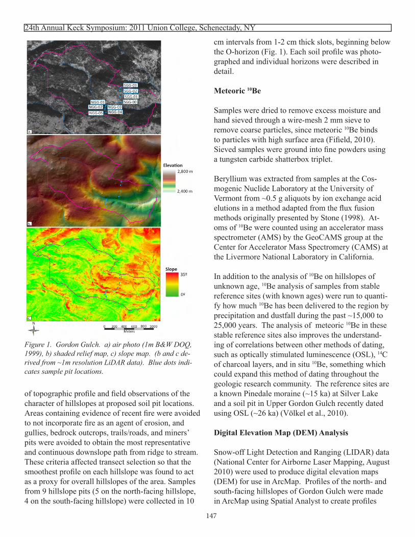
24th Annual Keck Symposium: 2011 Union College, Schenectady, NY
147
cm intervals from 1-2 cm thick slots, beginning below the O-horizon (Fig. 1). Each soil profile was photo-graphed and individual horizons were described in detail.
Meteoric 10Be
Samples were dried to remove excess moisture and hand sieved through a wire-mesh 2 mm sieve to remove coarse particles, since meteoric 10Be binds to particles with high surface area (Fifield, 2010). Sieved samples were ground into fine powders using a tungsten carbide shatterbox triplet.
Beryllium was extracted from samples at the Cos-mogenic Nuclide Laboratory at the University of Vermont from ~0.5 g aliquots by ion exchange acid elutions in a method adapted from the flux fusion methods originally presented by Stone (1998). At-oms of 10Be were counted using an accelerator mass spectrometer (AMS) by the GeoCAMS group at the Center for Accelerator Mass Spectromery (CAMS) at the Livermore National Laboratory in California.
In addition to the analysis of 10Be on hillslopes of unknown age, 10Be analysis of samples from stable reference sites (with known ages) were run to quanti-fy how much 10Be has been delivered to the region by precipitation and dustfall during the past ~15,000 to 25,000 years. The analysis of meteoric 10Be in these stable reference sites also improves the understand-ing of correlations between other methods of dating, such as optically stimulated luminescence (OSL), 14C of charcoal layers, and in situ 10Be, something which could expand this method of dating throughout the geologic research community. The reference sites are a known Pinedale moraine (~15 ka) at Silver Lake and a soil pit in Upper Gordon Gulch recently dated using OSL (~26 ka) (Völkel et al., 2010).
Digital Elevation Map (DEM) Analysis
Snow-off Light Detection and Ranging (LIDAR) data (National Center for Airborne Laser Mapping, August 2010) were used to produce digital elevation maps (DEM) for use in ArcMap. Profiles of the north- and south-facing hillslopes of Gordon Gulch were made in ArcMap using Spatial Analyst to create profiles
of topographic profile and field observations of the character of hillslopes at proposed soil pit locations. Areas containing evidence of recent fire were avoided to not incorporate fire as an agent of erosion, and gullies, bedrock outcrops, trails/roads, and miners’ pits were avoided to obtain the most representative and continuous downslope path from ridge to stream. These criteria affected transect selection so that the smoothest profile on each hillslope was found to act as a proxy for overall hillslopes of the area. Samples from 9 hillslope pits (5 on the north-facing hillslope, 4 on the south-facing hillslope) were collected in 10
Figure 1. Gordon Gulch. a) air photo (1m B&W DOQ, 1999), b) shaded relief map, c) slope map. (b and c de-rived from ~1m resolution LiDAR data). Blue dots indi-cates sample pit locations.

24th Annual Keck Symposium: 2011 Union College, Schenectady, NY
148
(Fig. 2). For each hillslope, the transect with pits was the original profile produced. Transects parallel to these were spaced approximately 120 m apart and extended to the borders of the drainage basin. All transects began in the channel and ended at the ridge and were normal to the channel. Spatial Analyst was also used to produce digital elevation, hillshade, and slope maps using LiDAR data. These two maps and the additional air photo provide three different visual representations of Gordon Gulch drainage basin as a whole (Fig. 2).
RESULTSMap Analysis
The air photo clearly depicts differences in present
vegetation on the north- and south-facing hillslopes of lower Gordon Gulch. Vegetation is less dense on the south-facing hillslope, whereas little except vegeta-tion is visible on the north-facing hillslope. With the addition of a hillshade layer, the DEM de-picts both elevation and topographic features. Bed-rock outcrops are seen extruding 1-10 m above the dominant soil mantled hillslopes. These bedrock out-crops are characterized by shallow slope upslope and close to vertical slope on the downslope sides. The density of bedrock outcrops between the north- and south-facing hillslopes appears similar in upper Gor-don Gulch. However, there is a disparity of bedrock outcrop density between the north- and south-facing hillslopes of lower Gordon Gulch (Trotta, 2010). More bedrock outcrops are present on the south-facing hillslope, and these are larger than those on the north-facing hillslope. The north-facing hillslope is dissected by numerous gullies, whereas few gullies are visible on the south-facing hillslope. The slope map shows that many of the north-facing hillslopes have a parabolic shape in which the highest slopes are in the middle-range of the transect and the lowest slopes at the bottom of the gulch and the drain-age divide. In contrast, the slope is fairly constant on the south-facing hillslope of lower Gordon Gulch, except where the slope increases in the downslope di-rection of bedrock outcrops and as the slope shallows near the ridge of the drainage basin.
Hillslope Profiles
The north-facing hillslope of Gordon Gulch is shorter and shallower (Fig. 2a) than the south-facing hill-slope, which is longer and steeper overall (Fig. 2b). Using data drawn from ArcMap hillslope profiles (Fig. 2) beginning at the first stream encountered and ending at the drainage divide, the average slope of all north-facing hillslopes is 9.6º and of all south-facing hillslopes is 12.2º. Taking the average from the sampled pit transect and the two transects parallel on each side yields slopes of 15.0º on the north-facing hillslope and 19.6º on the south-facing hillslope. The steepest local (and non-bedrock outcrop) slopes are found in the lower half of the north-facing hillslope, as seen in the slope map, but not reflected in profile
Figure 2. Profiles of the north- and south-facing hillslopes of Gordon Gulch extracted from ~1m resolution LiDAR digital elevation model. Profiles are labeled from west to east (downstream) beginning with “A” or “a”. Tran-sects in bold are the focus transects of this study. Open circles indicate locations of pits sampled for meteoric 10Be. Shaded relief map (see Fig 1. for legend) shows approxi-mate location of transects with black lines. Dots indicate sample pit locations. Dashed line indicates approximate boundary between the upper and lower basin.
0
10
20
30
40
50
60
70
80
90
100
110
120
130
140
150
160
170
180
190
800 900 1000100 200 300 400 500 600 700
20
40
60
80
100
120
0
NGG-01NGG-02
NGG-03
NGG-04
NGG-05
0
10
20
30
40
50
60
70
80
90
100
110
120
130
140
150
160
170
180
190
0 100 200 300 400 500 600 700 800 900 1000100 200 300 400 500 600
20
40
60
80
100
120
140
160
180
0
Dis
tanc
e (m
)
Distance (m)
SGG-00
SGG-01
SGG-02
SGG-03
N S
qpr
s
t
o u
v
nk
w j
ihgml
f
e
cd
b
a
VU
W
T
MO N R
PQ S L
K
JI
C
A BHE G
FDM
L
KJID
HE
GF
a. North Facing Hillslope
b. South Facing Hillslope
A BC
DEFG
H IJ
KL M N
O P Q RS T U V
W
a b c de f g
hi j
k
l
mnopq r s t u v w x

24th Annual Keck Symposium: 2011 Union College, Schenectady, NY
149
Pits SGG-01 and SGG-03 appear to be approaching a steady concentration at depth, whereas pits SGG-00 and SGG-02 show no clear indication of approaching a steady concentration.
Silver Lake Moraine
The Silver Lake moraine section shows a bulge pro-file with the highest concentration in the Bw-horizon (Fig. 4a). In the Bw-horizon at 25 cm and 35 cm deep, 10Be concentrations (1.00 x 10⁹ and 9.34 x 10⁸ atoms/g) are greater than twice the next highest con-centration (4.35 x 10⁸ atoms/g) in the Ej-horizon at 15 cm deep (Tab. 1). Concentrations decrease to as low as 2.28 x 10⁷ atoms/g in the Cu-horizon and appear to be approaching a steady concentration.
data due to profile length averages. In lower Gordon Gulch, the north-facing hillslope profiles are charac-terized by a ridge creating a break in slope followed by a second slope ending at the drainage basin bound-ary. The first slope (before the ridge break) is para-bolic in nature. Bedrock outcrops are found almost solely at the top of the profile, but above the break in slope. In contrast, the south-facing hillslope profiles are more linear than parabolic and have a more con-sistent slope from ridge to stream, except where bro-ken by bedrock outcrops. Bedrock outcrops are more abundant on this slope than the north-facing hillslope, and are seen as the many small spikes on the profiles.
Meteoric 10BeLower Gordon Gulch
North-facing hillslope soils have 10Be concentrations of 5-8 x 10⁸ atoms/g in the uppermost samples and decline to < 2 x 10⁸ atoms/g at depths >60 cm (Table 1). Pits NGG-01 and NGG-05 show exponentially declining profiles with some variability and small bulges, corresponding to the highest concentration of 10Be in the B-horizon and the Cox-horizon respec-tively. Pits NGG-02, NGG-03, and NGG-04 show exponentially declining profiles (with some variabil-ity) with peak meteoric 10Be concentrations towards the top of the profiles. The lowest concentration for each pit is at depth, except for NGG-01 in which the lowest concentration is in the Cox2-horizon (Fig. 3a). Pits NGG-01 and NGG-02 decline to a steady con-centration at depth, whereas the other three pits on this hillslope show no clear indication of approaching a steady concentration. South-facing hillslope soils have 10Be concentrations of 2.5-5 x 10⁸ atoms/g near the surface and decline to < 2.7 x 10⁸ atoms/g at depths >32 cm (Table 1). Pits SGG-00 and SGG-02 show approximately linear de-clining profiles. Pit SGG-02 also shows a bulge, cor-responding to the highest concentration of 10Be in the SGG-02 A/Cox1-horizon border. Pit SGG-03 shows an exponentially declining profile with a small bulge, corresponding to the highest concentration of 10Be in the Cox1-horizon. Pit SGG-01 shows no clear declin-ing trend with a bulge corresponding to the highest concentrations of 10Be in the SGG-01A-horizon. The lowest concentration for each pit is at depth (Fig. 3b).
Table 1. 10Be concentration data for samples chosen for this analysis. Preliminary 10Be inventory and soil ages were calculated using equations presented in the text.
Sample 10Be Bulk Density Thickness 10Be inventory Total Pit Inventory Soil Age
(atoms/g) (g/cm^3) (cm) (atoms/cm^2) (atoms/cm^2) (years)
NGG-01-8 8.06E+08 1.2 5 3.69E+09
3.53E+10 32,300
NGG-01-18 8.96E+08 1.4 10 9.77E+09 NGG-01-28 7.54E+08 1.4 25 1.95E+10 NGG-01-58 2.27E+08 1.6 35 2.26E+09 NGG-01-98 2.02E+08 1.6 40 1.06E+09
NGG-01-138 1.47E+08 1.6 45 -2.73E+09 NGG-01-188 2.06E+08 1.6 50 1.50E+10
NGG-02-5 5.73E+08 1.6 10 8.09E+09
2.00E+10 18,300 NGG-02-25 2.74E+08 1.6 25 7.97E+09 NGG-02-55 1.64E+08 1.6 35 4.88E+09 NGG-02-95 1.17E+08 1.6 55 3.41E+09
NGG-02-165 4.07E+07 1.6 70 -4.38E+09
NGG-03-10 5.92E+08 1.5 5 3.42E+09
1.41E+10 12,800 NGG-03-20 3.66E+08 1.5 15 5.23E+09 NGG-03-40 2.61E+08 1.5 20 3.85E+09 NGG-03-60 1.85E+08 1.5 20 1.58E+09
NGG-04-5 5.48E+08 1.4 5 2.87E+09
1.64E+10 15,000 NGG-04-15 4.29E+08 1.4 10 4.10E+09 NGG-04-25 4.50E+08 1.6 10 5.09E+09 NGG-04-35 2.49E+08 1.6 15 2.81E+09 NGG-04-55 1.80E+08 1.6 20 1.53E+09
NGG-05-0 5.56E+08 1.4 5 3.00E+09
2.73E+10 24,900 NGG-05-10 6.62E+08 1.5 10 7.95E+09 NGG-05-20 4.41E+08 1.5 10 4.63E+09 NGG-05-30 5.31E+08 1.6 15 9.57E+09 NGG-05-50 1.98E+08 1.6 20 2.10E+09
SGG-00-0 4.59E+08 1.2 5 1.88E+09
1.53E+10 13,900 SGG-00-10 3.99E+08 1.2 10 3.07E+09 SGG-00-20 3.95E+08 1.6 10 4.21E+09 SGG-00-30 3.12E+08 1.6 15 4.32E+09 SGG-00-50 1.88E+08 1.6 20 1.80E+09
SGG-01-0 2.85E+08 1.2 5 8.82E+08
1.85E+10 16,900 SGG-01-10 3.51E+08 1.2 10 2.52E+09 SGG-01-20 4.28E+08 1.6 15 7.11E+09 SGG-01-40 3.85E+08 1.6 20 8.10E+09 SGG-01-60 1.29E+08 1.6 20 -1.04E+08
SGG-02-2 3.51E+08 1.5 5 1.64E+09
9.42E+09 8,580 SGG-02-12 3.69E+08 1.5 10 3.55E+09 SGG-02-22 2.79E+08 1.5 10 2.20E+09 SGG-02-32 2.67E+08 1.5 10 2.02E+09
SGG-03-0 2.93E+08 1.3 5 1.05E+09
1.19E+10 10,900 SGG-03-10 3.56E+08 1.5 10 3.38E+09 SGG-03-20 2.96E+08 1.5 15 3.72E+09 SGG-03-40 2.08E+08 1.5 25 2.88E+09

24th Annual Keck Symposium: 2011 Union College, Schenectady, NY
150
Upper Gordon Gulch
The soil originally sampled for OSL dating by Jörg Völkel (2010) has a maximum 10Be concen-tration of 1.66 x 10¹⁰ atoms/g near the surface. The concentration decreases to 3.13 x 10⁹ atoms/g at depth (Tab. 1) and creates an exponentially declining profile (Fig. 4b).
Inventory and Soil Age Calculations
Meteoric 10Be inventories IBe (atoms/cm2) were cal-culated using an equation taken from Jungers et al. (2009):
IBe = ∑(CBe-Cinh)ρsh
where CBe is depth-integrated 10Be concentration, Cinh is the inherited component of meteoric 10Be , ρs is depth-integrated soil bulk density, and h is soil thick-ness for each depth subsample.
Inheritance for NGG-01 was assumed as the average concentration of the three deepest samples (1.85 x 10⁸ atoms/g) and for NGG-02 as the average of the two
deepest samples (7.87 x 10⁷ atoms/g). The average of the NGG-01 and NGG-02 inheritance values (1.32 x 10⁸ atoms/g) was used as the value for the remaining NGG pits and the SGG pits. The deepest concentra-tion (9.21 x 10⁷ atoms/g) was used for the OSL-dated pit. Inheritance has not yet been taken into account for the Silver Lake moraine, because it is assumed to be minimal. Bulk soil density was measured in the field for several sample locations and other bulk density values were assumed as standard values for soil and till density. The soil thickness for each depth subsample was calculated by establishing a mid-point between sample locations. The midpoint value was added to bottom samples to account for un-collected soil.
Figure 3. Meteoric 10Be from soils on the north (a.) and south (b.) facing hillslopes of lower Gordon Gulch.
0
20
40
60
80
100
120
140
160
180
200
0 100000000 200000000 300000000 400000000 500000000 600000000 700000000 800000000 900000000 1E+09
SGG-00
SGG-01
SGG-02
SGG-03
0
20
40
60
80
100
120
140
160
180
200
0.00E+00 1.00E+08 2.00E+08 3.00E+08 4.00E+08 5.00E+08 6.00E+08 7.00E+08 8.00E+08 9.00E+08 1.00E+09
NGG-01
NGG-02
NGG-03
NGG-04
NGG-05
!"
#!"
$!"
%!"
&!"
'!!"
'#!"
'$!"
'%!"
'&!"
#!!"
!(!!)*!!" '(!!)*!&" #(!!)*!&" +(!!)*!&" $(!!)*!&" ,(!!)*!&" %(!!)*!&" -(!!)*!&" &(!!)*!&" .(!!)*!&" '(!!)*!."
/001!'"
/001!#"
/001!+"
/001!$"
/001!,"
NGG-01
NGG-02
NGG-03
NGG-04
NGG-05
SGG-00
SGG-01
SGG-02
SGG-03
2.00 × 10⁸ 4.00 × 10⁸ 6.00 × 10⁸ 8.00 × 10⁸
2.00 × 10⁸ 4.00 × 10⁸
20
60
100
140
0
20
180
60
0
Dep
th (c
m)
Meteoric ¹⁰Be Concentration(atoms/g)
a. North Facing Hillslope
b. South Facing Hillslope
0
50
100
150
200
250
300
350
0 200000000 400000000 600000000 800000000 1E+09 1.2E+09
0
20
40
60
80
100
120
0 100000000 200000000 300000000 400000000 500000000 600000000
2.00 × 10⁸ 4.00 × 10⁸ 6.00 × 10⁸ 8.00 × 10⁸ 1.00 × 10⁹
1.00 × 10⁸ 2.00 × 10⁸ 3.00 × 10⁸ 4.00 × 10⁸ 5.00 × 10⁸
50
100
150
200
250
300
20
40
60
80
100
Dep
th (c
m)
0
0
Meteoric ¹⁰Be Concentration(atoms/g)
Meteoric ¹⁰Be Concentration(atoms/g)
Dep
th (c
m)
a. Silver Lake Moraine
b. Upper Gordon Gulch OSL Dated Pit
Figure 4. Meteoric 10Be concentration plots for the Silver Lake moraine (a.) and upper Gordon Gulch pit dated with OSL (b.).

24th Annual Keck Symposium: 2011 Union College, Schenectady, NY
151
Soil ages (t, in years) were calculated for each pit us-ing an equation adapted from Graly et al. (2010):
t = (-1/λ)ln(1-λIBe/q)
where λ is the 10Be disintegration constant (5.1 x 10⁻⁷), IBe is the total inventory of 10Be (atoms/cm2), and q is the local annual meteoric 10Be flux (atoms/cm2). The value of q was estimated from Figure 4 of Graly et al. and according to an annual precipitation rate of ~45 cm in Gordon Gulch (1.1 x 10⁶ atoms/cm2) and ~90 cm at Silver Lake (1.8 x 10⁶ atoms/cm2), both at ~40º latitude, (Graly et al., 2010).
DISCUSSION
Meteoric 10BeLower Gordon Gulch
Meteoric 10Be data suggest that the two opposite fac-ing hillslopes of lower Gordon Gulch are evolving differently (Fig. 3). The three soil pits in the middle of the transect on the north-facing hillslope all show declining profiles of meteoric 10Be concentration, sug-gesting an eroding slope because upper soil has been stripped from the column and 10Be has not had the time to concentrate in a certain layer. Potential expla-nations for small bulges in the lowest (NGG-01) and highest (NGG-05) profiles include their locations and horizon profiles. Pit NGG-05 is located above the major break in slope on the hillslope, and therefore represents a different environment than the four lower pits. The highest concentrations of meteoric 10Be in pits NGG-01 and NGG-03 are in the B-horizons. Meteoric 10Be concentration data obtained from the south-facing slope differs from the concentrations from the north-facing slope. The only declining pro-file of the four sampled pits is the lowest (SGG-00), whereas the other profiles all contain a small bulge. Preliminary analysis suggests that perhaps the upper portion of the soil column on the south-facing hill-slope has been stripped and evacuated. Had this not occurred, the profile shape on the south-facing hill-slope may have resembled those on the north-facing hillslope with small bulges but overall decline profiles
and greater inventories. Therefore consistent mete-oric 10Be concentration profile shapes across the two opposite facing hillslopes of Gordon Gulch would have been seen. Preliminary 10Be inventory calculations show dif-ferences between the two hillslopes (Table 1). The north-facing hillslope has a greater inventory than the south-facing hillslope, particularly in the upper ~30 cm of the profiles. Preliminary soil age calculations (Table 1) correlate to inventory differences and sug-gest that the south-facing hillslope of lower Gordon Gulch is eroding faster than the north-facing hillslope.
Upper Gordon Gulch
The 10Be profile shows a declining profile (Fig. 4b), suggesting a young, eroding landscape. The prelimi-nary soil age calculation drawn from an inventory of 2.43 x 10¹⁰ atoms/cm2 suggests an age of ~22,200 years (Table 1), matching the age obtained from OSL dating of the same soil profile (~26,500 years) (Völkel et al., 2010).
Silver Lake
The 10Be profile shows a bulge profile (Fig. 4a) with the highest 10Be concentration in the Bw-horizon, fur-ther emphasizing a correlation between 10Be and Fe-rich B-horizons from previous studies. Preliminary soil age calculations suggest an age of ~54 ka (Table 1), older than the known age of this moraine at ~15ka.
Sources of Error
Potential sources of error in all inventory and soil age calculations include lack of soil bulk density measure-ments, estimated annual 10Be flux rates, and estimated 10Be inheritance. Inheritance also comes into question when contemplating what this may mean for hillslope evolution. Additionally, some pits may not have been dug deep enough to sample the entire meteoric 10Be inventory, due to regolith and potential bedrock com-position.

CONCLUSION
More detailed analysis of processes, soil ages, mete-oric 10Be flux, and 10Be inventories will lead to further analysis and discussion of the differences between the north-and south-facing hillslopes of Gordon Gulch and more precise dating of Gordon Gulch hillslopes and the Silver Lake moraine. Preliminary age cal-culations show that Gordon Gulch regolith is latest Pleistocene or Holocene in age or younger, not evolv-ing throughout the Cenozoic, and that the soil flux here is rapid.
ACKNOWLEDGEMENTS
Many thanks to the KECK consortium and Amherst College for funding and support. Thank you Will Ouimet and David Dethier for continuing excitement and advice. Thank you to Peter Crowley for learning a completely new subset of geology to become an effective replacement advisor. Thank you to all my fellow CO-KECK students, particularly the awesome soils group. Lastly, thank you to the many people from CU-Boulder, UMass, UVM, and the GeoCAMS group at the Livermore National Laboratory who helped in many different steps of field and laboratory work.
REFERENCES
Anderson, R. S., Riihimaki, C. A., Safran, E. B., MacGregor, K. R., 2006, Facing reality: Late Cenozoic evolution of smooth peaks, glacially ornamented valleys and deep river gorges of Colorado’s Front Range: in Willett, S.D., Hov-ius, N., Brandon, M.T., and Fisher, D.M., eds., Tectonics, climate and landscape evolution: Geo-logical Society of America Special Paper 398, p. 397-418.
Fifield L. K., Wasson R. J., Pillans B., Stone J. O. H., 2010, The longevity of hillslope soil in SE and NW Australia, CATENA, Volume 81, Issue 1, p. 32-42.
Graly, J. A., Bierman P. R., Reusser, L. J., Pavich, M. J., 2010, Meteoric 10Be in soil profiles - A
152
24th Annual Keck Symposium: 2011 Union College, Schenectady, NY
global meta-analysis, Geochimica et Cosmochi-mica Acta, v. 74, Issue 23, p. 6814-6829.
Jungers, M. C., Bierman, P. R., Matmon, A., Nich-ols, K., Larsen, J., and Finkel, R., 2009, Tracing hillslope sediment production and transport with in situ and meteoric 10Be, J. Geophys. Res., v. 114.
Stone, J., 1998, A rapid fusion method for separation of beryllium-10 from soils and silicates: Geochi-mica et Cosmochimica Acta, v. 62, p. 555–561.
Trotta, J. R., 2010, The Distribution of Tors in Gordon Gulch, Front Range, Colorado. Thesis submit-ted in partial fulfillment of the requirements for the Degree of Bachelor of Arts with Honors in Geosciences, Williams College.
Völkel, J., Huber, J., Leopold, M. and Dethier, D., 2010, Young Quaternary slope sediments and paleosoils in the Colorado Front Range – process and age, Geological Society of America Ab-stracts with Programs, 42, no. 5, p. 469.
Willenbring, J. K. and von Blanckenburg, F., 2010, Meteoric cosmogenic Beryllium-10 adsorbed to river sediment and soil: Applications for Earth-surface dynamics, Earth Science Reviews v. 98, p. 105-122.