Inventory changes and future returns - Faculty...

Inventory changes and future returns

December, 2001 (First version: March 1999)

by

Jacob K. Thomas†

and

Huai Zhang§

† Corresponding author: 620 Uris Hall, Columbia Business School, New York, NY. 10027. Tel: (212) 854-3492, e-mail: [email protected]. § University of Illinois at Chicago, Chicago, IL 60607 We received helpful comments from anonymous referees, Mary Barth, Sudipta Basu, Mary Ellen Carter, John Elliott, Paul Hribar, Mike Kirschenheiter, Andy Leone, Jing Liu, David Mest, Mark Nelson, Doron Nissim, Zoe-Vonna Palmrose, Steve Penman, Scott Richardson, Steve Ryan, Richard Sloan, Sarah Tasker, Ross Watts, Ira Weiss and workshop participants at the 2001 RAST conference (at Cornell University), 12th Annual Conference on Financial Economics and Accounting (at Rutgers University), University of California-Berkeley, Columbia University, London Business School, University of Maryland, University of Missouri-Columbia, University of Nebraska, and University of Southern California.


ABSTRACT

We find that the negative relation between accruals and future abnormal returns documented by

Sloan (1996) is due mainly to inventory changes. We propose three explanations for this result,

derived from the prior literature, but find evidence inconsistent with all three explanations. To

assist future investigations in formulating additional explanations, we document several

empirical regularities for extreme inventory change deciles. We speculate that demand shifts

explain our results, and examine the feasibility of alternative reasons for the stock market’s

apparent inability to recognize the impending profitability reversals. Our evidence is consistent

with earnings management masking the implications of demand shifts.


Sloan (1996) documents a startling finding: investing long/short in firms in the

bottom/top decile of accruals (scaled by average beginning and ending total assets) generates a

hedge portfolio return of about 10 percent in the following year, and about 5 percent and 3

percent in the two years after that. He concludes that the stock market fails to recognize that

accruals and cash flows, the two components of reported earnings, have different persistence. As

a result, firms with high (low) accruals, or low (high) cash flows, report earnings in the following

year that are predictably lower (higher) than market expectations, and stock prices move

accordingly. This result has been investigated extensively in the recent literature, and the

collective evidence suggests that while managers recognize the implications of accruals (e.g.,

Beneish and Vargus 2001), stock prices and relatively sophisticated stock market participants do

not (e.g., Bradshaw, Richardson, and Sloan 2001).

Our first objective is to identify the components of Sloan’s accrual measure that are

primarily responsible for this apparent market inefficiency. We find that inventory changes

represent the one component that exhibits a consistent and substantial relation with future

returns. Our second objective is to understand how inventory changes, a seemingly innocuous

item (since inventory acquisitions represent accruals that affect operating cash flows but not

earnings), are linked to subsequent abnormal returns. We first propose three explanations with

testable predictions, which are derived from results documented in the prior literature, but find

evidence inconsistent with all three explanations. We then switch to documenting empirical

regularities and fashioning an explanation that is potentially consistent with our evidence. Since

limitations of available data hamper our efforts to directly test this conjecture, our contribution

lies in laying the groundwork for subsequent investigations.

2

The following are some key empirical regularities we document for extreme inventory

change firms. First, firms with inventory increases (decreases) experience higher (lower)

profitability, growth, and stock returns over the prior five years, but those trends reverse after the

extreme inventory change. Second, firms with inventory increases (decreases) experience

inventory decreases (increases) in the prior year, even though profitability increases (decreases)

in both years. Third, the abnormal returns observed after the inventory changes are concentrated

at subsequent quarterly earnings announcements and are related to predictable earnings

“surprises” reported at those announcements. Fourth, quarterly COGS/Sales and SG&A/Sales

exhibit similar patterns, including unusual fourth quarter changes.1 Fifth, LIFO firms with

inventory increases represent one subgroup of extreme inventory change firms that exhibits

abnormal return and profitability patterns unlike those observed for other firms. Finally,

abnormal returns are observed for extreme deciles of changes in all three inventory

components—raw material (RM), finished goods (FG) and work-in process (WIP)—with the

highest abnormal returns observed for changes in RM inventory.

We conjecture that demand shifts cause both the inventory changes and related

profitability reversals we observe. Firms with prior increases (decreases) in profitability and

demand are projected to continue that trend, but for some of these firms actual demand may fall

short of (exceed) projected demand, and this imbalance between sales and production/purchases

results in inventory increases (decreases). Demand shifts for these firms presage a reversal in

profitability trends, but the stock market does not fully recognize this reversal until the following

year because the implications of the demand shift are not revealed in contemporaneous reported

profitability. We consider earnings management and the impact of varying production levels on

1 COGS, represents Cost of Goods Sold (or manufacturing costs, incurred in-house and/or paid to suppliers), and

SG&A, represents Selling, General, and Administrative (or non-manufacturing) expenses.

3

fixed manufacturing overhead absorbed in COGS (e.g., Jiambalvo, Noreen, and Shevlin 1995) as

potential reasons why the impending reversals are masked in reported profitability.

This paper is related to the extensive recent literature that has probed various aspects of

the Sloan (1996) result and generally confirmed its robustness (e.g., Ahmed, Nainar, and Zhou

2001, Ali, Hwang, and Twombley 2000, Barth and Hutton 2001, Bradshaw, Richardson, and

Sloan 2001, Collins and Hribar 2001 and 2002, Fairfield, Whisenant and Yohn 2001, Richardson

and Tuna 2001, Richardson et al. 2001, Tarpley 2000, and Xie 2001). Three studies, Hribar

(2000), Chan et al. (2001) and Zach (2001), also consider the impact of inventory changes.2

We describe our samples and variables in section 1 and document support in section 2 for

our claim that Sloan’s result is due primarily to inventory changes. In section 3, we examine the

three explanations that are derived from results in prior studies. Section 4 contains the empirical

regularities we uncover for extreme inventory change firms, and section 5 discusses our demand

explanation. Section 6 concludes.

1. Samples and variables

Our sample extends from 1970 to 1997 (years as defined by Compustat) and consists of

39,315 observations. Financial statement (stock return) data are obtained from the 1998 (1999)

edition of Compustat (CRSP). To maintain consistency with Sloan (1996), we include only

NYSE and AMEX firms, and use the same variable definitions (details of all variables used in

this study are provided in the Appendix).3 We require that the following data items be non-

missing for a firm-year to be included in our sample: accruals as defined in Sloan (1996), change

in accounts payable, change in accounts receivable, depreciation expense, change in inventory,

2 Despite differences across studies in the samples studied and methodologies employed, the robustness of our

primary finding regarding the importance of inventory changes is confirmed in all studies. 3 Exchange membership provided in Compustat relates only to the status as of 1998, whereas the CRSP event file

provides the history of exchange membership. We use CRSP membership data when building our sample.

4

next year’s earnings and 12-month size-adjusted returns (described below). For many of our

tests, we use decile ranks for the different independent variables, to reduce the impact of outliers

and to maintain consistency with the prior literature examining accrual anomalies. These decile

ranks are constructed based on each year’s distribution.4

Size-adjusted return (SAR) represents the difference between the firm’s buy-and-hold

return and the buy-and-hold return on a value-weighted portfolio of firms in the same CRSP size

decile. Size deciles are determined by the distribution of market values of all NYSE/AMEX

firms at the beginning of the calendar year. SARs are computed over two holding periods: a) 12-

month holding periods, beginning four months after the fiscal year end, and b) 3-day windows

around quarterly earnings announcements including the day before, the day after, and the day of

the earnings announcement (as reported in Compustat).

Given the volume of results generated, we only report details of the most important

results. Other results are summarized where relevant and details of those results are available

upon request. Also, given the descriptive nature of the empirical regularities in section 4, we

eschew tests of statistical significance for that evidence and find it convenient to present some of

it as plots, rather than in tabular form.

2. Importance of inventory changes

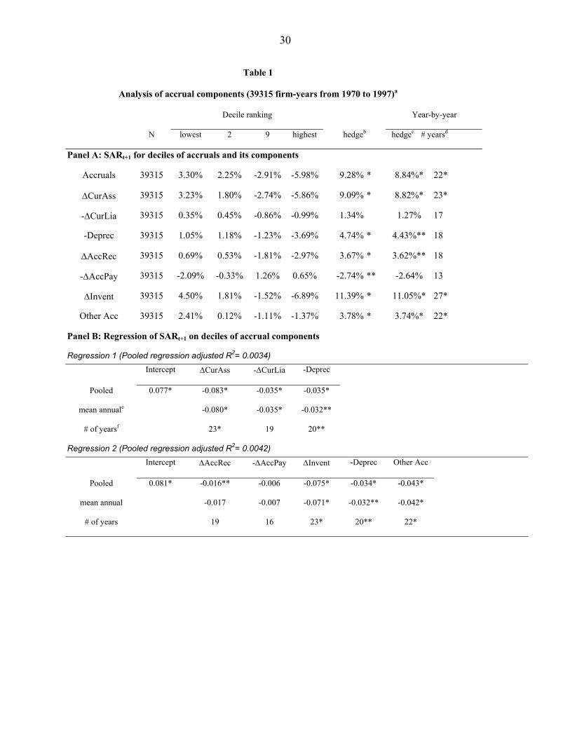
The first row in Table 1, Panel A, provides the mean size-adjusted abnormal returns

(SARt+1) earned by different accrual deciles over the 12 month period beginning 4 months after

year 0. The 4 columns labeled “lowest” to “highest” provide the mean SARt+1 earned over the

pooled sample for the two bottom and two top deciles. (The six intermediate deciles exhibit

4 These distributions, which combine firms from the same year as defined by Compustat (fiscal years ending

between June of this year and May of the following year), are not available to form portfolios until all firms have reported their annual results. While this is a potential source of bias, extensive sensitivity analysis we conducted suggests that in fact there is little bias created. See also Tarpley (2000).

5

abnormal returns that vary monotonically between the two extremes, and are not reported here

for brevity.) These SARt+1 range from a mean of 3.3 percent for the most negative accruals to a

mean of –5.98 percent for the most positive accruals. The mean SARt+1 for the lowest decile

minus the mean SARt+1 for the highest decile, which is 9.28 percent, is reported under the

“hedge” column. The value of 8.84 percent reported under the “year-by-year hedge” column

provides the mean of the 28 annual hedge returns earned in each sample year, and the value of 22

under the “# years” column indicates that the hedge returns are positive in 22 out of 28 years.

The indicated statistical significance of the mean annual hedge return (# of years), which is

determined by a t-test (sign test) based on the magnitude (sign) of the 28 annual hedge returns,

confirm that the returns are significant at the 1 percent level. These results are consistent with

those reported in Sloan (1996).

To identify the components of Sloan’s accrual measure that are relatively more important

for his result, we report SARt+1 for deciles of different accrual components. Items that appear

with a negative sign in the accrual measure (e.g. depreciation) are multiplied by –1 to align the

sign of hedge returns across components. Given potential correlation among the different

accruals components, these univariate results are for illustrative purposes and help to identify the

component that provides the largest and most consistent abnormal returns; the partial effect of

each component is better described by the regression results discussed later.5

The next three rows in Panel A consider an initial partition of Sloan’s accrual measure:

changes in non-cash current assets (∆CurAss), minus changes in current liabilities other than

taxes payable and the current portion of long-term debt (-∆CurLia), and minus depreciation and

5 Examination of pairwise correlations among accruals and the different accrual components considered suggest

that accruals are most closely related to changes in accounts receivable and inventories, and depreciation. While most pairwise correlations between accrual components are significant, the strongest correlations observed are between changes in accounts receivable and inventories.

6

amortization (-Deprec), all scaled by average total assets. Changes in current assets generate the

highest hedge returns in year +1, and appear to be the component that is the primary source of

abnormal returns for Sloan’s accrual measure. The hedge returns and year-by-year results are

similar to those reported for accruals. While the sign of the hedge returns for changes in current

liability are consistent with those observed for accruals, the smaller magnitudes reported (hedge

return of 1.34 percent), the fewer # of years (17 out of 28 years) with positive hedge returns, and

the lack of statistical significance suggest this component is relatively unimportant for Sloan’s

result. Finally, while the depreciation deciles exhibit statistically significant returns consistent

with the accrual strategy, the magnitude of the hedge portfolio returns and the # of years with

consistent hedge returns are less convincing than those for current asset changes.

To further probe the source of abnormal returns earned by accrual portfolios, we examine

portfolios based on deciles of the following individual current asset and current liability

accounts: changes in accounts receivable (∆AccRec), inventory (∆Invent), and all other items of

current accruals ( Other Acc), and minus changes in accounts payable (-∆AccPay). The results

reported in the next four rows of Table 1, Panel A, suggest that inventory changes represent the

component of accruals that provides the largest hedge returns. Not only are these hedge returns

larger than those for accruals (11.39 percent versus 9.28 percent), the hedge return is positive in

27 of the 28 years examined.6 While the negative hedge returns earned by the accounts payable

deciles appear inconsistent with the Sloan hypothesis, the regression results reported next

indicate that this is due to omitted correlated accrual components.

6 The lone year with negative hedge returns (of –4 percent) is 1983. We were unable to discern a relation between

the magnitude of hedge returns in each year and various potentially relevant factors, such as economic conditions and the cutoff values used to form extreme inventory change deciles.

7

The results of estimating regressions of SARt+1 on different accrual components are

reported in Panel B, of Table 1.o allow comparisons with the hedge portfolio results in Panel A,

the deciles of the different regressors are transformed to range between 0 (lowest) and 1

(highest). Ignoring correlations among regressors, this regression analysis is equivalent to

examining hedge returns (with the signs reversed, since hedge returns are based on SARt+1 for

the lowest minus SARt+1 for the highest decile), provided abnormal returns are related linearly to

the different decile ranks. Since the abnormal returns/decile rank relations are in fact non-linear,

the hedge portfolio returns deviate from the regression coefficients. For example, estimating a

bivariate regression of abnormal returns on the inventory change deciles results in a lower slope

(7.26 percent) than the hedge return reported in Table 1 (11.39 percent). In Panel B, we report

the coefficients from pooled regressions, the mean of the coefficients from annual regressions,

and the # of years that the coefficient in the annual regressions has a negative sign.

The results of regression 1 confirm the importance of changes in current assets, relative

to changes in current liabilities and depreciation, when explaining variation in SARt+1. The

pooled coefficients are consistent with the year-by-year results (mean annual coefficients and #

of years with negative sign) and these results are generally comparable to the corresponding

hedge results reported in Panel A. Moving to the accrual components considered in regression 2,

again the overall tenor of the results reported in Panel A is maintained. While the coefficient of

7.5 percent on change in inventory is considerably lower than the 11.39 percent hedge return in

Panel A, that difference is due entirely to the above-mentioned nonlinear relation between

abnormal returns and inventory deciles, not due to the presence of other accrual components in

the multiple regression. Note that the coefficient on changes in accounts payable is now negative

8

(though insignificant) indicating that the negative hedge returns obtained in Panel A for this

component are due to correlation with other accrual components.

We repeat the regression analyses reported in regression 2 using the Mishkin (1983) test

framework. Sloan (1996) and Hribar (2000) both use this framework to a) determine the

implications of accruals and its components in year 0 for earnings in year +1, and b) check if

market prices reflect correctly those implications. Those papers provide additional details of the

test and the inferences that can be drawn. Our results confirm our conclusion that the market

misinterprets the implications of inventory changes, and abnormal returns are best explained by

this accrual component. Specifically, the permanence of inventory changes, measured by the

coefficient in the earnings regression (=0.0236), is much smaller than the market’s assessment of

that permanence, measured by the coefficient in the returns regression (=0.183). In effect the

market assumes that the earnings impact of inventory changes is substantially more permanent

than it actually is. While some of the comparisons for other accrual components are also

statistically significant, the inventory change component is clearly the most significant (largest

test statistic) and appears to be the most important driver of the mispricing documented by Sloan.

3. Testing explanations for inventory results derived from prior research

We consider three potential explanations for our inventory result, each of which is based

on results of prior research that identify a less visible factor which is associated with profitability

reversals and future abnormal returns. We consider the possibility that the observed relation

between inventory changes and subsequent abnormal returns is because inventory changes are

correlated with these factors. While the first explanation is derived from research unrelated to the

mispricing of accruals, the remaining two explanations are derived from research that proposes

alternative explanations for Sloan’s finding regarding accruals predicting abnormal returns.

9

The first explanation is based on Titman, Wei, and Xie (2001), which documents a

negative relation between capital expenditures and subsequent abnormal returns. They conclude

that firms with high (low) profitability in prior periods generate more (less) free cash flows,

which results in reduced (increased) future profitability and negative (positive) abnormal returns

because of increased (reduced) investments in negative net present value capital expenditures.

Second, the results reported in Fairfield, Whisenant, and Yohn (2001) suggest that accruals

(primarily working capital accruals) are related positively to changes in net operating assets,

which are in turn negatively related to future profitability. Finally, Tarpley (2000) investigates

the possibility that positive (negative) accruals follow periods of high (low) growth, that the

stock market erroneously extrapolates those growth rates into the future, and stock returns

decline (increase) predictably when growth rates mean revert.

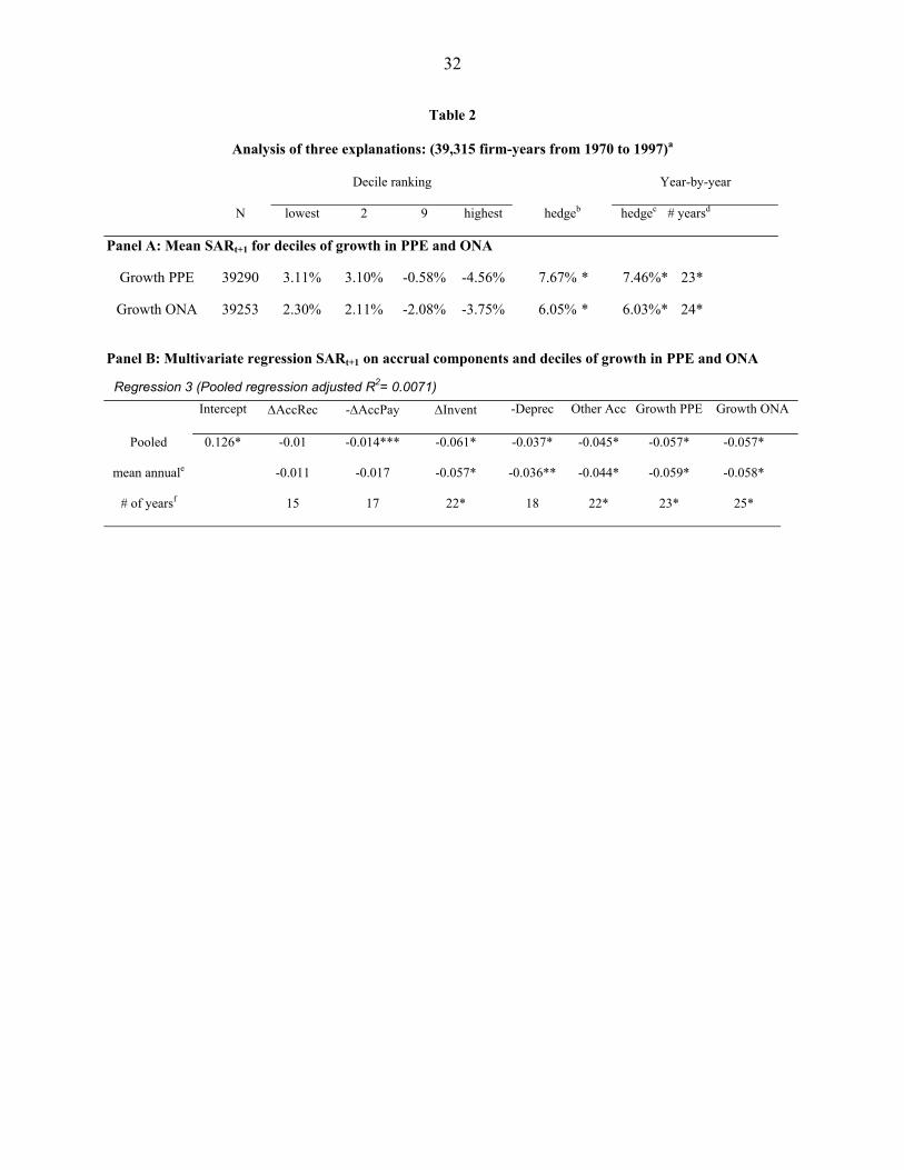
To investigate the first two explanations, we report in Panel A of Table 2 the abnormal

returns earned by decile portfolios formed using growth in net plant, property and equipment

(PPE) and growth in net assets other than PPE and working capital (ONA). We observe fairly

large hedge portfolio returns (7.67 percent and 6.05 percent for PPE and ONA, respectively) and

remarkably consistent year-by-year performance (23 and 24 years out of 28). We confirm that

these two measures of noncurrent accruals are in fact positively correlated with inventory

changes. To test the separate ability of inventory changes to predict future abnormal returns, after

controlling for these two non-operating accruals, we estimate regression 3, reported in Panel B of

Table 2, which includes deciles of these two noncurrent accrual measures to the components of

accruals considered in regression 2 (reported in Table 1, Panel B). While the pooled coefficient,

mean of annual coefficients, and the number of years with significant mean coefficients for the

inventory change variable decline slightly from the levels reported in regression 2, they remain

10

large and significant. Interestingly, growth in PPE and growth in other net assets are also equally

important. These results suggest that although growth in both PPE and other net assets predict

future abnormal returns, those relations are separate from the relation between inventory changes

and abnormal returns we claim drives the Sloan result.

Consistent with the second explanation that relies on a negative relation between changes

in entity size and profitability shifts, Zach (2001) argues that a portion of the Sloan result is due

to increases (decreases) in working capital accruals derived from balance sheet numbers

reflecting mergers/acquisitions (divestitures), which in turn appear to be related to subsequent

increases (decreases) in profitability.7 To investigate the possibility that our inventory change

results are due to acquisitions and divestitures, we examine abnormal returns for inventory

deciles for three subgroups (based on Compustat footnote AFTNT 1): those with

mergers/acquisitions, those with divestitures, and those with neither. Consistent with the more

extensive analysis of this potential methodological bias carried out by Zach (2001) for accrual

deciles, we find very similar negative inventory change/abnormal return relations across all three

subgroups. We also formed deciles based on changes in the ratio of inventory to total assets, to

eliminate the correlation between our inventory change measure and entity changes. Despite the

dampening effect caused by changes in noncurrent assets being negatively related to future

abnormal returns (since noncurrent assets are reflected in total assets, the scaling variable), we

find significant abnormal returns that are about half the returns for ∆Invent in Table 1, Panel A.

To investigate the third explanation, relating to the stock market overestimating

(underestimating) future growth for high (low) growth firms, we considered the both historic and

forecasted growth rates but could only discern a weak ability to predict future returns: the hedge 7 We confirm the results of prior research (e.g. Hribar 2000) that similar abnormal returns are observed when

portfolios are formed based on inventory changes from the cash flow statement (available only for years after 1987), which are less likely to be biased by entity changes than the balance sheet changes we consider.

11

returns for extreme growth deciles were uniformly low, and in regression analyses, we observed

insignificant coefficients on growth. More important, there is little impact on the regression

coefficient on inventory changes. As an aside, we find that the relation between inventory

changes and abnormal returns is a function of forecast growth. Specifically, hedge returns for

extreme inventory deciles are smaller for firms with low forecasted growth in earnings per share.

Tarpley (2000) reports a similar finding regarding the interaction between growth and the

accruals/abnormal return relation.

4 Empirical regularities associated with extreme inventory change deciles

In the absence of promising explanations for the relation we document between inventory

changes and abnormal returns, we focus on extreme inventory change deciles and seek to

establish some descriptive features of those firms. These regularities should assist future research

in formulating additional explanations. We provide evidence on the annual (between years –5

and +2) and quarterly (between years –1 and +2) time-series of profitability, growth, and

abnormal returns for these two groups in sections 4.1 and 4.2, respectively. Some other

regularities are reported in Section 4.3.

4.1 Annual time-series

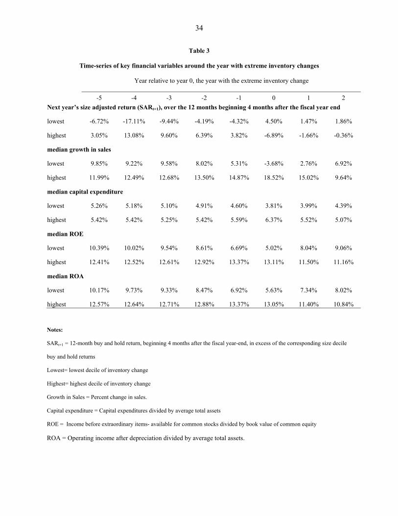
The abnormal returns reported in the first two rows of Table 3 indicate a reversal around

year 0 in the abnormal returns of firms with extreme inventory changes. Note that the abnormal

returns refer to the 12-month period that begins 4 months after the end of that year. For example,

the abnormal returns under year 0 correspond approximately to the period referred to as year +1.

The extreme inventory increase (decrease) group exhibits large positive (negative) abnormal

returns in the 12-month period after years –4 and –3, which then decline for the 12-month period

after years –2 and –1. A sharp reversal is clearly evident in the 12-month period after year 0.

While the magnitudes of these abnormal returns for the lowest decile are similar to those

12

reported for the period following years –2 and -1, the magnitudes for the highest decile are

slightly higher than (similar to) those following year -2 (year –1). The magnitudes of abnormal

returns then decline over the 12-month period following years +1 and +2.

To understand the determinants of this sharp reversal in stock returns, we provide in

Table 3 the median values for two growth measures, for sales and capital expenditures, and two

profitability measures, return on equity (ROE) and return on assets (ROA), for the two extreme

inventory deciles.8 Note that the year 0 numbers, especially for sales growth and capital

expenditures, are unreliable because the selection of extreme inventory change groups tends to

include a disproportionate number of firms making acquisitions (divestitures) in the inventory

increase (decrease) group. The two profitability measures exhibit trends similar to those reported

for the abnormal returns, especially the reversal around year 0. (Recall that the abnormal returns

refer to the 12-month period following that year and should be aligned with the growth and

profitability measures for the next year.) The two growth measures also exhibit similar trends

prior to year 0, but the growth trends seem to extend for one more year, before reversing.

4.2 Quarterly time-series

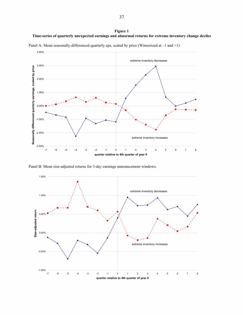
To obtain a better understanding of the stock price movements around year 0, we plot in

Figure 1, Panel A, seasonally differenced quarterly earnings, scaled by end of quarter stock price,

for the quarters around year 0. This measure serves as a simple proxy for the unexpected

component of earnings reported in those quarters. To smooth the effect of outliers, we Winsorize

values above +1 (below –1) to +1 (-1). The inventory increase group exhibits values slightly

above zero indicating small but sustained increases in quarterly earnings during years –1 and 0.

The inventory decrease group exhibits values considerably below 0, indicating sustained declines

8 The mean results are fairly similar and not reported here. Also, we examined a variety of other financial ratios

and obtained results similar to the representative measures reported here.

13

of considerable magnitude over those two years. The two patterns reverse after year 0, with the

inventory increase (decrease) firms showing profitability declines (sharp increases) over year +1,

culminating in the largest changes in the fourth quarter of year +1. The trend continues over year

+2, but the magnitudes are considerably lower than those in year +1.

Examination of the size-adjusted returns around 3-day quarterly earnings announcement

windows, plotted in Panel B of Figure 1, provides the following results. When calibrating the 3-

day announcement window returns, note that announcement window returns are positive on

average (e.g., Ball and Kothari 1991); i.e. the appropriate benchmark to determine positive and

negative news is the unconditional mean of about 0.33 percent, not zero. First, the patterns

observed for these 3-day returns resemble approximately the patterns in Panel A, indicating that

seasonally-differenced quarterly earnings correspond roughly to the stock market’s perceived

earnings surprises. Second, even though the abnormal returns during year 0 continue their

historic trend, stock prices for inventory decreases begin to anticipate the upcoming reversal by

the fourth quarter of year 0. Finally, the stock price reversal observed during years +1 and +2

appears to be related to disclosures made during the corresponding quarterly earnings

announcement window, because a disproportionately high fraction (over 30 percent) of the

annual abnormal returns (reported as SARt+1 under years 0 and +1 in Table 3) is concentrated in

the corresponding four quarterly windows.

We turn next to the quarterly time-series of unexpected changes in COGS and SG&A,

scaled by Sales. In addition to describing quarterly trends in profit margins around year 0, where

margins represent one component of the earnings surprises reported in Figure 1, Panel A, these

14

two measures offer evidence of potential earnings management.9 Specifically, earnings

management is supported by unusual patterns consistent with hypothesized incentives, especially

if they occur around fourth quarters and if similar patterns are observed for both COGS and

SG&A. Based on our finding that a seasonal random walk model (without drift) consistently

describes both ratios better than other time-series models we considered, we use seasonal

differences to measure unexpected variation in quarterly levels of both ratios.10

Seasonally differenced quarterly COGS/Sales and SG&A/Sales could deviate from zero

because of factors other than earnings management. First, both ratios are affected by variation in

selling prices, which could reflect exogenous demand shifts or endogenous pricing decisions

designed to influence demand. Second, to the extent that COGS and SG&A contain fixed

elements that do not vary much from year to year with variation in units produced and sold,

respectively, changes in units produced and units sold affect seasonal differences in both ratios.

Third, to the extent that some items of COGS and SG&A for interim quarters reflect estimates,

variation in interim quarters should be less than that in the fourth quarter, when adjustments are

made for deviations between estimates and actual amounts for such items. Note that while these

factors might often cause random variation in seasonal differences for both ratios, in certain

cases these factors could cause patterns similar to those expected for earnings management:

unusual fourth quarter variation and similar patterns for COGS and SG&A.

9 Traditional measures of earnings management that are based on estimated discretionary accrual measures are

unlikely to be useful in this case because of the high correlation between our inventory change measure and those measures of discretionary accruals.

10 We examined plots of both ratios for different subsamples and determined a distinct seasonal pattern with the ratios being relatively similar across the interim quarters for each firm, but substantially lower in the fourth quarter. We estimated a variety of seasonal quarterly time-series models, and examined the distribution of forecast errors for bias and precision.

15

Figure 2, Panels A and B provide the median ratio of seasonal differences at the quarterly

level for COGS/Sales and SG&A/Sales for the two extreme inventory deciles.11 The results in

Panel A suggest an increase (decrease) in COGS/Sales for the inventory decrease (increase)

group that extends to the fourth quarter of year 0, and a reversal after that.12. Consistent with the

abnormal return patterns noted in Panel B of Figure 1, the profit reversal for inventory decreases

is evident slightly earlier: it occurs in the fourth quarter of year 0, rather than in the first quarter

of year +1.The most striking aspect of these plots is the accentuated patterns observed at the

fourth fiscal quarters, especially in years –1 and +1.

To understand better the interpretation of these plots, consider the COGS/Sales plot for

inventory increases. The ratio declined in each quarter of year –1, relative to the same fiscal

quarter in year –2, with the largest decline (of approximately 0.5 percent of sales) occurring in

the fourth quarter of year –1 (labeled quarter –4). The ratio continued to decline in all four

quarters of year 0. While the magnitudes of declines are smaller than those in year –1, this plot

indicates that profit margins continued to increase in year 0 from their elevated levels in year –1,

which in turn were higher than those in year -2. In particular, even though the changes observed

during the fourth quarter of year 0 are small, about –0.2 percent of sales, this implies that the

unusually low COGS/Sales ratio achieved in the fourth quarter of year –1 is again achieved, and

even lowered further slightly. The profit margin gains earned during years –1 and 0 are for the

most part surrendered in the four quarters of year +1, indicated by the large increases in

COGS/Sales in quarters +1 to +4.

11 To determine the statistical significance of these unexpected changes in the ratios, we computed the p-values

associated with the sign-rank test for each point in Figure 2. Most of the points are associated with very significant p-values. Similar results are observed when examining mean results (suitably Winsorized to mitigate the effect of outliers) and associated t-tests.

12 Examination of these ratios over years before year –2 indicate a trend that begins as far back as year –5.

16

The patterns observed for SG&A/Sales are similar to those observed for COGS/Sales.

Again, the one exception is that the switch from positive to negative deviations for the inventory

decrease decile does not occur in the first quarter of year +1; in this case it is delayed and occurs

in the third quarter of year +1. While the magnitudes of unexpected changes in SG&A/Sales are

considerably smaller than those for COGS/Sales they are commensurate with the relative

magnitudes of SG&A and COGS (the levels of COGS/Sales are on average about 72 percent,

which is about four times the average level of SG&A/Sales of about 19 percent). As with

COGS/Sales, the sharpest changes are observed in the fourth quarters of years –1 and +1.

To place the observed magnitudes of deviations for COGS in context, we examine

changes in the level of inventories. Since the components of inventory (FG, RM, and WIP

inventory) are available only at the annual level, not at the quarterly level, we report the medians

of annual levels of these components (in Figure 3, Panel A) and medians for the quarterly

seasonal differences for total inventory (in Figure 3, Panel B). Whereas the inventory change

deciles are formed by first computing annual differences in inventory levels and then scaling by

average total assets, in these plots we first scale inventory levels by total assets and then examine

levels and changes for that ratio to minimize the effect of changes in the scale of the firm. While

the entire sample is represented in Panel B, only firm-years with available inventory component

data are represented in Panel A (see Table 4, Panel A, for sample sizes for these components).

The results in Figure 3, Panel A, suggest that median levels for FG, RM, and WIP

inventory are about 11, 8, and 6 percent of total assets, respectively. Prior to year –2, the

corresponding component levels for extreme inventory increases and decreases are similar. The

year 0 changes for all three components are large, corresponding to approximately 1 percent of

total assets for all cases except for WIP inventory for the inventory increase decile, which

17

exhibits a smaller change. Assuming that sales is approximately equal to total assets, the average

of the four quarterly values of median unexpected changes in COGS/Sales documented for year

0 in Panel A of Figure 2, which is less than 0.5 percent of sales, is much smaller than the changes

in inventory documented here (about three percent of total assets). Note that the changes in year

–1 and +1 are in the opposite direction to those of the year 0 changes.

The trends reported in Panel B confirm that while inventory levels decrease (increase)

slightly for inventory increases (decreases) in year –1, that trend reverses sharply in year 0, and

then reverses again in year +1. To interpret the seasonal changes that occur after year 0, note that

although it appears that the extreme inventory increase decile exhibits an increase in inventory in

quarter +1, that is an increase over the level in quarter –3, but a decrease relative to the level in

quarter 0. In sum, the quarterly plots suggest smooth changes during the years, rather than abrupt

changes in inventory levels during fourth quarters.

4.3 Other regularities

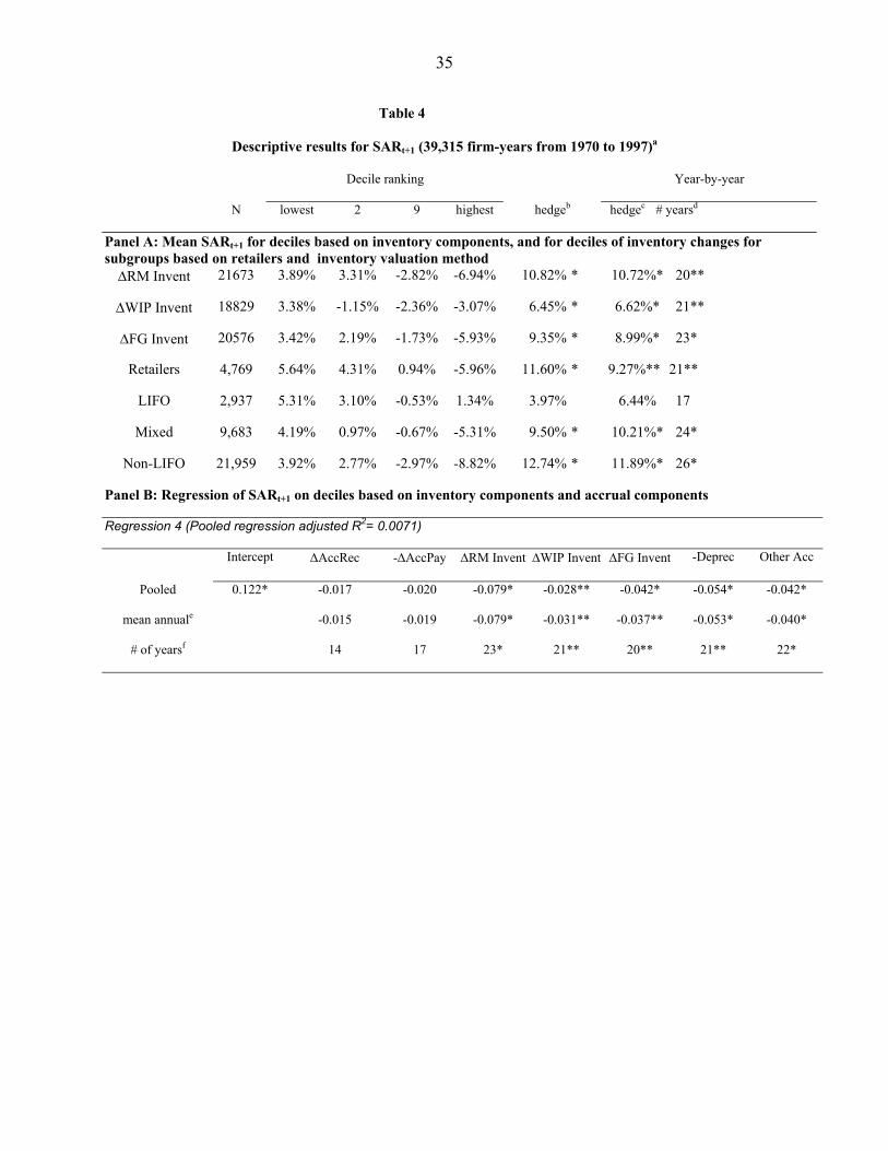
We discuss next some other interesting features of extreme inventory change deciles. To

identify the relative importance of the three components of inventory—RM, WIP and FG—for

the prediction of future abnormal returns, we report in the first three rows of Panel A of Table 4,

the mean abnormal returns earned by deciles formed using changes in each of the three

components. Our results reveal higher hedge returns for changes in RM and FG inventories

(10.82 and 9.35 percent, respectively), which exceed substantially the hedge returns for changes

in WIP inventory (6.45 percent). Note that the sample sizes are reduced considerably when

inventory components are examined, because of missing data.13 To confirm that these findings

13 Since the subsamples used for the three inventory component portfolios are different, and differ also from the

sample for inventory change portfolios, the four sets of results are not strictly comparable. To identify potential differences in these four samples, we computed the inventory change portfolio abnormal returns for each of the three inventory component subsamples. The abnormal returns earned are 10.23 percent, 11.11 percent, and

18

are not due to correlation with other accrual components, we report in Table 4, Panel B, the

results of regression 4, which is obtained by replacing inventory change deciles in regression 2

(see Table 2, Panel B) with deciles of changes in RM, WIP, and FG inventory. The relative

importance of RM inventory changes for future abnormal returns is even more exaggerated in the

regression results.

To provide evidence on the importance of over/underproduction (the effect of varying

production levels on fixed manufacturing overhead per unit absorbed in COGS), we focus on

abnormal returns for inventory deciles for firms in the retail and wholesale industry (SIC

code=5xxx). Since over/underproduction is not relevant for this group, any differences between

the features of this group and those for firms with manufactured inventory could potentially be

attributed to over/underproduction effects. Our results indicate no differences between this

sample and our overall sample. The hedge returns earned by deciles of inventory change for

retailers, reported in the fourth row of Table 4, Panel A, appear similar to those reported in Table

1, Panel A, for the overall sample. We also find that the patterns for seasonally differenced

quarterly COGS/Sales (and SG&A/Sales) resemble substantially the results reported for the

overall sample in Figure 2.

Since inventory changes based on year-end values could reflect unusual inventory

changes that occur in the fourth quarter, we replicated the analysis of mean SARt+1 for inventory

change deciles using seasonal differences for inventory levels as of the first, second, and third

fiscal quarters. We observe levels of hedge returns that are similar to those reported in Table 1,

Panel A, for inventory changes based fourth quarter numbers. These results are inconsistent with

unusual fourth quarter inventory changes being responsible for the observed abnormal returns.

11.37 percent for the RM, WIP, and FG subsamples. As these returns are similar to those observed for the larger sample, we believe meaningful comparisons can be made across all four samples.

19

We also repeated the analysis of seasonally differenced quarterly COGS/Sales and SG&A/Sales,

similar to Figure 2, for extreme inventory change deciles based on second quarter numbers and

observed evidence of unusual patterns, especially for COGS/Sales, around fiscal fourth quarters

before and after the inventory change quarter. These results suggest that there is considerable

overlap among firms represented in the extreme inventory change deciles based on year-end

values and those included in extreme deciles based on interim quarter values.

Our final analysis, relating to a comparison of LIFO and non-LIFO firms, is motivated by

the findings in Hribar (2000) regarding the transparency of the low permanence of earnings

created by LIFO liquidations (inventory decrease firms) and the lower mispricing he observes for

those firms. While LIFO liquidations are highlighted more clearly and thus their income effects

are less likely to be misinterpreted by the stock market, the income effect in year 0 should be

positive for LIFO firms with inventory decreases (since COGS/Sales should decrease when

older, lower inventory costs are expensed), which is contrary to the year 0 income effect noted

for inventory decreases in Figures 1 and 2. Our results, described below, indicate that LIFO firms

with inventory decreases exhibit abnormal returns and COGS/Sales patterns similar to the

patterns observed for other firms with inventory decreases. Quite unexpectedly, LIFO firms with

inventory increases exhibit positive abnormal returns that are markedly different from those for

other firms with inventory increases.

The bottom three rows of Panel A in Table 4 provide the abnormal returns earned in year

+1 by each of the following three groups of firms: a) LIFO firms, that use only the LIFO

valuation method, b) mixed firms, that use LIFO and other valuation methods, and c) non-LIFO

firms, that use methods other than LIFO. While the inventory decrease firms (under the “lowest”

column) exhibit positive abnormal returns that are similar in magnitude across all three groups,

20

the inventory increase firms (under the “highest” column) are clearly different across the three

groups: the non-LIFO group exhibits the most negative abnormal returns and the LIFO group

actually earns positive abnormal returns.

To understand better this unexpected result observed for LIFO firms with inventory

increases, we report in Figure 4 the time series of median COGS/Sales for the LIFO and non-

LIFO partitions of extreme inventory change firms. (The mixed partition exhibits patterns in

between these two partitions, and is deleted from the plot.) The results reported in Figure 4 are

consistent with the abnormal return results reported above. Whereas the two non-LIFO groups

and LIFO firms with inventory decreases exhibit patterns very similar to those presented for our

overall sample (Figure 2, Panel A), LIFO firms with inventory increases exhibit patterns that are

considerably muted: the deviations are generally closer to zero, relative to the other three groups.

5. Conjectures relating to demand shifts and earnings management

Many features of the patterns reported in Figures 1 through 4 are generally inconsistent

with the three explanations considered in section 3, where inventory changes are merely

symptoms of correlated underlying factors that cause profitability changes. The very distinct

profitability patterns (SUE, COGS and SG&A) observed for fourth quarters of years –1 and +1

are not easily reconciled with a one-time shift in reported profitability caused in year 0 by some

other underlying factor. Also, while the profitability changes are positively related to inventory

changes in year 0, the two are inversely related in year –1. Finally, if the results for inventory

changes reflect correlation with omitted underlying factors, why should this correlation be

different for LIFO firms with inventory increases?14 We then considered other possible

14 Other features of our results are also inconsistent with the three explanations. For example, we find evidence

suggesting that the abnormal returns are explained more by the dollar magnitude of inventory changes, rather than percent changes or changes relative to other firms in the same industry (which would be more relevant under those three explanations).

21

explanations and investigated their consistency with our findings. The most promising of those

explanations is one that combines demand shifts with two potential reasons why the stock market

fails to recognize fully the impending reversal in profitability.

The economics and financial statement analysis literatures have long emphasized the

relations among demand shifts, inventory changes, and profitability reversals (e.g., Lev and

Thiagarajan 1993, Abarbanell and Bushee 1997 and 1998). To illustrate the demand explanation,

consider two groups of firms, labeled past winners and past losers, that have experienced demand

and profitability increases and decreases, respectively, over the recent past. Assume that prior

trend is maintained for another year, corresponding to year –1 in our analysis. The stock

market’s reaction is positively related to these demand shifts, and the demand increases

(decreases) in year -1 for past winners (losers) cause a decline (increase) in year-end inventory.

Winners (losers) then anticipate continued growth (declines) in demand into year 0, and increase

(decrease) production in year 0 to satisfy this demand shift and also to compensate for the

inventory declines (increases) in year -1. The subset of these winners (losers) with actual demand

that is less (more) than anticipated demand in year 0 experiences inventory increases (decreases).

In effect, past winners (losers) with extreme demand decreases (increases) in year 0 constitute

our extreme inventory increase (decrease) deciles, and this shift in demand is also associated

with profitability reversals.

In the absence of reliable data on sales that is adjusted for the considerable changes in

entity and scale experienced by extreme inventory change deciles, we are unable to directly

examine the role played by demand shifts. To be sure, some of our results, such as the strong

relation between RM inventory changes and abnormal returns, cannot be reconciled with our

22

demand explanation without imposing additional assumptions and structure.15 Rather than

discuss the details of those assumptions, we focus on why the profitability numbers might not

reflect the reversals until year +1. To recap, while the patterns for inventory levels, profitability,

and abnormal returns for past winners (losers) in year –1 can be reconciled with the increases

(decreases) in demand hypothesized to occur in that year, the continued increases (decreases) in

profitability observed during year 0 are inconsistent with the hypothesized unexpected decreases

(increases) in demand and observed increases (decreases) in inventory. In essence, why are the

profitability reversals predicted for year 0 by our demand shift explanation observed with a lag,

in year +1 reported numbers?

One possibility is that earnings are managed in year 0 to mask these profitability

reversals. While earnings could be managed in a variety of revenue and expense accounts, one

type of earnings management that is unique to inventory balances is related to inventory

“misstatements”. The following cost balance illustrates the impact of inventory misstatement:

COGS equals beginning inventory plus inflows (inventory purchases and manufacturing costs)

less ending inventory. Misstatement of inventory balances is measured relative to inventory

valuations that are observed subsequently. Although it implies bias relative to this ex post value,

misstatement does not imply fraud and any bias is likely to be within the discretion allowed by

GAAP (which is based on reasonable ex ante judgment).16 In essence, overstated (understated)

ending inventory generates understated (overstated) COGS and overstated (understated)

profitability in year 0, and this effect is reversed in year +1.17

15 For example, the RM inventory increases (decreases) for past winners (losers) experiencing unexpected

decreases (increases) in demand could be explained by relatively inflexible contracts with suppliers to purchase RM inventory based on anticipated demand.

16 See evidence in Beasley, Carcello, and Hermanson (1999) for incidence of fraudulent inventory misstatement. 17 Misstatements could be unintentional and due to biased management expectations. For example, in the recent

boom and bust cycle experienced by technology firms, some managers may maintain optimistic expectations of

23

Most of our results for years 0 and +1, including the unusual fourth quarter patterns

observed and the similarity in trends observed for COGS and SG&A, are generally consistent

with the following description: managers of past winners (losers) facing a reversal of

profitability caused by demand shifts in year 0 seek to delay reporting that reversal and maintain

the prior trend by managing earnings upward (downward) in year 0. The incentives for past

winners to defer reporting bad news could arise from a number of sources, including the sharp

disappointment expressed by the market when growth stocks fail to maintain their prior growth

(e.g., Skinner and Sloan 2001). The incentives for past losers to defer reporting good news are

harder to enumerate. Despite some indication that margins for the inventory decrease decile

begin to reflect the profit reversal in the fourth quarter of year 0 (Figure 2, Panel A) and the stock

market partially recognizes this reversal (Figure 1, Panel B), a large fraction of the profitability

reversal and abnormal return occurs in year +1. Perhaps, managers of past losers believe that the

stock market reacts less negatively (than average) to additional bad news, and these negative

accruals are available to boost earnings in future periods.18 Similarly, the absence of abnormal

returns and muted patterns for COGS and SG&A observed for LIFO firms with inventory

increases are not easily explained by earnings management.19

The second reason we consider for delayed recognition of profitability reversals, which

relates to absorption of fixed manufacturing costs, is also unique to inventories. To the extent

that manufacturing costs contain a fixed component that does not vary much with production

inventory valuations even after clear signs of a slowdown in that sector, because of the success they experienced in the past. While the predictions for COGS remain similar to those for the intentional misstatement case, the patterns for SG&A/Sales are not expected to resemble the patterns predicted for COGS/Sales.

18 While these conjectures refer to corporate-level incentives to mislead investors, our evidence is also consistent with earnings management occurring at the divisional level, in response to budgetary incentives.

19 We are unaware of evidence supporting the view that the costs of overstating profits are relatively higher for LIFO firms. To the extent that overstated profits are due to overstated inventory, perhaps LIFO firms avoid adding additional LIFO layers caused by overstated inventory.

24

levels, increases (decreases) in production levels will result in lower (higher) COGS. While this

effect would cause seasonally-differenced COGS/Sales for interim quarters to vary based on

expected production levels for the two fiscal years, seasonally differenced COGS/Sales for the

fourth fiscal quarter is also affected by differences between actual and expected production in

each of the two years (e.g., Jiambalvo, Noreen, and Shevlin 1995). To illustrate, consider the

following description for year –1: past winners (losers) anticipate higher (lower) production

levels in year –1, relative to year –2, and that results in lower (higher) COGS in interim quarters

of year –1. In the fourth quarter of year –1, COGS declines (increases) even further since actual

production was higher (lower) than the original estimates because of the positive (negative)

unexpected demand. In essence, the patterns observed for COGS/Sales in Panel A of Figure 2 are

due to innocent production decisions, and over/under production causes profitability reversals to

be masked in year 0 reported numbers.

While the evidence for COGS/Sales is generally consistent with over/underproduction

some other results suggest that this explanation alone is insufficient. First, we observe similar

quarterly patterns for SG&A, which unlike COGS are not affected by over/underproduction.

Second, we observe similar patterns for our retailer subsample for abnormal returns as well as for

COGS/Sales and SG&A/Sales. Again, over/underproduction is not relevant for these firms. The

different pattern observed only for LIFO firms with inventory increases is also not easily

reconciled with over/underproduction.

Overall, it is feasible that demand shifts cause inventory changes and profit reversals, and

the profit reversals are not clearly revealed to the stock market in reported year 0 profitability

because of earnings management and over/underproduction.

25

6. Conclusions

We find that inventory change is the component of the accrual measure used by Sloan

(1996) that is most strongly related to next year’s abnormal returns. We also find that firms with

inventory increases (decreases) have experienced higher (lower) levels of profitability, growth

and abnormal returns over the prior 5 years, and those trends reverse immediately after the

inventory change. Why inventory changes are related to profitability reversals, and why the stock

market does not recognize the impending profitability shifts are two important questions that we

are unable to provide definitive answers for.

We are, however, able to reject some explanations for our result. We are also able to

document several interesting empirical regularities associated with extreme inventory changes.

Finally, we fashion an explanation that is based on demand shifts, which we hypothesize cause

both the profitability reversals and the inventory changes, and suggest two possible reasons why

the impact of the profitability shift is masked in contemporaneous reported profitability. One

possibility is related to earnings management, potentially by misstating inventory balances, and

the other is related to variation in production levels altering COGS by affecting the amount of

fixed manufacturing overhead absorbed into each unit produced. Inventory changes are related

naturally to demand shifts and both possibilities rely on features unique to inventories. We hope

that the exploratory evidence and demand explanation we offer will serve as a jumping off point

for future research.

26

Appendix

Variable definitions Compustat data item #s are indicated in parentheses next to each item, where appropriate.

Accruals = change in current assets (4) - change in cash (1) - change in current liabilities (5) + change in debt included in current liabilities (34) + change in income taxes payable (71) - depreciation and amortization expense (14), all deflated by average total assets (6). ∆CurLia = change in current liabilities (5) - change in debt included in current liabilities (34) - change in income taxes payable (71), all divided by average total assets (6). (This variable is multiplied by –1 to get the same directional effect as other components of accruals.) ∆CurAss = change in current assets (4) - change in cash (1), scaled by average total assets (6). Deprec = depreciation expense (14) divided by average total assets (6). (This variable is multiplied by –1 to get the same directional effect as other components of accruals.) ∆AccRec = change in accounts receivable (2), deflated by average total assets (6). ∆AccPay = change in accounts payable (70), deflated by average total assets (6). (This variable is multiplied by –1 to get the same directional effect as other components of accruals.) ∆Invent = change in total inventory (3), deflated by average total assets (6). Other Acc = Accruals (as defined above) minus change in accounts receivable (2) plus depreciation and amortization expense (14) minus change in inventory (3) plus change in accounts payable (70) deflated by average total assets ∆RM Invent = change in raw material inventory (76), deflated by average total assets (6). ∆WIP Invent = change in work-in-process inventory (77), deflated by average total assets (6). ∆FG Invent = change in finished goods inventory (78), deflated by average total assets (6). Size adjusted return is computed by taking the raw buy and hold return, inclusive of dividends and subtracting the buy and hold return on a size matched, value-weighted portfolio of firms (obtained from CRSP). The size portfolios are based on market value of equity deciles of NYSE and AMEX firms, as measured at January 1, each year. SARt= ( ) ( )∏∏ +−+

sps

sis rr 11 , where ris and rps are the returns in s for firm i and size portfolio p

For annual periods monthly returns are used, and the portfolio holding periods begin 4 months after the fiscal year-end. For 3-day earnings announcement windows, daily returns are used, and the holding periods are from day –1 to +1 of the earnings announcement date (from Compustat).

27

Growth in Sales = current year’s sales (12) minus previous fiscal year’s sales, divided by previous year’s sales. Capital expenditure = Capital expenditure (30) divided by average total assets (6). ROE = Income before extraordinary items, available for common stocks, (237) divided by ending common equity (60). ROA = Operating income after depreciation (178) divided by average total assets (6). SUE = The seasonal difference in quarterly primary EPS excluding extraordinary items (19), adjusted for stock splits using the Compustat adjustment factor (17), deflated by the closing price as of the third month of the quarter (14). Growth PPE = change in net property, plant and equipment (8) divided by average total assets (6). Growth ONA = change in ONA divided by average total assets (6). ONA is calculated by subtracting working capital (WC) and net PPE (NPPE) from net operating assets (NOA). NOA is defined as (total assets (6) – cash/equivalents (1)) – (total liabilities (181) – long term debt (9) – debt in current liabilities (34)). WC is defined as (current assets (4) – cash/equivalents (1)) – (current liabilities (5) – current debt (34) – taxes payable (71)). NPPE is net property, plant and equipment (8).

28

REFERENCES

Abarbanell, J and B. Bushee. (1998). “Abnormal returns to a fundamental analysis strategy.” The Accounting Review 73, 19-45.

Abarbanell, J and B. Bushee. (1997). “Fundamental analysis, future earnings, and stock prices.” Journal of Accounting Research 35, 1-24.

Ahmed, A.S., K. Nainar, and J. Zhou. (2001). “Do Analysts’ forecasts fully reflect the information in accruals?” Working paper, Syracuse University, Syracuse, NY.

Ali, A., L. Hwang, and M. Twombley. (2000). “Accruals and future stock returns: tests of the naïve investor hypothesis.” Journal of Accounting, Auditing, and Finance, 15, 161-181.

Ball, R., and S. P. Kothari. (1991). “Security returns around earnings announcements.” The Accounting Review 66, 718-739.

Barth, M.E. and A.P. Hutton. (2001). “Financial analysts and the pricing of accruals.” Working paper, Stanford University, Stanford, CA.

Beneish, M.D. and M.E. Vargus. (2001). “Insider Trading, Earnings Quality, and Accrual Mispricing.” Working paper, Indiana University, Bloomington, IN.

Beasley, M.S., J.V. Carcello, and D.H. Hermanson. (1999). “Fraudulent financial reporting: 1987-1997. An analysis of U.S. public companies.” Committee of Sponsoring Organizations of the Treadway Commission (COSO). AICPA (www.aicpa.org).

Bradshaw, M. T., S. A. Richardson, and R.G. Sloan. (2001). “Do analysts and auditors use information in accruals?” Journal of Accounting Research 39, 75-92.

Chan, K., L. Chan, N. Jegadeesh, and J. Lakonishok. (2001). “Earnings Quality and Stock Returns: The Evidence from Accruals.” Working paper, University of Illinois at Urbana-Champaign, IL.

Collins, D. and Hribar, P. (2000). “Earnings-based and accrual-based market anomalies: one effect or two?” Journal of Accounting and Economics 29, 101-124.

Collins, D. and Hribar, P. (2002). “Errors in estimating accruals: implications for empirical research.” Journal of Accounting Research. 40 (forthcoming).

Fairfield, P.M., J.S. Whisenant, and T.L. Yohn. (2001). “Accrued earnings and growth: implications for earnings persistence and market mispricing.” Working paper, Georgetown University, Washington, D.C.

Hribar, P. (2000). “The market pricing of components of accruals.” Working paper, Cornell University, Ithaca, NY.

Jiambalvo, J., E. Noreen, and T. Shevlin. (1995). “Incremental information content of the change in the percent of production added to inventory.” Working paper, University of Washington, Seattle, WA.

Lev, B. and R. Thiagarajan. (1993). “Fundamental information analysis.” Journal of Accounting Research 31, 190-215.

29

Mishkin, F., (1983). A rational expectations approach to macroeconomics. The University of Chicago Press, Chicago, IL.

Richardson, S. and I. Tuna. (2001). “Earnings quality: Sloan (1996) revisited.” Working Paper, University of Michigan, Ann Arbor, MI.

Richardson, S.A., R.G. Sloan, M.A. Soliman, and I.Tuna. (2001). “Information in accruals about the quality of earnings.” Working paper, University of Michigan, Ann Arbor, MI.

Sloan, R.G. (1996). “Do stock prices fully reflect information in accruals and cash flows about future earnings?” The Accounting Review 71, 289-315.

Skinner D. and R. Sloan. (2001). “Don’t let earnings torpedo sink your portfolios.” Working Paper, University of Michigan, Ann Arbor, MI.

Tarpley, R.L. (2000). “Profitability of information contained in the accrual component of earnings.” Working paper, Cornell University, Ithaca, NY.

Titman, S., K.C.J. Wei, and F. Xie. (2001). “Capital investments and stock returns.” Working paper, University of Texas at Austin, Austin, TX.

Xie, H. (2001). “The mispricing of abnormal accruals.” The Accounting Review 76, 357-374.

Zach, T. (2001). “Inside the ‘Accrual Anomaly’: a closer look at methodological issues.” Working paper, University of Rochester, Rochester, NY.

30

Table 1

Analysis of accrual components (39315 firm-years from 1970 to 1997)a

Decile ranking Year-by-year

N lowest 2 9 highest hedgeb hedgec # yearsd

Panel A: SARt+1 for deciles of accruals and its components

Accruals 39315 3.30% 2.25% -2.91% -5.98% 9.28% * 8.84%* 22*

∆CurAss 39315 3.23% 1.80% -2.74% -5.86% 9.09% * 8.82%* 23*

-∆CurLia 39315 0.35% 0.45% -0.86% -0.99% 1.34% 1.27% 17

-Deprec 39315 1.05% 1.18% -1.23% -3.69% 4.74% * 4.43%** 18

∆AccRec 39315 0.69% 0.53% -1.81% -2.97% 3.67% * 3.62%** 18

-∆AccPay 39315 -2.09% -0.33% 1.26% 0.65% -2.74% ** -2.64% 13

∆Invent 39315 4.50% 1.81% -1.52% -6.89% 11.39% * 11.05%* 27*

Other Acc 39315 2.41% 0.12% -1.11% -1.37% 3.78% * 3.74%* 22*

Panel B: Regression of SARt+1 on deciles of accrual components

Regression 1 (Pooled regression adjusted R2= 0.0034) Intercept ∆CurAss -∆CurLia -Deprec

Pooled 0.077* -0.083* -0.035* -0.035*

mean annuale -0.080* -0.035* -0.032**

# of yearsf 23* 19 20**

Regression 2 (Pooled regression adjusted R2= 0.0042) Intercept ∆AccRec -∆AccPay ∆Invent -Deprec Other Acc

Pooled 0.081* -0.016** -0.006 -0.075* -0.034* -0.043*

mean annual -0.017 -0.007 -0.071* -0.032** -0.042*

# of years 19 16 23* 20** 22*

31

Notes:

a. The variables are calculated as indicated below (see appendix for details) and all regressors are sorted into deciles and assigned

values between 0 and 1. All changes are scaled by average total assets, unless indicated otherwise.

SARt+1=12-month buy and hold return beginning 4 months after fiscal year-end of inventory change year less corresponding size

portfolio buy and hold return.

Accruals = the change in non-cash current assets, less the change in current liabilities (exclusive of short-term debt and taxes

payable), less depreciation expense.

∆CurAss = change in non-cash current assets

-∆CurLia = minus change in current liabilities (exclusive of short-term debt and taxes payable)

-Deprec = minus depreciation and amortization expense

∆AccRec = change in accounts receivable

-∆AccPay = minus change in accounts payable

∆Invent = change in total inventory

Other Acc = accruals minus change in accounts receivable and inventory plus change in accounts payable plus depreciation and

amortization expense

b. Hedge is the difference in size-adjusted return between the lowest and highest decile.

c. Mean hedge reports the mean value of annual hedge portfolio returns. Statistical significance is based on a t-test using

magnitudes of the 28 annual hedge returns.

d. # of years reports the number of years in which the hedge portfolio return is positive. Statistical significance is based on a sign

test using signs of the 28 annual hedge returns.

e. Mean annual reports the mean value of annual coefficient estimates. Statistical significance is based on a t-test using

magnitudes of the 28 annual coefficient estimates.

f. # of years reports the number of years in which the coefficient is negative. Statistical significance is based on a sign test using

signs of the 28 annual coefficient estimates.

*: significant at the 1% level;

**:significant at the 5% level;

32

Table 2

Analysis of three explanations: (39,315 firm-years from 1970 to 1997)a



Panel A: Mean SARt+1 for deciles of growth in PPE and ONA

Growth PPE 39290 3.11% 3.10% -0.58% -4.56% 7.67% * 7.46%* 23*

Growth ONA 39253 2.30% 2.11% -2.08% -3.75% 6.05% * 6.03%* 24*

Panel B: Multivariate regression SARt+1 on accrual components and deciles of growth in PPE and ONA

Regression 3 (Pooled regression adjusted R2= 0.0071) Intercept ∆AccRec -∆AccPay ∆Invent -Deprec Other Acc Growth PPE Growth ONA

Pooled 0.126* -0.01 -0.014*** -0.061* -0.037* -0.045* -0.057* -0.057*

mean annuale -0.011 -0.017 -0.057* -0.036** -0.044* -0.059* -0.058*

# of yearsf 15 17 22* 18 22* 23* 25*

33

Notes:




decile buy and hold return.

Growth PPE = change in net property, plant and equipment.

Growth ONA = change in other (net) long-term assets and non-interest bearing liabilities.

Accruals = the change in non-cash current assets, less the change in current liabilities (exclusive of short-term debt and taxes

payable), less depreciation expense.




∆Invent = change in total inventory












*: significant at the 1% level.

**: significant at the 5% level..

34

Table 3

Time-series of key financial variables around the year with extreme inventory changes

Year relative to year 0, the year with the extreme inventory change

-5 -4 -3 -2 -1 0 1 2 Next year’s size adjusted return (SARt+1), over the 12 months beginning 4 months after the fiscal year end

lowest -6.72% -17.11% -9.44% -4.19% -4.32% 4.50% 1.47% 1.86%

highest 3.05% 13.08% 9.60% 6.39% 3.82% -6.89% -1.66% -0.36%

median growth in sales

lowest 9.85% 9.22% 9.58% 8.02% 5.31% -3.68% 2.76% 6.92%

highest 11.99% 12.49% 12.68% 13.50% 14.87% 18.52% 15.02% 9.64%

median capital expenditure

lowest 5.26% 5.18% 5.10% 4.91% 4.60% 3.81% 3.99% 4.39%

highest 5.42% 5.42% 5.25% 5.42% 5.59% 6.37% 5.52% 5.07%

median ROE

lowest 10.39% 10.02% 9.54% 8.61% 6.69% 5.02% 8.04% 9.06%

highest 12.41% 12.52% 12.61% 12.92% 13.37% 13.11% 11.50% 11.16%

median ROA

lowest 10.17% 9.73% 9.33% 8.47% 6.92% 5.63% 7.34% 8.02%

highest 12.57% 12.64% 12.71% 12.88% 13.37% 13.05% 11.40% 10.84%

Notes:

SARt+1 = 12-month buy and hold return, beginning 4 months after the fiscal year-end, in excess of the corresponding size decile

buy and hold returns

Lowest= lowest decile of inventory change

Highest= highest decile of inventory change

Growth in Sales = Percent change in sales.

Capital expenditure = Capital expenditures divided by average total assets

ROE = Income before extraordinary items- available for common stocks divided by book value of common equity

ROA = Operating income after depreciation divided by average total assets.

35

Table 4

Descriptive results for SARt+1 (39,315 firm-years from 1970 to 1997)a



Panel A: Mean SARt+1 for deciles based on inventory components, and for deciles of inventory changes for subgroups based on retailers and inventory valuation method

∆RM Invent 21673 3.89% 3.31% -2.82% -6.94% 10.82% * 10.72%* 20**

∆WIP Invent 18829 3.38% -1.15% -2.36% -3.07% 6.45% * 6.62%* 21**

∆FG Invent 20576 3.42% 2.19% -1.73% -5.93% 9.35% * 8.99%* 23*

Retailers 4,769 5.64% 4.31% 0.94% -5.96% 11.60% * 9.27%** 21**

LIFO 2,937 5.31% 3.10% -0.53% 1.34% 3.97% 6.44% 17

Mixed 9,683 4.19% 0.97% -0.67% -5.31% 9.50% * 10.21%* 24*

Non-LIFO 21,959 3.92% 2.77% -2.97% -8.82% 12.74% * 11.89%* 26*

Panel B: Regression of SARt+1 on deciles based on inventory components and accrual components

Regression 4 (Pooled regression adjusted R2= 0.0071)

Intercept ∆AccRec -∆AccPay ∆RM Invent ∆WIP Invent ∆FG Invent -Deprec Other Acc

Pooled 0.122* -0.017 -0.020 -0.079* -0.028** -0.042* -0.054* -0.042*

mean annuale -0.015 -0.019 -0.079* -0.031** -0.037** -0.053* -0.040*

# of yearsf 14 17 23* 21** 20** 21** 22*

36

Notes:




portfolio buy and hold return.






Retailers includes all firms in the 5xxx SIC industry group (expected to have no manufacturing costs)

∆RM Invent = change in raw material inventory

∆WIP Invent = change in work-in-process inventory

∆FG Invent = change in finished goods inventory

Inventory method is coded as LIFO if the LIFO method alone is used, as non-LIFO if the LIFO method is not used, and as mixed

for all other firm-years.










*: significant at the 1% level;

**:significant at the 5% level;

37

Figure 1 Time-series of quarterly unexpected earnings and abnormal returns for extreme inventory change deciles

Panel A: Mean seasonally-differenced quarterly eps, scaled by price (Winsorized at –1 and +1)

Panel B: Mean size-adjusted returns for 3-day earnings announcement windows.

-3.00%

-2.00%

-1.00%

0.00%

1.00%

2.00%

3.00%

4.00%

-7 -6 -5 -4 -3 -2 -1 0 1 2 3 4 5 6 7 8

quarter relative to 4th quarter of year 0

Seas

onal

ly d

iffer

ence

d qu

arte

rly e

arni

ngs,

sca

led

by p

rice

extreme inventory decreases

extreme inventory increases

-1.00%

-0.50%

0.00%

0.50%

1.00%

1.50%

-7 -6 -5 -4 -3 -2 -1 0 1 2 3 4 5 6 7 8

quarter relative to 4th quarter of year 0

Size

-adj

uste

d re

turn



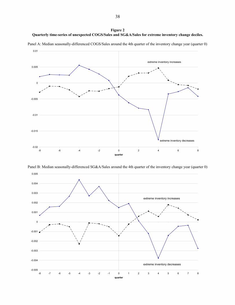
38

Figure 2 Quarterly time-series of unexpected COGS/Sales and SG&A/Sales for extreme inventory change deciles.

Panel A: Median seasonally-differenced COGS/Sales around the 4th quarter of the inventory change year (quarter 0)

Panel B: Median seasonally-differenced SG&A/Sales around the 4th quarter of the inventory change year (quarter 0)

-0.005

-0.004

-0.003

-0.002

-0.001

0

0.001

0.002

0.003

0.004

0.005

-8 -7 -6 -5 -4 -3 -2 -1 0 1 2 3 4 5 6 7 8

quarter



-0.02

-0.015

-0.01

-0.005

0

0.005

0.01

-8 -6 -4 -2 0 2 4 6 8

quarter



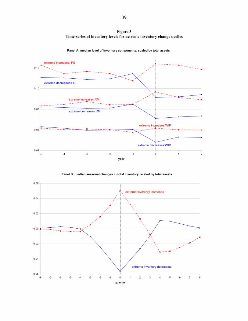
39

Figure 3 Time-series of inventory levels for extreme inventory change deciles

0.04

0.06

0.08

0.10

0.12

-5 -4 -3 -2 -1 0 1 2

year

extreme increases:RM

extreme decreases:RM

extreme increases:WIP

extreme decreases:WIP

extreme increases: FG

extreme decreases:FG

Panel A: median level of inventory components, scaled by total assets

Panel B: median seasonal changes in total inventory, scaled by total assets

-0.06

-0.04

-0.02

0.00

0.02

0.04

0.06

-8 -7 -6 -5 -4 -3 -2 -1 0 1 2 3 4 5 6 7 8

quarter



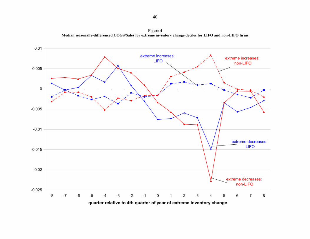
40

Figure 4 Median seasonally-differenced COGS/Sales for extreme inventory change deciles for LIFO and non-LIFO firms

-0.025

-0.02

-0.015

-0.01

-0.005

0

0.005

0.01

-8 -7 -6 -5 -4 -3 -2 -1 0 1 2 3 4 5 6 7 8

quarter relative to 4th quarter of year of extreme inventory change

extreme decreases: non-LIFO

extreme increases: LIFO

extreme increases: non-LIFO

extreme decreases: LIFO

Inventory changes and future returns - Faculty...

Documents

Transcript of Inventory changes and future returns - Faculty...