Comovement - Faculty Directoryfaculty.som.yale.edu/nicholasbarberis/sap_jnl.pdf ·...

ARTICLE IN PRESS

Journal of Financial Economics 75 (2005) 283–317

0304-405X/$

doi:10.1016/j

$We than

Kaplan, Ant

anonymous

School of Ec

University of

helpful comm

assistance, th

providing da�CorrespoE-mail ad

www.elsevier.com/locate/econbase

Comovement$

Nicholas Barberisa, Andrei Shleiferb,�, Jeffrey Wurglerc

aYale School of Management, New Haven, CT 06520, USAbDepartment of Economics, Littauer Center, Harvard University, Cambridge, MA 02138, USA

cNYU Stern School of Business, New York, NY 10012, USA

Accepted 1 April 2004

Available online 25 September 2004

Abstract

Building on Vijh (Rev. Financial Stud. 7 (1994)), we use additions to the S&P 500 to

distinguish two views of return comovement: the traditional view, which attributes it to

comovement in news about fundamental value, and an alternative view, in which frictions or

sentiment delink it from fundamentals. After inclusion, a stock’s beta with the S&P goes up. In

bivariate regressions which control for the return of non-S&P stocks, the increase in S&P beta

is even larger. These results are generally stronger in more recent data. Our findings cannot

easily be explained by the fundamentals-based view and provide new evidence in support of

the alternative friction- or sentiment-based view.

r 2004 Elsevier B.V. All rights reserved.

JEL classification: G12

Keywords: Comovement; Beta; Index inclusion

- see front matter r 2004 Elsevier B.V. All rights reserved.

.jfineco.2004.04.003

k John Campbell, Ned Elton, Kenneth French, Will Goetzmann, Joel Hasbrouck, Steven

hony Lynch, Mike Ryngaert, Bill Schwert, Robert Shiller, Tuomo Vuolteenaho, two

referees, seminar participants at Columbia University, Harvard University, the London

onomics, New York University, Rice University, UCLA, the University of Chicago, the

Florida at Gainesville, the University of Notre Dame, Yale University and the NBER for

ents, Huafeng Chen and Bill Zhang for helpful comments and outstanding research

e Q Group for financial support, and Rick Mendenhall and Standard and Poor’s for

ta.

nding author. Tel.: +1-617-495-5046; fax: +1-617-496-1708.

dress: [email protected] (A. Shleifer).

www.elsevier.com/locate/econbase

ARTICLE IN PRESS

N. Barberis et al. / Journal of Financial Economics 75 (2005) 283–317284

1. Introduction

Researchers have uncovered numerous patterns of comovement in asset returns.There are strong common factors in the returns of small-cap stocks, value stocks,closed-end funds, stocks in the same industry, and bonds of the same rating andmaturity. There is common movement of individual stocks within national marketsand also among international markets themselves.A substantial body of work examines whether the sensitivity of asset returns to

common factors such as these can help explain average rates of return. Much lesswork, however, has been done to understand why common factors arise in the firstplace. Why do certain groups of assets comove while others do not? What determinesassets’ betas on these common factors? In this paper, we consider two broad theoriesof comovement—one traditional, the other more novel—and present new evidenceto distinguish between them.The traditional theory, derived from economies without frictions and with rational

investors, holds that comovement in prices reflects comovement in fundamental values.In a frictionless economy with rational investors, price equals fundamental value—anasset’s rationally forecasted cash flows discounted at a rate appropriate for their risk—and so any comovement in prices must be due to comovement in fundamentals.In economies with frictions or with irrational investors, and in which there are

limits to arbitrage, comovement in prices is delinked from comovement infundamentals. This suggests a second broad class of ‘‘friction-based’’ and‘‘sentiment-based’’ theories of comovement. We examine three specific views ofcomovement that can be described in these terms.The first is the category view, analyzed by Barberis and Shleifer (2003). They argue

that, to simplify portfolio decisions, many investors first group assets into categoriessuch as small-cap stocks, oil industry stocks, or junk bonds, and then allocate fundsat the level of these categories rather than at the individual asset level. If some of theinvestors using categories are noise traders with correlated sentiment, and if theirtrading affects prices, then as they move funds from one category to another, theircoordinated demand induces common factors in the returns of assets that happen tobe classified into the same category, even when these assets’ cash flows areuncorrelated.1

Another kind of comovement, which we refer to as the habitat view, starts fromthe observation that many investors choose to trade only a subset of all availablesecurities. Such preferred habitats could arise because of transaction costs,international trading restrictions, or lack of information. As these investors’ riskaversion, sentiment, or liquidity needs change, they alter their exposure to thesecurities in their habitat, thereby inducing a common factor in the returns of thesesecurities. This view of comovement predicts that there will be a common factor inthe returns of securities that are held and traded by a specific subset of investors,such as individual investors.

1Mullainathan (2002) provides a more general analysis of the use of categories for processing

information.

ARTICLE IN PRESS

N. Barberis et al. / Journal of Financial Economics 75 (2005) 283–317 285

A third view of comovement, the information diffusion view, holds that, due tosome market friction, information is incorporated more quickly into the prices ofsome stocks than others. For example, some stocks may be less costly to trade, ormay be held by investors with faster access to breaking news and the resourcesrequired to exploit it. In this view, there will be a common factor in the returns ofstocks that incorporate information at similar rates: when good news aboutaggregate earnings is released, some stocks reflect it today and move up togetherimmediately; the remaining stocks also move up together, but only after some delay.2

Early evidence of friction- or sentiment-based comovement can be found in Vijh(1994), who studies changes in the market betas of stocks added to the S&P 500index. Standard & Poor’s emphasizes that in choosing stocks for inclusion in theS&P 500, they are simply trying to make their index as representative as possible ofthe overall U.S. economy, not signaling an opinion about fundamental value. If so,inclusion should not change investors’ perception of the correlation of the includedstock’s fundamental value with other stocks’ fundamental values. Under thetraditional view of comovement, then, inclusion should not change the correlation ofthe included stock’s return with the returns of other stocks.The friction- or sentiment-based views make a different prediction. Consider first

the category and habitat views. The vast popularity of S&P-linked investmentproducts, such as S&P mutual funds, futures, and options, suggests that the index isa preferred habitat for some investors and a natural category for many more. Whena stock is added to the S&P, it enters a category (habitat) used by many investors andis buffeted by fund flows in and out of that category (habitat). If arbitrage is limited,these fund flows raise the correlation of the included stock’s return with the returnsof other stocks in the S&P.The information diffusion view also predicts a rise in the correlation of the added

stock’s return with the S&P return. Under this view, stocks in the S&P 500 are quickto incorporate news about aggregate cash flows, perhaps because they haveparticularly low trading costs or are held by investors with better access to news.When a stock enters the S&P, it starts to incorporate market-wide news at the sametime as other S&P stocks, rather than, say, a day later. As a result, it comoves morewith other S&P stocks after inclusion than before.In fact, Vijh (1994) finds that at both daily and weekly frequencies, stocks added to

the index between 1975 and 1989 experience a significant increase in their betas onthe value-weighted return of NYSE and AMEX stocks, a close proxy for the value-weighted S&P return. In contrast to the fundamentals view, but consistent with thethree friction- or sentiment-based views, addition to the index leads to a shift in thecorrelation structure of returns.3

2A related view, that makes similar predictions, is that it is market-wide sentiment and not just market-

wide cash-flow news that is incorporated more quickly into some stocks than others. In this view, there will

be a common factor in the returns of stocks that incorporate sentiment at similar rates.3Vijh (1994) computes betas with the overall market return rather than with the S&P return because his

main objective is to understand whether investor trading patterns affect the standard measure of asset

risk—market beta—and not to design the most powerful test of friction- or sentiment-based comovement.

ARTICLE IN PRESS


In this paper, we return to additions to the S&P 500 and provide new evidence insupport of the friction- or sentiment-based theories of comovement. First, byapplying a univariate regression analysis similar to Vijh’s to the longer sample ofdata now available, we uncover considerably larger effects. While stocks added tothe S&P during 1976–1987 experience an average increase in daily S&P beta of 0.067after inclusion, the average increase in the 1988–2000 period is 0.214. In light of thegrowing importance of the S&P 500 as both a category and a habitat, the fact thatthe effect is not only present but larger in more recent data is especially supportive ofthe friction- or sentiment-based views.Our second and principal contribution is to introduce a bivariate regression test to

distinguish between the two broad theories of comovement. The friction- orsentiment-based views imply that, in a bivariate regression of a stock’s return onboth the S&P and a non-S&P ‘‘rest of the market’’ index, the S&P beta should go upafter inclusion while the non-S&P beta should fall; that these patterns should go inthe opposite direction for stocks deleted from the index; and that they should bestronger in more recent data. The fundamentals view, in contrast, predicts no shift inS&P and non-S&P betas after inclusion.The bivariate regressions provide evidence of friction- or sentiment-based

comovement altogether stronger than that uncovered by the univariate tests. Atdaily, weekly, and even monthly frequencies, the bivariate tests show a strikingincrease in S&P betas and decline in non-S&P betas. At the daily frequency, forexample, S&P betas increase by 0.326 on average over the 1976–2000 period, whilenon-S&P betas fall by an average of 0.319. Significant results in the oppositedirection are observed when stocks are deleted from the index, and the effects arequantitatively larger in more recent data.We examine the robustness of these findings in several ways. We obtain similar

results when analyzing the data from a ‘‘calendar time’’ rather than an ‘‘eventtime’’ perspective. We also find that the results cannot be attributed to thintrading. Finally, we show that the shifts in S&P betas for stocks added to the indexare much larger than those for a sample of ‘‘matched’’ stocks, namely stocks similarto the event stocks in a number of characteristics, but which are not included in theindex. This last observation rules out certain fundamentals-based explanations ofour results under which inclusion in the S&P coincides with a change in thecorrelations between stocks’ fundamental values, even if it does not cause such achange.While our results are consistent with all three variants of friction- or sentiment-

based comovement—category, habitat, and information diffusion—we also attemptto determine how big a role each of them plays. In particular, we decompose the shiftin betas around inclusion into a component due to information diffusion and aresidual component, more likely due to category and habitat effects. Theinformation diffusion story has the distinguishing feature that it predicts nonzerocross-autocorrelations between S&P and non-S&P returns. We can therefore identifyits effect by including lead and lag terms in the regressions. Our analysis suggeststhat a small fraction of the daily univariate results and a much larger fraction of thedaily bivariate results are due to information diffusion effects.

ARTICLE IN PRESS


Our paper adds to a growing body of evidence that can be naturally understood asfriction- or sentiment-based comovement. Froot and Dabora (1999) show that thereturns of Royal Dutch shares are surprisingly delinked from the returns of Shellshares, even though the two stocks are claims to the same cash-flow stream andtherefore have the same fundamental value. Hardouvelis et al. (1994) and Bodurthaet al. (1995) show that closed-end country funds comove as much with the stockmarket in the country where they are traded as with the stock market in the countrywhere their assets are traded. Lee et al. (1991) find that domestic closed-end fundsoften comove with small-cap stocks even when their asset holdings consist of large-cap stocks. Pindyck and Rotemberg (1990) uncover evidence of excess comovementin the prices of seven major commodities. Fama and French (1995) show that it ishard to connect the strong common factors in the returns of value stocks and smallstocks to common factors in news about earnings.4

Greenwood and Sosner (2002) test the friction- or sentiment-based views usingdata on additions to and deletions from the Nikkei 225 index. They find increases inbeta and R2 following addition to the index, and decreases following deletions. Theirevidence is therefore also consistent with our predictions; if anything, the results forthe Japanese data are even stronger than those for the U.S. data.A large literature examines whether index inclusion has a contemporaneous effect

on price levels. Harris and Gurel (1986), Shleifer (1986), Lynch and Mendenhall(1997), and Wurgler and Zhuravskaya (2002) find strong price effects for S&P 500inclusions, while Kaul et al. (2000) and Greenwood (2004) find similar effects in theToronto Stock Exchange TSE 300 and Nikkei 225 indices, respectively. Thisliterature argues that uninformed demand affects price levels; our paper shows that itmay also affect patterns of comovement.5

In Section 2, we present the basic predictions of the three friction- or sentiment-based views of comovement. In Section 3, we test these predictions using data onS&P 500 inclusions and deletions. Section 4 concludes.

2. Theories of comovement

The traditional theory of return comovement is the fundamentals-based view,under which the returns of two assets are correlated because changes in the assets’

4Fundamentals-based comovement can be generated through news about discount rates, as well as

through news about earnings. However, changes in interest rates or risk aversion induce a common factor

in the returns on all stocks, and do not explain why a particular subset of stocks comove. A common

factor in news about the risk of certain assets could, in principle, be a source of comovement for those

assets, but there is little evidence to support such a mechanism in the case of small stocks or value stocks.5Numerous other papers also present evidence consistent with uninformed demand affecting prices.

These include French and Roll (1986), Cooper et al. (2001), Gompers and Metrick (2001), Mitchell et al.

(2002), Goetzmann and Massa (2003), and Lamont and Thaler (2003). Cooper et al. (2001) is particularly

related to the category view in that they show that stocks that recategorized themselves as dot-com

companies in the late 1990s experienced large price increases even when their business model did not

change.

ARTICLE IN PRESS


fundamental values are correlated. In this section, we briefly present reduced-formmodels of three alternative friction- or sentiment-based theories of comovement: thecategory, habitat, and information diffusion views. The models yield the predictionsthat motivate the empirical work in Section 3.Consider an economy that contains a riskless asset in perfectly elastic supply and

with zero rate of return, and also 2n risky assets in fixed supply. Risky asset i is aclaim to a single liquidating dividend Di;T to be paid at some later time T. Thiseventual dividend equals

Di;T ¼ Di;0 þ ei;1 þ � � � þ ei;T ; ð1Þ

where Di;0 and ei;t are announced at time 0 and time t, respectively, and where

et ¼ ðe1;t; . . . ; e2n;tÞ0� Nð0;SDÞ; i:i:d: over time: ð2Þ

The price of a share of risky asset i at time t is Pi;t and the return on the asset betweentime t � 1 and time t is

DPi;t Pi;t � Pi;t�1: ð3Þ

For simplicity, we refer to the asset’s change in price as its return.Suppose that, to simplify their decision-making, some investors group the 2n risky

assets into two categories, X and Y, and then allocate funds at the level of thesecategories rather than at the individual asset level. In particular, they place assets 1through n in category X and assets n þ 1 through 2n in category Y. It may be helpfulto think of X and Y as ‘‘old economy’’ and ‘‘new economy’’ stocks, respectively.Suppose now that these categories are also adopted by noise traders, who channel

funds in and out of the categories depending on their sentiment. A simplerepresentation for asset returns is then

DPi;t ¼ ei;t þ DuX ;t; i 2 X ; ð4Þ

DPj;t ¼ ej;t þ DuY ;t; j 2 Y ; ð5Þ

where

uX ;t

uY ;t

� �� N

0

0

� �;s2u

1 ru

ru 1

� �� ; i:i:d: over time: ð6Þ

Here, uX ;t can be thought of as time t noise trader sentiment about the securities incategory X. Since the noise traders allocate funds by category, this sentiment level isthe same for all securities in category X. Eq. (4) says that the return on a security incategory X is affected not only by news about cash flows, ei;t, but also by the changein sentiment about X, DuX ;t: when noise traders become more bullish about oldeconomy stocks, these stocks go up in price.Eqs. (4) and (5) can also be thought of as a reduced-form model for the habitat

view of comovement. In this case, X and Y simply have to be reinterpreted ashabitats, not categories: instead of representing groups of assets that some investorsdo not distinguish between when allocating funds, they represent groups of assetsthat are the sole holdings of some investors. Specifically, we can think of assets 1through n as U.S. stocks and assets n þ 1 through 2n as U.K. stocks; there are many

ARTICLE IN PRESS


investors in both countries who trade only domestic securities. Under the habitatinterpretation, uX ;t tracks the risk aversion, sentiment, or liquidity needs of investorswho invest only in the securities in X. The return of an asset in habitat X is affectednot only by news about cash flows but also by the change in risk aversion, say, ofthese specific investors.The third variant of friction- or sentiment-based comovement, the information

diffusion view, can be modeled as

DPi;t ¼ ei;t; i 2 X ; ð7Þ

DPj;t ¼ mej;t þ ð1� mÞej;t�1; j 2 Y : ð8Þ

Here, X and Y are groups of stocks that, for some reason, incorporate newinformation at different rates. Stocks in X incorporate news announced at time t

immediately. Stocks in Y incorporate only a fraction m of time t news immediately;the remaining fraction, 1� m, is incorporated in the following period.For the fund flows of noise traders or investors with preferred habitats to affect

prices, as in Eqs. (4)–(5), or for information to be incorporated into stock prices withdelay, as in Eqs. (7)–(8), arbitrage must be limited in some way, perhaps becausearbitrageurs have short horizons (De Long et al., 1990; Shleifer and Vishny, 1997).The idea that there are limits to arbitrage has found support in the considerableempirical literature, cited in the introduction, suggesting that demand unrelated tonews about fundamental value affects security prices.6

To uncover evidence of friction- or sentiment-based comovement, we look fortestable predictions that emerge from our reduced-form models. One set ofpredictions describes what happens when a stock moves from one category orhabitat to another, or from a group of stocks that incorporates information slowly toone that does so quickly. Such reclassification occurs in many ways. For example, ifthe market capitalization of a large-cap stock declines sufficiently, it enters the small-cap stock category. More simply, stocks are regularly added to categories like theS&P 500 to replace stocks that have been removed due to bankruptcies or mergers.In the appendix, we show that under quite general conditions, the reduced-form

models (4)–(5) and (7)–(8) yield the following prediction:

Prediction 1. Suppose that risky asset j, previously a member of Y, is reclassified into

X, and that the cash-flow covariance matrix SD is constant over time. Then, for a large

number of risky assets n, the probability limit of the OLS estimate of bj in the

univariate regression

DPj;t ¼ aj þ bjDPX ;t þ vj;t; ð9Þ

6Barberis et al. (2002) show more formally that in an economy where rational arbitrageurs interact

either with category-based noise traders or with investors with preferred habitats, returns have the form

given in Eqs. (4)–(5).

ARTICLE IN PRESS


where

DPX ;t ¼1

n

Xl2X

DPl;t; ð10Þ

as well as the probability limit of the R2 of this regression, increases after

reclassification.

The intuition is straightforward, whether X and Y are categories, habitats, orgroups of stocks that incorporate information at similar rates. To take the categoryview, when asset j enters category X, it is buffeted by noise traders’ flows of funds inand out of that category. This increases the covariance of its return with the returnon category X, DPX ;t, and hence also its beta loading on that return. For simplicity,we assume a fixed cash-flow covariance matrix in the statement of the prediction. Amore general version would predict that beta increases more than can be explainedby any change in cash-flow correlations.A similar intuition lies behind the next prediction which, as we show in the

Appendix, can also be derived from Eqs. (4)–(5) and (7)–(8):

Prediction 2. Suppose that risky asset j, previously a member of Y, is reclassified into

X, and that the cash-flow covariance matrix SD is constant over time. Then, for a large

number of risky assets n, the probability limit of the OLS estimate of bj;X in the

bivariate regression

DPj;t ¼ aj þ bj;XDPX ;t þ bj;YDPY ;t þ vj;t ð11Þ

rises after reclassification, while the probability limit of the OLS estimate of bj;Y falls.

In particular, the pre-reclassification values of the two slope coefficients, bj;X

and bj;Y,

and their post-reclassification values, bj;X and bj;Y , satisfy

bj;X

¼ 0; bj;Y

¼ 1

0obj;X o1; 0obj;Yo1; bj;X þ bj;Y ¼ 1:

The intuition for this prediction is again straightforward, whichever interpretationX and Y are given. Consider again the category view, whose basic prediction is that,when a stock enters category X, it becomes more sensitive to the category X

sentiment shock DuX ;t. The independent variable in the Prediction 1 regression,DPX ;t, is not a clean measure of this sentiment shock: as Eq. (4) shows, a substantialpart of its variation comes from news about cash flows. The DPY ;t variable inregression (11) can be thought of as a control for such news, making the coefficienton DPX ;t a cleaner measure of sensitivity to DuX ;t. Alternatively, under theinformation diffusion view, regression (11) is a cleaner test than regression (9) ofwhether, after inclusion, stock j becomes more sensitive to that component ofmarket-wide news that is incorporated more quickly into X than into Y. Note thatwhile bj;X rises after reclassification, it rises by less than one, and that while bj;Y falls,

ARTICLE IN PRESS


it falls by less than one. Moreover, the rise in bj;X has the same absolute magnitudeas the fall in bj;Y .Later on, when we try to distinguish not only between the fundamentals-based and

the friction- or sentiment-based theories of comovement, but also between the threespecific variants of friction- or sentiment-based comovement, we make use of aprediction of the information diffusion view not shared by the category and habitatviews, namely that there will be positive cross-autocorrelation between S&P andnon-S&P returns. Under the information diffusion view, news about aggregatecash flows is reflected in S&P stocks today, but only with some delay in non-S&Pstocks.The three friction- or sentiment-based views we consider depend on the existence

of noise traders who allocate funds by category, on the existence of distinct investorhabitats, or on heterogeneous rates of information diffusion. If these features are notpresent, Predictions 1 and 2 will not hold. In this case,

DPi;t ¼ ei;t; i 2 X ð12Þ

DPj;t ¼ ej;t; j 2 Y ; ð13Þ

and comovement is entirely fundamentals-based, in that the correlation of returns iscompletely determined by the correlation of cash-flow news. If, as assumed in thepredictions, the cash-flow covariance matrix SD remains constant, the correlationstructure of returns also remains constant. In other words, bj and R2 in Prediction 1and bj;X and bj;Y in Prediction 2 remain unchanged after reclassification.

3. Empirical tests

To test Predictions 1 and 2, we need a group of securities with three characteristics.First, the group must be a natural category or preferred habitat for manyinvestors, or else a set of stocks that incorporate information more quicklythan do other stocks. Second, since the predictions concern reclassification,there must be clear and identifiable changes in group membership. Finally, tocontrol for fundamentals-based comovement, a security’s inclusion or removalfrom the group should not change investors’ perception of the correlation of thesecurity’s fundamental value with the fundamental values of other securities in thegroup.Stocks in the S&P 500 index satisfy our three requirements. The vast popularity of

S&P-linked investment products, such as S&P mutual funds, futures, and options,suggests that the index is a preferred habitat for some investors and a naturalcategory for many more. Even if category- or habitat-based investors trade S&Pfutures and options rather than the underlying stocks, any influence they have on theprices of these futures and options is quickly transmitted to the cash market by indexarbitrageurs. Moreover, the high liquidity of S&P stocks and the fact that they aretraded by sophisticated financial institutions make it likely that they will beparticularly quick to incorporate market-wide cash-flow news.

ARTICLE IN PRESS


The S&P 500 also has the second characteristic we require: there is clear andidentifiable turnover in its membership. In a typical year there are about 30 changes;our full sample, which we describe in Section 3.1, contains 455 additions and 76deletions.Finally, the act of adding a stock to the S&P 500 should not change investors’

perceptions of the covariance of the included stock’s fundamental value with otherstocks’ fundamental values. The stated goal of Standard & Poor’s is to make theindex representative of the U.S. economy, not to signal a view about future cashflows.7 Deletions from the index are another matter. Stocks are usually removedfrom the index because a firm is merging, being taken over, or nearing bankruptcy.In these situations cash-flow characteristics are changing, so we exclude these casesfrom our deletion sample.In Sections 3.2 and 3.3, we test Predictions 1 and 2 for the case in which X is

the S&P 500 and Y is stocks outside that index. Our null hypothesis is thatreturn comovement is entirely a function of comovement in news aboutfundamentals, so that the betas and R2s in regressions (9) and (11) do not

change after inclusion or deletion. The alternative hypothesis is that returncomovement is delinked from fundamentals as described by the category, habitat,and information diffusion views, so that the betas and R2s change as stated in thepredictions. In Sections 3.4 through 3.6, we examine the robustness of our findings.In Section 3.7, we attempt to decompose any deviations from fundamentals-basedcomovement that we uncover across the three specific friction- or sentiment-basedviews.

3.1. Data

We study S&P 500 index inclusions between September 22, 1976 and December31, 2000 and deletions between January 1, 1979 and December 31, 2000. Standard &Poor’s did not record announcement dates of index changes before September 1976and we are unable to obtain data on deletions before 1979.There are 590 inclusion events in the inclusion sample period and 565 deletions in

the deletion sample period. Inclusion events are excluded if the new firm is a spin-offor a restructured version of a firm already in the index, if the firm is engaged in amerger or takeover around the inclusion event, or if the event occurs so close to theend of the sample that the data required for estimating post-event betas are notavailable. This last condition binds only in the case of monthly data, for which weneed a longer post-event sample—in this case, events after December 31, 1998 arediscarded. The final sample covers 455 inclusions in the case of daily and weeklydata, and 324 in the case of monthly data.

7Denis et al. (2003) find that index additions coincide with increases in earnings. These results would not

seem to explain the growth in the S&P inclusion effect over time, nor the large price effects observed by

Kaul et al. (2000) and Greenwood (2004) for completely mechanical reweightings of stocks that are already

members of indices. Perhaps more importantly, even if inclusions signal something about the level of

future cash flows, there is no evidence that they signal anything about cash-flow covariances.

ARTICLE IN PRESS


Deletion events are excluded if the firm is involved in a merger, takeover, orbankruptcy proceeding, or if required return data are not available. Thesecircumstances, determined in part by searching the NEXIS database, exclude thevast majority of deletions. The ones that remain are largely cases in which stockswere deleted because the index became too heavily weighted in the industry theybelonged to. The final sample contains 76 deletions in the case of daily and weeklydata; lack of a long enough post-event sample for events after December 31, 1998reduces this to just 45 deletions in the case of monthly data.8

3.2. Univariate regressions

Prediction 1 holds that under the three friction- or sentiment-based views weconsider, stocks added to (deleted from) the S&P 500 will comove more (less) withthe other members of the index after the addition (deletion) event.To test this, for each inclusion and deletion we estimate the univariate regression

Rj;t ¼ aj þ bjRSP500;t þ vj;t ð14Þ

separately for the period before the event and the period after the event, and record thechange in the slope coefficient, Dbj, and the change in the R2, DR2

j . Rj;t is the return onthe event stock between time t � 1 and t, while RSP500;t is the contemporaneous returnon the S&P 500 index, obtained from the Center for Research in Security Prices(CRSP) Index on the S&P Universe file. To avoid spurious effects, we remove thecontribution of the event stock from the right-hand side variable. For inclusion events,this means that there are 500 stocks in the right-hand side variable before inclusion,and 499 afterward. The reverse applies for deletion events.We run these regressions for three data frequencies: daily, weekly, and monthly.

With daily and weekly data, the pre-event regression is run over the 12-month periodending the month before the month of the inclusion announcement, while the post-event regression is run over the 12-month period starting the month after the monthof the inclusion implementation. With monthly data, we extend the estimation periodto 36 months.Up until October 1989, inclusions and deletions were made effective on the day of

their announcement. Since then, the changes have been announced a week inadvance of their implementation. It is not clear whether to view the to-be-addedstock as being in the index or not in the index during the time betweenannouncement and implementation; significant price effects have been documentedon both days (Lynch and Mendenhall, 1997). To avoid these issues entirely, we donot use data from the month of the announcement or of the implementation (theseare usually the same month).Table 1 reports the change in slope coefficient, averaged across all events in the

sample, Db, as well as the average change in R2, DR2. It confirms that stocks addedto the S&P 500 experience a strongly significant increase in daily and weekly betasand R2s. In the full sample of additions, the mean increase in daily beta is 0.151 and

8The S&P 500 inclusion and deletion data are available on request.

ARTICLE IN PRESS

Table 1

Changes in comovement of stocks added to and deleted from the S&P 500 index

Changes in the slope and the fit of regressions of returns of stocks added to and deleted from the S&P 500

index on returns of the S&P 500 index and the non-S&P 500 rest of the market. The sample includes stocks

added to and deleted from the S&P 500 between 1976 and 2000 that were not involved in mergers or

related events (described in the text) and that have sufficient return data on CRSP. For each event stock j,

the univariate model

Rj;t ¼ aj þ bjRSP500;t þ uj;t

and the bivariate model

Rj;t ¼ aj þ bj;SP500RSP500;t þ bj;nonSP500RnonSP500;t þ uj;t

are separately estimated for the pre- and post-event period. Returns on the S&P 500 ðRSP500Þ are from the

CRSP Index on the S&P 500 Universe file. Returns on a capitalization-weighted index of the non-S&P 500

stocks ðRnonSP500Þ in the NYSE, AMEX, and Nasdaq are inferred from the identity

RVWCRSP;t ¼CAPCRSP;t�1 � CAPSP500;t�1

CAPCRSP;t�1

� �RnonSP500;t þ

CAPSP500;t�1

CAPCRSP;t�1

� �RSP500;t:

Total capitalization of the S&P 500 ðCAPSP500Þ is from the CRSP Index on the S&P 500 Universe file.

Returns on the value-weighted CRSP NYSE, AMEX, and Nasdaq index ðRVWCRSPÞ and total

capitalization ðCAPCRSPÞ are from the CRSP Stock Index file. Returns from October 1987 are excluded.

The mechanical influence of the added or deleted stock is removed from the independent variables as

appropriate. For the univariate regression model, we examine the mean change in slope across the event

date Db, and the mean change in fit DR2. For the bivariate model, we examine the mean changes in the

slopes, DbSP500 and DbnonSP500. The pre-event and post-event estimation periods are ½�12;�1� and

½þ1;þ12� months for daily and weekly returns and ½�36;�1� and [+1,+36] months for monthly returns.

Panels A, B, and C show results for daily, weekly, and monthly returns, respectively. Standard errors are

adjusted using simulations to account for cross-correlation, and are reported in parentheses.

Sample N Univariate Bivariate

Db (s.e.) DR2 (s.e.) DbSP500 (s.e.) DbnonSP500 (s.e.)

Panel A: daily returns

Additions 1976–2000 455 0.151*** 0.049*** 0.326*** �0.319***

(0.021) (0.005) (0.027) (0.033)

1976–1987 196 0.067*** 0.038*** 0.286*** �0.301***

(0.023) (0.008) (0.041) (0.050)

1988–2000 259 0.214*** 0.058*** 0.357*** �0.332***

(0.032) (0.007) (0.036) (0.045)

Deletions 1979–2000 76 �0.087* �0.010 �0.511*** 0.550***

(0.049) (0.007) (0.111) (0.122)

Panel B: weekly returns

Additions 1976–2000 455 0.110*** 0.033*** 0.174*** �0.119**

(0.029) (0.008) (0.053) (0.056)

1976–1987 196 0.025 0.027** 0.137 �0.125

(0.036) (0.012) (0.094) (0.093)

1988–2000 259 0.173*** 0.037*** 0.202*** �0.115*

(0.043) (0.010) (0.061) (0.069)


ARTICLE IN PRESS

Table 1 (continued )


Db (s.e.) DR2 (s.e.) DbSP500 (s.e.) DbnonSP500 (s.e.)

Deletions 1979–2000 76 �0.129 �0.015 �0.505*** 0.412**

(0.105) (0.010) (0.161) (0.169)

Panel C: monthly returns

Additions 1976–1998 324 0.042 0.004 0.317*** �0.252***

(0.041) (0.014) (0.077) (0.072)

1976–1987 172 �0.010 0.006 0.267** �0.167*

(0.060) (0.021) (0.127) (0.116)

1988–1998 152 0.101* 0.000 0.375*** �0.348***

(0.066) (0.021) (0.113) (0.107)

Deletions 1979–1998 45 0.006 0.001 0.303 �0.256

(0.100) (0.022) (0.240) (0.252)

, , and denote significant differences from zero at the 1%, 5%, and 10% levels in one-sided tests,

respectively.


in weekly data, 0.110. At the monthly frequency, however, neither the 0.042 increasein beta nor the slight increase in R2 are significant at conventional levels. Other thana weakly significant change in daily beta, we do not detect significant drops in beta orR2 around deletion events.Our univariate regression results are similar to those of Vijh (1994), who studies

additions to the S&P during 1975–1989. Using daily and weekly data, Vijh computeschanges in individual stocks’ betas with the value-weighted return of all NYSE andAMEX stocks. He finds average increases in market betas of 0.08 and 0.037 at thedaily and weekly frequencies, respectively. These numbers are comparable inmagnitude to the 0.067 and 0.025 increases in S&P betas that we report for our1976–1987 subsample.Our evidence shows that in the more recent data now available, the results are

considerably stronger than those in Vijh’s 1975–1989 sample alone. Table 1 shows thatat daily and weekly frequencies, the increases in beta and R2 across inclusion eventsare quantitatively larger in the later subsample. At the daily frequency, for example,the increase in S&P beta is 0.067 in the earlier subsample, but rises to 0.214 in the laterone. The difference is highly statistically significant. Given the growing importance ofthe S&P 500 as an investment class, the fact that the effect is not only present butlarger in more recent data is especially supportive of the category and habitat views.This evidence can also be consistent with the information diffusion view if, because ofchanges in transaction costs or ownership, S&P stocks now incorporate informationeven more quickly, relative to non-S&P stocks, than they did before.

ARTICLE IN PRESS


The three friction- or sentiment-based views also predict that the shifts in betaafter inclusion should become weaker at sufficiently low frequencies. Since we expectnoise trader sentiment to revert eventually, and even slowly diffusing information tobe incorporated eventually, lower-frequency returns, and therefore also lower-frequency patterns of comovement, will be more closely tied to fundamentals. Theshifts in beta after inclusion need not, however, decline monotonically with thehorizon over which returns are measured. Under the category view, for example, ifsentiment shocks are positively autocorrelated at the first few lags and negativelyautocorrelated only thereafter, the shifts in beta should first increase with the returnhorizon and only later, decline.9

The univariate regressions in Table 1 conform to the simplest prediction of thethree friction- or sentiment-based views: as we move from daily to monthly results,the shifts in beta decline in both economic and statistical significance. This suggestseither that any noise-trader sentiment mean-reverts within a matter of days, or thatinformation, while not immediately reflected in prices, is nonetheless incorporatedquite quickly (or both). In Section 3.7, we will be able to say more as to whichpossibility is most likely.The standard errors deserve comment. If two events are close together in calendar

time, there may be substantial overlap in the time periods covered by the regressionsassociated with each event. This means that the disturbances vj;t may be correlatedacross events, which in turn implies that the fDbjgj¼1;...;N may not be independent butrather autocorrelated at several lags.We use simulation methods to compute standard errors that account for this

dependence. A full description of our methodology can be found in the Appendix. Inbrief, we generate a simulated data set, consisting of an S&P return and returns onincluded stocks, and set the cross-sectional correlation of the disturbance terms towhatever value generates a first-order autocorrelation in the Dbjs equal to thatobserved in our results. We then compute Db in this sample, under the null that betasdo not change after inclusion. By generating many such data sets, we obtain thedistribution of Db under the null, and hence, appropriate standard errors.10

Table 1 reports changes in S&P beta across the event date. For the univariateregressions, and for the full sample of additions, the absolute levels of S&Pbeta, after addition, in daily, weekly, and monthly data, are 1.13, 1.21, and 1.26.Since the average S&P beta of all 500 stocks in the index is one, this means that theS&P betas of included stocks must eventually decline.

9In the model of Eqs. (4)–(5), the shifts in beta after inclusion do decline monotonically with the return

horizon: the simplifying assumption of i.i.d. sentiment means that changes in sentiment are negatively

autocorrelated even at the first lag.10At least for daily and weekly frequencies, cross-correlation of disturbances does not affect the

standard errors very much. The reason is that such cross-correlation produces positive autocorrelation in

the Dbjs at the first few lags but negative autocorrelation at higher lags. As a result, the variance of Db is

only slightly higher than if the disturbances were uncorrelated.

ARTICLE IN PRESS


3.3. Bivariate regressions

Our primary empirical contribution is to introduce a bivariate regression test todistinguish the fundamentals-based theory of comovement from the friction- orsentiment-based theories. This test, presented in Prediction 2, holds that under thefriction- or sentiment-based views, controlling for the return of non-S&P stocks, astock that is added to (removed from) the S&P will experience a large increase(decrease) in its loading on the S&P return. To test this, for each inclusion anddeletion we run the bivariate regression

Rj;t ¼ aj þ bj;SP500RSP500;t þ bj;nonSP500RnonSP500;t þ vj;t ð15Þ

for the period before the event and the period after the event, and record the changesin the S&P and non-S&P betas, Dbj;SP500 and Dbj;nonSP500. RnonSP500;t is the return onnon-S&P stocks in the NYSE, AMEX, and Nasdaq universe between time t � 1 andtime t. This is inferred from index return and capitalization data using the identitythat the capitalization-weighted average return of S&P stocks and of non-S&Pstocks equals the overall CRSP value-weighted return on NYSE, AMEX, andNasdaq stocks. We run the regressions at daily, weekly, and monthly frequencies anduse the same 12- and 36-month estimation windows as for the univariate tests.Table 1 reports the change in S&P beta, averaged across all events in the sample,

DbSP500, as well as the average change in non-S&P beta, DbnonSP500. These bivariateregression results are statistically stronger than the univariate regression results. Atall three data frequencies, S&P 500 inclusion is associated with a substantial andsignificant increase in beta with the S&P and a substantial and significant decrease inbeta with the rest of the market. For example, daily beta with the S&P 500 goes upby an average of 0.326 and average daily beta with other stocks drops by 0.319.Large and significant results also obtain for deletion events at the daily and weeklyfrequencies. Moreover, the table shows that at all three frequencies, the changes inS&P betas are quantitatively larger in the later subsample, although the differencesrelative to the earlier subsample are not statistically significant.Not only are the shifts in betas around inclusion and deletion events statistically

significant, but by one metric at least, they are economically significant as well. Oneway of judging this is the following. For fixed values of the right-hand side variablesin regression (15), we can generate predicted values of the left-hand side variable,first using betas estimated before inclusion and then betas estimated after inclusion.In results available on request, we find that the two sets of predicted values are quitedifferent—the standard deviation of their difference is relatively large—providingone demonstration that the shift in betas is economically meaningful.Unlike the univariate regression results, the bivariate regressions do not display

the other pattern predicted by the three friction- or sentiment-based views ofcomovement, namely that the results should be stronger at higher frequencies. Onepossible explanation is discussed in Section 3.6 below. There, we show that when wecontrol more carefully for fundamentals-based comovement, the results are closer tothe predicted pattern. In brief, we find that in the bivariate tests, fundamentals-basedcomovement makes up a larger fraction of the monthly beta shifts than of the daily

ARTICLE IN PRESS


beta shifts. Once this fundamentals-based component is taken out, the residualeffect, which we attribute to friction- or sentiment-based comovement, is indeedsmaller at lower frequencies.A noteworthy feature of the bivariate regression (15) is collinearity. The usual

standard errors do, of course, take the correlation of the explanatory variables intoaccount—no special correction is required. Collinearity does mean that the standarderrors on the slope coefficients in the bivariate regressions are likely to be higher thanon the slope coefficient in the univariate regressions. Nonetheless, Table 1 shows thatdespite the larger standard errors, the bivariate regressions reject the null morestrongly than do the univariate tests.Collinearity is, however, at the root of another feature of the bivariate regression

results, namely that the changes in S&P and non-S&P betas are of similar but oppositemagnitude. To see the link, recall that when two right-hand side variables are highlycorrelated, the sum of their respective slope coefficients is estimated much more accuratelythan either of the individual coefficients (Goldberger, 1991, p. 251).11 In the context ofregression (15), the sum of bj;SP500 and bj;nonSP500 is estimated more precisely than eitherindividual slope, which immediately implies that the sum of DbSP500 and DbnonSP500 is alsoestimated more precisely than either of the two component pieces. However, the sum ofDbSP500 and DbnonSP500 is also approximately the average change in overall market beta,which we know from Vijh (1994) to be close to zero. It is therefore no surprise that thechanges in S&P and non-S&P betas are of similar but opposite magnitudes.The fact that average changes in S&P and non-S&P betas are roughly equal and

opposite has little relevance for our test of the friction- or sentiment-based views ofcomovement: this pattern is to be expected under the null of fundamentals-basedcomovement and under the friction- or sentiment-based alternatives. The keydistinction is that under the null, changes in S&P and non-S&P betas should not bestatistically different from zero, while under the alternatives, S&P betas should exhibita significant increase after inclusion, and non-S&P betas a significant decrease. Thebivariate regression results in Table 1 provide clear support for the alternatives.

3.4. Calendar time tests

The methodology used in Table 1 is an ‘‘event time’’ approach. An alternativetechnique, the ‘‘calendar time’’ approach, is often used to address a common statisticalproblem in event studies, namely correlation of returns across events. As described inSection 3.2, we use simulations to deal with this problem. Calendar time tests offer asecond way of checking that our results are robust to this statistical consideration.The calendar time approach requires the construction of two portfolios: a ‘‘pre-

event’’ portfolio whose return at time t, Rpre;t, is the equal-weighted average return attime t of all stocks that will be added to the index within some window after time t;and a ‘‘post-event’’ portfolio whose return at time t, Rpost;t, is the equal-weightedaverage return at time t of all stocks that have been added to the index within some

11Mathematically, this is because collinearity induces negative correlation between the two slope

estimates, lowering the variance of their sum.

ARTICLE IN PRESS


window preceding time t. For daily and weekly data, we take the window to be ayear, and extend it to three years for monthly data.The calendar time test of Prediction 1 calls for running two regressions,

Rpre;t ¼ apre þ bpreRSP500;t þ vpre;t ð16Þ

and

Rpost;t ¼ apost þ bpostRSP500;t þ vpost;t ð17Þ

and checking whether bpost4bpre.Similarly, the calendar time test of Prediction 2 calls for running the two

regressions

Rpre;t ¼ apre þ bpre;SP500RSP500;t þ bpre;nonSP500RnonSP500;t þ vpre;t ð18Þ

and

Rpost;t ¼ apost þ bpost;SP500RSP500;t þ bpost;nonSP500RnonSP500;t þ vpost;t; ð19Þ

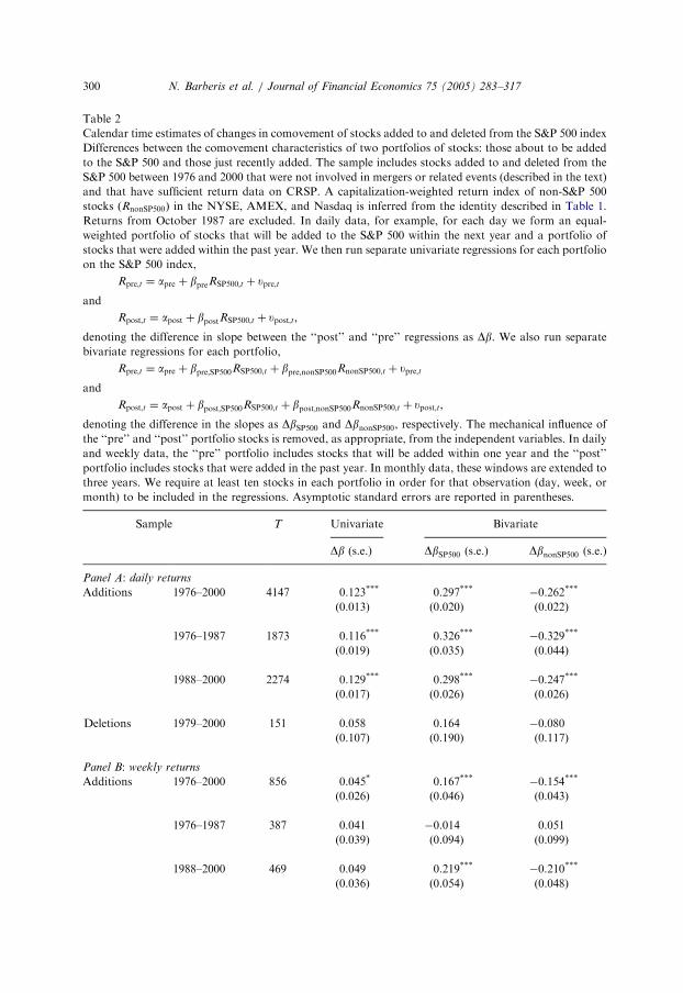
and checking whether bpost;SP5004bpre;SP500 and bpost;nonSP500obpre;nonSP500.Table 2 reports the changes in slope coefficients. The results are again supportive

of the friction- or sentiment-based views. In the univariate regressions, significantincreases in beta occur at the daily and weekly frequencies. In the bivariateregressions, the results for inclusion events are strongly significant at all three datafrequencies, although the results for deletion events are weaker than in the event timetests, turning up no statistically significant effects.

3.5. Alternative explanations: characteristic and industry effects

We now consider some alternative explanations for the results in Table 1. Onepossibility is that stocks in the S&P 500 index differ from other stocks in terms ofsome characteristic, and that the stocks Standard & Poor’s chooses to include arethose increasingly demonstrating that characteristic. If the characteristic is alsoassociated with a cash-flow factor, this may explain our results.The most obvious such characteristic is size. Stocks in the S&P have considerably

higher market capitalizations than stocks outside the index, and the stocks Standard &Poor’s includes in the index have often been growing in size prior to inclusion. Moreover,size is known to be associated with a cash-flow factor: there is a common component tonews about the earnings of large-cap stocks (Fama and French, 1995). Our finding thatS&P betas increase around inclusion may then arise because included stocks are growingin size around inclusion and are therefore increasingly loading on the large-stock cash-flow factor. More generally, this is a story in which inclusion in the S&P coincides with achange in the cash-flow covariance matrix, even if it does not cause it.A related concern is based on industry effects. Suppose that some industry

becomes increasingly dominant in the economy. This increases the fraction of thevalue of the S&P made up by stocks in this industry. Moreover, to keep their indexrepresentative, Standard & Poor’s may start drawing an increasing number of newinclusions from this industry. Since S&P beta is computed using the value-weighted

ARTICLE IN PRESS

Table 2

Calendar time estimates of changes in comovement of stocks added to and deleted from the S&P 500 index

Differences between the comovement characteristics of two portfolios of stocks: those about to be added

to the S&P 500 and those just recently added. The sample includes stocks added to and deleted from the

S&P 500 between 1976 and 2000 that were not involved in mergers or related events (described in the text)

and that have sufficient return data on CRSP. A capitalization-weighted return index of non-S&P 500

stocks ðRnonSP500Þ in the NYSE, AMEX, and Nasdaq is inferred from the identity described in Table 1.

Returns from October 1987 are excluded. In daily data, for example, for each day we form an equal-

weighted portfolio of stocks that will be added to the S&P 500 within the next year and a portfolio of

stocks that were added within the past year. We then run separate univariate regressions for each portfolio

on the S&P 500 index,

Rpre;t ¼ apre þ bpreRSP500;t þ upre;t

and

Rpost;t ¼ apost þ bpostRSP500;t þ upost;t;

denoting the difference in slope between the ‘‘post’’ and ‘‘pre’’ regressions as Db. We also run separate

bivariate regressions for each portfolio,

Rpre;t ¼ apre þ bpre;SP500RSP500;t þ bpre;nonSP500RnonSP500;t þ upre;t

and

Rpost;t ¼ apost þ bpost;SP500RSP500;t þ bpost;nonSP500RnonSP500;t þ upost;t;

denoting the difference in the slopes as DbSP500 and DbnonSP500, respectively. The mechanical influence ofthe ‘‘pre’’ and ‘‘post’’ portfolio stocks is removed, as appropriate, from the independent variables. In daily

and weekly data, the ‘‘pre’’ portfolio includes stocks that will be added within one year and the ‘‘post’’

portfolio includes stocks that were added in the past year. In monthly data, these windows are extended to

three years. We require at least ten stocks in each portfolio in order for that observation (day, week, or

month) to be included in the regressions. Asymptotic standard errors are reported in parentheses.

Sample T Univariate Bivariate

Db (s.e.) DbSP500 (s.e.) DbnonSP500 (s.e.)


Additions 1976–2000 4147 0.123*** 0.297*** �0.262***

(0.013) (0.020) (0.022)

1976–1987 1873 0.116*** 0.326*** �0.329***

(0.019) (0.035) (0.044)

1988–2000 2274 0.129*** 0.298*** �0.247***

(0.017) (0.026) (0.026)

Deletions 1979–2000 151 0.058 0.164 �0.080

(0.107) (0.190) (0.117)


Additions 1976–2000 856 0.045* 0.167*** �0.154***

(0.026) (0.046) (0.043)

1976–1987 387 0.041 �0.014 0.051

(0.039) (0.094) (0.099)

1988–2000 469 0.049 0.219*** �0.210***

(0.036) (0.054) (0.048)


ARTICLE IN PRESS


Sample T Univariate Bivariate

Db (s.e.) DbSP500 (s.e.) DbnonSP500 (s.e.)

Deletions 1979–2000 29 �0.082 �0.162 0.039

(0.193) (0.537) (0.288)


Additions 1976–1998 282 0.018 0.319*** �0.320***

(0.042) (0.073) (0.061)

1976–1987 127 0.019 0.148 �0.143

(0.047) (0.114) (0.099)

1988–1998 155 0.016 0.388*** �0.406***

(0.065) (0.092) (0.075)

Deletions 1979–1998 116 �0.123 �0.255* 0.132

(0.105) (0.166) (0.132)

, , and denote statistical significance at the 1%, 5%, and 10% levels in one-sided tests, respectively.


S&P return, this simultaneity can also lead to effects like those we observe: if Yahoois included in the S&P at precisely the time that other technology stocks in the indexare growing in value—as indeed it was, having been added in December 1999—itmay covary more with the S&P after inclusion than before.We address both these competing explanations with a matching exercise. For each

event stock included in the S&P during our sample period, we search for a‘‘matching’’ stock, drawn from the same industry as the event stock and in the samesize decile both at the time of inclusion and 12 months before inclusion, but which isnot included in the index. Since the matching stock matches the event stock onindustry and on recent growth in market capitalization, it is arguably as good acandidate for inclusion as the event stock itself, but simply happens not to beincluded. If the matching stocks do not demonstrate the same increase (decrease) inS&P (non-S&P) beta as the event stocks, it strengthens the case that the results inTable 1 are due to friction- or sentiment-based comovement, rather than tocharacteristic or industry effects. In the case of deleted stocks, the matching stock is astock in the S&P that matches the deleted stock on industry and recent change inmarket capitalization, but which is not removed from the index.12

12At the monthly frequency, in order to match the window over which the betas are computed, we look

for matching stocks that match the event stock on size both at inclusion and 36 months before inclusion.

At all frequencies, we initially try to match by SIC4 industry code. If no match can be found, we allow the

matching stock to be in the same SIC3 industry class, then to be within one size decile at inclusion, then to

ARTICLE IN PRESS


Fig. 1 and Table 3 contain the results of the matching exercise. Panels A, B, and Cof the figure present results for daily, weekly, and monthly data, respectively. Withineach panel, the top two graphs present results for the event firms, while the bottomtwo correspond to the matching firms. Also, within each panel, the graphs on the leftpresent results for the first half of our sample, while those on the right correspond tothe second half.The graphs use rolling regressions to show how S&P and non-S&P betas change in

event time. Consider the top left graph in Panel A. The solid line shows the meandaily S&P beta and the dashed line shows the mean daily non-S&P beta, re-estimatedeach month using the prior 12 months of daily data. Coefficients plotted to the left ofthe left vertical line therefore use only pre-event returns, while coefficients plotted tothe right of the right vertical line use only post-event returns. Coefficients in betweenuse both pre- and post-event data. To be clear, the steady change in estimated betasbetween the two vertical lines should not be interpreted as a steady change in truebetas. Rather, it arises from mixing data from the pre- and post-event regimes.13

Fig. 1 indicates that whichever frequency we look at, the matching stocks exhibitmuch smaller shifts in betas than do the event stocks. Table 3, which reports thechanges in betas and R2s in univariate and bivariate regressions for event stocksrelative to the analogous changes for matching stocks, confirms this impression. Atthe daily and weekly frequencies, the changes in betas and R2s in univariateregressions and in S&P and non-S&P betas in bivariate regressions remain stronglysignificant across inclusion events, even net of the changes for matching stocks. Atthe monthly frequency, the results are weaker than those in Table 1, but are stillhighly significant in the second subsample.14

In Section 3.3, we noted another prediction of the three friction- or sentiment-based views, namely that the beta shifts around inclusion should decline insignificance at lower frequencies. Table 3 shows that, once we control more carefullyfor fundamentals-based comovement in the bivariate regressions, the residual effect,which is more likely to reflect friction- or sentiment-based comovement, does indeeddecline at lower frequencies. The increase in S&P beta, for example, falls from 0.318at the daily frequency to 0.173 at the monthly one. In Section 3.7, we will be able to

(footnote continued)

be within one size decile 12 months before inclusion, then to be in the same SIC2 industry class, then to be

within two size deciles at inclusion, then to be within two size deciles 12 months before inclusion, and

finally to be within three size deciles 12 months before inclusion. Events for which no such matches can be

found are not included in the matching exercise samples.13In terms of these graphs, the beta changes reported in Table 1 are the average beta as of event month

+12, which uses data from months [+1, +12] minus the average beta as of event month �1, which uses

data from months ½�12;�1�. There are fewer data points in the graph ðN ¼ 169Þ than in Table 1 (N ¼ 196

for additions in the first subsample), however, because the graph includes only event firms with available

return data for a full 24 months after inclusion and for which we are able to find matching firms.14In Table 1, we conduct simulations to correct the standard errors for possible correlation in the

disturbance terms across regressions. This problem affects matching-stock regressions just as much as it

does event-stock regressions, but it does not affect differences in slopes across the two sets of regressions.

The Table 3 standard errors are therefore the usual ones—no simulation-based correction is required.

ARTICLE IN PRESS

1976-1987 additions with matches (N = 169)

0-12 -9 -6 -3 0 3 6 9 12 15 18 21 24 -12 -9 -6 -3 0 3 6 9 12 15 18 21 24

-12 -9 -6 -3 0 3 6 9 12 15 18 21 24

0.2

0.4

0.6

0.8

1

1.2

Event month

Mea

n c

oef

fici

ent


0

0.2

0.4

0.6

0.8

1

1.2

Event month

Mea

n c

oef

fici

ent

1988-2000 matching firms

0

0.2

0.4

0.6

0.8

1

1.2

Event month

Mea

n c

oef

fici

ent

-12 -9 -6 -3 0 3 6 9 12 15 18 21 24


0

0.2

0.4

0.6

0.8

1

1.2

Event month

Mea

n c

oef

fici

ent

(A) Daily returns (solid = S&P 500 coefficient, dash = non S&P coefficient)

Fig. 1. A. Daily returns (solid ¼ S&P 500 coefficient, dash ¼ non S&P coefficient) B. Weekly returns

(solid ¼ S&P 500 coefficient, dash ¼ non S&P coefficient) C. Monthly returns (solid ¼ S&P 500

coefficient, dash ¼ non S&P coefficient). Changes in comovement of stocks added to the S&P 500 Index

and of stocks with matching characteristics. Plots of the mean slope coefficients in bivariate regressions of

returns of stocks added to the S&P 500, and of stocks with matching characteristics, on returns of the S&P

500 Index and the non-S&P 500 rest of the market. The event sample includes stocks added to the S&P 500

that were not involved in mergers or related events (described in the text), which have complete returns

data over the entire event horizon examined in each figure (�12 to +24 months in daily and weekly

returns data and �36 to +72 months in monthly returns data), that remain in the Index for the full post-

event horizon, and for which suitable matching firms exist that have complete data over the same horizon.

Each stock in the event sample is matched with another stock on industry and growth in market

capitalization over the pre-event estimation period. For each added stock j (and each corresponding

matching stock), the bivariate model


is estimated in rolling regressions where sample intervals are ½�12;�1� months for daily and weekly

returns and ½�36;�1� months for monthly returns. Returns on the S&P 500 ðRSP500Þ are from the CRSP

Index on the S&P 500 Universe file. Returns on a capitalization-weighted index of the non-S&P 500 stocks

ðRnonSP500Þ in the NYSE, AMEX, and Nasdaq are inferred from the identity described in Table 1. Returns

from October 1987 are excluded. The mechanical influence of the added stock is removed, as appropriate,

from both independent variables. The means of the event stock coefficients are plotted in event time in the

top half of each panel, and the means of the matching stock coefficients are plotted in the bottom half. The

left vertical line indicates the addition date; coefficients to the left of this line are estimated using only pre-

event data. Coefficients to the right of the right vertical line are estimated using only post-event data. In

between, coefficients are estimated using both pre- and post-event data. Panels A, B, and C show results

for daily, weekly, and monthly returns, respectively.


ARTICLE IN PRESS


0

0.2

0.4

0.6

0.8

1

1.2

Event month

Mea

n c

oef

fici

ent

-12 -9 -6 -3 0 3 6 9 12 15 18 21 24

-12 -9 -6 -3 0 3 6 9 12 15 18 21 24

-12 -9 -6 -3 0 3 6 9 12 15 18 21 24


0

0.2

0.4

0.6

0.8

1

1.2

Event month

Mea

n c

oef

fici

ent


0

0.2

0.4

0.6

0.8

1

1.2

Event month

Mea

n c

oef

fici

ent

-12 -9 -6 -3 0 3 6 9 12 15 18 21 24


0

0.2

0.4

0.6

0.8

1

1.2

Event month

Mea

n c

oef

fici

ent

(B) Weekly returns (solid = S&P 500 coefficient, dash = non S&P coefficient)

Fig. 1. (Continued)


say more about which of the three alternative views is most responsible for thisdeclining effect.At the same time, our matching exercise disrupts the declining pattern of betas

seen in the univariate regressions in Table 1. Table 3 shows that the average increasein beta in the univariate regressions declines from 0.120 to 0.077 as we go from thedaily to the weekly frequency, but then increases to 0.104 at the monthly frequency.Overall, though, accounting for fundamentals-based comovement appears toimprove the fit of our results with the declining significance of beta shifts predictedby the friction- or sentiment-based views.

3.6. Alternative explanations: non-trading effects

Standard & Poor’s explicitly selects stocks that are highly liquid and frequentlytraded for inclusion in the S&P 500 index. Nevertheless, microstructure researchsuggests that our daily frequency results might still have some spurious upward biasdue to non-trading effects (Scholes and Williams, 1977; Dimson, 1979).To see this, suppose that near the end of the trading day, some positive market-

wide information is announced. Since stocks in the S&P are heavily traded, it isprobable that they will trade again before the end of the day: the S&P return for that

ARTICLE IN PRESS


0

0.2

0.4

0.6

0.8

1

1.2

-36 -30 -24 -18 -12 -6 0 6 12 18 24 30 36 42 48 54 60 66 72 -36 -30 -24 -18 -12 -6 0 6 12 18 24 30 36 42 48 54 60 66 72

-36 -30 -24 -18 -12 -6 0 6 12 18 24 30 36 42 48 54 60 66 72

Event month

Mea

n c

oef

fici

ent


0

0.2

0.4

0.6

0.8

1

1.2

Event month

Mea

n c

oef

ficie

nt


-0.2

0

0.2

0.4

0.6

0.8

1

1.2

Event month

Mea

n c

oef

ficie

nt

-36 -30 -24 -18 -12 -6 0 6 12 18 24 30 36 42 48 54 60 66 72


-0.2

0

0.2

0.4

0.6

0.8

1

1.2

Event month

Mea

n c

oef

fici

ent

(C) Monthly returns (solid = S&P 500 coefficient, dash = non S&P coefficient)

Fig. 1. (Continued)


day, RSP500;t, is therefore likely to reflect the good news. A stock outside the index,however, typically trades less often, and may not trade again before the end of theday. As a result, its return for that day, Rj;t, may not reflect the good news. Aregression of Rj;t on RSP500;t then produces an artificially low slope coefficient. Oncethe stock is included in the S&P 500, though, non-trading ceases to be a problem andthe slope coefficient in the regression goes up, just as it does in our results.15

Under the non-trading hypothesis, then, the beta increases we observe occursimply because the typical added stock trades more frequently after inclusion. To seeif our results are indeed due to non-trading, we adopt a test suggested by Vijh (1994).We split the sample of included stocks into two groups: those whose turnoverdecreases after addition and those whose turnover increases. More precisely, for eachstock, we compute the average monthly turnover (share volume divided by sharesoutstanding) over the same pre- and post-event windows used to compute betas, andassign the stock to the first group if its post-event average turnover is lower than itspre-event average turnover, and to the second group otherwise.

15Even though stocks added to the S&P may not trade as often prior to their inclusion as do stocks

already in the index, they invariably still trade at least once a day. Non-trading cannot therefore plausibly

explain the weekly and monthly results in Table 1.

ARTICLE IN PRESS

Table 3

Changes in comovement of stocks added to and deleted from the S&P 500 index relative to matching firms


Index on returns of the S&P 500 index and the non-S&P 500 rest of the market, relative to changes in the

same parameters for matching stocks. Each stock in the event sample is matched with another stock on

industry and growth in market capitalization over the pre-event estimation period. The event sample

includes stocks added to and deleted from the S&P 500 between 1976 and 2000 that were not involved in

mergers or related events (described in the text), that have sufficient return data on CRSP, and for which a

matching stock could be found. For each event stock j, the univariate model




are separately estimated for the pre-event and post-event period, and analogous regressions are run for

each matching stock. Returns on the S&P 500 ðRSP500Þ are from the CRSP Index on the S&P 500 Universe

file. Returns on a capitalization-weighted index of the non-S&P 500 stocks ðRnonSP500Þ in the NYSE,

AMEX, and Nasdaq are inferred from the identity described in Table 1. Returns from October 1987 are

excluded. The mechanical influence of the added or deleted stock is removed from the independent

variables as appropriate. For the univariate regression model, we examine the mean change in slope and fit

across the event date for event stocks minus the corresponding quantities for matching stocks, DDb and

DDR2. For the bivariate model, we examine the mean change in slopes for event stocks minus the

corresponding quantities for matching stocks, DDbSP500 and DDbnonSP500. The pre-event and post-event

estimation periods are ½�12;�1� and [+1,+12] months for daily and weekly returns and ½�36;�1� and[+1,+36] months for monthly returns. Panels A, B, and C show results for daily, weekly, and monthly

returns, respectively. Asymptotic standard errors are reported in parentheses.


DDb (s.e.) DDR2 (s.e.) DDbSP500 (s.e.) DDbnonSP500 (s.e.)


Additions 1976–2000 435 0.120*** 0.040*** 0.318*** �0.289***

(0.022) (0.006) (0.035) (0.042)

1976–1987 189 0.109*** 0.033*** 0.262*** �0.257***

(0.028) (0.008) (0.051) (0.065)

1988–2000 246 0.129*** 0.046*** 0.361*** �0.313***

(0.032) (0.007) (0.047) (0.055)

Deletions 1979–2000 36 �0.098 �0.012 �0.298** 0.271

(0.081) (0.013) (0.142) (0.193)


Additions 1976–2000 434 0.077** 0.028*** 0.208*** �0.146**

(0.037) (0.009) (0.070) (0.070)

1976–1987 188 0.086* 0.026* 0.202* �0.162

(0.047) (0.015) (0.113) (0.114)

1988–2000 246 0.070 0.030*** 0.212** �0.134

(0.055) (0.012) (0.087) (0.088)


ARTICLE IN PRESS



DDb (s.e.) DDR2 (s.e.) DDbSP500 (s.e.) DDbnonSP500 (s.e.)

Deletions 1979–2000 36 �0.013 �0.030 �0.616** 0.771**

(0.157) (0.020) (0.251) (0.285)


Additions 1976–1998 300 0.104** 0.011 0.173* �0.090

(0.047) (0.013) (0.103) (0.091)

1976–1987 162 0.054 0.008 0.054 �0.011

(0.060) (0.020) (0.145) (0.125)

1988–1998 138 0.163** 0.015 0.313** �0.183

(0.073) (0.020) (0.144) (0.133)

Deletions 1979–1998 18 0.236 0.057 0.438 �0.133

(0.156) (0.041) (0.315) (0.266)

, , and denote statistical significance at the 1%, 5%, and 10% levels in one-sided tests, respectively.


If non-trading is driving our results, we should only see increases in S&P beta afterinclusion for the second group of stocks—those whose turnover increases—while forthe first group, we should see decreases.16 The three friction- or sentiment-basedviews of comovement, on the other hand, predict increases in S&P beta for both

groups. Table 4 presents the results. It shows that in both the univariate andbivariate regressions, there are strongly statistically significant increases in S&P betaseven for stocks whose turnover decreases after inclusion. Non-trading cannottherefore be the primary driver of our daily frequency results.The results in Table 4 do, however, suggest some role for non-trading. In the

univariate regressions, the shifts in S&P beta are considerably larger in Panel B,which is what we would expect if non-trading played some part in our results. In thebivariate regressions, the ratios of the absolute increase in S&P beta to the absolutedecrease in non-S&P beta are larger in Panel B, which is again what would beexpected in the presence of non-trading. We can think of the quantitative effect offriction- or sentiment-based comovement on S&P betas, controlling for non-trading,as some average of the results in Panels A and B—somewhere between 0.083 and0.194 in the univariate case, and somewhere between 0.313 and 0.350 in the bivariatecase. Clearly, these effects will be strongly statistically significant and economicallysubstantial.

16Strictly speaking, we should see increases in S&P beta for those included stocks whose turnover moves

closer to the value-weighted turnover of stocks already in the S&P. Since, as Vijh (1994) shows, almost all

included stocks have turnover lower than this value-weighted average, both before and after inclusion, the

prediction is more simply made in terms of an increase in turnover.

ARTICLE IN PRESS

Table 4

Changes in comovement of stocks added to and deleted from the S&P 500 index by change in trading

volume


Index on returns of the S&P 500 index and the non-S&P 500 rest of the market. The sample includes stocks

added to and deleted from the S&P 500 between 1976 and 2000 that were not involved in mergers or

related events (described in the text) and that have sufficient return and trading volume data on CRSP. For

each event stock j, the univariate model




are separately estimated for the pre- and post-event period. Returns from October 1987 are excluded. The

mechanical influence of the added or deleted stock is removed from the independent variables as

appropriate. For the univariate regression model, we examine the mean change in slope across the event

date Db, and the mean change in fit DR2. For the bivariate model, we examine the mean changes in the

slopes, DbSP500 and DbnonSP500. The pre- and post-event estimation samples are ½�12;�1� and [+1,+12]

months of daily data. Average pre- and post-event monthly turnover (volume divided by shares

outstanding) are computed over these same intervals and are used to identify the direction in trading

volume. Panel A reports results for stocks whose turnover decreased. Panel B reports results for stocks

whose turnover increased. Standard errors are adjusted using simulations to account for cross-correlation,

and are reported in parentheses.


Db DR2 DbSP500 DbnonSP500(s.e.) (s.e.) (s.e.) (s.e.)

Panel A: turnover decrease

Additions 1976–2000 151 0.083** 0.062*** 0.313*** �0.374***

(0.037) (0.009) (0.048) (0.055)

1976–1987 65 0.054* 0.052*** 0.248*** �0.294***

(0.036) (0.013) (0.073) (0.086)

1988–2000 86 0.105** 0.070*** 0.362*** �0.434***

(0.060) (0.012) (0.063) (0.071)

Panel B: turnover increase

Additions 1976–2000 295 0.194*** 0.045*** 0.350*** �0.307***

(0.025) (0.007) (0.033) (0.042)

1976–1987 122 0.089*** 0.035*** 0.344*** �0.342***

(0.031) (0.010) (0.050) (0.062)

1988–2000 173 0.269*** 0.052*** 0.354*** �0.282***

(0.036) (0.009) (0.044) (0.056)


respectively.


In summary, non-trading takes a small bite out of the daily frequency results inTable 1. Characteristic and industry effects, on the other hand, reduce the strength ofthe monthly frequency results in Table 1, but have little impact on the daily andweekly findings. Taken together, Tables 3 and 4 show that, even after adjusting forboth non-trading and matching-firm effects, there is still strong residual evidence for

ARTICLE IN PRESS


friction- or sentiment-based comovement. The daily and weekly results remainstrongly significant, as do the monthly results in the second subsample.

3.7. Distinguishing the category, habitat, and information diffusion views

So far, we have argued that a substantial part of the shift in betas around inclusionis due to friction- or sentiment-based comovement of some kind, but we have notidentified which of the three mechanisms—category, habitat, or informationdiffusion—might be playing a more significant role. In this section, we attempt toshed some light on this.Using return data alone, it is difficult to distinguish between the category and

habitat views, but it may still be possible to isolate the effect of informationdiffusion. The reason is that the information diffusion view makes a prediction notshared by the category and habitat views, namely that there should be positive cross-autocorrelation between S&P and non-S&P returns: good news about aggregateearnings is incorporated into the prices of S&P stocks today, but only with somedelay into the prices of non-S&P stocks.This suggests that we can identify the effect of information diffusion by including

leading and lagged S&P and non-S&P returns in the univariate and bivariateregressions (14) and (15), a technique proposed by Dimson (1979). Specifically, fordaily frequency data, we estimate the regressions

Rj;t ¼ aj þX5s¼�5

bðsÞj RSP500;tþs þ vj;t ð20Þ

and


bðsÞj;SP500RSP500;tþs þX5s¼�5

bðsÞj;nonSP500RnonSP500;tþs þ vj;t ð21Þ

both before and after each inclusion and deletion event, thereby including five leadsand lags. The changes in the quantities17

X5s¼�5

wðsÞbðsÞj ;X5s¼�5

wðsÞbðsÞj;SP500 andX5s¼�5

bwðsÞbðsÞj;nonSP500 ð22Þ

across event dates can be interpreted as the beta shifts that would occur in a worldwithout any delay in the incorporation of information: in other words, they capturethe component of the results in Table 1 due only to category and habitat effects andnot to information diffusion. If they are closer to zero than the daily beta shifts inTable 1, it suggests that information diffusion is in part driving our results. If theyare still nonzero, however, it suggests that information diffusion cannot explain theentire shift in betas, but that category and habitat effects are also at work.

17The wðsÞ, wðsÞ and bwðsÞ variables in these formulas are weights that correct the Dimson (1979)

expressions for autocorrelation in S&P and non-S&P returns. The required weights are derived by Fowler

and Rorke (1983). In our data, they are all close to 1.

ARTICLE IN PRESS


Panel A of Table 5 reports the average changes in the quantities in (22) acrossevent dates. Comparing these numbers to those in Table 1, we see that informationdiffusion accounts for about a third of the economic magnitude of our univariateresults and that even after removing its effects, the residual, attributable to categoryand habitat effects, remains strongly significant. It also shows that informationdiffusion accounts for a much larger fraction, perhaps two-thirds, of the economicmagnitude of the bivariate regression results. Even though the increase in S&P betaremains quantitatively large, particularly in the later subsample, the standard errorsare so large that statistical significance drops considerably.18

Panel B shows, for the full sample of inclusions, how the components of the threequantities in (22) change after inclusion. For example, the row labeled t reports the

changes in wð0Þbð0Þj , wð0Þbð0Þj;SP500, and bwð0Þbð0Þj;nonSP500; the row labeled t � 1 reports the

changes in wð�1Þbð�1Þj , wð�1Þbð�1Þj;SP500, and bwð�1Þbð�1Þj;nonSP500; and so on for the other rows.

These numbers are consistent with information diffusion playing some role in ourresults. The loading of the added stock’s return on the previous day’s S&P returndeclines after inclusion—wð�1Þbð�1Þj and wð�1Þbð�1Þj;SP500 fall by 0.080 and 0.118,respectively—consistent with the idea that before inclusion, the stock incorporatesmarket-wide information a day after the S&P, but as soon as it is included, it does sothe same day. The rise, after inclusion, in the sensitivity of the added stock’s return tothe following day’s non-S&P return can be interpreted the same way.Panel B shows that the pattern predicted by the information diffusion view—a

drop in the sensitivity, wð�sÞbð�sÞj and wð�sÞbð�sÞ

j;SP500, of the added stock’s return tolagged S&P returns—is barely detectable beyond just a one-day lag in the univariateregressions and beyond a two-day lag in the bivariate regressions. In other words,although information does appear to enter non-S&P returns more slowly than S&Preturns, the delay is short. The rapid attenuation of the information diffusion effectin Panel B means that it can play only a minimal role at lower frequencies.In our discussion of Table 3, we noted that the shifts in beta across inclusion are

weaker at lower frequencies. This pattern disappears after taking out the effect ofinformation diffusion: the 0.113 and 0.110 univariate and bivariate shifts in daily

S&P betas, reported in Table 5, are not statistically different from our best estimatesof the univariate and bivariate shifts in monthly S&P beta, reported in Table 3 as0.104 and 0.173. The frequency effect in Table 3 is therefore probably driven mostlyby information diffusion: if information can take two or three days to be fullyincorporated, there will be a more pronounced change in beta at the daily frequencythan at weekly or monthly frequencies. The residual shift in beta, after controllingfor information diffusion, is relatively stable across frequencies. Since this residual ismost likely attributable to the category and habitat views, it suggests that the noise-trader sentiment assumed by those mechanisms does not mean-revert quickly, butrather is quite persistent.

18The component of our results that we attribute to slow information diffusion could also be due to a

closely related mechanism in which it is market-wide sentiment, and not just market-wide cash-flow news,

that is incorporated more quickly into some stocks than into others.

ARTICLE IN PRESS

Table 5

Changes in comovement of stocks added to and deleted from the S&P 500 index: Information diffusion

effects (five leads and lags)

Changes in the slope and the fit of regressions of daily returns of stocks added to and deleted from the S&P

500 index on daily returns of the S&P 500 index and the non-S&P 500 rest of the market, using five leads

and lags in daily returns to adjust beta for information diffusion effects as suggested by Dimson (1979) and

Fowler and Rorke (1983). The sample includes stocks added to and deleted from the S&P 500 between

1976 and 2000 that were not involved in mergers or related events (described in the text) and that have

sufficient return data on CRSP. For each event stock j, the univariate model


b sð Þj RSP500;tþs þ uj;t



ðb sð Þj;SP500RSP500;tþs þ b sð Þ

j;nonSP500RnonSP500;tþsÞ þ uj;t

are separately estimated for the pre-event and post-event period. Returns on the S&P 500 ðRSP500Þ are from

the CRSP Index on the S&P 500 Universe file. Returns on a capitalization-weighted index of the non-S&P

500 stocks ðRnonSP500Þ in the NYSE, AMEX, and Nasdaq are inferred from the identity described in Table

1. Returns from October 1987 are excluded. The mechanical influence of the added or deleted stock is

removed from the independent variables as appropriate. In Panel A, we report the mean difference

between the pre-event and post-event Dimson beta (defined as the sum of the lag, contemporaneous, and

lead beta coefficients, weighted to account for index autocorrelation as in Fowler and Rorke, 1983). In

Panel B, we report the mean difference between the pre-event and post-event components of the Dimson

beta (again weighted to account for index autocorrelation). Standard errors are adjusted using simulations

to account for cross-correlation, and are reported in parentheses.

Sample N (Panel A) Univariate Bivariate

term (Panel B) Db (s.e) DR2 (s.e) DbSP500 (s.e) DbnonSP500 (s.e.)

Panel A: Dimson beta (5 leads and lags)

Additions 1976–2000 449 0.113*** 0.038*** 0.110 �0.013

(0.046) (0.005) (0.093) (0.078)

1976–1987 190 0.021 0.026*** 0.045 0.001

(0.055) (0.008) (0.116) (0.135)

1988–2000 259 0.180*** 0.046*** 0.158* �0.022

(0.068) (0.007) (0.110) (0.092)

Deletions 1979–2000 76 �0.016 �0.012* �0.627** 0.533**

(0.168) (0.008) (0.354) (0.255)

Panel B: components of Dimson beta (5 leads and lags)

Additions 1976–2000 t � 5 �0.002 �0.025 0.051***

(0.012) (0.021) (0.022)

t � 4 0.038*** 0.059*** �0.039*

(0.013) (0.025) (0.029)

t � 3 0.009 �0.002 0.018

(0.012) (0.025) (0.027)

t � 2 �0.005 �0.043** 0.023

(0.012) (0.023) (0.027)

t � 1 �0.080*** �0.118*** 0.149***

(0.014) (0.025) (0.031)

t 0.150*** 0.310*** �0.310***

(0.021) (0.028) (0.037)


ARTICLE IN PRESS


Sample N (Panel A) Univariate Bivariate

term (Panel B) Db (s.e) DR2 (s.e) DbSP500 (s.e) DbnonSP500 (s.e.)

t þ 1 �0.006 �0.070*** 0.068**

(0.013) (0.025) (0.031)

t þ 2 0.007 �0.055** 0.056**

(0.010) (0.024) (0.028)

t þ 3 �0.021** �0.036* 0.048**

(0.012) (0.023) (0.026)

t þ 4 0.023** 0.048** �0.025

(0.012) (0.024) (0.026)

t þ 5 0.000 0.043** �0.053**

(0.012) (0.023) (0.023)


respectively.


4. Conclusion

We present two broad theories of return comovement and examine them empiricallyusing data on additions to the S&P 500. The traditional theory, fundamentals-basedcomovement, is derived from frictionless economies with rational investors andattributes comovement in returns to correlation in news about fundamental value. Thealternative theory argues that, due to market frictions or noise-trader sentiment, returncomovement is delinked from fundamentals. We consider three specific variants ofsuch ‘‘friction-based’’ or ‘‘sentiment-based’’ comovement, and label them thecategory, habitat, and information diffusion views.In earlier work on S&P inclusions during 1975–1989, Vijh (1994) finds that stocks

added to the index experience a significant increase in beta after inclusion. In thispaper, we first show that by applying a univariate analysis similar to Vijh’s to thenew data now available, we uncover considerably stronger effects. We then showthat in bivariate regressions that also include the return of non-S&P stocks, the rise inS&P beta is altogether larger than anything in the univariate regressions, that thislast effect is also stronger in more recent data, and that exactly the opposite patternholds for stocks deleted from the index. We also find that in both univariate andbivariate regressions, the effects are somewhat weaker at lower frequencies.Our findings cannot easily be explained by the fundamentals-based view of

comovement, but fit with the friction- or sentiment-based views. We make someprogress in determining the relative importance of the three specific mechanisms wepropose. Slow diffusion of information, for example, appears to account for arelatively small part of the beta shifts in the univariate regressions, but for up to two-thirds of the beta shifts in the daily bivariate regressions. Overall, our evidence addsto the growing range of phenomena identified by financial economists that reveal theimportance of market frictions and noise-trader sentiment for valuation.

ARTICLE IN PRESS


Appendix A

A.1. Derivation of predictions 1 and 2

For simplicity, we assume that the cash-flow covariance matrix SD takes a specificform, although the predictions also hold for more general structures. In particular,we suppose that the cash-flow shock to an asset has three components: a market-wide cash-flow shock, a group-specific cash-flow shock that affects assets in onegroup but not the other, and a completely idiosyncratic cash-flow shock specific tothe asset. Formally, for i 2 X ,

ei;t ¼ cMf M;t þ cSf X ;t þ

ffiffiffiffiffiffiffiffiffiffiffiffiffiffiffiffiffiffiffiffiffiffiffiffiffiffiffiffiffiffið1� c2

M � c2SÞ

qf i;t; ð23Þ

and for j 2 Y ,

ej;t ¼ cMf M;t þ cSf Y ;t þ

ffiffiffiffiffiffiffiffiffiffiffiffiffiffiffiffiffiffiffiffiffiffiffiffiffiffiffiffiffiffið1� c2

M � c2SÞ

qf j;t; ð24Þ

where f M;t is the market-wide shock, f X ;t and f Y ;t are the group-specific shocks, andf i;t and f j;t are idiosyncratic shocks; cM and cS are constants that control the relativeimportance of the three components. Each shock has unit variance and is orthogonalto the other shocks.Consider first the reduced-form model for the category and habitat views, Eqs.

(4)–(5). Suppose that asset n þ 1 is reclassified from Y into X, and that at the samemoment, asset 1 is reclassified from X into Y. Before reclassification,

DPX ;t ¼ eX ;t þ DuX ;t ð25Þ

DPY ;t ¼ eY ;t þ DuY ;t ð26Þ

DPnþ1;t ¼ enþ1;t þ DuY ;t; ð27Þ

where

ek;t ¼1

n

Xl2k

el;t; k ¼ X ;Y ; ð28Þ

while after reclassification, DPX ;t and DPY ;t are still given by (25) and (26), but now

DPnþ1;t ¼ enþ1;t þ DuX ;t: ð29Þ

Using the standard formula for regression coefficients, we find that as n ! 1, theprobability limit of the OLS estimate of bnþ1 in the regression

DPnþ1;t ¼ anþ1 þ bnþ1DPX ;t þ vnþ1;t ð30Þ

is given by

bnþ1 ¼c2M þ 2s2uru

c2M þ c2

S þ 2s2uð31Þ

ARTICLE IN PRESS


before reclassification, and by

bnþ1 ¼c2M þ 2s2u

c2M þ c2

S þ 2s2uð32Þ

afterwards, thereby confirming that bnþ1 increases after reclassification as claimed inPrediction 1. Moreover, since varðDPnþ1;tÞ and varðDPX ;tÞ are unchanged afterreclassification, the increase in bnþ1 also implies an increase in the R2 of regression(30) after inclusion.Similarly, we find that as n ! 1, the probability limits of the OLS estimates of

bnþ1;X and bnþ1;Y in the regression

DPnþ1;tþ1 ¼ anþ1 þ bnþ1;XDPX ;tþ1 þ bnþ1;YDPY ;tþ1 þ vnþ1;tþ1 ð33Þ

are given by

bnþ1;X ¼ 0; bnþ1;Y ¼ 1 ð34Þ

before reclassification and by

bnþ1;X ¼2s2uð1� ruÞ

c2S þ 2s2uð1� ruÞ

; bnþ1;Y ¼c2S

c2S þ 2s2uð1� ruÞ

ð35Þ

afterwards, thereby confirming Prediction 2.Now consider the reduced-form model for the information diffusion view, Eqs.

(7)–(8). Suppose that asset n þ 1 is reclassified from Y into X, and that at the samemoment, asset 1 is reclassified from X into Y. Before reclassification,

DPX ;t ¼ eX ;t ð36Þ

DPY ;t ¼ meY ;t þ ð1� mÞeY ;t�1 ð37Þ

DPnþ1;t ¼ menþ1;t þ ð1� mÞenþ1;t�1; ð38Þ

where ek;t is defined in (28), while after reclassification, DPX ;t and DPY ;t are still givenby (36) and (37), but now

DPnþ1;t ¼ enþ1;t: ð39Þ

This implies that as n ! 1, the probability limit of the OLS estimate of bnþ1 inregression (30) is given by

bnþ1 ¼mc2

M

c2M þ c2

S

ð40Þ

before reclassification, and by

bnþ1 ¼c2M

c2M þ c2

S

ð41Þ

afterwards, thereby confirming that bnþ1 increases after reclassification as claimed inPrediction 1. Moreover, since varðDPnþ1;tÞ and varðDPX ;tÞ are unchanged after

ARTICLE IN PRESS


reclassification, the increase in bnþ1 also implies an increase in the R2 of regression(30) after inclusion.Similarly, we find that as n ! 1, the probability limits of the OLS estimates of

bnþ1;X and bnþ1;Y in regression (33) are given by

bnþ1;X ¼ 0; bnþ1;Y ¼ 1 ð42Þ

before reclassification and by

bnþ1;X ¼ð1� mÞ2c2

Mðc2M þ c2

SÞ

m2c2Sð2c

2M þ c2

SÞ þ ð1� mÞ2ðc2M þ c2

SÞ2; ð43Þ

bnþ1;Y ¼mc2

Sð2c2M þ c2

SÞ

m2c2Sð2c

2M þ c2

SÞ þ ð1� mÞ2ðc2M þ c2

SÞ2

ð44Þ

afterwards. It is straightforward to check that if momn, where

mn ¼ðc2

M þ c2SÞ

2

c2Sð2c

2M þ c2

SÞ þ ðc2M þ c2

SÞ2; ð45Þ

then bnþ1;X increases after inclusion, while bnþ1;Y falls. If, moreover, m ¼ mnn, where

mnn ¼c2M þ c2

S

3c2M þ 2c2

S

; ð46Þ

then the increase in bnþ1;X is precisely equal in magnitude to the decrease in bnþ1;Y .Prediction 2 does not therefore follow as generally from Eqs. (7)–(8) as it does fromEqs. (4)–(5), but it is nonetheless derivable from both reduced-form models.

A.2. Standard error computations

As discussed in Section 3.2, correlation in the residuals vj;t across different stocksmeans that the fDbjgj¼1;...;N are not independent, thereby requiring an adjustment tothe standard error of the test statistic Db that would be obtained assumingindependence. To gauge, at least approximately, how large this correction should be,we generate a large number of artificial data sets and use them to compare thedistribution of the test statistic in the case where there is correlation in residuals tothe distribution in the case where there is none.We simulate the artificial data as follows. We generate the S&P and non-S&P

returns from

RSP500;t ¼ RM;t þ wSP500;t ð47Þ

RnonSP500;t ¼ RM;t þ wnonSP500;t; ð48Þ

ARTICLE IN PRESS


where

RM;t � Nð0;s2MÞ ð49Þ

wSP500;t � Nð0;s2SÞ ð50Þ

wnonSP500;t � Nð0;s2SÞ; ð51Þ

with all three variables assumed i.i.d. over time and independent of all othervariables. We generate the included stock’s return from

Rj;t ¼ RnonSP500;t þ RF ;t þ wj;t; ð52Þ

where

RF ;t � Nð0;s2F Þ ð53Þ

wj;t � Nð0;s2 � s2M � s2S � s2F Þ; ð54Þ

with both variables assumed i.i.d. over time and independent of all other variables.RF ;t is a common factor in the returns of included stocks that leads to correlation inthe disturbances vj;t across regressions. The variance of wj;t in (54) ensures that theoverall variance of the included stock’s return in (52) is given by s2.For each data frequency, we set sM to match the standard deviation of the market

return; sS to generate a correlation between RSP500;t and RnonSP500;t that matches theempirical value; and s to match the typical standard deviation of an individual stock.The one parameter that remains is sF , and we set it at whatever value generates afirst-order autocorrelation in the fDbjgj¼1;...;N equal to that in the actual data.With parameter values assigned, we now generate many artificial data sets. Each

data set consists of an S&P return and a non-S&P return spanning the entire lengthof the sample and, taking the case of daily data, return data for 455 included stocksfor the two years around their respective event dates. The spacing of event dates inthe artificial data matches the spacing in the actual data. With a large number ofartificial data sets in hand, we can construct the distribution of the test statistic Dbfor the case where the fDbjgj¼1;...;N are not independent. We then compare this to thedistribution of the test statistic for the case of sF ¼ 0, in which the fDbjgj¼1;...;N areuncorrelated. Finally, we inflate the standard errors in the tables by the impliedcorrection factor.

References

Barberis, N., Shleifer, A., 2003. Style investing. Journal of Financial Economics 68, 161–199.

Barberis, N., Shleifer, A., Wurgler, J., 2002. Comovement. NBER working paper no. 8895.

Bodurtha, J., Kim, D., Lee, C.M., 1995. Closed-end country funds and U.S. market sentiment. Review of

Financial Studies 8, 879–918.

Cooper, M., Dimitrov, O., Rau, P.R., 2001. A rose.com by any other name. Journal of Finance 56,

2371–2388.

De Long, J.B., Shleifer, A., Summers, L., Waldmann, R., 1990. Noise trader risk in financial markets.

Journal of Political Economy 98, 703–738.

ARTICLE IN PRESS


Denis, D.K., McConnell, J.J., Ovtchinnikov, A.V., Yu, Y., 2003. S&P 500 index additions and earnings

expectations. Journal of Finance 58, 1821–1840.

Dimson, E., 1979. Risk measurement when shares are subject to infrequent trading. Journal of Financial

Economics 7, 197–227.

Fama, E., French, K., 1995. Size and book-to-market factors in earnings and returns. Journal of Finance

50, 131–155.

Fowler, D., Rorke, C.H., 1983. Risk measurement when shares are subject to infrequent trading. Journal

of Financial Economics 12, 279–283.

French, K., Roll, R., 1986. Stock return variances: the arrival of information and the reaction of traders.

Journal of Financial Economics 17, 5–26.

Froot, K., Dabora, E., 1999. How are stock prices affected by the location of trade? Journal of Financial


Goetzmann, W., Massa, M., 2003. Index funds and stock market growth. Journal of Business 76, 1–28.

Goldberger, A., 1991. A Course in Econometrics. Harvard University Press, Cambridge, MA.

Gompers, P., Metrick, A., 2001. Institutional investors and equity prices. Quarterly Journal of Economics

116, 229–259.

Greenwood, R., 2004. Short- and long-term demand curves for stocks: theory and evidence on the

dynamics of arbitrage. Journal of Financial Economics, Article in Press.

Greenwood, R., Sosner, N., 2002. Trading patterns and excess comovement of stock returns. Unpublished

working paper, Harvard University.

Hardouvelis, G., LaPorta, R., Wizman, T., 1994. What moves the discount on country equity funds? In:

Frankel, J. (Ed.), The Internationalization of Equity Markets. The University of Chicago Press,

Chicago.

Harris, L., Gurel, E., 1986. Price and volume effects associated with changes in the S&P 500: new evidence

for the existence of price pressure. Journal of Finance 41, 851–860.

Kaul, A., Mehrotra, V., Morck, R., 2000. Demand curves for stocks do slope down: new evidence from an

index weights adjustment. Journal of Finance 55, 893–912.

Lamont, O., Thaler, R., 2003. Can the market add and subtract? Mispricing in tech stock carveouts.

Journal of Political Economy 111, 227–268.

Lee, C., Shleifer, A., Thaler, R., 1991. Investor sentiment and the closed-end fund puzzle. Journal of

Finance 46, 75–110.

Lynch, A., Mendenhall, R., 1997. New evidence on stock price effects associated with changes in the S&P

500 index. Journal of Business 70, 351–383.

Mitchell, M., Pulvino, T., Stafford, E., 2002. Limited arbitrage in equity markets. Journal of Finance 57,

551–584.

Mullainathan, S., 2002. Thinking through categories. Unpublished working paper, Massachusetts

Institute of Technology.

Pindyck, R., Rotemberg, J., 1990. The excess comovement of commodity prices. Economic Journal 100,

1173–1189.

Scholes, M., Williams, J., 1977. Estimating betas from nonsynchronous data. Journal of Financial


Shleifer, A., 1986. Do demand curves for stocks slope down? Journal of Finance 41, 579–590.

Shleifer, A., Vishny, R., 1997. The limits of arbitrage. Journal of Finance 52, 35–55.

Vijh, A., 1994. S&P 500 trading strategies and stock betas. Review of Financial Studies 7, 215–251.

Wurgler, J., Zhuravskaya, K., 2002. Does arbitrage flatten demand curves for stocks? Journal of Business

75, 583–608.

Comovement - Faculty Directoryfaculty.som.yale.edu/nicholasbarberis/sap_jnl.pdf ·...

Documents

Transcript of Comovement - Faculty Directoryfaculty.som.yale.edu/nicholasbarberis/sap_jnl.pdf ·...