Session 1: Introduction to Complex Survey Design

Anthony RaffertyUniversity of Manchester

anthony.rafferty@manchester.ac.uk

Overview of Day

• Session 1: Basic Concepts• Session 2: Implications of Complex design

for Estimation (design effects) and model and design-based approaches (MCS)

• Workshop 1: Clustering• Workshop 2: Stratification• Workshop 3: Further Topics

Random sampling• A simple random sample without

replacement (SRS) Every potential subset of n units has an equal probability of being selected as the sample.

• To ensure representative sample and guard against selection bias.

• Systematic sample to proxy SRS. Random start point and fixed interval across sampling frame

• Sampling Frame: Postal Address File (PAF); Land and Property Services Agency’s (LPSA) (Northern Ireland)

Use of Samples• Samples are used to estimate population

parameters (e.g. mean height, income).

• Simple random sampling allows us to use standard methods for point and variance estimates – (standard Stata commands assume SRS)

• However, ESDS Government surveys frequently include ‘complex’ sample designs features (e.g. clustering & stratification).

Precision & Bias of Estimates• Sampling error refers to the variation in

estimates calculated from different samples – Variance; Standard Errors; Confidence Intervals– Smaller confidence interval=more precise estimate– Stratification and clustering influence ‘correct’

calculation: – Design-based; model-based approaches

• Bias: Difference between estimator's value based on sample and the true value of the population parameter being estimated. An estimate is said to be biased if the centre of its distribution does not coincide with the population value.

Precise

Imprecise

Important Factors affecting precision/ sampling error

• Sample size

• Sample design (stratification and clustering)

Design Effect

• Measure of effects of clustering and stratification on standard errors/ confidence intervals

• The design effect (Deff) is the relative size of the design based variance to the Simple random sample variance:– = Var (.)design/ Var (.) srs

• The square root of the design effect gives the design factor (deft). This puts things back into the scale of the standard errors

Interpretation

• We will consider how to incorporate complex design and calculate design effects

• Interpretation of Deft• Deft = 1:No Effect of sample design on

standard error• Deft>1: Sample design inflates the

standard error of the estimate• Deft<1: Sample design increases

efficiency (reduces s.e.) of estimate.

Clustering

• Rather than taking a random sample of the overall population, breaking down of a population first into a higher level characteristic or unit than the population elements, such as by geographical unit.

• A random sample of these units is randomly selected then population elements are drawn from the selected units. (Lohr, p 24.)

Why Cluster?

• Geographically concentrating interviews is cost-effective

• On the downside: ‘positive’ effect on Deft: Increases standard error relative to equivalent simple random sample

One-stage cluster sample

• Random sample of a population unit is selected, such as postal code sectors, then all population elements (e.g. individuals) in the sample of clusters are taken as the element level sample.

• All elements in selected PSU units included in sample

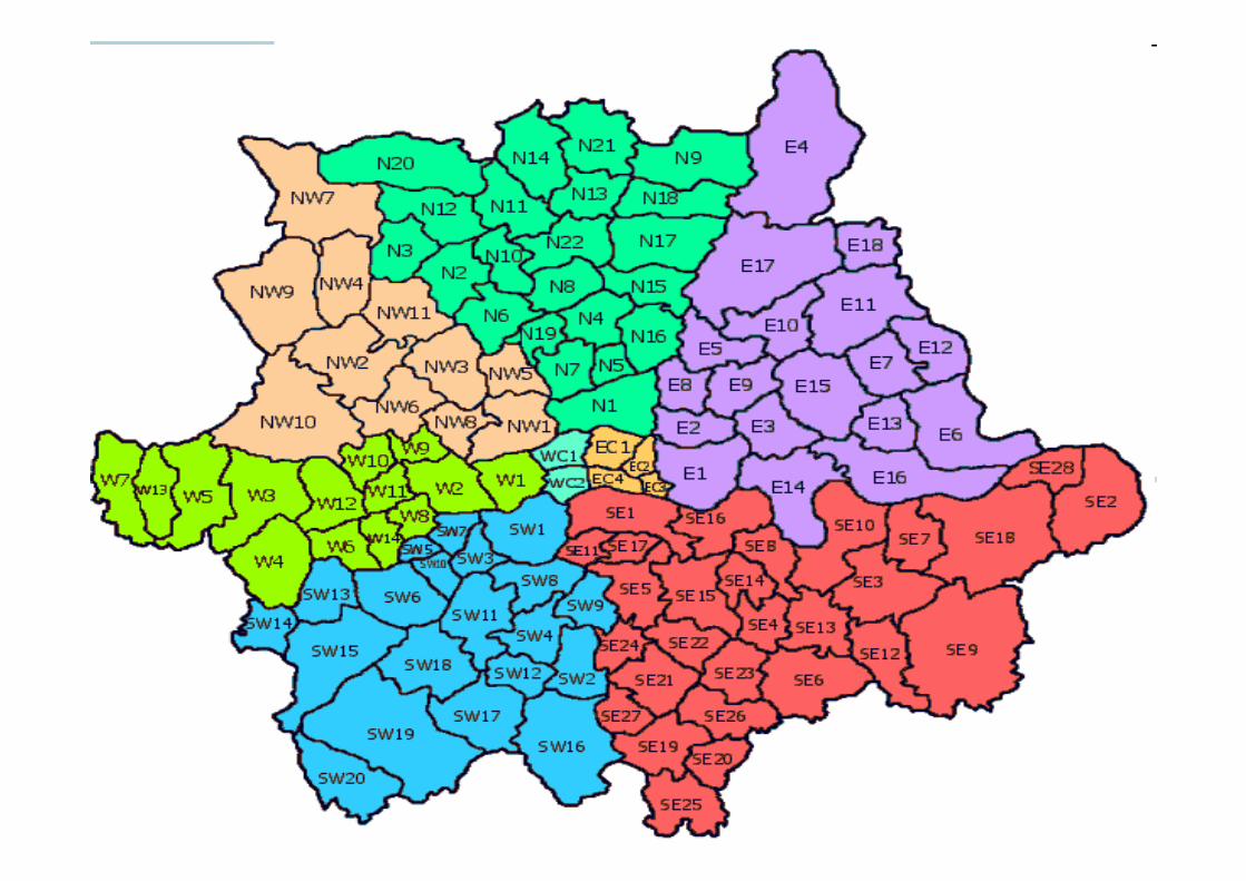
Primary Sampling Units (PSUs)

Know your postcode!M13 9PL

• M13 is post code district• M13 9 is postcode sector (used for

PSUs)• M13 9 PL is delivery point (used to

identify addresses).

• Map example higher geography for PSUs then usually used.

Two-stage Example

• Primary Sampling Unit (PSU) • Secondary Sampling Unit (SSU)• At the first stage, a random sample of

PSUs (e.g. postcode sectors) is selected.• In the second stage, a random sample of

SSUs (e.g.households) is selected within postal code sectors.

• Individuals (‘population elements’) are then selected within households. In this design, adults are clustered in households, and households are clustered in postcode sectors.

Stratification• In stratified sampling, the population is

partitioned into groups (strata) based on variables, such as regions, or car ownership (yes/no), and a sample is selected by some design (e.g. randomly) within each strata.

• Prior knowledge about some characteristics of sampling units in the population is thus used to control the number of units sampled within each stratum

Stratification• Implicit/ explicit

– Explicit: group population by strata then random sample in different stratum

– Implicit: Sort sampling frame by stratification variable(s) and take random starting point then fixed intervals

• Proportionate/disproportionate– Disproportionate: Ethnicity booster samples;

Child booster samples– Weighting adjusts for disproportionate sample

Sample frame of 4

M M F F• Take 50 per cent random sample– Could end up with two men or two

women– We know sample frame is 50/50

male/female

So stratify (explicity)

M M F F• Separate men and women…

M M F F

Then randomly select 1 M 1 F

M M F F

SAMPLE

Sample:

M F

Or implicit stratification

• Order sample frame in a line: women, then men (but order of two men and two women is random):

F F M M

implicit stratification

• Starting point random (as women order random)

F F M M

implicit stratification

• Work out interval to achieve 50 per cent sample across sampling frame

F F M M

implicit stratification

Sample

F M

Why Stratify?• Enforce representativeness

• Small efficiency gain (proportionate stratification). i.e. reduces standard errors/negative effect on Deft.

• Efficiency gain in disproportionate stratification depends on level of variance in disproportionate stratum. +/-

Problem with sample?

Explicit stratum

Explicit stratumPSUs

Common Stratifiers

• Government Office Region; • Local Authority • Car ownership; • % according to UK census in non-manual

occupations• Level of disadvantage

• Can combine different strata variables and implicit and explicit stratification

Post-stratification

• Weighting method that adjusts for any differences between the survey data and the population in terms of a few key population variables (e.g. age and sex). The aim is to reduce any bias due to sampling error and non-response effects.

Example: Health Survey of England 2007

• The sample for the HSE was drawn in two stages. At the first stage a random sample of primary sampling units (PSUs), based on postcode sectors, was selected. Within each selected PSU, a random sample of postal addresses (known as delivery points) was then drawn.

• The list of PSUs in England was ordered by local authority and, within each local authority, by the percentage of households in the 2001 Census with a head of household in a non-manual occupation (NS-SEC groups 1-3).

HSE07• The sample of PSUs was then selected by

sampling from the list at fixed intervals from a random starting point. 900 PSUs were selected with probability proportional to the total number of addresses within them.

• Once selected the 900 PSUs were randomly allocated to one of two groups; 720 PSUs were allocated to the core sample and 180 PSUs were allocated to the additional child boost sample. The core PSUs contained sampled addresses for both the core and child boost sample, the additional child boost PSUs only.

What is the design?

• One-stage/two stage?• Disproportionate/proportionate

stratification?• Implicit/explicit stratification?

Acknowledgements

Thanks to Leen Van de Casteele (CCSR/Social Statistics) for guidance and help on topics, and lecture materials from Dep. of Social Statistics

(Manchester) Masters course module on Advanced Survey Methods.

http://www.socialsciences.manchester.ac.uk/disciplines/socialstatistics/index.html

Appendix: Samples

• Simple random sample with replacement (SRSWR), one unit is randomly selected from the population then put back into the population and a second unit is drawn. The procedure is repeated until the desired n units are obtained, and due to replacement there may be duplicates in the sample (i.e. the same unit may be used twice).

ge cluster_b = cluster

list cluster_b area if cluster_b == 66list cluster_b area if cluster_b == 137

replace cluster_b = 65 in 5438replace cluster_b = 65 in 11007/11030replace cluster_b = 136 in 11765/11768replace cluster_b = 136 in 12637/12644

Workshop 1: Clustering• Declaring the complex sample design

features of you survey to Stata using the svyset command. – Primary sampling units and weights

• Summary statistics and cross-tabulations• Conducting sub-population analysis

correctly.• Basic modelling and estimating design

effects using svyset:– Effects of clustering on standard errors and on

the statistical significance of findings.

Intra-cluster correlation• The homogeneity of the cluster is measured

by the intra-cluster correlation coefficient (ICC, or rho).

• If individuals in a cluster have more in common than with people in general then the rho will be bigger than zero.

• As rho increase so does standard errors. If people are all alike in a cluster, but different from people in other clusters, then there is a greater risk of drawing a sample that is different from the overall population.

• Rho is used to calculate design effects

Interpretation

• We will consider how to incorporate complex design and calculate design effects

• Interpretation of Deft• Deft = 1:No Effect of sample design on

standard error• Deft>1: Sample design inflates the

standard error of the estimate• Deft<1: Sample design increases

efficiency (reduces s.e.) of estimate.

Workshop 2: Stratification

• The effects of stratification on standard errors.

• How to inspect and, if necessary, prepare a stratification variable for inclusion in your analysis using the svydes command.

Workshop 3: Further Topics

• Incorporating (or ignoring) multi-stage design (e.g. secondary sampling unit features) into your analysis and the ‘ultimate cluster method’.

• Comparing linearization and replicate methods.

• Brief comparison of model-based and design-based approaches

• We are using the 06 HSE data.

SSU• Finite population correction (fpc) (1-

n/N)• used because in small samples, the greater

our sample size the more information we have about the population the smaller the variances. For samples taken from extremely large populations, the fpc will approximate to 1, whereas other samples, the size of the sample determine the precision of the estimator (sse Lohr, pg. 33).

Linearization• A linear estimator is a linear function of the

sample observations. In simple random samples many estimators are linear estimators where the sample size n is fixed.

• However, in cluster sampling, situations arise where the sample size cannot be assumed fixed across different clusters, for example, in one-stage clustering where the sizes of clusters Bi vary. (see Lehtonen and Pahkinen, 1994, pg 138.).

• The taylor series linearization method provides a linear approximation of the non-linear estimators, to which linear estimator formulas for estimating variances are applied.

Replicate Methods• In replication approaches, a defined

number (K) of subsets (replicate samples) of the full sample are selected, and the estimation procedure is repeated for each subsample and the variance calculated.

• Information on the sum of these subset samples is used to estimate variances.Statistics of interest are calculated for each subsample (‘replicate statistics’) and then the variability between these subsample replicate statistics are used to estimate the variance of the full sample statistic.

Replicate Methods

• Because the formulation of the probability samples is based upon the complex design, unbiased, design corrected variance estimates can be derived.

Replicate Methods

• Replication techniques include ‘Balanced Repeated Replication (BRR)’ (designed for where there are only two sampling units pre strata) and ‘Jackknife’.

• In the Jackknife technique, the replicate samples are obtained by successively omitting one sampling unit fro each stratum and performing estimates

• Bootstrap is also used (currently not built in to svyset command suite).

Jackknife• In unstratified surveys one PSU at a

time is deleted and the others reweighted

• to keep the same total weight (known as the JK1 jackknife). For stratified designs the jackknife removes one PSU at a time, but reweights only the other PSUs in the same stratum. Jackknife can be used where there are more than two PSUs per stratum.

Preference between methods

• Often similar performance between linearization and replicate techniques.

• Check findings robust by comparing different methodologies?

Wrapping up (1)

• PSU arguably (in most cases) most important aspect of complex sample design to take into account- don’t forget weighting though on disproportionately stratified samples.

• Many Government surveys deposited without PSU.

• No PSU? Contact ESDS Government

Model vs design-based approaches

• model based more efficient (smaller standard errors)

• however assumptions on population structure, wrong model, wrong results

• stratification is included as covariate, however we may be interested in an estimate unadjusted by the stratification variable(s)

• design based arguably is easier for the inexperienced

• although there may be circumstances where your sampling units are of substantive interest

Textbooks & Resources

• ESRC Research Methods Programme Resource:

• http://www2.napier.ac.uk/depts/fhls/peas/index.htm

• Lohr, S. (1999) “Sampling Design and Analysis”, Pacific Grove: Duxbury.

• Lehtonen, R. and Pahkinen, E. (1994) “Practical Methods for the Design and Analysis of Complex Surveys, New York, John Wiley.

The important last slide…

Helpdesk:govsurveys@esds.ac.uk

(0161)275 1980

Website:http://www.esds.ac.uk/government

Jisc list:esds-govsurveys@jiscmail.ac.uk