Flux Balance Analysis

Evangelos Simeonidis

v.simeonidis@manchester.ac.uk

Metabolic Engineering

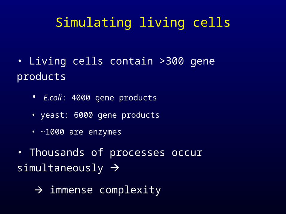
Simulating living cells

• Living cells contain >300 gene products

• E.coli: 4000 gene products

• yeast: 6000 gene products

• ~1000 are enzymes

• Thousands of processes occur simultaneously

immense complexity

How can Metabolic Engineering cope with this complexity?

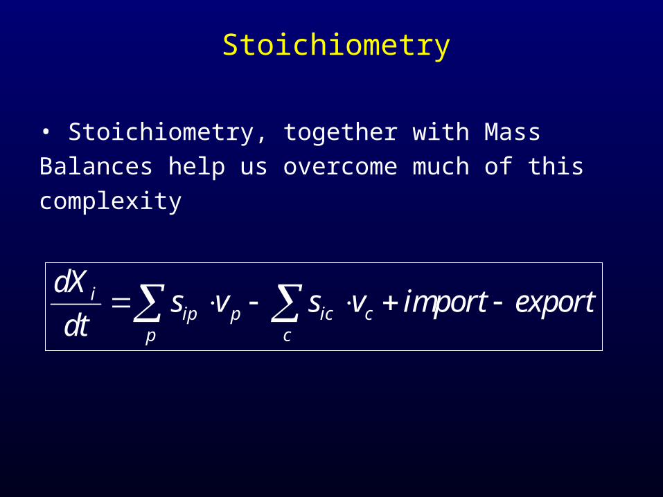
Stoichiometry

• Stoichiometry, together with Mass Balances help us

overcome much of this complexity

iip p ic c

p c

dXs v s v import export

dt

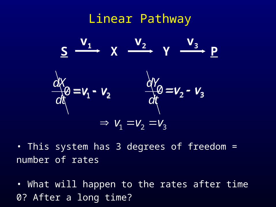
Linear Pathway

• This system has 3 degrees of freedom = number of rates

• What will happen to the rates after time 0? After a long time?

• The system is said to be in “steady state”

1 2

dXv v

dt

S X PYv1 v2 v3

2 3

dYv v

dt

1 20 v v 2 30 v v

1 2 3v v v

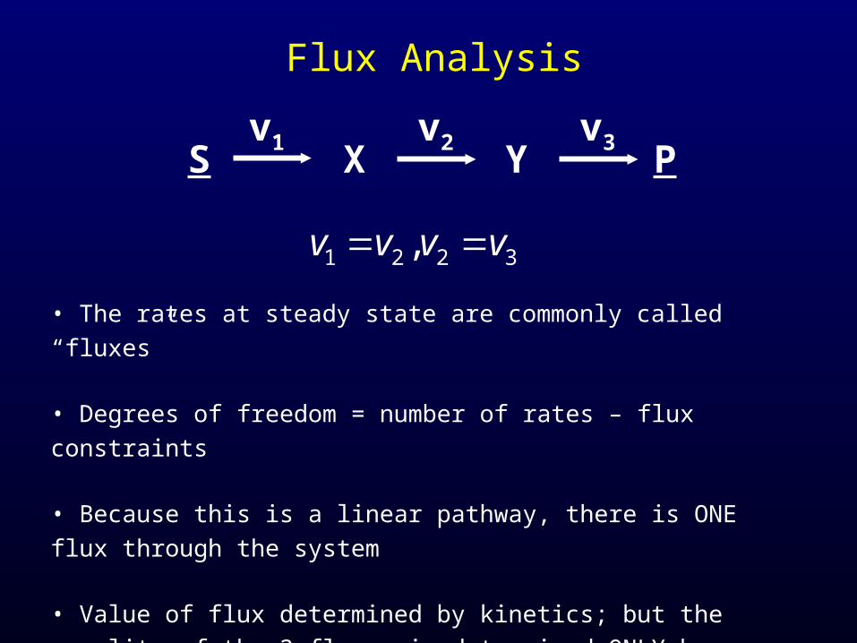
Flux Analysis

• The rates at steady state are commonly called “fluxes”

• Degrees of freedom = number of rates – flux constraints

• Because this is a linear pathway, there is ONE flux through the system

• Value of flux determined by kinetics; but the equality of the 3 fluxes is

determined ONLY by stoichiometry

How do we increase the yield (production) of P?

S X PYv1 v2 v3

1 2 2 3,v v v v

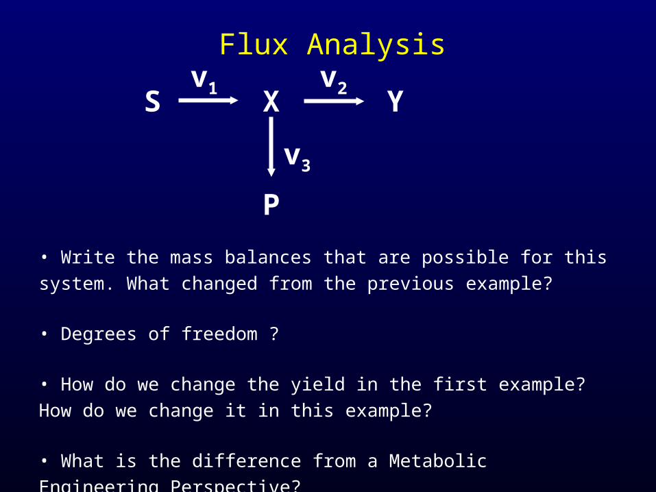
Flux Analysis

• Write the mass balances that are possible for this system. What changed

from the previous example?

• Degrees of freedom ?

• How do we change the yield in the first example? How do we change it in

this example?

• What is the difference from a Metabolic Engineering Perspective?

S X

P

Yv1 v2

v3

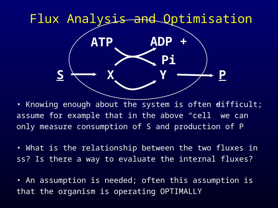
Flux Analysis and Optimisation

• Knowing enough about the system is often difficult; assume for example that

in the above “cell” we can only measure consumption of S and production of P

• What is the relationship between the two fluxes in ss? Is there a way to

evaluate the internal fluxes?

• An assumption is needed; often this assumption is that the organism is

operating OPTIMALLY

• e.g. assume the above organism optimal with respect to energetic efficiency

S X PY

ATP ADP + Pi

Topics covered

• Constraint-based approach to metabolic modelling

• Mathematics behind FBA: Optimisation

• Mathematical examples

Introduction

• A major goal of systems biology is to relate genome

sequence to cell physiology

• This requires the identification of the components and

their interactions in the system + mathematical modelling

• Small molecule metabolism is the best described

molecular network in the cell and there are various

computational tools to model its behaviour

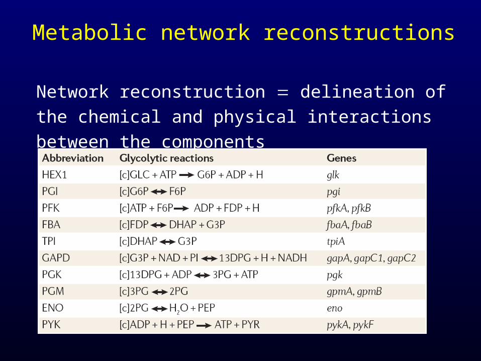
Metabolic network reconstructions

Network reconstruction delineation of the chemical and

physical interactions between the components

Metabolic network reconstructions

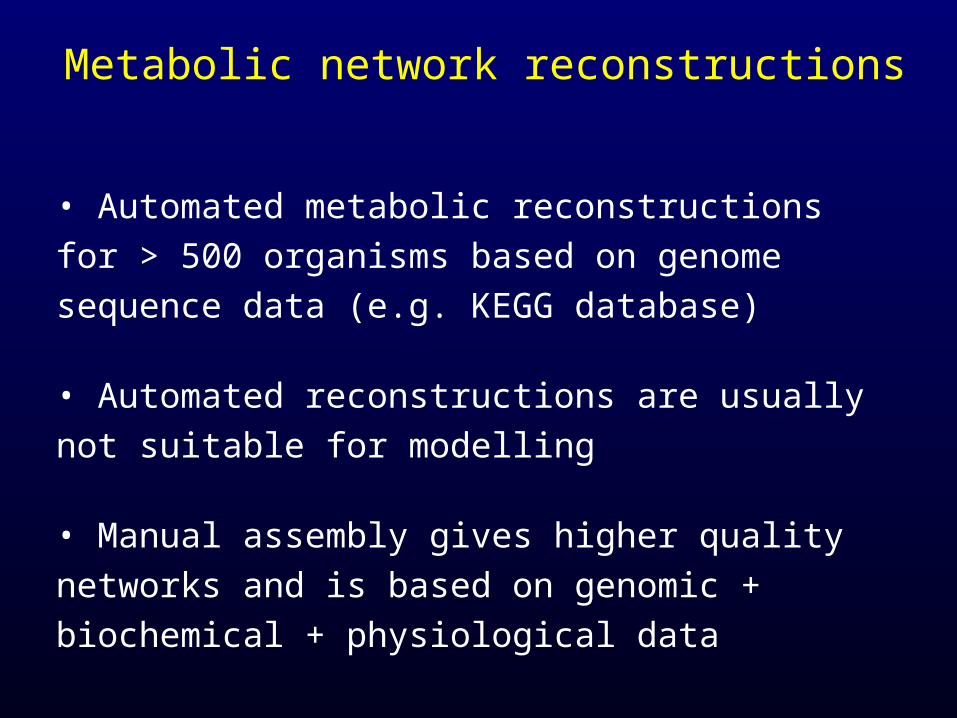
• Automated metabolic reconstructions for > 500 organisms

based on genome sequence data (e.g. KEGG database)

• Automated reconstructions are usually not suitable for

modelling

• Manual assembly gives higher quality networks and is

based on genomic + biochemical + physiological data

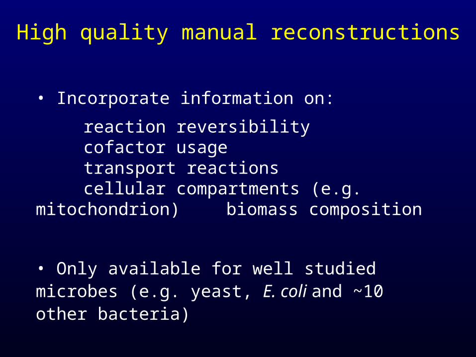
• Incorporate information on:

reaction reversibilitycofactor usagetransport reactionscellular compartments (e.g. mitochondrion)

biomass composition

• Only available for well studied microbes (e.g. yeast, E. coli and ~10 other bacteria)

High quality manual reconstructions

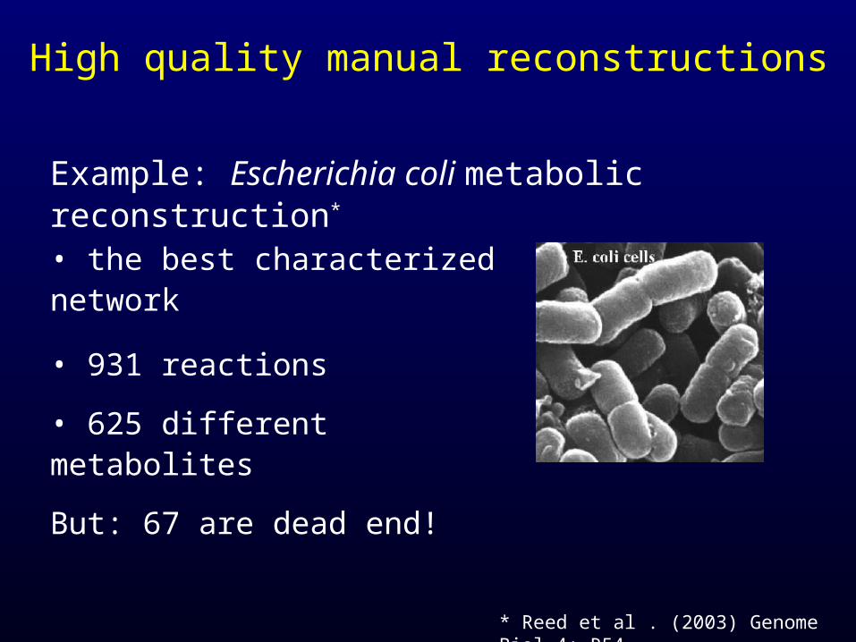
Example: Escherichia coli metabolic reconstruction*

• the best characterized network

• 931 reactions

• 625 different metabolites

But: 67 are dead end!

High quality manual reconstructions

* Reed et al . (2003) Genome Biol 4: R54

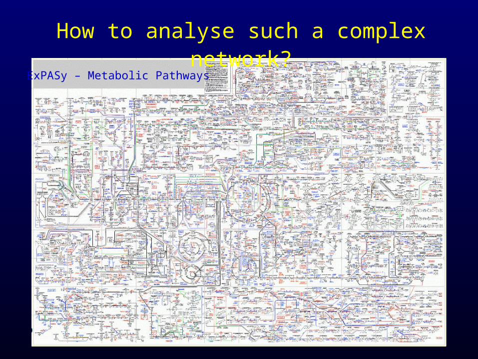
How to analyse such a complex network?

ExPASy – Metabolic Pathways

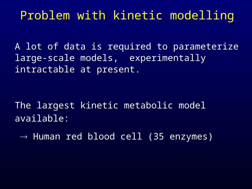
Problem with kinetic modelling

A lot of data is required to parameterize large-scale models, experimentally intractable at present.

The largest kinetic metabolic model available:

Human red blood cell (35 enzymes)

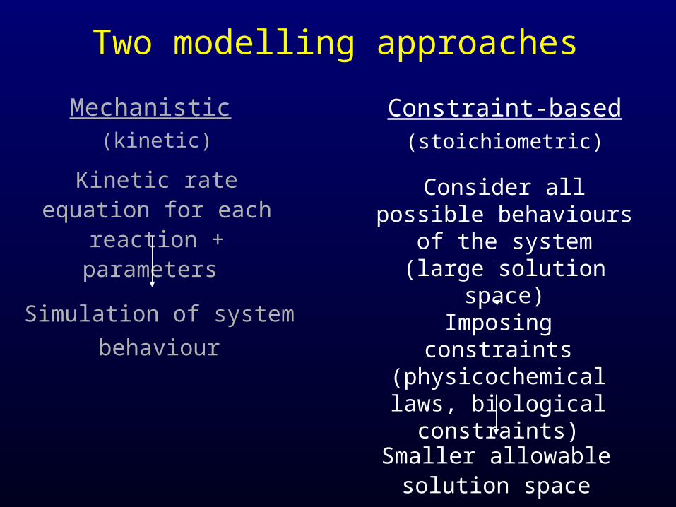
Two modelling approaches

Kinetic rate equation for each reaction + parameters

Simulation of system

behaviour

Mechanistic (kinetic)

Constraint-based (stoichiometric)

Consider all possible behaviours of the system

(large solution space)

Imposing constraints (physicochemical laws, biological constraints)

Smaller allowable solution space

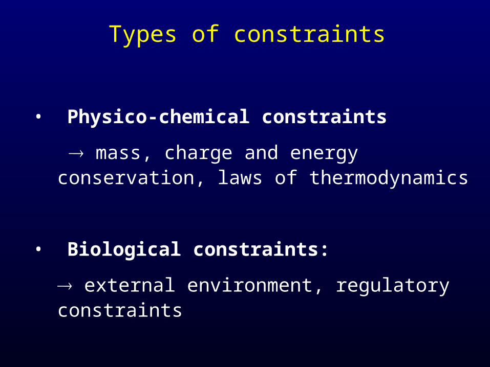
Types of constraints

• Physico-chemical constraints

mass, charge and energy conservation, laws of thermodynamics

• Biological constraints:

external environment, regulatory constraints

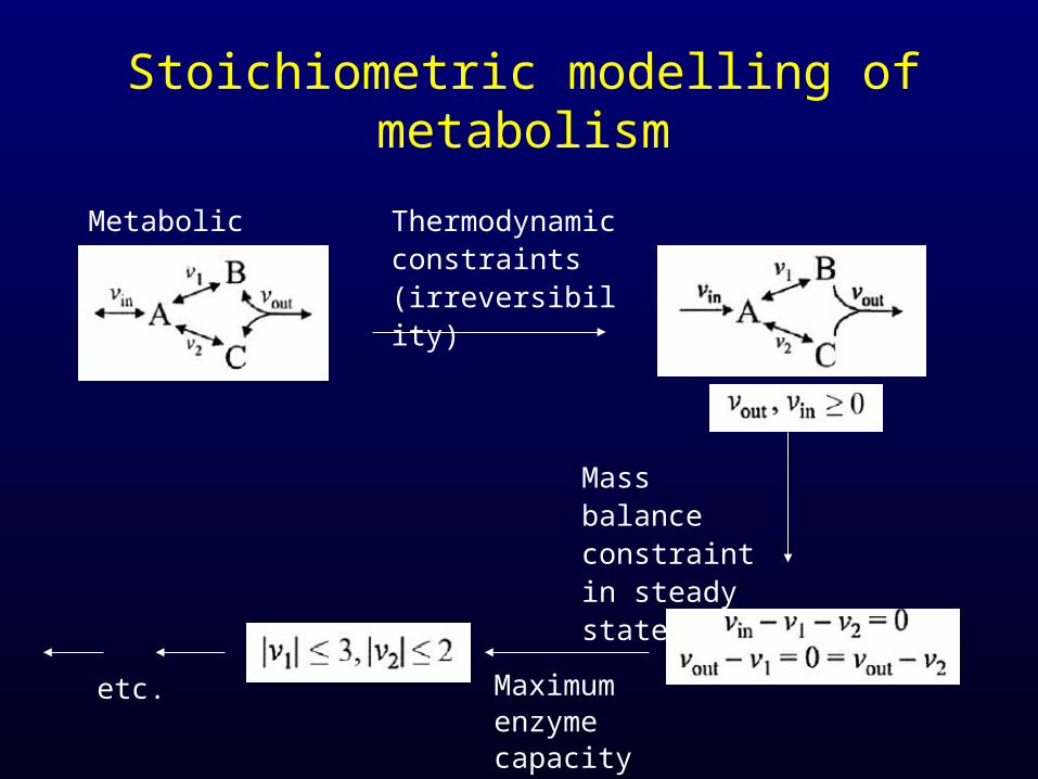
Stoichiometric modelling of metabolism

Metabolic network Thermodynamic constraints (irreversibility)

Mass balance constraint in steady state

Maximum enzyme capacity

etc.

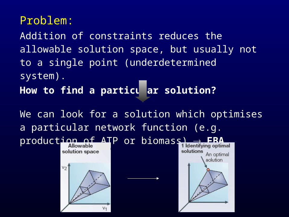
Problem:Addition of constraints reduces the allowable solution space, but usually not to a single point (underdetermined system).

How to find a particular solution?

We can look for a solution which optimises a particular network function (e.g. production of ATP or biomass) FBA

Topics covered

• Constraint-based approach to metabolic modelling

• Mathematics behind FBA: Optimisation

• Mathematical examples

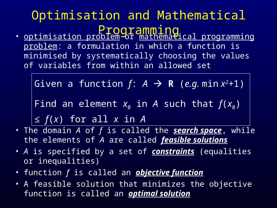
Optimisation and Mathematical Programming

• optimisation problem or mathematical programming problem: a formulation in which a function is minimised by systematically choosing the values of variables from within an allowed set

Given a function f: A R (e.g. min x2+1)

Find an element x0 in A such that f(x0) ≤ f(x) for all x in A

• The domain A of f is called the search space, while the elements of A are called feasible solutions

• A is specified by a set of constraints (equalities or inequalities)

• function f is called an objective function

• A feasible solution that minimizes the objective function is called an optimal solution

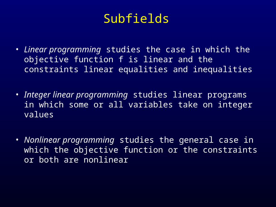
Subfields

• Linear programming studies the case in which the objective function f is linear and the constraints linear equalities and inequalities

• Integer linear programming studies linear programs in which some or all variables take on integer values

• Nonlinear programming studies the general case in which the objective function or the constraints or both are nonlinear

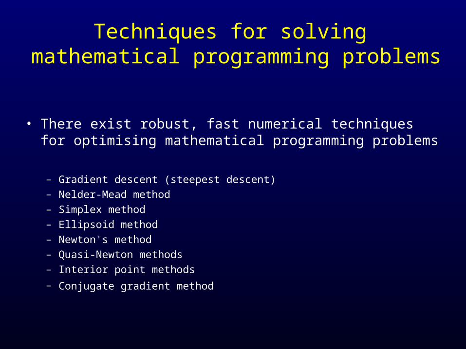
Techniques for solving mathematical programming problems

• There exist robust, fast numerical techniques for optimising mathematical programming problems

– Gradient descent (steepest descent) – Nelder-Mead method – Simplex method – Ellipsoid method – Newton's method – Quasi-Newton methods – Interior point methods

– Conjugate gradient method

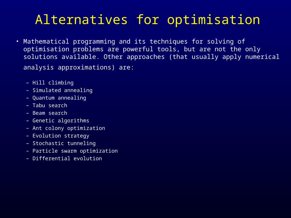
Alternatives for optimisation

• Mathematical programming and its techniques for solving of optimisation problems are powerful tools, but are not the only solutions available. Other approaches (that usually

apply numerical analysis approximations) are:

– Hill climbing – Simulated annealing – Quantum annealing – Tabu search – Beam search – Genetic algorithms – Ant colony optimization – Evolution strategy – Stochastic tunneling – Particle swarm optimization– Differential evolution

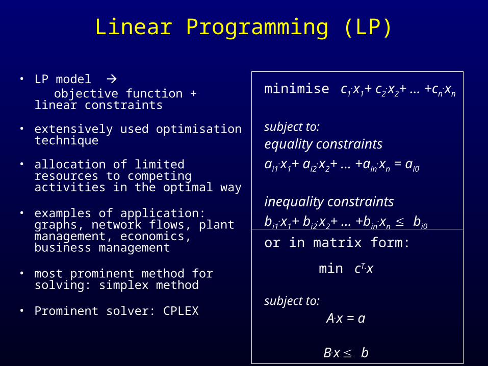
Linear Programming (LP)

• LP model objective function + linear constraints

• extensively used optimisation technique

• allocation of limited resources to competing activities in the optimal way

• examples of application: graphs, network flows, plant management, economics, business management

• most prominent method for solving: simplex method

• Prominent solver: CPLEX

minimise c1.x1+ c2

.x2+ … +cn.xn

subject to:

equality constraints

ai1.x1+ ai2

.x2+ … +ain.xn = ai0

inequality constraints

bi1.x1+ bi2

.x2+ … +bin.xn bi0

or in matrix form:

min cT.x

subject to:

A.x = a

B.x b

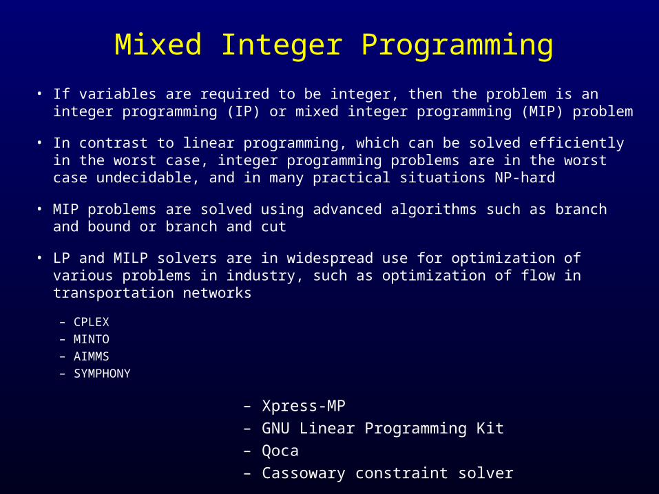
Mixed Integer Programming

• If variables are required to be integer, then the problem is an integer programming (IP) or mixed integer programming (MIP) problem

• In contrast to linear programming, which can be solved efficiently in the worst case, integer programming problems are in the worst case undecidable, and in many practical situations NP-hard

• MIP problems are solved using advanced algorithms such as branch and bound or branch and cut

• LP and MILP solvers are in widespread use for optimization of various problems in industry, such as optimization of flow in transportation networks

– CPLEX – MINTO– AIMMS – SYMPHONY – Xpress-MP

– GNU Linear Programming Kit

– Qoca

– Cassowary constraint solver

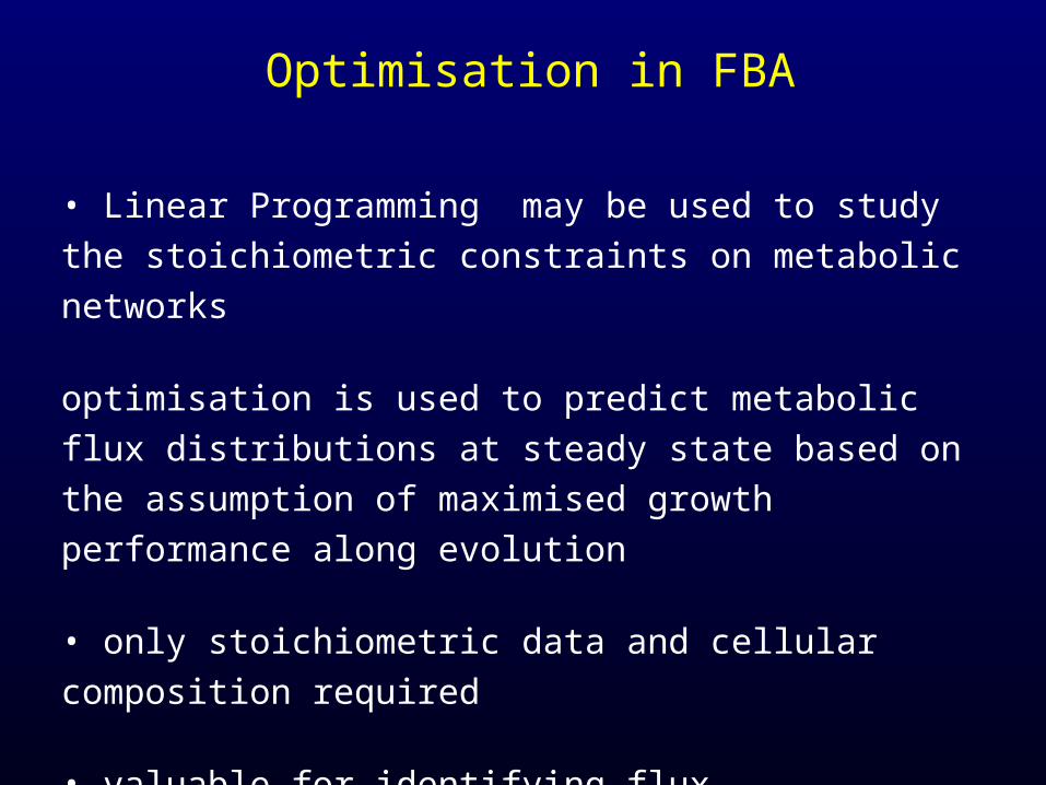
Optimisation in FBA

• Linear Programming may be used to study the stoichiometric

constraints on metabolic networks

optimisation is used to predict metabolic flux distributions at

steady state based on the assumption of maximised growth

performance along evolution

• only stoichiometric data and cellular composition required

• valuable for identifying flux distribution boundaries for the

metabolic function of cellular systems

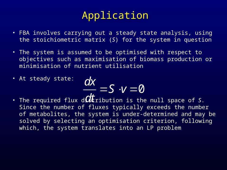
Application

• FBA involves carrying out a steady state analysis, using the stoichiometric matrix (S) for the system in question

• The system is assumed to be optimised with respect to objectives such as maximisation of biomass production or minimisation of nutrient utilisation

• At steady state:

• The required flux distribution is the null space of S. Since the number of fluxes typically exceeds the number of metabolites, the system is under-determined and may be solved by selecting an optimisation criterion, following which, the system translates into an LP problem

0dx

S vdt

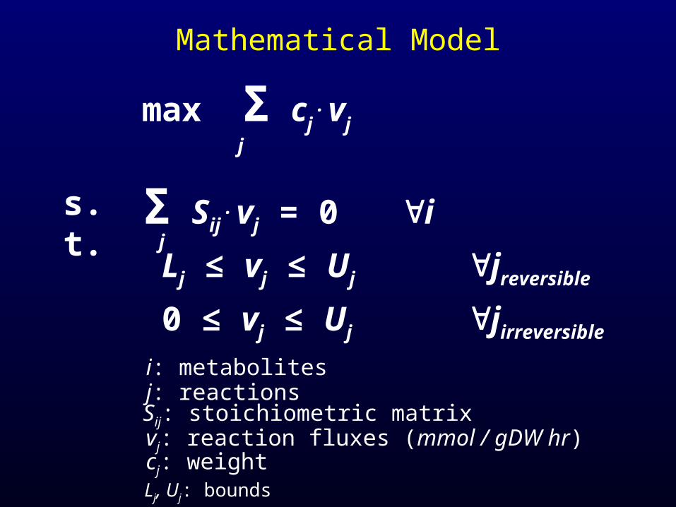
Mathematical Model

max Σ cj . vj

Σ Sij . vj = 0 i

Lj ≤ vj ≤ Uj jreversible

0 ≤ vj ≤ Uj jirreversible

Sij: stoichiometric matrixvj: reaction fluxes (mmol / gDW hr)cj: weight

j

j

i: metabolitesj: reactions

s.t.

Lj, Uj: bounds

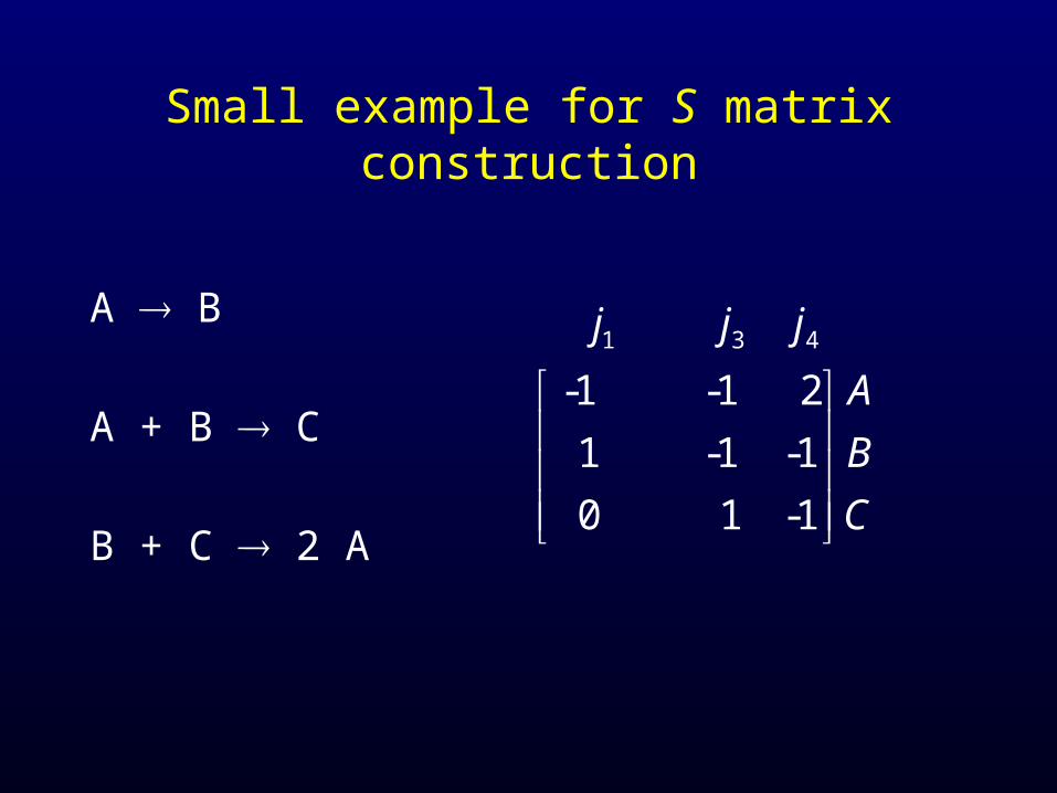
Small example for S matrix construction

A B

A + B C

B + C 2 A

1 3 4

-1 -1 2

1 -1 -1

0 1 -

1

j j j

A

B

C

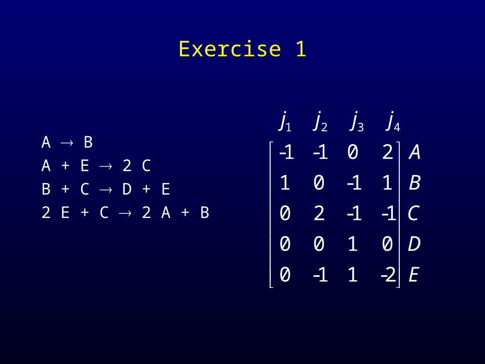
Exercise 1

A B

A + E 2 C

B + C D + E

2 E + C 2 A + B

1 2 3 4

-1 -1 0 2

1 0 -1 1

0 2 -1 -1

0 0 1 0

0 -1 1 -2

j j j j

A

B

C

D

E

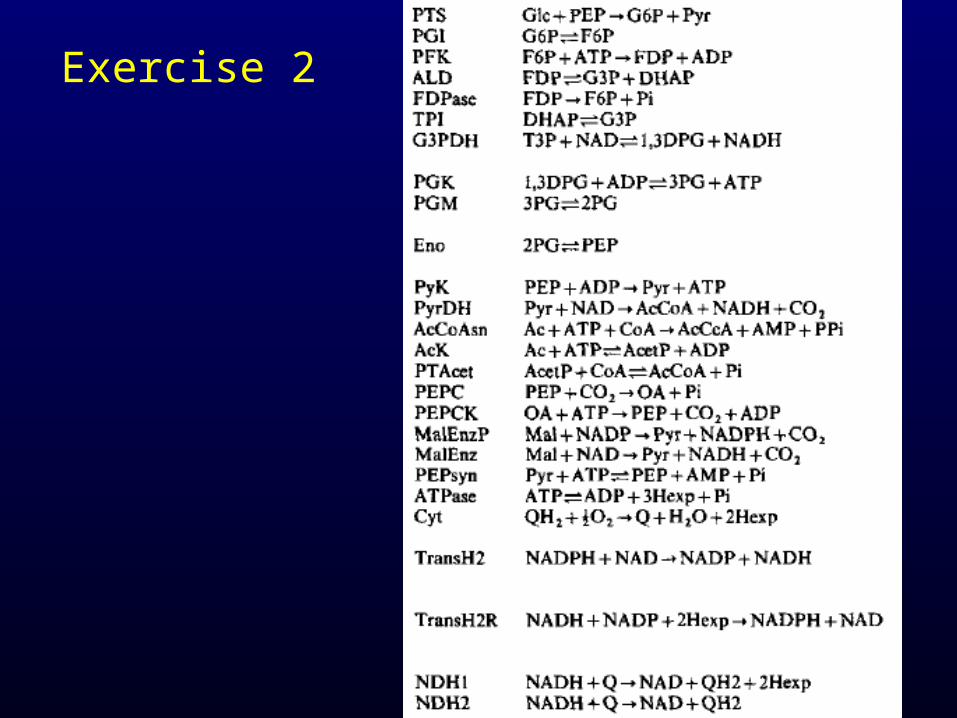
Exercise 2

Topics covered

• Constraint-based approach to metabolic modelling

• Mathematics behind FBA: optimisation

• Mathematical examples

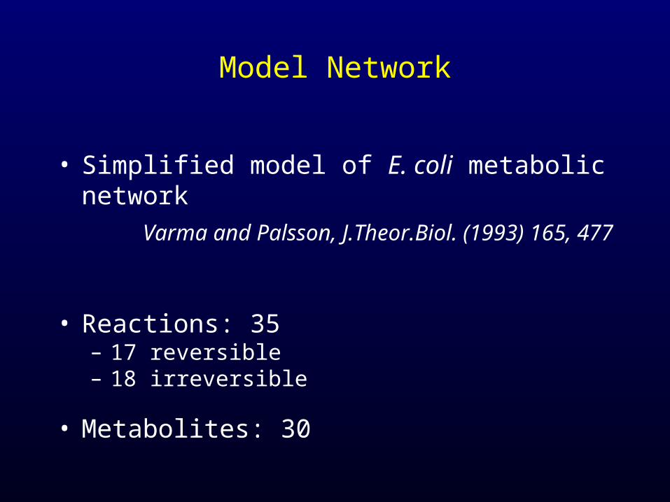
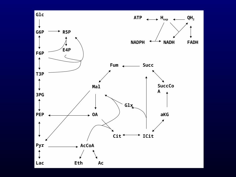
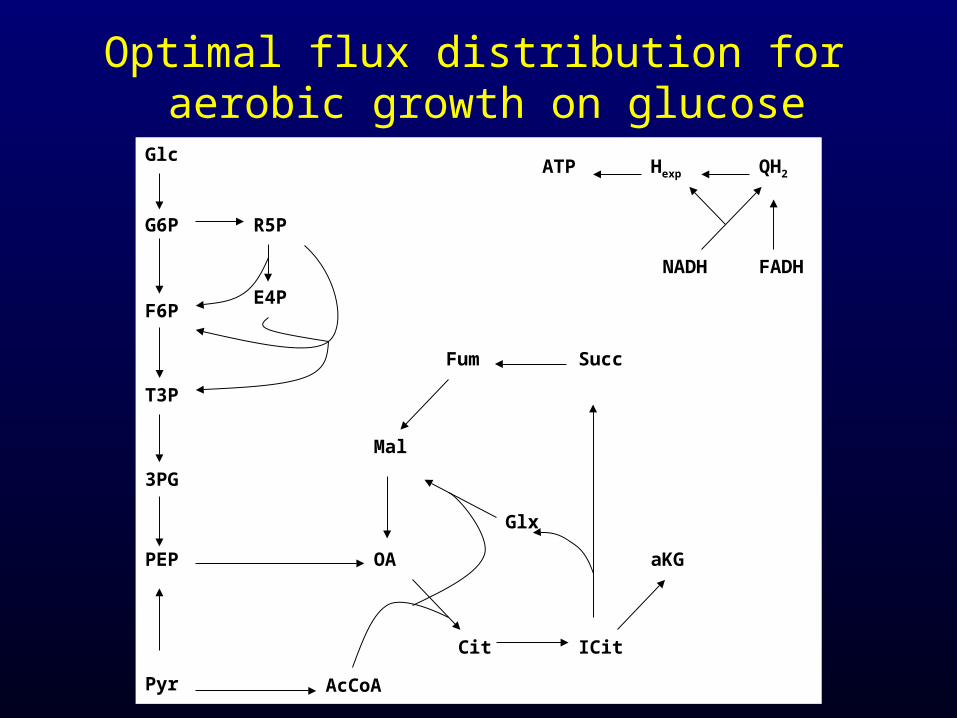
Model Network

• Simplified model of E. coli metabolic network

Varma and Palsson, J.Theor.Biol. (1993) 165, 477

• Reactions: 35– 17 reversible– 18 irreversible

• Metabolites: 30

Glc

Mal

G6P R5P

E4PF6P

T3P

3PG

PEP

Pyr AcCoA

Lac Eth Ac

Cit ICit

aKG

SuccCoA

SuccFum

Glx

OA

NADPH

ATP Hexp QH2

FADHNADH

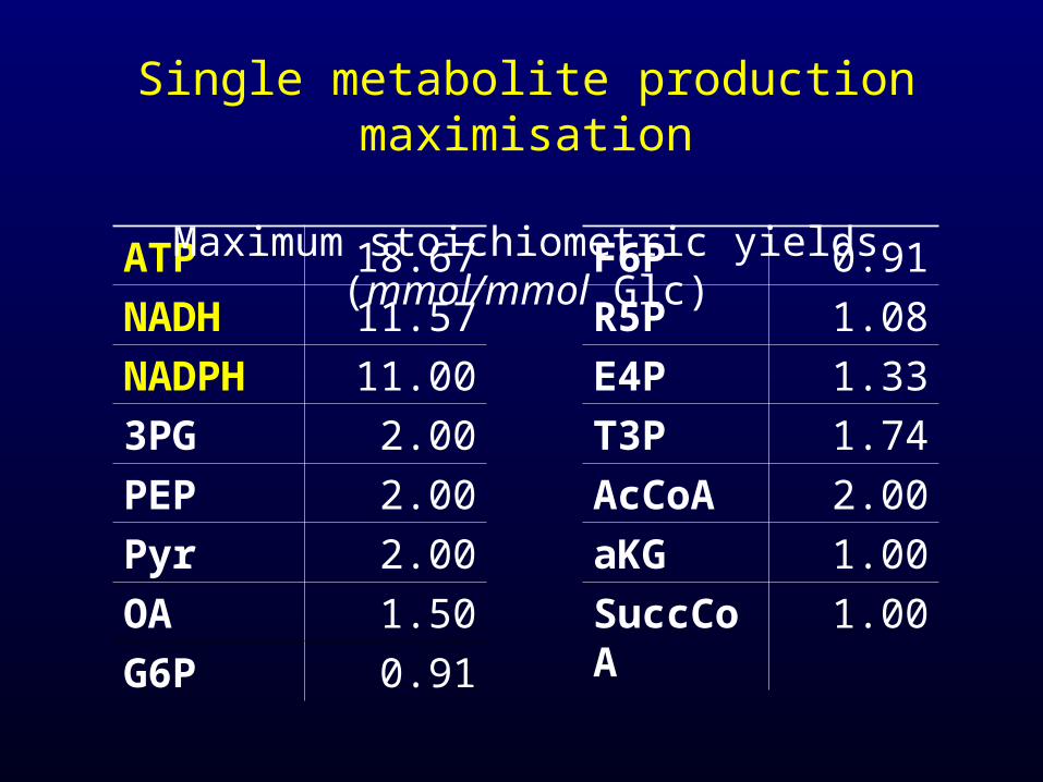
ATP 18.67

NADH 11.57

NADPH 11.00

3PG 2.00

PEP 2.00

Pyr 2.00

OA 1.50

G6P 0.91

F6P 0.91

R5P 1.08

E4P 1.33

T3P 1.74

AcCoA 2.00

aKG 1.00

SuccCoA 1.00

Single metabolite production maximisation

Maximum stoichiometric yields (mmol/mmol Glc)

Glc

Mal

G6P R5P

E4PF6P

T3P

3PG

PEP

Pyr AcCoA

Lac Eth Ac

Cit ICit

aKG

SuccCoA

SuccFum

Glx

OA

NADPH

ATP Hexp QH2

FADHNADH

Glc

Mal

G6P

F6P

T3P

3PG

PEP

Pyr AcCoA

Cit ICit

aKG

SuccCoA

SuccFum

OA

NADPH

ATP Hexp QH2

FADHNADH

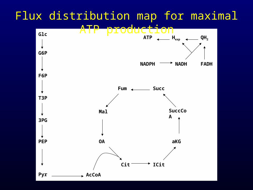
Flux distribution map for maximal ATP production

Glc

Mal

G6P R5P

E4PF6P

T3P

3PG

PEP

Pyr AcCoA

Lac Eth Ac

Cit ICit

aKG

SuccCoA

SuccFum

Glx

OA

NADPH

ATP Hexp QH2

FADHNADH

Glc

Mal

G6P

F6P

T3P

3PG

PEP

Pyr

OA

NADPH

ATP Hexp QH2

NADH

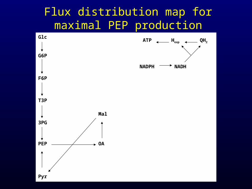
Flux distribution map for maximal PEP production

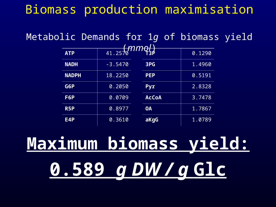
ATP 41.2570

NADH -3.5470

NADPH 18.2250

G6P 0.2050

F6P 0.0709

R5P 0.8977

E4P 0.3610

T3P 0.1290

3PG 1.4960

PEP 0.5191

Pyr 2.8328

AcCoA 3.7478

OA 1.7867

aKgG 1.0789

Biomass production maximisation

Metabolic Demands for 1g of biomass yield (mmol)

Maximum biomass yield:

0.589 g DW / g Glc

Glc

Mal

G6P R5P

E4PF6P

T3P

3PG

PEP

Pyr AcCoA

Lac Eth Ac

Cit ICit

aKG

SuccCoA

SuccFum

Glx

OA

NADPH

ATP Hexp QH2

FADHNADH

Glc

Mal

G6P R5P

E4PF6P

T3P

3PG

PEP

Pyr AcCoA

Cit ICit

aKG

SuccFum

Glx

OA

ATP Hexp QH2

FADHNADH

Optimal flux distribution for aerobic growth on glucose

FBA Summary

• Simple, no kinetic information needed

• Can be applied to large networks

• In accordance with experimental results

• Can be used for defining wider limits of metabolic

behaviour

Further reading

Bernhard O. Palsson: Systems Biology: Properties of reconstructed networks, Cambridge University Press, 2006

Metabolic network reconstruction:Nature Reviews Genetics (2006) 7:130-141.

Metabolic modelling approaches:Journal of Biotechnology (2002) 94: 37-63.Biotechnology and Bioengineering (2003) 84: 763-772

Flux Balance Analysis:Current Opinion in Biotechnology (2003) 14: 491-496.Nature Reviews Microbiology (2004) 2: 886-897

Mathematical programming:Paul Williams: Model Building in Mathematical Programming