
HYDROELASTIC RESPONSE OF SUBMERGED FLOATING TUNNEL
63
HYDROELASTIC RESPONSE OF SUBMERGED FLOATING TUNNEL A Thesis by JIAXING CHEN Submitted to the Office of Graduate and Professional Studies of Texas A&M University in partial fulfillment of the requirements for the degree of MASTER OF SCIENCE Chair of Committee, John Niedzwecki Committee Members, Jeffrey Falzarano Alan Palazzolo Head of Department, Robin Autenrieth December 2015 Major Subject: Ocean Engineering Copyright 2015 Jiaxing Chen
Transcript of HYDROELASTIC RESPONSE OF SUBMERGED FLOATING TUNNEL

HYDROELASTIC RESPONSE OF SUBMERGED FLOATING TUNNEL
A Thesis
by
JIAXING CHEN
Submitted to the Office of Graduate and Professional Studies of
Texas A&M University
in partial fulfillment of the requirements for the degree of
MASTER OF SCIENCE
Chair of Committee, John Niedzwecki
Committee Members, Jeffrey Falzarano
Alan Palazzolo
Head of Department, Robin Autenrieth
December 2015
Major Subject: Ocean Engineering
Copyright 2015 Jiaxing Chen

ii
ABSTRACT
This research investigation addresses the analysis and numerical simulation of
dynamic response of submerged floating tunnels (SFTs) under the influence of surface
waves. As an innovative technical solution for waterway crossings, an SFT is usually
considered as a slender structure restrained by cable system due to its large aspect ratio,
i.e. ratio of length to diameter. Although an SFT is usually placed at a certain depth under
the water surface, it is still susceptible to wave field due to its slenderness. In this research
study, a three-dimensional finite element solving technique, using both Morison’s
equation and modal analysis, is formulated to construct a hydroelastic model of an SFT
and to determine its deformation considering the fluid-structure interactions. Two
preliminary tunnel models for China and Japan, respectively, were studied by
implementing the proposed methodology.
In the first case study, a three-dimensional finite element model of the SFT
prototype in Qiandao Lake (China) was built in Matlab and subsequently analyzed using
mode decomposition to determine its natural frequencies and mode shapes. For each mode
shape, Morison’s equation was employed to calculate fluid forces at each cross section
along the tunnel for given surface wave conditions. Then in the frequency domain, a
complex equation of motion was solved iteratively to address the convergence of the
stiffness of the cable system. The total dynamic response of SFT was the sum of
contributions from each mode component. Results obtained from Matlab were compared
with findings from previous publications and numerical simulations in ABAQUS.

iii
Next, a generic pedestrian-aimed SFT proposed for Otaru Crossing in Japan was
studied. Parametric studies were performed to evaluate the influence of configuration
scheme of cable system and tunnel submerged depth on the dynamic response of SFT.
Results show the importance of fundamental structural parameters in the SFT global
performance and several key conclusions regarding parameter selections were drawn for
engineering practices in design phase.

iv
DEDICATION
To my parents and my wife
For their endless love, support and trust

v
ACKNOWLEDGEMENTS
It has been a wonderful journey for me to study and pursue my Master’s degree in
ocean engineering at Texas A&M University. I would like to express my sincere gratitude
to Prof. John Niedzwecki for his continuous support of my research study and thesis
writing. His patience, motivation, and insightful knowledge has fueled me all the way to
the point where I am today. I would also like to thank Prof. Jeffrey Falzarano for his
suggestions and comments on my research and Prof. Alan Palazzolo for his efforts of
equipping me with solid foundation in finite element analysis.
Besides the aforementioned committee members, I am grateful to Prof. Jun Zhang
and Prof. Moo-Hyun Kim for their dedicated work in teaching wave mechanics and non-
linear hydrodynamics from which I have learnt a lot. Gratitude also goes to other
department faculty and staff for making my time in Aggieland a joyful and memorable
experience. I would also like to thank the Ocean Engineering Program at Texas A&M
University for offering me financial support over the last two years including British
Petroleum Corporation Fellowship and American Bureau of Shipping Scholarship.
In particular, I would like to express my special thanks to Mr. and Mrs. Thompson
(former aggies) for helping me get involved in American culture. I am also grateful to my
wife, Mrs. Bingjie Chen, and all other family members for their selfless love, trust,
patience and support.

vi
NOMENCLATURE
SFT Submerged Floating Tunnel
BEM Boundary Element Method
FEM Finite Element Method
BWR Buoyancy Weight Ratio
K.C. Kuelegan-Carpenter
SIJLAB Sino-Italian Joint Laboratory of Archimedes Bridge
F Hydrodynamic Force
Fluid Density
u Flow Velocity
v Body Velocity
MC Inertia Coefficient
DC Drag Coefficient
V Volume of the Body
A Cross-section Area
maxu Amplitude of the Flow Velocity Oscillation
T Wave Period
L Characteristic Scale of the Object
( , )y x t Structural Response
x Position Variable

vii
t Time Variable
i ith Modal Component
ia Principle Modal Coordinate
U Total Response of SFT
SU Static Response
DU Dynamic Response
M Mass Matrix of the Tunnel
K Stiffness Matrix of the Tunnel
DF Hydrodynamic Force Vector
DU Second Derivative of Dynamic Response w.r.t Time
Natural Frequency
d Mode Shape
D Modal Matrix
( )p t Time Dependent Principle Coordinate Vector
Td Tunnel Diameter
l Length of Each Segment
Tc Cable Axial Force
Inclined Angle
E Young’s Modulus
hK Equivalent Cable Horizontal Stiffness
vK Equivalent Cable Vertical Stiffness

viii
TABLE OF CONTENTS
Page
ABSTRACT .......................................................................................................................ii
DEDICATION .................................................................................................................. iv
ACKNOWLEDGEMENTS ............................................................................................... v
NOMENCLATURE .......................................................................................................... vi
TABLE OF CONTENTS ............................................................................................... viii
LIST OF FIGURES ............................................................................................................ x
LIST OF TABLES ...........................................................................................................xii
1. INTRODUCTION ...................................................................................................... 1
1.1 Overview ............................................................................................................ 1 1.2 Literature Review ............................................................................................... 4
1.3 Research Objectives ........................................................................................... 8
2. METHODOLOGY FORMULATION ....................................................................... 9
2.1 General Morison’s Equation .............................................................................. 9
2.2 Mode Decomposition ....................................................................................... 11 2.3 Hydroelastic Model .......................................................................................... 13
3. IMPLEMENTATION AND VALIDATION ........................................................... 17
3.1 SFT Prototype in Qiandao Lake (PR of China) ............................................... 17 3.1.1 Structural parameters .................................................................................... 18 3.1.2 Fluid properties ............................................................................................. 20
3.2 Sensitivity Study of Cable Stiffness ................................................................. 21 3.3 Numerical Implementation ............................................................................... 24 3.4 Program Validation .......................................................................................... 28
3.4.1 Static calculation .......................................................................................... 28 3.4.2 Dynamic calculation ..................................................................................... 32

ix
Page
4. APPLICATION ........................................................................................................ 37
4.1 Project Description ........................................................................................... 37
4.2 Wave Conditions .............................................................................................. 38 4.3 Structural Model ............................................................................................... 39 4.4 Dynamic Response under Monochromatic Waves .......................................... 40
4.5 Parametric Study .............................................................................................. 44
5. SUMMARY ............................................................................................................. 48
REFERENCES ................................................................................................................. 50

x
LIST OF FIGURES
Page
Figure 1.1 Supporting system of SFT (a) pontoons (b) cables .......................................... 2
Figure 1.2 Illustrations of SFT for (a) transportation (b) recreation ................................. 3
Figure 2.1 Flow past a moving cylinder ............................................................................ 9
Figure 2.2 Illustration of mode decomposition ............................................................... 12
Figure 2.3 Sketch of SFT prototype (Qiandao Lake) in ABAQUS ................................ 14
Figure 3.1 (a) A view of Qiandao Lake (b) Location of the SFT prototype ................... 17
Figure 3.2 Schematic sketch of the SFT prototype ......................................................... 18
Figure 3.3 The cross section of the SFT prototype ......................................................... 19
Figure 3.4 Cable configurations for the SFT prototype .................................................. 19
Figure 3.5 Single-cable system for sensitivity study ....................................................... 21
Figure 3.6 Change of horizontal and vertical stiffness due to tunnel’s movement ......... 23
Figure 3.7 Sketch of SFT (Config. 3) in ABAQUS ........................................................ 25
Figure 3.8 Sketch of SFT model in Matlab ..................................................................... 26
Figure 3.9 Flow chart of stiffness convergence with bisection method .......................... 26
Figure 3.10 Flow chart of numerical analysis in Matlab ................................................. 27
Figure 3.11 Illustration of static force on SFT ................................................................ 29
Figure 3.12 Static results of configuration 1 .................................................................... 29
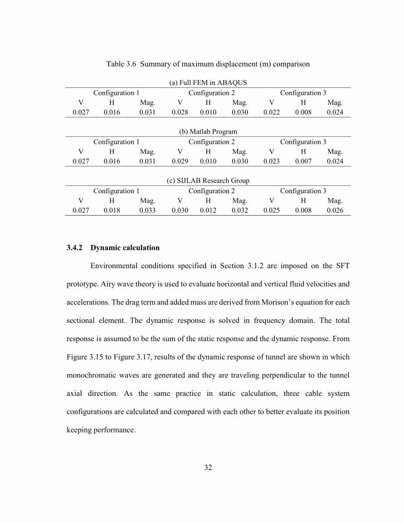
Figure 3.13 Static results of configuration 2 ................................................................... 30
Figure 3.14 Static results of configuration 3 .................................................................... 31
Figure 3.15 Dynamic results of configuration 1 .............................................................. 33

xi
Page
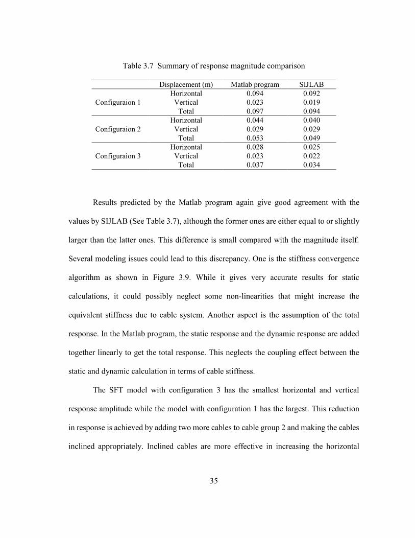
Figure 3.16 Dynamic results of configuration 2 ............................................................. 33
Figure 3.17 Dynamic results of configuration 3 ............................................................. 34
Figure 4.1 Location of Otaru In-port Crossing SFT ........................................................ 38
Figure 4.2 Structural parameters of SFT in Otaru ........................................................... 39
Figure 4.3 Dynamic results of proposed SFT in Otaru ................................................... 40
Figure 4.4 Mode percentage in horizontal response ....................................................... 42
Figure 4.5 Cable group and cable number assignments .................................................. 43
Figure 4.6 Variation of cable tension .............................................................................. 43
Figure 4.7 Comparison of horizontal response ............................................................... 45
Figure 4.8 Comparison of cable tension variations ......................................................... 46

xii
LIST OF TABLES
Page
Table 1.1 Methodologies Comparison on selected papers ................................................ 7
Table 3.1 Equivalent structural parameters of tunnel...................................................... 18
Table 3.2 Structural parameters of cable ......................................................................... 20
Table 3.3 Data of fluid environment ............................................................................... 21
Table 3.4 Cable Properties .............................................................................................. 22
Table 3.5 Cases for Sensitivity Study ............................................................................. 23
Table 3.6 Summary of maximum displacement (m) comparison ................................... 32
Table 3.7 Summary of response magnitude comparison ................................................ 35
Table 4.1 Major feasibility studies done by the society of SFT research in Hokkaido... 37
Table 4.2 Equivalent structural parameters of SFT in Otaru .......................................... 40
Table 4.3 Cases for parametric study .............................................................................. 44

1
1. INTRODUCTION
1.1 Overview
The crossing of waterways has been one of the most complex and challenging
issues in civil engineering. Although hundreds of thousands of conventional structures,
such as suspension bridges and subsea tunnels, have been built successfully around the
world for decades, they have probably reached their maximum level of development and
applications. In addition, many problems and disadvantages have arisen for conventional
solutions when it comes to long crossing distances, deep water areas, complex seabed
morphologies, and severe sea surface conditions. Therefore, a revolutionary solution
needs to be conceived and is required to fulfill the needs of increasingly demanding
crossing conditions.
Submerged floating tunnels (SFTs), an innovative concept emerging in recent
decade, offer the possibility of opening a new chapter of waterway crossings. Unlike
subsea tunnels buried under the seabed, SFTs are usually conceived as tubular floating
structures to be placed at a pre-fixed depth in the water (See Figure 1.1). According to
Archimedes’ principle, the force differential between the total buoyancy and the
gravitational loads results in the net buoyancy that must be counterbalanced by supporting
system distributed along the tunnel. Supporting system can either be pontoons on the
surface or cables anchored to the seabed. With proper design configuration, the tension of
supporting system provides adequate horizontal and vertical stiffness to stabilize the
motions of SFT.

2
(a) (b)
Figure 1.1 Supporting system of SFT (a) pontoons (b) cables [1]
Compared with conventional waterway crossing solutions, SFTs feature the
following four major advantages. First of all, SFTs are designed as modular structures
which makes it stable in every phase of construction and its total cost is approximately
proportional to the whole crossing length.[2] In addition, SFTs with cable anchoring system
have little interference with water surface transportation since the tunnels can be
submerged to create enough clearance depth. Moreover, SFTs can be flexibly applied to
areas with significant changes of seabed slope where subsea tunnel might have difficulty
to be constructed. Finally, as a state-of-the-art design concept, SFTs have less negative
impact on the beauty of the surrounding environment.
Over the last few decades, SFTs have been envisioned for applications such as
vehicle transportation and recreational activities (See Figure 1.2). For SFTs with circular
cross section, diameters can range from 3m to 30m, which is influenced by its design
purposes and the corresponding design loads. As a consequence of the aforementioned
advantages, the length of SFTs can cover a wider range compared with traditional

3
structures. For example, the design length of Daikokujima Crossing SFT (for pedestrian)
is 120m while that of Soya Strait Crossing SFT (for vehicle & railroad) goes up to
43,000m.[3]
(a) (b)
Figure 1.2 Illustrations of SFT for (a) transportation (b) recreation [3]
The aspect ratio of an SFT is defined as the ratio of the tunnel length to its
characteristic cross-section dimension. This ratio can be as large as 102 to 103, which
means an SFT can be treated as a slender beam restrained by cable system that responds
to environmental loadings. Although an SFT is usually submerged at a certain depth in the
water, studies show surface waves still have important influence on its dynamic response
due to its slenderness. Moreover, without the assumption of rigid body behavior, the
interaction between body deformation and surrounding fluid should be taken into
consideration during dynamic analysis.

4
1.2 Literature Review
Since 1980s, there have been comprehensive studies on conceptual design and
dynamic response analysis of SFTs by researchers from Norway, Italy, China, Japan and
Korea. However, no SFT has been constructed at this point. The main reason can be
identified as the consideration of potential uncertainties yet to be discovered and solved.
More and more theoretical and numerical studies, and experimental data are still needed
before the realization of the first SFT construction. In the past decades, the evaluations of
dynamic behavior of SFTs under various environmental conditions, such as waves,
currents, earthquakes, tsunami or accidental loads, have been studied by using theories
and methodologies previously applied to classic floating structures.
Wu (1984)[4], Price et al. (1985)[5], Bishop et al. (1986)[6], and Newman (1994)[7]
presented a generalized three-dimensional hydroelasticity theory to study the fluid-
structure interaction of arbitrary shape objects in wave fields. Their study adopted a
frequency-domain approach, solving for the fluid velocity potential for each mode shape.
This methodology was later employed by Ge et al. (2010)[8] to study the dynamic response
of the SFT prototype in Qiandao Lake (PR of China) under wave effects. Dry mode
components of SFT were calculated using a three-dimensional finite element method. A
boundary element method (BEM) was used to solve for diffraction and radiation
potentials. In order to reduce the computational problems associated with the use of a
three-dimensional BEM, Paik et al. (2004)[9] developed a time-domain dynamic analysis
program for SFTs under wave field. They simplified the problem by pre-calculating added

5
mass and radiation damping coefficients using two-dimensional radiation/diffraction
theory with BEM approach.
Other researchers utilized Morison’s equation for the evaluation of hydrodynamic
forces. Brancaleoni and Castellanit (1989)[10] pursued a coupled fluid-structure interaction
approach incorporating the general Morison’s equation. Lagrangian approach was used to
deal with non-linearity of drag force and the solution was solved via direct time
integration. Using the same methodology, Long el al. (2009)[11] found buoyancy weight
ratio (BWR) and structural damping are two key factors in terms of SFT dynamic
response. With the help of commercial software, Mazzolani et al. (2010)[12] conducted
dynamic analysis via Morison’s equation and they found configurations of cable system
have significant influence on the maximum response amplitude of SFT.
Based upon the aforementioned studies, it can be concluded that there are mainly
two methods for conducting the hydrodynamic analysis of SFTs. One involves using
potential radiation/diffraction theory, and the other is Morison’s equation (See Table 1.1).
According to Kunisu (2010)[13], both methods show pretty good agreement on calculated
wave forces for large K.C. number, in which case it is also recognized that both drag force
and inertia force simultaneously work on SFT.
One advantage of potential theory is that it can be applied within the whole range
of wave frequencies in a sea state. Pressure distribution over SFT surface can be obtained
using Bernoulli’s equation and accurate results can be achieved from discretization using
sufficient boundary elements. However, it’s sometimes very difficult and time consuming
to determine velocity potentials for each mode component and more computational power

6
is needed for large SFTs with long-crossing distances that can be thousands of meters.
Morison’s equation, therefore, can be used under appropriate condition to simplify the
problem. Due to the slenderness of the tunnel, researchers discretize the structure using
finite elements and then calculate the drag and inertia force for each section according to
fluid-structure relative velocity and acceleration at each time step. However, even utilizing
existing commercial software, e.g. ABAQUS[14] or ANSYS, to conduct time-domain
analysis, the computational time grows exponentially as the number of elements increases.
To address these issues, in this research study a different approach combining
Morison’s equation and mode decomposition is pursued. Mode decomposition is used to
identify the dominant modal components for the slender beam. Cable system is modeled
as springs attached to corresponding sections along the beam. Once the mode shapes are
known, Morison’s equation can be applied to calculate fluid forces for each cross section
and then the equation of motion is solved in frequency domain to determine the total
dynamic response of SFT under wave fields.

7
Table 1.1 Methodologies Comparison on selected papers
Author(s) Methodology SFT Dimensions Environmental
Conditions Key Conclusions
Brancaleoni and
Castellanit (1989)
Morison’s equation &
direct time integration &
Lagrangian approach
Elliptic (20x40m)
Length (3000m)
Wave height 6.6m
Wave period 11.2s
Water depth 150m
Spans must be short for severe environments;
Inertia & drag terms significant to response
Long et al. (2009)
Morison’s equation &
frequency-dependent
damping coefficients SFT in Qiandao
Lake
Ciucular (D =
4.39m)
Length (100m)
Wave height 1.0m
Wave period 1.8s
Water depth 30m
Surface current 1.0m/s
Buoyancy weight ratio & structural damping are
key factors in design
Mazzolani,
Faggiano, and
Martire (2010)
Morison’s equation &
ABAQUS/Aqua
package
Three cable system configurations are compared
in terms of displacement, bending moment and
axial force
Ge et al. (2010)
Potential theory with
BEM & mode
decomposition
Without current effect Axial relaxation device could minimize
maximum dynamic reponse
Paik et al. (2004)
2-D diffraction theory
and BEM are employed
to calculate frequency-
dependent parameters.
Impulse response
function is introduced to
solve motion equation.
Circular (D =
11.4m)
Length (855m)
Wave period varies
from 2.25s to 26.46s
Maximum wave height
4.08m
Water depth 100m
SFT submerged depth affects the dynamic
response considerably;
The effect of depth on radiation damping is more
significant than that on added-mass and the
maximum wave force decreases rapidly as SFT
depth increases
Kunisu (2010)
Assume 2-D fixed
structure.
Boundary element
method for diffraction
theory based on the
velocity potential;
Morison’s equation
Circular (D ranges
from 4 to 23m)
Elliptic (23x35m)
Wave number varies
from 0.01 to 0.16
Water depth 100m
Wave force acting on submerged floating tunnel
can be calculated accurately by applying both
Morison’s equation and Boundary Element
Method;
Drag force and inertia force simultaneously
work on the SFT;
Inertia force becomes dominant when K.C. is
less than 15 in the case of SFT with larger
diameter

8
1.3 Research Objectives
The objective of this research study was to formulate a procedure for constructing
a hydroelastic model of a submerged floating tunnel, designed using a three-dimensional
finite element method, and to solve for its dynamic response using a combination of modal
analysis and Morison’s equation in frequency domain. The site specific wave conditions
were modeled as regular waves travelling perpendicular to the longitudinal direction of
the tunnel. The large Kuelegan-Carpenter (K.C.) number for the SFT design allowed the
application of Morison’s equation. Two case studies were conducted as applications of the
proposed methodology. The first case study is based on research data of the SFT prototype
in Qiandao Lake extracted from publications of Sino-Italian Joint Laboratory of
Archimedes Bridge (SIJLAB). The predictions from the new model were compared with
previous findings in terms of maximum static and dynamic response for three different
anchoring system configurations. The second case study deals with a proposed pedestrian-
aimed SFT for the Otaru Crossing project in Japan. Since this proposed SFT has a smaller
diameter compared to transportation applications and is located underwater with
considerable clearance depth, the radiation damping effect can be neglected. In addition,
some parametric studies are conducted to highlight several key structural parameters for
SFT preliminary design.

9
2. METHODOLOGY FORMULATION
2.1 General Morison’s Equation
Flow past a circular cylinder, as shown in Figure 2.1, is a classic problem in ocean
engineering. For incompressible and inviscid potential flow, the total force acting on a
moving body with constant velocity relative to the fluid is zero according to D’Alembert’s
paradox. For inviscid unsteady flow, the hydrodynamic added mass effect is observed as
the surrounding fluid is deflected by the accelerating or decelerating body motion. In
addition to added-mass, drag forces resulting from flow separation and boundary layer
friction should also be taken into consideration in certain cases.
Figure 2.1 Flow past a moving cylinder

10
Morison’s equation was first proposed by Morison, Johnson, and Schaaf (1950)[15]
to describe the hydrodynamic forces on a cylindrical object in an oscillatory flow. For
cases when both the body and fluid are moving, a general Morison’s equation for a body
with unit length is utilized to account for the relative velocity and acceleration.
1
( 1) ( )2
M DF Vu C V u v C A u v u v (2.1)
where is fluid density, u is the flow velocity, v is the body velocity, MC is the inertia
coefficient, DC is the drag coefficient, V is the submerged volume of the body, A is the
cross-sectional area of the body perpendicular to the flow direction.
Later, Keulegan and Carpenter (1956) defined a dimensionless quantity Kc ,
Keulegan-Carpenter number, to describe the relative importance of drag forces over inertia
forces for bluff objects. As a general rule, the inertia component is dominant for 5Kc
while the drag force becomes more important for 15Kc . Kc is written as:
maxu TKc
L (2.2)
where maxu is the amplitude of the flow velocity oscillation, T is the wave period, L is
the characteristic scale of the object in the direction of fluid flow (e.g. the diameter for
cylinder).
One assumption of Morison’s equation for a cylinder in travelling waves is the
diameter of the cylinder is much smaller than the wavelength. This condition limits the
range of wave frequencies that allows the use of Morison’s equation to evaluate wave
forces on the cylinder. According to Vongvisessomjai and Silvester (1976), 5Kc

11
should be satisfied for good estimates by Morison’s equation. For those cases with 5Kc
, the potential radiation/diffraction theory should be pursued instead.
2.2 Mode Decomposition
In structural analysis, mode decomposition is often used for dynamic analysis of
large structural systems. The main idea is the structural motion can be represented by the
sum of a number of mode shapes. In this way, a system with n degrees of freedom (dof)
can be reduced to a simplified model with selected number of dof. This reduction in
dimensionality is extremely important as it simplifies the problem without loss of
significant accuracy and the solving process can be accelerated as it requires less
computational power.
If ( , )y x t is used to represent the exact solution of structural response, x is the
position variable, t is the time variable, ( 1,2,3...)i i is the ith modal component, then
( , )y x t can be approximated as:
1 1 2 2 3 3( , ) ...y x t a a a (2.3)
where 1 2 3, , ...a a a are called principle (modal) coordinates. They are determined by
solving uncoupled equations in terms of selected mode shapes. Theoretically speaking,
the more number of mode shapes selected, the more accurate the result can be. The visual
representation of mode decomposition is shown in Figure 2.2.
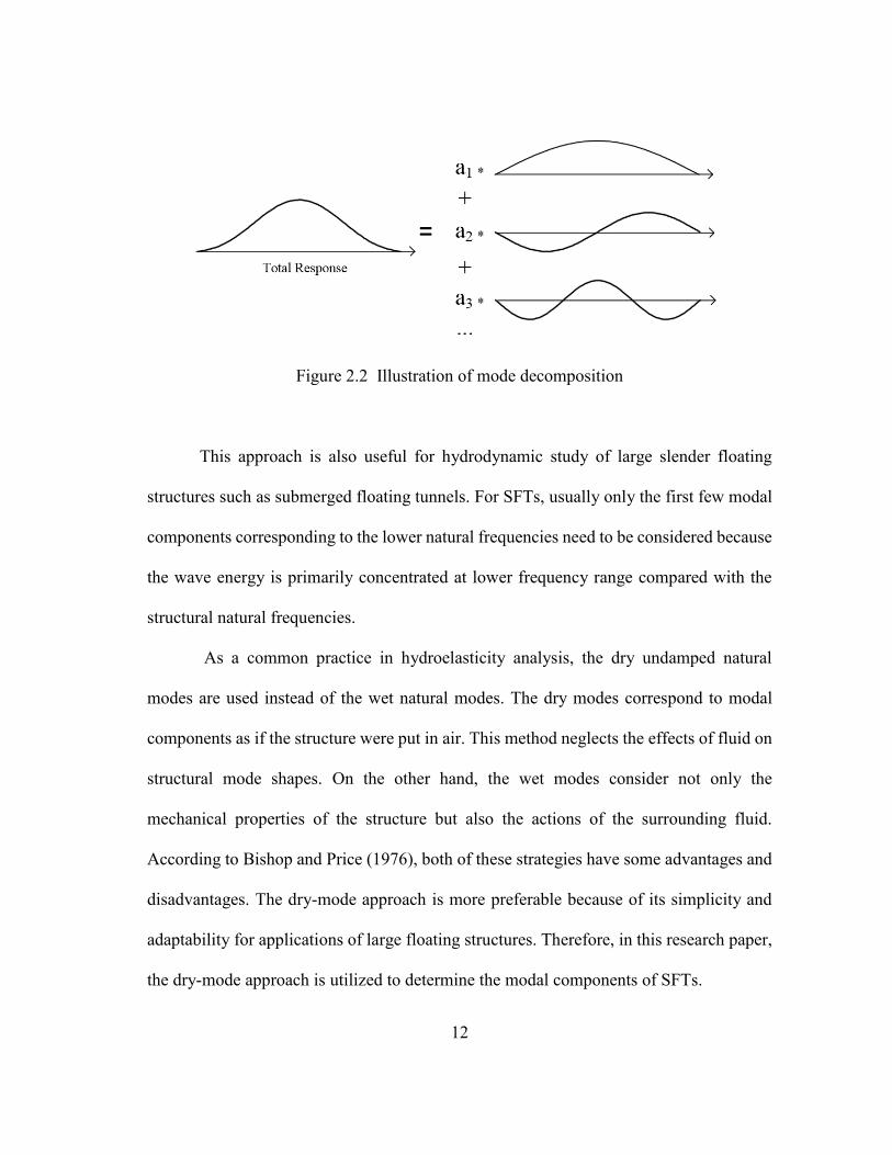
12
Figure 2.2 Illustration of mode decomposition
This approach is also useful for hydrodynamic study of large slender floating
structures such as submerged floating tunnels. For SFTs, usually only the first few modal
components corresponding to the lower natural frequencies need to be considered because
the wave energy is primarily concentrated at lower frequency range compared with the
structural natural frequencies.
As a common practice in hydroelasticity analysis, the dry undamped natural
modes are used instead of the wet natural modes. The dry modes correspond to modal
components as if the structure were put in air. This method neglects the effects of fluid on
structural mode shapes. On the other hand, the wet modes consider not only the
mechanical properties of the structure but also the actions of the surrounding fluid.
According to Bishop and Price (1976), both of these strategies have some advantages and
disadvantages. The dry-mode approach is more preferable because of its simplicity and
adaptability for applications of large floating structures. Therefore, in this research paper,
the dry-mode approach is utilized to determine the modal components of SFTs.

13
2.3 Hydroelastic Model
In this section, the procedure for constructing a hydroelastic model of SFT is
presented based on three-dimensional finite element method (FEM). For environmental
condition, a series of monochromatic waves is travelling perpendicular to the axial
direction of the horizontal SFT. General Morison’s equation is used to calculate wave
forces on slender moving tunnel. The dynamic equation of SFT is decomposed into
uncoupled equations using mode decomposition. The principle modal coordinates are
solved in frequency domain.
The total response U of an SFT is defined as the transverse displacements in
vector form. These displacements are referenced to the straight line connecting the two
ends of the tunnel. U can be estimated as the sum of static response SU and dynamic
response DU .
S DU U U (2.4)
The static response SU is the result of the buoyancy, gravitational loads, and cable
axial loads in still water, which can be easily calculated by Matlab (or ABAQUS) using
fundamental three-dimensional finite element method. The dynamic structural response
DU is a consequence of the hydrodynamic forces induced by the wave field.
14
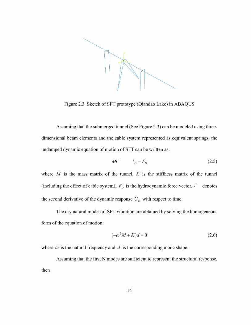
Figure 2.3 Sketch of SFT prototype (Qiandao Lake) in ABAQUS
Assuming that the submerged tunnel (See Figure 2.3) can be modeled using three-
dimensional beam elements and the cable system represented as equivalent springs, the
undamped dynamic equation of motion of SFT can be written as:
D D DMU KU F (2.5)
where M is the mass matrix of the tunnel, K is the stiffness matrix of the tunnel
(including the effect of cable system), DF is the hydrodynamic force vector. DU denotes
the second derivative of the dynamic response DU with respect to time.
The dry natural modes of SFT vibration are obtained by solving the homogeneous
form of the equation of motion:
2( ) 0M K d (2.6)
where is the natural frequency and d is the corresponding mode shape.
Assuming that the first N modes are sufficient to represent the structural response,
then

15
1 2
( )
...
D
N
U D p t
D d d d
(2.7)
where D is the modal matrix containing the first N components, and ( )p t is the time
dependent principle coordinate vector which reflects the magnitude for each natural mode.
When both the tunnel and fluid are moving, the general Morison’s equation is
written as:
2 2
D
1( ) C ( ) 1 ( ) C ( ) ( ) ( ) ( )
4 4 2D M T M T D T D DF t d lu t C d lU t d l u t U t u t U t
(2.8)
where CM is the inertia coefficient and DC is the drag coefficient, is the fluid density
and ( )u t is the fluid velocity, Td is the tunnel diameter and l is the length of each
segment.
Once the SFT is discretized into segments, then for each segment, the general
Morison’s equation is applied. The calculated hydrodynamic force consists of three
components.
e e e e
D inertia added dragF F F F (2.9)
The superscript of e denotes element-wise variant.
It follows then that
D
21
2
1C ( ) ( ) ( ) ( )
2
( )
1
( )
e e e e e e
drag T D D
e ie e i t
e
e e e i t
D
F d l u t U t u t U t
u eu t u eu
U t D p e
(2.10)

16
where ep is a time-independent element-wise principle coordinate vector whose entries
are usually complex values.
Assuming that ( ) ( )Du t U t , which is generally true according to several
research findings, this simplifies the quadratic velocity term in e
dragF as follows:
( ) ( ) ( ) ( )
( ) ( ) ( ) ( ) ( ) ( )
( ) ( ) ( ) ( )
e e e e
D D
e e e e e e
D D D
e e e e
D
u t U t u t U t
u t u t U t U t u t U t
u t u t U t u t
(2.11)
Collecting all the terms and substituting them into the dynamic equation of motion,
the principle coordinate vector p can be determined, and the structural dynamic response
can be evaluated as:
( ) i t
DU t Dpe (2.12)
The total response can then be obtained by adding static response as:
( ) ( )S DU t U U t (2.13)

17
3. IMPLEMENTATION AND VALIDATION
3.1 SFT Prototype in Qiandao Lake (PR of China)
As a case study, the SFT prototype in Qiandao Lake is selected to implement and
validate the proposed methodology (See Figure 3.1). The SFT prototype is an ongoing
project investigated by researchers from the Sino-Italian Joint Laboratory for Archimedes
Bridge (SIJLAB). Since 2004, they have been using both pure Morison’s equation and
potential theory with BEM to determine structural response in the presence of
environmental loadings. Structural dimensions and numerical results are available from
recent publications, which will be discussed in detail in the following sections.
(a) (b)
Figure 3.1 (a) A view of Qiandao Lake (b) Location of the SFT prototype [12]
18
3.1.1 Structural parameters
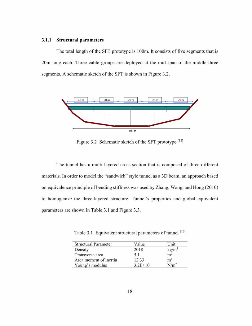
The total length of the SFT prototype is 100m. It consists of five segments that is
20m long each. Three cable groups are deployed at the mid-span of the middle three
segments. A schematic sketch of the SFT is shown in Figure 3.2.
Figure 3.2 Schematic sketch of the SFT prototype [12]
The tunnel has a multi-layered cross section that is composed of three different
materials. In order to model the “sandwich” style tunnel as a 3D beam, an approach based
on equivalence principle of bending stiffness was used by Zhang, Wang, and Hong (2010)
to homogenize the three-layered structure. Tunnel’s properties and global equivalent
parameters are shown in Table 3.1 and Figure 3.3.
Table 3.1 Equivalent structural parameters of tunnel [16]
Structural Parameter Value Unit
Density 2018 kg/m3
Transverse area 5.1 m2
Area moment of inertia 12.33 m4
Young’s modulus 3.2E+10 N/m2
19
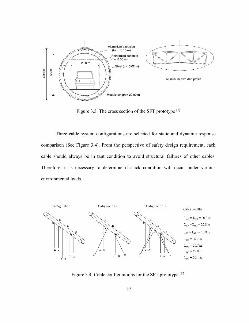
Figure 3.3 The cross section of the SFT prototype [2]
Three cable system configurations are selected for static and dynamic response
comparison (See Figure 3.4). From the perspective of safety design requirement, each
cable should always be in taut condition to avoid structural failures of other cables.
Therefore, it is necessary to determine if slack condition will occur under various
environmental loads.
Figure 3.4 Cable configurations for the SFT prototype [12]

20
Table 3.2 Structural parameters of cable [11]
Structural Parameter Value Unit
Density 7850 kg/m3
Transverse area 2.49E-03 m2
Young’s modulus 3.2E+10 N/m2
Failure load 3140 kN
Design axial load 1045 kN
Inclined angle
OF, QL 0.2 rad
OP, QP 0.4 rad
Others 0 rad
The structural parameters of cables are shown in Table 3.2. The inclined angle of
a cable is defined as the acute angle between the vertical line and the axial direction of the
cable. For cables in group 2 of both configuration 2 and configuration 3, they have
different lengths and inclined angles, which means cable group 2 is an asymmetric
configuration. This asymmetry property results in an unsteady behavior of cable stiffness
which will be discussed in Section 3.2.
3.1.2 Fluid properties
The SFT prototype is placed in the water with a submerged depth of 4.2m. The
clearance depth is 2m which is defined as the distance between the water surface and the
top of the tunnel. The real lake bed profile is uneven as the water depth increases from the
two ends of SFT (10m) to the middle of the inlet (30m). However, a constant depth of
30m in the calculation model is utilized to simplify the problem. Other field data of fluid
properties are given in Table 3.3.
21
Table 3.3 Data of fluid environment [11]
Fluid Parameter Value Unit
Density 1050 kg/m3
Wave height 1 m
Wave period 2.3 s
Surface current velocity 0.1 m/s
Drag coefficient 1 1
Inertia coefficient 2 1
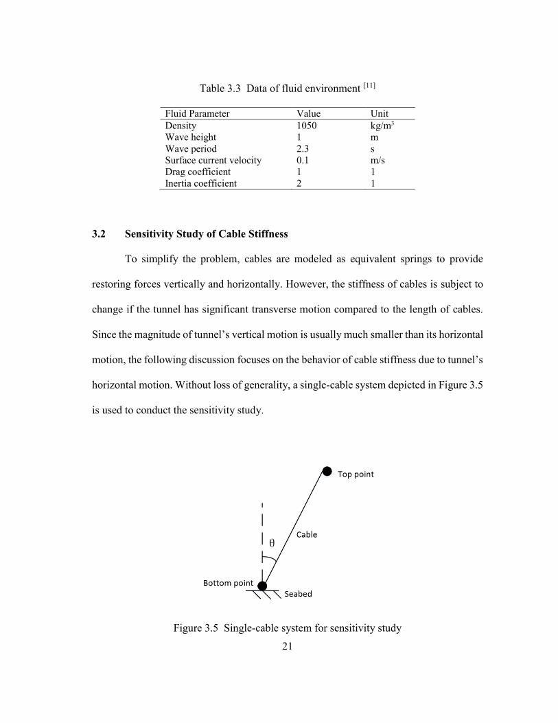
3.2 Sensitivity Study of Cable Stiffness
To simplify the problem, cables are modeled as equivalent springs to provide
restoring forces vertically and horizontally. However, the stiffness of cables is subject to
change if the tunnel has significant transverse motion compared to the length of cables.
Since the magnitude of tunnel’s vertical motion is usually much smaller than its horizontal
motion, the following discussion focuses on the behavior of cable stiffness due to tunnel’s
horizontal motion. Without loss of generality, a single-cable system depicted in Figure 3.5
is used to conduct the sensitivity study.
Figure 3.5 Single-cable system for sensitivity study

22
Table 3.4 Cable Properties
Parameter Value Unit
Diameter 60 mm
Length 30 m
Cross-section area 2.49E-03 m2
Area moment of inertia 6E-07 m4
Young’s modulus 1.4E+11 N/m2
Initial vertical tension component 464.8 kN
Design axial force 1045 kN
Table 3.4 shows the properties of cable in Figure 3.5. The bottom point is anchored
to the seabed. The top point is movable horizontally to simulate the tunnel’s motion. The
initial position of the top point is determined by the static equilibrium position of the tunnel
in still water. The inclined angle is set up with different values to analyze its influence on
stiffness behavior.
The horizontal and vertical stiffness due to the single-cable system are calculated
as follows[17]:
2 2
2 2
cos sin
sin cos
h
v
T EAK
L L
T EAK
L L
(3.1)
where T is the cable axial force, is the inclined angle, E is the Young’s modulus, A
is the cross-section area, L is the length of the cable. Subscripts h and v denote
horizontal and vertical component, respectively.
For better comparison, a constant value of the initial vertical tension component is
imposed on all the cases in Table 3.5.
23
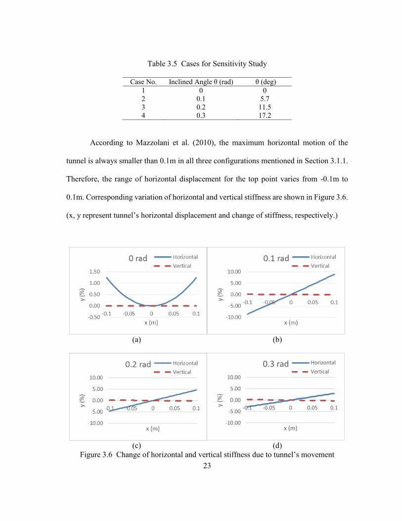
Table 3.5 Cases for Sensitivity Study
Case No. Inclined Angle θ (rad) θ (deg)
1 0 0
2 0.1 5.7
3 0.2 11.5
4 0.3 17.2
According to Mazzolani et al. (2010), the maximum horizontal motion of the
tunnel is always smaller than 0.1m in all three configurations mentioned in Section 3.1.1.
Therefore, the range of horizontal displacement for the top point varies from -0.1m to
0.1m. Corresponding variation of horizontal and vertical stiffness are shown in Figure 3.6.
(x, y represent tunnel’s horizontal displacement and change of stiffness, respectively.)
(a) (b)
(c) (d)
Figure 3.6 Change of horizontal and vertical stiffness due to tunnel’s movement
-10.00
-5.00
0.00
5.00
10.00
-0.1 -0.05 0 0.05 0.1y (%
)
x (m)
0.3 rad Horizontal
Vertical

24
From Figure 3.6, it can be seen that the horizontal stiffness is more sensitive to
tunnel’s horizontal motion compared with the vertical stiffness. When the cable is initially
vertical, its horizontal stiffness follows a parabolic shape due to both positive and negative
displacement. However, as the inclined angle increases, the horizontal stiffness tends to
behave linearly. For vertical stiffness, it does not change a lot in all cases and the variation
is always within ±0.4%.
Furthermore, a conclusion can be drawn for cases with symmetric layout of
inclined cables. If the tunnel transverse motion is small relative to the length of the cables,
the total horizontal stiffness of the cable group can be assumed as a constant due to the
aforementioned linear relationship. For symmetric system with vertical cables, the
horizontal stiffness shows parabolic behavior with its smallest value when the horizontal
displacement is zero. For system with asymmetric cable setup, the horizontal stiffness can
either be linear or nonlinear, which depends on the configuration of each cable and the
amplitude of tunnel motion.
3.3 Numerical Implementation
For each cable system configuration, a three-dimensional finite element model of
the SFT prototype in Qiandao Lake is constructed in Matlab. Also, a corresponding
structural model is built in ABAQUS for comparison with Matlab. Unlike the full finite
element model approach in ABAQUS, cables are transformed into equivalent springs in
the Matlab implementation for each iteration of calculation. This strategy is employed to
accelerate the solving process and is extremely convenient when it comes to parametric

25
study of cable system configurations. A schematic sketch of the SFT prototype with
configuration 3 is shown in Figure 3.7.
Figure 3.7 Sketch of SFT (Config. 3) in ABAQUS
In ABAQUS, the two ends of the tunnel have different boundary conditions. The
upper left end is modeled as a hinge with free rotation while the lower right end has an
additional degree of freedom in the axial direction of the tunnel. For cables, all the bottom
anchored points and top points are also modeled as hinges. Joint connectors are created to
ensure all top cable points are following the corresponding sectional displacements of the
tunnel. The tunnel is meshed with 3-node quadratic beam elements and each cable is
modeled as a 2-node linear truss element.
In Matlab, the tunnel is discretized into 2-node linear beam elements. With
convergence tests conducted, the element size is set to be 1m and hence the total number
of beam elements is 100. Each configuration has three cable groups. A cable group can be
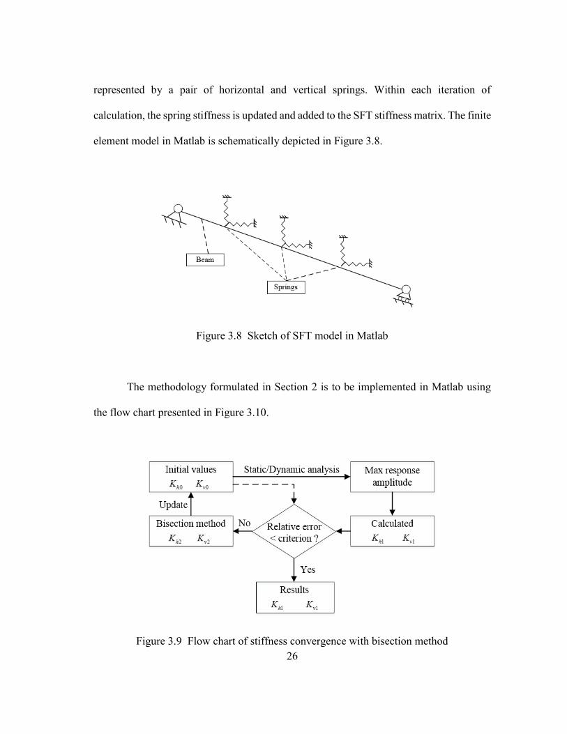
26
represented by a pair of horizontal and vertical springs. Within each iteration of
calculation, the spring stiffness is updated and added to the SFT stiffness matrix. The finite
element model in Matlab is schematically depicted in Figure 3.8.
Figure 3.8 Sketch of SFT model in Matlab
The methodology formulated in Section 2 is to be implemented in Matlab using
the flow chart presented in Figure 3.10.
Figure 3.9 Flow chart of stiffness convergence with bisection method

27
Figure 3.10 Flow chart of numerical analysis in Matlab
For both static and dynamic calculations, a bisection method is introduced to
repeatedly capture the variation of cable stiffness and to obtain an approximate solution.
This method starts from the initial condition of SFT under still water. Each cable group
has a set of equivalent initial horizontal and vertical stiffness denoted as 0hK and 0vK ,
respectively. These stiffness are used to determine the response of SFT under
environmental loads. Once the response amplitude is known, the corresponding horizontal
and vertical stiffness of each cable group, denoted 1hK and 1vK , are calculated and
compared to 0hK and 0vK . If the difference does not satisfy the specified convergence
criterion, 2hK and 2vK will be determined based on the mean position of the previous two

28
results, and will replace 0hK and 0vK as the new initial values for the next iteration. Loops
of calculation are executed until the relative error is sufficiently small. See Figure 3.9 for
stiffness convergence and Figure 3.10 for Matlab implementation.
3.4 Program Validation
Both static and dynamic analyses of the SFT prototype are conducted in the Matlab
program and the results are compared with full FEM in ABAQUS and publications from
SIJLAB[12]. Three cable system configurations (refer to Figure 3.4) are also compared in
terms of maximum structural response. Finally, maximum cable axial forces are
determined to assess the performance of cable system.
3.4.1 Static calculation
For static cases, drag and inertia components due to both current and waves are
evaluated as “static” values. The resultant horizontal and vertical hydrodynamic forces are
4.875 kN/m and 4.860 kN/m, respectively. Besides, buoyancy and gravitational loads are
also added to the vertical component. The sketch of forces acting on the SFT with
configuration 3 is shown in Figure 3.11.
29
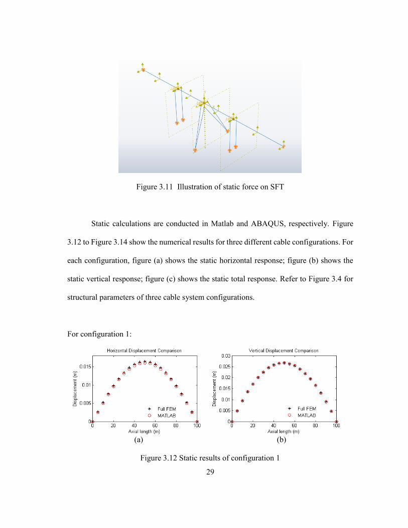
Figure 3.11 Illustration of static force on SFT
Static calculations are conducted in Matlab and ABAQUS, respectively. Figure
3.12 to Figure 3.14 show the numerical results for three different cable configurations. For
each configuration, figure (a) shows the static horizontal response; figure (b) shows the
static vertical response; figure (c) shows the static total response. Refer to Figure 3.4 for
structural parameters of three cable system configurations.
For configuration 1:
(a) (b)
Figure 3.12 Static results of configuration 1
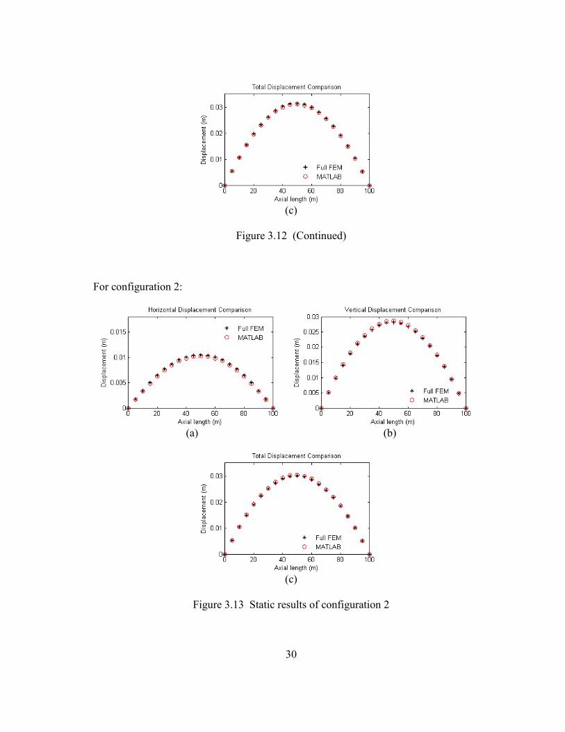
30
(c)
Figure 3.12 (Continued)
For configuration 2:
(a) (b)
(c)
Figure 3.13 Static results of configuration 2

31
For configuration 3:
(a) (b)
(c)
Figure 3.14 Static results of configuration 3
In Table 3.6, “V” denotes vertical, “H” denotes horizontal, and “Mag.” denotes
total magnitude. Results of displacements under static loads from the Matlab program
show pretty good agreement with those obtained by full FEM in ABAQUS. Although little
discrepancy is observed between the Matlab program and the SIJLAB research group, this
error is expected and acceptable because a simplified model was used in the former
approach. In addition, selections of different types of beam elements and meshing density
can also contribute to the variation in the results.
32
Table 3.6 Summary of maximum displacement (m) comparison
(a) Full FEM in ABAQUS
Configuration 1 Configuration 2 Configuration 3
V H Mag. V H Mag. V H Mag.
0.027 0.016 0.031 0.028 0.010 0.030 0.022 0.008 0.024
(b) Matlab Program
Configuration 1 Configuration 2 Configuration 3
V H Mag. V H Mag. V H Mag.
0.027 0.016 0.031 0.029 0.010 0.030 0.023 0.007 0.024
(c) SIJLAB Research Group
Configuration 1 Configuration 2 Configuration 3
V H Mag. V H Mag. V H Mag.
0.027 0.018 0.033 0.030 0.012 0.032 0.025 0.008 0.026
3.4.2 Dynamic calculation
Environmental conditions specified in Section 3.1.2 are imposed on the SFT
prototype. Airy wave theory is used to evaluate horizontal and vertical fluid velocities and
accelerations. The drag term and added mass are derived from Morison’s equation for each
sectional element. The dynamic response is solved in frequency domain. The total
response is assumed to be the sum of the static response and the dynamic response. From
Figure 3.15 to Figure 3.17, results of the dynamic response of tunnel are shown in which
monochromatic waves are generated and they are traveling perpendicular to the tunnel
axial direction. As the same practice in static calculation, three cable system
configurations are calculated and compared with each other to better evaluate its position
keeping performance.
33
For configuration 1:
(a) (b)
(c)
Figure 3.15 Dynamic results of configuration 1
For configuration 2:
(a) (b)
Figure 3.16 Dynamic results of configuration 2

34
(c)
Figure 3.16 (Continued)
For configuration 3:
(a) (b)
(c)
Figure 3.17 Dynamic results of configuration 3
35
Table 3.7 Summary of response magnitude comparison
Displacement (m) Matlab program SIJLAB
Configuraion 1
Horizontal 0.094 0.092
Vertical 0.023 0.019
Total 0.097 0.094
Configuraion 2
Horizontal 0.044 0.040
Vertical 0.029 0.029
Total 0.053 0.049
Configuraion 3
Horizontal 0.028 0.025
Vertical 0.023 0.022
Total 0.037 0.034
Results predicted by the Matlab program again give good agreement with the
values by SIJLAB (See Table 3.7), although the former ones are either equal to or slightly
larger than the latter ones. This difference is small compared with the magnitude itself.
Several modeling issues could lead to this discrepancy. One is the stiffness convergence
algorithm as shown in Figure 3.9. While it gives very accurate results for static
calculations, it could possibly neglect some non-linearities that might increase the
equivalent stiffness due to cable system. Another aspect is the assumption of the total
response. In the Matlab program, the static response and the dynamic response are added
together linearly to get the total response. This neglects the coupling effect between the
static and dynamic calculation in terms of cable stiffness.
The SFT model with configuration 3 has the smallest horizontal and vertical
response amplitude while the model with configuration 1 has the largest. This reduction
in response is achieved by adding two more cables to cable group 2 and making the cables
inclined appropriately. Inclined cables are more effective in increasing the horizontal

36
stiffness of SFT. For example, the equivalent horizontal stiffness for cable group 2 in
configuration 1 is 2.94E+04 N/m while that in configuration 3 is 9.66E+06 N/m.
From Table 3.6 and Table 3.7, it can also be observed that the response amplitudes
are much larger in dynamic calculations than in static calculations. The reason lies in the
fact that the structural acceleration was not taken into account in static cases. Since the
added mass coefficient is 1, the fluid forces generated by the tunnel’s motion can increase
the total force significantly when the relative acceleration is larger than the amplitude of
the fluid acceleration itself. Therefore, it is undoubtedly necessary to conduct dynamic
analyses of SFTs as oppose to static calculations because static predictions would
generally underestimate the forces and hence displacements.

37
4. APPLICATION
4.1 Project Description
Over the past 20 years, the society of SFT research in Hokkaido has carried out a
variety of feasibility studies of various SFT projects in Japan from numerical simulations
to experiments. These proposed applications cover a wide range of design purposes,
crossing distances, and water depths. See Table 4.1.
Table 4.1 Major feasibility studies done by the society of SFT research in Hokkaido [3]
Name Location Purpose Length
(m)
Max.Water
Depth (m)
Funka Bay Crossing Bay threshold Motor vehicle
Railroad
30,000 120
Toya Lake Crossing Lake crossing Pedestrian
Mono-rail
3,000 100
Rishiri Rebun Crossing Strait Crossing Lifeline
Transportation
22,000 200
Ishikariwan Shinko In-port
Crossing
In-port Crossing Motor vehicle 972 15
Daikokujima Crossing In-port Crossing Pedestrian 120 10
Soya Strait Crossing Strait Crossing Motor vehicle
Railroad
43,000 180
Otaru In-port Crossing In-port Crossing Pedestrian 300 10
The Otaru In-port Crossing project is specifically selected as the application of the
methodology developed in Chapter 2 for two reasons. First, it is a pedestrian-aimed SFT
with a crossing distance of 300m, which is longer than the SFT prototype in Qiandao Lake.
The characteristic of slenderness is more dominant in this case with larger aspect ratio.
Second, it is located in a relatively shallow water region with maximum water depth of

38
10m. The horizontal motion of the SFT is more vulnerable to surface waves due to the
elliptical water particle trajectories throughout the water column. Conversely the water
depth of the Qiandao Lake is 30m. In this case surface waves have less influence if the
SFT is submerged deep enough in the water.
(a) (b)
Figure 4.1 Location of Otaru In-port Crossing SFT
4.2 Wave Conditions
According to the wave statistics provided by Windfinder[18], the typical wave
height and wave length in service condition are 0.9m and 22m, respectively. Because the
axial direction of the SFT is approximately parallel to the shoreline (See Figure 4.1), it is
assumed that waves are travelling perpendicular to the longitudinal direction of the tunnel.
39
4.3 Structural Model
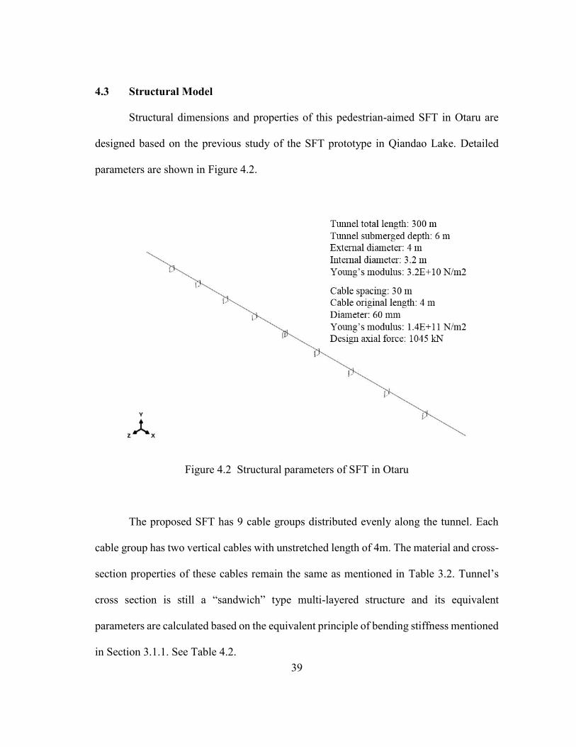
Structural dimensions and properties of this pedestrian-aimed SFT in Otaru are
designed based on the previous study of the SFT prototype in Qiandao Lake. Detailed
parameters are shown in Figure 4.2.
Figure 4.2 Structural parameters of SFT in Otaru
The proposed SFT has 9 cable groups distributed evenly along the tunnel. Each
cable group has two vertical cables with unstretched length of 4m. The material and cross-
section properties of these cables remain the same as mentioned in Table 3.2. Tunnel’s
cross section is still a “sandwich” type multi-layered structure and its equivalent
parameters are calculated based on the equivalent principle of bending stiffness mentioned
in Section 3.1.1. See Table 4.2.

40
Table 4.2 Equivalent structural parameters of SFT in Otaru
Structural Parameter Value Unit
Density (with live loads) 2200 kg/m3
Transverse area 4.5 m2
Area moment of inertia 7.42 m4
Young’s modulus 3.2E+10 N/m2
The tunnel is discretized into 2-node linear beam elements. The element size is set
to 3m after convergence tests. All cables are modeled as springs with initial stiffness
values obtained from results in still water. One end of the tunnel is a hinge connection and
the other end has an axial relaxation device.
4.4 Dynamic Response under Monochromatic Waves
The three-dimensional finite element model of the SFT and the monochromatic
waves specified in Section 4.2 are simulated in the Matlab program. The results of static,
dynamic, and total response are shown in Figure 4.3.
(a) (b)
Figure 4.3 Dynamic results of proposed SFT in Otaru

41
(c)
Figure 4.3 (Continued)
The total horizontal response is much larger than the total vertical response. The
amplitude of the vertical response is only 5.7% of the horizontal response. The vertical
response is restrained to a small value (0.007m) by the presence of cables distributed along
the tunnel. From Section 3.2, it is observed that a vertical cable provides less horizontal
stiffness to the tunnel than an inclined cable. This is generally true if the horizontal motion
of the SFT is negligible compared to the length of the cable. In the case of Otaru SFT, the
length of cables is restricted by the 10m water depth. The effects of short inclined cables
on the SFT behavior is of great interest and will be investigated in Section 4.5.
Since the dynamic response is calculated based upon the contributions from
selected modes, it is important to determine whether enough mode components have been
selected to well represent the SFT behavior. As stated in Equation (2.10) in Section 2.3,
ep is a vector whose magnitude reflects the contribution from each mode. With that
determined from previous calculation, the percentage that each mode accounts for in the
total horizontal response can be shown in Figure 4.4.
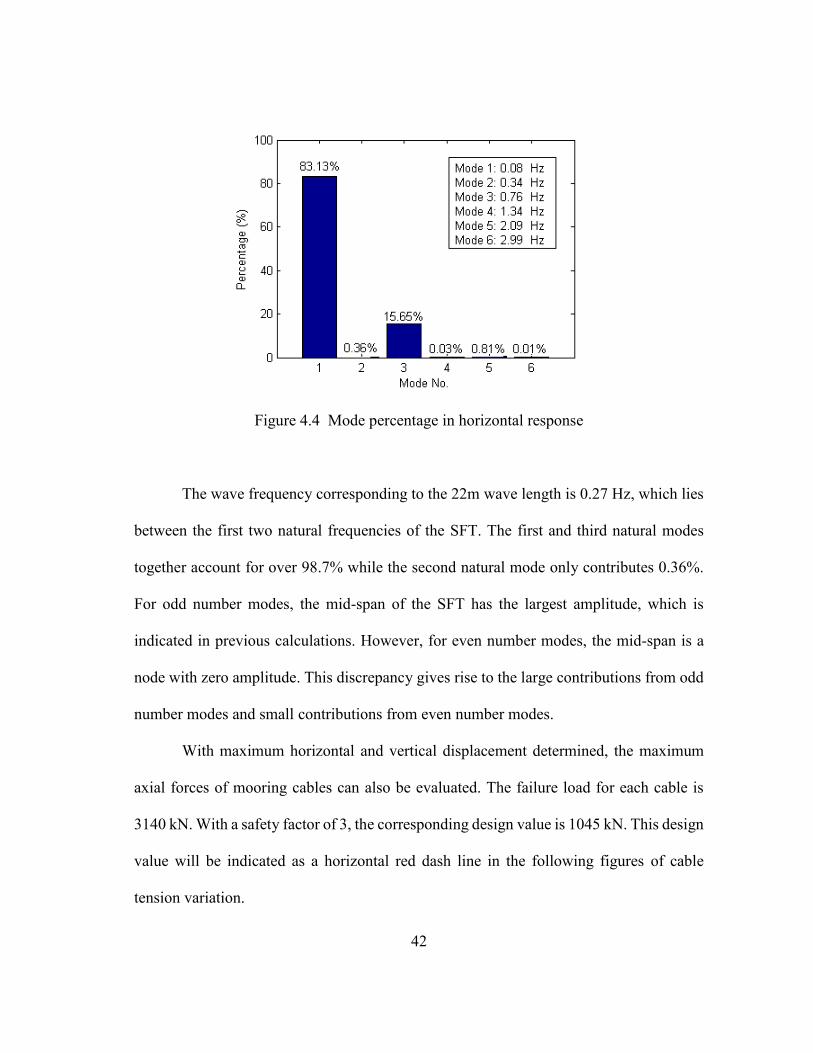
42
Figure 4.4 Mode percentage in horizontal response
The wave frequency corresponding to the 22m wave length is 0.27 Hz, which lies
between the first two natural frequencies of the SFT. The first and third natural modes
together account for over 98.7% while the second natural mode only contributes 0.36%.
For odd number modes, the mid-span of the SFT has the largest amplitude, which is
indicated in previous calculations. However, for even number modes, the mid-span is a
node with zero amplitude. This discrepancy gives rise to the large contributions from odd
number modes and small contributions from even number modes.
With maximum horizontal and vertical displacement determined, the maximum
axial forces of mooring cables can also be evaluated. The failure load for each cable is
3140 kN. With a safety factor of 3, the corresponding design value is 1045 kN. This design
value will be indicated as a horizontal red dash line in the following figures of cable
tension variation.

43
Figure 4.5 Cable group and cable number assignments
Figure 4.6 Variation of cable tension
Figure 4.5 shows the cable and cable group numbering for the Otaru SFT. In Figure
4.6, the white bars indicate the cable tension in still water and the solid bars represent the
maximum cable tension under surface waves. Attention should be given to cables
44
distributed around the mid-span of SFT. These cables have the largest displacement and
therefore, variation compared with those near the two ends. The maximum tension
occurring at Cable No.9 and No.10 is about 62% of the design value (1045 kN), which is
high as the cables might have larger tension variation as the SFT undergoes more severe
environmental conditions. More cables and better configuration scheme are needed to
enhance the structural integrity of the SFT.
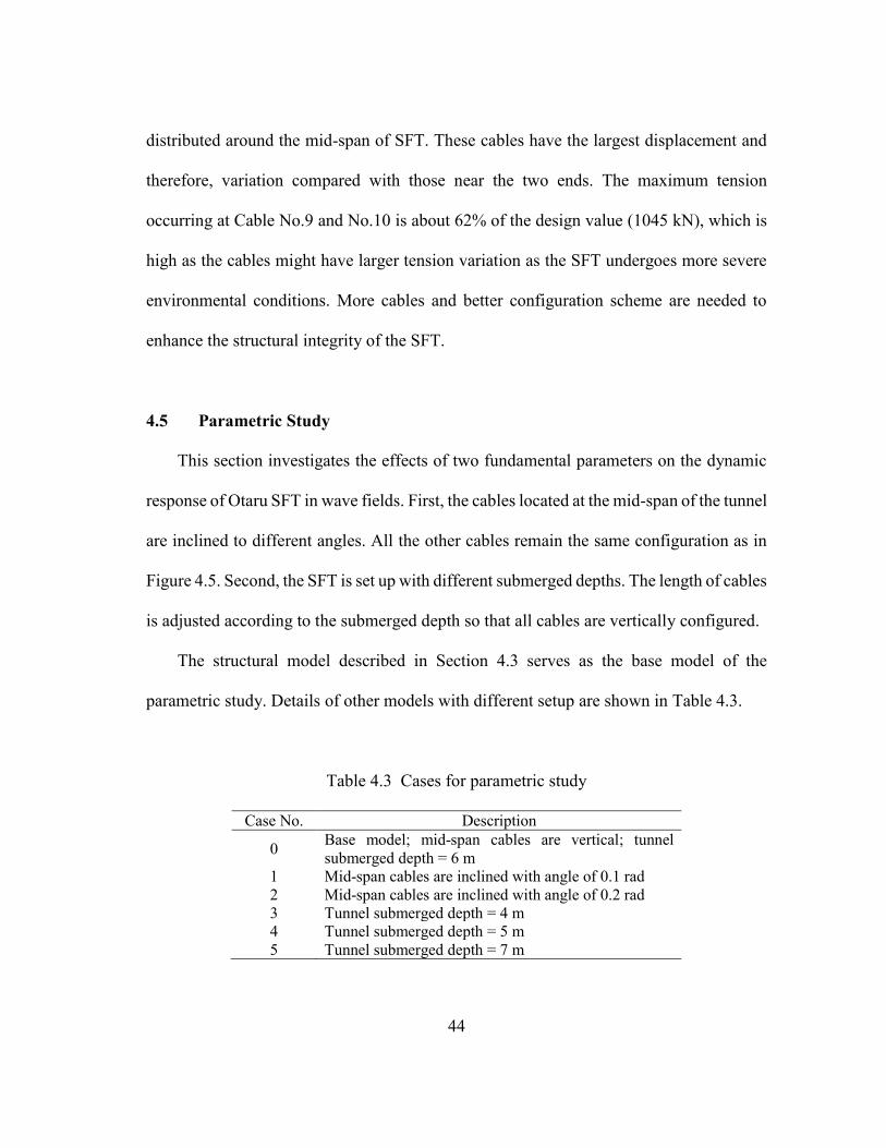
4.5 Parametric Study
This section investigates the effects of two fundamental parameters on the dynamic
response of Otaru SFT in wave fields. First, the cables located at the mid-span of the tunnel
are inclined to different angles. All the other cables remain the same configuration as in
Figure 4.5. Second, the SFT is set up with different submerged depths. The length of cables
is adjusted according to the submerged depth so that all cables are vertically configured.
The structural model described in Section 4.3 serves as the base model of the
parametric study. Details of other models with different setup are shown in Table 4.3.
Table 4.3 Cases for parametric study
Case No. Description
0 Base model; mid-span cables are vertical; tunnel
submerged depth = 6 m
1 Mid-span cables are inclined with angle of 0.1 rad
2 Mid-span cables are inclined with angle of 0.2 rad
3 Tunnel submerged depth = 4 m
4 Tunnel submerged depth = 5 m
5 Tunnel submerged depth = 7 m

45
All cases are simulated in the Matlab program with the same surface wave condition
given in Section 4.2. The horizontal response and cable tension variation are compared
and shown as follows.
Figure 4.7 Comparison of horizontal response

46
It is observed in Table 3.7 that inclined cables can provide larger horizontal stiffness
to SFTs compared to vertical cables. However, in Figure 4.7 (a), for inclined angle
configuration, the horizontal response amplitude along the tunnel is larger than base case.
The underlying reason is the presence of slack cables, which is illustrated in Figure 4.8.
From Figure 4.7 (b), it is obvious that the influence of the submerged depth on the
horizontal response of SFT is significant. There are two main reasons. First, as the SFT
gets closer to the water surface, the larger the hydrodynamic forces become. Second,
provided the tension of each cable remains the same, the longer the vertical cable, the
lesser horizontal stiffness it can offer according to Equation (3.1).
Figure 4.8 Comparison of cable tension variations
47
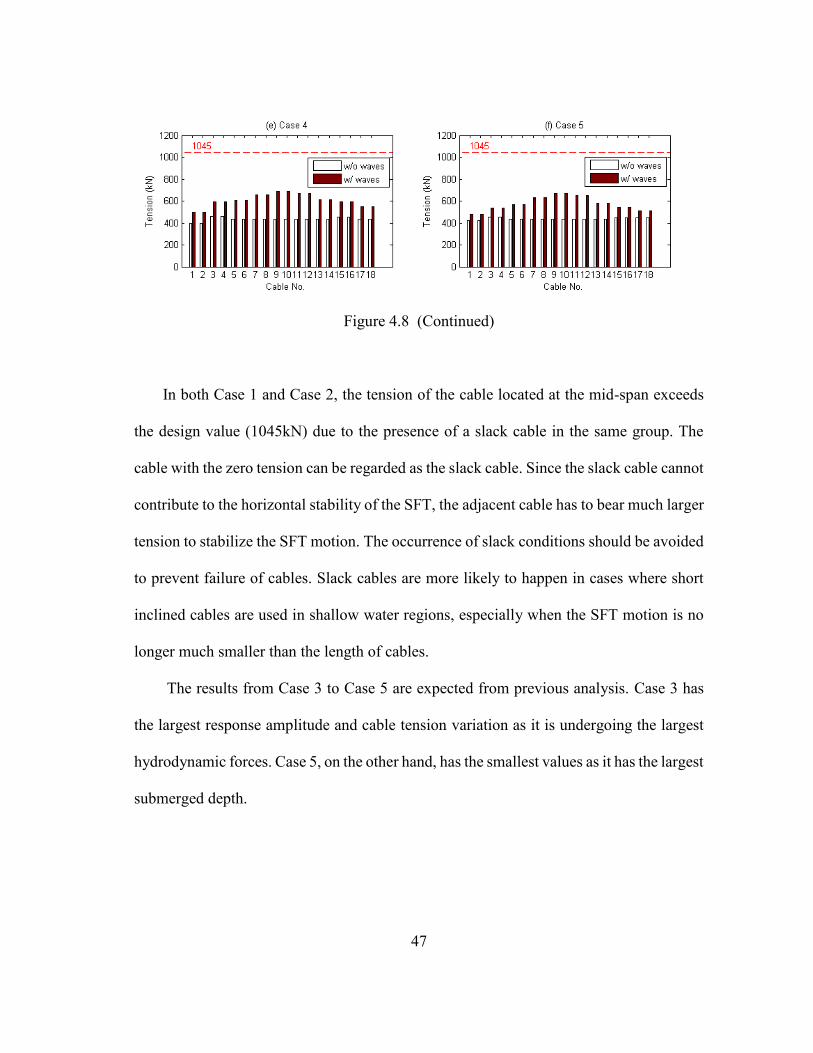
Figure 4.8 (Continued)
In both Case 1 and Case 2, the tension of the cable located at the mid-span exceeds
the design value (1045kN) due to the presence of a slack cable in the same group. The
cable with the zero tension can be regarded as the slack cable. Since the slack cable cannot
contribute to the horizontal stability of the SFT, the adjacent cable has to bear much larger
tension to stabilize the SFT motion. The occurrence of slack conditions should be avoided
to prevent failure of cables. Slack cables are more likely to happen in cases where short
inclined cables are used in shallow water regions, especially when the SFT motion is no
longer much smaller than the length of cables.
The results from Case 3 to Case 5 are expected from previous analysis. Case 3 has
the largest response amplitude and cable tension variation as it is undergoing the largest
hydrodynamic forces. Case 5, on the other hand, has the smallest values as it has the largest
submerged depth.

48
5. SUMMARY
Although the evaluations of wave forces on submerged floating tunnels (SFTs)
have been studied for many years, a computationally efficient and robust solving
technique is still needed for initial investigation of anchoring system performance and
structural parametric study. With this aim, a frequency-domain approach utilizing both the
Morison’s equation and mode decomposition was proposed in this research investigation.
The main objective of this research study was to formulate the procedure of building
hydroelastic model of SFTs and to validate the proposed methodology.
In order to analyze the hydrodynamic behavior of the SFT prototype under
monochromatic surface waves in Qiandao Lake, a three-dimensional finite element
hydroelastic model was first constructed. In this model, linear beam elements were
adopted to mimic the slender behavior of the tunnel. The anchoring system was
represented by horizontal and vertical springs with equivalent stiffness. A sensitivity study
of cable stiffness was performed to better understand the influence of tunnel’s motion.
Results showed horizontal stiffness was more sensitive and its value was also affected by
the cable’s inclined angle. As part of the numerical program, a bisection method was
introduced to guarantee and accelerate the convergence of stiffness calculations. Both
static and dynamic predictions by the proposed methodology showed good agreement with
results from SIJLAB in terms of horizontal and vertical response amplitude.
The methodology developed in this study was further applied to investigate the
structural response of the Otaru In-port crossing SFT. In this design, all of the anchoring

49
lines were vertical and evenly distributed along the length of the 300m long tunnel. The
total response of the tunnel under service wave conditions provided by Windfinder was
obtained by summing the static and dynamic response contributions. For the safety
requirement, the maximum axial force for each anchoring line was calculated with respect
to the total response amplitude. Contributions of different modal components to the total
response were also determined in order to check whether adequate mode shapes had been
selected. Parametric studies based on this generic model were conducted in terms of cable
inclined angle and tunnel submerged depth. As the tunnel gets closer to the water surface,
the SFT undergoes increasing hydrodynamic forces as expected. Results also suggest in
shallow water areas where cable length is confined to a small value, inclined cable
configurations should be used with caution as slack conditions might happen which leads
to high tension and failure to adjacent anchoring lines.
In summary, the proposed hydroelastic model and methodology can well predict
the dynamic response of SFTs under monochromatic waves. It provides a fast and accurate
approach to analyze the hydroelasticity of SFTs from the perspective of modal analysis.
As a computationally efficient procedure, it possesses great advantages in terms of global
anchoring system selection and structural parametric study. As part of the future work,
this methodology will be extended to irregular waves by using linear system approach.
Spectral analysis can then be implemented to evaluate the dynamic response of SFTs in
frequency domain. In addition, the effects of current and structural radiation should be
taken into account for better predictions of structural response in various environmental
conditions.

50
REFERENCES
[1] B. Jakobsen, “Design of the Submerged Floating Tunnel operating under various
conditions,” Procedia Eng., vol. 4, no. 1877, pp. 71–79, Jan. 2010.
[2] F. M. Mazzolani, R. Landolfo, B. Faggiano, M. Esposto, F. Perotti, and G.
Barbella, “Structural Analyses of the Submerged Floating Tunnel Prototype in
Qiandao Lake (PR of China),” Adv. Struct. Eng., vol. 11, no. 4, pp. 439–454, Aug.
2008.
[3] S. Kanie, “Feasibility studies on various SFT in Japan and their technological
evaluation,” Procedia Eng., vol. 4, pp. 13–20, 2010.
[4] Y. Wu, “Hydroelasticity of floating bodies.” University of Brunel, London, UK,
1984.
[5] W. G. Price and Y. Wu, “Hydroelasticity Of Marine Structures,” Cambridge
University Press, Cambridge, UK, 1986.
[6] R. E. D. Bishop, W. G. Price, and Y. Wu, “A General Linear Hydroelasticity
Theory of Floating Structures Moving in a Seaway,” Philos. Trans. R. Soc. A
Math. Phys. Eng. Sci., vol. 316, no. 1538, pp. 375–426, Apr. 1986.
[7] J. N. Newman, “Wave effects on deformable bodies,” Appl. Ocean Res., vol. 16,
no. 1, pp. 47–59, Jan. 1994.
[8] F. Ge, W. Lu, X. Wu, and Y. Hong, “Fluid-structure interaction of submerged
floating tunnel in wave field,” Procedia Eng., vol. 4, pp. 263–271, Jan. 2010.
[9] I. Y. Paik, C. K. Oh, J. S. Kwon, and S. P. Chang, “Analysis of wave force
induced dynamic response of submerged floating tunnel,” KSCE J. Civ. Eng., vol.
8, no. 5, pp. 543–550, Sep. 2004.
[10] F. Brancaleoni and A. Castellanit, “The response of submerged tunnels to their
environment,” vol. 11, pp. 47–56, 1989.
[11] X. Long, F. Ge, L. Wang, and Y. Hong, “Effects of fundamental structure
parameters on dynamic responses of submerged floating tunnel under
hydrodynamic loads,” Acta Mech. Sin., vol. 25, no. 3, pp. 335–344, Feb. 2009.
[12] F. M. Mazzolani, B. Faggiano, and G. Martire, “Design aspects of the AB
prototype in the Qiandao Lake,” Procedia Eng., vol. 4, pp. 21–33, 2010.

51
[13] H. Kunisu, “Evaluation of wave force acting on Submerged Floating Tunnels,”
Procedia Eng., vol. 4, pp. 99–105, Jan. 2010.
[14] Abaqus 6.14 Documentation. http://server-ifb147.ethz.ch:2080/v6.14/index.html.
Accessed March 3, 2015.
[15] J. R. Morison, J. W. Johnson, and S. a. Schaaf, “The Force Exerted by Surface
Waves on Piles,” J. Pet. Technol., vol. 2, no. 5, pp. 149–154, 1950.
[16] S. Zhang, L. Wang, and Y. Hong, “Structural analysis and safety assessment of
submerged floating tunnel prototype in Qiandao Lake (China),” Procedia Eng.,
vol. 4, pp. 179–187, Jan. 2010.
[17] S. Remseth, B. J. Leira, K. M. Okstad, and K. M. Mathisen, “Dynamic response
and fluid / structure interaction of submerged floating tunnels,” vol. 72, 1999.
[18] Wind, waves & weather forecast Otaru - Windfinder.
http://www.windfinder.com/forecast/otaru. Accessed April 4, 2015.