-1-

Hydroelastic Analysis of a Floating Runway with Inhomogeneous Structural Properties

Jang Whan Kim1, Jian Ma2 and William C. Webster2

1Department of Ocean and Resources Engineering, University of Hawaii at Manoa, USA 2Department of Civil and Environmental Engineering, University of California at Berkeley, USA

1. INTRODUCTION

The hydroelastic analysis of the floating runway has usually been made under the assumption that the structural properties, such as mass and stiffness, are uniform over the runway (see, Mamidipudi & Webster, 1994; Newman, 1996; Kashiwagi, 1998; Ertekin & Kim, 1999). Recently, Webster (1998) proposed an optimization scheme to minimize the cost of the floating runway by re-distributing the mass and stiffness of the runway. In this scheme, the hydroelastic response of the runway for a given wave spectrum should be evaluated at each stage of the optimization process. An efficient numerical method is necessary to reach to the optimal design within reasonable computing time and cost.

In this paper we present a numerical method to obtain hydroelastic response of inhomogeneous runway in waves. The runway is modeled as an orthotropic plate following Mamidipudi & Webster (1994) and the fluid is modeled by Green-Naghdi theory as has been done previously by Ertekin & Kim (1999). The finite-difference method is used to discretize the governing equations of the plate and fluid in the runway region. The flow in the fluid domain outside the runway is solved by the use of Green’s function, to obtain radiation condition for the fluid under the runway. Preliminary numerical results are presented by applying the present numerical scheme to a runway with the stiffness varying transversely. 2. FORMULATION Runway structure Following Mamidipudi & Webster (1994), the floating runway is modeled as an orthotropic plate with variable mass and stiffness. The vertical deflection ( )yx,ζ of the runway of length L and width B is governed by

( ) ( ) ( ) ( ) ( )yxpy

yxDyx

yxHx

yxDyx byxp ,,,2,, 4

4

22

4

4

42 =

�

ζ�+��

ζ�+�

ζ�+ζρω− , (1)

where ( ) ( )yxDyxD yx ,,, and ( )yxH , are the bending and the torsional rigidities, ( )yxp ,ρ is the mass per unit area, and ( )yxpb , is the pressure at the bottom of the runway. Along the edges of the runway and corners, additional conditions are imposed to make sure that the runway is ‘free’. Details of the conditions can be found in Webster (1998). The pressure at the bottom of the runway should be equal to the pressure at the upper surface of the fluid, which will be given later in the formulation of the fluid. Fluid layer under the runway We adopted the Green-Naghdi equations following Ertekin and Kim (1999) to model the fluid underneath. The equations can be written in terms of the depth-integrated potential ( )yx,φ from which the velocity field of the fluid is defined by ( ) ( ) ( ) φ�+−=φ�= 2,,,, hzzyxwyxu (2) where h is the water depth. The conservation of mass is stated as

021 =ωζ−φ� ih (3)

-2-

where dhh −=1 is the clearance between the runway and the sea bottom. The equation for conservation of momentum can be integrated as

�

�

�

��

�

�ρ−ρω+ωρφ= ghip f 3

12

(4)

where ( )yxpp ff ,= is the pressure at the upper surface of the fluid, which should be equal to ( )yxpb , in Eq.(1). Fluid layer outside the runway In the outer region where there is no runway on the top of the fluid layer, the Green-Naghdi equation reduces to a simple Helmholtz equation (see, Ertekin & Kim, 1999). The general solution of the Helmholtz equation in the outer domain can be represented as the plane wave plus the line integral along the edge of the runway by Green's identity. A radiation condition for ( )yx,φ along the edge can be derived by enforcing the continuity of the mass and energy flux across the edge (Bai et al, 2000). The radiation condition can be written as

( ) ( )( ) 001

0 d1 φ+��

���

�

�

φ�−

�

φ�−π

=φ � snn

skHJ

ξξξξx (5)

where ( )yx,=x is the field point and ( )sξξξξ is the source point on J, ( )1

0H is the Hankel function of the first kind. The wave number, k , is given by the dispersion relation of the Green-Naghdi equation as,

.33or

33

22

22

22

22

khghk

hghk

+=ω

ω−ω= (6)

3. NUMERICAL METHOD

Webster (1998) derived the finite-difference formula for the structural equation using the fifth-order polynomial interpolation. On the edge panels, special formulas have been derived to satisfy the free edge conditions. In this study, we use the same formula for every panel by introducing additional exterior panels along the peripheral of the runway. Satisfying edge conditions can eliminate the extra unknowns due to these panels. Similarily, the Laplacian operator in the fluid equation in Eq. (3) is also discretized by finite difference formula with additional strip of panels along the peripheral. Imposing the radiation condition, Eq. (5), eliminates the extra unknowns. The discretized equations can be given as

���

���

=���

���

���

�

�

+−ωωρ−ρ+ω−+

wR

Bhi

igfLLI

IIMSS 0

01

20

φφφφζζζζ

(7)

where 0S is the stiffness matrix and BS is the correction due to the edge conditions, M is the virtual mass matrix that includes the inertia due to mass of the plate and the added mass term, 3/1hρ , given in Eq. (3). The matrix 0L is due to the Laplacian operator in Eq. (3) and RL is contribution by the radiation condition, Eq. (5). The forcing vector wf is due to the forcing by incident wave. Note that the matrices that appear in Eq. (7) are sparse, except BS and RL , which are dense for the unknowns along the edge of the plate. We tried both iterative and direct scheme to solve the algebraic equation, Eq. (7). As an iterative scheme, we tried a PFFT method. The preconditioning is made by the FFT solution of the infinitely wide floating plate with uniform stiffness and mass distribution. The stiffness and mass of the uniform system are given by the averaging the original system to solve. Numerical test showed that this iterative scheme was successful only when the structural properties of the runway is close to uniform. Otherwise the convergence was quite slow and even non-convergent when the non-uniformity was severe.

-3-

As the second approach, we tried direct scheme after eliminating φφφφ from Eq. (7): ( ) wi fLSI ω−=+ω ζζζζ2 (8) where ( ) ρρ+ω−+= /2

0 IMSSS gB and Rh LLL +−= 01 . The matrix LS is still sparse at the internal panels. It is dense only on the three lanes of the panel strips from the edge. Sparse solver has been used to save the computer memory and CPU time.

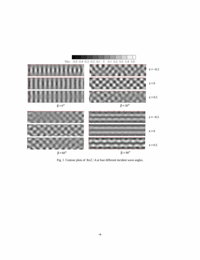
4. RESULTS As a numerical example, an isotropic plate with the stiffness varying in y-direction is studied. The bending and torsional rigidity is given by

��

���

� πε+===B

yDHDD xyyx2cos10 , �

�

���

� πε+ν=B

yDD 2cos101 . (9)

The dimensions and the structural properties of the runway are given by L = 5 km, B = 1 km, d = 5 m, h = 50 m, 0D =1.96 x 1011 N-m, ν = 0.3. In Fig 1., the deflections at four different incident wave angle, β, which is defined as the angle between x-axis and the wave angle, are compared for three different value of ε (see Eq. (9)): =ε -0.5, 0 and 0.5. The deflections are normalized by the amplitude of incoming wave, A. The incoming wavelength is 125 m or 20/ =λL . Total 150 by 30 panels are used to discretize the runway. In the head sea, the runway with the centerline stiffened (ε = 0.5) has a calmer runway surface. The runway with edges stiffened has undulations of greater height along the center of the runway, presumably because the transmitted waves are guided by the stiffened edges and not radiate to the water outside. On the other hand, in the oblique and beam seas, the runway with the stiffened edges is more calm. REFERENCES Bai, K. J., Yoo, B. S. and Kim, J. W. 2000 “A Localized Finite-Element Analysis of a Floating Runway in a Harbor,” (in print) Marine Structures. Ertekin, R.C. and Kim, J.W. 1999, “A Hydroelastic Response of a Floating, Mat-Type Structure in Oblique, Shallow-Water Waves,” Journal of Ship Research, Vol. 43, No.4 , pp. 241-254. Kashiwagi, M., 1998 “A B-Spline Galerkin Scheme for Calculating the Hydroelastic Response of a Very Large Floating Structure in Waves,” J. Marine Science and Technology, Vol. 3, pp37-49. Mamidipudi, P. and Webster, W. C. 1994 “The Motions Performance of a Mat-Like Floating Airport,” Hydroelasticity’94, Trondheim, Norway. Newman, J. N., Maniar, H. D. and Lee, C. H. 1996 “Analysis of Wave Effects for Very Large Floating Structures,” International Workshop on Very Large Floating Structures, Hayama, Japan, pp. 135-142. Webster, W. C. 1998 “Optimal Structure for Large-Scale Floating Runways,” Hydroelasticity in Marine Technology, Kashiwagi et al. (eds), RIAM, Kyushu University, pp. 15-26.

-4-

Fig. 1 Contour plots of A/Reζ at four different incident wave angles.

o0=β o30=β

o60=β o90=β

5.0−=ε

0=ε

5.0=ε

5.0−=ε

0=ε

5.0=ε