
Examensarbete Algorithmic Construction of Fundamental ...
91
Examensarbete Algorithmic Construction of Fundamental Polygons for Certain Fuchsian Groups David Larsson LiTH - MAT - EX - - 2015/05 - - SE
Transcript of Examensarbete Algorithmic Construction of Fundamental ...

Examensarbete
Algorithmic Construction of Fundamental Polygons forCertain Fuchsian Groups
David Larsson
LiTH - MAT - EX - - 2015/05 - - SE


Algorithmic Construction of Fundamental Polygons forCertain Fuchsian Groups
Mathematics and Applied Mathematics, Linkopings Universitet
David Larsson
LiTH - MAT - EX - - 2015/05 - - SE
Examensarbete: 30 hp
Level: A
Supervisor: Antonio F. Costa,Departamento de Matematicas Fundamentales,Universidad Nacional de Educacion a Distancia
Examiner: Milagros Izquierdo,Mathematics and Applied Mathematics,Linkopings Universitet
Linkoping: June 2015


Abstract
The work of mathematical giants, such as Lobachevsky, Gauss, Riemann,Klein and Poincare, to name a few, lies at the foundation of the study of thehighly structured Riemann surfaces, which allow definition of holomorphicmaps, corresponding to analytic maps in the theory of complex analysis.A topological result of Poincare states that every path-connected Riemannsurface can be realised by a construction of identifying congruent points inthe complex plane, the Riemann sphere or the hyperbolic plane; just threesimply connected surfaces that cover the underlying Riemann surface. Thisrequires the discontinuous action of a discrete subgroup of the automor-phisms of the corresponding space. In the hyperbolic plane, which is therichest source for Riemann surfaces, these groups are called Fuchsian, andthere are several ways to study the action of such groups geometrically bycomputing fundamental domains. What is accomplished in this thesis is acombination of the methods found by Reidemeister & Schreier, Singermanand Voight, and thus provides a unified way of finding Dirichlet domainsfor subgroups of cofinite groups with a given index. Several examples areconsidered in-depth.
Keywords: Compact Riemann surfaces and uniformization; Fuchsian groupsand automorphic functions; Hyperbolic geometry; Topological groups;Permutation groups; Computational methods; Covering spaces, branchedcoverings; Generators, relations, and presentations
URL for electronic version:
http://urn.kb.se/resolve?urn=urn:nbn:se:liu:diva-119916
Popularvetenskaplig sammanfattning
Nagra av de stora matematiker som har lagt grunden for de djupt struktur-erade Riemannytorna ar Lobachevsky, Gauss, Riemann, Klein och Poincare.Dessa ytor tillater oss att generalisera analytiska funktioner, kanda frankomplex analys, till holomorfa avbildningar. Ett av Poincares topologiskaresultat om dessa ytor ar att varje sammanhangande Riemannyta kan re-aliseras genom att identifiera punkter i en av tre ytor: det komplexa planet,
Larsson, 2015. v

vi
Riemannsfaren eller det hyperboliska planet. Alla tre ar dessutom enkeltsammanhangande och overtacker genom denna operation den underliggandeRiemannytan. Operationen innebar att en diskret undergrupp till ytans au-tomorfismgrupp tillats verka pa ytan. Det hyperboliska planet ger upphovtill de allra flesta Riemannytor och motsvarande grupper kallas i detta fallfor fuchsiska. For att studera dessa grupper och deras verkan geometrisktberaknas ofta fundamentalpolygoner. Var uppsats bidrar med en kombi-nation av metoder som upptackts av Reidemeister och Schreier, Singermanoch Voight, for att pa sa satt ge en enhetlig bild av hur Dirichletpolygonerkan beraknas for undergrupper, med ett givet index, till kofinita grupper.Flera exempel betraktas ingaende.
Acknowledgements
Standing on the shoulders of giants, I first of all want to posthumously thankall the pioneers of this fascinating subject.
Secondly, an enormous thanks to my supervisor, Antonio F. Costa, whoprovided much needed help throughout the process and averted several pos-sible embarassments. The same extends to my examiner, Milagros Izquierdo,who invested much time in setting up the thesis in cooperation with Anto-nio and also in helping me to understand David Singerman’s method andotherwise was of enormous help in spotting errors and perfecting the textas it now stands.
My opponent, Caroline Granfeldt, took a very serious approach to study-ing the thesis and without her opposition I could not have finished the workin time.
Furthermore, I want to thank my wife, Lydia, for her unending supportand for bearing with me during this thesis and even more during the processleading up to this climax. I want to thank my three wonderful children,Johannes, Maria and Teresa, for helping me to keep my eyes on the ultimatetrophy and not attach myself too much to earthly things.
I thank all my friends, who have provided much needed “whitespace” formy mind to work on. You know who you are!
Finally, but all the more important, I thank the heavenly court, mostespecially the Blessed Virgin Mary and Blessed Faa di Bruno, for theirintercession for me and the success of my mathematical studies.
Larsson, 2015. vii

viii

Symbols
Most of the reoccurring symbols that are not presumed to be known by thereader or have differing notation in the literature are described here.
A Surface atlases are in calligraphic style.Aut(X) The automorphism group of the space X.δA Boundary of the set A.
A Closure of the set A ⊂ X in X.
A Closure of the set A ⊂ X in X.z Complex conjugate of the complex number z.χ(G) Euler characteristic of a group G.[α, β] Geodesic between α and β.G,H, . . . Groups are denoted by capital letters starting with G.µ Hyperbolic area.ρ Hyperbolic norm and metric in U.ρ∗ Hyperbolic norm and metric in D.e Identity element in a group.[G : H] Index of H, as a subgroup of G.Ig Isometric circle associated to the Mobius transformation g.
A Interior of the set A.ker(θ) Kernel of the map θ.Ω Lattice in C.Γ The modular group.g, h, s, t Mobius transformations are denoted by small letters in this order.G · x Orbit of x under G.〈E|R〉 Presentation for some group.r Reduction map.Σ The Riemann sphere.pairs(F ) Side-pairing of a fundamental polygon F .sign(G) Signature of the Fuchsian group G.StabG(x) Stabiliser of x in G.U Upper half-plane model of the hyperbolic plane.D Unit disc model of the hyperbolic plane.
Larsson, 2015. ix

x

List of Figures
1.1 Fundamental domain for a lattice. . . . . . . . . . . . . . . . 1
2.1 Hausdorff separation. . . . . . . . . . . . . . . . . . . . . . . . 10
2.2 Surface atlas. . . . . . . . . . . . . . . . . . . . . . . . . . . . 11
2.3 Visualising cone points. . . . . . . . . . . . . . . . . . . . . . 13
2.4 Geodesics in the two models of the hyperbolic plane. . . . . . 15
2.5 Poincare models transformed. . . . . . . . . . . . . . . . . . . 16
2.6 Example of an isometric circle. . . . . . . . . . . . . . . . . . 18
3.1 Pasting the fundamental domain for a lattice. . . . . . . . . . 25
3.2 Fundamental domains for a lattice. . . . . . . . . . . . . . . . 26
3.3 Exchanging lattice domains. . . . . . . . . . . . . . . . . . . . 28
3.4 Action of an elliptic element. . . . . . . . . . . . . . . . . . . 31
3.5 Parabolic elements acting in hyperbolic 2-space. . . . . . . . . 31
3.6 Fundamental domain for triangle group with subgroup. . . . . 36
3.7 Examples of Reidemeister-Schreier graphs. . . . . . . . . . . . 37
4.1 Fundamental domains for finite Fuchsian groups. . . . . . . . 41
4.2 A Dirichlet domain for the modular group. . . . . . . . . . . 43
4.3 Example of a normalised boundary. . . . . . . . . . . . . . . . 48
5.1 Algorithmic computation for Γ. . . . . . . . . . . . . . . . . . 53
5.2 Implicit construction of fundamental domain for G2 . . . . . 54
5.3 Algorithmic computation for G2, all figures. . . . . . . . . . . 56
5.4 Algorithmic computation for G3,1, all figures. . . . . . . . . . 61
5.5 Algorithmic computation for G3,2, all figures. . . . . . . . . . 64
5.6 Algorithmic computation for Γ(2), all figures. . . . . . . . . . 66
Larsson, 2015. xi

List of Tables
3.1 Example of a Reidemeister-Schreier scheme. . . . . . . . . . . 37
5.1 Reidemeister-Schreier scheme for G2 ≤ Γ. . . . . . . . . . . . 545.2 G2: reductions and pairing. . . . . . . . . . . . . . . . . . . . 575.3 G2: Unpaired vertices in step 5. . . . . . . . . . . . . . . . . . 575.4 G2: Reductions on vertices in step 5. . . . . . . . . . . . . . . 585.5 G2: Reductions of elements in step 3, iteration 2. . . . . . . . 585.6 Reidemeister-Schreier scheme for G3,1 ≤ Γ. . . . . . . . . . . 595.7 G3,1: Reductions of elements in step 3, iteration 1. . . . . . . 595.8 G3,1: Unpaired vertices for iteration 1, step 5. . . . . . . . . . 605.9 G3,1: Reductions on vertices in step 5. . . . . . . . . . . . . . 605.10 Reidemeister-Schreier scheme for G3,2 ≤ Γ. . . . . . . . . . . 615.11 G3,2: Reductions of elements in step 3, iteration 1. . . . . . . 625.12 G3,2: Reductions on vertices in step 5, iteration 1. . . . . . . 625.13 G3,2: Reductions on vertices in step 5, iteration 2. . . . . . . 635.14 G3,2: Reductions on vertices in step 5, iteration 3. . . . . . . 635.15 Reidemeister-Schreier scheme for Γ(2) ≤ Γ. . . . . . . . . . . 65
List of algorithms
3.1 Finding the Dirichlet domain for a lattice Ω. . . . . . . . . . 273.2 The Reidemeister-Schreier algorithm. . . . . . . . . . . . . . . 384.1 Naively finding the Dirichlet domain for a Fuchsian group G. 404.2 Finding a normalised boundary for ext(H). . . . . . . . . . . 484.3 Computing redH(γ; z) = δ γ. . . . . . . . . . . . . . . . . . . 494.4 Computing a normalised basis for 〈H〉. . . . . . . . . . . . . . 50
xii Larsson, 2015.

Contents
1 Introduction 1
1.1 Historical Background . . . . . . . . . . . . . . . . . . . . . . 3
2 Basic Concepts 7
2.1 Group Theory . . . . . . . . . . . . . . . . . . . . . . . . . . . 7
2.2 Topology . . . . . . . . . . . . . . . . . . . . . . . . . . . . . 9
2.3 Covering Spaces . . . . . . . . . . . . . . . . . . . . . . . . . 12
2.4 Hyperbolic Geometry . . . . . . . . . . . . . . . . . . . . . . 14
2.5 Mobius Transformations . . . . . . . . . . . . . . . . . . . . . 17
3 Riemann Surfaces and Fuchsian Groups 21
3.1 Complex Curves are Real Surfaces . . . . . . . . . . . . . . . 21
3.2 The Euclidean Case . . . . . . . . . . . . . . . . . . . . . . . 23
3.3 Fuchsian Groups . . . . . . . . . . . . . . . . . . . . . . . . . 28
3.4 Fuchsian Subgroups . . . . . . . . . . . . . . . . . . . . . . . 33
4 Fundamental Domains for Fuchsian Groups 39
4.1 Dirichlet and Ford Domains . . . . . . . . . . . . . . . . . . . 39
4.2 Sides and Vertices on Fundamental Polygons . . . . . . . . . 45
4.3 Algorithmic Computation of Fundamental Domains . . . . . 46
5 Computations for Specific Fuchsian Groups 51
5.1 The Modular Group Γ . . . . . . . . . . . . . . . . . . . . . . 51
5.2 The Index Two Subgroup of Γ . . . . . . . . . . . . . . . . . 53
5.3 The First Index Three Subgroup of Γ . . . . . . . . . . . . . 58
5.4 The Second Index Three Subgroup of Γ . . . . . . . . . . . . 60
5.5 A Principal Congruence Subgroup of Γ . . . . . . . . . . . . . 65
6 Discussion 67
6.1 Suggestions for Further Study . . . . . . . . . . . . . . . . . . 68
A Code Transcripts 69
A.1 Common C++ Functions . . . . . . . . . . . . . . . . . . . . 69
A.2 Computing the Reduction Map in C++ . . . . . . . . . . . . 71
Larsson, 2015. xiii

xiv Contents
A.3 Displaying Vertex Pairings in C++ . . . . . . . . . . . . . . . 72A.4 Computing Right Cosets in GAP . . . . . . . . . . . . . . . . 73
Bibliography 75

Chapter 1
Introduction
Consider the vectors in the lattice displayed in Figure 1.1. The way integertranslations by these vectors act in the plane can be described by consideringa fundamental domain for the lattice, which is graphically represented asthe grey area. With this domain the correspondence between algebra andgeometry becomes clear, since the algebraic quotient C/Ω corresponds to thetopological construction of pasting the opposing sides of the quadrilateral.
Figure 1.1: Fundamental domain for a lattice.
However, this example covers only one of the cases which are interestingin the study of Riemann surfaces, i.e., surfaces with a complex structure thatmakes it possible to generalise analytic functions of one complex variable. Infact, only the torus arises in this way. The other special case is the sphere,and otherwise all compact surfaces are obtained by quotients, “pastings”, ofthe hyperbolic plane. Finding fundamental domains for the correspondinggroups, i.e., Fuchsian groups, is non-trivial, but in a lot of interesting cases
Larsson, 2015. 1
2 Chapter 1. Introduction
it is possible to employ an algorithm which ends in finite time, using onlythe generators of the group.
The three main objectives of this thesis is thus to: 1. explain the theoryof compact Riemann surfaces, Fuchsian groups and hyperbolic geometry;2. use a known structure of subgroups of Fuchsian groups to compute sig-natures and generators for certain subgroups of the modular group Γ; and3. show how to construct an algorithm to compute Dirichlet/Ford fundamen-tal domains, and apply it to the modular group and some of its subgroups.
More specifically, we make the following claims:
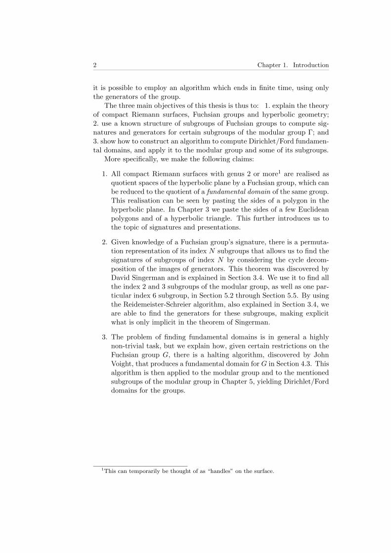
1. All compact Riemann surfaces with genus 2 or more1 are realised asquotient spaces of the hyperbolic plane by a Fuchsian group, which canbe reduced to the quotient of a fundamental domain of the same group.This realisation can be seen by pasting the sides of a polygon in thehyperbolic plane. In Chapter 3 we paste the sides of a few Euclideanpolygons and of a hyperbolic triangle. This further introduces us tothe topic of signatures and presentations.
2. Given knowledge of a Fuchsian group’s signature, there is a permuta-tion representation of its index N subgroups that allows us to find thesignatures of subgroups of index N by considering the cycle decom-position of the images of generators. This theorem was discovered byDavid Singerman and is explained in Section 3.4. We use it to find allthe index 2 and 3 subgroups of the modular group, as well as one par-ticular index 6 subgroup, in Section 5.2 through Section 5.5. By usingthe Reidemeister-Schreier algorithm, also explained in Section 3.4, weare able to find the generators for these subgroups, making explicitwhat is only implicit in the theorem of Singerman.
3. The problem of finding fundamental domains is in general a highlynon-trivial task, but we explain how, given certain restrictions on theFuchsian group G, there is a halting algorithm, discovered by JohnVoight, that produces a fundamental domain for G in Section 4.3. Thisalgorithm is then applied to the modular group and to the mentionedsubgroups of the modular group in Chapter 5, yielding Dirichlet/Forddomains for the groups.
1This can temporarily be thought of as “handles” on the surface.

1.1. Historical Background 3
1.1 Historical Background
There is no branch of mathematics, however abstract, whichmay not some day be applied to phenomena of the real world.—Nikolai Lobachevsky, [3, p. 572]
This thesis is placed in the intersection of three areas, which have hadparallel courses in history, but with considerable overlap. The intersection ofgeometry, both Euclidean and not, with complex function theory and grouptheory, has yielded and continues to yield much fruit. The connecting pointis Riemann surfaces.
We begin the story with the discovery of non-Euclidean geometry, sum-marised from [3, p. 585-590]. This was one of the most revolutionary discov-eries in geometry and was independently arrived at by three mathematicians:Nikolai Ivanovitch Lobachevsky (1793–1856), Carl Friedrich Gauss (1777–1855) and Janos Bolyai (1802–1860). The one who is credited with mostof the development of the theory is Lobachevsky, who published his workson what he called “imaginary geometry” in 1829. Even though Gauss hadbeen working on the same problem in about the same time as Lobachevskyand arrived at similar conclusions regarding the famous fifth, or parallel,postulate of Euclid (∼300 B.C.), he had not published any of his results andrefrained from doing so, even if he was quietly endorsing both Lobachevskyand Bolyai. The independent work of Bolyai was mainly obscured by hisown disappointment in not receiving priority in the discovery, which leadto him abandoning the pursuit altogether. Thus, the field was open forLobachevsky. The discovery he, and the other two, had made was that Eu-clid’s postulate that any line has a unique non-intersecting line through apoint not on that line could be replaced without losing logical consistency.The work was made concrete by instead using the postulate that any linehad infinitely many non-intersecting lines through a point not on the line.The astonishment that was felt by everyone, including the discoverers them-selves, can be garnered from the term that Lobachevsky had used for thistype of geometry.
Another leap forward was made by Georg Friedrich Bernhard Riemann(1826–1866) in two steps. First he published his doctoral thesis on complexfunctions of one variable, introducing Riemann surfaces as a way of visu-alising the multiple-valued functions appearing in complex analysis, suchas the complex logarithm. Later, as a step in his academic career, he wasrequired to hold a lecture, his Habilitation, which introduced the notions ofhigher-dimensional equivalents of surfaces, which he called manifolds, andalso generalised differential geometry by noticing that the metric associ-ated to Euclidean geometry was only one of many metrics. He went evenfurther and connected the Gaussian curvature of a surface to the metric.This connection gives one way of distinguishing three, in one sense “basic”,

4 Chapter 1. Introduction
geometries:
• the Euclidean plane, with constant Gaussian curvature 0;
• the sphere, with constant Gaussian curvature 1;
• the hyperbolic plane, with constant Gaussian curvature −1.
The work was further generalised by Adolf Hurwitz (1859–1919), who firstconsidered Riemann surfaces as branched covering surfaces of the Riemannsphere, in [10].
Building on the work of Riemann, Eugenio Beltrami (1835–1900) wasthe first to give a model for Lobachevskian, or hyperbolic, geometry withthe pseudo-sphere, giving a way to visualise hyperbolic geometry, whichhad up until this time been researched in axiomatic terms. Furthermore,he thus gave hyperbolic geometry an equal footing with Euclidean geome-try and by the pseudo-sphere it inherited its geometry from its Euclideancousin. This was to be followed by models by Felix Klein (1849–1925) andHenri Poincare (1854–1912), [3, p. 580, 591–594, 650–654]. The former isperhaps most famous for his Erlanger Programm, wherein he showed how touse group theory in conjunction with geometry and thereby distinguishinggeometries by certain invariants under group action. One part of this wasshowing how Euclidean geometry was a special case of affine geometry, whichin turn was a special case of projective geometry. Klein showed this via lin-ear fractional transformations, also known as Mobius transformations, afterthe mathematician August Ferdinand Mobius (1790–1860) who had studiedthem extensively earlier. The latter of the two, Poincare, had done his doc-toral thesis on existence theorems for differential equations, which includedproperties of automorphic functions, which are meromorphic2 complex func-tions invariant under a countable group of Mobius transformations. He wasthe one who insisted on the name Fuchsian groups, since they characterisethe functions he considered in this dissertation, which were Fuchsian func-tions, while Klein wanted to name them Schwartzian. Poincare was regardedas a universal mathematician, taking on a wide variety of areas. Among themore noteworthy in regards to our thesis is his work in establishing muchof the foundations for algebraic topology. Even though work had been donein this area earlier, it is widely recognised that Poincare’s work on analysissitus, as it was called, was a starting point for the much wider and deeperinterest that emerged during the 20th century.
Another character that we encounter in this story [3, p. 662, 668] isHermann Weyl (1885–1955), who also worked in this field and in a 1913lecture on Riemann surfaces had emphasised the abstract nature of the 2-manifolds which bore the name of Riemann surfaces.
2Analytic except for poles.

1.1. Historical Background 5
A revival of interest in the area at hand was to come in the 1960s, whenAlexander Murray MacBeath (1923–2014) and his students started usingcombinatorial methods to study Fuchsian groups and Riemann surfaces.Notable among them is David Singerman which has influenced this thesisimmensely, by inheritance.
The work done in this area is vast and there are many other charactersthat could be mentioned. Thus, the above is a brief overview of the centuries-old roots of the current thesis.

6 Chapter 1. Introduction

Chapter 2
Basic Concepts
Given the nature of a master thesis, we aim to be as self-contained as pos-sible, thus reiterating concepts that may already have been encountered.Moreover, it is useful to fix notation even for basic concepts. Thus, we willwalk through some of the prerequisites for understanding this thesis.
2.1 Group Theory
The first concept we need to deal with is that of a group. Even though thisconcept took time to develop, its mature form is fairly straight-forward inits basic concepts. Employing these basic notions has proven to be a veryfruitful and challenging area of ongoing research.
Recall that a group (G, ·) is a set G accompanied by the operation ·,that satisfies the following properties, see [9, p. 13],
(i) Associativity: x · (y · z) = (x · y) · z for all choices of x, y, z ∈ G;
(ii) Existence of an identity: There is a unique element e ∈ G such thate · g = g · e = g for all g ∈ G;
(iii) Existence of inverse: For every x ∈ G, there is an inverse x−1 ∈ Gsuch that x · x−1 = x−1 · x = e.
Remark 2.1. We will almost everywhere1 abbreviate x · y as xy. In thecase of a commutative group operation · is often denoted by +. The identityin this case will be denoted 0.
Permutation groups hold a special place in our thesis, so we define apermutation as a bijective function on a finite set of symbols X, see [9,p. 107-110]. In this thesis we will always take the symbol set as contiguous
1The set of places where we write out · is even finite!
Larsson, 2015. 7

8 Chapter 2. Basic Concepts
positive integers starting at 1, so X = 1, 2, . . . , n. This bijection can berepresented in several ways. First, by explicitly giving the bijection, as(
1 2 3 4 52 3 1 4 5
),
which means that 1 maps to 2, which maps to 3, which maps back to 1,while 4 and 5 remain fixed.
This illustrates that there is a more convenient way to represent thispermutation. The canonical decomposition of the permutation into disjointcycles is then written as
(1, 2, 3)(4)(5),
where we get both the orbit of each element under the permutation as wellas the order of the mapping of elements.
Multiplication of permutations is then most easily described by an ex-ample, from which the reader can infer the general pattern, recalling thatthe first permutation to be applied is the one on the right,
(1, 2)(1, 3, 2) = (1, 3)(2),
(1, 3, 2)(1, 2) = (1)(2, 3).
The first line shows that 1 maps to 3 by the first permutation and then 3 isnot altered by the second. Then, 3 maps to 2 by the first which is mappedto 1 by the second and 2 remains fixed after applying both permutations.
Needing to make transitions between groups, we introduce certain mapsbetween groups, see [9, p. 98-99, 102]. First, let G, H be groups. A grouphomomorphism θ : G→ H is such that for every g, h ∈ G,
θ(g−1) = θ(g)−1 and θ(gh) = θ(g)θ(h).
A group isomorphism is a bijective homomorphism and an epimorphism isa surjective homomorphism. Moreover, a group automorphism is an isomor-phism of a group with itself, which need not be the identity. The kernel ofa homomorphism is the pre-image of the unit element
ker(θ) = θ−1(e).
Moreover, some subsets and subgroups of G are particularly interesting,see [8, p. 55]. Let G be a group acting on X. Then, the stabiliser of a pointx ∈ X is the subgroup
StabG(x) = g ∈ G : g(x) = x.
Moreover, the orbit of a point x ∈ X under G is the set
G · x = y ∈ X : ∃g ∈ G : g(x) = y,

2.2. Topology 9
i.e., all the points reached from x by elements in G. As an example, thegroup generated by (1, 2, 3)(4)(5) consists of only three elements, all fixing4 and 5. Thus, the orbit of 4 and 5 under this group is simply 4 and 5,while for 1, 2 and 3 their common orbit will be 1, 2, 3.
Let H ≤ G be groups. A conjugation, [9, p. 126], of h ∈ H by g ∈ G isthe element
ghg−1 ∈ G,
with its conjugacy class being the equivalence class of all possible conjuga-tions of h by g in G.
A conjugation of the subgroup H by g is the subgroup
gHg−1 = s ∈ G : s = ghg−1, h ∈ H ≤ G.
Finally, if a subgroup H ≤ G has n left cosets in G, which means thatH splits G into n equivalence classes, it is said to be of index [G : H] = n,see [8, p. 16].
2.2 Topology
A brief recapitulation of topological notions is also warranted, and the def-initions in this section are taken from Jones & Singerman [13, p. 167-172]and Munkres [15, p. 76, 98, 137-139].
The main tools in the topological toolbox we will use are covering spaces.In order for this to make sense, we start at the beginning.
Definition 2.1. Let X be a set and τ ⊂ P(X). The ordered pair (X, τ),often abbreviated X, is a topological space if
(i) ∅, X ∈ τ .
(ii) Let Λ be an arbitrary index set. If, for every λ ∈ Λ, Aλ ∈ τ , then theunion
⋃λ∈ΛAλ ∈ τ .
(iii) If A,B ∈ τ , then A ∩B ∈ τ .
The sets in τ are called open and their complements are called closed.
Remark 2.2. Let X be a universal set. We fix the following notation: D isthe interior of D, i.e., the maximal open subset of D. Further, Dc = X \Dis the complement of D. In the following, we will also use D for the closure
of D in X, i.e., the minimal closed superset of D and D for the closure ofD in X. Finally, we denote the boundary by δD = D \ D.
A space in and of itself is not so interesting, unless we have operationsthat we can use on them. The main tool in comparing topological spaces

10 Chapter 2. Basic Concepts
is homeomorphism2, which is an open, continuous bijection between twospaces. Imagine that you can move between the spaces in the sense that youcan continuously deform one into the other. To be more precise, a mappingp is open if it maps open sets to open sets, and continuous if every point inthe image of p has an open neighbourhood such that its pre-image is openin the domain of p. Furthermore, p : X → Y is a bijection if every pointin the domain gets mapped to at most one point in Y and every point inY has a non-empty pre-image. This extends also to subsets of X and Y , inthe following definition.
Definition 2.2. Let X,Y be topological spaces. Two open sets U ⊂ X andV ⊂ Y are homeomorphic if there is a homeomorphism between U and V .
In terms of our thesis, the most interesting form of topology is that ofa surface. Using these topological terms, the extension of the definition tohigher dimensional equivalents of surfaces, called n-manifolds, is nowadayseasy3. The theory surrounding higher-dimensional geometry is far from easy,however.
Definition 2.3. A surface, or 2-manifold, is a Hausdorff topological spaceS, such that for every point s ∈ S, there is an open set U 3 s that ishomeomorphic to an open subset V ⊂ R2.
The importance of the constraint that S is a Hausdorff space might bemore apparent if this is understood to mean that our notion of what canbe said of distinct points in Euclidean space is also true of surfaces. Thisrestriction means that we require the topology of S be such that any two,distinct, points s1, s2 can be separated by open sets, i.e., there are openneighbourhoods S1 3 s1 and S2 3 s2 such that S1 ∩S2 = ∅. See Figure 2.1.
Figure 2.1: Two distinct pointscan be separated by open sets inHausdorff spaces.
In order to find ourselves around a sur-face, we need some sense of where we are.The analogous terms that are employed inthe definitions of coordinate systems on sur-faces should be kept in mind.
Definition 2.4. Let S be a surface. Achart for, not necessarily all of, S is an or-dered pair (U, φ), such that φ is a homeo-morphism between U ⊂ S and φ(U) ⊂ R2.An atlas for S is a set of charts, A, such that S =
⋃(U,φ)∈A U and moreover,
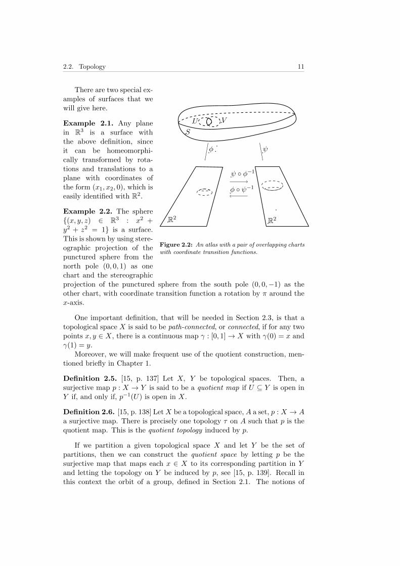
if S ⊃ U ∩ V 6= ∅, with charts (U, φ) and (V, ψ), we define the coordinatetransition functions as φ ψ−1 : ψ(U ∩ V ) → φ(U ∩ V ) (and its inverse).The definition is illustrated in Figure 2.2.
2Not to be confused with homomorphism.3The historical development of this notion shows that this was not always the case.
2.2. Topology 11
R2 R2
S
U V
φ ψ
ψ φ−1
φ ψ−1
Figure 2.2: An atlas with a pair of overlapping chartswith coordinate transition functions.
There are two special ex-amples of surfaces that wewill give here.
Example 2.1. Any planein R3 is a surface withthe above definition, sinceit can be homeomorphi-cally transformed by rota-tions and translations to aplane with coordinates ofthe form (x1, x2, 0), which iseasily identified with R2.
Example 2.2. The sphere(x, y, z) ∈ R3 : x2 +y2 + z2 = 1 is a surface.This is shown by using stere-ographic projection of thepunctured sphere from thenorth pole (0, 0, 1) as onechart and the stereographicprojection of the punctured sphere from the south pole (0, 0,−1) as theother chart, with coordinate transition function a rotation by π around thex-axis.
One important definition, that will be needed in Section 2.3, is that atopological space X is said to be path-connected, or connected, if for any twopoints x, y ∈ X, there is a continuous map γ : [0, 1]→ X with γ(0) = x andγ(1) = y.
Moreover, we will make frequent use of the quotient construction, men-tioned briefly in Chapter 1.
Definition 2.5. [15, p. 137] Let X, Y be topological spaces. Then, asurjective map p : X → Y is said to be a quotient map if U ⊆ Y is open inY if, and only if, p−1(U) is open in X.
Definition 2.6. [15, p. 138] LetX be a topological space, A a set, p : X → Aa surjective map. There is precisely one topology τ on A such that p is thequotient map. This is the quotient topology induced by p.
If we partition a given topological space X and let Y be the set ofpartitions, then we can construct the quotient space by letting p be thesurjective map that maps each x ∈ X to its corresponding partition in Yand letting the topology on Y be induced by p, see [15, p. 139]. Recall inthis context the orbit of a group, defined in Section 2.1. The notions of

12 Chapter 2. Basic Concepts
discreteness, that we will introduce later, allow us to create such a quotientspace by mapping each point of a given space onto its orbit under a givengroup. Later, this will be made more concrete in terms of the discrete groupswe consider in this thesis.
Finally, the genus of a surface is defined as the maximal number of curveson the surface that, when we cut the surface along these curves, does notdisconnect the surface (see [13, p. 163]). We can equivalently think of it asthe number of “handles” in the surface. To see this, consider Figure 3.1 andconvince yourself that the maximal number of closed curves that does notdisconnect the torus is 1. The genus for a group is moreover defined as thegenus of the quotient surface arising from the group. The latter definitioncould be given purely algebraically in terms of the structure of generators,which will be touched upon in Section 3.3, together with other phenomenalike cusps and cone points.
2.3 Covering Spaces
Of interest in our thesis is also a topological notion that relates the funda-mental domains of subgroups to the fundamental domain of the larger group:covering maps and covering spaces. We start with an abstract definition.
Definition 2.7. [14, p. 145] Let X be a path-connected, topological space.An n-sheeted covering space (abbreviated as n-sheeted covering), with 1 ≤n ≤ +∞, for X is a pair (X, p), where X is a topological space and p :X → X satisfies the following condition: for every point x ∈ X, there is anopen neighbourhood U 3 x such that p−1(U) is a disjoint union of n opensets that is each homeomorphically mapped onto U . The map p is called ann-sheeted covering map or a projection.
As obvious examples, Massey [14, p. 146] gives us that all homeomor-phisms φ : X → X are 1-sheeted coverings of X. Many, more interesting,examples exist. For instance, quotient surfaces without cone points, dis-cussed later, are covered by the original surface.
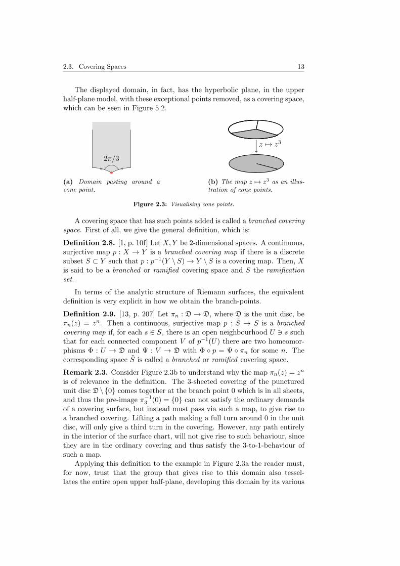
There is a problem with restricting ourselves to the covering spaces de-scribed, however, since it is often the case in dealing with quotient surfaces,and eminently so in our thesis, that there are exceptional points that giverise to fewer than n sheets in the pre-image, called branch-points or conepoints, [13, p. 207]. Intuitively, this means that when turning a full rotationaround the point, only part of a full rotation is actually accomplished. Itis probably easier to understand with a picture, see Figure 2.3a. The anglebetween the two sides at the red point is 2π/3. Thus, when identifying thetwo sides marked by arrows, making a turn around the red point will onlyresult in a third of a turn.
2.3. Covering Spaces 13
The displayed domain, in fact, has the hyperbolic plane, in the upperhalf-plane model, with these exceptional points removed, as a covering space,which can be seen in Figure 5.2.
2π/3
(a) Domain pasting around acone point.
z 7→ z3
(b) The map z 7→ z3 as an illus-tration of cone points.
Figure 2.3: Visualising cone points.
A covering space that has such points added is called a branched coveringspace. First of all, we give the general definition, which is:
Definition 2.8. [1, p. 10f] Let X,Y be 2-dimensional spaces. A continuous,surjective map p : X → Y is a branched covering map if there is a discretesubset S ⊂ Y such that p : p−1(Y \ S)→ Y \ S is a covering map. Then, Xis said to be a branched or ramified covering space and S the ramificationset.
In terms of the analytic structure of Riemann surfaces, the equivalentdefinition is very explicit in how we obtain the branch-points.
Definition 2.9. [13, p. 207] Let πn : D → D, where D is the unit disc, beπn(z) = zn. Then a continuous, surjective map p : S → S is a branchedcovering map if, for each s ∈ S, there is an open neighbourhood U 3 s suchthat for each connected component V of p−1(U) there are two homeomor-phisms Φ : U → D and Ψ : V → D with Φ p = Ψ πn for some n. Thecorresponding space S is called a branched or ramified covering space.
Remark 2.3. Consider Figure 2.3b to understand why the map πn(z) = zn
is of relevance in the definition. The 3-sheeted covering of the puncturedunit disc D\0 comes together at the branch point 0 which is in all sheets,and thus the pre-image π−1
3 (0) = 0 can not satisfy the ordinary demandsof a covering surface, but instead must pass via such a map, to give rise toa branched covering. Lifting a path making a full turn around 0 in the unitdisc, will only give a third turn in the covering. However, any path entirelyin the interior of the surface chart, will not give rise to such behaviour, sincethey are in the ordinary covering and thus satisfy the 3-to-1-behaviour ofsuch a map.
Applying this definition to the example in Figure 2.3a the reader must,for now, trust that the group that gives rise to this domain also tessel-lates the entire open upper half-plane, developing this domain by its various

14 Chapter 2. Basic Concepts
transformations. Thus, we can consider the open upper half-plane as aninfinite-sheeted ramified covering space for the domain.
Subgroups will also give rise to covering spaces, as will be seen, whenconsidering an index 6 subgroup of a Fuchsian triangle group in Section 3.4,which gives rise to a 6-sheeted branched covering of the initial group’s fun-damental domain.
As a preemption of the deep uniformisation theorem, Theorem 3.3, wedefine a universal covering space U of X as a covering space of X thatis, moreover, simply connected, which means that any path in U can becontinuously transformed to a point.
2.4 Hyperbolic Geometry
In order to move to the more mind-bending world of Fuchsian groups, wemust first introduce hyperbolic space. The perspective of projective geome-try gives us a way to characterise parallel Euclidean lines as those lines thatmeet at a point at infinity. Thus, the uniqueness of parallel lines correspondsto the “uniqueness of infinity”. However, in hyperbolic geometry, there isno such uniqueness. Indeed, given a hyperbolic line l and a point p in thehyperbolic plane not on l, there are infinitely many distinct lines `i goingthrough p that do not intersect l. And, correspondingly, there is an entire“circle at infinity”. In order to distinguish the two different cases, however,not all of them are normally called parallel lines. If `i meets l in a pointon the circle at infinity it is defined as parallel and otherwise it is calledultraparallel. We mainly follow Beardon [2, p. 126-187], except for his useof the terminology parallel and disjoint in this case.
We will use two models that satisfy the above property, Poincare’s unitdisc and upper half-plane models. Several other ways of realising the hyper-bolic plane exist, with properties that can be useful in other contexts, butour choice is both a matter of custom and a consequence of the theoremsand techniques we are interested in, which are driven towards these models.
Definition 2.10. [2, p. 126f] The upper half-plane model of the hyperbolicplane is the set U = z : Im(z) > 0 together with the hyperbolic metric ρ,defined by the differential
ds =|dz|Im z
.
The open unit disc model of the hyperbolic plane is the set D = z :|z| < 1 together with the hyperbolic metric ρ∗, defined by the differential
ds =2 |dz|
1− |z|2.
The circle at infinity is defined as δD = z : |z| = 1 for the disc modeland δU = R ∪ ∞ for the upper half-plane model.

2.4. Hyperbolic Geometry 15
Figure 2.4: Geodesics in the two models of the hyperbolic plane.
To calculate the length of a curve in the hyperbolic plane is then amatter of path integration over a parametrisation of the curve with thegiven differential substituting the Euclidean differential |dz|. Let γ(I) ⊂ Uor δ(I) ⊂ D be a path of the hyperbolic plane, with the standard notationz = x+ iy. Then,
ρ(γ) =
∫γ
|dz|Im z
=
∫ 1
0
√(dx/dt)2 + (dy/dt)2
ydt,
ρ∗(δ) =
∫δ
2 |dz|1− |z|2
∫ 1
0
2√
(dx/dt)2 + (dy/dt)2
1− (x2 + y2)dt
In order to find the shortest path between two given hyperbolic points z, w,we simply minimise the integral over all the paths between z and w. Thispath is part of a geodesic, which is the equivalent to a Euclidean straightline.4 The general form of the geodesics has been derived, so that we neednot perform the process of minimising ρ(γ) in an ad hoc fashion. In the“normal” case, the geodesics are Euclidean circles orthogonal to the circle atinfinity, in either model. However, in the upper half-plane, when the pointshave the same real part, we instead get a geodesic that is a vertical Euclideanstraight half-line, and in the disc, when the unique Euclidean line throughthe points contains the origin, the Euclidean line segment inside the unitdisc is the hyperbolic geodesic containing the points, explained by Beardonin [2, p. 129-136], see Figure 2.4. Thus, the geodesics are the generalisedEuclidean circles orthogonal to the circle at infinity and we will denote thegeodesic between α and β as [α, β]. This characterisation further makes itpossible to find the hyperbolic distance efficiently, as in Theorem 2.11.
Theorem 2.11. Let z, w ∈ U. The hyperbolic distance ρ(z, w) can becomputed by either of the following formulas, used in Appendix A.1:
(i) If z = iy, w = iv, with v > y then ρ(z, w) = ln(v/y).
(ii) ρ(z, w) = ln (|z − w|+ |z − w|) / (|z − w| − |z − w|).
4For a more physical intuition, consider the geodesics as least energy paths.

16 Chapter 2. Basic Concepts
Defining the hyperbolic area follows a similar vein as the definition ofhyperbolic length. For a set E ⊂ U, we define the hyperbolic area as thedouble integral
µ(E) =
∫∫E
dx dy
y2.
In this case, the non-trivial Gauss-Bonnet theorem gives us a way to computethe area of a given polygon with known angles.
Theorem 2.12. [13, Theorem 5.5.2., p. 229] (Gauss-Bonnet) For a hyper-bolic triangle ∆ with angles α, β, γ ≥ 0, µ(∆) = π − α− β − γ.
Corollary 2.13. [13, Corollary 5.5.6., p. 230] For a hyperbolic n-gon P ,that is hyperbolically convex, with angles v1, v2, . . . , vn,
µ(P ) = (n− 2)π −n∑k=1
vk
Remark 2.4. A set is hyperbolically convex if the geodesic line segmentbetween any two points is entirely inside the set, directly translated fromEuclidean geometry.
p
Figure 2.5: The homeomorphism p betweenthe Poincare upper half-plane and disc mod-els of hyperbolic geometry.
Moving between the two modelsis achieved by applying the follow-ing homeomorphism between thetwo models that moreover preservesthe hyperbolic structure, i.e., it is anisometry between U with the met-ric ρ and D with the metric ρ∗, asstated in [2, p. 131] and [20, p. 470].
Example 2.3. The transformation,
p(z) =z − kz − k
,
with Im k > 0, maps the upper half-plane z : Im z > 0 to the open unitdisc z : |z| < 1 bijectively. Thus, its inverse exists and is
p−1(z) =kz − kz − 1
.
Since both p and p−1 are continuous and defined on the entirety of theirrespective domain, p is a homeomorphism. The transformation, in the casek = i, is illustrated in Figure 2.5 with the mapping of one interior pointand two boundary points (i 7→ 0, 0 7→ −1, 1 7→ −i). The transformations,moreover, are conformal, i.e., preserves angles, since they are holomorphicmaps between the two spaces, see Section 3.1.

2.5. Mobius Transformations 17
2.5 Mobius Transformations
The final example in Section 2.4 was a particular example of the fundamen-tal building blocks of Fuchsian groups, which are linear fractional transfor-mations. The wealth of material describing and illuminating these Mobiustransformations means that we can only give a brief introduction, focusedon the scope of our thesis.
Definition 2.14. [13, p. 17] A Mobius transformation g is a function of theform
g(z) =az + b
cz + d, ad− bc 6= 0, a, b, c, d ∈ C.
Remark 2.5. This concept can be generalised to higher dimensions byPoincare’s extension method, described extensively in Beardon [2, Ch. 3.3].
The observant reader notices an immediate similarity between this repre-sentation of a linear fractional transformation and the matrix group GL(2,C).Recall that this group is the family of square matrices,(
a bc d
), ad− bc 6= 0, a, b, c, d ∈ C,
defined in [13, p. 18]. One could be tempted to try to define a group isomor-phism between these two concepts. However, notice that the Mobius trans-formation remains invariant when multiplying all elements by some non-zeroscalar. This is obviously not true in GL(2,C), but can be remedied if weconstruct the quotient group GL(2,C)/λI : λ 6= 0, where we identify allthe matrices which differ only by a scalar multiple. Then an isomorphismis accomplished by simply identifying the coefficients in the two groups andthis abstract group is called the projective general linear group PGL(2,C)over the field C. When the field is C, we have a special situation, becausethen PGL(2,C) is equal to the projective special linear group PSL(2,C),which is instead defined as the special linear group of square matrices,(
a bc d
), ad− bc = 1, a, b, c, d ∈ C,
quoted by the set I,−I. This is not true when we want to move to groupsover the field R, which Example 2.4 demonstrates.
Example 2.4. Consider the Mobius transformation g(z) = (3z+4)/(z+2),which can be represented in GL(2,R) as(
3 41 2
)

18 Chapter 2. Basic Concepts
with entries corresponding to the coefficients of g. However,
3z + 4
z + 2=
3λz + 4λ
λz + 2λ
for any λ 6= 0 and thus has infinitely many representatives in GL(2,R).As can easily be seen, no multiplication with a real λ 6= 0 will ever yielda negative determinant in the matrix representative, since λ2 ≥ 0, whichimplies that the topological group PGL(2,R) is disconnected, with PSL(2,R)inside the connected component with pre-images in GL(2,R) of positivedeterminant. Since the matrix representatives in GL(2,R) with determinantprecisely 1 are unique, we can identify the Mobius transformations with realcoefficients with elements in PSL(2,R).
Remark 2.6. Since the identification of Mobius transformations with theirmatrix representatives is so common, we will slightly abuse notation, byletting g, h, s, t, . . . refer to both the functional representation of an elementand the matrix representative of the same element.
As the preceding example states, the group PSL(2,R) is topological, afact that is explored in more detail in Section 3.3. With the field of complexnumbers, we could move more easily between the general linear form andthe special linear form, but as a consequence of the above, we need to bemore careful when working with the real numbers. However, we can choosematrix representatives in PGL(2,R) as long as we stay in the connectedcomponent of PSL(2,R), i.e., we enforce the restriction ad− bc > 0. Thus,we define a real Mobius transformation as a transformation
g(z) =az + b
cz + d, a, b, c, d ∈ R, ad− bc > 0.
Ig
Figure 2.6: Example of an isomet-ric circle.
When moving to Fuchsian groups in Sec-tion 3.3, we will use a sequential definitionof discreteness, following Beardon [2, p. 11-15] so that a subgroup G ≤ PSL(2,R) isdiscrete if any sequence Ak∞k=1 ⊆ G suchthat ak, dk → 1, bk, ck → 0 as k → ∞ im-plies that Ak = I for all but finitely manyk. There are other equivalent definitions ofdiscreteness, but, in view of the groups wewill discuss, this seems the most appropri-ate.
A natural question is why PSL(2,R) isthe natural group to consider in hyperbolicspace. This is because this group is one of the crucial descriptors of hyper-bolic geometry. Indeed, PSL(2,R) is the automorphism group of the upper

2.5. Mobius Transformations 19
half-plane model of hyperbolic space, where the automorphism group, de-noted by Aut(X), is defined as the group of all conformal homeomorphismsof a given space X. That PSL(2,R) ⊂ Aut(U) is a direct result of the follow-ing theorem. The other inclusion can be deduced via the theory of analyticfunctions, see [13, Theorem 4.17.3].
Theorem 2.15. [13, Theorem 5.3.1] For every g ∈ PSL(2,R) and everypath γ(I) ⊂ U,
ρ(g(γ)) = ρ(γ).
An immediate consequence is, by [13, Theorem 5.3.5], for every pair z, w ∈ U,
ρ(g(z), g(w)) = ρ(z, w).
Finally, one of the important geometric descriptors of a Mobius trans-formation is the isometric circle, and for g(z) = (az+ b)/(cz+d) with c 6= 0and ad − bc = 1, is defined as the set Ig = z : |cz + d| = 1. In the casec = 0, there is no unique circle with the same properties, and then we define,in view of Section 4.3, Ig = C. Moreover, we define the isometric line ofg as the (Euclidean) perpendicular bisector of the line between the centresof Ig and Ig−1 . An example of an isometric circle in hyperbolic geometry isgiven in Figure 2.6.
This definition will be amply used in Section 4.1, Section 4.3 and through-out Chapter 5, where the fact that these isometric circles are also hyperbolicgeodesics is utilised. However, before going there, we need to delve deeperinto the theory of Riemann surfaces and Fuchsian groups.

20 Chapter 2. Basic Concepts

Chapter 3
Riemann Surfaces andFuchsian Groups
... I left Caen, where I was living, to go on a geologic excur-sion under the auspices of the School of Mines. The incidentsof the travel made me forget my mathematical work. Havingreached Coutances, we entered an omnibus to go to some placeor other. At the moment when I put my foot on the step, theidea came to me, without anything in my former thoughts seem-ing to have paved the way for it, that the transformations I hadused to define the Fuchsian functions were identical with those ofnon-Euclidean geometry. I did not verify the idea; I should nothave had time, as upon taking my seat in the omnibus, I wenton with a conversation already commenced, but I felt a perfectcertainty. On my return to Caen, for convenience sake, I verifiedthe result at my leisure. —Henri Poincare, [16, p. 387f]
3.1 Complex Curves are Real Surfaces
We begin by specifying the characteristics of Riemann surfaces in terms oftopology, i.e., building on Section 2.2. The definitions in this section aretaken from Jones & Singerman [13, p. 167-172], and we make the naturalidentification of C with R2. We start with an example to tie us back to theprevious work.
Example 3.1. [13, p. 2f, 169] In the context of compact Riemann surfaces,one of two special cases is the Riemann sphere. We begin by showing thatthe Riemann sphere is indeed a surface. First of all, the Riemann sphere isdefined as
Σ = C ∪ ∞,
Larsson, 2015. 21

22 Chapter 3. Riemann Surfaces and Fuchsian Groups
where ∞ is a single point added, such that z → ∞ whenever |z| → +∞(distinguishing the point ∞ from the potential infinity +∞). It is thennatural to define
1
0=∞, 1
∞= 0.
An atlas A for Σ consists of two charts, (C, z) and (Σ \ 0, 1/z). Thus, Σis a surface. To show that Σ is a Riemann surface we only need to showthat these two charts are analytically compatible. The coordinate transitionfunctions become z 7→ 1/z on C \ 0 in both directions. Clearly this mapis analytic on C \ 0 and corresponds to rotation around the x-axis inExample 2.2. This means that the charts are indeed analytically compatible.
The abstract definition of a Riemann surface requires us to restrict at-tention to a certain class of surfaces with a particular structure. It boilsdown to requiring that we can define analogues of the analytic maps fromC into C, called holomorphic maps. Hence, an analytic atlas is an atlaswith analytic coordinate transition functions. Thus, since the coordinatetransition functions in Example 3.1 are both analytic, the Riemann sphereis a Riemann surface. Two analytic atlases are (analytically) compatible ifA∪B is an analytic atlas. Similarly, one can define other atlases, with othernotions of compatibility1. Now, compatibility is an equivalence relation, soif there are different equivalence classes of compatible analytic atlases for agiven surface, then they will give rise to different structures on the surface,which motivates the definition of a complex structure as an equivalence classof analytic atlases. Equivalently, one could define the complex structure asthe maximal atlas with respect to analyticity.
All the preceding makes it possible to state what a Riemann surface isin a sentence.
Definition 3.1. A Riemann surface is a surface S with a complex structure.
A map f : S1 → S2 between two Riemann surfaces S1 and S2 is thensaid to be holomorphic if it satisfies the condition that for any pair of charts(U1, φ1) and (U2, φ2), respectively for the two surfaces, where f−1(U2)∩U1 6=∅, the induced function φ2 f φ−1
1 : φ1(f−1(U2) ∩ U1)→ C is analytic.
The natural equivalence between Riemann surfaces, corresponding tosuch notions as homeomorphic in a topological sense, is that of conformalequivalence, which means that there is a holomorphic homeomorphism be-tween the two surfaces, i.e., preserving both the topological and complexstructures on the surface. The conformality of the equivalence is due to thefollowing proposition.
1For instance, the compatibility of geometric structures, arising from different metricson the surface.

3.2. The Euclidean Case 23
Proposition 3.2. [13, p. 198] Let f : S1 → S2 be a holomorphic homeo-morphism. Then, f−1 : S2 → S1 is a holomorphic homeomorphism and fand f−1 are conformal maps.
Remark 3.1. By using local coordinates, the proof reduces to showing thatanalytic homeomorphisms are conformal between two open sets U, V ⊆ C.
This moves us to a remarkably deep result of Poincare, Klein and Koebe:all connected Riemann surfaces have one of three universal covering spaces.This is called the uniformisation theorem.
Theorem 3.3. [13, Theorem 4.17.2, p. 200] Every simply connected Rie-mann surface is conformally equivalent to precisely one of:
(i) the Riemann sphere Σ,
(ii) the complex plane C, or
(iii) the hyperbolic plane (in the disc model D or the upper half-planemodel U).
Thus, the surfaces are all obtained by making the quotient of the univer-sal covering space with a discrete subgroup of the automorphism group ofthe universal covering space, see [13, p. 213f], the corresponding groups areso-called fundamental groups for the arising surface. As seen in Example 3.1,the Riemann sphere is of genus 0. In fact, it is the only compact Riemannsurface of genus 0 and the only one arising from spherical geometry. Thefocus of our thesis is on the third possibility, but first we make a detour toquotients of the complex plane.
3.2 The Euclidean Case
The single Riemann surface which arises from Euclidean geometry is thetorus, which we now introduce. The material is a synthesis of Beardon [2],Coxeter & Moser [4], Jones & Singerman [13], Voight [20] and Zieschang &al.[22]. The torus arises in a way that is a very good introduction to the waythe rest of the compact Riemann surfaces arise in the setting of hyperbolicgeometry. First of all, we introduce the lattice Ω over the plane. Togetherwith a fundamental domain, it is displayed in Figure 3.2a. Formally:
Definition 3.4. [13, p. 65f; 20, p. 467] A lattice Ω, over two linearly inde-pendent basis vectors ω1 and ω2 in C is defined as the set
Ω = nω1 +mω2 : n,m ∈ Z.
A fundamental domain for Ω is defined to be a closed set D such that
24 Chapter 3. Riemann Surfaces and Fuchsian Groups
(i) No two distinct points z, w ∈ D satisfy z − w ∈ Ω.
(ii) For every point z ∈ Dc there is either a unique point w ∈ D such thatz−w ∈ Ω or two points w1, w2 ∈ δD, such that z−wi ∈ Ω for i = 1, 2.
The lattice is our first example of a discrete group, a notion that will beat the very core of this thesis, so we will try to explain it a bit further.
Recall the definition of a group from Section 2.1. Clearly, the latticeabove can be seen as a group, under the translations τ1 and τ2 by ω1 and ω2.It is additionally a topological group. This can be seen by first consideringall the possible translations in the plane as a group operation on C,
x · y = m(x, y) : C× C→ C
defined by m(x, y) = x+y, with the inverse operation i(x) = −x and identity0. This is clearly a group operation as well and satisfies the additionalcriterion of continuity in the topology of C, which defines a topological group.Moreover, the lattice Ω considered as a subset of C is discrete, which meansthat for all x ∈ Ω there is a neighbourhood V ⊂ C, with x ∈ V , such thatV ∩ Ω = x. This is indeed the definition of a discrete group, a subgroupof a topological group that is also a discrete subset of the topological group.Moreover, in the discrete topology, where all subsets are open, the operationsabove are continuous on Ω.
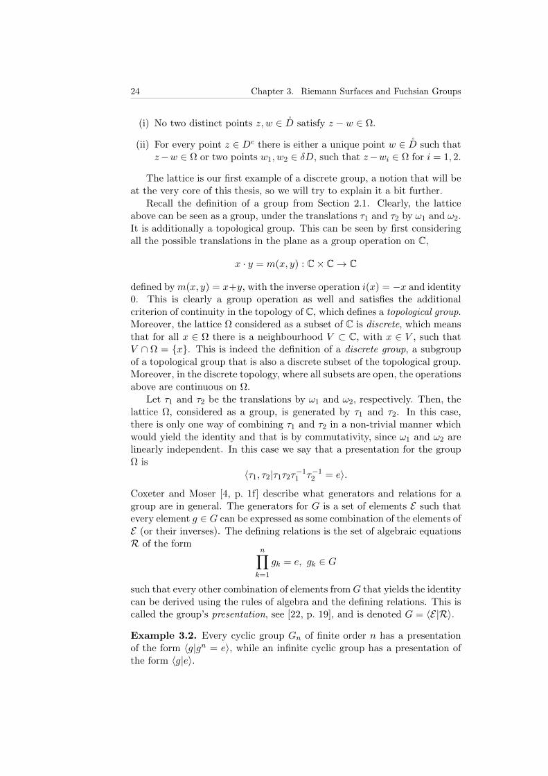
Let τ1 and τ2 be the translations by ω1 and ω2, respectively. Then, thelattice Ω, considered as a group, is generated by τ1 and τ2. In this case,there is only one way of combining τ1 and τ2 in a non-trivial manner whichwould yield the identity and that is by commutativity, since ω1 and ω2 arelinearly independent. In this case we say that a presentation for the groupΩ is
〈τ1, τ2|τ1τ2τ−11 τ−1
2 = e〉.
Coxeter and Moser [4, p. 1f] describe what generators and relations for agroup are in general. The generators for G is a set of elements E such thatevery element g ∈ G can be expressed as some combination of the elements ofE (or their inverses). The defining relations is the set of algebraic equationsR of the form
n∏k=1
gk = e, gk ∈ G
such that every other combination of elements fromG that yields the identitycan be derived using the rules of algebra and the defining relations. This iscalled the group’s presentation, see [22, p. 19], and is denoted G = 〈E|R〉.
Example 3.2. Every cyclic group Gn of finite order n has a presentationof the form 〈g|gn = e〉, while an infinite cyclic group has a presentation ofthe form 〈g|e〉.

3.2. The Euclidean Case 25
Given all the above we are now ready to construct the compact Riemannsurface associated to the lattice Ω. This is done by the topological processof quoting a space by a group. Informally, in this context, we can thinkof this process as taking out our scissors and cutting out the fundamentaldomain above and gluing together the sides that correspond to the samevector. For the lattice, then, we need to glue two pairs of sides together, asshown in Figure 3.1. In fact, this is the only way that a compact Riemannsurface arises in Euclidean geometry. Recall the definition in Section 2.2 of a
Figure 3.1: Pasting the fundamental domain for a lattice.
quotient surface. In terms of discrete groups, we now explain the definitionof a quotient surface2 X/G. Let X be a topological space and G a discretesubgroup of the automorphism group of X. Then, X/G is based on theorbits
G · x = y ∈ X : y = g · x for some g ∈ G,
which partition X into equivalence classes under the action of G. The quo-tient surface is then defined as X/G = G · x : x ∈ X. In terms of thelattice, this identifies the lattice points, in the orbit Ω + e, and for eachx 6∈ Ω, gives rise to an orbit
Ω + x = z ∈ C : z = nω1 +mω2 + x, n,m ∈ Z.
The study of fundamental domains, preferably a polygon, is connected tothe quotient spaces, since in the fundamental domain it is only the boundarypoints that are identified by the quotient. This identification is the pastingthat we described informally above and the spaces D/G and X/G coincideas sets. Thus, the problem of the study of group action on an entire spaceis reduced to the study of the action on the fundamental domain. Workingwith the identification of sides of a fundamental polygon in the case of alattice is not necessarily in need of more formalisation, but in view of thematerial ahead, we introduce the formal definition of how to pair sides for afundamental polygon D in a geometric space X, as defined in [20, p. 467],but given a slightly different notation. Let S be the set of sides of D. Then,a side-pairing for a fundamental polygon D is the set
pairs(D) = (gs, s, s∗) : s ∈ S, gs(s) = s∗,2Sometimes called the coset space G \ X, to emphasise that we are considering left
cosets. Other names are quotient space, quotient set, orbit space & c.

26 Chapter 3. Riemann Surfaces and Fuchsian Groups
where gs is an orientation-preserving isometry of X. Two sides s and s∗ aresaid to be paired if (gs, s, s
∗) ∈ pairs(D) and a vertex v of D is said to bepaired if the incident sides of v are paired by transformations gi, i = 1, 2,such that giv are vertices of D, i = 1, 2.
Now, we have not given any justification for choosing the fundamentaldomain shown in Figure 3.2a. Many other possibilities exist, but there areways to be more systematic in the way we choose a fundamental domain.There are obvious benefits to this, in terms of added structure, but in thecase of the lattice there is also a downside, since the pasting becomes lessapparent. The algorithm that we introduce for the lattice produces theDirichlet domain, since this extends in a natural, albeit not unproblematic,way to the construction of fundamental domains for Fuchsian groups. The
ω2
ω1
(a) A fundamental domain for alattice Ω built from basis vectors.
ω2
ω1
ω3
(b) The Dirichlet fundamentaldomain for a lattice Ω.
Figure 3.2: Fundamental domains for a lattice.
Dirichlet domain for a lattice Ω[13, p. 68] is defined as the set
D(Ω) = z ∈ C : |z| ≤ |z − ω| , for all ω ∈ Ω.
This means that any point is always at least as close to the origin as it isto any other lattice point. A way to construct the Dirichlet domain in analgorithmic way is to first notice that 0 ∈ D(Ω) trivially. Then, consider theline segment between 0 and ω, which we will denote by [0, ω] for all ω ∈ Ω.The z that satisfy the defining property with respect to this point lie in thehalf-plane containing 0 delineated by the perpendicular bisector of [0, ω].This would seem to be an infinite process, unless one realises that we canrestrict attention to the elements
±ω1,±ω2,±ω3, where ω3 = ω2 − ω1,
since the perpendicular bisectors of any other element are at a greater dis-tance from the origin. See Figure 3.2b and Algorithm 3.1.
This presentation is not unique, however, and it is possible to alge-braically transform the presentation for a group by Tietze transformations,described in Definition 3.5.

3.2. The Euclidean Case 27
Algorithm 3.1 Finding the Dirichlet domain for a lattice Ω.
1. Find the line segments lk,n = [0, (−1)nωk] for k = 1, 2, 3, n = 0, 1.
2. Find the perpendicular bisector of lk,n for k = 1, 2, 3, n = 0, 1.
3. Form the half-plane Hk,n bordered by lk,n such that 0 ∈ Hk,n.
4. Then, D(Ω) =⋂k,nHk,n.
Definition 3.5. [22, p. 20f] Let G = 〈E|R〉 be a group with the givenpresentation. A Tietze transformation of G is one of the following
1. Adding a generator g to E , which is derivable from the generators, to-gether with the relation gw−1 = e, where w is a word in the generatorsfrom E .
2. Supposing g ∈ E satisfies g = w with w a word in E \ g, the removal ofg and the relation gw−1 = e.
3. Adding relations that are derivable algebraically.
4. Removing relations that are derivable from the others algebraically.
Remark 3.2. The effectiveness of Tietze transformations is that two pre-sentations describe the same group if, and only if, they can be transformedinto each other by finitely many Tietze transformations. This theorem isdue to Tietze, and is the reason these transformations bear his name. More-over, we must say that this works in any group, since it is a purely algebraicprocedure, and certainly not only in C.
A way to realise such transformations geometrically is to consider do-mains that represent the different presentations and find how congruentareas can be shifted to correspond to the shift in presentation. ConsiderFigure 3.3, where the green area has been translated by ω1, the black areaby ω2 and the red area by ω1 + ω2. In the quotient there is no difference,since congruent points have been exchanged for congruent points. Movingto commutative notation, the Dirichlet domain in this case corresponds tothe presentation
〈τ1, τ2, τ3|τ1 + τ2 − τ1 − τ2 = τ1 − τ2 + τ3 = 0〉
for the lattice and the fundamental domain derived from the basis vectorscorresponds to the presentation
〈τ1, τ2|τ1 + τ2 − τ1 − τ2 = 0〉
28 Chapter 3. Riemann Surfaces and Fuchsian Groups
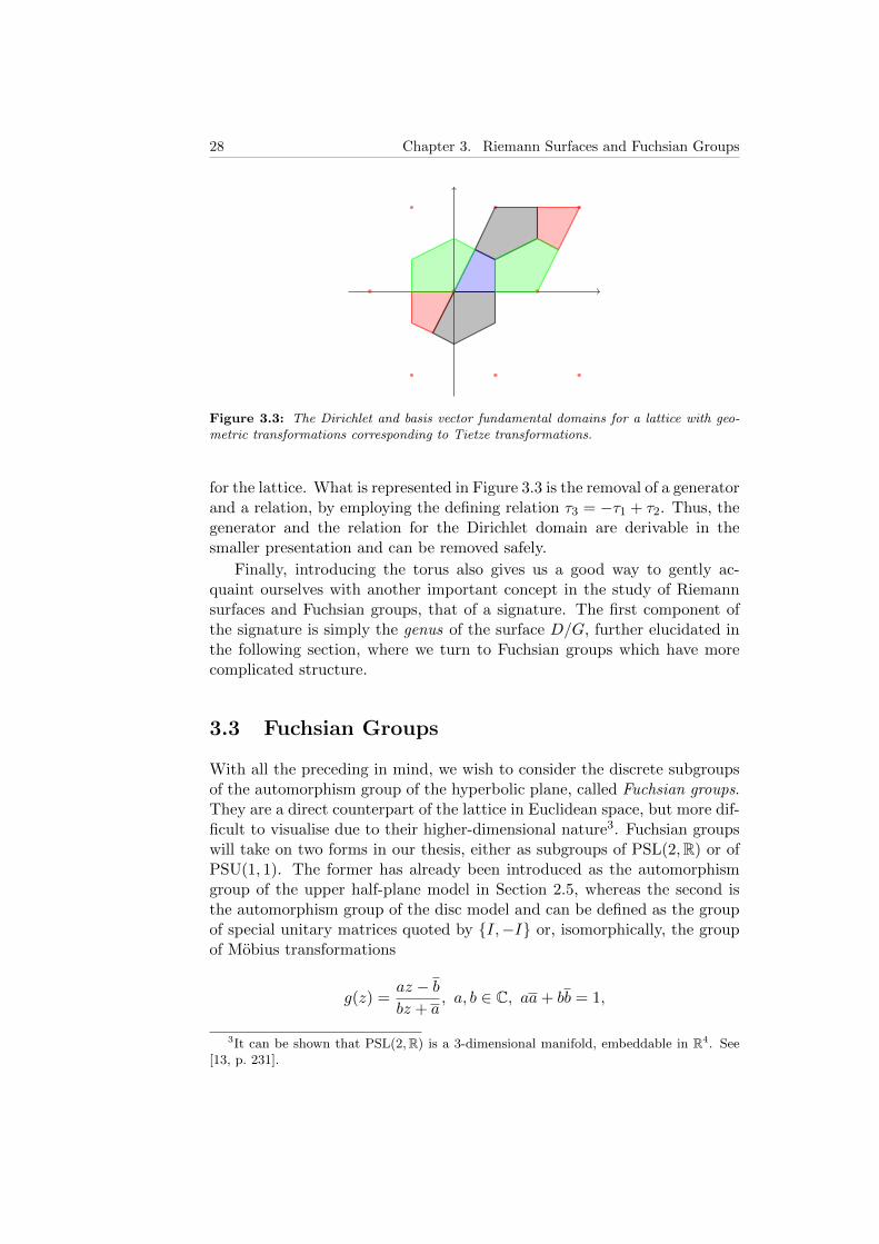
Figure 3.3: The Dirichlet and basis vector fundamental domains for a lattice with geo-metric transformations corresponding to Tietze transformations.
for the lattice. What is represented in Figure 3.3 is the removal of a generatorand a relation, by employing the defining relation τ3 = −τ1 + τ2. Thus, thegenerator and the relation for the Dirichlet domain are derivable in thesmaller presentation and can be removed safely.
Finally, introducing the torus also gives us a good way to gently ac-quaint ourselves with another important concept in the study of Riemannsurfaces and Fuchsian groups, that of a signature. The first component ofthe signature is simply the genus of the surface D/G, further elucidated inthe following section, where we turn to Fuchsian groups which have morecomplicated structure.
3.3 Fuchsian Groups
With all the preceding in mind, we wish to consider the discrete subgroupsof the automorphism group of the hyperbolic plane, called Fuchsian groups.They are a direct counterpart of the lattice in Euclidean space, but more dif-ficult to visualise due to their higher-dimensional nature3. Fuchsian groupswill take on two forms in our thesis, either as subgroups of PSL(2,R) or ofPSU(1, 1). The former has already been introduced as the automorphismgroup of the upper half-plane model in Section 2.5, whereas the second isthe automorphism group of the disc model and can be defined as the groupof special unitary matrices quoted by I,−I or, isomorphically, the groupof Mobius transformations
g(z) =az − bbz + a
, a, b ∈ C, aa+ bb = 1,
3It can be shown that PSL(2,R) is a 3-dimensional manifold, embeddable in R4. See[13, p. 231].

3.3. Fuchsian Groups 29
see [5, Theorem 23,p. 31]. As is our near-universal custom, we begin withan example.
Example 3.3. All finite subgroups of PSL(2,R) are obviously discrete. Aless trivial, but no less obvious, example is Γ, the modular group, which isthe subgroup with elements defined by
g(z) =az + b
cz + d, a, b, c, d ∈ Z, ad− bc 6= 0.
This group will play an important role in this thesis.
In the same vein as in the Euclidean case, we can construct fundamentaldomains for Fuchsian groups, that tessellate the hyperbolic plane and giverise to quotient spaces of a much richer nature than the torus. This will giveus a natural platform to introduce generalisations of many of the notionspresented in Section 3.2. However, in order to give a full picture, we firstneed to characterise the elements in PSL(2,R).
We can classify the elements of PSL(2,R) into three classes4. Each classdescribes properties in the action on the hyperbolic plane, which we willbriefly touch on and is defined by the operation trace2(g) which is equal tothe squared trace of the matrix representative of determinant 1.
Definition 3.6. [2, p. 67] Let g be a Mobius transformation with real coeffi-cients. With the above condition, we define the classification of g accordingto trace2(g):
(i) g is said to be elliptic if 0 ≤ trace2(g) < 4;
(ii) g is said to be parabolic if trace2(g) = 4;
(iii) g is said to be hyperbolic if trace2(g) > 4.
The way that these transformations act on hyperbolic space is connectedto their corresponding isometric circles, defined in Section 2.5. As presentedby Ford [5, p. 25-27], the way all the elements of the types above act is firstby inversion in the isometric circle followed by reflection in the isometricline. What differentiates them is the relation of the isometric circles Ig andIg−1 . The way to characterise the classes of elements by isometric circles isto notice that the distance between the centres of the isometric circles Igand Ig−1 is |a/c+ d/c| and the sum of radii is 2/ |c|, so that we have one ofthe three possibilities
|a/c+ d/c| ≤ 2/ |c| ,|a/c+ d/c| = 2/ |c| , or
|a/c+ d/c| ≥ 2/ |c| ,4If we would take PSL(2,C) instead, there would also exist elements with trace2(g) 6∈
[0,∞). These are called loxodromic. Some authors join hyperbolic and loxodromic ele-ments into loxodromic elements and call loxodromic elements strictly loxodromic.

30 Chapter 3. Riemann Surfaces and Fuchsian Groups
precisely corresponding to the different classes—since |a+ d| =√
trace2(g).Thus the isometric circle and the inversive isometric circle intersect, are tan-gent and are exterior to each other precisely when they are elliptic, parabolicand hyperbolic respectively.
Another frequently employed way to characterise the different elementsis in terms of their fixed points, see [13, p. 32ff]. Recall that a fixed pointof a transformation g is a z such that g(z) = z, and thus any iteration ofthe transformation will keep the point stable. The number and position offixed points characterises the different transformations. The easiest way tofind them in a particular case is simply to solve the quadratic equation
cz2 + (d− a)z − b = 0.
With a, b, c, d ∈ R, and thus working in the upper half-plane model, the onlypossibilities are two fixed points on the circle at infinity, one fixed point onthe circle at infinity of multiplicity 2 or one fixed point inside the hyperbolicplane (the “other” would have to be the complex conjugate, i.e., outside thehyperbolic plane). Simplifying the above equation yields
(2cz + (d− a))2 = (a+ d)2 − 4,
which immediately gives the characterisation as one fixed point inside thehyperbolic plane for elliptic transformations, one fixed point on the circleat infinity of multiplicity two for parabolic transformations and two fixedpoints on the circle at infinity for hyperbolic transformations.
Example 3.4. To give some examples of each type, let
g(z) = −1
z, h(z) = z + 1 and s(z) =
z + 1
z + 2,
where g is elliptic, h parabolic and s hyperbolic, with isometric circles Ig =z : |z| = 1, Ih = C and Is = z : |z + 2| = 1.
This allows us to extend the notion of a signature for a Fuchsian groupbased on the structure of the group in terms of its elliptic, parabolic andhyperbolic elements, which we shall now proceed to describe, following [13,p. 219f, 260, 262]. In this, the correspondence between the geometric view-point of fundamental domains and the algebraic viewpoint of presentationsis very tight and the viewpoints inform each other.
First of all, elliptic elements have one fixed point inside the hyperbolicplane. Thus, for any elliptic transformation, iterating the function will notmove the fixed point. Moreover, they are of finite order, by [13, Theo-rem 5.7.3.]. Thus, every elliptic element of a Fuchsian group is conjugate toan element of the form z 7→ e2πi/nz, which is a rotation of the hyperbolicdisc. This is demonstrated in Figure 3.4, with an elliptic element of order 2.

3.3. Fuchsian Groups 31
i
F
g(F )
Figure 3.4: An elliptic element gof order 2, with fixed point i, actingon a region of the hyperbolic plane,by rotation of a half turn.
The second part of the signature, whichwe started introducing in Section 3.2, isconnected to the elliptic elements. Con-sider the elliptic element g of order 2 inFigure 3.4. In general, this could be partof a larger finite cyclic group, say of or-der 4. So, it is not enough to find the el-liptic elements, which are of finite order.Instead, the objects of interest are the fi-nite cyclic subgroups of a given Fuchsiangroup, which are maximal with respect tothis property. Moreover, we can conjugatethe finite cyclic subgroups, to act with dif-ferent fixed points. Thus, we need to re-strict attention to the conjugacy classes of such maximal subgroups. If wehave orders n1, n2, . . . , nk for any representatives of the k conjugacy classes,then the signature of G is defined as sign(G) = (g;n1, n2, . . . , nk).
Now, recall that a parabolic element has its fixed point on the circle atinfinity. If we work in the upper half-plane model, this implies that the fixedpoint α ∈ R ∪ ∞. If α = ∞, then c = 0, so the Fuchsian subgroup thatfixes ∞ must be infinite cyclic. Moreover, if α ∈ R is the fixed point forg ∈ PSL(2,R), then
h(z) =1
z − α∈ PSL(2,R)
moves α to ∞, so the conjugate h g h−1 fixes ∞. Thus, all parabolicsubgroups of a given Fuchsian group are infinite cyclic. The action of aparabolic element with fixed point 0 is demonstrated in Figure 3.5a andwith fixed point ∞ in Figure 3.5b. As with the elliptic elements, in terms
0
(a) A parabolic element, withfixed point 0, acting on the hyper-bolic plane.
F g(F )
(b) A parabolic element g, withfixed point ∞, acting on a regionof the hyperbolic plane.
Figure 3.5: Parabolic elements acting in hyperbolic 2-space.

32 Chapter 3. Riemann Surfaces and Fuchsian Groups
of the signature the objects of interest are the conjugacy classes of infinitecyclic subgroups, which are maximal with respect to this property. Thedifferent infinite cyclic subgroups are, then, subgroups of the stabilisers ofdifferent points on the circle at infinity. The number of such subgroupsis the next element in the signature, so the signature of a Fuchsian groupwith genus g, conjugacy classes of maximal finite cyclic subgroups of ordersn1, . . . , nk and s conjugacy classes of maximal infinite cyclic subgroups hassignature (g;n1, . . . , nk; s).
Finally, the hyperbolic generators5 in the group determine the genus ofthe quotient surface, so that the presentation for the group with signatureas above is, by [13, p. 262],
〈h1, t1, . . . , hg, tg, e1, . . . , ek, p1, . . . , ps|en11 = · · · = enk
k
= p1 . . . pse1 . . . ekh1t1h−11 t−1
1 . . . hgtgh−1g t−1
g = e〉.
Using the signature of the group it is possible to derive a general for-mula for the area of its fundamental domain, via the Gauss-Bonnet theorem(Theorem 2.12) and the invariance of the area of a fundamental domain(Theorem 3.8). First we define the Euler characteristic.
Definition 3.7. Let G have signature (g;n1, . . . , nk; s). Then, the Eulercharacteristic is
χ(G) = (2− 2g) +k∑i=1
(1/ni − 1)− s.
Theorem 3.8. [13, Theorem 5.10.1] For any two fundamental domainsF1, F2 for a Fuchsian group G, such that δF1 and δF2 have vanishing area,the hyperbolic area µ(F1) = µ(F2).
Theorem 3.9. [13, Theorem 5.10.3, p. 262] LetG have signature (g;n1, . . . , nk; s)and let F be a fundamental domain for G, with µ(δF ) = 0. Then,
µ(F ) = −2π χ(G)
Example 3.5. The group with signature (0; 2, 3; 1) has fundamental do-mains with hyperbolic area
µ(F ) = 2π(−2 + 1/2 + 2/3 + 1) = π/3,
while the fundamental domains for the group with signature (0; 3, 3; 1) hasthe hyperbolic area,
µ(F ) = 2π(−2 + 4/3 + 1) = 2π/3.
5There is another possibility, which we will not discuss here, and that is a fundamentaldomain with boundary on the circle at infinity, corresponding to hyperbolic boundaryelements. This requires much introduction and is not relevant to the groups studied here.A full treatment can instead be found in Beardon [2].

3.4. Fuchsian Subgroups 33
The preceding example, moreover, illustrates a consequence of the factthat there is a Fuchsian group with signature (0; 2, 3; 1) with an index twosubgroup of signature (0; 3, 3; 1), because of the following theorem, calledthe Riemann-Hurwitz formula. The explicit computation of this fact is donelater, in Section 5.2.
Theorem 3.10. [13, Theorem 5.10.9(ii)] Let G be a Fuchsian group withfundamental domain F and H ≤ G, with fundamental domain Fn, such that[G : H] = n <∞. If µ(F ) <∞ and µ(δF ) = 0, then µ(Fn) = nµ(F ).
This immediately relates the Euler characteristic of a subgroup of finiteindex to that of the containing group.
Corollary 3.11. Let G be a Fuchsian group with H ≤ G and [G : H] =n <∞. Then,
χ(H)/χ(G) = n.
This directly correlates to the topic of our next section, which is thestructure of subgroups of Fuchsian groups.
3.4 Fuchsian Subgroups
Our main object in this thesis is to study the modular group and some ofits subgroups. To start with, this proposition shows that we do not have toworry in this case about proving discreteness, which, in general, can be atricky business.
Proposition 3.12. Let G be a Fuchsian group. Then, H ≤ G is a Fuchsiangroup.
Now, given a Fuchsian group of signature (g;n1, . . . , nk; s), there is away to compute the signatures of the subgroups of a given index n, usinga theorem by Singerman[17] on the structure of permutation groups. Us-ing Reidemeister-Schreier’s method, which will be described shortly, we canthen find the explicit generators of this group algorithmically as complexfunctions, only implicit in the pasting conditions for the N -sheeted coveringof the fundamental domain that is produced in Theorem 3.13.
Theorem 3.13. [17, Theorem 1] Let G be a Fuchsian group with signature
(g;m1, . . . ,mk; s),
with ej , j = 1, . . . , k, the corresponding elliptic elements of order mj , andpj , j = 1, . . . , s, the corresponding parabolic elements.
Then, G contains a subgroup GN , with [G : GN ] = N and signature
(g′;n11, . . . , n1ρ1 , . . . , nk1, . . . , nkρk ; s′)
if and only if
34 Chapter 3. Riemann Surfaces and Fuchsian Groups
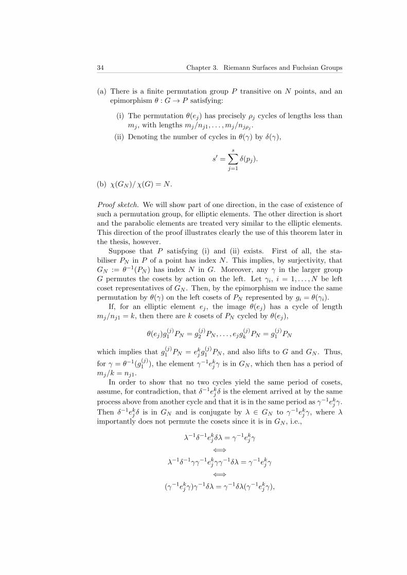
(a) There is a finite permutation group P transitive on N points, and anepimorphism θ : G→ P satisfying:
(i) The permutation θ(ej) has precisely ρj cycles of lengths less thanmj , with lengths mj/nj1, . . . ,mj/njρj .
(ii) Denoting the number of cycles in θ(γ) by δ(γ),
s′ =s∑j=1
δ(pj).
(b) χ(GN )/χ(G) = N .
Proof sketch. We will show part of one direction, in the case of existence ofsuch a permutation group, for elliptic elements. The other direction is shortand the parabolic elements are treated very similar to the elliptic elements.This direction of the proof illustrates clearly the use of this theorem later inthe thesis, however.
Suppose that P satisfying (i) and (ii) exists. First of all, the sta-biliser PN in P of a point has index N . This implies, by surjectivity, thatGN := θ−1(PN ) has index N in G. Moreover, any γ in the larger groupG permutes the cosets by action on the left. Let γi, i = 1, . . . , N be leftcoset representatives of GN . Then, by the epimorphism we induce the samepermutation by θ(γ) on the left cosets of PN represented by gi = θ(γi).
If, for an elliptic element ej , the image θ(ej) has a cycle of lengthmj/nj1 = k, then there are k cosets of PN cycled by θ(ej),
θ(ej)g(j)1 PN = g
(j)2 PN , . . . , ejg
(j)k PN = g
(j)1 PN
which implies that g(j)1 PN = ekj g
(j)1 PN , and also lifts to G and GN . Thus,
for γ = θ−1(g(j)1 ), the element γ−1ekj γ is in GN , which then has a period of
mj/k = nj1.In order to show that no two cycles yield the same period of cosets,
assume, for contradiction, that δ−1ekj δ is the element arrived at by the same
process above from another cycle and that it is in the same period as γ−1ekj γ.
Then δ−1ekj δ is in GN and is conjugate by λ ∈ GN to γ−1ekj γ, where λimportantly does not permute the cosets since it is in GN , i.e.,
λ−1δ−1ekj δλ = γ−1ekj γ
⇐⇒λ−1δ−1γγ−1ekjγγ
−1δλ = γ−1ekj γ
⇐⇒(γ−1ekj γ)γ−1δλ = γ−1δλ(γ−1ekj γ),

3.4. Fuchsian Subgroups 35
so γ−1δλ is in the centraliser of γ−1ekj γ.6 Since the centraliser is generated
by γ−1ejγ, γ−1δλ is a power of this element by some p, 1 ≤ p ≤ mj . Butthen δ−1ekj δ is in the same period as γ−1ekjγ, since
δGN = δλGN = γ(γ−1ejγ)pGN = epjγGN ,
which is a contradiction. Thus, different k-cycles give rise to different peri-ods.
A very similar argument shows that no cycle gives rise to two periods.
Example 3.6. We consider as a first example of employing this theorem thetriangle group ∆(2, 4, 6), which has one order 2 element x1, correspondingto v1 in Figure 3.6a with angle π, one order 4 element x2, correspondingto v2 with angle sum π/2, and one order 6 element x3, corresponding to v3
with angle π/3. Now, x2 = x−11 x−1
3 = (x3x1)−1, derived from the fact thata counter-clockwise turn around v2 is first employing x3 clockwise in thepasting and then x1 clockwise, i.e., with inverted orientation. This meansthat we only have two degrees of freedom in choosing the epimorphism. Sincethere are no parabolic elements, the group is of signature (0; 2, 4, 6;−).
As an aside, all triangle groups are of this form, with ∆(l,m, n) as〈x, y|xl = ym = (yx)n = e〉, and Fuchsian if 1/l + 1/m + 1/n < 1, see[17, p. 322]. In order to define an appropriate epimorphism it is enough toconsider the defining elements
θ(x1) = (1, 4)(2, 3)(5, 6), θ(x2) = (1, 6, 5, 3)(2, 4) and
θ(x3) = (1, 5, 2)(3, 4)(6).
The epimorphism was found in [12, p. 28]. We can now consider these per-mutations as pasting conditions. Take 6 copies of the triangle in Figure 3.6aand paste them according to the permutations, as shown in Figure 3.6b.Thus, when pasting the order 2 elements along the cycles of θ(x1) we getregular points, the pasting of the order 6 elements along (1, 5, 2) gives anorder 2 element, along (3, 4) an order 3 element and along 6 an order 6element, while the pasting of x2 is more difficult to see. Consider, however,that 2 and 4 share an order 2 point corresponding to the cycle (2, 4) whenpasting 1 and 2 and 3 and 4. And that 1, 3, 5 and 6 share a regular pointin the intersection of the pasting of 6 with 6 and 3 with 4. Finally, thepermutations above gives us that the signature is (g′; 2, 2, 3, 6;−) and withRiemann-Hurwitz’s condition we get g′ = 0.
Theorem 3.13 implicitly gives us the generators of the subgroup. How-ever, in order to get the Dirichlet domain and with a greater correspondencebetween fundamental domain and generators, we are interested in finding
6The subgroup consisting of all elements that commute with the given element.

36 Chapter 3. Riemann Surfaces and Fuchsian Groups
v1
v3
v2v2
(a) Pasting of a fundamentaldomain for the triangle group∆(2, 4, 6).
(b) Pasting conditions for an in-dex 6 subgroup of ∆(2, 4, 6).
Figure 3.6: Fundamental domain for triangle group with subgroup.
the generators as complex functions. This is in order to be able to ap-ply the algorithm described in Section 4.3 to the subgroups of the modulargroup which we will study and, moreover, to get a full geometric picture.This can also be done algorithmically, by the method of Reidemeister andSchreier. Here we follow the exposition in [22, Chapter 1]. Since we areonly interested in the generators, the details regarding the relations of asubgroup are not discussed and the problem reduces to that of free groups,which are abstract groups on a set of symbols, defined as the group withpresentation 〈x1, x2, . . . , xn|e〉—in the case of a finite presentation— withconcatenation of symbols as the group operation, yielding words of symbols,such as x1x2x
−11 x−1
2 . Recalling Example 3.2, we see that an infinite cyclicgroup is isomorphic to the free group on one generator—due to a theoremthat groups are isomorphic if they have the same presentation [22, Theo-rem 2.1.2]. The Reidemeister-Schreier method gives us a way to computethe generators of a subgroup as words in the generators of the group.
In order to explain this method, we must define a simple procedure topreserve uniqueness and a correspondence between words of symbols andpaths in graphs.
Definition 3.14. Let Π = v0e±11 v1e
±12 v2e
±13 v3 . . . e
±1n vn be a sequence of
directed edges ei, i = 1, . . . , n and vertices vj , j = 0, . . . , n in the di-rected graph G, such that e±1
i ends in vi and e±1i+1 starts in vi, for all
i = 1, . . . , n, with +1 denoting the normal direction and −1 the inverteddirection of the traversing of the edge. This will unambiguously be denotedΠ = e±1
1 e±12 . . . e±1
n . Then Π is said to be a path in G, and a reduced path is apath such that all occurrences of eie
−1i , so called spurs, have been removed.
Example 3.7. The path Π = e1e2e−12 e−1
1 e4 is not reduced. The corre-sponding reduced path is Π = e4. We can isomorphically consider this asreduction of a word of symbols, with inverses.
Example 3.8. We begin with an example of the Reidemeister-Schreier pro-cedure, which is easily generalised. Consider the graph representing the free
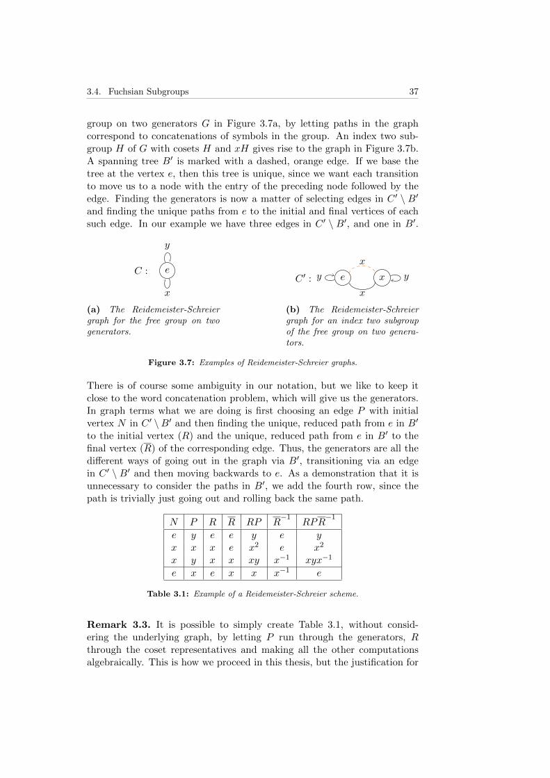
3.4. Fuchsian Subgroups 37
group on two generators G in Figure 3.7a, by letting paths in the graphcorrespond to concatenations of symbols in the group. An index two sub-group H of G with cosets H and xH gives rise to the graph in Figure 3.7b.A spanning tree B′ is marked with a dashed, orange edge. If we base thetree at the vertex e, then this tree is unique, since we want each transitionto move us to a node with the entry of the preceding node followed by theedge. Finding the generators is now a matter of selecting edges in C ′ \ B′and finding the unique paths from e to the initial and final vertices of eachsuch edge. In our example we have three edges in C ′ \ B′, and one in B′.
eC :
y
x
(a) The Reidemeister-Schreiergraph for the free group on twogenerators.
e x
x
x
C ′ : y y
(b) The Reidemeister-Schreiergraph for an index two subgroupof the free group on two genera-tors.
Figure 3.7: Examples of Reidemeister-Schreier graphs.
There is of course some ambiguity in our notation, but we like to keep itclose to the word concatenation problem, which will give us the generators.In graph terms what we are doing is first choosing an edge P with initialvertex N in C ′ \B′ and then finding the unique, reduced path from e in B′
to the initial vertex (R) and the unique, reduced path from e in B′ to thefinal vertex (R) of the corresponding edge. Thus, the generators are all thedifferent ways of going out in the graph via B′, transitioning via an edgein C ′ \ B′ and then moving backwards to e. As a demonstration that it isunnecessary to consider the paths in B′, we add the fourth row, since thepath is trivially just going out and rolling back the same path.
N P R R RP R−1
RPR−1
e y e e y e yx x x e x2 e x2
x y x x xy x−1 xyx−1
e x e x x x−1 e
Table 3.1: Example of a Reidemeister-Schreier scheme.
Remark 3.3. It is possible to simply create Table 3.1, without consid-ering the underlying graph, by letting P run through the generators, Rthrough the coset representatives and making all the other computationsalgebraically. This is how we proceed in this thesis, but the justification for

38 Chapter 3. Riemann Surfaces and Fuchsian Groups
it is not as easy to see without the complement of combinatorial graphs,however.
The previous extensive example gives the justification for the generalmethod, which is taking this approach and generalising it. The fundamen-tal requirement is the Schreier condition, which requires each coset repre-sentative to be a word in the generators of the initial group and to havethe property that each prefix in the word is a coset representative. Thiscorresponds to the fact that we want to be able to construct B′ uniquelywith edges moving us to vertices with the vertex label as the previous ver-tex label concatenated with the edge label. The algorithm is summarised inAlgorithm 3.2.
Algorithm 3.2 The Reidemeister-Schreier algorithm for finding generators.
1. Let G be a group with generators x1, . . . , xk, H ≤ G of index n, andg1, . . . , gn be coset representatives that satisfy the Schreier condition.
2. For each gi construct a vertex with label gi and for each generator xjfind the representative for the right coset Hgixj . Draw a directed edgebetween the corresponding vertices. Denote this graph C ′.
3. Construct the spanning tree B′ by selecting the unique path from e tothe vertices such that the edges in the path are concatenated to thelabel of the vertex.
4. For each edge f in C ′ \B′, concatenate the unique path in B′ from eto its initial vertex with f and the unique counter-directional path inB′ from the final vertex of f to e.
Some remarks are due, and the first one is that Reidemeister-Schreier’smethod is not in any way limited to Fuchsian subgroups, but instead is ageneral method that works for any group. Moreover, there is a duplicationin the table in Example 3.8 above. We do not need both N and R in thetable, since the Schreier condition and the construction of the spanning treeguarantees that R will be precisely N . We added this to distinguish thedifferent edges in the graph and to reduce the total amount of notation.Finally, given two complex functions g and h, the symbolic concatenationgh corresponds to the functional composition g h.
Now, we are steadily approaching the point where these theorems andalgorithms will be employed. The final step before this is to give the theoryof fundamental domains for Fuchsian groups in the next chapter.

Chapter 4
Fundamental Domains forFuchsian Groups
The question of fundamental domains was briefly touched upon in Sec-tion 3.2. Here, we will go into some detail of how this translates into therealm of Fuchsian groups.
4.1 Dirichlet and Ford Domains
Now, similar to the treatment on the lattice, we must begin by giving thedefinition of a fundamental domain for a Fuchsian group. It is instructiveto compare this with the definition for a lattice. We say that a closed set Dis a fundamental domain, [13, p. 240], for the Fuchsian group G if
(i) For each g ∈ G, no two distinct points z, w ∈ D satisfy g(z) = w. Thiscan be equivalently stated as
D ∩ g(D) = ∅
for all g ∈ G \ e.
(ii) For every point z ∈ Dc, there is a transformation g ∈ G such thatg(z) ∈ D. This can be equivalently stated as the fact that D tessellatesthe hyperbolic plane under G, i.e.,⋃
g∈Gg(D) = U or D.
Given this definition, there are several ways to construct fundamental do-mains, just as in the Euclidean case. The two standard domains we willconsider are Dirichlet domains and Ford domains. They sometimes overlapas sets, but the ways they are constructed are distinct. Both will be ofimportance in Section 4.3 and, consequently, throughout Chapter 5.
Larsson, 2015. 39

40 Chapter 4. Fundamental Domains for Fuchsian Groups
We discussed the Dirichlet domain for lattices earlier and the notion issimilar for Fuchsian groups, at least on an abstract level. The constructionof these domains, however, is not at all straight-forward, as was the case forlattices.
The Dirichlet domain, [13, p. 241], for a Fuchsian group G centred at pis the set
Dp(G) = z ∈ U : ρ(z, p) ≤ ρ(g(z), p) for all g ∈ G. (4.1)
As with the Dirichlet domain for lattices, the centre must be inDp(G) and wecould naively approach the problem of obtaining the domain algorithmicallyby a similar construction, described in Algorithm 4.1. However, the problemhere is that we are only guaranteed existence by this approach and not ageneral method of construction, since the algorithm a priori is not even cer-tain to halt. Some ways around this issue will be considered later. Existence
Algorithm 4.1 Naively finding the Dirichlet domain for a Fuchsian groupG.
1. Choose a centre p ∈ U.
2. Find the (hyperbolic) line segments lg = [p, g(p)] for g ∈ G.
3. Find the (hyperbolic) perpendicular bisector of lg for g ∈ G.
4. Form the (hyperbolic) half-plane Hg bordered by lg such that p ∈ Hg.
5. Then, D(G) =⋂g∈GHg.
of a Dirichlet domain is, then, due to the fact that ρ(z, p) ≤ ρ(g(z), p) pre-cisely describes the half-plane Hg for g and taking the intersection overall members, yields the Dirichlet domain, by definition. First of all, theDirichlet domain does not map interior points to interior points, trivially,by noticing that the interior of the domain is described by the inequalitiesρ(z, p) < ρ(g(z), p). Moreover, the hyperbolic plane is tessellated by theDirichlet domain under the elements, due to the discreteness of G implyingthe existence of an element with smallest hyperbolic distance to p, in ev-ery G-orbit over U, which thus must be in the Dirichlet domain. (See [13,Theorems 3.1.3, 3.4.5,p. 241].)
In the special case of a finite group, however, we can employ the abovemethod directly.
Example 4.1. Two of the smallest Fuchsian groups are the cyclic groupsgenerated by −1/z and −1/(z + 1), of order 2 and 3 respectively. Theirrespective fundamental domains are presented in this example as illustrationof the naive approach.

4.1. Dirichlet and Ford Domains 41
(i) We first consider the finite group consisting of the elements e(z) = zand g1(z) = −1/z. We first choose the centre of the Dirichlet domainas p = 2i. Then, g1(2i) = i/2, so that the hyperbolic perpendicularbisector of the line segment [i/2, 2i] is the upper half of the unit circle,since the point of intersection between the imaginary axis and thebisector is iy, y > 0, where ρ(i/2, iy) = ρ(2i, iy) is fulfilled. This isequivalent, by Theorem 2.11, to the equation
ln(y/(1/2)) = ln(2/y).
Moreover, the perpendicularity condition forces the centre of the circleto be the origin. Thus, the fundamental domain for the group is dis-played in Figure 4.1a. The reader should however not be deceived bythe Euclidean intuition that the area in the interior of the displayedcircle is finite. Every fundamental domain for a Fuchsian group hasthe same invariant area (assuming that the boundary has vanishingarea), see Theorem 3.8, which in this case is infinite.
(ii) For the group consisting of e(z) = z, g1(z) = −1/(z + 1) and g2(z) =−(z+ 1)/z, we once again choose p = 2i as our centre. In Figure 4.1b,the geodesics connecting the images of 2i under g1 and g2 are drawnin blue and the perpendicular bisectors in black.
2i
i/2
(a) Fundamental domain for acyclic Fuchsian group of order 2.
2i
(b) Fundamental domain for acyclic Fuchsian group of order 3.
Figure 4.1: Fundamental domains for finite Fuchsian groups.
A more interesting case is the modular group, Γ, which is generated byboth of the two elements −1/z and −1/(z + 1), given in Example 4.1.
Example 4.2. [13, p. 242-244] The Dirichlet domain centred at ki, k > 1,for Γ is the intersection of the hyperbolic half-planes given by the perpen-dicular bisectors of [ki, ki+ 1], [ki, ki− 1] and [ki, i/k], i.e., bounded by thevertical lines Re(z) = −1/2, Re(z) = 1/2 and the segment between theselines of the unit circle, seen in Figure 4.2. This immediately implies thatthe Dirichlet domain for Γ centred at ki is a subset of this set. The otherinclusion is shown by the reflective symmetry of the Dirichlet domain cen-tred at ki around the imaginary axis, i.e., z ∈ Dki(Γ) implies −z ∈ Dki(Γ).

42 Chapter 4. Fundamental Domains for Fuchsian Groups
Define the reflection r(z) = r−1(z) = −z, which is an isometry. For anyg ∈ Γ, r g r−1 ∈ Γ and by the invariance of the hyperbolic metric underisometries,
ρ(r(z), ki) = ρ(z, ki) ≤ ρ(r−1(g(r(z))), ki) = ρ(g(r(z)), ki),
so −z must also be part of Dki(Γ). The next step in the process is to showthat if a transformation of Γ takes a point z of F to another point w of F ,then both z and w must be boundary points and either has z as a fixed pointor takes z to its mirror image in the imaginary axis, w = −z. By combiningthis with the above, the result will be fairly immediate. We begin with theconclusion however, since this will give the motivation for taking this step.Assume that g ∈ Γ takes z ∈ F to w ∈ F , then by the following, they willboth be on the boundary of F and either
w = z =⇒ ρ(z, ki) = ρ(g(z), ki),
orw = −z =⇒ ρ(z, ki) ≤ ρ(g(z), ki),
by the above. This will thus establish the inclusion. Now, let
g(z) =az + b
cz + d, ad− bc = 1, with a, b, c, d ∈ Z,
such that g 6= e and consider the points z and w = g(z), both in F . Firstof all, we want to establish that the imaginary parts of z, w are the same.Since w ∈ F ,
|cz + d|2 = c2 |z|2 + 2cdRe(z) + d2 ≥ c2 − cd+ d2 = (c− d)2 + cd ≥ 1,
using the penultimate expression when cd ≤ 0 and the final expressionwhen cd > 0, to establish the inequality. This immediately implies thatIm(w) ≤ Im(z) and by exchanging for g its inverse, we obtain the equalityof imaginary parts and, since
Im(w) = Im(z)/ |cz + d|2
also the equality |cz + d|2 = 1. Then we also obtain the enclosure
0 ≤ cd ≤ 1,
by considering the two equalities that follow, together with the integralityof c, d:
(c− d)2 = 1− cd(c+ d)2 = 1 + 3cd.
This gives us three possibilities.
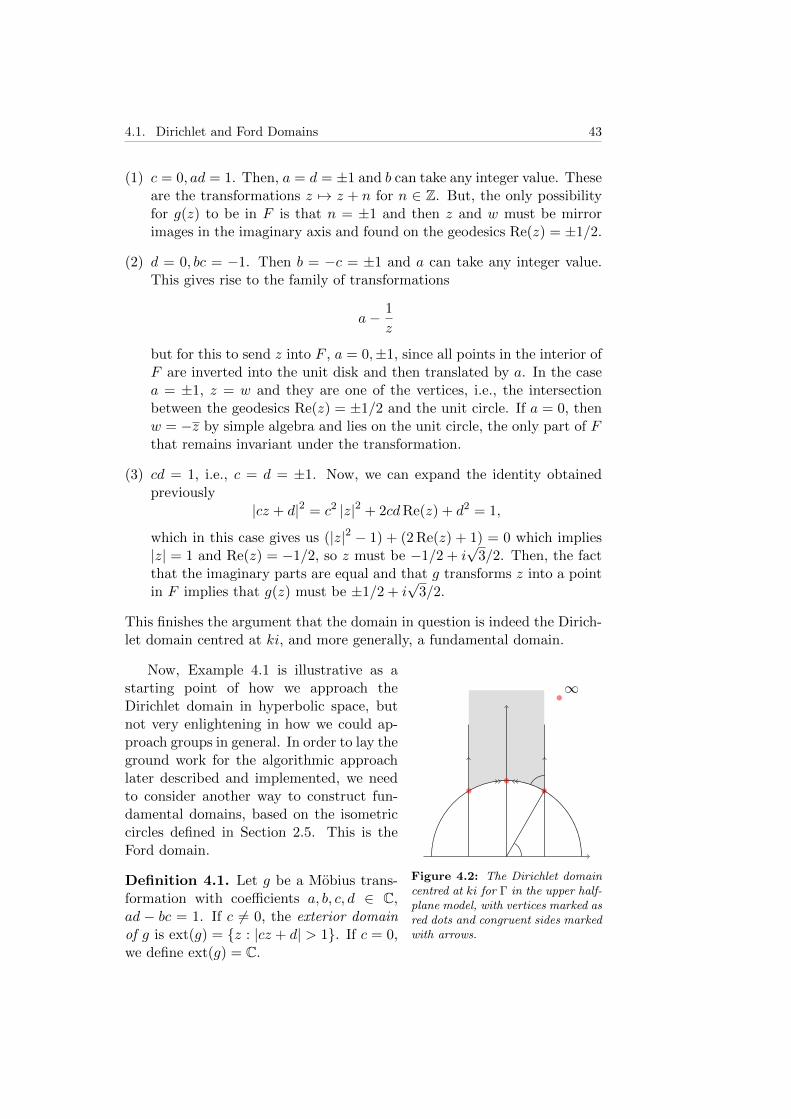
4.1. Dirichlet and Ford Domains 43
(1) c = 0, ad = 1. Then, a = d = ±1 and b can take any integer value. Theseare the transformations z 7→ z + n for n ∈ Z. But, the only possibilityfor g(z) to be in F is that n = ±1 and then z and w must be mirrorimages in the imaginary axis and found on the geodesics Re(z) = ±1/2.
(2) d = 0, bc = −1. Then b = −c = ±1 and a can take any integer value.This gives rise to the family of transformations
a− 1
z
but for this to send z into F , a = 0,±1, since all points in the interior ofF are inverted into the unit disk and then translated by a. In the casea = ±1, z = w and they are one of the vertices, i.e., the intersectionbetween the geodesics Re(z) = ±1/2 and the unit circle. If a = 0, thenw = −z by simple algebra and lies on the unit circle, the only part of Fthat remains invariant under the transformation.
(3) cd = 1, i.e., c = d = ±1. Now, we can expand the identity obtainedpreviously
|cz + d|2 = c2 |z|2 + 2cdRe(z) + d2 = 1,
which in this case gives us (|z|2 − 1) + (2 Re(z) + 1) = 0 which implies|z| = 1 and Re(z) = −1/2, so z must be −1/2 + i
√3/2. Then, the fact
that the imaginary parts are equal and that g transforms z into a pointin F implies that g(z) must be ±1/2 + i
√3/2.
This finishes the argument that the domain in question is indeed the Dirich-let domain centred at ki, and more generally, a fundamental domain.
∞
Figure 4.2: The Dirichlet domaincentred at ki for Γ in the upper half-plane model, with vertices marked asred dots and congruent sides markedwith arrows.
Now, Example 4.1 is illustrative as astarting point of how we approach theDirichlet domain in hyperbolic space, butnot very enlightening in how we could ap-proach groups in general. In order to lay theground work for the algorithmic approachlater described and implemented, we needto consider another way to construct fun-damental domains, based on the isometriccircles defined in Section 2.5. This is theFord domain.
Definition 4.1. Let g be a Mobius trans-formation with coefficients a, b, c, d ∈ C,ad − bc = 1. If c 6= 0, the exterior domainof g is ext(g) = z : |cz + d| > 1. If c = 0,we define ext(g) = C.
44 Chapter 4. Fundamental Domains for Fuchsian Groups
LetG ≤ PSU(1, 1) = pPSL(2,R) p−1, be a set of Mobius transformationsacting on D, with p one of the homeomorphisms described in Example 2.3.Then, the exterior domain of G is
ext(G) =⋂g∈G
ext(g) ∩D.
If G, moreover, is a Fuchsian group acting on the hyperbolic disc, then theexterior domain, as defined here, is called the Ford domain for G.
That the Ford domain is a fundamental domain is established by Ford in[5, p. 44-46, 67]. The method is more general than for Fuchsian groups andconsiders all groups that work on the extended complex plane Σ. The extraproperty of Fuchsian groups is that the common fixed circle, also called theprincipal circle by Ford, of all such groups is the boundary of a model ofthe hyperbolic plane, which corresponds to the fact that they are subgroupsof the automorphism group of the hyperbolic plane. Furthermore, [5, The-orem 1, p. 67] gives us that the isometric circles of a Fuchsian group areorthogonal to the boundary of the hyperbolic plane, i.e., they are geodesics.This implies that if we consider the isometric circles and δD as subsets of Σ,then inversion in δD will carry the Ford domain, as a domain in Σ, into itselfand the interiors of isometric circles into themselves. Thus, all results arevalid if we only consider the hyperbolic disc model, and by homeomorphism,the upper half-plane model.
We proceed in the more general manner, considering the domain with-out the intersection with D. Briefly, transformations map the exterior oftheir isometric circle into the interior of the isometric circle of the inversetransformation, which means that condition (i) for a fundamental domainis fulfilled. Showing that any point in the hyperbolic plane is congruentto a point of the Ford domain is a lengthier process, involving a proof bycontradiction, which we will only sketch. First consider a circle C with nopoints of the Ford domain nor points congruent to it, centred at z0 ∈ C.Then, z0 is either in the interior or on the boundary of an isometric circle Igof a transformation g, which by extension must be true of the entire orbit ofz0 under the group in question. Since all transformations map the centres oftheir isometric circles to ∞, which is in the domain, the orbit of z0 can notcontain any such centres. Using some knowledge of the action of elementsin relation to their isometric circles, briefly touched upon in Section 3.3, aniterative scheme arises that generates a transformation of C of arbitrarilylarge radius, which is a contradiction of the assumption that C contained nocongruent points, since the radii of isometric circles are bounded from above,by [5, p. 41]. Thus, the Ford domain also satisfies the second requirementof fundamental domains, by the general method and by the remarks on howto restrict ourselves to Fuchsian groups.

4.2. Sides and Vertices on Fundamental Polygons 45
Remark 4.1. Using the disc model is potentially much easier conceptuallythan the upper half-plane model when considering Ford domains, since wedo not have the point∞ to consider, but can work with only circles and neednot consider generalised circles. Including groups with a fixed point at ∞takes extra care, and a further exposition of this is detailed in [5, p. 75-78].
The final theorem that connects the two domains and makes the algo-rithm which we present in Section 4.3 effective is the following.
Theorem 4.2. [20, p. 471] Let G ≤ PSU(1, 1) be a Fuchsian group actingon D. Then, D0(G) = ext(G).
4.2 Sides and Vertices on Fundamental Polygons
One of the reasons that fundamental polygons are so interesting is the closecorrespondence of the characteristics of the polygon and how the group actson its vertices and sides on the one hand and the algebraic presentationon the other. In this section, we will describe this connection further bypresenting and illustrating Poincare’s side-pairing theorem. Recall fromSection 3.2 the definition of a side-pairing, i.e., two sides s and s∗ of apolygon are paired by an element g ∈ G if g(s) = s∗. If we have a pairing ofall the sides in a polygon, all the vertices are also paired by these elements.The following is a summary of [13, p. 245-247, 255]
Example 4.3. Consider the fundamental domain for Γ in Figure 4.2. Thevertical sides are paired by g(z) = z + 1 and the circle segment is pairedto itself by h(z) = −1/z. The vertices are, moreover, fixed by differentelements. The ideal vertex ∞ is fixed by g, while the vertex i is fixed by hand the vertices −1/2+i
√3/2 and 1/2+i
√3/2 are fixed by s(z) = −1/(z+1)
and g s g−1(z) = (z − 1)/z.
The preceding example gives us occasion to discuss several general pat-terns that are demonstrated there. First of all, we define an elliptic vertexas a vertex that is fixed by an elliptic element. In the side-pairing it will bepart of a cycle of vertices that are all elliptic, since if g maps s to s∗ andv1 ∈ s is fixed by the elliptic element e1, then g(v1) ∈ s∗ is fixed by theelliptic element g e1 g−1. The angle sum of such a cycle corresponds tothe order of the group generated by any element fixing one of the vertices:there is a conjugacy class of maximal finite cyclic subgroups of order n if,and only if, there is a corresponding cycle of elliptic vertices with angle sum2π/n, see [2, Theorem 9.3.5].
Moreover, the ideal vertex∞ is fixed by g. Since g is a parabolic element,∞ is called a parabolic vertex. The angle at such a vertex is defined as 0.
Finally, there is a point which we called a vertex in Example 4.3 whichis not a vertex in the normal sense. The reason is that it is the fixed point

46 Chapter 4. Fundamental Domains for Fuchsian Groups
of an order two elliptic element, namely −1/z. Such elements pair sidesto themselves and their fixed point is on the side. One can thus considerthe fixed point as a vertex and the side as two sides, or alternatively, allowself-pairings.
In the above, we have gone from the group to the geometry. The the-orem of Poincare also reverses this process, so that under certain naturalconditions, one moves backwards to receive a group by its generators andrelations from a given polygon and pairings. This means that there is atwo-way correspondence between algebra and geometry.
Theorem 4.3. [2, Theorem 9.8.4] Let P be a hyperbolic polygon with side-pairing pairs(P ) and let G be the group generated by the pairing elementsgs in pairs(P ). If,
(i) for each vertex v of P , there are vertices v0, v1, . . . , vn of P and el-ements f0, . . . , fn of G which constitute a cyclic pairing of sides, i.e.,fj+1 = gs fj , with v0 = v and f0 = fn+1 = e, and
fj(y ∈ P : ρ(y, vj) < ε
)are non-overlapping and forms the union B(v, ε).
(ii) ε can be chosen independently of v in P ,
then G is a Fuchsian group and P is a fundamental polygon for P .
Remark 4.2. This somewhat technical theorem can in many cases berephrased as a set of side and angle sum conditions, see [19, p. 170, 180].
Example 4.4. The fundamental domain Dki(Γ) for Γ has side-pairing el-ements g(z) = z + 1 and h(z) = −1/z. By Poincare’s theorem the groupgenerated by g and h is Fuchsian and has P for fundamental domain. Thisgroup is, naturally, Γ.
4.3 Algorithmic Computation of Fundamental Do-mains
Since the problem of finding the Dirichlet domain in general is non-trivial, asseen in Example 4.2, it is interesting to note that in certain cases, using somespecial structures it is possible to calculate it explicitly using an algorithmicapproach. One such approach is the one studied by John Voight in [20]. Thisalgorithm is based on certain assumptions, that in general, can be difficultto determine, but in specific and interesting cases are known to hold. Hismain theorem is, in a somewhat simplified form,

4.3. Algorithmic Computation of Fundamental Domains 47
Theorem 4.4. Let G be a Fuchsian group generated by a known finite set,whose members have coefficients in an algebraic field extension of Q andsuppose that G is a cofinite group, i.e., its fundamental domain has finitearea. Moreover, let p ∈ U not be fixed by any element in G\I. Then, thereis an algorithm which returns the Dirichlet domain DG(p), a side-pairing ofDG(p) and a minimal finite presentation for G.
This approach is useful for instance in the case of a large class of Fuchsiangroups called arithmetic, which are known to be cofinite, but which we willnot go into here. But, as will be apparent later, when we study the modulargroup and its subgroups, this method is useful in this case as well.
Remark 4.3. If we have a group like the modular group, which acts on U,we need to conjugate it first to act on D, in order for the algorithms in thischapter to work. See Section 3.3.
We need a few new concepts to systematically find Dirichlet domains,but we begin with a birds-eye view of the process.
1. If H ⊂ G is finite, then we can compute a normalised boundary of
E = ext(H).
2. Given a finite subset H ⊂ G, we can reduce every element γ ∈ G withrespect to H.
3. Using the known relation 〈H〉 = G, we can find a normalised basis forG, by reduction.
Now, the above summary introduces many undefined concepts, whichwe will now begin to unravel. First of all, the normalisation concepts areclearly intertwined.
Definition 4.5. A normalised basis H for a group G is a generating setfor G, such that ext(H) is a fundamental domain for G, and that forms anormalised boundary for ext(H). Now, a normalised boundary for a domainD = ext(H) is a sequence
U = (g1, g2, . . . , gn)
such that (i) D = ext(U); (ii) Ig1 , . . . , Ign contain the counterclockwiseconsecutive sides of D; (iii) the vertex v ∈ D with minimal argumentarg(v) ∈ (0, 2π), where v is considered as a complex number, is either aproper vertex of the meet of Ig1 and Ig2 or an ideal vertex with v ∈ Ig1 .
This is enough to take care of the first step in the process. The input isH ⊆ G finite. The output is a normalised boundary U of ext(H) in D. Wemake sure we find the vertices in cyclic order so that the argument of thevertex in each subsequent step is minimised. This will yield a sequence thatsatisfies the above definition.

48 Chapter 4. Fundamental Domains for Fuchsian Groups
Algorithm 4.2 Finding a normalised boundary for ext(H).
1. Initialise θ := 0, U := ∅ and L := [0, 1].
2. Let B be the set of g ∈ H such that arg(Ig ∩ L) ≥ θ.
If B = ∅, choose g ∈ H that minimises the argument of the initialvertex of Ig in [θ, θ + 2π).
Else, choose g ∈ B that minimises the argument of the meet of Igand L in [θ, θ + 2π), such that the meeting angle is minimal.
3. If g ∈ U , return the normalised boundary U .
Else update U by appending g, L := Ig ∩ D, θ to the minimalargument found in 2. Go to step 2.
Example 4.5. Finding the normalised boundary for an exterior domain isexemplified in Figure 4.3, where the boundary is taken counter-clockwisefrom the point 1 in the complex plane.
1
Figure 4.3: Example of a nor-malised boundary.
The second step is the reduction pro-cess, which is the core process that allowsus to reduce the problem of computing afundamental domain to an algorithm in fi-nite time. Recall the naive approach givenin Algorithm 4.1, which, in comparison, isnot guaranteed to end in finite time. Thisrequires an introduction of the map
r : G→ R+,
which is defined for groups acting on D by
γ 7→ r(γ; z) = ρ∗(γ(z), 0).
We then say that an element γ ∈ G is (H, z)-reduced if, for a fixed z ∈ Dand for all g ∈ H, r(g γ; z) ≤ r(γ; z) and H-reduced if z = 0.
The reduction algorithm in Algorithm 4.3 takes as input an orderedset H ⊂ G \ I, γ ∈ G, and z ∈ D and returns two group elements,redH(γ; z) ∈ G and δ ∈ 〈H〉, such that redH(γ; z) is (H, z)-reduced andredH(γ; z) = δ γ. If z = 0, we abbreviate redH(γ; 0) = redH(γ). Reducingγ in this way is a straight-forward iteration, where halting is ensured by thediscreteness of G.

4.3. Algorithmic Computation of Fundamental Domains 49
Algorithm 4.3 Computing redH(γ; z) = δ γ.
1. Initialise γ := γ and δ := e.
2. Compute r := r(γ; z) and for each gi ∈ H, compute ri := r(giγ; z) and,then, compute r := mini ri.
If r ≤ r, then return redH(γ; z) = γ and δ.
Else let g := gi be such that ri = r and for any rj = r, i ≤ j.
3. Update γ := g γ and δ := g δ. Go to step 2.
Example 4.6. Let H be the set of transformations
g1(z) =(1 + i/2)z − i/2iz/2 + 1− i/2
, g−11 (z) =
(1− i/2)z + i/2
−iz/2 + 1 + i/2,
g2(z) =(1− 2i)z − 2i
2iz + 1 + 2i, g−1
2 (z) =(1 + 2i)z + 2i
−2iz + 1− 2i,
then the reduction algorithm above, which is easily verified, yields that thereduction redH\g1(g1; 0) = e(z), with δ(z) = g−1
1 (z). This corresponds to
the fact that g1 is in any group with g−11 as a generator.
This makes it possible to construct a normalised basis for 〈H〉, and thusif we know a finite generating set for G, we can construct a normalisedbasis for G. Algorithm 4.4 is, in essence, a matter of finding a normalisedboundary for the exterior domain of the generators and their inverses, andthen successively adding elements to use for the exterior domain until thedomain has a side-pairing. There is a slight clarification in Step 5 comparedwith the article. This clarification has been made in private correspondencewith the article author.
For computational purposes, we employed C++ together with the GiNaC
library, see [7]. Common functionality is found in Appendix A.1, the im-plementation of Algorithm 4.3 in Appendix A.2 and finding approximatepairings for step 5 of Algorithm 4.4 in Appendix A.3. Since the GiNaC li-brary does not support symbolic square roots out of the box, any plausiblepairings were double-checked with Wolfram|Alpha, see [21].
One of the main objectives of this thesis is using this algorithm forsubgroups of a particular Fuchsian group, which was introduced earlier,the modular group. In order to start our investigation, we will turn to themodular group, Γ, and compute a fundamental domain for this group.

50 Chapter 4. Fundamental Domains for Fuchsian Groups
Algorithm 4.4 Computing a normalised basis for 〈H〉.As input we take an ordered setH = (g1, . . . , gt). LetH−1 := (g−1
1 , . . . , g−1t ).
1. Update H := H ∪H−1.
2. Compute the normalised boundary U of ext(H) by Algorithm 4.2.
3. Let H ′ := U . For each g ∈ H, compute g = redH\g(g) using Algo-rithm 4.3. If g 6= e, update H ′ := H ′ ∪ g.
4. Compute the normalised boundary U ′ of ext(H ′).
- If U ′ = U , then set H := H ′. Go to step 5.
- Else set U := U ′. Go to step 3.
5. Let E := ext(U) and let V be the set of vertices of E not paired byelements in H.
- If V = ∅, then return the normalised boundary U .
- Else, for each gk ∈ H, such that vk ∈ V ∩ Igk , compute
gk := redH(gk; vk), k = 1, . . . ,m.
For ideal vertices, the reduction is instead made on a point in Igk thatis hyperbolically closer to Ig−1
k\ E.
Update H := H ∪⋃nk=1 gk and go to step 2.
Chapter 5
Computations for SpecificFuchsian Groups
Turning to concrete computations, we will consider the modular group Γ,its only index 2 subgroup, its two index 3 subgroups and another type ofsubgroup, which is of index 6.
5.1 The Modular Group Γ
The first concrete group that we shall consider in more depth is the modulargroup, which, the reader will recall, is the subgroup of PSL(2,R) which hasthe further constraint that its coefficients are limited to the integers. Thus,it is denoted PSL(2,Z), but more briefly Γ, and can be defined as the set ofMobius transformations,
g(z) =az + b
cz + d, a, b, c, d ∈ Z, ad− bc 6= 0.
As a consequence of Example 4.4, this group is generated by the functions,
s(z) = z + 1 and t(z) = −1/z.
Using the knowledge of these generators, we can compute the fundamentaldomain algorithmically.
The first step is to conjugate the two generators s and t to act on Dinstead of U. In order to do this, we must first choose an appropriate home-omorphism, so that our choice of centre is mapped onto 0 of D, since thealgorithm generates a Dirichlet domain with centre 0 of the disc model. Inorder for the algorithm to work, we need to have a trivial stabiliser of thecentre. Now, take g ∈ Γ. Then, for k > 1,
g(ki) =aki+ b
cki+ d=bd+ ack2 + ki
c2k2 + d2= ki
Larsson, 2015. 51

52 Chapter 5. Computations for Specific Fuchsian Groups
is equivalent to the system of equations, together with the requirement onthe determinant,
bd+ ack2 = 0
c2k2 + d2 = 1
ad− bc = 1
If c = 0, then b = 0, d = ±1, a = d, so g(z) = z. If c 6= 0, however,c2k2 > c2 ≥ 1, since k > 1, so no such element can satisfy the secondequation. Thus, ki is not fixed by any non-trivial element of Γ.
Choose k = 2 and conjugate the matrix representatives of s and t asfollows.
g1 := p s p−1 =
(1 −2i1 2i
)(1 10 1
)(1/2 1/2i/4 −i/4
)=
(1 + i/4 −i/4i/4 1− i/4
),
g2 := p t p−1 =
(1 −2i1 2i
)(0 −11 0
)(1/2 1/2i/4 −i/4
)=
(−5i/4 −3i/43i/4 5i/4
).
It is trivial to show that such a conjugation indeed gives generators forthe conjugate group. Per Algorithm 4.4, we let H := (g1, g2, g
−11 , g−1
2 ),where g−1
1 = g1 and g−12 = −g2. Next, we must compute the normalised
boundary of ext(H) and this requires us to compute the isometric circlesof the elements of H. The reader is encouraged to follow the process bysimultaneously viewing Figure 5.1. The isometric circles are
Ig1 = z : |z − 1− 4i| = 4, Ig2 = z : |z + 5/3| = 4/3,Ig−1
1= z : |z − 1 + 4i| = 4, Ig−1
2= Ig2 .
The final equality is due to the fact that g2 = g−12 as transformations,
and by projective identification of the matrix representatives. As stated inAlgorithm 4.2 we initialise θ := 0, U := ∅ and L := [0, 1].
1. The only isometric circle that intersects L with argument greater thanor equal to 0 is Ig1 , so we update U := (g1), L := Ig1 ∩D and θ := 0.
2. The only isometric circle that intersects L with argument greater than orequal to 0 is Ig2 , so we update U := (g1, g2), L := Ig2 ∩D and θ ≈ 2.5536.
3. The only isometric circle that intersects L with argument greater thanor equal to θ is Ig−1
1, so we update U := (g1, g2, g
−11 ), L := Ig−1
1∩D and
θ ≈ 3.7296.
4. Finally, we would get Ig1 again. But, then we are done and the algorithmreturns the normalised boundary (g1, g2, g
−11 ).

5.2. The Index Two Subgroup of Γ 53
Then, we let H ′ := (g1, g2, g−11 ). We compute the reductions
g1 = e, δ1 = g−11 , g2 = e, δ2 = g−1
2
g−11 = e, δ−1
1 = g1, g−12 = e, δ−1
2 = g2.
Since all reductions are the identity, there is nothing to add to H ′ andtrivially the normalised boundary of ext(H ′) is U . Thus, we update Hto (g1, g2, g
−11 ). The vertices of ext(U) are v1 = 1, v2 = (6
√3−15− i(4
√3−
10))/13 and v3 = v2. Now,
g1(v1) = g−11 (v1) = v1, g1(v2) = v3 and g−1
1 (v3) = v2,
so all sides are paired and there is no need for further iterations. Since allMobius transformations are conformal, the mapping of the three verticesunder p−1 is enough to establish the domain in the upper half-plane,
p−1(v1) =∞, p−1(v2) =−1 + i
√3
2and p−1(v3) =
1 + i√
3
2,
which is familiar, since this is precisely the domain displayed in Figure 4.2.
5.2 The Index Two Subgroup of Γ
v1
v2
v3
Ig1
Ig−11
Ig2
Figure 5.1: The isometric circlesof g1, g2 and g−1
1 and their exte-rior domain with normalised bound-ary for Γ.
Our next object of investigation is the firstof the subgroups of the modular group: theone of index two, i.e., that splits the modu-lar group in two cosets. We will show thatthere is only one such group, by employingthe theorem described in Section 3.4. Theproblem of finding all such subgroups re-duces to constructing the possible epimor-phisms θ : Γ → C2, where C2 is the cyclicpermutation group on two elements.
Given the presentation of Γ, which is〈x, y|x2 = y3 = e〉, there are only two possi-bilities that determine the epimorphism en-tirely. The first possibility is θ(x) = (1, 2)and θ(y) = (1)(2), where thus θ(xy) =(1, 2). Now, the signature of Γ is (0; 2, 3; 1). Then, by applying Theo-rem 3.13, θ(x) has 1 cycle of length 2 ≤ 2 for x, 2 cycles of length 1 ≤ 3 fory and for the parabolic element xy one cycle of length 2. The only stabiliserof points in this group is the trivial one. So θ−1((1)(2)) = ker(θ) hasthe signature (g′; 3, 3; 1). From now on, we will use the simplifying notationG2 := ker(θ). From the relation [G : H] = χ(H)/χ(G) for H ≤ G, we get
χ(G2) = 2g′ − 2 +2
3+
2
3+ 1 = 2 · χ(Γ) =
1
3,

54 Chapter 5. Computations for Specific Fuchsian Groups
so g′ = 0. Thus, the signature of this group is sign(G2) = (0; 3, 3; 1).If we follow Jones & Singerman [13] in the Tietze transformation of
the presentation, and the corresponding fundamental domain in Figure 4.2,whereby the part of the domain with −1/2 ≤ Re z ≤ 0 is moved to 1/2 ≤Re z ≤ 1, a geometric view of the subgroup in hyperbolic space is easierto see. The order 2 element corresponding to the vertex at i has beeneliminated, and thus a turn around the point in the quotient space is a fullcircular rotation, and the point is thus regular, indicated by green points.However, the order 3 elements have been duplicated, thus yielding the conepoints, indicated by red points.
∞
Figure 5.2: A fundamental do-main for the index two subgroup ofΓ, constructed by the implicit past-ing conditions of the constructionfrom Singerman’s theorem.
If we try to use the other possible epi-morphism, with θ(x) = (1)(2) and θ(y) =(1, 2), it does not satisfy the cycle condi-tions, since we need the orders of the groupmj to be divisible by the cycle lengths ck,
mj/nj,k = ck ⇐⇒ mj/ck = nj,k.
Further, in order to algorithmically pro-duce a fundamental domain we need to findthe generators of the subgroup, by applyingthe Reidemeister-Schreier method. This re-quires us to consider the group Γ abstractlyas a set of words in the symbols x and ywith the presentation above, which we re-call is 〈x, y|x2 = y3 = e〉. As previously stated in Section 3.4 we only need toconsider the free group on the generators of Γ in order to find the generatorsof the subgroup, i.e., the group S = 〈x, y|e〉.
Now, consider Table 5.1, where we let R run through the right cosetrepresentatives of G2 and P through the generators of Γ, by Remark 3.3.
R P R RP R−1
RPR−1
e x x x x−1 ee y e y e yx x e x2 e ex y x xy x−1 xyx−1
Table 5.1: Reidemeister-Schreier scheme for G2 ≤ Γ.
According to the Reidemeister-Schreier method, the final column is thena listing of the generators of G2, which is thus generated by the two elements,
s(z) = − 1
z + 1, t(z) =
z − 1
z.
The observant reader will spot that t(s(z)) = z + 2, which should be ex-pected from the domain shown previously in Figure 5.2 and which gives the

5.2. The Index Two Subgroup of Γ 55
alternative generators s and ts. Since G2 ≤ Γ, we already know that p = 2iis fixed by no element of G2, so no problem arises if we use this point asour centre for the Dirichlet domain. Thus, we conjugate the matrices, as inSection 4.3,
g1 := p s p−1 =
(1 −2i1 2i
)(0 −11 1
)(1/2 1/2i/4 −i/4
)=
(1/2− 5i/4 −1/2− 3i/4−1/2 + 3i/4 1/2 + 5i/4
),
g2 := p t p−1 =
(1 −2i1 2i
)(1 −11 0
)(1/2 1/2i/4 −i/4
)=
(1/2− 5i/4 1/2− 3i/41/2 + 3i/4 1/2 + 5i/4
).
We let H := (g1, g2, g−11 , g−1
2 ), where
g−11 =
(1/2 + 5i/4 1/2 + 3i/41/2− 3i/4 1/2− 5i/4
)and g−1
2 =
(1/2 + 5i/4 −1/2 + 3i/4−1/2− 3i/4 1/2− 5i/4
).
Thus, the isometric circles are
Ig1 = z : |z + 11/13− 16i/13| = 4√13,
Ig2 = z : |z + 19/13 + 4i/13| = 4√13,
Ig−11
= z : |z + 19/13− 4i/13| = 4√13,
Ig−12
= z : |z + 11/13 + 16i/13| = 4√13.
To give a good walk-through of a concrete example we will be very detailed inthis section, at least for the first encounter with a problem. In the followingsections we will presume that the reader will be able to fill in the details.Step 1 is then to set H := (g1, g2, g
−11 , g−1
2 ). Step 2 is to find a normalisedboundary U of ext(H).
1. θ := 0, U := ∅, L := [0, 1]. Then, B = ∅ and v2 is the vertex withminimal argument. Since g1 6∈ U , we continue.
2. θ :≈ 76.5396, U := (g1), L := Ig1 ∩D. Then, B = x1, with g−11 unique
candidate. Since g−11 6∈ U , we continue.
3. θ :≈ 146.31, U := (g1, g−11 ), L := Ig−1
1∩ D. Then, B = x2, with g2
unique candidate. Since g2 6∈ U , we continue.
4. θ := 180, U := (g1, g−11 , g2, ), L := Ig2 ∩D. Then, B = x3, with g−1
2
unique candidate. Since g−12 6∈ U , we continue.

56 Chapter 5. Computations for Specific Fuchsian Groups
v1
v8
x1x2 x3
(a) The isometric circles ofg1, g2, g−1
1 and g−12 and their
exterior domain with normalisedboundary.
v9
v12
x1x2 x3
x4
x5
(b) The isometric circles ofg1, g2, g
−11 , g−1
2 , g3 and g4 andtheir exterior domain with nor-malised boundary.
v13
v16
x1x2 x3
x6
x7
(c) The isometric circles ofg1, g2, g
−11 , g−1
2 , g5 and g−15 and
their exterior domain with nor-malised boundary.
v13
v16
x1x2 x3
x6
x7
(d) The isometric circles ofg1, g2, g
−11 , g−1
2 , g5 and g−15 and
their exterior domain, with side-pairing.
Figure 5.3: Algorithmic computation for G2, all figures.

5.2. The Index Two Subgroup of Γ 57
5. θ :≈ 283.4604, U := (g1, g−11 , g2, g
−12 ), L := Ig−1
2∩D. Then, B = ∅ and
the minimal argument vertex is v2. Since g1 ∈ U , we return U as thenormalised boundary, displayed in Figure 5.3a.
We set H ′ := U and since the reductions in Table 5.2a are all the iden-tity, there is nothing to add to H ′ and since H ′ = U , the exterior domainext(H ′) = ext(U), so we move to Step 5. To see which vertices are pairedwe compute gi(vj) for all gi ∈ H and all vj ∈ V , where V is the set ofvertices of ext(U). In Table 5.2b, we see that x1 and x3 are paired, sowe update V := v1, x2, v8. Then, we perform the reductions on the
g redH\g(g)
g1 e
g−11 eg2 e
g−12 e
(a) G2: Reductions of elements in step 3,iteration 1.
g v g(v) g v g(v)
g1
v1 6∈ V
g−11
v1 6∈ Vx1 x1 x1 x1
x2 6∈ V x2 6∈ Vx3 6∈ V x3 6∈ Vv8 6∈ V v8 6∈ V
g2
v1 6∈ V
g−12
v1 6∈ Vx1 6∈ V x1 6∈ Vx2 6∈ V x2 6∈ Vx3 x3 x3 x3
v8 6∈ V v8 6∈ V
(b) G2: Pairing of vertices instep 5.
Table 5.2: G2: reductions and pairing.
unpaired vertices. In Table 5.3, we display the numerical values for the un-paired vertices and in Table 5.4 we display the reductions and associatedinformation. Throughout this thesis, the ideal vertices are approximated bythe intersection of the isometric circle and the circle |z| =
√97/100.
v vnumv1
175400
(112√
164671− 28171 + i(40976 + 77√
164671))
x2113
(8√
3− 19)
v8 v1
Table 5.3: G2: Unpaired vertices in step 5.
Thus, we get the new elements g3 and g4, which we add to G, while wedo not add ±g−1
1 , since they are both the same element projectively and arethus already in the set.
We return to step 2. The normalised boundary is now instead
U := (g3, g1, g−11 , g2, g
−12 , g4),

58 Chapter 5. Computations for Specific Fuchsian Groups
g v redH(g; vnum) δ
g1 v1 g3 :=
(3/2− 3i/4 −1/2− 5i/4−1/2 + 5i/4 3/2 + 3i/4
)g−1
2
g1 x2 −g−11 =
(−1/2− 5i/4 −1/2− 3i/4−1/2 + 3i/4 −1/2 + 5i/4
)g1
g−11 x2 g−1
1 =
(1/2 + 5i/4 1/2 + 3i/41/2− 3i/4 1/2− 5i/4
)e
g−12 v8 g4 :=
(3/2 + 3i/4 −1/2 + 5i/4−1/2− 5i/4 3/2− 3i/4
)g1
Table 5.4: G2: Reductions on vertices in step 5.
displayed in Figure 5.3b. We go to step 3 and perform the reductions (theprevious ones are obviously valid still and will not yield anything new),displayed in Table 5.5. Thus, H ′ := (g3, g1, g
−11 , g2, g
−12 , g4, g5, g
−15 ), whose
exterior domain is U ′ = (g5, g1, g−11 , g2, g
−12 , g−1
5 ), displayed in Figure 5.3c.Thus, we update U := U ′ and go to step 3, which trivially yield the samereductions, but nothing gets added to H ′, so U ′ = U in step 4 and weproceed to pairing vertices with H := H ′ in step 5. The pairing is then,g1([x6, x1]) = [x2, x1], g2([x2, x3]) = [x7, x3] and g5([x6, v13]) = [x7, v16].The algorithm then returns the exterior domain as a fundamental domainwith a side-pairing, displayed in Figure 5.3d.
g redH\g(g) g redH\g(g)
g3 g5 :=
(1 + i/2 −i/2i/2 1− i/2
)g4 g−1
5
Table 5.5: G2: Reductions of elements in step 3, iteration 2.
5.3 The First Index Three Subgroup of Γ
As was demonstrated in Section 5.2, the cycle conditions of Singerman’stheorem impose restrictions on the epimorphisms that we can construct toinduce subgroups of the modular group. When dealing with index threesubgroups, we will only consider epimorphisms that yield valid cycle condi-tions.
Our first example of an index three subgroup is the one which is inducedby the epimorphism, θ : Γ → Σ3, where Σ3 is the full symmetry group onthree points, defined by
θ(x) = (1, 2)(3), θ(y) = (1, 2, 3) and θ(xy) = (1)(2, 3).
Let X = StabΣ3(3) = e, (1, 2). Then, X has index three in Σ3 and welet G3,1 := θ−1(X) be the corresponding index three subgroup of Γ. By
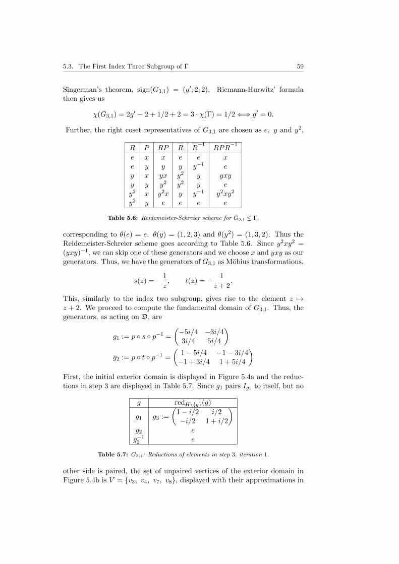
5.3. The First Index Three Subgroup of Γ 59
Singerman’s theorem, sign(G3,1) = (g′; 2; 2). Riemann-Hurwitz’ formulathen gives us
χ(G3,1) = 2g′ − 2 + 1/2 + 2 = 3 · χ(Γ) = 1/2⇐⇒ g′ = 0.
Further, the right coset representatives of G3,1 are chosen as e, y and y2,
R P RP R R−1
RPR−1
e x x e e xe y y y y−1 ey x yx y2 y yxyy y y2 y2 y ey2 x y2x y y−1 y2xy2
y2 y e e e e
Table 5.6: Reidemeister-Schreier scheme for G3,1 ≤ Γ.
corresponding to θ(e) = e, θ(y) = (1, 2, 3) and θ(y2) = (1, 3, 2). Thus theReidemeister-Schreier scheme goes according to Table 5.6. Since y2xy2 =(yxy)−1, we can skip one of these generators and we choose x and yxy as ourgenerators. Thus, we have the generators of G3,1 as Mobius transformations,
s(z) = −1
z, t(z) = − 1
z + 2.
This, similarly to the index two subgroup, gives rise to the element z 7→z + 2. We proceed to compute the fundamental domain of G3,1. Thus, thegenerators, as acting on D, are
g1 := p s p−1 =
(−5i/4 −3i/43i/4 5i/4
)g2 := p t p−1 =
(1− 5i/4 −1− 3i/4−1 + 3i/4 1 + 5i/4
)First, the initial exterior domain is displayed in Figure 5.4a and the reduc-tions in step 3 are displayed in Table 5.7. Since g1 pairs Ig1 to itself, but no
g redH\g(g)
g1 g3 :=
(1− i/2 i/2−i/2 1 + i/2
)g2 e
g−12 e
Table 5.7: G3,1: Reductions of elements in step 3, iteration 1.
other side is paired, the set of unpaired vertices of the exterior domain inFigure 5.4b is V = v3, v4, v7, v8, displayed with their approximations in

60 Chapter 5. Computations for Specific Fuchsian Groups
v vnumv3
18200(197 + 32
√24823 + i(6304−
√24823))
v41
8200(197− 32√
24823 + i(6304 +√
24823))
v71
1000(197− 2√
155191 + i(−394−√
155191))
v81
1000(197 + 2√
155191 + i(−394 +√
155191))
Table 5.8: G3,1: Unpaired vertices for iteration 1, step 5.
g v redH(g; vnum) δ
g2 v3 g4 :=
(−1 + 13i/4 3− 5i/4
3 + 5i/4 −1− 13i/4
) (−3− 3i/2 −2− 5i/2−2 + 5i/2 −3 + 3i/2
)g2 v4 g−1
3 :=
(−1− i/2 i/2−i/2 −1 + i/2
)g1
g3 v7 g3 eg3 v8 g3 e
Table 5.9: G3,1: Reductions on vertices in step 5.
Table 5.8. The reductions on the unpaired vertices are displayed in Table 5.9.Since this yields the side-pairing g1([v1, v2]) = [v2, v1], g3([v7, v8]) = [v10, v9]we are done. The final domain is displayed with normalised boundary inFigure 5.4c and with side-pairing in Figure 5.4d.
5.4 The Second Index Three Subgroup of Γ
Our second, and final, example of index three1 is the group, denoted G3,2,induced by the epimorphism
θ(x) = (1)(2)(3), θ(y) = (1, 2, 3) and θ(xy) = (1, 2, 3),
which yields the signature (0; 2, 2, 2; 1). The coset system for this group ischosen as e, y and y2. The Reidemeister-Schreier scheme is then displayedin Table 5.10, where in the last column we employ the relations of Γ. Thegenerators are then, as complex functions,
h1(z) = −1/z, h2(z) = − z + 1
2z + 1and h3(z) = −z + 2
z + 1
where h1 corresponds to x, h2 to yxy−1 and h3 to y−1xy.
Since x = x−1, another set of generators is
s1(z) = −1/z, s2(z) =z − 2
z − 1and s3(z) =
z + 1
z + 2,
1One more epimorphism satisfies the cycle conditions, but does not satisfy theRiemann-Hurwitz identity, instead yielding genus −1, which is clearly impossible.

5.4. The Second Index Three Subgroup of Γ 61
v1, v4
v2
v3
(a) The isometric circles ofg1, g2 and g−1
2 and their exteriordomain with normalised bound-ary.
v1, v4
v2, v7
v3
v8
(b) The isometric circles ofg1, g2, g−1
2 and g3 and theirexterior domain with normalisedboundary.
v1, v10
v2, v7
(c) The isometric circles ofg1, g2, g3, g
−13 and g4 and their
exterior domain with normalisedboundary.
v1, v10
v2, v7
v8, v9x1
(d) The isometric circles ofg1, g3, and g−1
3 with fundamen-tal domain and side-pairing.
Figure 5.4: Algorithmic computation for G3,1, all figures.
R P RP R R−1
RPR−1
e x x e e xe y y y y−1 ey x yx y y−1 yxy−1
y y y2 y2 (y2)−1 ey2 x y2x y2 (y2)−1 y−1xyy2 y y3 e e e
Table 5.10: Reidemeister-Schreier scheme for G3,2 ≤ Γ.

62 Chapter 5. Computations for Specific Fuchsian Groups
where s1 corresponds to x, s2 to xyxy−1x and s3 to xy−1xy. The conjugatedgenerators with inverses, H, are, then,
g1 = g−11 = ps−1
1 p−1 :=
(−5i/4 −3i/43i/4 5i/4
),
g2 = g−12 = ps2p
−1 :=
(−3i/2 1− i/21 + i/2 3i/2
),
g3 = ps3p−1 :=
(3/2− 3i/4 −1/2− 5i/4−1/2 + 5i/4 3/2 + 3i/4
), and
g−13 :=
(3/2 + 3i/4 1/2 + 5i/41/2− 5i/4 3/2− 3i/4
).
We use these generators for our computation, and their isometric circlesand normalised boundary U = (g3, g1, g2) are displayed in Figure 5.5a.The reductions of elements in H are then performed in Table 5.11, yield-ing the new element g4. This gives rise to the new normalised boundaryU = (g3, g1, g2, g4), displayed in Figure 5.5b. Then, the same reductionsare received and we proceed to the pairing of vertices, where g2 pairs theside [x2, x3] with [x3, x2]. The reductions on the unpaired vertices v5, x1 and
g redH\g(g)
g1 g1
g2 g4 :=
(1− 3i/4 3i/4−3i/4 1 + 3i/4
)g3 e
g−13 e
Table 5.11: G3,2: Reductions of elements in step 3, iteration 1.
v10 are shown in Table 5.12. As always, the ideal vertices v5 and v10 are ap-proximated as the intersection of their isometric circles with |z| =
√97/100.
g v redH(g; vnum)
g3 v5 g5 :=
(3− 3i −4− i−4 + i 3 + 3i
)g1 x1 g6 :=
(3/2 + 9i/4 5/2− i/45/2 + i/4 3/2− 9i/4
)g3 x1 g6
g4 v10 g4x
Table 5.12: G3,2: Reductions on vertices in step 5, iteration 1.
Thus, the new exterior domain, with the normalised boundary
U = (g5, g3, g6, g1, g2, g4)

5.4. The Second Index Three Subgroup of Γ 63
is shown in Figure 5.5c. In the reduction step in step 3 nothing new appears,so we move straight along to a new pairing check. Still, the only pairedvertices are x2 and x3, so we make reductions on the unpaired verticesv11, x4, x5, x6 and v10. They are shown in Table 5.13. The new exterior
g v redH(g; vnum)
g5 v11 g7 :=
(3 −2− 2i
−2 + 2i 3
)g5 x4 g8 :=
(−3/2 + 5i/4 3/2 + 3i/43/2− 3i/4 −3/2− 5i/4
)g3 x4 g8
g3 x5 g9 :=
(−3i/2 −1− i/2−1 + i/2 3i/2
)g6 x5 g6
g6 x6 g6
g1 x6 g3
g4 v10 g4
Table 5.13: G3,2: Reductions on vertices in step 5, iteration 2.
domain with normalised boundary U = (g7, g8, g3, g9, g1, g2, g4) is shownin Figure 5.5d.
There are no new reductions in step 3 and in the final step we find theside-pairings g1([x10, x2]) = [x2, x10], g2([x2, x3]) = [x3, x2] and g9([x9, x10]) =[x10, x9]. Thus, the reductions on unpaired vertices v15, x7, x8 and v10 aredisplayed in Table 5.14.
g v redH(g; vnum)
g7 v15 g10 :=
(−3/2− 23i/4 −9/2 + 15i/4−9/2− 15i/4 −3/2 + 23i/4
)g7 x7 g−1
4 :=
(−1− 3i/4 3i/4−3i/4 −1 + 3i/4
)g8 x7 g−1
4
g8 x8 g−14
g3 x8 g−14
g4 v10 g4
Table 5.14: G3,2: Reductions on vertices in step 5, iteration 3.
The new normalised boundary U = (g−14 , g9, g1, g2, g4), together with
the isometric circles, is displayed in Figure 5.5e. This is a side-pairing,according to
g1([x10, x2]) = [x2, x10], g2([x2, x3]) = [x3, x2],
g4([x3, v10]) = [x9, v21], g9([x9, x10]) = [x10, x9],

64 Chapter 5. Computations for Specific Fuchsian Groups
displayed in Figure 5.5f, with added mid-vertices for the elements of order2.
v4
v5
x1
x2
(a) The isometric circles ofg1, g2, g3 and g−1
3 and theirexterior domain with normalisedboundary.
v5
v10
x1
x2 x3
(b) The isometric circles ofg1, g2, g3, g
−13 and g4 and their
exterior domain with normalisedboundary.
v10
v11
x2 x3
x4x5
x6
(c) The isometric circles of g1,g2, g3, g4, g5 and g6 and theirexterior domain with normalisedboundary.
v10
v15
x2 x3
x7x8
x9
x10
(d) The isometric circles ofg1, g2, g3, g4, g5, g6, g7, g8 andg9 and their exterior domain withnormalised boundary.
x2 x3
x9
x10
(e) The isometric circles of g1,g2, g3, g4, g5, g6, g7, g8, g9, g10and g−1
4 and their exterior do-main with normalised boundary.
y1
y2
y3
x2 x3
x9
x10
v10, v21
(f) The isometric circles ofg1, g2, g4, g9 and g−1
4 and thefundamental domain with side-pairing.
Figure 5.5: Algorithmic computation for G3,2, all figures.
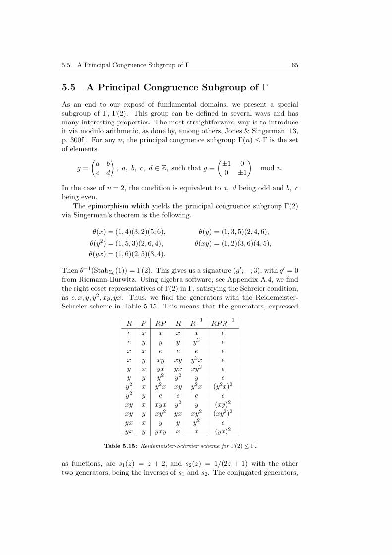
5.5. A Principal Congruence Subgroup of Γ 65
5.5 A Principal Congruence Subgroup of Γ
As an end to our expose of fundamental domains, we present a specialsubgroup of Γ, Γ(2). This group can be defined in several ways and hasmany interesting properties. The most straightforward way is to introduceit via modulo arithmetic, as done by, among others, Jones & Singerman [13,p. 300f]. For any n, the principal congruence subgroup Γ(n) ≤ Γ is the setof elements
g =
(a bc d
), a, b, c, d ∈ Z, such that g ≡
(±1 00 ±1
)mod n.
In the case of n = 2, the condition is equivalent to a, d being odd and b, cbeing even.
The epimorphism which yields the principal congruence subgroup Γ(2)via Singerman’s theorem is the following.
θ(x) = (1, 4)(3, 2)(5, 6), θ(y) = (1, 3, 5)(2, 4, 6),
θ(y2) = (1, 5, 3)(2, 6, 4), θ(xy) = (1, 2)(3, 6)(4, 5),
θ(yx) = (1, 6)(2, 5)(3, 4).
Then θ−1(StabΣ6(1)) = Γ(2). This gives us a signature (g′;−; 3), with g′ = 0from Riemann-Hurwitz. Using algebra software, see Appendix A.4, we findthe right coset representatives of Γ(2) in Γ, satisfying the Schreier condition,as e, x, y, y2, xy, yx. Thus, we find the generators with the Reidemeister-Schreier scheme in Table 5.15. This means that the generators, expressed
R P RP R R−1
RPR−1
e x x x x ee y y y y2 ex x e e e ex y xy xy y2x ey x yx yx xy2 ey y y2 y2 y ey2 x y2x xy y2x (y2x)2
y2 y e e e exy x xyx y2 y (xy)2
xy y xy2 yx xy2 (xy2)2
yx x y y y2 eyx y yxy x x (yx)2
Table 5.15: Reidemeister-Schreier scheme for Γ(2) ≤ Γ.
as functions, are s1(z) = z + 2, and s2(z) = 1/(2z + 1) with the othertwo generators, being the inverses of s1 and s2. The conjugated generators,

66 Chapter 5. Computations for Specific Fuchsian Groups
together with inverses, are then, in matrix form,
g1 =
(1 + i/2 −i/2i/2 1− i/2
), g2 =
(1− 2i −2i
2i 1 + 2i
),
g−11 =
(1− i/2 i/2−i/2 1 + i/2
), and g−1
2 =
(1 + 2i 2i−2i 1− 2i
).
The isometric circles together with normalised boundary are displayed inFigure 5.6a and since there are no reductions in step 3 and we have a side-pairing in step 5 as g1([v1, v2]) = [v4, v3] and g2([v5, v6]) = [v8, v7], with theirinverses in the opposite direction, all vertices are paired and the fundamentaldomain is displayed in Figure 5.6b.
Ig1
Ig−11
Ig2
Ig−12
v2, v5
v3, v8
v6, v7
(a) The isometric circles ofg1, g−1
1 , g2 and g−12 and their
exterior domain with normalisedboundary.
v1, v4
v2, v5
v3, v8
(b) The isometric circles ofg1, g−1
1 , g2 and g−12 and the
fundamental domain with side-pairing.
Figure 5.6: Algorithmic computation for Γ(2), all figures.
Chapter 6
Discussion
We have given an exposition of some methods to help in the study of theimportant and interesting area of fundamental polygons. The combinatorialmethods of Singerman and Reidemeister-Schreier can thus be used to givea starting point for the algorithmic computation of Dirichlet/Ford domainsfrom the generators of the group. This provides a unified way to go fromcertain cofinite Fuchsian groups to get the Dirichlet/Ford domain for itssubgroups of a given index. Since we already get a new domain from theimplicit conditions of Singerman’s theorem, a legitimate question is what isthe real gain to be had from such an extensive approach. First of all, thereis the question of explicit generators, which we get from the Reidemeister-Schreier method, and secondly we do not know what type of domain weget from the implicit conditions. It is certainly not necessary that it is aDirichlet domain, whereas the transfer to a Dirichlet domain is guaranteedby this method in the case of cofinite groups. Moreover, the algorithmicapproach opens up the possibility of automation and can thus aid in raisingnew types of questions that can be asked by allowing a faster constructionof fundamental domains and making the process less ad hoc.
Some things have been glossed over, in order not to burden the exposi-tion, but as an elucidation of the previous paragraph we make some remarks.For instance, we have not touched upon the fundamental group, even thoughits connection to the side-pairing of a polygon is intimate. A brief introduc-tion is due. To start with, path homotopy is the continuous transformationof two curves with the same end-points into each other while keeping theend-points fixed. Moreover, we are able to invert, by taking the curve inopposite direction, and adjoin curves, by letting one curve γ : [0, 1]→ X beimmediately followed by another curve δ : [0, 1]→ X with γ(1) = δ(0). Thefundamental group is based at a regular point (not a branch-point) of thespace, x0. Curves both starting and ending at x0 can either be transformedinto each other by path homotopy or not. This divides the set of all curvesinto equivalence classes, which under adjoining and inverse acts as a group,
Larsson, 2015. 67

68 Chapter 6. Discussion
known as the fundamental group. See [15, Chapter 9].Moreover, due to the branched covering, we are in reality working with
something called orbifolds and orbifold coverings, which are a generalisationof the concept of manifold, by making the neighbourhood of each pointhomeomorphic to a quotient of a neighbourhood of Rn. Topologically, theyare the same, but orbifolds do not have a geometric structure in precisely thesame sense as manifolds, due to the existence of branch-points. Outside thesepoints an orbifold acts as a manifold. Recall in this context Figure 2.3b,which is really a quotient map p : D → D/Z3, whereas regular points havea trivial quotient group. See [19, p. 185f]. Moreover, the orbifold has as itsfundamental group, in an isomorphic sense, the Fuchsian group, which hasnow been made explicit in terms of its generators and the side-pairing ofthe Dirichlet domain. Thus, we get the entire geometry of the orbifold fromthe fundamental polygon, together with a presentation for its fundamentalgroup: the Fuchsian group.
6.1 Suggestions for Further Study
A number of areas have opened themselves up for further study. There isperhaps a possibility to loosen some of the requirements of Voight’s algo-rithm in Section 4.3, so that reduction need not be done on the isometriccircle, but perhaps only outside the exterior domain. Moreover, it would beinteresting to think about the problem of hyperbolic boundary elements inthis regard, since the algorithm at this point only works for cofinite groups.
In terms of implementation of the algorithm, there is currently somethought going into some form of visualisation software to take advantageof the methods presented and make them more accessible to larger parts ofthe community. This could, for instance, be used to look for patterns inthe fundamental domains of subgroups of the modular group or to see whathappens when the centre of the Dirichlet domain is shifted.
Some other directions of investigation would be discrete subgroups ofPSL(2,C). As the reader will recall from Section 4.1, the Ford domain isnot limited to Fuchsian groups, but can be used for such Kleinian groups aswell.
Another direction, where there has been some progress in later years, dueto Paul Watson and David Singerman, is in the area of NEC groups, whichare discrete groups of isometries, i.e., generalisations of Fuchsian groups,allowing orientation-reversing elements. This is still unpublished research,but a pre-print can be found in [18].
Finally, in 2013, Jane Gilman presented an outline of an algorithm toeliminate generators and relations to give a better homological basis for con-formal automorphism groups of Riemann surfaces using the Reidemeister-Schreier method. See [11, p. 137-153].

Appendix A
Code Transcripts
In the appendix, we display transcripts of C++ functions and GAP computa-tions.
A.1 Common C++ Functions
Displayed below are the C++ functions that were used by both functions.Common was also the usage of the symbolic computation library GiNaC.
#include <iostream>
#include "ginac/ginac.h"
using namespace std;
using namespace GiNaC;
matrix twoInv(matrix M)
matrix MInv(2,2);
MInv = M(1,1),-M(0,1),-M(1,0),M(0,0);
MInv = MInv.mul_scalar(1/M.determinant());
return MInv;
const symbol z("z");
const numeric p = 2*I;
const matrix UH2D(2,2,lst(1,-p,1,-conjugate(p)));
const matrix D2UH = twoInv(UH2D);
numeric conjugate(numeric x)
return real(x) - I*imag(x);
Larsson, 2015. 69

70 Appendix A. Code Transcripts
numeric phypdist(numeric z1, numeric z2)
return
log((abs(z1-conjugate(z2))+abs(z1-z2))/
(abs(z1-conjugate(z2))-abs(z1-z2)));
// Calculate the hyperbolic distance between z1
// and z2 in the unit disc model.
numeric dhypdist(numeric z1, numeric z2)
numeric hz1 = (conjugate(p)*z1-p)/(z1-1);
numeric hz2 = (conjugate(p)*z2-p)/(z2-1);
return phypdist(hz1,hz2);
ex matToFn(matrix M)
return (M(0,0)*z+M(0,1))/(M(1,0)*z+M(1,1));
numeric redmap(const matrix& m, const numeric& n)
ex f = matToFn(m).subs(z == n);
if (is_a<numeric>(f))
return dhypdist(ex_to<numeric>(f),numeric(0));
else
cerr << "redmap: evaluation failed!" << endl;
matrix compose(const matrix& m1, const matrix& m2)
return m1.mul(m2);
numeric applyMat(const matrix& m, const numeric& n)
return ex_to<numeric>(matToFn(m).subs(z==n));
matrix plane2discmatrix(const matrix& m)

A.2. Computing the Reduction Map in C++ 71
return compose(UH2D,compose(m,D2UH));
matrix disc2planematrix(const matrix& m)
return compose(D2UH,compose(m,UH2D));
A.2 Computing the Reduction Map in C++
The following displays the code used to implement Algorithm 4.3, with ex-ample values for the incoming elements and reduction point.
int main()
matrix reduceThisMatrix(2,2);
numeric reduceWRTPoint(.52-.84*I); // The reduction point.
vector<pair<matrix,numeric>> setElements;
matrix setMatrix1(2,2);
matrix setMatrix1i(2,2);
matrix setMatrix2(2,2);
matrix setMatrix2i(2,2);
setMatrix1 = plane2discmatrix(matrix(2,2,lst(0,-1,1,1)));
setMatrix1i = twoInv(setMatrix1);
setMatrix2 = plane2discmatrix(matrix(2,2,lst(1,-1,1,0)));
setMatrix2i = twoInv(setMatrix2);
reduceThisMatrix = setMatrix1;
cout << "gamma = " << reduceThisMatrix << endl;
setElements.push_back(pair<matrix,numeric>(setMatrix2,0));
setElements.push_back(pair<matrix,numeric>(setMatrix1i,0));
setElements.push_back(pair<matrix,numeric>(setMatrix2i,0));
matrix reducedMatrix(2,2);
reducedMatrix = reduceThisMatrix;
matrix reductionMatrix(2,2);
reductionMatrix = 1,0,0,1;
numeric r, r_iMin;
matrix g(2,2);
do
r = redmap(reducedMatrix,reduceWRTPoint);
cout << "r = " << r << endl;
r_iMin = pow(numeric(10),numeric(60));
for (auto it : setElements)
it.second = redmap(compose(it.first,reducedMatrix),
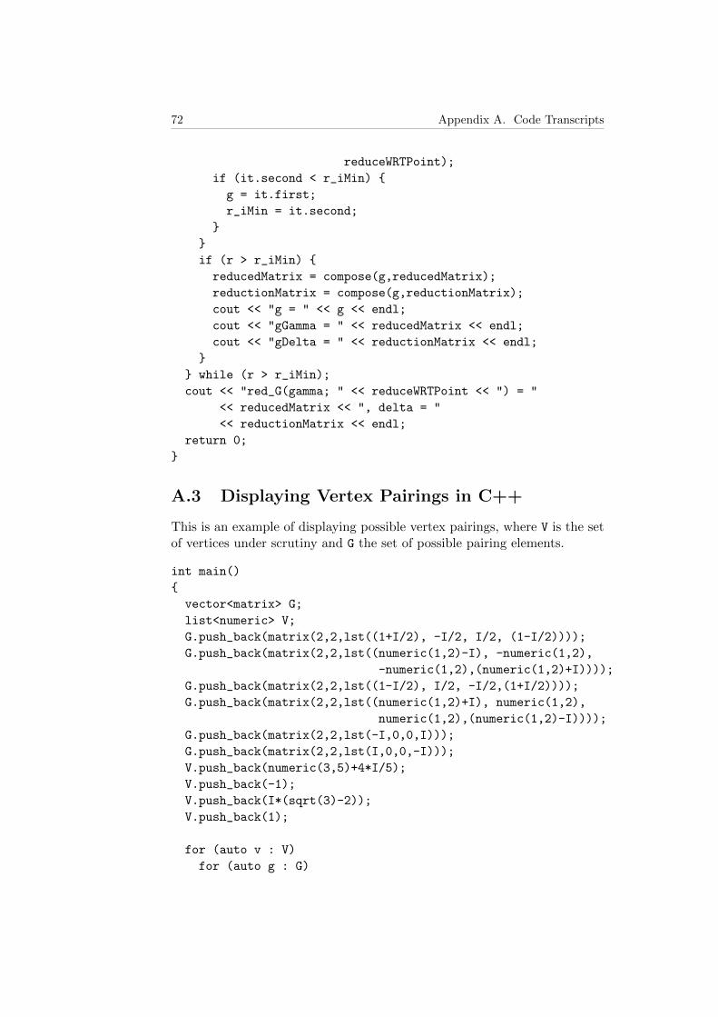
72 Appendix A. Code Transcripts
reduceWRTPoint);
if (it.second < r_iMin)
g = it.first;
r_iMin = it.second;
if (r > r_iMin)
reducedMatrix = compose(g,reducedMatrix);
reductionMatrix = compose(g,reductionMatrix);
cout << "g = " << g << endl;
cout << "gGamma = " << reducedMatrix << endl;
cout << "gDelta = " << reductionMatrix << endl;
while (r > r_iMin);
cout << "red_G(gamma; " << reduceWRTPoint << ") = "
<< reducedMatrix << ", delta = "
<< reductionMatrix << endl;
return 0;
A.3 Displaying Vertex Pairings in C++
This is an example of displaying possible vertex pairings, where V is the setof vertices under scrutiny and G the set of possible pairing elements.
int main()
vector<matrix> G;
list<numeric> V;
G.push_back(matrix(2,2,lst((1+I/2), -I/2, I/2, (1-I/2))));
G.push_back(matrix(2,2,lst((numeric(1,2)-I), -numeric(1,2),
-numeric(1,2),(numeric(1,2)+I))));
G.push_back(matrix(2,2,lst((1-I/2), I/2, -I/2,(1+I/2))));
G.push_back(matrix(2,2,lst((numeric(1,2)+I), numeric(1,2),
numeric(1,2),(numeric(1,2)-I))));
G.push_back(matrix(2,2,lst(-I,0,0,I)));
G.push_back(matrix(2,2,lst(I,0,0,-I)));
V.push_back(numeric(3,5)+4*I/5);
V.push_back(-1);
V.push_back(I*(sqrt(3)-2));
V.push_back(1);
for (auto v : V)
for (auto g : G)

A.4. Computing Right Cosets in GAP 73
cout << "v : " << v << "\t g : " << g << "\t g(v) : "
<< ex_to<numeric>(matToFn(g).subs(z == v)) << endl;
return 0;
A.4 Computing Right Cosets in GAP
The output from GAP, see [6], when computing the Schreier representativesof the right cosets of H := StabΣ6(1) in Σ6. We know that (1, n) givesdifferent cosets for n = 2, 3, 4, 5, 6, and find appropriate coset representativesby finding in which coset the images of the words x, y and so on are.
gap> G := Group((1,2),(1,3),(1,4),(1,5),(1,6),(2,3),(2,4),(2,5),
(2,6),(3,4),(3,5),(3,6),(4,5),(4,6),(5,6));
Group([ (1,2), (1,3), (1,4), (1,5), (1,6), (2,3), (2,4), (2,5),
(2,6), (3,4), (3,5), (3,6), (4,5), (4,6), (5,6) ])
gap> H := Stabilizer(G,1);
Group([ (2,3), (2,4), (2,5), (2,6), (3,4), (3,5), (3,6), (4,5),
(4,6), (5,6) ])
gap> one := RightCoset(H,());
RightCoset(Group( [ (2,3), (2,4), (2,5), (2,6), (3,4), (3,5),
(3,6), (4,5), (4,6), (5,6) ] ),())
gap> two := RightCoset(H,(1,2));
RightCoset(Group( [ (2,3), (2,4), (2,5), (2,6), (3,4), (3,5),
(3,6), (4,5), (4,6), (5,6) ] ),(1,2))
gap> three := RightCoset(H,(1,3));
RightCoset(Group( [ (2,3), (2,4), (2,5), (2,6), (3,4), (3,5),
(3,6), (4,5), (4,6), (5,6) ] ),(1,3))
gap> four := RightCoset(H,(1,4));
RightCoset(Group( [ (2,3), (2,4), (2,5), (2,6), (3,4), (3,5),
(3,6), (4,5), (4,6), (5,6) ] ),(1,4))
gap> five := RightCoset(H,(1,5));
RightCoset(Group( [ (2,3), (2,4), (2,5), (2,6), (3,4), (3,5),
(3,6), (4,5), (4,6), (5,6) ] ),(1,5))
gap> six := RightCoset(H,(1,6));
RightCoset(Group( [ (2,3), (2,4), (2,5), (2,6), (3,4), (3,5),
(3,6), (4,5), (4,6), (5,6) ] ),(1,6))
gap> (1,4)(3,2)(5,6) in one;
false
gap> (1,4)(3,2)(5,6) in two;
false
gap> (1,4)(3,2)(5,6) in three;
false
gap> (1,4)(3,2)(5,6) in four;

74 Appendix A. Code Transcripts
true
gap> (1,3,5)(2,4,6) in one;
false
gap> (1,3,5)(2,4,6) in two;
false
gap> (1,3,5)(2,4,6) in three;
true
gap> (1,5,3)(2,6,4) in one;
false
gap> (1,5,3)(2,6,4) in two;
false
gap> (1,5,3)(2,6,4) in three;
false
gap> (1,5,3)(2,6,4) in four;
false
gap> (1,5,3)(2,6,4) in five;
true
gap> (1,2)(3,6)(4,5) in one;
false
gap> (1,2)(3,6)(4,5) in two;
true
gap> (1,6)(2,5)(3,4) in one;
false
gap> (1,6)(2,5)(3,4) in two;
false
gap> (1,6)(2,5)(3,4) in three;
false
gap> (1,6)(2,5)(3,4) in four;
false
gap> (1,6)(2,5)(3,4) in five;
false
gap> (1,6)(2,5)(3,4) in six;
true
Thus, a set of coset representatives of H, that in the pre-image satisfiesSchreier’s condition, are θ(e) for the stabiliser itself, θ(x) for H · (1, 4), θ(y)for H · (1, 3), θ(y2) for H · (1, 5), θ(xy) for H · (1, 2) and θ(yx) for H · (1, 6).This means that e, x, y, y2, xy, yx are representatives of the cosets of Γ(2) inΓ.
Remark A.1. The reason we test through from the beginning is to see ifwe have arrived at the same coset by some previous element of Σ6 or if theelement is in fact in the stabiliser subgroup.

Bibliography
[1] G. Bartolini. On the Branch Loci of Moduli Spaces of Riemann Surfaces.Ph.D. Thesis, Linkopings Universitet, 2012.
[2] A. F. Beardon. The Geometry of Discrete Groups. Springer-Verlag,New York, 1995.
[3] C. B. Boyer. A History of Mathematics. Princeton University Press,Princeton, 1985.
[4] H. S. Coxeter and W. O. J. Moser. Generators and Relations for Dis-crete Groups. Springer-Verlag, Berlin, 1984.
[5] L. R. Ford. Automorphic Functions. Chelsea Publishing Company, NewYork, 1951.
[6] GAP. http://www.gap-system.org. Last fetched 2015-06-02.
[7] GiNaC is not a CAS. http://www.ginac.de. Last fetched 2015-06-02.
[8] P. A. Grillet. Abstract Algebra, 2nd Edition. Springer-Verlag, NewYork, 2007.
[9] Y. Grosman and W. Magnus. Groups and their graphs. Anneli LaxNew Mathematical Library: 14. Mathematical Association of America,Washington D.C., 1992.
[10] A. Hurwitz. Ueber Riemann’sche Flachen mit gegebenen Verzwei-gungspunkten. Mathematische Annalen, 39(1):1–60, 1891.
[11] M. Izquierdo, S. A. Broughton, A. F. Costa, and R. E. Rodrıguez.Riemann and Klein Surfaces, Automorphisms, Symmetries and ModuliSpaces (Contemporary Mathematics). American Mathematical Society,2014.
[12] M. Izquierdo and D. Ying. Equisymmetric strata of the moduli spaceof cyclic trigonal Riemann surfaces of genus 4. Glasgow MathematicalJournal, 51(1):19–29, 2009.
Larsson, 2015. 75
76 Bibliography
[13] G. A. Jones and D. Singerman. Complex Functions: An Algebraic andGeometric Viewpoint. Cambridge University Press, Cambridge, 1987.
[14] W. S. Massey. Algebraic Topology: An Introduction. Springer-Verlag,New York, 1990.
[15] J. R. Munkres. Topology. Pearson New International Edition. PearsonEducation Limited, Harlow, 2013.
[16] H. Poincare. The Foundations of Science: Science and Hypothe-sis, The Value of Science, Science and Method. Project Guten-berg, http://www.gutenberg.org/files/39713/39713-h/39713-h.
htm, 2012. Translated by G.B. Halsted.
[17] D. Singerman. Subgroups of Fuchsian groups and finite permutationgroups. Bulletin of the London Mathematical Society, 2(3):319–323,1970.
[18] D. Singerman and P. Watson. Using Hoare’s Theorem to find the signa-ture of a subgroup of an NEC group. Pre-print, 2014. arXiv:1408.0127[math.GR].
[19] J. Stillwell. Geometry of Surfaces. Springer-Verlag, New York, 1995.
[20] J. Voight. Computing fundamental domains for Fuchsian groups. J.Theor. Nombres Bordeaux, 21(2):469–491, 2009.
[21] Wolfram|Alpha. http://www.wolframalpha.com. Last fetched 2015-06-02.
[22] H. Zieschang, E. Vogt, and H.-D. Coldewey. Surfaces and Planar Dis-continuous Groups. Springer-Verlag, Berlin, 1980.

Copyright
The publishers will keep this document online on the Internet - or itspossible replacement - for a period of 25 years from the date of publica-tion barring exceptional circumstances. The online availability of the doc-ument implies a permanent permission for anyone to read, to download, toprint out single copies for your own use and to use it unchanged for anynon-commercial research and educational purpose. Subsequent transfers ofcopyright cannot revoke this permission. All other uses of the documentare conditional on the consent of the copyright owner. The publisher hastaken technical and administrative measures to assure authenticity, securityand accessibility. According to intellectual property law the author has theright to be mentioned when his/her work is accessed as described above andto be protected against infringement. For additional information about theLinkoping University Electronic Press and its procedures for publication andfor assurance of document integrity, please refer to its WWW home page:http://www.ep.liu.se/
Upphovsratt
Detta dokument halls tillgangligt pa Internet - eller dess framtida ersattare- under 25 ar fran publiceringsdatum under forutsattning att inga extraordi-nara omstandigheter uppstar. Tillgang till dokumentet innebar tillstand forvar och en att lasa, ladda ner, skriva ut enstaka kopior for enskilt brukoch att anvanda det oforandrat for ickekommersiell forskning och for un-dervisning. Overforing av upphovsratten vid en senare tidpunkt kan inteupphava detta tillstand. All annan anvandning av dokumentet kraver up-phovsmannens medgivande. For att garantera aktheten, sakerheten ochtillgangligheten finns det losningar av teknisk och administrativ art. Up-phovsmannens ideella ratt innefattar ratt att bli namnd som upphovsman iden omfattning som god sed kraver vid anvandning av dokumentet pa ovanbeskrivna satt samt skydd mot att dokumentet andras eller presenteras isadan form eller i sadant sammanhang som ar krankande for upphovsman-nens litterara eller konstnarliga anseende eller egenart. For ytterligare in-formation om Linkoping University Electronic Press se forlagets hemsidahttp://www.ep.liu.se/
c© 2015, David Larsson
Larsson, 2015. 77