Estimation of Reverberation Time from Binaural...
30
Estimation of Reverberation Time from Binaural Signals Without Using Controlled Excitation Sampo Vesa Master’s Thesis presentation on 22nd of September, 2004 21st September 2004 HUT / Laboratory of Acoustics and Audio Signal Processing Page 1
-
Upload
truongnguyet -
Category
Documents
-
view
220 -
download
0
Transcript of Estimation of Reverberation Time from Binaural...

Estimation of Reverberation Time from
Binaural Signals Without Using Controlled
Excitation
Sampo VesaMaster’s Thesis presentation on 22nd of September, 2004
21st September 2004 HUT / Laboratory of Acoustics and Audio Signal Processing Page 1

Outline
Background
The problem
The algorithm
Evaluation results
Future work and conclusions
21st September 2004 HUT / Laboratory of Acoustics and Audio Signal Processing Page 2

Background
Motivation and goals of the work
• An RT estimate would be beneficial in many applications
• It is not feasible to feed a measurement signal into the environment
• Passively received binaural signal is available in some applications
• The goal of this work was to develop a reverberation time estimation
method that takes advantage of the binaural nature of the signals
21st September 2004 HUT / Laboratory of Acoustics and Audio Signal Processing Page 3
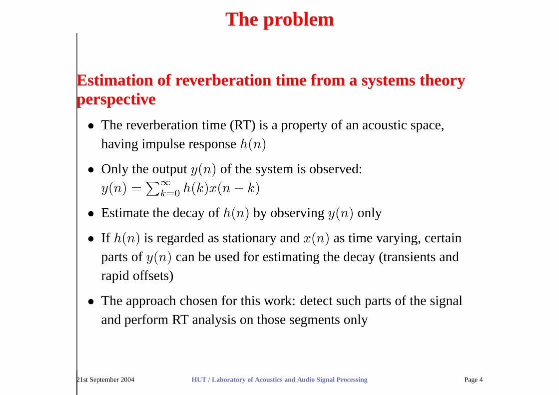
The problem
Estimation of reverberation time from a systems theoryperspective
• The reverberation time (RT) is a property of an acoustic space,having impulse response h(n)
• Only the output y(n) of the system is observed:y(n) =
∑∞
k=0h(k)x(n − k)
• Estimate the decay of h(n) by observing y(n) only
• If h(n) is regarded as stationary and x(n) as time varying, certainparts of y(n) can be used for estimating the decay (transients andrapid offsets)
• The approach chosen for this work: detect such parts of the signaland perform RT analysis on those segments only
21st September 2004 HUT / Laboratory of Acoustics and Audio Signal Processing Page 4
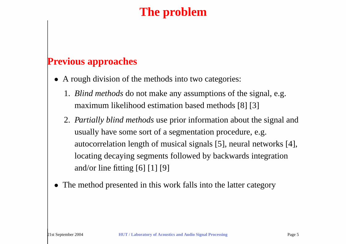
The problem
Previous approaches
• A rough division of the methods into two categories:
1. Blind methods do not make any assumptions of the signal, e.g.
maximum likelihood estimation based methods [8] [3]
2. Partially blind methods use prior information about the signal and
usually have some sort of a segmentation procedure, e.g.
autocorrelation length of musical signals [5], neural networks [4],
locating decaying segments followed by backwards integration
and/or line fitting [6] [1] [9]
• The method presented in this work falls into the latter category
21st September 2004 HUT / Laboratory of Acoustics and Audio Signal Processing Page 5

The algorithm
Structure of the proposed algorithm
1. Segmentation
2. Locating the limits of Schroeder integration
3. Testing the segments
4. Backwards integration (if segment was accepted)
5. LS fit with fixed or variable range → RT estimate
6. Statistical analysis on all RT values up to this point → final RT
estimate
21st September 2004 HUT / Laboratory of Acoustics and Audio Signal Processing Page 6
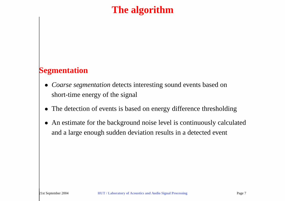
The algorithm
Segmentation
• Coarse segmentation detects interesting sound events based on
short-time energy of the signal
• The detection of events is based on energy difference thresholding
• An estimate for the background noise level is continuously calculated
and a large enough sudden deviation results in a detected event
21st September 2004 HUT / Laboratory of Acoustics and Audio Signal Processing Page 7

The algorithm
Finding the limits of Schroeder integration
• A practical formula for applying the Schroeder method is [2]:
D(t) = N
∫Ti
t
h2(τ)dτ (1)
• Fine segmentation attempts to find optimal Schroeder integration
limits:
– Ti is the upper limit of integration in Eq. 1
– Td is the point up to which the decay curve is evaluated
21st September 2004 HUT / Laboratory of Acoustics and Audio Signal Processing Page 8

The algorithm
−80
−60
−40
−20
0
Ene
rgy
/ dB
0 0.5 1 1.5 2 2.5 3
x 104
0
0.2
0.4
0.6
0.8
1
Sample index
Ave
rage
coh
eren
ce
Td Ti
Figure 1: An example of Schroeder integration with the limits Ti and Td
21st September 2004 HUT / Laboratory of Acoustics and Audio Signal Processing Page 9

The algorithm
Finding Ti, the upper limit of Schroeder integration
• Ti should ideally be at the point where the decay “dives” into the
noise floor
• A special algorithm for locating Ti is reported in [7]
• This work uses a simpler approach based on calculating a probability
density function estimate from an energy envelope of the segment
• Details can be found from the thesis
21st September 2004 HUT / Laboratory of Acoustics and Audio Signal Processing Page 10

The algorithm
Finding Td, the point up to which the decay curve isevaluated
• Td should ideally be at the point where the diffuse decay starts
• The short-time average interaural coherence (STAIC) has beenpreviously used for measuring the diffusiveness of an acousticalsituation [10]
• The STAIC is evaluated from short-time Fourier transforms
• Calculate the length of the part of the segment that has STAIC valuesover a certain threshold (e.g. 0.8) and sum with the location of themaximum of the envelope
• Always more or less overestimated this way (does not matter)
• A simpler alternative: locate the -5 dB point on the envelope
21st September 2004 HUT / Laboratory of Acoustics and Audio Signal Processing Page 11
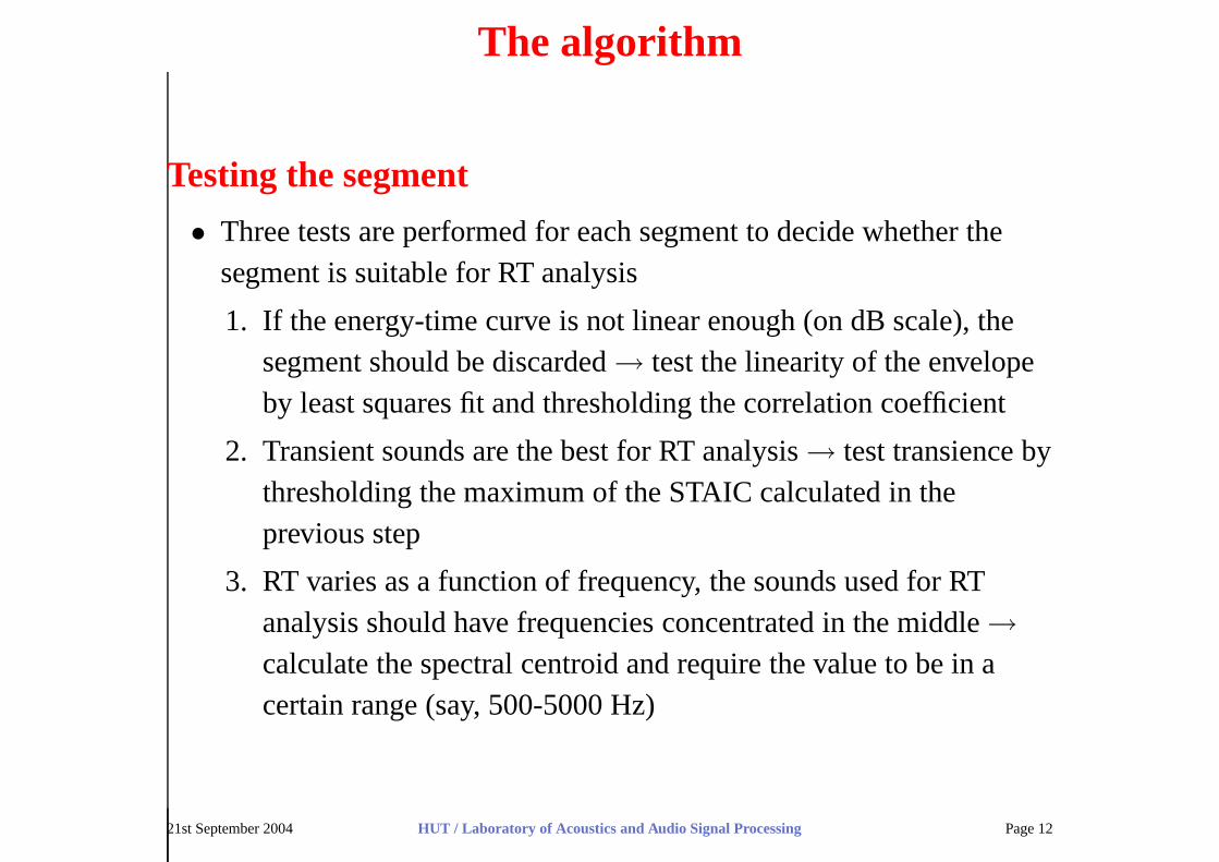
The algorithm
Testing the segment
• Three tests are performed for each segment to decide whether thesegment is suitable for RT analysis
1. If the energy-time curve is not linear enough (on dB scale), thesegment should be discarded → test the linearity of the envelopeby least squares fit and thresholding the correlation coefficient
2. Transient sounds are the best for RT analysis → test transience bythresholding the maximum of the STAIC calculated in theprevious step
3. RT varies as a function of frequency, the sounds used for RTanalysis should have frequencies concentrated in the middle →
calculate the spectral centroid and require the value to be in acertain range (say, 500-5000 Hz)
21st September 2004 HUT / Laboratory of Acoustics and Audio Signal Processing Page 12

The algorithm
Backwards integration (the Schroeder method)
• If the segment passed all three tests, the decay curve is calculated for
range [Ti, Td] by using discretized version of the Schroeder method
• Eq. 1 is the basis of this section of the algorithm
21st September 2004 HUT / Laboratory of Acoustics and Audio Signal Processing Page 13

The algorithm
Line fitting with fixed or variable limits
• Least squares method is used to fit a line to the decay curve
• RT easily derived from the slope of the line
• Normally the line is fit to a range of -5 to -35 dB (T30) or -5 to -25 dB
(T20)
• The signal-to-noise ratio (SNR) does not always permit this
• Solution: fit the line to a range that maximizes the correlation
coefficient
• Removes the possible systematic bias caused by bending of the decay
curves!
21st September 2004 HUT / Laboratory of Acoustics and Audio Signal Processing Page 14

The algorithm
Perform statistical analysis
• Finally, statistical analysis is performed on all estimates including the
current one
• Possible statistics to use: mean, median, order statistics, peak of
histogram...
• The first peak of the histogram sounds good for this application
• Three different statistics (mean, median and histogram peak) were
compared in the evaluation part of the thesis
21st September 2004 HUT / Laboratory of Acoustics and Audio Signal Processing Page 15
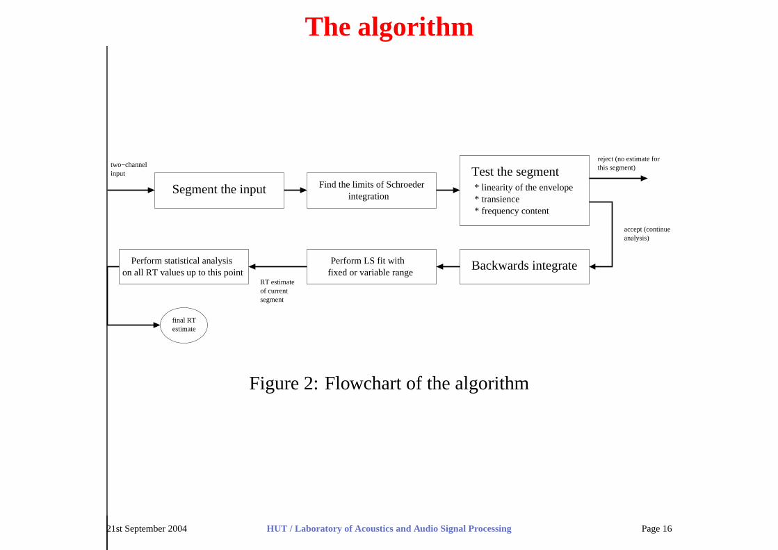
The algorithm
RT estimateof currentsegment
final RTestimate
fixed or variable range
* linearity of the envelope* transience* frequency content
integration
inputtwo−channel
reject (no estimate forthis segment)
accept (continueanalysis)
Find the limits of SchroederTest the segment
Perform LS fit with Backwards integrate
Segment the input
on all RT values up to this pointPerform statistical analysis
Figure 2: Flowchart of the algorithm
21st September 2004 HUT / Laboratory of Acoustics and Audio Signal Processing Page 16
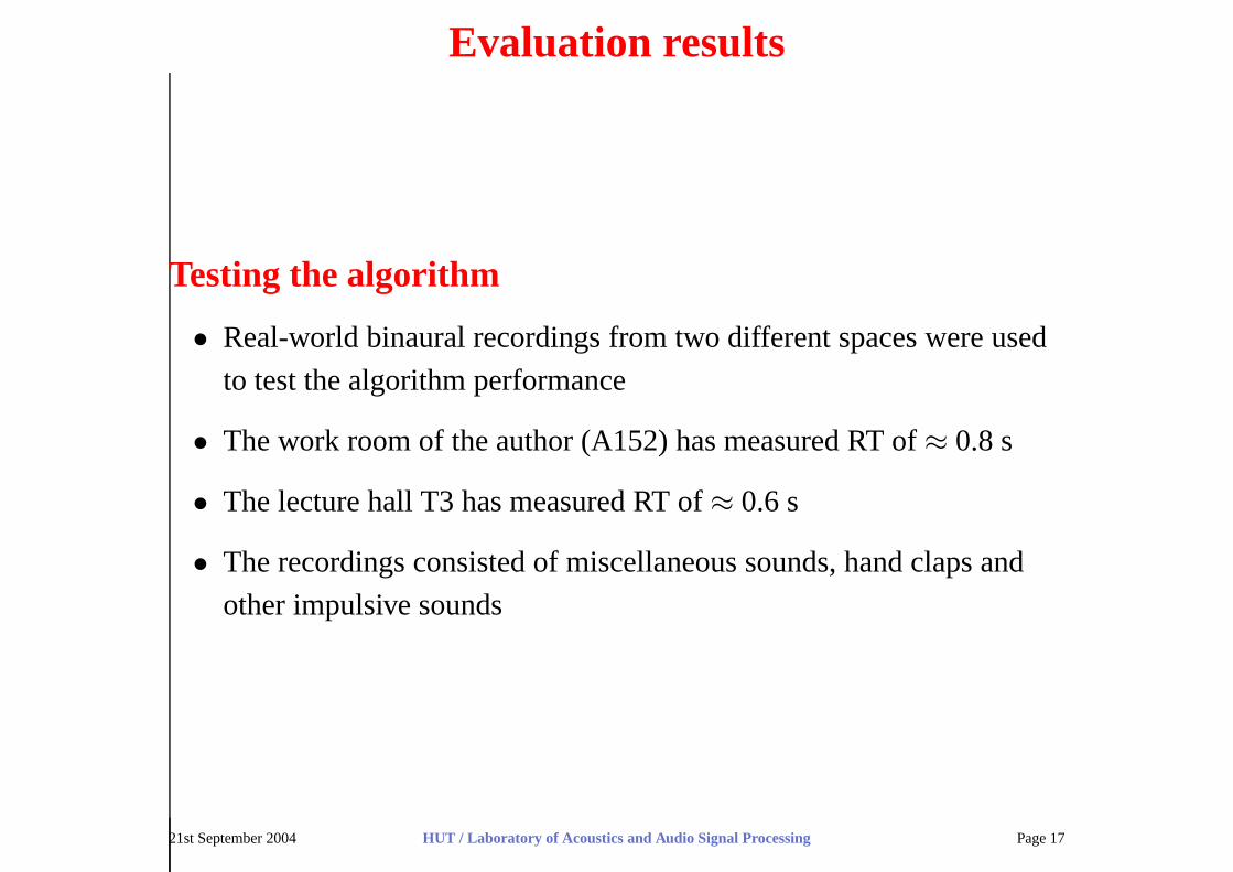
Evaluation results
Testing the algorithm
• Real-world binaural recordings from two different spaces were used
to test the algorithm performance
• The work room of the author (A152) has measured RT of ≈ 0.8 s
• The lecture hall T3 has measured RT of ≈ 0.6 s
• The recordings consisted of miscellaneous sounds, hand claps and
other impulsive sounds
21st September 2004 HUT / Laboratory of Acoustics and Audio Signal Processing Page 17

Evaluation results
21st September 2004 HUT / Laboratory of Acoustics and Audio Signal Processing Page 18

Evaluation results
10 20 300
0.2
0.4
0.6
0.8
1
1.2
1.4
1.6
1.8
2
RT
/ s
Index
T60
, LS fit to −5 to −25 dB
true value
10 20 300
0.2
0.4
0.6
0.8
1
1.2
1.4
1.6
1.8
2
RT
/ s
Index
T60
, LS fit with algorithm
true value
Figure 3: Estimates of T60 for room A152 with and without least squares
limit lookup, real recording
21st September 2004 HUT / Laboratory of Acoustics and Audio Signal Processing Page 19

Evaluation results
0
0.5
1
1.5
2
RT
/ s
meantrue value
0
0.5
1
1.5
2R
T /
smediantrue value
5 10 15 20 25 30 350
0.5
1
1.5
2
RT
/ s
Index
peak value of hist.true value
Figure 4: Three different statistics calculated from T60 estimates for room
A152, real recording, line fitting range -5 to -25 dB
21st September 2004 HUT / Laboratory of Acoustics and Audio Signal Processing Page 20

Evaluation results
0
0.5
1
1.5
2
RT
/ s
meantrue value
0
0.5
1
1.5
2R
T /
smediantrue value
5 10 15 20 25 30 350
0.5
1
1.5
2
RT
/ s
Index
peak value of hist.true value
Figure 5: Three different statistics calculated from T60 estimates for room
A152, real recording, variable line fitting limits
21st September 2004 HUT / Laboratory of Acoustics and Audio Signal Processing Page 21
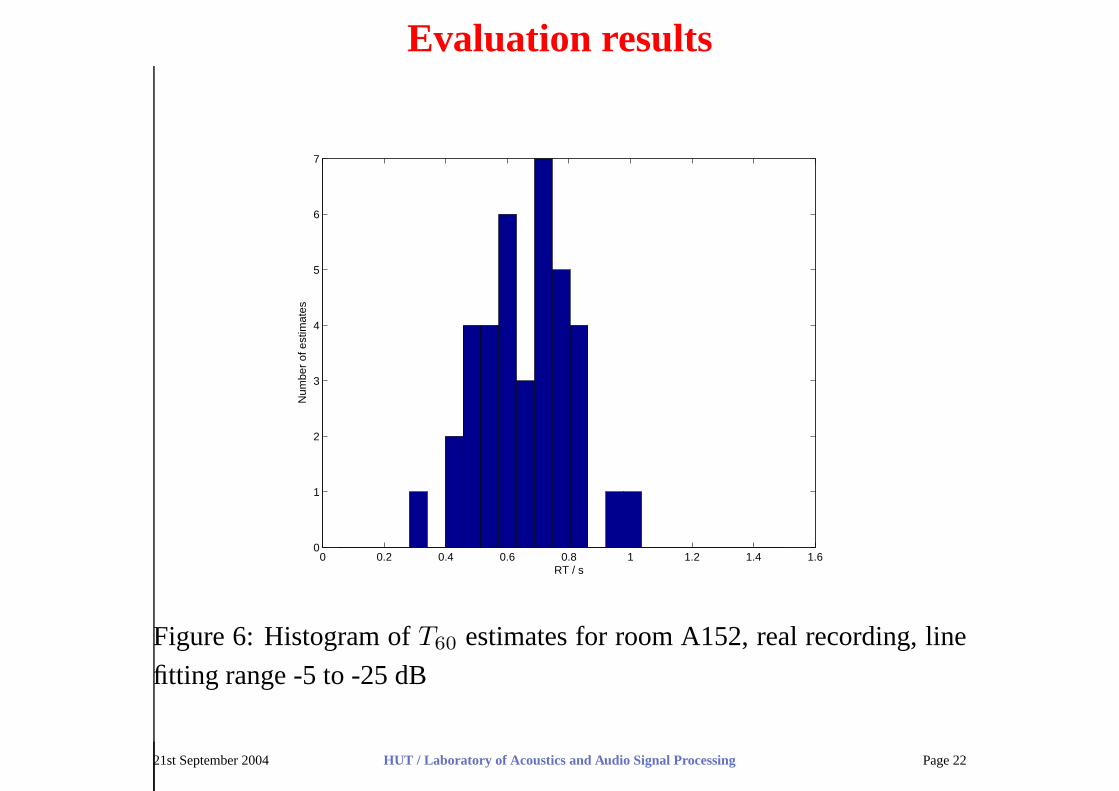
Evaluation results
0 0.2 0.4 0.6 0.8 1 1.2 1.4 1.60
1
2
3
4
5
6
7
Num
ber
of e
stim
ates
RT / s
Figure 6: Histogram of T60 estimates for room A152, real recording, line
fitting range -5 to -25 dB
21st September 2004 HUT / Laboratory of Acoustics and Audio Signal Processing Page 22

Evaluation results
0 0.2 0.4 0.6 0.8 1 1.2 1.4 1.60
0.5
1
1.5
2
2.5
3
3.5
4
4.5
5
Num
ber
of e
stim
ates
RT / s
Figure 7: Histogram of T60 estimates for room A152, real recording, vari-
able line fitting limits
21st September 2004 HUT / Laboratory of Acoustics and Audio Signal Processing Page 23

Evaluation results
0
0.5
1
1.5
2
RT
/ s
meantrue value
0
0.5
1
1.5
2R
T /
s
mediantrue value
5 10 15 20 25 30 35 40 45 50 550
0.5
1
1.5
2
RT
/ s
Index
peak value of hist.true value
Figure 8: Three different statistics calculated from T60 estimates for room
T3, real recording, variable line fitting limits
21st September 2004 HUT / Laboratory of Acoustics and Audio Signal Processing Page 24
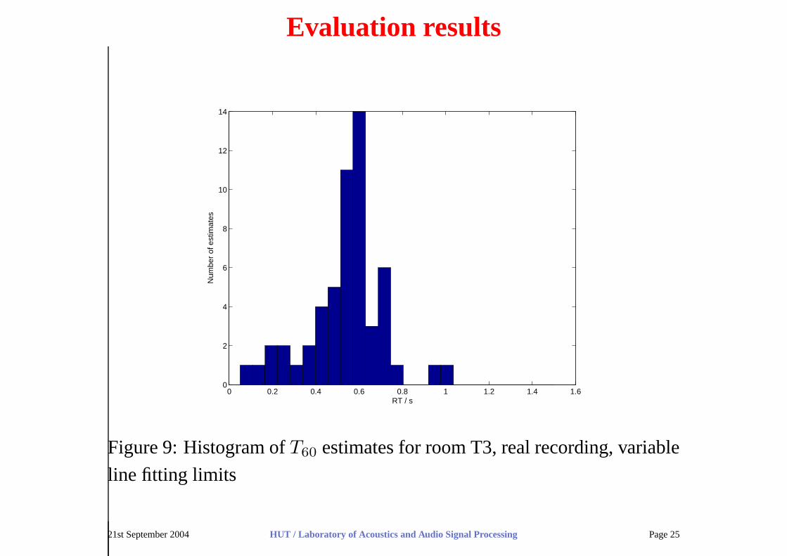
Evaluation results
0 0.2 0.4 0.6 0.8 1 1.2 1.4 1.60
2
4
6
8
10
12
14
Num
ber
of e
stim
ates
RT / s
Figure 9: Histogram of T60 estimates for room T3, real recording, variable
line fitting limits
21st September 2004 HUT / Laboratory of Acoustics and Audio Signal Processing Page 25

Future work and conclusions
How to improve the algorithm performance?
• A clear downside is that the algorithm only works with sudden
impulsive sounds → improve the coarse segmentation part to detect
all decaying segments with high enough SNR
• The algorithm is computationally quite heavy, some parts could
possibly be left out
• The method performs well, matching human performance at its best
21st September 2004 HUT / Laboratory of Acoustics and Audio Signal Processing Page 26
Bibliography
References
[1] Alexis Baskind and Olivier Warusfel. Methods for BlindComputational Estimation of Perceptual Attributes of RoomAcoustics. In Proceedings of the AES 22nd International
Conference on Virtual, Synthetic and Entertainment Audio (AES22),Espoo, Finland, June 2002.
[2] W. T. Chu. Comparison of Reverberation Measurements UsingSchroeder’s Impulse Method and Decay-Curve Averaging Method.Journal of The Acoustical Society of America, 63(5):1444–1450,1978.
[3] Laurent Couvreur, Christophe Ris, and Christophe Couvreur.Model-based Blind Estimation of Reverberation Time: Application
21st September 2004 HUT / Laboratory of Acoustics and Audio Signal Processing Page 27

Bibliography
to Robust ASR in Reverberant Environments. In Proceedings of the
European Conference on Speech Communication and Technology
(EUROSPEECH-2001), volume 1, pages 2631–2634, Aalborg,Denmark, September 2001.
[4] Trevor J. Cox and Francis F. Li nand Paul Darlington. ExtractingRoom Reverberation Time from Speech Using Artificial NeuralNetworks. Journal of The Audio Engineering Society,49(4):219–230, April 2001.
[5] Martin Hansen. A Method for Calculating Reverberation Time fromMusical Signals. Technical Report 60, The Acoustics Laboratory,Technical University of Denmark, Building 352, DK-2800 Lynbgy,1995.
[6] Katia Lebart, Jean-Marc Boucher, and Philippe Denbigh. A New
21st September 2004 HUT / Laboratory of Acoustics and Audio Signal Processing Page 28
Bibliography
Method Based on Spectral Subtraction for Speech Dereverberation.Acustica/Acta Acustica, 87(3):359–366, 2001.
[7] Anders Lundeby, Tor Erik Vigran, Heinrich Bietz, and MichaelVorländer. Uncertainties of Measurements in Room Acoustics.Acustica, 81:344–355, 1995. Dedicated to Prof. Dr. HeinrichKuttruff on the occasion of his 65th birthday.
[8] Rama Ratnam, Douglas L. Jones, Bruce C. Wheeler, WilliamD. O’Brien Jr., Charissa R. Lansing, and Albert S. Feng. BlindEstimation of Reverberation Time. Journal of The Acoustical
Society of America, 114(5):2877–2892, November 2003.
[9] José Vieira. Automatic Estimation of Reverberation Time. InProceedings of the AES 116th International Convention, Berlin,Germany, May 2004.
21st September 2004 HUT / Laboratory of Acoustics and Audio Signal Processing Page 29

Bibliography
[10] Thomas Wittkopp. Two-Channel Noise Reduction Algorithms
Motivated by Models of Binaural Interaction. PhD thesis, Carl von
Ossietzky University Oldenburg, March 2001.
http://docserver.bis.uni-
oldenburg.de/publikationen/dissertation/2001/wittwo01/pdf/wittwo01.pdf.
21st September 2004 HUT / Laboratory of Acoustics and Audio Signal Processing Page 30


![Predicting binaural speech intelligibility using the ... · (SSN), speech-modulated SSN, babble, and reversed speech], the masker(s) azimuths, reverberation on the target and masker,](https://static.fdocuments.us/doc/165x107/6064968bcb76d432e17b0ec0/predicting-binaural-speech-intelligibility-using-the-ssn-speech-modulated.jpg)