Binaural to Multichannel Audio Upmix - Universitylib.tkk.fi/Dipl/2005/urn007903.pdf · Binaural to...
59
HELSINKI UNIVERSITY OF TECHNOLOGY Department of Electrical and Communications Engineering Laboratory of Acoustics and Audio Signal Processing Julia Jakka Binaural to Multichannel Audio Upmix Master’s Thesis submitted in partial fulfillment of the requirements for the degree of Master of Science in Technology. Espoo, June 6, 2005 Supervisor: Professor Vesa Välimäki Instructor: Pasi S. Ojala, D.Sc. (Tech.)
Transcript of Binaural to Multichannel Audio Upmix - Universitylib.tkk.fi/Dipl/2005/urn007903.pdf · Binaural to...
HELSINKI UNIVERSITY OF TECHNOLOGY
Department of Electrical and Communications Engineering
Laboratory of Acoustics and Audio Signal Processing
Julia Jakka
Binaural to Multichannel Audio Upmix
Master’s Thesis submitted in partial fulfillment of the requirements for the degree of
Master of Science in Technology.
Espoo, June 6, 2005
Supervisor: Professor Vesa Välimäki
Instructor: Pasi S. Ojala, D.Sc. (Tech.)
HELSINKI UNIVERSITY ABSTRACT OF THE
OF TECHNOLOGY MASTER’S THESIS
Author: Julia Jakka
Name of the thesis: Binaural to Multichannel Audio Upmix
Date: June 6, 2005 Number of pages: 52
Department: Electrical and Communications Engineering
Professorship: S-89 Acoustics and Audio Signal Processing
Supervisor: Prof. Vesa Välimäki
Instructors: Pasi S. Ojala, D.Sc. (Tech.)
The increasing diversity of popular audio recording and playback systems gives reasons to
ensure that recordings made with any equipment, as well as any synthesised audio, can be
reproduced for playback with all types of devices. In this thesis, a method is introduced for up-
mixing binaural audio into a multichannel format while preserving the correct spatial sensation.
This type of upmix is required when a binaural recording is desired to be spatially reproduced
for playback over a multichannel loudspeaker setup, a scenario typical for e.g. the prospective
telepresence appliances.
In the upmix method the sound source directions are estimated from the binaural signal by
using the interaural time difference. The signal is then downmixed into a monophonic format
and the data given by the azimuth estimation is stored as side-information. The monophonic
signal is upmixed for an arbitrary multichannel loudspeaker setup by panning it on the basis
of the spatial side-information. The method, thus effectively converting interaural time differ-
ences into interchannel level differences, employs and conjoins existing techniques for azimuth
estimation and discrete panning.
The method was tested in an informal listening test, as well as by adding spatial background
noise into the samples before upmixing and evaluating its influence on the sound quality of the
upmixed samples. The method was found to perform acceptably well in maintaining both the
spatiality as well as the sound quality, regarding that much development work remains to be
done.
Keywords: audio system, signal analysis, signal processing, auditory system.
i
TEKNILLINEN KORKEAKOULU DIPLOMITYÖN TIIVISTELMÄ
Tekijä: Julia Jakka
Työn nimi: Binauraalisen audiosignaalin muokkaus monikanavaiselle äänentoistojärjestelmälle
Päivämäärä: 6.6.2005 Sivuja: 52
Osasto: Sähkö- ja tietoliikennetekniikka
Professuuri: S-89 Akustiikka ja äänenkäsittelytekniikka
Työn valvoja: Prof. Vesa Välimäki
Työn ohjaajat: TkT Pasi S. Ojala
Audion tallennus- ja toistolaitteiden valikoiman kasvaessa on tärkeää, että kaikenlaisilla vä-
lineillä tallennettua sekä syntetisoitua audiota voidaan muokata toistettavaksi kaikenlaisil-
la äänentoistojärjestelmillä. Tässä diplomityössä esitellään menetelmä, jolla binauraalinen
audiosignaali voidaan muokata toistettavaksi monikanavaisella kaiutinjärjestelmällä säilyt-
täen signaalin suuntainformaation. Tällaiselle muokkausmenetelmälle on tarvetta esimerkik-
si etäläsnäolosovelluksissa keinona toistaa binauraalinen äänitys monikanavaisella kaiutinjär-
jestelmällä.
Menetelmässä binauraalisesta signaalista estimoidaan ensin äänilähteiden suunnat käyttäen
hyväksi korvien välistä aikaeroa. Signaali muokataan monofoniseksi, ja tulosuunnan estimoin-
nin antama tieto tallennetaan sivuinformaationa. Monofoninen signaali muokataan sen jäl-
keen halutulle monikanavaiselle kaiutinjärjestelmälle panoroimalla se tallennetun suuntainfor-
maation mukaisesti. Käytännössä menetelmä siis muuntaa korvien välisen aikaeron kanavien
väliseksi voimakkuuseroksi. Menetelmässä käytetään ja yhdistellään olemassaolevia tekniikoi-
ta tulosuunnan estimoinnille sekä panoroinnille.
Menetelmää testattiin vapaamuotoisessa kuuntelukokeessa, sekä lisäämällä ääninäytteisiin bin-
auraalista taustamelua ennen muokkausta ja arvioimalla sen vaikutusta muokatun signaalin
laatuun. Menetelmän todettiin toimivan kelvollisesti sekä suuntainformaation säilymisen, että
äänen laadun suhteen, ottaen huomioon, että sen kehitystyö on vasta aluillaan.
Avainsanat: äänentoistojärjestelmä, signaalianalyysi, signaalinkäsittely, kuulojärjestelmä.
ii
Acknowledgements
This Master’s thesis has been carried out for Nokia Research Center in Helsinki. I wish to
thank my supervisor, Professor Vesa Välimäki at HUT, Laboratory of Acoustics and Audio
Signal Processing, as well as my instructor, D.Sc. Pasi S. Ojala at NRC, for their generous
guidance and support. My gratitude also goes to Jari Hagqvist and the NRC Multimedia
Laboratory for giving me the opportunity to work for the company.
I would like to thank Kalle Palomäki and Ville Pulkki at HUT Acoustics Lab, as well as
Ole Kirkeby and Gaëtan Lorho at NRC Multimedia Lab, for giving me advice and a deeper
insight in acoustics. Thanks also goes to Ilkka Kalliomäki for expanding my comprehension
of mathematics. Special thanks goes to Professor Matti Karjalainen, Aki Härmä, Miikka
Tikander and Henri Penttinen for their support and inspiration during my study years. I
also want to thank all the great people working in the Aku lab; your devotion and sense of
humor has kept me going. I want to thank Juha "Frank" Merimaa and Tuomas "Tuoppi"
Honkanen for getting me interested in studying acoustics in the first place. Thanks goes to
the Teekkarispeksi theatre for giving me endless opportunities in trying myself out.
Finally, I want to thank my family, Maija, Raine, Katariina, Juho and grandma Elsa, for
always supporting me in whatever I have come up with in my life. The deepest I thank my
beloved Jani, for putting up with me and pushing me to believe in myself.
Ruoholahti, June 6, 2005
Julia Jakka
iii
Contents
Contents iv
Abbreviations vi
1 Introduction 1
2 Spatial hearing and azimuth estimation 4
2.1 Binaural localisation cues. . . . . . . . . . . . . . . . . . . . . . . . . . . 4
2.1.1 Interaural cues. . . . . . . . . . . . . . . . . . . . . . . . . . . . 5
2.1.2 Other localisation cues. . . . . . . . . . . . . . . . . . . . . . . . 6
2.1.3 Combining the information given by different cues. . . . . . . . . 6
2.1.4 Multiple sound sources. . . . . . . . . . . . . . . . . . . . . . . . 7
2.2 Methods of azimuth estimation. . . . . . . . . . . . . . . . . . . . . . . . 8
2.2.1 Frequency and temporal analysis. . . . . . . . . . . . . . . . . . . 9
2.2.2 Estimating azimuth from ITD an ILD. . . . . . . . . . . . . . . . 11
2.2.3 Appliance of azimuth estimation. . . . . . . . . . . . . . . . . . . 12
3 Upmix and downmix 13
3.1 Binaural and multichannel audio contents and panning techniques. . . . . 13
3.1.1 Audio contents. . . . . . . . . . . . . . . . . . . . . . . . . . . . 14
3.1.2 Discrete panning techniques. . . . . . . . . . . . . . . . . . . . . 15
3.1.3 Sound field reconstruction methods. . . . . . . . . . . . . . . . . 17
3.1.4 Head-related stereophony. . . . . . . . . . . . . . . . . . . . . . 18
iv
3.2 Upmix and downmix techniques for different formats of loudspeaker audio19
3.2.1 Monophony to stereophony upmix. . . . . . . . . . . . . . . . . . 20
3.2.2 Stereophony to monophony downmix. . . . . . . . . . . . . . . . 20
3.2.3 Upmixing monophonic and stereophonic audio into multichannel
format . . . . . . . . . . . . . . . . . . . . . . . . . . . . . . . . .21
3.3 Mixing between loudspeaker and headphone audio. . . . . . . . . . . . . 23
3.3.1 Mixing between monophonic and binaural audio. . . . . . . . . . 23
3.3.2 Mixing between stereophonic and binaural audio. . . . . . . . . . 24
3.3.3 Downmixing multichannel to binaural audio. . . . . . . . . . . . 25
4 Binaural to multichannel upmix 26
4.1 Azimuth estimation. . . . . . . . . . . . . . . . . . . . . . . . . . . . . . 26
4.2 Monophonisation. . . . . . . . . . . . . . . . . . . . . . . . . . . . . . . 30
4.3 Conversion of ITDs into azimuth angles. . . . . . . . . . . . . . . . . . . 32
4.4 Panning . . . . . . . . . . . . . . . . . . . . . . . . . . . . . . . . . . . .33
5 Testing and results 36
5.1 General testing during the development of the method. . . . . . . . . . . . 36
5.1.1 Sound samples. . . . . . . . . . . . . . . . . . . . . . . . . . . . 36
5.1.2 Background noise test. . . . . . . . . . . . . . . . . . . . . . . . 38
5.1.3 The effect of the auditory filter bank and time frame size. . . . . . 39
5.2 Listening test . . . . . . . . . . . . . . . . . . . . . . . . . . . . . . . . .39
5.2.1 Test setup. . . . . . . . . . . . . . . . . . . . . . . . . . . . . . . 39
5.2.2 Results of the listening test. . . . . . . . . . . . . . . . . . . . . . 40
5.2.3 General observations. . . . . . . . . . . . . . . . . . . . . . . . . 41
6 Conclusions and future work 42
6.1 Conclusions and discussion. . . . . . . . . . . . . . . . . . . . . . . . . . 42
6.2 Future work. . . . . . . . . . . . . . . . . . . . . . . . . . . . . . . . . .43
Bibliography 45
v

Abbreviations
BCC Binaural Cue Coding
BRIR Binaural Room Impulse Response
CCF Cross-Correlation Function
ERB Equivalent Rectangular Bandwidth
FIR Finite Impulse Response
HRTF Head Related Transfer Function
HRIR Head Related Impulse Response
IAD Interaural Amplitude Difference
IID Interaural Intensity Difference
ICLD Inter-Channel Level Difference
ICTD Inter-Channel Time Difference
ILD Interaural Level Difference
IPD Interaural Phase Difference
ITD Interaural Time Difference
LFE Low Frequency Effects
S/D Sum/Difference
SIRR Spatial Impulse Response Rendering
SPCAP Speaker-Placement Correction Amplitude Panning
STFT Short-Time Fourier Transform
VBAP Vector Base Amplitude Panning
vi

Chapter 1
Introduction
As the variety of audio listening and interaction devices increases, compatibility becomes
important. Besides audio playback devices, such as monophonic radio, home stereos, a va-
riety of portable playback devices with different types of headphones, and the multichannel
home theatre, wideband audio is nowadays also present in audio interaction devices such as
mobile phones, videophones and teleconference systems. In addition to extensive conver-
sion techniques amongst encoding formats, compatibility is pursued amongst loudspeaker
layouts with audio upmix and downmix techniques.
A variety of audio upmix and downmix methods exist between monophonic, stereo-
phonic and different multichannel configurations. One of the pioneers, Orban described
a method for synthesising pseudo-stereo from monophonic signal [61]. Extensive studies
on stereo to multichannel upmix have been conducted by Avendano and Jot [4], [3]. Baum-
garte and Faller have worked on multichannel spatial rendering using one downmixed audio
channel together with side information, a method called Binaural Cue Coding [24]. Also
Pulkki et al. have worked on a method for multichannel rendering, called Spatial Impulse
Response Rendering [68].
Upmixing to binaural audio format is well studied. Monophonic signal can be upmixed
into binaural format by using head related transfer functions (HRTF) either modelled or
measured from a real person or an artificial head [10]. There are several commercial prod-
ucts for stereophonic to binaural reproduction, based mainly on HRTF processing [69]. A
technique for reproducing stereophonic audio from binaural recordings was first presented
by Damaske [19], and was later namedacoustic cross-talk cancellation[31].
However, when mixing out of the binaural format is concerned, difficulties lie in the
individuality of the HRTFs. The binaural spatial cues, interaural level difference (ILD)
and interaural time difference (ITD), mean strong coloration of the signal and frequency
dependent delay between the two channels due to the filtering effect of the head and torso.
1
CHAPTER 1. INTRODUCTION 2
Inverse filters may be employed in order to remove the coloration and delays, but since
the HRTFs vary significantly from person to person, these filters pose difficulties both in
stability and accuracy.
Developing a straightforward method for downmixing or upmixing binaural signal to
monophonic or multichannel format is motivated by their application possibilities. One po-
tential field of application are the telepresence appliances. Telepresence from the acoustical
point of view has been discussed by Cohenet al. [18]. The audiovisual telepresence tech-
niques allow for a person to virtually enter a remote location through another person or a
robot actually located at the site. The virtual presence as well as possible control over the
robot from afar are achieved through binaural microphones and earphones conjoined with
video recording equipment substituting the vision. With the binaural to multichannel upmix
technique, the receiving end could be implemented with a multichannel playback system as
well as binaurally.
The concept of using microphone-earphones as means of two-way communication in
an augmented audio environment was discussed by Härmäet al. [37]. In their system
the user’s speech together with his audio environment is recorded, transmitted to a remote
listener through microphone-earphones and immersed in his real audio environment. In
this type of a system it would be advantageous to economise the transmission capacity by
transmitting the signal downmixed to one channel subjoined by side information without
losing any spatial information.
Consequently, all sorts of augmented audio and acoustical navigation applications in-
volving transmission can be assumed to benefit from the possibility of a multichannel user
interface, as well as the monophonising downmix technique. For example, a 3-D teleconfer-
encing system with monophonic, binaural and multichannel access could be implemented.
In general, the possibility of downmixing binaural audio into monophonic format also en-
ables it to be encoded using the standard monophonising stereo audio codecs.
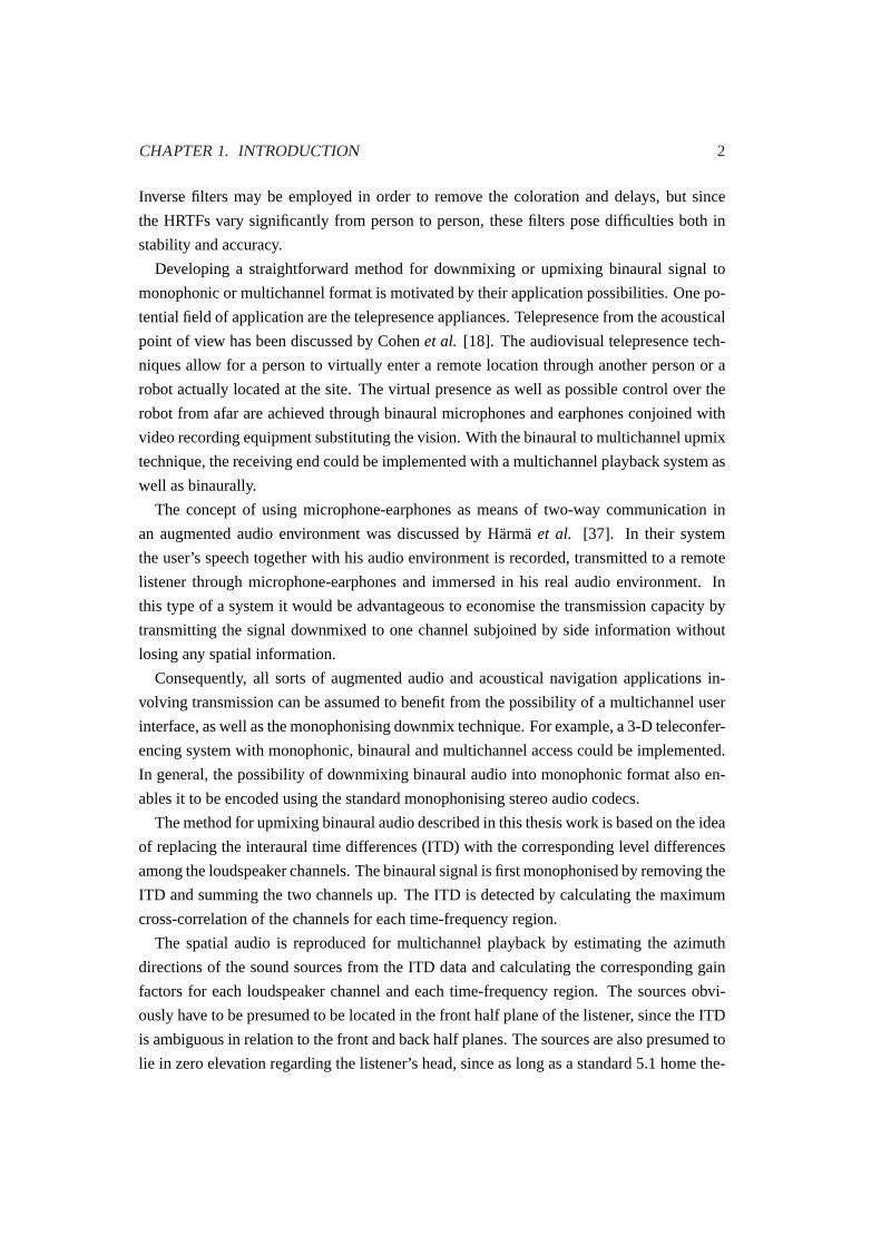
The method for upmixing binaural audio described in this thesis work is based on the idea
of replacing the interaural time differences (ITD) with the corresponding level differences
among the loudspeaker channels. The binaural signal is first monophonised by removing the
ITD and summing the two channels up. The ITD is detected by calculating the maximum
cross-correlation of the channels for each time-frequency region.
The spatial audio is reproduced for multichannel playback by estimating the azimuth
directions of the sound sources from the ITD data and calculating the corresponding gain
factors for each loudspeaker channel and each time-frequency region. The sources obvi-
ously have to be presumed to be located in the front half plane of the listener, since the ITD
is ambiguous in relation to the front and back half planes. The sources are also presumed to
lie in zero elevation regarding the listener’s head, since as long as a standard 5.1 home the-
CHAPTER 1. INTRODUCTION 3
ater type multichannel playback is considered, no elevations can be rendered anyway. The
monophonic signal is then panned by using the gain factors and fed to the loudspeakers.
The system is naturally not audibly transparent, since the original source signal quality
cannot be recovered. This is due to the individuality of the HRTFs in the binaural record-
ings. The avoiding of inverse filtering leaves the processed signal coloured, mainly low-pass
filtered, depending on the direction of the source. The coloration can, however, be reduced
to some point with equalising filters.
The quality problem of the processed audio, together with the cone of confusion restric-
tion, set constraints on the appliances of the upmix technique. They are thus set in the scope
of the future work.
This thesis is structured as follows: The two following chapters introduce the theory and
earlier work on which the method developed in this thesis bases upon. Chapter 2 presents
the basic theory of human spatial hearing as well as the existing methods for artificial az-
imuth estimation. In chapter 3 the theory and methods of upmixing and downmixing the
audio signal for different playback systems are discussed.
Chapter 4 introduces the new upmix method, and chapter 5 accounts for the testing
arrangements as well as the results of the testing. Chapter 6 presents the conclusions of
this thesis as well as point the direction for future work.
Chapter 2
Spatial hearing and azimuth
estimation
To begin the theoretical part of the thesis, the basics of binaural spatial hearing are discussed
briefly. Since the most common multichannel playback layout is the standard 5.1 system,
the relevant dimension of the source location estimation in the upmix can be assumed to
be the lateral one. Thus, the emphasis of the chapter is on azimuth estimation, i.e. the
localisation of sources in the horisontal plane. Section 2.1 covers the basics of binaural
localisation from the point of view of human hearing, whereas the methods for azimuth
estimation, that is the modelling point of view, are discussed in section 2.2.
2.1 Binaural localisation cues
Our ablility to localize sound sources is based on the physical distance of our two ears,
which causes the sound to arrive at them slightly differently. The filtering effect of the
head, torso and ears causing the differences is thoroughly described by the Head-Related
Transfer Functions (HRTFs). An HRTF is defined as the transfer function measured from a
sound source in free field to the ear of a human or an artificial head, divided by the transfer
function to a microphone replacing the head and placed in the middle of the head. The
HRTFs are individual, depending on the shape and size of the head and the torso of the
listener, as well as the shape and placement of the ears, and are thus impossible to model
accurately. An extensive textbook of spatial hearing is written by Blauert [10].
There are several types of localisation cues that can be specified. The cues that the
human hearing interprets from the sound at one ear are calledmonaural cues. These cues
contribute mainly to the definition of the median plane, elevation angle and distance of
the sound source. Theinteraural cues, referring to the differences between the two ear
4
CHAPTER 2. SPATIAL HEARING AND AZIMUTH ESTIMATION 5
signals, contribute mainly to the azimuthal localisation. The interaural cues are discussed
in section 2.1.1, whereas the other cues, including monaural cues, are briefly described in
section 2.1.2. Section 2.1.3 deals with the processes of human hearing of combining the
information of the different cues, and section 2.1.4 discusses the localisation capability in
the presence of multiple sources.
2.1.1 Interaural cues
According to Lord Rayleigh’s duplex theory [78], the two most important localisation cues
that can be segregated from the HRTFs are the Interaural Level Difference (ILD) and the
Interaural Time Difference (ITD). When a sound source is located to the side of the head,
there is a difference in the distance the sound has to travel in order to reach the two ears.
This will cause the sound to be both attenuated and delayed at the contra-lateral ear, i.e. at
the ear further away from the source, in relation to the sound at the ipsi-lateral ear, i.e. at
the ear closer to the source. Furthermore, reflections, diffraction and resonances caused by
the head, torso and the external ears of the listener affect the spectra of the signals arriving
to the two ears. The spectral differences, depending on both direction and frequency, are
referred to as ILD, or in some occasions Interaural Intensity Difference (IID) or Interaural
Amplitude Difference (IAD), and are measured to be up to approximately 6 dB. The ILD
is the main localisation cue at the frequencies above approximately 1.5 kHz, as the lower
frequency sound waves travel through the head and are thus not substantially attenuated
[10].
The ITD, which defines the difference in the arrival time of sound at the two ears, is the
main localisation cue at the frequencies below 1.5 kHz. At frequencies where the wave-
length of the signal is greater than the distance between the ears, the delay can be uniquely
determined from the phase difference between the ears. At higher frequencies, however, the
delay is ambiguous. The boundary frequency of 1.5 kHz describes rather a transition region
than a precise value, and it is in any case highly approximate since it is derived from the
distance between the two ears. The diameter of an average human adult head is generally
considered to be approximately 21 cm, which corresponds to a measured delay of 630µs at
90 degrees sound incidence, and thus to the frequency of approximately 1.5 kHz [10]. The
term Interaural Phase Difference (IPD) is sometimes used instead of ITD.
The resolution of the localisation is at its best in the front median plane near the median
axis, the absolute lower limit for the localisation blur being about 1 degree [10]. However,
most of the localisation problems occur also in the median plane, where both the ITD and
the ILD are close to zero. Furthermore, problems occur on thecone of confusionwhere
both the ITD and ILD cues are ambiguous. Figure2.1 shows the cone of confusion. Re-
search shows that in these situations, especially in the case of narrow-band signals, the
CHAPTER 2. SPATIAL HEARING AND AZIMUTH ESTIMATION 6
source tends to be located incorrectly, in the direction axially symmetric with respect to
the axis of the ears. The phenomenon, commonly called thefront-back confusion, disap-
pears when the bandwidth of the signal is increased, the spectra of the ear input signals
giving enough monaural localisation information. In addition to the increased bandwidth,
increased duration and familiarity of the signal aid in the localisation [10].
Figure 2.1:The cone of confusion denotes the circle from where the relative distance to the
two ears stays equal. Sources that lie on this circle give equal interaural localisation cues.
2.1.2 Other localisation cues
It has been shown that the two main interaural localisation cues contribute primarily to the
identification of lateral displacements, whereas monaural cues, such as level differences
within the spectrum caused mainly by the pinna, serve primarily in defining the median
plane, elevation angle, and distance of the sound source [6].
In addition to the aforementioned, a number of further localisation cues are available.
The room acoustic cues, especially the early reflections, have been found to enhance the
spatial orientation. It has been found that a more or less unconscious movement of the head
is characteristic when trying to localise a sound source [43, 10]. The relative changes in
the interaural cues, as well as bringing the source into the region of sharpest hearing, that is
to the front, decrease the localisation blur. The influence of cues, such as the sound source
being visible to the subject, or the vibration perceived by other parts of the body besides the
ears, are explained by thevisualandtactile theories, respectively (see, [10]).
2.1.3 Combining the information given by different cues
When the information from different cues conflicts, human hearing tends to choose and rely
on the cues that give more consistent and credible information and ignore the implausible
information [85]. For example, in the case of noisy or reverberant acoustic environment,
where the additional sounds or reflections of the source sound from the walls and floor alter
CHAPTER 2. SPATIAL HEARING AND AZIMUTH ESTIMATION 7
the signals at the ears, the low-frequency ITD cues have been found to dominate the source
localisation through theprecedence effect[84]. It has been shown that if the onset of the
sound is clear, the hearing tends to fix on the angle of incidence of the first sound arriving to
the ears. This is especially important in a room acoustical situation where the direct sound
from the source is followed by reflections from multiple directions. The phenomenon is
called theHaas effector the precedence effect [82, 88, 33]. On the other hand, if for
example binaural recordings are listened to through loudspeakers, the sources are usually
correctly localised on the basis of level differences, though the ITD causes spatial distortion
in the sensation.
2.1.4 Multiple sound sources
When there are multiple sound sources present, they may be perceived either as a single
auditory event whose location is determined through superposition principle, or as separate
events connected to the congruent sources [10]. The result depends on the degree of coher-
ence of the signals radiated from the sources. Two signals are defined coherent if they are
identical or if they differ in level or phase delay independently of frequency. The interaural
coherence measure is widely employed in modelling the human source localisation [25] as
well as in audio upmix techniques [3].
If the source signals, e.g. the signals of two loudspeakers, are at least nearly coherent,
then only a single source called aphantom sourceor avirtual sourceis perceived. The loca-
tion of the phantom source depends on the level and phase difference between the summed
signals at the two ears. Of these cues, the level difference is commonly used as the basis of
stereo sound production. The location of the phantom source is related to the signal gains
at the two loudspeakers through thestereophonic law of sinesintroduced by Blumlein [11],
and more closely discussed in chapter 3.
If the delay between the signals from the two sources exceeds about 1 ms, the location
of the source is in most cases determined only by the location of and the signal radiated
by the source from which the signal arrives at the ears first. The localisation information
in the signal arriving later is suppressed by the hearing in the interpretation process. This
phenomenon is calledthe law of the first wavefrontand it is closely related to the prece-
dence effect. If the delay is even considerably longer, the limit depending on the listening
conditions, two separate auditory events are perceived. The signal from the latter source is
then perceived as an echo of the former source. This relates to the image source theory (see
[2]), where calculation of sound fields is simplified by understanding echoes, or reflections
of the sound from boundaries, as signals from secondary sources located boundary-wise
symmetrically to the primary source.
Multiple sources are perceived as separate auditory events also when the waveforms of
CHAPTER 2. SPATIAL HEARING AND AZIMUTH ESTIMATION 8
the signals radiated from the sources are not equal, i.e. when the level and / or time dif-
ference between the signals is dependent of frequency. The human hearing is amazingly
skilled in distinguishing sources even with minor differences. An example is a symphony
orchestra concert where the listener is able to distinguish the sounds of different instruments
relatively easily. Another example is our ability to focus attention on one speaker amidst
a din of voices, even without turning towards the speaker. The phenomenon is commonly
known as thecocktail party effectand it was introduced by Cherry [16]. Simulating the
effect still remains a great challenge, but it has been proved that it is essentially dependent
of binaural hearing.
In addition to employing binaural cues, the hearing tends to distinguish multiple si-
multaneous sound sources by assosiating certain signal components as coming from the
same source according to their spectral characteristics. The process of identifying separate
sources from the complex acoustic environment is studied inauditory scene analysis, a
concept created by Bregman and extensively explained in [13]. In the source signal distin-
guishing process, learning as well as the visual perception play considerable roles.
Sources can be distinguished as long as none of them are masked by others. A signal
may be masked by another signal or noise when their level difference exceeds a certain
limit depending on their frequency composition. The masking effect is more extensively
explained in the next section.
2.2 Methods of azimuth estimation
In artificially estimating source azimuths from binaural signal, the ITD and ILD are the two
most important cues. The HRTFs as such do not work well in the estimation since they
are individual and thus impossible to interpret both accurately and generally at the same
time. According to the duplex theory described earlier, for narrow band signals, ITD is the
dominant cue at low frequencies, whereas ILD cues dominate at the high frequencies. To
pursue accurate analysis, the signal is decomposed into segments both frequency-wise and
time-wise. Furthermore, when environmental noise and spatial reverberation are present in
the binaural signal, precedence effect modelling can be used to enhance the estimation.
In estimation methods of moderate complexity, other localisation cues are in general not
used. The frequency and temporal analysis are discussed in section 2.2.1, and the derivation
of azimuth estimates from the ITD and the ILD is covered in section 2.2.2. Section 2.2.3
explains the precedence effect modelling and section 2.2.4 describes essential implementa-
tions of azimuth estimation.
CHAPTER 2. SPATIAL HEARING AND AZIMUTH ESTIMATION 9
2.2.1 Frequency and temporal analysis
In order to imitate the analysis methods of human hearing, a binaural wideband signal is
generally divided into frequency bands. Thecritical bandwidth theory(see, e.g. [89]) ex-
plains the resolution of hearing of wideband signals with an auditory filter of which the
width is dependent on the center frequency, i.e. the position at the cochlea. A critical band
defines the smallest band of frequencies which activate the same part of the basilar mem-
brane at each center frequency. The widths of the bands have been defined with different
scales, of which the Equivalent Rectangular Bandwidth (ERB) scale [59] is commonly be-
lieved to be the most accurate. The width of an ERB band (in Hz) is typically 11-17% of
the center frequency. One ERB band, as a function of center frequencyfc in Hz, can be
calculated with equation
∆fERB = 24.7 + 0.108fc (2.1)
A filter bank implementing the ERB scale, often called thecochlear filter bank, can be
realised with gammatone functions defined by the equation [76]
g(t) = atn−1e−2(fc)t cos(2ct + θ) (2.2)
whereatn−1 defines the start of the response,b(fc) is the bandwidth of the ERB band in
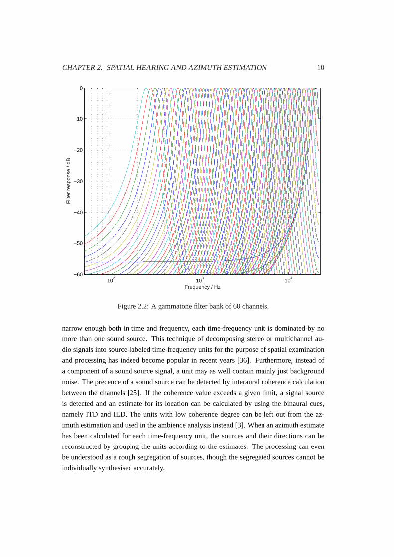
Hz, andθ is the phase. Figure2.2 shows the magnitude response of a gammatone filter
bank of 60 filters, which corresponds to ERB bands at the sampling frequency of 44.1 kHz.
The time resolution of human hearing is an even more complex phenomenon than the
frequency resolution. The monaural resolution has been measured to be approximately 1-
2 ms, depending on the type of the stimulus [10]. This means that if the time difference
between the two consequent sound events is less than 1-2 ms, they are perceived as one
sound. However, the temporal integration behaviour of the hearing, causing among others
the masking effect, tends to affect on the order of 100-200 ms. The size of the time frames
used in the azimuth analysis is chosen both on basis of the physiology of hearing, as well
as the requirements of efficient computation. If the frames are too short, the signal analysis
will suffer from inaccuracy due to too few samples per frame. Longer frames, both lower
the resolution of the analysis and cause the processing to lag, which may be unacceptable
regarding the implementation. It is common to use overlapping frames so as to achieve a
smooth transfer between the frames.
Interestingly enough, now that the signal is divided into frequency bands and time frames,
i.e. time-frequency regions, the aforementioned masking can be taken advantage of in the
analysis. According to Moore (see, [58]), a stronger signal masks the weaker ones within
the same critical band as well as within temporal vicinity. Thus, required that the units be
CHAPTER 2. SPATIAL HEARING AND AZIMUTH ESTIMATION 10
102
103
104
−60
−50
−40
−30
−20
−10
0
Frequency / Hz
Filt
er r
espo
nse
/ dB
Figure 2.2:A gammatone filter bank of 60 channels.
narrow enough both in time and frequency, each time-frequency unit is dominated by no
more than one sound source. This technique of decomposing stereo or multichannel au-
dio signals into source-labeled time-frequency units for the purpose of spatial examination
and processing has indeed become popular in recent years [36]. Furthermore, instead of
a component of a sound source signal, a unit may as well contain mainly just background
noise. The precence of a sound source can be detected by interaural coherence calculation
between the channels [25]. If the coherence value exceeds a given limit, a signal source
is detected and an estimate for its location can be calculated by using the binaural cues,
namely ITD and ILD. The units with low coherence degree can be left out from the az-
imuth estimation and used in the ambience analysis instead [3]. When an azimuth estimate
has been calculated for each time-frequency unit, the sources and their directions can be
reconstructed by grouping the units according to the estimates. The processing can even
be understood as a rough segregation of sources, though the segregated sources cannot be
individually synthesised accurately.
CHAPTER 2. SPATIAL HEARING AND AZIMUTH ESTIMATION 11
2.2.2 Estimating azimuth from ITD an ILD
The estimation methods usually employ either ITD alone, or a combination of ITD and
ILD cues. Azimuth estimates based on ITD are more accurate but unambiguous only at low
frequencies. They are calculated using the Cross-Correlation Function (CCF) based on the
theory by Jeffress [39]: The delay between the signal arriving at the two ears corresponds to
the index of the maximum of the CCF. The Jeffress model was probably the first localisation
model ever published. In fact, later, evidence of cross-correlation-like neural processing has
been found in physiological studies of the human hearing [87].
At higher frequencies, the wrapping of phase causes the CCF to give multiple maxima,
which causes the ITD to be ambiguous. However, the envelopes of the signals, derived by
using the Hilbert transform, can be employed at these frequencies, so as to avoid the ambi-
guity [53, 10, 72]. In good listening conditions highly accurate estimates can be achieved
by using the ITD only [49, 15].
There is a variety of ways for deriving azimuth estimates from the ILD and combining
them with the ones from the ITD. One method is to calculate the logarithm of the zero-lag
autocorrelation of each frequency channel to approximate the amplitude spectrum by using
channel-by-channel differences to obtain a measure of the ILD spectrum in decibels [49].
The problem in this approach is that in addition to the azimuth, frequency and elevation
affect the results. A better method is to calculate the signal energies in segments of the filter
band outputs for each ear [51]. The ILD is then calculated as the ratio of the energies of the
two channels in decibels. When the filters are sharp enough and given that the measurement
is of energy ratio, the result can be presumed independent of the spectrum of the source.
Furthermore, the estimate from the ILD can be employed only in solving the phase ambi-
guity of the ITD at high frequencies, as in [81]. An efficient way for the source location
analysis often used is to apply look-up tables for the ITD and ILD values. The tables can
be implemented as self-learning or prelearned maps, as in [51].
As long as only ITD and ILD are used in the estimation, the source has to be assumed in
the front (or back) half plane and at the azimuth level, i.e. at the level of the listener’s ears.
This is due to the cone of confusion where both cues give ambiguous information. Con-
sequently, most azimuth estimation implementations are restricted to the frontal azimuth
angles. The area of operation can be extended by using additional cues such as detecting
head movements with a head-tracker [37], but this significantly adds to the complexity of
the system. In most cases, it is reasonable to presume the sound source to be in the frontal
horizon, since the listener can be assumed to turn his head towards the sound.
CHAPTER 2. SPATIAL HEARING AND AZIMUTH ESTIMATION 12
2.2.3 Appliance of azimuth estimation
Azimuth estimation methods have been developed for a variety of purposes. In general,
the front-back confusion cannot be solved when only ITD- and ILD-based estimates for
azimuth are used, and thus it is in most cases presumed that the sound source lies in the
front half plane.
A computer model for frontal plane azimuth estimation was developed by Pocock [65].
The model is strongly founded on imitating the physiology of human hearing, and it is
the basis of several implementations, such as the stereo imaging measurement model by
Macpherson [51]. Azimuth estimation is used in binaural source separation by Viste and
Evangelista [81], and in missing data speech recognition by Palomäkiet al. [62]. It is also
used in simulating the cocktail party effect with a speech segregation method by Romanet
al. [72].
Chapter 3
Upmix and downmix
Audio upmix and downmix techniques are being developed since the traditional home
stereo system is no longer the dominant medium for audio playback. The direction of
progress is illustratively reflected in the objectives of audio codec development, which is
striving for transparent codecs capable of serving anything from a variety of multichannel
loudspeaker layouts to mobile playback devices employing headphones or earphones. At
the same time, the key to efficient transmission of audio through any medium is to downmix
it (with minimum loss of information) into as few channels as possible.
Another motivation for the development of upmix and downmix techniques is that the
equipment and setups needed for recording directly into binaural or different multichannel
formats are not at all straightforward. The traditional stereo recording methods, however,
are widely used and generally well mastered. Diverse mixing techniques allow for a single
recording to be played back with any type of equipment, fully utilising the characteristic
capacity of the playback equipment.
This chapter overviews the existing upmix and downmix techniques and motivates the
development of a technique for upmixing binaural audio into the multichannel format. The
variety of audio content types, as well as panning techniques supporting them, are discussed
in section 3.1. Upmix and downmix techniques between different loudspeaker composi-
tions are reviewed in section 3.2, and section 3.3 performs the congruent review for mixing
between loudspeaker and binaural or headphone formats.
3.1 Binaural and multichannel audio contents and panning tech-
niques
The multichannel reproduction of audio has gained extensive popularity in the form of home
theater systems recently and the techniques and devices have been developed rapidly. Since
13
CHAPTER 3. UPMIX AND DOWNMIX 14
the content of multichannel audio varies greatly from the diversity of music categories all
the way to movie soundtracks and virtual environments, there is no unique way of mixing it
between the loudspeaker channels. A variety of microphones and recording techniques have
been developed for multichannel recording, some of them introduced in the next paragraphs.
Nonetheless, storing up to six, or even more, audio channels instead of two, is expensive
and inefficient. Added that practically all of the excisting recordings are in stereo format
anyway, a demand for efficient and high-quality upmix/downmix and coding techniques
exists.
The different types of audio content are overviewed in section 3.1.1. In the following sec-
tions, the spatial audio recording and reproduction methods are divided in three categories:
Discrete panning techniques are covered in section 3.1.2, sound field reconstruction tech-
niques are covered by section 3.1.3, and head-related stereophony is discussed in section
3.1.4.
3.1.1 Audio contents
The creation of audio content begins by recording or synthesising the sound material. A
traditional recording method has been a stereophonic microphone pair, directly compatible
with stereophonic loudspeaker reproduction. When recording for example music in studio
conditions, the sound sources are generally recorded one by one on separate tracks. This
enablesdiscrete panningof the signals, i.e. the processing of each track individually, and
then conjoining them in desired proportions into a stereo or multichannel signal. Another
approach to recording is to use an omnidirectional Soundfield microphone [26], or a set of
directional microphones, and measure the sound pressure field in a reference point. The
aim is thesound field reconstructionat the reference point by feeding a set of loudspeakers
with loudspeaker signals calculated from the measured signals through matrixing. A third
approach is binaural recording, orhead-related stereophony, where the acoustic pressure is
measured in the ears of a listener or a dummy head with small-sized probe microphones.
The equal acoustic pressure is then reproduced in the ears through headphone or loud-
speaker playback.
Besides recording, the audio material can naturally be created through synthesis, em-
ploying the aforementioned approaches. This classification of spatial audio encoding and
reproduction techniques into the three aforementioned categories was introduced by Jotet
al. [42]. According to them, the approaches yield different tradeoffs between several design
criteria, including fidelity of the directional and timbral reproduction, complexity in terms
of number of channels or signal processing, as well as freedom of movement of the listener
and size of the listening area. The type of application thus determines the selection of one
technique over another.
CHAPTER 3. UPMIX AND DOWNMIX 15
Considering music reproduction, Avendano and Jot have identified two different ap-
proaches to mixing music [4]. In the so calleddirect/ambientor in the audienceapproach,
the different sources, e.g. instruments, are panned among the front channels in a frontally
oriented fashion, and the ambience components of the signal are distributed among all chan-
nels enriching the essentially stereophonic mix. In thein the bandapproach, the sources as
well as the ambience signals are panned among all the loudspeakers, creating the impression
that the listener is surrounded by the musicians.
For movie soundtracks, the de facto standard is to mix the dialogue in the center chan-
nel, music and other audio environment in the left and right front channels, and ambience
noise type sound in the surround channels. All the available channels are naturally used
when for example a moving sound source goes around the scene. In some systems, the
omnidirectional low-frequency effects are mixed in the LFE channel, intended to be played
back through a subwoofer. The advance of using the center channel instead of the left and
right front channels for dialogue is that the area of listening where it will appear to be com-
ing from the center, that is where the movie picture is located, is considerably larger. The
weakness of the phantom sources, created pairwise between adjacent loudspeakers, is that
if the listener moves out from the so called sweet spot, towards one of the loudspeakers,
the stereo image will collapse into the loudpeaker closest to the listener. By using a third
loudspeaker in the center, a larger and more robust sweet spot can be achieved, fitting more
people in the audience [79].
3.1.2 Discrete panning techniques
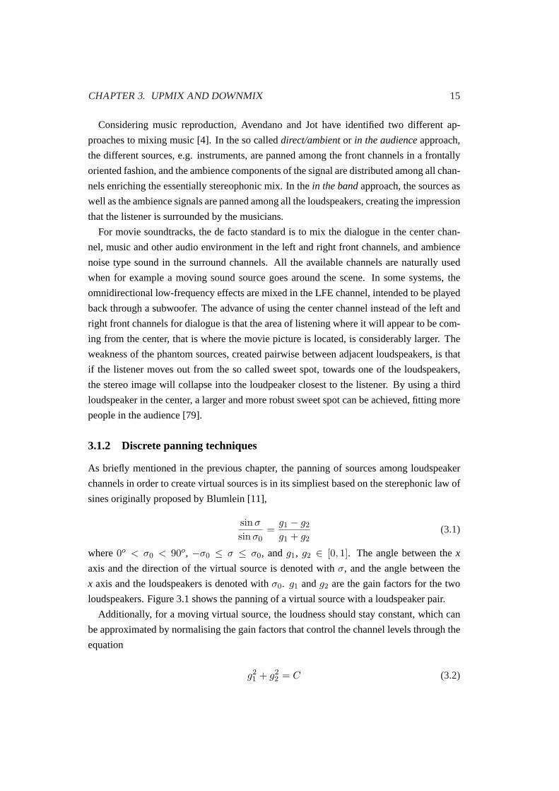
As briefly mentioned in the previous chapter, the panning of sources among loudspeaker
channels in order to create virtual sources is in its simpliest based on the sterephonic law of
sines originally proposed by Blumlein [11],
sinσ
sinσ0=
g1 − g2
g1 + g2(3.1)
where0o < σ0 < 90o, −σ0 ≤ σ ≤ σ0, andg1, g2 ∈ [0, 1]. The angle between thex
axis and the direction of the virtual source is denoted withσ, and the angle between the
x axis and the loudspeakers is denoted withσ0. g1 andg2 are the gain factors for the two
loudspeakers. Figure3.1shows the panning of a virtual source with a loudspeaker pair.
Additionally, for a moving virtual source, the loudness should stay constant, which can
be approximated by normalising the gain factors that control the channel levels through the
equation
g21 + g2
2 = C (3.2)
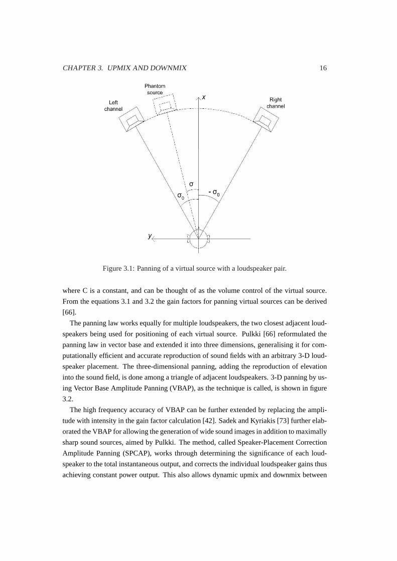
CHAPTER 3. UPMIX AND DOWNMIX 16
Figure 3.1:Panning of a virtual source with a loudspeaker pair.
where C is a constant, and can be thought of as the volume control of the virtual source.
From the equations3.1and3.2 the gain factors for panning virtual sources can be derived
[66].
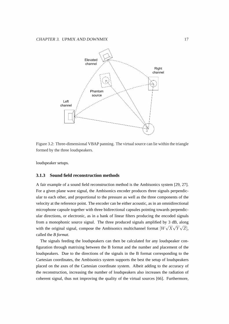
The panning law works equally for multiple loudspeakers, the two closest adjacent loud-
speakers being used for positioning of each virtual source. Pulkki [66] reformulated the
panning law in vector base and extended it into three dimensions, generalising it for com-
putationally efficient and accurate reproduction of sound fields with an arbitrary 3-D loud-
speaker placement. The three-dimensional panning, adding the reproduction of elevation
into the sound field, is done among a triangle of adjacent loudspeakers. 3-D panning by us-
ing Vector Base Amplitude Panning (VBAP), as the technique is called, is shown in figure
3.2.
The high frequency accuracy of VBAP can be further extended by replacing the ampli-
tude with intensity in the gain factor calculation [42]. Sadek and Kyriakis [73] further elab-
orated the VBAP for allowing the generation of wide sound images in addition to maximally
sharp sound sources, aimed by Pulkki. The method, called Speaker-Placement Correction
Amplitude Panning (SPCAP), works through determining the significance of each loud-
speaker to the total instantaneous output, and corrects the individual loudspeaker gains thus
achieving constant power output. This also allows dynamic upmix and downmix between
CHAPTER 3. UPMIX AND DOWNMIX 17
Figure 3.2:Three-dimensional VBAP panning. The virtual source can lie within the triangle
formed by the three loudspeakers.
loudspeaker setups.
3.1.3 Sound field reconstruction methods
A fair example of a sound field reconstruction method is the Ambisonics system [29, 27].
For a given plane wave signal, the Ambisonics encoder produces three signals perpendic-
ular to each other, and proportional to the pressure as well as the three components of the
velocity at the reference point. The encoder can be either acoustic, as in an omnidirectional
microphone capsule together with three bidirectional capsules pointing towards perpendic-
ular directions, or electronic, as in a bank of linear filters producing the encoded signals
from a monophonic source signal. The three produced signals amplified by 3 dB, along
with the original signal, compose the Ambisonics multichannel format[W√
X√
Y√
Z],called theB format.
The signals feeding the loudspeakers can then be calculated for any loudspeaker con-
figuration through matrixing between the B format and the number and placement of the
loudspeakers. Due to the directions of the signals in the B format corresponding to the
Cartesian coordinates, the Ambisonics system supports the best the setup of loudspeakers
placed on the axes of the Cartesian coordinate system. Albeit adding to the accuracy of
the reconstruction, increasing the number of loudspeakers also increases the radiation of
coherent signal, thus not improving the quality of the virtual sources [66]. Furthermore,
CHAPTER 3. UPMIX AND DOWNMIX 18
at the high frequencies optimal localisation criteria leads to non-linear equations, impossi-
ble to solve through matrixing for other than regular loudspeaker layouts. In such cases,
numerical optimisation is required [42].
The microphone technique, employed among other sound field reconstruction methods
in the Ambisonics recording, is coincident microphone technique, where directive micro-
phones are positioned as close to each other as possible [29, 50]. The sound signal is thus
captured in the same phase by all the microphones. If the number and directions of the mi-
crophones correspond to the loudspeaker layout, in the best occation the loudspeakers can
be fed directly by the recorded signals without any processing. The number of microphones
is however limited by their physical size and directivity. The coincident microphone tech-
niques are able to produce the sharpest virtual sources. In the non-coincident microphone
techniques, omnidirectional or directional microphones are placed at a distance of each
other, capturing the sound signal in different phases. This type of techniques are found to
create a better feeling of ambience, and the reproduction is also less sensitive to the location
of the listener, at the cost of lower directional accuracy [67].
Another example of sound field reconstruction methods is thewave field synthesispro-
posed by Berkhout al. [7, 8], where individual loudspeakers are replaced by loudspeaker
arrays in order to generate wave fronts from the intended sources. This method allows the
rendering of the original wave field in the entire listening space instead of a limited sweet
spot. To produce the wave field, the listening area is surrounded with linear loudspeaker ar-
rays, in the ideal case loudspeaker planes. The loudspeakers are fed with signals producing
a volume flux proportional to the normal component of the particle velocity of the origi-
nal sound field at the corresponding position. The wave field synthesis method has been
reported to perform well for reconstructing both discrete sources and diffuse sound fields
[35]. However, the practicality of the method, especially for home use, can be impugned
due to the requirements for the amount and placing of the equipment.
3.1.4 Head-related stereophony
In the binaural synthesis methods, the intention is to reconstruct the pressure field created
by the original source signal at the ear drums of the listener. The methods base on the
utilisation of the Head-Related Transfer Functions, introduced in the previous chapter. A
set of Head-Related Impulse Responses is created by measuring the impulse responses for
a wideband sound from a discrete series of directions at the left and right ear of a test
subject or an artificial head. An artificial, or dummy head, is a measurement microphone
specifically constructed to simulate an average human head and torso. Sound material can
then be spatially synthesised by convolving it with the HRIRs. In order to keep the virtual
environment static while the listener moving his head, real-time head tracking is required. If
CHAPTER 3. UPMIX AND DOWNMIX 19
the intention is to synthesise virtual sources in the current listening space, the source signal
recordings need to be done in an anechoic chamber and the room response has to be added
by measuring or modelling the Binaural Room Impulse Response (BRIR) of the space and
updating it in relation to the movements of the listener and the source [10].
Since all the convolutions and interpolations of the long impulse responses typically lead
to unacceptably heavy processing, much work has been done on eliminating everything
perceptually less relevant from the calculation. To begin with, the HRTF database can be
reduced considerably by dividing the impulse responses into a minimum-phase and all-pass
components, that is separating the ITD to be stored as a pure delay. Depending on other
rationalisation procedures and the angles of incidence, the lengths of the impulse responses
can be substantially reduced [38]. Storage capacity can be further saved by assuming that
the impulse responses for left and right ear are symmetrical. Thus, whenever the impulse re-
sponse for angleσ is used in convolution of the left ear signal, the left ear impulse response
for angle360o − σ can be used in convolution of the right ear signal, and thus there is no
need for storing the right ear impulse responses. Furthermore, the requirement for process-
ing capacity can be brought down by replacing the calculation of accurate room response
with moderate reverberation simulation. It has been found that adding a generic reverbera-
tion to binaurally synthesised sound substantially improves the spatialisation of the sound
image [10, 45]. Aspects of binaural synthesis are extensively discussed for example in
[32, 41, 42].
The advantages of binaural synthesis include the prospect of competent spatialisation
generated with reasonably light, even portable equipment, and listening environment not
affecting the quality of the reproduction. Yet, common problems in binaural synthesis are
the front-back confusion, insufficient in-front localisation, coloration and poor externali-
sation of the sound [35]. Furthermore, the playback is restricted to a single listener. The
overly massive requirements for processing capacity practically prohibit any real-time ap-
plications of binaural synthesis.
3.2 Upmix and downmix techniques for different formats of loud-
speaker audio
There is currently a lot of effort put in multichannel audio coding and compression with
a special interest on compatibility among any kind of loudspeaker setups. Allowing high-
quality real-time upmix and downmix, the required storing and transmission capacity for
audio content can be substantially reduced. Sections 3.2.1 and 3.2.2 discuss the existing
upmix and downmix techniques between monophonic and stereophonic audio, respectively.
Section 3.2.3 covers techniques that allow upmix and downmix of audio signal between
CHAPTER 3. UPMIX AND DOWNMIX 20
monophonic and stereophonic reproduction as well as any layout of loudspeakers.
3.2.1 Monophony to stereophony upmix
Stereo sound reproduction was first experimented with already in the early 1900’s, and
gained widespread popularity in the 1950’s when the Stereo LP phonograph record was
introduced. Schroeder [74] employed different constructions of delay lines, bandpass filters
and allpass filters, and introduced the basic theory of upmixing monophonic sound into
stereophony. According to Schroeder, apseudo-stereophonic effectcan be obtained by
complementarily comb-filtering the mono signal for the two stereo channels.
Later, a model of astereo synthesiserbased on Schroeder’s theory was formulated by
Orban [61]. Two constraints were proposed for the synthesis: Firstly, the sum of the power
spectra of the left and right channels should be proportional to the power spectrum of the
mono input. Secondly, the magnitude of the sum of the left and right output channels should
be proportional to the magnitude of the mono input. These two constraints guarantee a
correspondence of perceived loudness between the synthesised stereo and the mono input,
as well as mono/stereo compatibility through lateral modulation. This way, Orban was able
to adjust the frequency spectra of the two channels, thus adding directionality instead of
mere diffusion. The frequency spectrum of one sound source could be placed towards the
left, while the others are placed towards the right, thus avoiding the "wandering" of sound
sources.
Since then, a variety of methods have been proposed in order to improve and fine-tune
the pseudo-stereo effect. Important aspects, such as simulating the distance as well as the
size of the sound sources, are discussed by Gerzon in [30]. Recently, the interest has turned
towards surround sound reproduction.
3.2.2 Stereophony to monophony downmix
The downmix of stereophonic sound into a single channel becomes interesting when the
economising of transmission capacity by encoding the signal to be transmitted is intended.
The simplest way of monophonising stereo sound is to take the average of the two channels,
i.e. dividing their sum by two. Here of course, it has to be taken into account that if a part
of the signal in the two channels is equal in magnitude but in opposite phase, it will be
cancelled out in the resulting signal. This method irriversibly loses all stereo information,
and the restoring the stereo signal will thus require pseudo-stereo synthesis described in the
previous section.
To date, there are more sophisticated techniques for coding stereophonic audio, aiming at
transparency, i.e. minimising the error between the restored and the original signals beyond
CHAPTER 3. UPMIX AND DOWNMIX 21
the sensitivity of human hearing. Simple and efficient methods widely used in perceptual
audio codecs are theSum/Difference (S/D) coding[40] and theIntensity stereo coding[34].
In the S/D coding the sum and difference of the left and right channel signals are encoded
instead of the two original signals. The adaptive codecs decide in time and for each fre-
quency band whether it is bitwise efficient to use S/D coding or to code the original two
signals as such. Intensity coding transmits for each coding band of the high frequencies
only the sum signal along with a scalar representing the energy distribution among chan-
nels. A popular approach are also the parametric coding methods, in which the idea is to
add, to the side of the monophonised audio channel, a bitstream of low bitrate delivering
the parameters describing the stereo image. The most recent advance in parametric stereo
coding can be viewed e.g. in [75] and [12].
3.2.3 Upmixing monophonic and stereophonic audio into multichannel for-mat
The development of surround sound technology began as early as before the World War II,
and from the very beginning, it has been driven by the movie industry [54]. Along with the
introduction of the Digital Versatile Disc (DVD), the3/2 format, consisting of left, center,
right, left surround and right surround channels, became supported by the film makers. In
the beginning of the 1990’s, the 5.1 configuration, introduced in their systems by bothDolby
Laboratories (Dolby Digitalfor home systems andDolby Digital Surroundfor cinemas)
and theDigital Theater Systems (DTS), became the de facto standard of loudspeaker layouts
for especially home multichannel stystems. The 5.1 configuration adds to the 3/2 format a
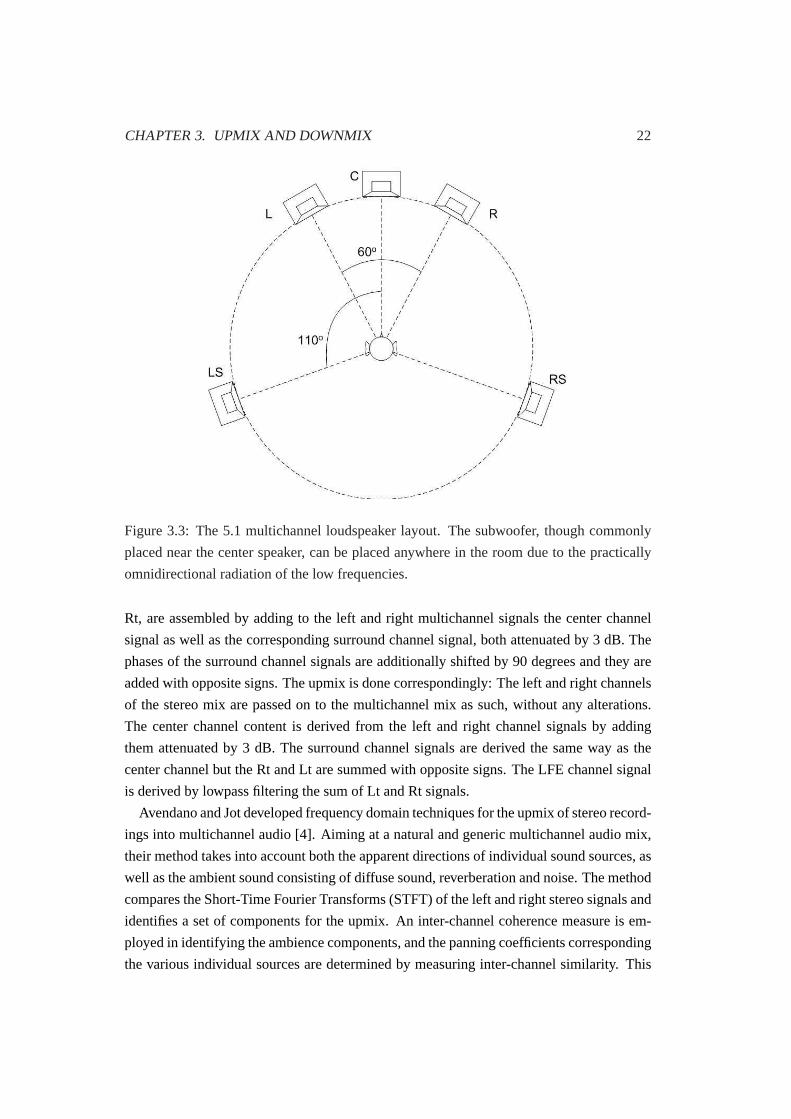
separate Low-Frequency Effects (LFE) channel for deep bass. Figure3.3 presents the 5.1
loudspeaker layout. Other layouts, such as the 7.1Sony Dynamic Digital Soundand the
6.1 Dolby Digital Surround EXare popular alternatives in cinema usage as well as in the
products of gaming technology.
One of the first surround sound recording and reproduction systems capable of handling
variable number of transmission channels as well as multiple loudspeaker layouts is the
Ambisonics system developed in the 1970’s, introduced earlier in this chapter. It was de-
veloped as a complete system taking care of everything from recording the sound material
all the way to reproducing it with any equipment at hand. Along with later systems, it is
still supported by many commercial products.
Dolby began introducing of the multichannel to stereo downmix feature in its codecs in
order to respond to the requirements of backwards compatibility. Additionally, Dolby Pro
Logic II includes the upmix from stereo back to 5.1 multichannel format. In the downmix,
the original source audio signals are encoded into two program channels, that can be played
back as stereo. The left and right stereo signals, called left-total and right-total, or Lt and
CHAPTER 3. UPMIX AND DOWNMIX 22
Figure 3.3:The 5.1 multichannel loudspeaker layout. The subwoofer, though commonly
placed near the center speaker, can be placed anywhere in the room due to the practically
omnidirectional radiation of the low frequencies.
Rt, are assembled by adding to the left and right multichannel signals the center channel
signal as well as the corresponding surround channel signal, both attenuated by 3 dB. The
phases of the surround channel signals are additionally shifted by 90 degrees and they are
added with opposite signs. The upmix is done correspondingly: The left and right channels
of the stereo mix are passed on to the multichannel mix as such, without any alterations.
The center channel content is derived from the left and right channel signals by adding
them attenuated by 3 dB. The surround channel signals are derived the same way as the
center channel but the Rt and Lt are summed with opposite signs. The LFE channel signal
is derived by lowpass filtering the sum of Lt and Rt signals.
Avendano and Jot developed frequency domain techniques for the upmix of stereo record-
ings into multichannel audio [4]. Aiming at a natural and generic multichannel audio mix,
their method takes into account both the apparent directions of individual sound sources, as
well as the ambient sound consisting of diffuse sound, reverberation and noise. The method
compares the Short-Time Fourier Transforms (STFT) of the left and right stereo signals and
identifies a set of components for the upmix. An inter-channel coherence measure is em-
ployed in identifying the ambience components, and the panning coefficients corresponding
the various individual sources are determined by measuring inter-channel similarity. This
CHAPTER 3. UPMIX AND DOWNMIX 23
technique is commercialised as the Creative MultiSpeaker System supported by a multitude
of multichannel computer sound cards.
The demand for ever greater compression efficiency, while preference shifting from
stereo to multichannel audio playback systems, inspired Faller and Baumgarte to develop
the Binaural Cue Coding (BCC) technique [24]. BCC is a parametric coding technique
capable of encoding any amount of source audio signals into a single audio signal accom-
panied by a low bitrate stream of metadata. At the receiving end, the corresponding decoder
generates from the mono signal and BCC bitstream multichannel audio signal for a play-
back system of similar or any other loudspeaker layout. The aim is that in the limits of
the playback system, the synthesised multichannel audio is perceptually similar to the orig-
inal multichannel audio. The parametrisation, describing the spatialisation of the audio,
is based on binaural localisation theory: The Inter-Channel Time Difference (ICTD) and
Inter-Channel Level Difference (ICLD) are calculated for each ERB frequency band and
each time frame of the signal.
The Spatial Impulse Response Rendering (SIRR) technique by Pulkkiet al. [68, 67] in
a way conjoins and extends the Ambisonics and BCC techniques in spatial reproduction of
measured room responses for arbitrary loudspeaker setups. The measuring of the room re-
sponse is done with a Soundfield microphone or a comparable system, and the reproduction
is based on analysing the direction of arrival as well as diffuseness of the measured sound at
frequency bands. In their listening test, the method performed remarkably well compared
to Ambisonics or reproduction of room response through diffusion.
3.3 Mixing between loudspeaker and headphone audio
While in loudspeaker reproduction of spatial audio, the panning of sources is usually done
by using level differences between the channels, in binaural reproduction the time differ-
ence between the channels is even more important than the level difference [10]. However,
using time differences in loudspeaker reproduction typically leads to extremely small sweet
spot, outside of which the spatial image distorts. The basics of upmix and downmix tech-
niques between monophonic and binaural audio are covered in section 3.3.1, and between
stereophonic and binaural audio in section 3.3.2. Downmix from multichannel to binaural
audio is discussed in section 3.3.3.
3.3.1 Mixing between monophonic and binaural audio
Binaural audio can be produced from monophonic signal by convolving the signal for each
ear with the HRTFs. The set of HRTFs consists of distinct transfer function for each possible
direction of sound. The data can be measured by using a set of test subjects and averiging
CHAPTER 3. UPMIX AND DOWNMIX 24
from their HRTFs a generic set of HRTFs, which is usually very time-consuming, expensive
and inaccurate since averiging highly individual data is not straightforward [57, 70]. Since
the dimensions of the ears vary among people, the peaks and notches they cause in the fre-
quecy response appear at different frequencies, and thus simple averiging would result in
rather flat transfer functions far from the truth. An easier, quicker and almost as accurate
way is to use a dummy head, such as the KEMAR [28] or the VALDEMAR [17], specif-
ically manufactured for acoustical measurements. Other artificial heads are discussed and
compared in [56]. There is a variety of measured databases available, of which probably
the most employed include the CIPIC database [1] and the KEMAR measurements [28].
To upmix monophonic audio into binaural format, information about the angle of inci-
dence of the sound source is needed. In case of multiple sound sources in various directions
within the recording, the sources need to be segregated in order to convolve each source
with the HRTF corresponding to its angle of incidence. The procedure is employed e.g. in
fully computed auralisation, where the sound field of a source in space is rendered audible
in order to simulate the binaural listening experience at a given point in a modeled space
[46].
The downmix from binaural to monophonic signal could be thought to be made by sim-
ply inverse filtering the binaural signals with the HRTFs. However, since the HRTFs are
individual, unless the HRTFs used in the upmix and downmix are the same, and possibly
even then, the filtering hardly leads to the original spectrum of the signal. A better way is
to simply sum the two ear signals. This method does not recover the original signal either,
but it is simpler and certainly stable.
3.3.2 Mixing between stereophonic and binaural audio
Since the two traditionally most popular ways of listening to commercial music recordings
are the stereo loudspeaker pair and the headphones, there has been effort in optimising the
spatial reproduction of stereo recordings for both. Although much improvement is achieved
through headphone design, also signal processing is employed in the process. The general
aim of the modification of audio for headphone listening is that of increasing the room
acoustical effect, which it is lacking compared to loudspeaker playback. In headphone and
earphone reproduction, compared to loudspeakers, the signal from each audio channel is
fed into one ear only, causing the components of the signal equal in both channels to be
localised in the middle of the head. Besides increasing the naturalness of the sensation, the
room acoustics also improve the out-of-head localisation or externalisation [10].
In earphone reproduction, the audio can be spatialised by employing the HRTFs. How-
ever, the headphones differ from the earphones in that the sound source is brought outside of
the outer ear instead of the ear canal. Using the HRTFs as such in headphone listening, the
CHAPTER 3. UPMIX AND DOWNMIX 25
signal arriving at the eardrum would be filtered by the outer ear twice. Hence, equalisation
is needed for listening binaural audio through headphones.
The use of HRTFs in headphone reproduction is generally restricted to modelling and
other research purposes due to the extensive generality and complexity challenges. More
common ways of improving the spatial sound image produced through headphones are the
use of crossfeed simulation and delay effects [80], as well as adding reverberation corre-
sponding to the listening space, such as a general-sized living room [45]. Examples of
commercial signal processing systems for binaural headphone enhancement are the BAP
Binaural Audio Processor by AKG Acoustics [69] and the Dolby Headphone [21].
Considering subsequently the opposite situation, namely the reproduction of binaural
audio through stereo loudspeakers, modification of the audio signal is even more needed.
The aim of binaural reproduction is to recreate exactly the same sound pressure at each
ear drum of the listener, that would be created by the original source in a real listening
situation. When binaural audio is reproduced through loudspeakers, the signal from the left
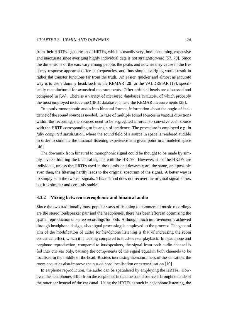
channel will leak into the right ear and vice versa, a phenomenon calledacoustic crosstalk.
Several acoustic crosstalk cancellation principles have been discussed in [55] and [47], the
simplified method being the addition of artificial crosstalk to the signal, which cancels out
the natural crosstalk.
3.3.3 Downmixing multichannel to binaural audio
The general approach to downmixing of multichannel audio into binaural format bases on
the virtual loudspeaker paradigm [42]. The two ear signals are constructed by superim-
posing the contributions of the individual loudspeakers weighted by their respective gain
factors. Kendallet al. used pairwise amplitude panning over 12 virtual loudspeakers sur-
rounding the listener in the horizontal plane [44]. More recently, the Ambisonic panning
technique has been proposed for the same purpose, since it allows both ambience recorded
with a Soundfield microphone to be used in the mixing, as well as compensating for the
rotations of the listener’s head after mixing by applying a rotation matrix [42]. When a dis-
crete set of HRTF filters is used, moving sources of continuously varying directions can be
reconstructed through interpolating between the filters. This approach is commonly called
local interpolation, whereas the Ambisonics techniques realise aglobal interpolationbased
on spherical harmonic decomposition and involving weighted contributions from all loud-
speakers in the system.
Chapter 4
Binaural to multichannel upmix
In this chapter a method for spatially reproducing binaural audio signal over a multichannel
loudspeaker system is described. The idea of the method is to convert the ITDs in the binau-
ral signal into corresponding amplitude differences among the loudspeaker channels. The
ILDs between the left and right ear signals are removed through monophonisation, while
the spectral coloration caused by them in the monophonised signal cannot be completely
removed.
The method is implemented with The MathWorks Matlab software, allowing easy imple-
mentation of mathematical functions, as well as versatile testing and plotting possibilities
during the development work. In the method, first, the binaural signal is monophonised and
the extracted spatial information is stored in a time-frequency matrix. Next, a gain factor for
each time-frequency unit of the monophonic signal for each playback channel is calculated
on the basis of the spatial information. The amplified signal is then fed to the loudspeak-
ers corresponding the playback channels. The first stage of the upmix method, that is the
estimation of the azimuth of the sound sources and the removal of the time delay between
the two channels, is explained in sections 4.1 and 4.2, respectively. Section 4.3 explains
the conversion of ITDs into azimuth angles, and section 4.4 accounts for the multichannel
upmix using the monophonic signal and the side-information matrix.
4.1 Azimuth estimation
The azimuth estimation in the method at issue, is based on the azimuth estimation method
employed in a missing data speech recognition technique reported by Palomäkiet al. [62].
In their technique, azimuth estimation, improved with precedence effect modelling, is em-
ployed in localising speech sources in a noisy environment, and it is based on theory and
methods developed by, among others, Darwin and Carlyon [20], Pattersonet al. [63] and
26
CHAPTER 4. BINAURAL TO MULTICHANNEL UPMIX 27
Martin [52]. The precedence effect modelling is also in the future plans of the upmix
method development. Opposed to the speech recognition method, in the upmix method
ILD information is not used in azimuth estimation, and the sampling frequency is set at
44.1 kHz instead of 20 kHz, in order to avoid artefacts caused by low sampling rate affect-
ing the listening test results.
To begin the upmix process, the binaural signal is filtered with a gammatone filter bank
of 59 channels. Simulating cochlear frequency analysis with a gammatone filter bank, to
date widely acknowledged, was proposed by Pattersonet al. [63] and it is implemented
here by employing the Auditory Tool Box for Matlab by Slaney [77]. The filter bank covers
the frequencies from 200 Hz to half the sampling rate. At frequencies below 200 Hz, both
the estimates given by the azimuth calculation, as well as the directional hearing ability
of humans decline. Consequently, it was decided to replace the gammatone filters with a
single low-pass filter at the lowest frequencies. A 500-tap FIR filter was used in this study
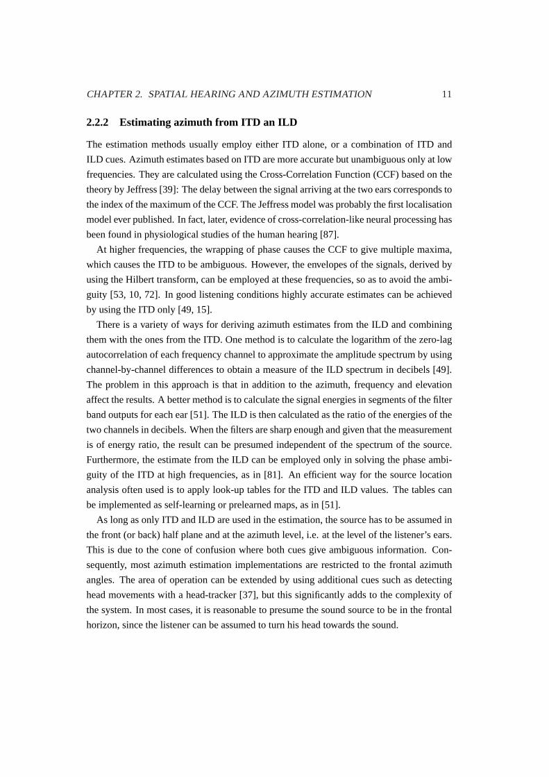
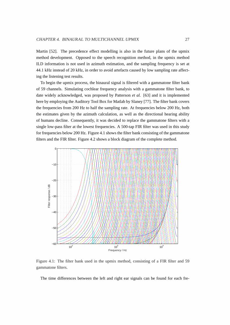
for frequencies below 200 Hz. Figure4.1shows the filter bank consisting of the gammatone
filters and the FIR filter. Figure4.2shows a block diagram of the complete method.
102
103
104
−60
−50
−40
−30
−20
−10
0
Frequency / Hz
Filt
er r
espo
nse
/ dB
Figure 4.1: The filter bank used in the upmix method, consisting of a FIR filter and 59
gammatone filters.
The time differences between the left and right ear signals can be found for each fre-
CHAPTER 4. BINAURAL TO MULTICHANNEL UPMIX 28
FILTER
BANK
60 CH
FILTER
BANK
60 CH
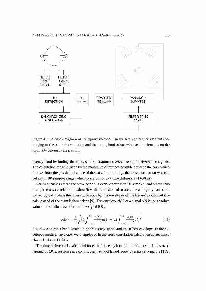
ITD
DETECTION
SYNCHRONIZING
& SUMMING
ITD
MATRIX
SPARSED
ITD -MATRIX
FILTER BANK
30 CH
PANNING &
SUMMING
Figure 4.2:A block diagram of the upmix method. On the left side are the elements be-
longing to the azimuth estimation and the monophonisation, whereas the elements on the
right side belong to the panning.
quency band by finding the index of the maximum cross-correlation between the signals.
The calculation range is given by the maximum difference possible between the ears, which
follows from the physical distance of the ears. In this study, the cross-correlation was cal-
culated in 30 samples range, which corresponds to a time difference of 630µs.
For frequencies where the wave period is even shorter than 30 samples, and where thus
multiple cross-correlation maxima fit within the calculation area, the ambiguity can be re-
moved by calculating the cross-correlation for the envelopes of the frequency channel sig-
nals instead of the signals themselves [9]. The envelopeA(x) of a signals(t) is the absolute
value of the Hilbert transform of the signal [60],
A(x) =1π
√<(
∫ ∞
−∞
s(t)x− t
dt)2 + =(∫ ∞
−∞
s(t)x− t
dt)2 (4.1)
Figure4.3shows a band-limited high frequency signal and its Hilbert envelope. In the de-
veloped method, envelopes were employed in the cross-correlation calculation at frequency
channels above 1.6 kHz.
The time difference is calculated for each frequency band in time frames of 10 ms over-
lapping by 50%, resulting in a continuous matrix of time-frequency units carrying the ITDs.
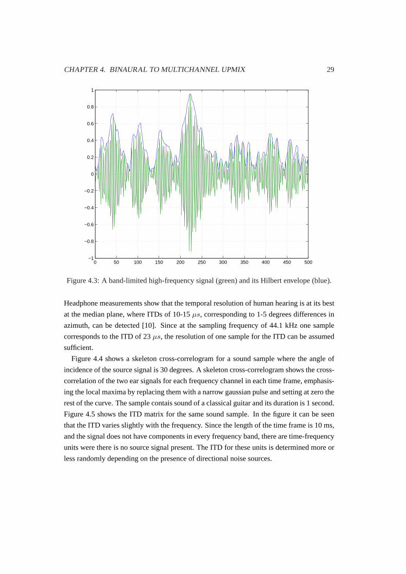
CHAPTER 4. BINAURAL TO MULTICHANNEL UPMIX 29
0 50 100 150 200 250 300 350 400 450 500−1
−0.8
−0.6
−0.4
−0.2
0
0.2
0.4
0.6
0.8
1
Figure 4.3:A band-limited high-frequency signal (green) and its Hilbert envelope (blue).
Headphone measurements show that the temporal resolution of human hearing is at its best
at the median plane, where ITDs of 10-15µs, corresponding to 1-5 degrees differences in
azimuth, can be detected [10]. Since at the sampling frequency of 44.1 kHz one sample
corresponds to the ITD of 23µs, the resolution of one sample for the ITD can be assumed
sufficient.
Figure4.4 shows a skeleton cross-correlogram for a sound sample where the angle of
incidence of the source signal is 30 degrees. A skeleton cross-correlogram shows the cross-
correlation of the two ear signals for each frequency channel in each time frame, emphasis-
ing the local maxima by replacing them with a narrow gaussian pulse and setting at zero the
rest of the curve. The sample contais sound of a classical guitar and its duration is 1 second.
Figure4.5 shows the ITD matrix for the same sound sample. In the figure it can be seen
that the ITD varies slightly with the frequency. Since the length of the time frame is 10 ms,
and the signal does not have components in every frequency band, there are time-frequency
units were there is no source signal present. The ITD for these units is determined more or
less randomly depending on the presence of directional noise sources.
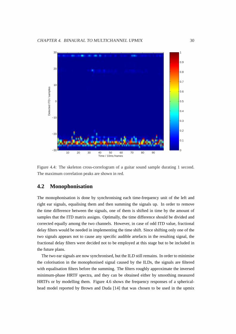
CHAPTER 4. BINAURAL TO MULTICHANNEL UPMIX 30
Time / 10ms frames
Det
ecte
d IT
D /
sam
ples
10 20 30 40 50 60 70 80 90
30
20
10
0
−10
−20
−30 0
0.1
0.2
0.3
0.4
0.5
0.6
0.7
0.8
0.9
1
Figure 4.4:The skeleton cross-correlogram of a guitar sound sample durating 1 second.
The maximum correlation peaks are shown in red.
4.2 Monophonisation
The monophonisation is done by synchronising each time-frequency unit of the left and
right ear signals, equalising them and then summing the signals up. In order to remove
the time difference between the signals, one of them is shifted in time by the amount of
samples that the ITD matrix assigns. Optimally, the time difference should be divided and
corrected equally among the two channels. However, in case of odd ITD value, fractional
delay filters would be needed in implementing the time shift. Since shifting only one of the
two signals appears not to cause any specific audible artefacts in the resulting signal, the
fractional delay filters were decided not to be employed at this stage but to be included in
the future plans.
The two ear signals are now synchronised, but the ILD still remains. In order to minimise
the colorisation in the monophonised signal caused by the ILDs, the signals are filtered
with equalisation filters before the summing. The filters roughly approximate the inversed
minimum-phase HRTF spectra, and they can be obtained either by smoothing measured
HRTFs or by modelling them. Figure4.6 shows the frequency responses of a spherical-
head model reported by Brown and Duda [14] that was chosen to be used in the upmix
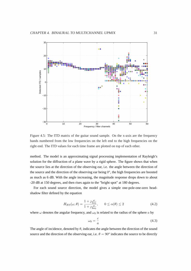
CHAPTER 4. BINAURAL TO MULTICHANNEL UPMIX 31
0 10 20 30 40 50 60−30
−20
−10
0
10
20
30
Frequency / filter channels
Det
ecte
d IT
D /
sam
ples
Figure 4.5:The ITD matrix of the guitar sound sample. On the x-axis are the frequency
bands numbered from the low frequencies on the left end to the high frequencies on the
right end. The ITD values for each time frame are plotted on top of each other.
method. The model is an approximating signal processing implementation of Rayleigh’s
solution for the diffraction of a plane wave by a rigid sphere. The figure shows that when
the source lies at the direction of the observing ear, i.e. the angle between the direction of
the source and the direction of the observing ear being0o, the high frequencies are boosted
as much as 6 dB. With the angle increasing, the magnitude response drops down to about
-20 dB at 150 degrees, and then rises again to the "bright spot" at 180 degrees.
For each sound source direction, the model gives a simple one-pole-one-zero head-
shadow filter defined by the equation
HHS(ω, θ) =1 + ω
2ω0
1 + ω2ω0
, 0 ≤ α(θ) ≤ 2 (4.2)
whereω denotes the angular frequency, andω0 is related to the radius of the spherea by
ω0 =c
a(4.3)
The angle of incidence, denoted byθ, indicates the angle between the direction of the sound
source and the direction of the observing ear, i.e.θ = 90o indicates the source to be directly
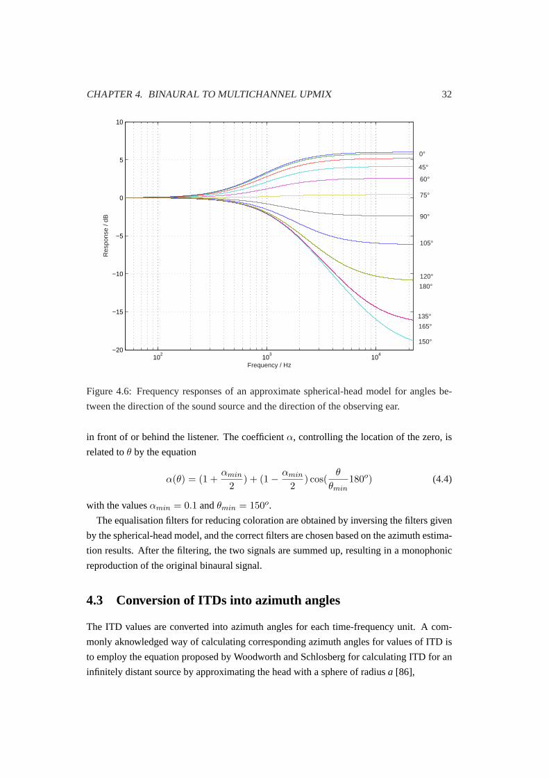
CHAPTER 4. BINAURAL TO MULTICHANNEL UPMIX 32
102
103
104
−20
−15
−10
−5
0
5
10
Frequency / Hz
Res
pons
e / d
B
0°
150°
135°
45°
60°
75°
90°
105°
120°
180°
165°
Figure 4.6:Frequency responses of an approximate spherical-head model for angles be-
tween the direction of the sound source and the direction of the observing ear.
in front of or behind the listener. The coefficientα, controlling the location of the zero, is
related toθ by the equation
α(θ) = (1 +αmin
2) + (1− αmin
2) cos(
θ
θmin180o) (4.4)
with the valuesαmin = 0.1 andθmin = 150o.
The equalisation filters for reducing coloration are obtained by inversing the filters given
by the spherical-head model, and the correct filters are chosen based on the azimuth estima-
tion results. After the filtering, the two signals are summed up, resulting in a monophonic
reproduction of the original binaural signal.
4.3 Conversion of ITDs into azimuth angles
The ITD values are converted into azimuth angles for each time-frequency unit. A com-
monly aknowledged way of calculating corresponding azimuth angles for values of ITD is
to employ the equation proposed by Woodworth and Schlosberg for calculating ITD for an
infinitely distant source by approximating the head with a sphere of radiusa [86],
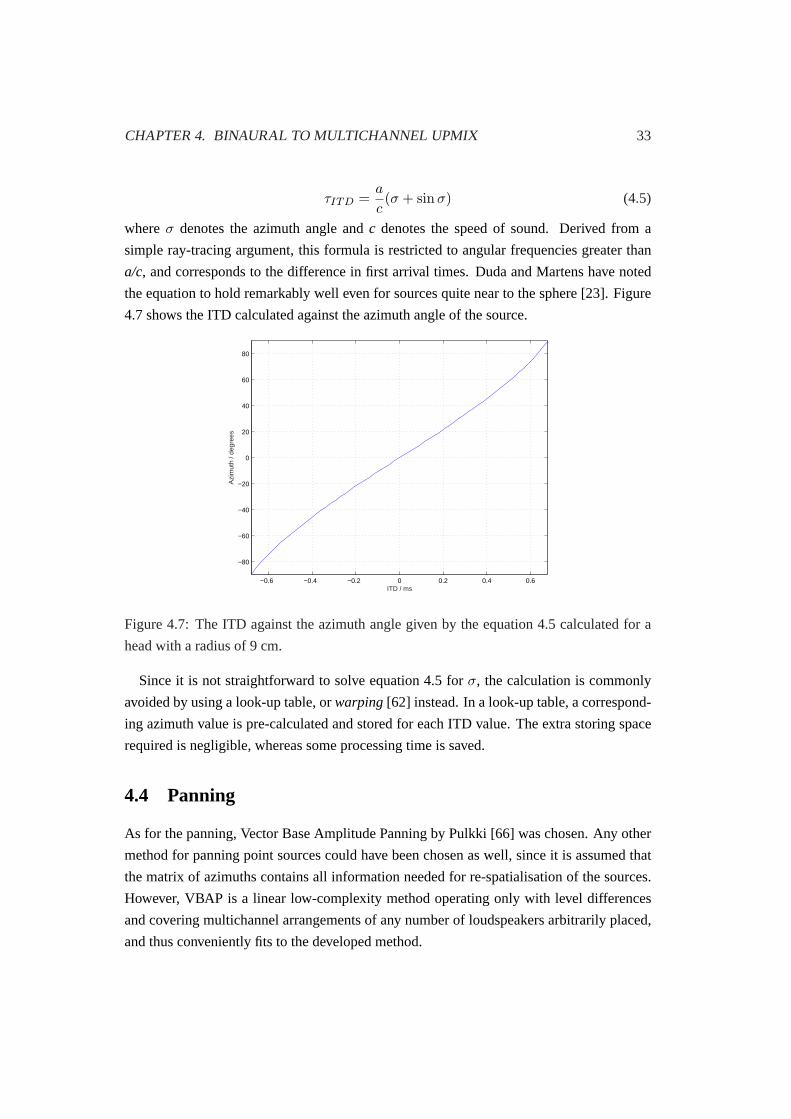
CHAPTER 4. BINAURAL TO MULTICHANNEL UPMIX 33
τITD =a
c(σ + sin σ) (4.5)
whereσ denotes the azimuth angle andc denotes the speed of sound. Derived from a
simple ray-tracing argument, this formula is restricted to angular frequencies greater than
a/c, and corresponds to the difference in first arrival times. Duda and Martens have noted
the equation to hold remarkably well even for sources quite near to the sphere [23]. Figure
4.7shows the ITD calculated against the azimuth angle of the source.
−0.6 −0.4 −0.2 0 0.2 0.4 0.6
−80
−60
−40
−20
0
20
40
60
80
ITD / ms
Azi
mut
h / d
egre
es
Figure 4.7:The ITD against the azimuth angle given by the equation4.5 calculated for a
head with a radius of 9 cm.
Since it is not straightforward to solve equation4.5 for σ, the calculation is commonly
avoided by using a look-up table, orwarping[62] instead. In a look-up table, a correspond-
ing azimuth value is pre-calculated and stored for each ITD value. The extra storing space
required is negligible, whereas some processing time is saved.
4.4 Panning
As for the panning, Vector Base Amplitude Panning by Pulkki [66] was chosen. Any other
method for panning point sources could have been chosen as well, since it is assumed that
the matrix of azimuths contains all information needed for re-spatialisation of the sources.
However, VBAP is a linear low-complexity method operating only with level differences
and covering multichannel arrangements of any number of loudspeakers arbitrarily placed,
and thus conveniently fits to the developed method.
CHAPTER 4. BINAURAL TO MULTICHANNEL UPMIX 34
In VBAP, the panning of the virtual sources in the azimuth dimension is done by using
two adjacent loudspeakers closest to the source location, and adjusting their loudness levels
with a gain factor calculated as described in section 3.3.3. To be able to perform this calcu-
lation, both the angle of incidence of the sound sources, as well as the direction angles of
the loudspeakers in relation to the listening point, are required.
The direction angles of the loudspeakers are assumed to be known at this stage, and so
the gain factors for each time-frequency unit can be calculated from the equation3.1. Each
unit is multiplied by the corresponding gain factor, and the units are then summed along
frequency and interpolated along time. Cross-fading type linear interpolation is used, due
to its fastness and simplicity [83], though more complex interpolation methods should also
be experimented with.
In order to achieve a smoother panning of the spatial signal, the ITD matrix has to be
made more sparse. During the development of the method, it was noted that implementing
the panning with a time-frequency matrix as dense as produced by the azimuth estimation,
causes audible artefacts in the resulting signal. This is believed by the author to be due to the
unavoidable estimation errors causing the loudspeaker gains to fluctuate unnaturally rapidly.
Consequently, in order to smoothen the panning, the azimuth matrix is made more sparse.
Through experimenting, it was found that an adequate size for a time-frequency unit results
from dividing the signal into 30 frequency bands and 100 ms time frames overlapping by
50%. The azimuth values for the sparse matrix are gained by averiging the values of the
denser original matrix. The averiging also corrects some of the estimated ITD values that
have obviously been estimated incorrectly. Figure4.8 shows a sparse version of the ITD
matrix shown in figure4.5.
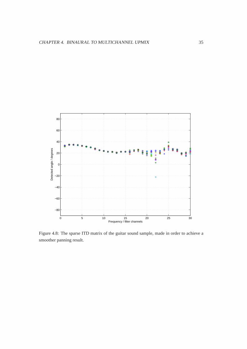
CHAPTER 4. BINAURAL TO MULTICHANNEL UPMIX 35
0 5 10 15 20 25 30
−80
−60
−40
−20
0
20
40
60
80
Frequency / filter channels
Det
ecte
d an
gle
/ deg
rees
Figure 4.8:The sparse ITD matrix of the guitar sound sample, made in order to achieve a
smoother panning result.
Chapter 5
Testing and results
In order to verify the functionality of the binaural to multichannel upmix method developed,
it was tested in a variety of ways. For audio signal processing methods, listening is generally
the most important way of evaluation and troubleshooting. Thus, during the development,
the upmix method has been continuously debugged and evaluated by listening. This part of
the testing is reported in section 5.1.
Measuring and quantifying the performance is in most cases possible and aids in compar-
ing both different versions of the method, as well as the method to other methods, but what
ultimately judges a method is its success in producing the desired auditory sensation. Thus,
the most important means of verification is the listening test reported in section 5.2. The
test was informal and rather small-scale, but the results were promising and gave direction
for future work.
5.1 General testing during the development of the method
A set of sound samples varying from free-field to binaural modelling, introduced in section
5.1.1, were created for testing the method during the development work. Section 5.1.2.
reports the results of testing the method when noise was added in the test samples. Section
5.1.3. discusses the use of different sized auditory filter banks and time frames.
5.1.1 Sound samples
The upmix method was continuously tested with two types of sound samples during the
development. The samples were required to be "easy" enough for the method to process, so
that elementary errors would be rapidly detected. The most primitive sound samples were
produced by duplicating a monophonic signal into two signal channels, and delaying one
of the channels so as to create an Interchannel Time Difference (ICTD). Though this kind
36
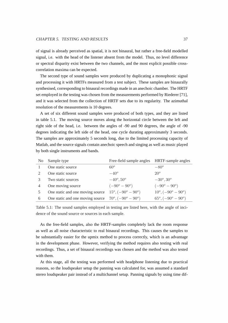
CHAPTER 5. TESTING AND RESULTS 37
of signal is already perceived as spatial, it is not binaural, but rather a free-field modelled
signal, i.e. with the head of the listener absent from the model. Thus, no level difference
or spectral disparity exist between the two channels, and the most explicit possible cross-
correlation maxima can be expected.
The second type of sound samples were produced by duplicating a monophonic signal
and processing it with HRTFs measured from a test subject. These samples are binaurally
synthesised, corresponding to binaural recordings made in an anechoic chamber. The HRTF
set employed in the testing was chosen from the measurements performed by Riederer [71],
and it was selected from the collection of HRTF sets due to its regularity. The azimuthal
resolution of the measurements is 10 degrees.
A set of six different sound samples were produced of both types, and they are listed
in table5.1. The moving source moves along the horizontal circle between the left and
right side of the head, i.e. between the angles of -90 and 90 degrees, the angle of -90
degrees indicating the left side of the head, one cycle durating approximately 3 seconds.
The samples are approximately 5 seconds long, due to the limited processing capacity of
Matlab, and the source signals contain anechoic speech and singing as well as music played
by both single instruments and bands.
No Sample type Free-field sample angles HRTF-sample angles
1 One static source 60o −80o
2 One static source −40o 20o
3 Two static sources −40o, 50o −30o, 30o
4 One moving source (−90o − 90o) (−90o − 90o)5 One static and one moving source15o, (−90o − 90o) 10o, (−90o − 90o)6 One static and one moving source70o, (−90o − 90o) 65o, (−90o − 90o)
Table 5.1:The sound samples employed in testing are listed here, with the angle of inci-
dence of the sound source or sources in each sample.
As the free-field samples, also the HRTF-samples completely lack the room response
as well as all noise characteristic to real binaural recordings. This causes the samples to
be substantially easier for the upmix method to process correctly, which is an advantage
in the development phase. However, verifying the method requires also testing with real
recordings. Thus, a set of binaural recordings was chosen and the method was also tested
with them.
At this stage, all the testing was performed with headphone listening due to practical
reasons, so the loudspeaker setup the panning was calculated for, was assumed a standard
stereo loudspeaker pair instead of a multichannel setup. Panning signals by using time dif-
CHAPTER 5. TESTING AND RESULTS 38
ference or level difference alternatively do not generally produce exactly similar sounding
results, so this kind of testing is quite rough. Nonetheless, the test revealed that the sources
are kept well segregated and compact by the processing, and they appear clearly in their
original directions after the processing. When listening to the samples at the stage of the
process where they are monophonised, they sound remarkably similar to the corresponding
original monophonic samples. This implies success in removing the ITD from the binaural
signal.
The ITD matrices produced by the method for each free-field sample and HRTF-sample
were evaluated in order to rate the erroneousness of the azimuth estimation. It was found,
that 90% of the estimates fall within error marginal of approximately 5% of the total range
of values, while the rest of the estimates may introduce error of up to 100% of the range.
Nonetheless, it appears that the erroneousness is not audible, but rather ends up masked
within the signal.
When the method was tested with the real binaural recordings, the results were, as ex-
pected, not as good as for the anechoic sound samples. However, the method performed
well regarding the fact that no processing was done in order to handle the echoes or noise.
The error marginal for the azimuth estimation increased to approximately 10% of the total
ITD range, but the upmixed samples still sounded rather clear.
5.1.2 Background noise test
The following step of testing was to add noise in the sound samples. Since real binaural
recordings are assumed to contain background noise, only the free-field samples and HRTF-
samples were tested with added noise. Four noise levels were tested, which were -6 dB, 0
dB, 6 dB and 12 dB in relation to the average signal level. First, uncorrelated pink noise
was added in the samples, pink noise signifying noise that has even distribution of power
when the frequency is mapped in a logarithmic scale. The pink noise was found to have no
effect on the azimuth estimation at any test level. This could be expected since uncorrelated
noise does not cause any disturbance in the cross-correlation calculation.
Next, binaurally recorded background noise was added in the samples. Three different
noise recordings from a collection recorded by Peltonenet al. [64] were used, containing
sound environments recorded in a café, in an office and in a shop. The binaural noise was
expected to degrade the performance of the azimuth estimation, since it causes additional
and unwanted directional sources to appear and disturb the cross-correlation calculation.
However, the results were better than expected. Error in the azimuth estimation increased
slightly, but it did not become audible. It appears that the possible additional error occurs
in the direction of the background noise sources and is thus masked by the noise itself.
CHAPTER 5. TESTING AND RESULTS 39
5.1.3 The effect of the auditory filter bank and time frame size
Though the filter channel and time frame sizes are mostly restricted by the theory of the
human hearing, especially in the azimuth estimation part, some variations were tested dur-
ing the development of the method. According to the time-frequency theory, if the units
are small-sized enough, each unit can be assumed to be perceptually dominated by a single
sound source. Frequency-wise, the assumption is based on the theory of the critical band,
which defines the smallest band of frequencies which activate the same part of the basilar
membrane at each center frequency. Time-wise, the maximum frame length is defined by
the masking phenomenon, i.e. minor sources being temporally masked by the dominant
source within its immediate range. On the other hand, if the unit size is reduced too much,
there are not enough samples left per unit, which causes the calculation accuracy to suffer.
For azimuth estimation, previous research indicates the suitable unit size to be about 60
logarithmically equal frequency bands between 200 Hz and 22050 Hz with time frames of
20 ms. For the panning, however, this small units seem to be too short, causing unnaturally
rapid fluctuation of the gain factors. Through listening, suitable unit size for panning was
found to be approximately double sized frequency bands compared to the filter bank used
by the azimuth estimation, with time frames of approximately 100 ms. Further increasing
of the unit size begins to affect the accuracy of the panning, the moving speed of some real
sources exceeding the performance of the interpolation.
5.2 Listening test
In order to supplement the general testing and verify the correct functioning of the upmix
method, a listening test was performed. The test setup is described in section 5.2.1 and the
results are discussed in section 5.2.2. Section 5.2.3 presents some general observations of
the listening test.
5.2.1 Test setup
The listening test was performed in a standard listening room, where earplugs and a 5.0
loudspeaker setup were used for playback. In the test, nine multichannel sound samples
were compared to their binaural counterparts. The samples were approximately 5 seconds
long and contained anechoic speech and singing as well as music played by both single
instruments and bands. The binaural samples were made by convolving monophonic sound
samples with measured HRIRs, and the multichannel samples were produced by upmix-
ing the binaural samples with the developed upmix method. Table5.2 categorises the test
samples.
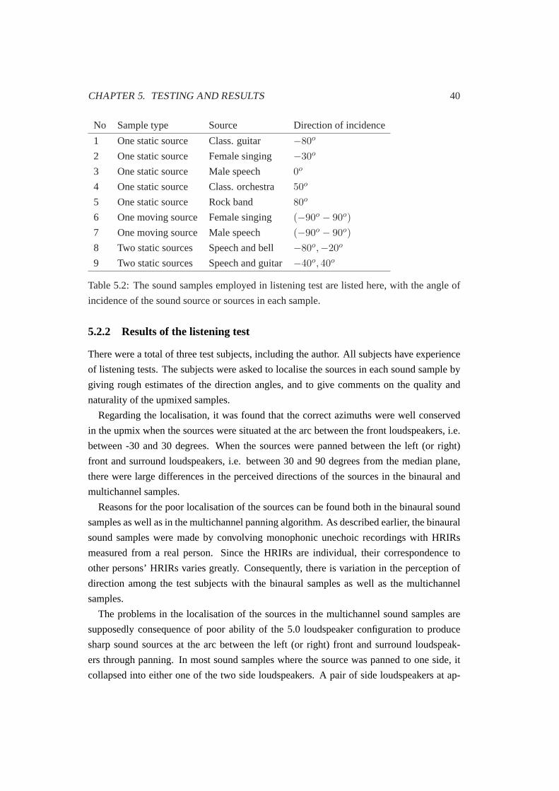
CHAPTER 5. TESTING AND RESULTS 40
No Sample type Source Direction of incidence
1 One static source Class. guitar −80o
2 One static source Female singing −30o
3 One static source Male speech 0o
4 One static source Class. orchestra50o
5 One static source Rock band 80o
6 One moving source Female singing (−90o − 90o)7 One moving source Male speech (−90o − 90o)8 Two static sources Speech and bell −80o,−20o
9 Two static sources Speech and guitar−40o, 40o
Table 5.2:The sound samples employed in listening test are listed here, with the angle of
incidence of the sound source or sources in each sample.
5.2.2 Results of the listening test
There were a total of three test subjects, including the author. All subjects have experience
of listening tests. The subjects were asked to localise the sources in each sound sample by
giving rough estimates of the direction angles, and to give comments on the quality and
naturality of the upmixed samples.
Regarding the localisation, it was found that the correct azimuths were well conserved
in the upmix when the sources were situated at the arc between the front loudspeakers, i.e.
between -30 and 30 degrees. When the sources were panned between the left (or right)
front and surround loudspeakers, i.e. between 30 and 90 degrees from the median plane,
there were large differences in the perceived directions of the sources in the binaural and
multichannel samples.
Reasons for the poor localisation of the sources can be found both in the binaural sound
samples as well as in the multichannel panning algorithm. As described earlier, the binaural
sound samples were made by convolving monophonic unechoic recordings with HRIRs
measured from a real person. Since the HRIRs are individual, their correspondence to
other persons’ HRIRs varies greatly. Consequently, there is variation in the perception of
direction among the test subjects with the binaural samples as well as the multichannel
samples.
The problems in the localisation of the sources in the multichannel sound samples are
supposedly consequence of poor ability of the 5.0 loudspeaker configuration to produce
sharp sound sources at the arc between the left (or right) front and surround loudspeak-
ers through panning. In most sound samples where the source was panned to one side, it
collapsed into either one of the two side loudspeakers. A pair of side loudspeakers at ap-
CHAPTER 5. TESTING AND RESULTS 41
proximately 90 degrees angles would thus be required in order to pan the sources correctly.
On the sound quality of the upmixed samples, it was found that the quality of the samples
containing sounds of single or multiple musical instruments did not deteriorate significantly,
whereas the quality of the samples containing human voice deteriorated noticeably. The test
subjects described some of the deteriorated samples as sounding "metallic" and others noisy
or "burbling". The reason for the deterioration of the quality is under investigation.
5.2.3 General observations
It is probable that the most severe weakness of the upmix method at this stage is its poor
performance in the presence of room response in the binaural signal. It would also be
beneficial for the method to be able to "concentrate" on the strong and clear sound sources,
that can be assumed the interesting ones, and depress the background noise in order to
transmit the main sources as clearly as possible. The future plans for the development of
the method are discussed in the following chapter.
Chapter 6
Conclusions and future work
In this thesis, a method was described for upmixing binaural audio into multichannel format
while preserving the information for correct spatial sensation. The method is motivated by
its application possibilities in telepresence and teleconferencing technologies as well as
in audio coding, to mention some, and its development is given reasons by the existing
gap in the upmix and downmix techniques among audio playback formats. This chapter
will summarise the main results of this thesis. The method, as well as its advantages and
limitations, are discussed in section 6.1. Ideas and plans for improving the method are
presented in section 6.2.
6.1 Conclusions and discussion
In its simplest, the binaural to multichannel upmix method can be thought of as a conversion
of Interaural Time Difference (ITD) into InterChannel Level Difference (ICLD). A good
deal of the method bases on methods developed by Palomäkiet al. [62] and Pulkki [66].
The azimuth estimation is done by dividing the signal into time-frequency units with a
cochlear filter bank and 10 ms time frames, and using in the analysis ITD information only.
The ITD is then removed from the signal, and the synchronised ear channel signals are
equalised and summed, resulting in a monophonised signal. The ITD information is stored
in a matrix, potentially transmitted along with the monophonic signal.
In the panning phase, practically any desired multichannel panning method can be em-
ployed. The information for the spatial placing of the sound can be derived from the ITD
matrix by converting the ITD of each time-frequency unit into the corresponding angle of
incidence of sound. In this thesis, the Vector Base Amplitude Panning (VBAP) was used as
the panning method, due to its low complexity as well as the ability to produce sharp vir-
tual sources. The gain factor for each loudspeaker per each time-frequency unit are derived
42
CHAPTER 6. CONCLUSIONS AND FUTURE WORK 43
from the angles of incidence calculated from the ITD matrix.
The main limitation of the method, causing it to fail the definition of a fully three-
dimensional system, is that from binaural signal, with the excisting techniques only the
azimuths of the front (or back) half plane can be unambiguously detected. Due to the
cone of confusion, neither elevations nor the back or front directions can be distinguished.
Adding the use of ILD cues in the estimation does not bring enough information to solve
the ambiguities. Thus, all sound sources have to be assumed to lie on the frontal azimuthal
half circle of the listener’s head. On the other hand, the most probable playback system
for the upmixed multichannel audio is the de facto standard 5.1 home theater loudspeaker
system, where the sharpest resolution for producing virtual sources lies in the frontal direc-
tions, and no loudspeakers for reproducing elevated sources are available anyway. Further-
more, regarding application areas, such as telepresence or teleconferencing, the "interest-
ing" sources of sound can be assumed to lie in the frontal plane of the listener, where he/she
can see them. Consequently, the lack of full 3-D coverage of the acoustic environment is
not as great a fault of the method as first deduced.
Another limitation of the upmix method is that the coloration caused to the binaurally
recorded sound by the head shadow cannot be fully removed in the monophonisation. Thus,
the quality of upmixed multichannel sound will not be as good as the quality of a corre-
sponding multichannel recording. The coloration can be reduced to some point by using
equalisation filters roughly following the measured ILDs for different angles of incidence.
The remaining coloration will have to be hoped to loose significance when merging with
the room effect of the listening space added to the upmixed multichannel sound.
A matter for a profound consideration on the upmix method is the question wheather it
would be more sensible to carry out the upmix process through stereophonising, instead of
monophonising, of the binaural signal. Employing of stereophonisation would be favoured
by the existance of high quality binaural to stereo as well as stereo to multichannel con-
version techniques, and the prospect of losing less information in the upmix. This might
improve the quality of the processed multichannel audio. On the other hand, the advance
of the monophonisation is that less storing and transmission capacity is required when the
downmix from binaural to monophonic signal and the upmix from monophonic to multi-
channel signal are desired to be performed separately. In any case, this confrontation should
be thoroughly studied.
6.2 Future work
The development work on the upmix method described here is only at its beginning, and
thus the list of possible improvements is a long one. There are several ways to improve
CHAPTER 6. CONCLUSIONS AND FUTURE WORK 44
the azimuth estimation in the method. To perform the conversion of ITDs to angles of in-
cidence of the sound more accurately, a better model of the human head is required. The
model should take into account both the asymmetry of the head, as well as the frequency de-
pendence of the ITD. A sufficiently accurate model might be the adaptable ellipsoidal head
model introduced by Dudaet al. [22]. The angles of incidence could either be calculated
from the head model for each time-frequency unit in real-time, or the corresponding values
for each possible ITD value could be stored in a look-up table beforehand. The decision
depends on the performance requirements for the implementation.
The performance of the azimuth estimation in the presence of room reflections and re-
verberation can be substantially improved by adding precedence effect modelling to the
method. The success of implementing precedence effect modelling to azimuth estimation
is proven by the speech segregation research done by Palomäkiet al. [62]. Also the addition
of ILD cues in the estimation should be considered another time, when the method evolves
further.
Regarding the quality of the upmixed sound, the most significant improvement would
very likely be the implementation of the extraction of ambience noise from the original bin-
aural signal before the azimuth analysis. Ambience extraction has been profoundly studied
in the stereo to multichannel upmix by Avendano and Jot [5], and in the general source lo-
calisation by Faller and Merimaa [25]. Also better equalisation of the binaural signal before
monophonising it, in order to reduce the coloration caused by the ILD, would improve the
sound quality considerably. Fractional delay filters could be used in the synchronisation of
the left and right ear signals, resulting in a more accurate synchronisation [48]. The pos-
sibilities for replacing the linear interpolation, used in the panning of the time-frequency
units, with a more advanced interpolation algorithm should be studied.
In order to have the upmix method properly testable, it should as soon as possible be
implemented in an environment capable of real-time processing. The algorithm should also
be optimised, so as to find out the overall requirements for processing capacity.
Bibliography
[1] V. R. Algazi, R. O. Duda, D. M. Thompson, and C. Avendano. The CIPIC HRTF
database. InProceedings of the IEEE Workshop on Applications of Signal Processing
to Audio and Electroacoustics, pages 99–102, New Paltz, USA, October 21-24 2001.
[2] J. B. Allen and D. A. Berkley. Image method for efficiently simulating small-room
acoustics.Journal of the Acoustical Society of America, 65(4):943–950, 1979.
[3] C. Avendano and J.-M. Jot. Ambience extraction and synthesis from stereo signals
for multichannel audio upmix. InProceedings of the IEEE International Conference
on Acoustics, Speech and Signal Processing, volume 2, pages 1957–1960, Orlando,
USA, May 13-17 2002.
[4] C. Avendano and J.-M. Jot. Frequency domain techniques for stereo to multichannel
upmix. InProceedings of the Audio Engineering Society 22nd International Confer-
ence, pages 121–130, Espoo, Finland, June 15-17 2002.
[5] C. Avendano and J.-M. Jot. A frequency-domain approach to multichannel upmix.
Journal of the Audio Engineering Society, 52(7/8):740–749, 2004.
[6] D. W. Batteau. The role of the pinna in human localization.Proceedings of the Royal
Society London, 168 (series B):158–180, 1967.
[7] A. J. Berkhout. A holographic approach to acoustic control.Journal of the Audio
Engineering Society, 36(12):977–995, 1988.
[8] A. J. Berkhout, D. de Vries, and P. Vogel. Acoustic control by wave field synthesis.
Journal of the Acoustical Society of America, 93(5):2764–2778, 1993.
[9] L. R. Bernstein and C. Trahiotis. Transposed stimuli reveal similar underlying sen-
sitivity to interaural timing information at high and low frequencies.Journal of the
Acoustical Society of America, 109(5):2485–2485, 2001.
45
BIBLIOGRAPHY 46
[10] J. Blauert.Spatial Hearing: The Psychophysics of Human Sound Localization. MIT
Press, Cambridge, MA, 1st edition, 1997.
[11] A. D. Blumlein. U.K. Patent 394,325, 1931. Reprinted in Stereophonic Techniques
(AES, New York, 1986), 1931.
[12] J. Breebaart, S. van de Par, A. Kohlrausch, and E. Schuijers. High-quality parametric
spatial audio coding at low bitrates. InProceedings of the Audio Engineering Society
116th Convention, Preprint 6072, Berlin, Germany, May 8-11 2004.
[13] A. S. Bregman.Auditory Scene Analysis. MIT Press, Cambridge, MA, 1st edition,
1990.
[14] C. P. Brown and R. O. Duda. A structural model for binaural sound synthesis.IEEE
Transactions on Speech and Audio Processing, 6(5):476–488, September 1998.
[15] S. Cavaco and J. Hallam. A biologically plausible acoustic azimuth estimation system.
In H. G. Okuno and F. Klassner, editors,Working notes of the 3rd IJCAI Workshop on
Computational Auditory Scene Analysis, Stockholm, Sweden, August 1 1999.
[16] E. C. Cherry. Some experiments on the recognition of speech with one and with two
ears.Journal of the Acoustical Society of America, 25(5):975–979, 1953.
[17] F. Christensen, C. B. Jensen, and H. Møller. The design of VALDEMAR: An artificial
head for binaural recording purposes. InProceedings of the Audio Engineering Society
109th Convention, Preprint 5253, Los Angeles, USA, September 22-25 2000.
[18] M. Cohen, S. Aoki, and N. Koizumi. Augmented audio reality: Telepresence/VR
hybrid acoustic environments. InProceedings of the 2nd IEEE International Work-
shop on Robot and Human Communication, pages 361–364, Tokyo, Japan, November
1993.
[19] P. Damaske. Head-related two-channel stereophony with loudspeaker reproduction.
Journal of the Acoustical Society of America, 50(4):1109–1115, 1971.
[20] C. J. Darwin and R. P. Carlyon. Auditory grouping. In B. C. J. Moore, editor,Hearing,
6, pages 387–424. Academic, London, 1995.
[21] Dolby Headphone. http://www.dolby.com/consumer/technology/headphone.html.
Dolby Laboratories, Inc., 2005. Referred June 6, 2005.
[22] R. O. Duda, C. Avendano, and R. Algazi. An adaptable ellipsoidal head model for the
interaural time difference. InProceedings of the IEEE International Conference on
BIBLIOGRAPHY 47
Acoustics, Speech and Signal Processing, volume 2, pages 965–968, Phoenix, USA,
March 15-19 1999.
[23] R. O. Duda and W. L. Martens. Range dependence of the response of a spherical head
model.Journal of the Acoustical Society of America, 104(5):3048–3058, 1998.
[24] C. Faller and F. Baumgarte. Binaural cue coding applied to stereo and multichannel
audio compression. InProceedings of the Audio Engineering Society 112th Conven-
tion, Preprint 5574, Munich, Germany, May 10-13 2002.
[25] C. Faller and J. Merimaa. Source localization in complex listening situations: Selec-
tion of binaural cues based on interaural coherence.Journal of the Acoustical Society
of America, 116(5):3075–3089, 2004.
[26] K. Farrah. The Soundfield microphone.Wireless World, 85:48–50, 99–102, January
1979.
[27] R. K. Furness. Ambisonics - an overview. InProceedings of the Audio Engineering
Society 8th International Conference, pages 181–190, Washington, USA, May 3-6
1990.
[28] W. G. Gardner and K. Martin. HRTF measurements of a KEMAR dummy-head mi-
crophone. Technical Report 280, MIT - Media Lab Perceptual Computing Group,
1994.
[29] M. A. Gerzon. Design of Ambisonic decoders for multispeaker surround sound. In
Proceedings of the Audio Engineering Society 58th Convention, no preprint, New
York, USA, November 4 1977.
[30] M. A. Gerzon. Signal processing for simulating realistic stereo images. InProceedings
of the Audio Engineering Society 93rd Convention, Preprint 3423, San Francisco,
USA, October 1-4 1992.
[31] D. Griesinger. Equalization and spatial equalization of dummy-head recordings for
loudspeaker reproduction.Journal of the Audio Engineering Society, 37(1/2):20–29,
1989.
[32] D. Hammershøi. Fundamental aspects of the binaural recording and synthesis tech-
niques. InProceedings of the Audio Engineering Society 100th Convention, Preprint
4155, Copenhagen, Denmark, May 11-14 1996.
BIBLIOGRAPHY 48
[33] W. M. Hartmann. Listening in a room and the precedence effect. In R. H. Gilkey and
T. R. Anderson, editors,Binaural and Spatial Hearing in Real and Virtual Environ-
ments, pages 191–210. L. Erlbaum Associates, 1st edition, 1996.
[34] J. Herre, K. Brandenburg, and D. Lederer. Intensity stereo coding. InProceedings
of the Audio Engineering Society 96th Convention, Preprint 3799, Amsterdam, The
Netherlands, February 26-March 1 1994.
[35] U. Horbach and M. M. Boone. Future transmission and rendering formats for multi-
channel sound. InProceedings of the Audio Engineering Society 16th International
Conference, pages 409–418, Rovaniemi, Finland, April 10-12 1999.
[36] A. Härmä and C. Faller. Spatial decomposition of time-frequency regions: subbands
or sinusoids. InProceedings of the Audio Engineering Society 116th Convention,
Preprint 6061, Berlin, Germany, May 8-11 2004.
[37] A. Härmä, J. Jakka, M. Tikander, M. Karjalainen, T. Lokki, J. Hiipakka, and G. Lorho.
Augmented reality audio for mobile and wearable appliances.Journal of the Audio
Engineering Society, 52(6):618–639, 2004.
[38] J. Huopaniemi, N. Zacharov, and M. Karjalainen. Objective and subjective evalua-
tion of head-related transfer function filter design.Journal of the Audio Engineering
Society, 47(4):218–239, 1999.
[39] L. A. Jeffress. A place theory of sound localization.Journal of Comparative and
Physiological Psychology, 61:468–486, 1948.
[40] J. D. Johnston and A. J. Ferreira. Sum-difference stereo transform coding. InProceed-
ings of the IEEE International Conference on Acoustics, Speech and Signal Process-
ing, pages 569–572, San Francisco, USA, March 23-26 1992.
[41] J.-M. Jot and V. Larcher. Approaches to binaural synthesis. InProceedings of the
Audio Engineering Society 105th Convention, Preprint 4861, San Francisco, USA,
September 26-29 1998.
[42] J.-M. Jot, V. Larcher, and J.-M. Pernaux. A comparative study of 3-D audio encod-
ing and rendering techniques. InProceedings of the Audio Engineering Society 16th
International Conference, pages 281–300, Rovaniemi, Finland, April 10-12 1999.
[43] J. Kawaura, Y. Suzuki, F. Asano, and T. Sone. Sound localization in headphone re-
production by simulating transfer functions from the sound source to the external ear.
Journal of the Acoustical Society of Japan, (E)12:203–216, 1991.
BIBLIOGRAPHY 49
[44] G. S. Kendall, W. L. Martens, D. J. Freed, M. D. Ludwig, and R. Karstens. Image-
model reverberation from recirculating delays. InProceedings of the Audio Engi-
neering Society 81st Convention, Preprint 2408, Los Angeles, USA, November 12-16
1986.
[45] G. S. Kendall, W. L. Martens, and M. D. Wilde. A spatial sound processor for loud-
speaker and headphone reproduction. InProceedings of the Audio Engineering Society
8th International Conference, pages 209–221, Washington, USA, May 3-6 1990.
[46] M. Kleiner, B. Dalenbäck, and P. Svensson. Auralization - an overview.Journal of
the Audio Engineering Society, 41(11):861–875, 1993.
[47] K. Kotorynski. Digital binaural/stereo conversion and crosstalk cancelling. InPro-
ceedings of the Audio Engineering Society 89th Convention, Preprint 2949, Los An-
geles, USA, September 21-25 1990.
[48] T. I. Laakso, V. Välimäki, M. Karjalainen, and U. K. Laine. Splitting the unit delay.
IEEE Signal Processing Magazine, 13(1):30–61, January 1996.
[49] C. Lim and R. O. Duda. Estimating the azimuth and elevation of a sound source from
the output of a cochlear model. InProceedings of the IEEE 28th Asilomar Conference
on Signals, Systems and Computers, Asilomar, USA, October 1994.
[50] S. P. Lipshitz. Stereo microphone techniques: Are the purists wrong?Journal of the
Audio Engineering Society, 34(9):716–744, 1986.
[51] E. A. MacPherson. A computer model of binaural localization for stereo imaging
measurement.Journal of the Audio Engineering Society, 39(9):604–622, 1991.
[52] K. D. Martin. Echo suppression in a computational model of the precedence effect. In
Proceedings of the IEEE Workshop on Applications of Signal Processing to Acoustics
and Audio, New Paltz, USA, October 19-22 1997.
[53] D. McFadden and E. G. Pasanen. Lateralization at high frequencies based on interaural
time differences.Journal of the Acoustical Society of America, 59(3):634–639, 1976.
[54] M. Miller. The history of surround sound.
http://www.quepublishing.com/articles/article.asp?p=337317, September 2004.
Referred June 6, 2005.
[55] H. Møller. Reproduction of artificial-head recordings through loudspeakers.Journal
of the Audio Engineering Society, 37(1/2):30–33, 1989.
BIBLIOGRAPHY 50
[56] H. Møller, C. B. Jensen, D. Hammershøi, and M. F. Sørensen. Evaluation of artifi-
cial heads in listening test. InProceedings of the Audio Engineering Society 102nd
Convention, Preprint 4404, Munich, Germany, March 22-25 1997.
[57] H. Møller, M. F. Sørensen, D. Hammershøi, and C. B. Jensen. Head-related transfer
functions of human subjects.Journal of the Audio Engineering Society, 43(5):300–
321, 1995.
[58] B. C. J. Moore.An Introduction to the Psychology of Hearing. Academic Press, San
Diego, USA, 5th edition, 2003.
[59] B. C. J. Moore, R. W. Peters, and B. R. Glasberg. Auditory filter shapes at low center
frequencies.Journal of the Acoustical Society of America, 88(1):132–140, 1990.
[60] A. V. Oppenheim and R. W. Schafer.Discrete-Time Signal Processing. Prentice Hall,
E.Cliffs, 1989.
[61] R. Orban. A rational technique for synthesizing pseudo-stereo from monophonic
sources.Journal of the Audio Engineering Society, 18(2):157–164, 1970.
[62] K. Palomäki, G.J. Brown, and D.A. Wang. A binaural processor for missing data
speech recognition in the presence of noise and small-room reverberation.Elsevier
Speech Communication, 43:361–378, 2004.
[63] R. D. Patterson, I. Nimmo-Smith, J. Holdsworth, and P. Rice. An efficient auditory
filterbank based on the gammatone function. Technical Report 2341, Applied Psy-
chology Unit, Cambridge, 1988.
[64] V. Peltonen, J. Tuomi, A. Klapuri, J. Huopaniemi, and T. Sorsa. Computational au-
ditory scene recognition. InProceedings of the IEEE International Conference on
Acoustics, Speech and Signal Processing, pages 1941–1944, Orlando, USA, May 13-
17 2002.
[65] M. W. Pocock. A computer model of binaural localization. InProceedings of the
Audio Engineering Society 72nd Convention, Preprint 1951, 30, pages 951–952, Ana-
heim, USA, October 23-27 1982.
[66] V. Pulkki. Virtual sound source positioning using vector base amplitude panning.
Journal of the Audio Engineering Society, 45(6):456–466, 1997.
[67] V. Pulkki, J. Merimaa, and T. Lokki. Multichannel reproduction of measured room
responses. InProceedings of the 18th International Congress on Acoustics, pages
1273–1276, Kyoto, Japan, April 4-9 2004.
BIBLIOGRAPHY 51
[68] V. Pulkki, J. Merimaa, and T. Lokki. Reproduction of reverberation with spatial im-
pulse response rendering. InProceedings of the Audio Engineering Society 116th
Convention, Preprint 6057, Berlin, Germany, May 8-11 2004.
[69] G. Richter. BAP Binaural audio processor. InProceedings of the Audio Engineering
Society 92nd Convention, Preprint 3323, Vienna, Austria, March 24-27 1992.
[70] K. A. J. Riederer. Repeatability analysis of head-related transfer function measure-
ments. InProceedings of the Audio Engineering Society 105th Convention, Preprint
4846, San Francisco, USA, September 26-29 1998.
[71] K.J. Riederer. Head-related transfer function measurements. Master’s thesis, Helsinki
University of Technology, 1998.
[72] N. Roman, D. Wang, and G. J. Brown. Speech segregation based on sound localiza-
tion. Journal of the Acoustical Society of America, 114(4):2236–2252, 2003.
[73] R. Sadek and C. Kyriakis. A novel multichannel panning method for standard and
arbitrary loudspeaker configurations. InProceedings of the Audio Engineering Society
117th Convention, Preprint 6263, San Francisco, USA, October 28-31 2004.
[74] M. R. Schroeder. An artificial stereophonic effect obtained from a single audio signal.
Journal of the Audio Engineering Society, 6(2):74–79, 1958.
[75] E. Schuijers, W. Oomen, B. den Brinker, and J. Breebaart. Advances in parametric
coding for high-quality audio. InProceedings of the Audio Engineering Society 114th
Convention, Preprint 5852, Amsterdam, The Netherlands, March 22-25 2003.
[76] M. Slaney. An efficient implementation of the patterson - Holdsworth auditory filter
bank. Technical Report 35, Apple Computer, Inc., 1993.
[77] M. Slaney. Auditory tool box. Technical Report 010, Interval Research Corporation,
1998.
[78] Lord Rayleigh (J.W. Strutt). On our perception of sound direction.Philosophical
Magazine, 13:214–232, 1907.
[79] G. Theile. On the performance of two-channel and multi-channel stereophony. In
Proceedings of the Audio Engineering Society 88th Convention, Preprint 2887, Mon-
treaux, Canada, March 13-16 1990.
[80] M. V. Thomas. Improving the stereo headphone sound image.Journal of the Audio
Engineering Society, 25(7/8):474–478, 1977.
BIBLIOGRAPHY 52
[81] H. Viste and G. Evangelista. On the use of spatial cues to improve binaural source sep-
aration. InProceedings of the 6th International Conference on Digital Audio Effects,
London, UK, September 8-11 2003.
[82] H. Wallach. On sound localization.Journal of the Acoustical Society of America,
10:270–274, 1949.
[83] E. M. Wenzel and S. H. Foster. Perceptual consequences of interpolating head-related
transfer functions during spatial synthesis. InProceedings of the IEEE Workshop on
Applications of Signal Processing to Audio and Acoustics, pages 102–105, New Paltz,
USA, October 17-20 1993.
[84] F. L. Wightman and D. J. Kistler. The dominant role of low-frequency interaural
time differences in sound localization.Journal of the Acoustical Society of America,
91(3):1648–1661, 1992.
[85] F. L. Wightman and D. J. Kistler. Factors affecting relative importance of sound lo-
calization cues. InConference on Binaural and Spatial Hearing, Dayton, OH, USA,
September 9-12 1993.
[86] R. S. Woodworth and G. Schlosberg.Experimental Psychology. Holt Rinehard and
Winston, NY, 1962.
[87] T. C. T. Yin and J. C. K. Chan. Interaural time sensitivity in medial superior olive of
cat. Journal of Neurophysiology, 64:465–488, 1990.
[88] P. M. Zurek. The precedence effect and its possible role in the avoidance of interaural
ambiguities.Journal of the Acoustical Society of America, 67(3):952–964, 1980.
[89] E. Zwicker and H. Fastl.Psychoacoustics: Facts and Models. Springer-Verlag, Hei-
delberg, Germany, 1st edition, 1990.