Intensity Discrimination and Binaural...

Technical University of Denmark

Intensity Discrimination and BinauralInteraction

2nd semester project

DTU Electrical Engineering

Acoustic Technology

Spring semester 2008

Group 5

Troels Schmidt Lindgreen – s073081David Pelegrin Garcia – s070610

Eleftheria Georganti – s073203

Instructor

Sebastien Santurette

DTU Electrical Engineering

Ørsteds Plads, Building 348

2800 Lyngby

Denmark

Telephone +45 4525 3800

http://www.elektro.dtu.dk

Technical University of Denmark

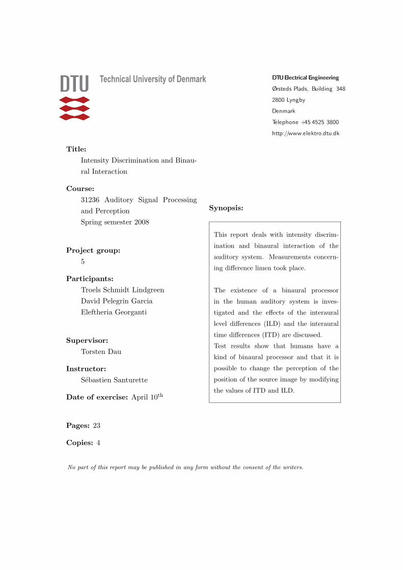
Title:

Intensity Discrimination and Binau-ral Interaction

Course:

31236 Auditory Signal Processingand PerceptionSpring semester 2008

Project group:

5

Participants:

Troels Schmidt LindgreenDavid Pelegrin GarciaEleftheria Georganti

Supervisor:

Torsten Dau

Instructor:

Sebastien Santurette

Date of exercise: April 10th

Pages: 23

Copies: 4

Synopsis:

This report deals with intensity discrim-

ination and binaural interaction of the

auditory system. Measurements concern-

ing difference limen took place.

The existence of a binaural processor

in the human auditory system is inves-

tigated and the effects of the interaural

level differences (ILD) and the interaural

time differences (ITD) are discussed.

Test results show that humans have a

kind of binaural processor and that it is

possible to change the perception of the

position of the source image by modifying

the values of ITD and ILD.

No part of this report may be published in any form without the consent of the writers.

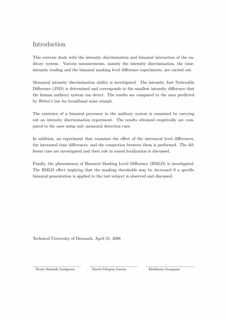
Introduction

This exercise deals with the intensity discrimination and binaural interaction of the au-ditory system. Various measurements, namely the intensity discrimination, the time-intensity trading and the binaural masking level difference experiments, are carried out.

Monaural intensity discrimination ability is investigated. The intensity Just NoticeableDifference (JND) is determined and corresponds to the smallest intensity difference thatthe human auditory system can detect. The results are compared to the ones predictedby Weber’s law for broadband noise stimuli.

The existence of a binaural processor in the auditory system is examined by carryingout an intensity discrimination experiment. The results obtained empirically are com-pared to the ones using only monaural detection cues.

In addition, an experiment that examines the effect of the interaural level differences,the interaural time differences, and the connection between them is performed. The dif-ferent cues are investigated and their role in sound localization is discussed.

Finally, the phenomenon of Binaural Masking Level Difference (BMLD) is investigated.The BMLD effect implying that the masking thresholds may be decreased if a specificbinaural presentation is applied to the test subject is observed and discussed.

Technical University of Denmark, April 21, 2008

Troels Schmidt Lindgreen David Pelegrin Garcia Eleftheria Georganti

Contents

1 Theory 1

1.1 Intensity discrimination . . . . . . . . . . . . . . . . . . . . . . . . . . . . . 11.2 Just noticeable interaural level difference . . . . . . . . . . . . . . . . . . . . 21.3 Interaural time difference . . . . . . . . . . . . . . . . . . . . . . . . . . . . 31.4 Time-intensity trading . . . . . . . . . . . . . . . . . . . . . . . . . . . . . . 41.5 Binaural masking level difference (BMLD) . . . . . . . . . . . . . . . . . . . 5

2 Results 9

2.1 Intensity discrimination . . . . . . . . . . . . . . . . . . . . . . . . . . . . . 92.2 Time-intensity trading . . . . . . . . . . . . . . . . . . . . . . . . . . . . . . 112.3 Binaural Masking Level Difference . . . . . . . . . . . . . . . . . . . . . . . 13

3 Discussion 17

3.1 Interaural level discrimination . . . . . . . . . . . . . . . . . . . . . . . . . . 173.2 Time-intensity trading . . . . . . . . . . . . . . . . . . . . . . . . . . . . . . 173.3 Binaural masking level difference . . . . . . . . . . . . . . . . . . . . . . . . 19

4 Conclusion 21

Bibliography 23

A Matlab code A1

April 2008 Chapter 1. Theory

Chapter 1Theory

In general terms, Just Noticeable Difference (JND) is the smallest difference in a specifiedmodality of sensory input that is detectable by a human being. It is also known as thedifference limen or the differential threshold.

1.1 Intensity discrimination

The smallest intensity difference a listener can detect is called intensity JND. Weber’s lawstates that intensity JND (∆I) is proportional to the intensity (I) of a sound. This is calledthe Weber fraction:

∆II

= c [Dau et al., 2008, p.3] (1.1)

Where:∆I is intensity JND.I is the intensity.c is a constant.

Intensity JND can be expressed as a change in level at threshold (∆L):

∆L = 10 · log10

(I + ∆I

I

)[Dau et al., 2008, p. 3] (1.2)

Page 1

Chapter 1. Theory Technical University of Denmark

Assuming the Weber fraction, (1.1), the threshold is equal for all levels:

∆L = 10 · log10

(1 +

∆II

)(1.3)

= 10 · log10 (1 + c)

= k (1.4)

Where:k is a constant.

It is obvious that (1.4) cannot hold for all levels. Low levels [Sone] and the level ofpain sets limits for (1.4). It should be noted that Weber’s law holds for wide-band noiseabove 20 dB SL, but not for a 1 kHz tone. The observation that Weber’s law does nothold for tones is often called the ”near-miss” to Weber’s law. [Moore, 2004, p. 145]

1.2 Just noticeable interaural level difference

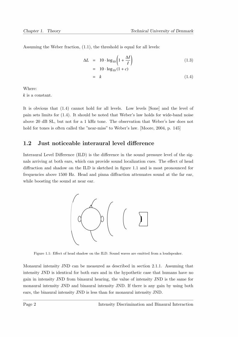
Interaural Level Difference (ILD) is the difference in the sound pressure level of the sig-nals arriving at both ears, which can provide sound localization cues. The effect of headdiffraction and shadow on the ILD is sketched in figure 1.1 and is most pronounced forfrequencies above 1500 Hz. Head and pinna diffraction attenuates sound at the far ear,while boosting the sound at near ear.

Figure 1.1: Effect of head shadow on the ILD. Sound waves are emitted from a loudspeaker.

Monaural intensity JND can be measured as described in section 2.1.1. Assuming thatintensity JND is identical for both ears and in the hypothetic case that humans have nogain in intensity JND from binaural hearing, the value of intensity JND is the same formonaural intensity JND and binaural intensity JND. If there is any gain by using bothears, the binaural intensity JND is less than for monaural intensity JND.

Page 2 Intensity Discrimination and Binaural Interaction


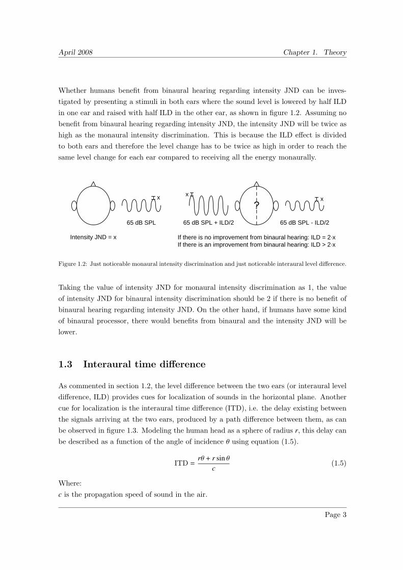
Whether humans benefit from binaural hearing regarding intensity JND can be inves-tigated by presenting a stimuli in both ears where the sound level is lowered by half ILDin one ear and raised with half ILD in the other ear, as shown in figure 1.2. Assuming nobenefit from binaural hearing regarding intensity JND, the intensity JND will be twice ashigh as the monaural intensity discrimination. This is because the ILD effect is dividedto both ears and therefore the level change has to be twice as high in order to reach thesame level change for each ear compared to receiving all the energy monaurally.

65 dB SPL 65 dB SPL + ILD/2 65 dB SPL - ILD/2

If there is no improvement from binaural hearing: ILD = 2·xIf there is an improvement from binaural hearing: ILD > 2·x

Intensity JND = x

?x x

x

Figure 1.2: Just noticeable monaural intensity discrimination and just noticeable interaural level difference.

Taking the value of intensity JND for monaural intensity discrimination as 1, the valueof intensity JND for binaural intensity discrimination should be 2 if there is no benefit ofbinaural hearing regarding intensity JND. On the other hand, if humans have some kindof binaural processor, there would benefits from binaural and the intensity JND will belower.

1.3 Interaural time difference

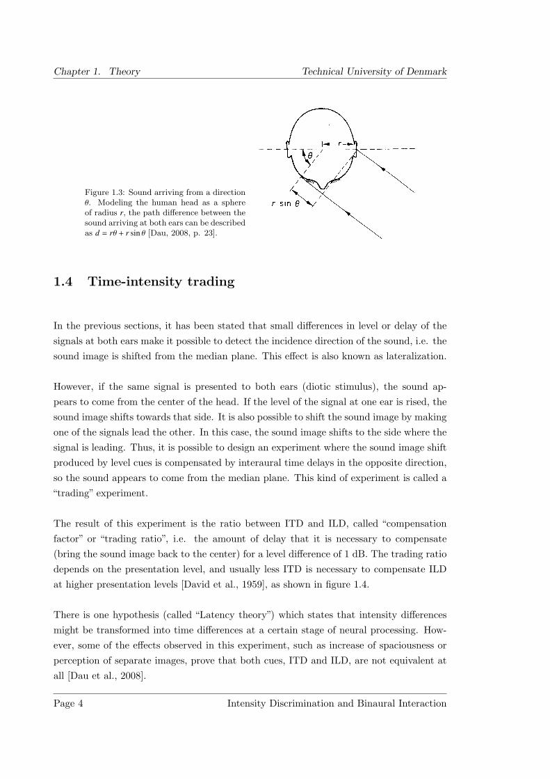
As commented in section 1.2, the level difference between the two ears (or interaural leveldifference, ILD) provides cues for localization of sounds in the horizontal plane. Anothercue for localization is the interaural time difference (ITD), i.e. the delay existing betweenthe signals arriving at the two ears, produced by a path difference between them, as canbe observed in figure 1.3. Modeling the human head as a sphere of radius r, this delay canbe described as a function of the angle of incidence θ using equation (1.5).

ITD =rθ + r sin θ

c(1.5)

Where:c is the propagation speed of sound in the air.

Page 3


Figure 1.3: Sound arriving from a directionθ. Modeling the human head as a sphereof radius r, the path difference between thesound arriving at both ears can be describedas d = rθ + r sin θ [Dau, 2008, p. 23].

1.4 Time-intensity trading

In the previous sections, it has been stated that small differences in level or delay of thesignals at both ears make it possible to detect the incidence direction of the sound, i.e. thesound image is shifted from the median plane. This effect is also known as lateralization.

However, if the same signal is presented to both ears (diotic stimulus), the sound ap-pears to come from the center of the head. If the level of the signal at one ear is rised, thesound image shifts towards that side. It is also possible to shift the sound image by makingone of the signals lead the other. In this case, the sound image shifts to the side where thesignal is leading. Thus, it is possible to design an experiment where the sound image shiftproduced by level cues is compensated by interaural time delays in the opposite direction,so the sound appears to come from the median plane. This kind of experiment is called a“trading” experiment.

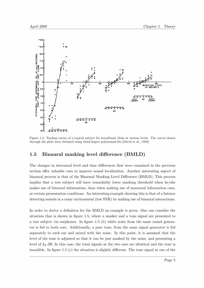
The result of this experiment is the ratio between ITD and ILD, called “compensationfactor” or “trading ratio”, i.e. the amount of delay that it is necessary to compensate(bring the sound image back to the center) for a level difference of 1 dB. The trading ratiodepends on the presentation level, and usually less ITD is necessary to compensate ILDat higher presentation levels [David et al., 1959], as shown in figure 1.4.

There is one hypothesis (called “Latency theory”) which states that intensity differencesmight be transformed into time differences at a certain stage of neural processing. How-ever, some of the effects observed in this experiment, such as increase of spaciousness orperception of separate images, prove that both cues, ITD and ILD, are not equivalent atall [Dau et al., 2008].



Figure 1.4: Trading curves of a typical subject for broadband clicks at various levels. The curves drawnthrough the plots were obtained using third-degree polynomial fits [David et al., 1959].

1.5 Binaural masking level difference (BMLD)

The changes in interaural level and time differences that were examined in the previoussection offer valuable cues to improve sound localization. Another interesting aspect ofbinaural process is that of the Binaural Masking Level Difference (BMLD). This processimplies that a test subject will have remarkably lower masking threshold when he/shemakes use of binaural information, than when making use of monaural information cues,at certain presentation conditions. An interesting example showing this is that of a listenerdetecting sounds in a noisy environment (low SNR) by making use of binaural interactions.

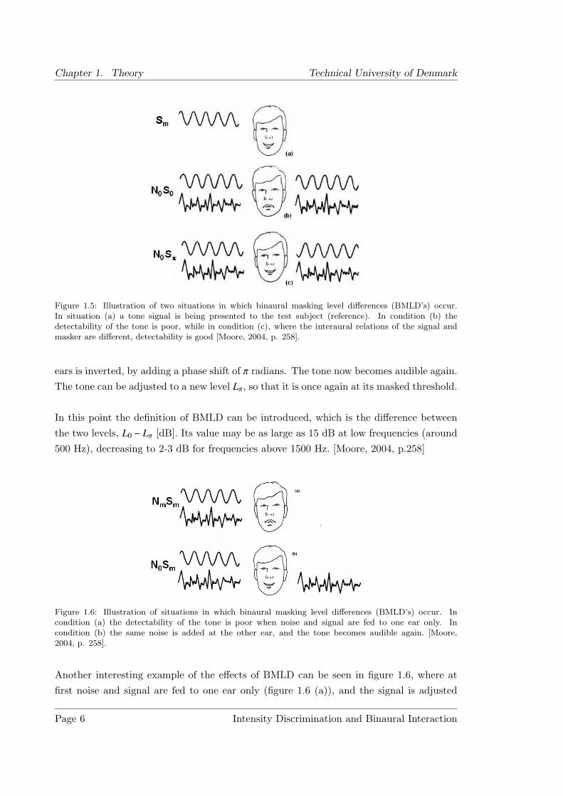
In order to derive a definition for the BMLD an example is given. One can consider thesituation that is shown in figure 1.5, where a masker and a tone signal are presented toa test subject via earphones. In figure 1.5 (b) white noise from the same sound genera-tor is fed to both ears. Additionally, a pure tone, from the same signal generator is fedseparately to each ear and mixed with the noise. In this point, it is assumed that thelevel of the tone is adjusted so that it can be just masked by the noise, and presenting alevel of L0 dB. In this case, the total signals at the two ears are identical and the tone isinaudible. In figure 1.5 (c) the situation is slightly different. The tone signal at one of the

Page 5


Figure 1.5: Illustration of two situations in which binaural masking level differences (BMLD’s) occur.In situation (a) a tone signal is being presented to the test subject (reference). In condition (b) thedetectability of the tone is poor, while in condition (c), where the interaural relations of the signal andmasker are different, detectability is good [Moore, 2004, p. 258].

ears is inverted, by adding a phase shift of π radians. The tone now becomes audible again.The tone can be adjusted to a new level Lπ, so that it is once again at its masked threshold.

In this point the definition of BMLD can be introduced, which is the difference betweenthe two levels, L0 − Lπ [dB]. Its value may be as large as 15 dB at low frequencies (around500 Hz), decreasing to 2-3 dB for frequencies above 1500 Hz. [Moore, 2004, p.258]

Figure 1.6: Illustration of situations in which binaural masking level differences (BMLD’s) occur. Incondition (a) the detectability of the tone is poor when noise and signal are fed to one ear only. Incondition (b) the same noise is added at the other ear, and the tone becomes audible again. [Moore,2004, p. 258].

Another interesting example of the effects of BMLD can be seen in figure 1.6, where atfirst noise and signal are fed to one ear only (figure 1.6 (a)), and the signal is adjusted



to be at its masked threshold, thus inaudible. Then, if the same noise is added at theother ear (figure 1.6 (b)), the tone becomes audible again. This implies that by addingnoise at the ear where no signal is present the tone becomes more detectable. This noise,however should be correlated with the masker at the other ear. Uncorrelated maskers willnot result in BMLD.

It is important to note that BMLD phenomenon is not limited to pure tone signals but itis also observed for complex signals too (complex tones, clicks and speech sounds).

Over the years, many different models have been proposed to account for the variousaspects of binaural processing [Moore, 2004, p.263]. Durlach presented a rather simplemodel that was able to describe the BMLD phenomenon. This model was based on theEqualization - Cancellation (EC) concept. That is based on the idea that the auditorysystem tries to eliminate the masker by manipulating the stimuli between the two ears,until the masker components are equal (equalization) and then subtracts them so thatthey cancel each other (cancellation) [Dau et al., 2008].

The first step of this model (equalization process) involves amplification or attenuationof the stimuli and shifting in time. This is because the model needs to compensate forthe interaural level differences (ILD) and interaural time differences (ITD). In order totake into consideration the finite limit of the BMLD phenomenon the model assumes animperfect equalization process. This assumption is realized by introducing two sources oferror: jitter in the amplification (ε) and shifting in time (δ). ε and δ are asummed tobe statistically independent random variables, with zero mean and variances σ2

ε and σ2δ

respectively. Under those assumptions, Durlach [Dau et al., 2008] was able to show thatthe difference between the N0S 0 and N0S π condition can be described by the followingequation:

BMLD(N0S 0 − N0S π) = 10 log10

1 +2e−ω

20σ

2δ

1 + σ2ε − e−ω

20σ

2δ

(1.6)

where:

ω0 is the center frequency (in radians) of the auditory filter with the stimulus. Fromequation (1.6) it is possible to note that for very low frequencies:

limω0→0BMLD(N0S 0 − N0S π) = 10 log10

(1 +

2σ2ε

)(1.7)

Page 7


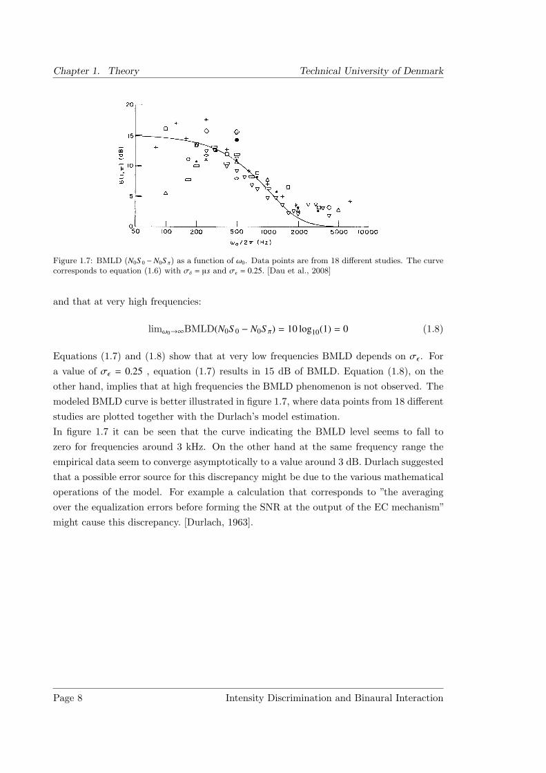
Figure 1.7: BMLD (N0S 0 − N0S π) as a function of ω0. Data points are from 18 different studies. The curvecorresponds to equation (1.6) with σδ = µs and σε = 0.25. [Dau et al., 2008]

and that at very high frequencies:

limω0→∞BMLD(N0S 0 − N0S π) = 10 log10(1) = 0 (1.8)

Equations (1.7) and (1.8) show that at very low frequencies BMLD depends on σε . Fora value of σε = 0.25 , equation (1.7) results in 15 dB of BMLD. Equation (1.8), on theother hand, implies that at high frequencies the BMLD phenomenon is not observed. Themodeled BMLD curve is better illustrated in figure 1.7, where data points from 18 differentstudies are plotted together with the Durlach’s model estimation.In figure 1.7 it can be seen that the curve indicating the BMLD level seems to fall tozero for frequencies around 3 kHz. On the other hand at the same frequency range theempirical data seem to converge asymptotically to a value around 3 dB. Durlach suggestedthat a possible error source for this discrepancy might be due to the various mathematicaloperations of the model. For example a calculation that corresponds to ”the averagingover the equalization errors before forming the SNR at the output of the EC mechanism”might cause this discrepancy. [Durlach, 1963].


April 2008 Chapter 2. Results

Chapter 2Results

2.1 Intensity discrimination

2.1.1 Monaural intensity discrimination

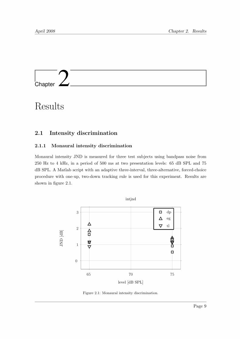
Monaural intensity JND is measured for three test subjects using bandpass noise from250 Hz to 4 kHz, in a period of 500 ms at two presentation levels: 65 dB SPL and 75dB SPL. A Matlab script with an adaptive three-interval, three-alternative, forced-choiceprocedure with one-up, two-down tracking rule is used for this experiment. Results areshown in figure 2.1.

intjnd

level [dB SPL]

JND

[dB

]

dp

eg

tl

65 70 75

0

1

2

3

Figure 2.1: Monaural intensity discrimination.

Page 9

Chapter 2. Results Technical University of Denmark

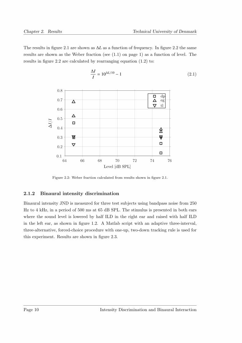
The results in figure 2.1 are shown as ∆L as a function of frequency. In figure 2.2 the sameresults are shown as the Weber fraction (see (1.1) on page 1) as a function of level. Theresults in figure 2.2 are calculated by rearranging equation (1.2) to:

∆II

= 10∆L/10 − 1 (2.1)

Level [dB SPL]

∆I/I

dpegtl

64 66 68 70 72 74 760.1

0.2

0.3

0.4

0.5

0.6

0.7

0.8

Figure 2.2: Weber fraction calculated from results shown in figure 2.1.

2.1.2 Binaural intensity discrimination

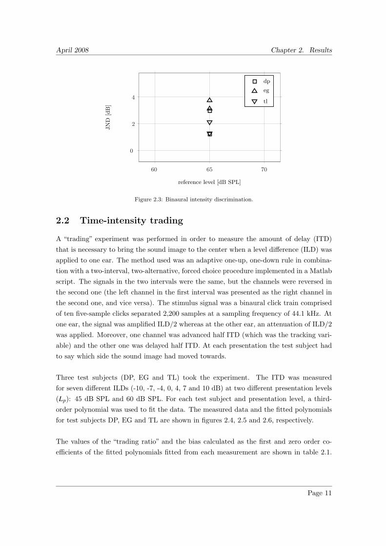
Binaural intensity JND is measured for three test subjects using bandpass noise from 250Hz to 4 kHz, in a period of 500 ms at 65 dB SPL. The stimulus is presented in both earswhere the sound level is lowered by half ILD in the right ear and raised with half ILDin the left ear, as shown in figure 1.2. A Matlab script with an adaptive three-interval,three-alternative, forced-choice procedure with one-up, two-down tracking rule is used forthis experiment. Results are shown in figure 2.3.



reference level [dB SPL]

JN

D[d

B]

dp

eg

tl

60 65 70

0

2

4

Figure 2.3: Binaural intensity discrimination.


A “trading” experiment was performed in order to measure the amount of delay (ITD)that is necessary to bring the sound image to the center when a level difference (ILD) wasapplied to one ear. The method used was an adaptive one-up, one-down rule in combina-tion with a two-interval, two-alternative, forced choice procedure implemented in a Matlabscript. The signals in the two intervals were the same, but the channels were reversed inthe second one (the left channel in the first interval was presented as the right channel inthe second one, and vice versa). The stimulus signal was a binaural click train comprisedof ten five-sample clicks separated 2,200 samples at a sampling frequency of 44.1 kHz. Atone ear, the signal was amplified ILD/2 whereas at the other ear, an attenuation of ILD/2was applied. Moreover, one channel was advanced half ITD (which was the tracking vari-able) and the other one was delayed half ITD. At each presentation the test subject hadto say which side the sound image had moved towards.

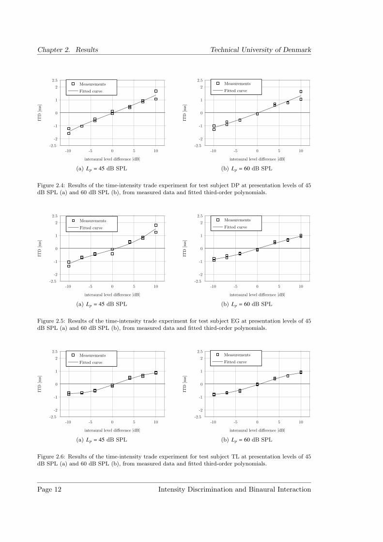
Three test subjects (DP, EG and TL) took the experiment. The ITD was measuredfor seven different ILDs (-10, -7, -4, 0, 4, 7 and 10 dB) at two different presentation levels(Lp): 45 dB SPL and 60 dB SPL. For each test subject and presentation level, a third-order polynomial was used to fit the data. The measured data and the fitted polynomialsfor test subjects DP, EG and TL are shown in figures 2.4, 2.5 and 2.6, respectively.

The values of the “trading ratio” and the bias calculated as the first and zero order co-efficients of the fitted polynomials fitted from each measurement are shown in table 2.1.

Page 11


interaural level difference [dB]

ITD

[ms]

Measurements

Fitted curve

-10 -5 0 5 10-2.5

-2

-1

0

1

2

2.5

(a) Lp = 45 dB SPL


ITD

[ms]

Measurements

Fitted curve

-10 -5 0 5 10-2.5

-2

-1

0

1

2

2.5

(b) Lp = 60 dB SPL

Figure 2.4: Results of the time-intensity trade experiment for test subject DP at presentation levels of 45dB SPL (a) and 60 dB SPL (b), from measured data and fitted third-order polynomials.


ITD

[ms]

Measurements

Fitted curve

-10 -5 0 5 10-2.5

-2

-1

0

1

2

2.5

(a) Lp = 45 dB SPL


ITD

[ms]

Measurements

Fitted curve

-10 -5 0 5 10-2.5

-2

-1

0

1

2

2.5

(b) Lp = 60 dB SPL

Figure 2.5: Results of the time-intensity trade experiment for test subject EG at presentation levels of 45dB SPL (a) and 60 dB SPL (b), from measured data and fitted third-order polynomials.


ITD

[ms]

Measurements

Fitted curve

-10 -5 0 5 10-2.5

-2

-1

0

1

2

2.5

(a) Lp = 45 dB SPL


ITD

[ms]

Measurements

Fitted curve

-10 -5 0 5 10-2.5

-2

-1

0

1

2

2.5

(b) Lp = 60 dB SPL

Figure 2.6: Results of the time-intensity trade experiment for test subject TL at presentation levels of 45dB SPL (a) and 60 dB SPL (b), from measured data and fitted third-order polynomials.



45 dB SPL 60 dB SPLTest subject Trading ratio [µs/dB] Bias [µs] Trading ratio [µs/dB] Bias [µs]

DP 5.68 -1.49 5.60 -1.73EG 4.33 -4.10 4.57 -1.27TL 5.22 -3.30 5.04 -2.68

Table 2.1: Values of the “trading ratio” and the bias, given by the first and zero order terms of thepolynomials calculated fitting the data from the time-intensity trade experiment.

2.3 Binaural Masking Level Difference

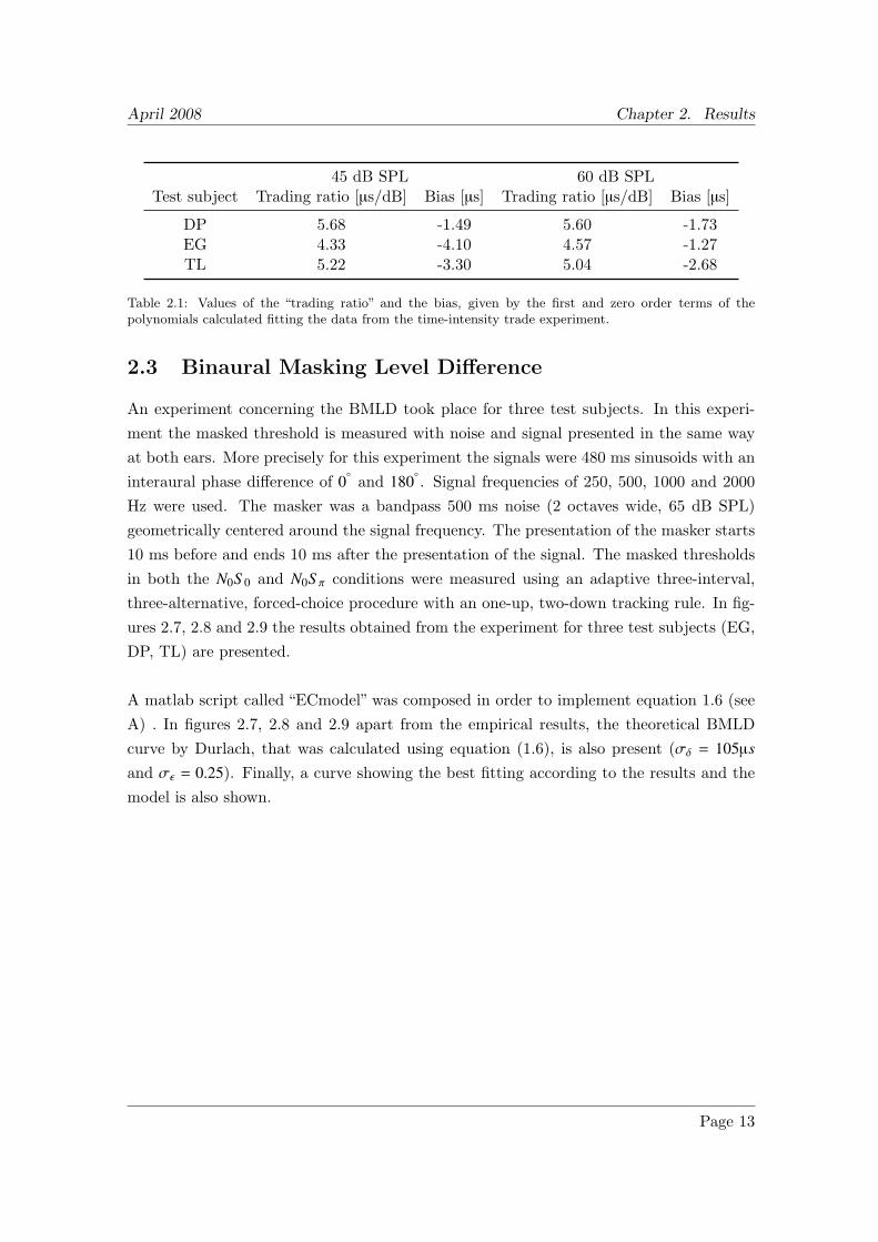
An experiment concerning the BMLD took place for three test subjects. In this experi-ment the masked threshold is measured with noise and signal presented in the same wayat both ears. More precisely for this experiment the signals were 480 ms sinusoids with aninteraural phase difference of 0

◦

and 180◦

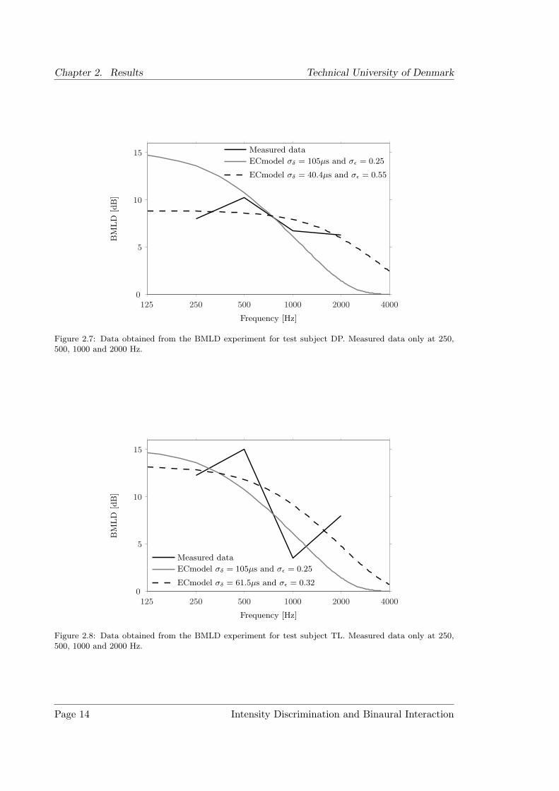
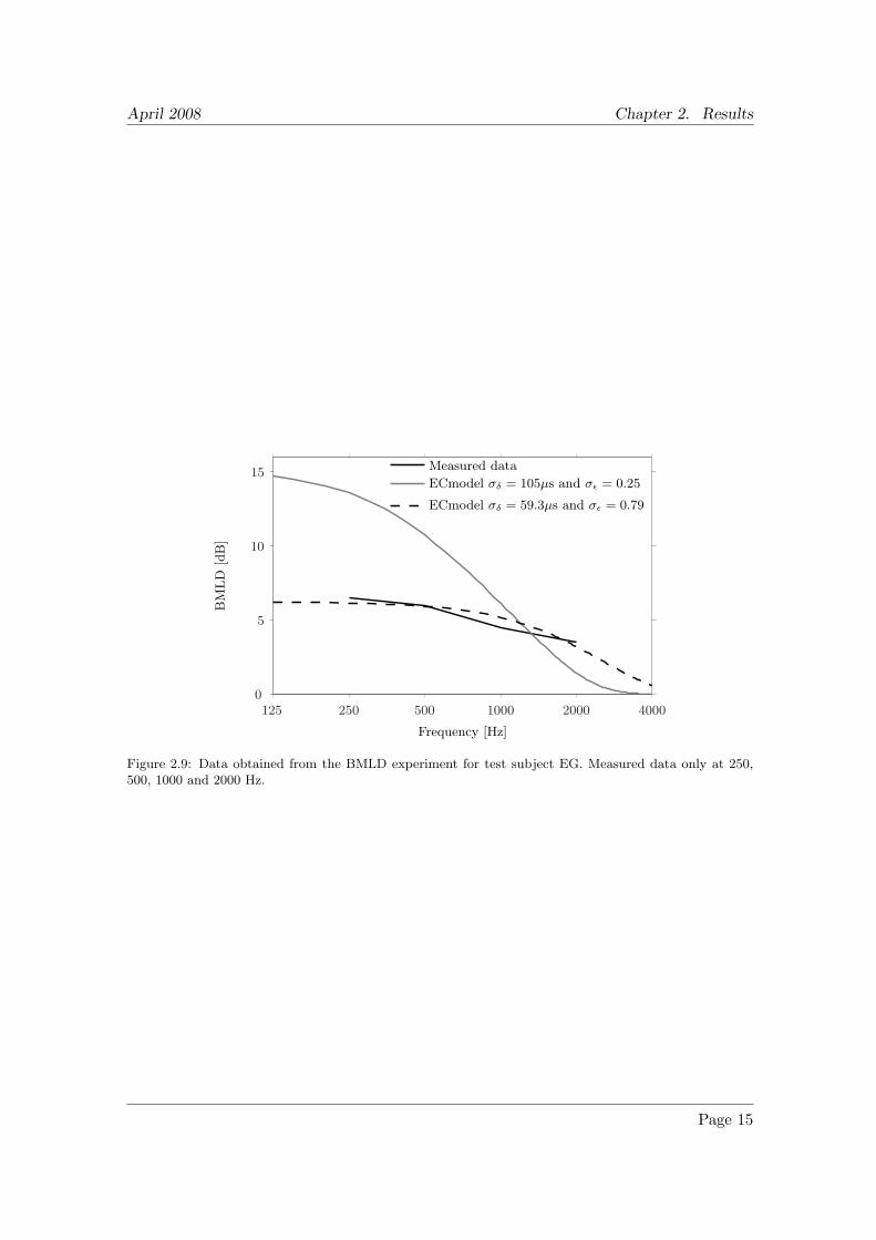
. Signal frequencies of 250, 500, 1000 and 2000Hz were used. The masker was a bandpass 500 ms noise (2 octaves wide, 65 dB SPL)geometrically centered around the signal frequency. The presentation of the masker starts10 ms before and ends 10 ms after the presentation of the signal. The masked thresholdsin both the N0S 0 and N0S π conditions were measured using an adaptive three-interval,three-alternative, forced-choice procedure with an one-up, two-down tracking rule. In fig-ures 2.7, 2.8 and 2.9 the results obtained from the experiment for three test subjects (EG,DP, TL) are presented.

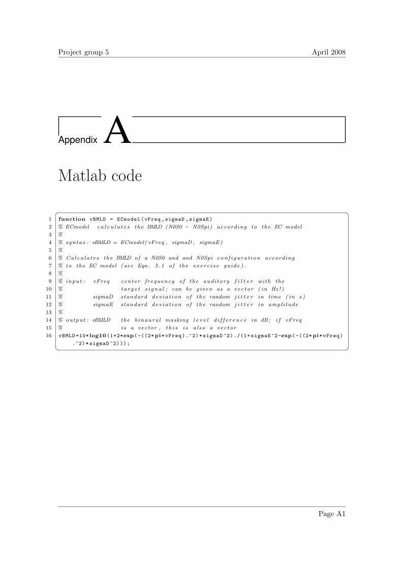
A matlab script called “ECmodel” was composed in order to implement equation 1.6 (seeA) . In figures 2.7, 2.8 and 2.9 apart from the empirical results, the theoretical BMLDcurve by Durlach, that was calculated using equation (1.6), is also present (σδ = 105µs

and σε = 0.25). Finally, a curve showing the best fitting according to the results and themodel is also shown.

Page 13


Frequency [Hz]

BM

LD

[dB

]

Measured data

ECmodel σδ = 105µs and σε = 0.25

ECmodel σδ = 40.4µs and σε = 0.55

125 250 500 1000 2000 40000

5

10

15

Figure 2.7: Data obtained from the BMLD experiment for test subject DP. Measured data only at 250,500, 1000 and 2000 Hz.

Frequency [Hz]

BM

LD

[dB

]

Measured data



125 250 500 1000 2000 40000

5

10

15

Figure 2.8: Data obtained from the BMLD experiment for test subject TL. Measured data only at 250,500, 1000 and 2000 Hz.



Frequency [Hz]

BM

LD

[dB

]

Measured data



125 250 500 1000 2000 40000

5

10

15

Figure 2.9: Data obtained from the BMLD experiment for test subject EG. Measured data only at 250,500, 1000 and 2000 Hz.

Page 15

April 2008 Chapter 3. Discussion

Chapter 3Discussion

3.1 Interaural level discrimination

Weber´s law states that the intensity JND should be the same for any levels as seen inequation (1.4). In figure 2.1 the results for monaural intensity JND as a function of twolevels can be seen. It can be noted that equation (1.4) only holds for test subject TL.For the other two test subjects the JND became lower for 75 dB SPL. This can perhapsbe explained by the presence of fluctuating background noise and the reduced set of data(average values calculated from 2 measurements).

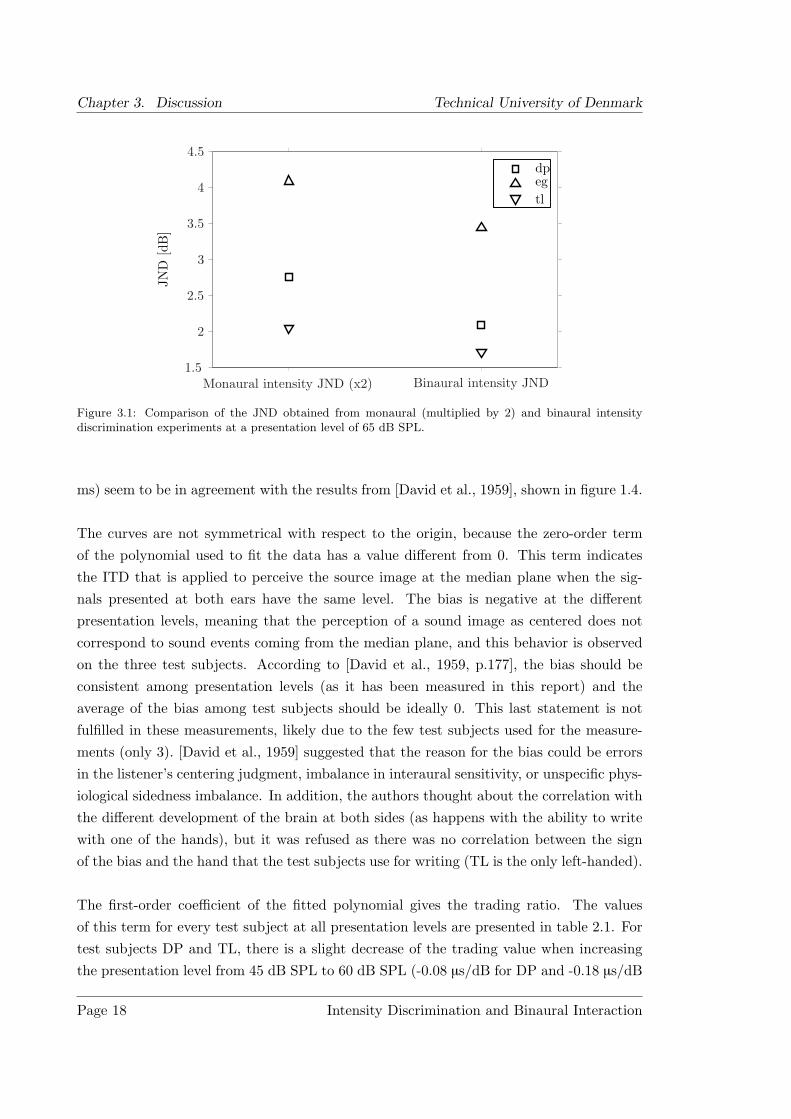
In figure 3.1 the results from monaural and binaural intensity discrimination are com-pared. It can be seen that the binaural intensity JND is less than twice as high as themonaural intensity JND for each test subject. This proves that all three test subjectsbenefit from binaural hearing and have some kind of binaural processor. During the bin-aural intensity discrimination experiment the test subjects described the noise as one fusedobject. They also mentioned that the method by itself was not good. It is surprisinglydifficult to press the right button (to indicate that the change was in the last interval)when the sound was moving to the left. A perhaps better way to perform the experimentis to have an instructor that will note in which interval the noise moves to the left, so thetest subject only has to say interval one, two or three to indicate the interval and therebypreventing any confusions between left and right.


The results of the trading experiment are presented in figures 2.4, 2.5 and 2.6 in sec-tion 2.2. The variability of the data and the range of ITD values (between -2 ms and 2

Page 17

Chapter 3. Discussion Technical University of Denmark

JND

[dB

]dpegtl

Monaural intensity JND (x2) Binaural intensity JND1.5

2

2.5

3

3.5

4

4.5

Figure 3.1: Comparison of the JND obtained from monaural (multiplied by 2) and binaural intensitydiscrimination experiments at a presentation level of 65 dB SPL.

ms) seem to be in agreement with the results from [David et al., 1959], shown in figure 1.4.

The curves are not symmetrical with respect to the origin, because the zero-order termof the polynomial used to fit the data has a value different from 0. This term indicatesthe ITD that is applied to perceive the source image at the median plane when the sig-nals presented at both ears have the same level. The bias is negative at the differentpresentation levels, meaning that the perception of a sound image as centered does notcorrespond to sound events coming from the median plane, and this behavior is observedon the three test subjects. According to [David et al., 1959, p.177], the bias should beconsistent among presentation levels (as it has been measured in this report) and theaverage of the bias among test subjects should be ideally 0. This last statement is notfulfilled in these measurements, likely due to the few test subjects used for the measure-ments (only 3). [David et al., 1959] suggested that the reason for the bias could be errorsin the listener’s centering judgment, imbalance in interaural sensitivity, or unspecific phys-iological sidedness imbalance. In addition, the authors thought about the correlation withthe different development of the brain at both sides (as happens with the ability to writewith one of the hands), but it was refused as there was no correlation between the signof the bias and the hand that the test subjects use for writing (TL is the only left-handed).

The first-order coefficient of the fitted polynomial gives the trading ratio. The valuesof this term for every test subject at all presentation levels are presented in table 2.1. Fortest subjects DP and TL, there is a slight decrease of the trading value when increasingthe presentation level from 45 dB SPL to 60 dB SPL (-0.08 µs/dB for DP and -0.18 µs/dB


April 2008 Chapter 3. Discussion

for TL). In contrast, the trading value increases for EG (0.25 µs/dB) under the same con-ditions, differing from the predictions by [David et al., 1959], who found that the tradingratio decreased with increasing level. However, the obtained results should not lead to theconclusion that ITD and ILD are coded and interpreted by the brain in the same way,because the stimuli were not perceived as a single sound event coming from the centerof the head. The test subjects described the effects as perception of two different soundevents at both ears or “sound image broadening” instead of sound image displacementbetween the two presentations, i.e. having a clear lateralization.

3.3 Binaural masking level difference

In figures 2.7, 2.8 and 2.9 the BMLD results for the three test subjects are plotted as afunction of the stimulus frequency. In addition, the theoretical BMLD predicted by [Davidet al., 1959] with values σδ = 105µs and σε = 0.25 is plotted. The curves with the param-eters σδ and σε that offered the best fitting for the actual measurements are also plottedin each figure.

In figure 1.7 on page 8 the data obtained for 18 different test subjects deviate a lotfrom each other, resulting in a cloud of data points. Therefore, the expected variabil-ity among test subjects is high, and the equation (1.6) (also plotted in the same figure)just provides an approximation to the population average. The measurements for thisreport were obtained with just one run for each frequency of the three test subjects in anoisy environment. With these sets of data, it is not possible to get statistical values thatgive precise information about the average BMLD at a certain frequency and its deviation.

However, test subject EG seems to have less benefit from BMLD as compared to thetest subjects DP and TL. In figure 2.8 the test subject TL seems to have a dip at 1 kHz.Prior to this report test subject TL has measured his audiogram which presents a dip inhearing threshold at 1 kHz which is different for each ear. This could explain the lack ofbenefit from binaural hearing at this frequency and thereby the dip in BMLD. Neverthe-less, more measurements are necessary in order to reduce the uncertainty and prove thelatest hypothesis.

Page 19

Chapter 3. Discussion Technical University of Denmark


April 2008 Chapter 4. Conclusion

Chapter 4Conclusion

In this report, the intensity discrimination and binaural interaction of the human audi-tory system have been discussed theoretically and from measurements. Intensity JND wasmeasured both monaurally and binaurally. Time-intensity trading was investigated andadditionally the effects of BMLD were examined.

The reduction in the measured binaural JND with respect to the equivalent monauralJND show that humans have a kind of binaural processor, which takes advantage frombinaural hearing detection cues.

It is possible to change the perception of the position of the source image by modify-ing the values of ITD and ILD. ITD is not processed in the same way as ILD, as thestimuli in the experiment are not perceived as single sound events at a certain location,but as separated events.

Results show that there is an improvement in the ability of detecting a signal in back-ground noise when the noise signals presented at both ears are correlated and the signalto detect is presented to just one ear or to both in antiphase. This improvement, knownas BMLD, presents values up to 15 dB in these measurements.

Page 21

Chapter 4. Conclusion Technical University of Denmark


April 2008 Bibliography

Bibliography

[Dau, 2008] Dau, T. (2008). Intensity coding and binaural processing in the auditory sys-tem. Slide show.

[Dau et al., 2008] Dau, T., Christiansen, T. U., and Santurette, S. (2008). Intensity Dis-crimination and Binaural Interaction. 1.1.2 edition.

[David et al., 1959] David, E.E., J., Guttman, N., and van Bergeijk, W. (1959). Binau-ral interaction of high-frequency complex stimuli. Journal of the Acoustical Society ofAmerica, 31(6):774–782.

[Durlach, 1963] Durlach, N. (1963). Equalization and cancellation theory of binauralmasking-level differences. Acoustical Society of America – Journal, 35(8):1206–1218.

[Moore, 2004] Moore, B. C. J. (2004). An introduction to the psychology of hearing.

Page 23

Bibliography Technical University of Denmark


Project group 5 April 2008

Appendix AMatlab code

� �1 function vBMLD = ECmodel(vFreq ,sigmaD ,sigmaE)

2 % ECmodel c a l c u l a t e s the BMLD (N0S0 − N0Spi ) according to the EC model

3 %

4 % syntax : vBMLD = ECmodel( vFreq , sigmaD , sigmaE)

5 %

6 % Ca lcu l a t e s the BMLD of a N0S0 and and N0Spi con f i gu ra t i on according

7 % to the EC model ( see Eqn . 5.1 o f the e x e r c i s e guide ) .

8 %

9 % input : vFreq center f requency o f the aud i tory f i l t e r with the

10 % ta r g e t s i g n a l ; can be g iven as a vec tor ( in Hz ! )

11 % sigmaD standard dev i a t i on o f the random j i t t e r in time ( in s )

12 % sigmaE standard dev i a t i on o f the random j i t t e r in ampl i tude

13 %

14 % output : vBMLD the b inaura l masking l e v e l d i f f e r e n c e in dB; i f vFreq

15 % i s a vector , t h i s i s a l s o a vec tor

16 vBMLD =10* log10(1+2*exp(-((2*pi*vFreq).^2)*sigmaD ^2) ./(1+ sigmaE^2-exp(-((2*pi*vFreq)

.^2)*sigmaD ^2)));� �

Page A1

Intensity Discrimination and Binaural...

Documents

Transcript of Intensity Discrimination and Binaural...