
Estimating the dose-response function through the GLM approach · 2019-09-26 · through the GLM...
32
Munich Personal RePEc Archive Estimating the dose-response function through the GLM approach Guardabascio, Barbara and Ventura, Marco Italian National Institute of Statistics (ISTAT), Italian National Institute of Statistics (ISTAT) 13 March 2013 Online at https://mpra.ub.uni-muenchen.de/45013/ MPRA Paper No. 45013, posted 13 Mar 2013 17:44 UTC
Transcript of Estimating the dose-response function through the GLM approach · 2019-09-26 · through the GLM...
Munich Personal RePEc Archive
Estimating the dose-response function
through the GLM approach
Guardabascio, Barbara and Ventura, Marco
Italian National Institute of Statistics (ISTAT), Italian NationalInstitute of Statistics (ISTAT)
13 March 2013
Online at https://mpra.ub.uni-muenchen.de/45013/
MPRA Paper No. 45013, posted 13 Mar 2013 17:44 UTC
Estimating the dose-response function
through the GLM approach
Barbara GuardabascioISTAT, Italian National Institute of Statistics
Rome, [email protected]
Marco VenturaISTAT, Italian National Institute of Statistics
Rome, [email protected]
Abstract. This paper revises the estimation of the dose-response functionas in Hirano and Imbens (2004) by proposing a flexible way to estimate thegeneralized propensity score when the treatment variable is not necessarilynormally distributed. We also provide a set of programs that accomplishthis task by using the GLM in the first step of the computation.
Keywords: generalized propensity score, GLM, dose-response, continuoustreatment, bias removal
1 IntroductionHow effective are policy programs with continuous treatment exposure? An-swering this question essentially amounts to estimate a dose-response functionas proposed in Hirano and Imbens (2004). Whenever doses are not randomlyassigned, but are given under experimental conditions, estimation of a dose-response function is possible using the Generalized Propensity Score (GPS).The GPS for continuous treatment is an extension of the popular propensityscore methodology for binary treatments (Rosenbaum and Rubin, 1983, 1984)and multi-valued treatments (Imbens, 2000; Lechner, 2001). Indeed, Hiranoand Imbens show that the GPS has a balancing property similar to the bi-nary propensity score. Conditional on observable characteristics, the level ofthe treatment can be considered as random for units belonging to the sameGPS strata. It means that adjusting for the GPS removes all biases associ-ated with differences in the covariates. Since its formulation, the GPS has beenrepeatedly used in observational studies and ad hoc programs have been pro-vided for STATA users doseresponse.ado and gpscore.ado by Bia and Mat-tei (2008), henceforth BM. However, many applied works (Fryges and Wagner,2008; Fryges, 2009) remark that the treatment variable may be not normallydistributed. In this case the BM programs are not usable as they do not allowfor different distribution assumptions other than the normal density.In this paper we overcome this problem. Building on BM programs we provide anew set of STATA programs, doseresponse2.ado and gpscore2.ado, which al-lows to accommodate different distribution functions of the treatment variable.This task is accomplished through by the application of the Generalized Lineal
1
Models estimator, GLM, in the first step instead of the Maximum Likelihood,ML, for normal distribution.
In order to easily compare our programs with the BM ones, we use the samedataset used by BM and originally collected by Imbens et al (2001). The sampleis made up of individuals winning the Megabucks lottery in Massachusetts in themid-1980’s. The main source of potential bias is the unit and item nonresponse.Hirano and Imbens (2004) claim that it is possible to prove that the nonresponsewas non-random. The missing data imply that the amount of the prize is po-tentially correlated with background characteristics and potential outcomes. Itmay be useful to remind that using these bias reducing techniques, it is possibleto reduce, not to eliminate the bias generated by unobservable heterogeneity.The extent to which unconfoundedness holds, namely the extent to which thebias is reduced, depends on the quality of the database used to compute theGPS. This caveat is independent of the particular distribution function one iswilling to assume for the treatment variable.
The reminder of the paper proceeds as follows. Section 2 briefly reviews theestimation of the dose-response function. Section 3 introduces the GLM andexplains how to use it to fit the GPS. Section 3.1. analyzes flogit, a special case ofparticular interest in economics. Section 4 describes how the programs work stepby step. Section 5 and 6 list the syntax and the options, respectively. Section 7presents an application of the programs using some non-normal distribution ofthe treatment variable. Section 8 concludes.
2 A brief review of the econometrics of the dose-
response functionLet us define a set of potential outcomes {Yi(t)} for t ∈ T , where T representsthe continuous set of potential treatments defined over the interval [t0, t1], andYi(t) is referred to as the unit-level dose-response function.
Let us suppose to have a random sample of N units. For each unit i weobserve a k × 1 vector of pre-treatment covariates, Xi, the level of the treat-ment delivered, Ti, and the outcome corresponding to the level of the treatmentreceived, Yi = Yi(Ti). We are interested in the average dose-response functionψ(t) = E[Yi(t)].
Under some regularity conditions1 of {Yi(t)}, Xi, and Ti Hirano and Imbensdefine the propensity function as the conditional density of the actual treatmentgiven the covariates. More in detail, if we define as r(t, x) = fT |X(t|x) theconditional density function of the treatment given the covariates, then theGPS is
R = r(T |X)
The balancing property can be defined similarly to the binary case. Thatis, within strata with the same value of r(t, x), the probability that T = t does
1For each i, {Yi(t)}, Xi and Ti are supposed to be defined on a common probability space,Ti is continuously distributed with respect to Lebsgue measure on T , and Yi = Yi(Ti) is awell defined random variable.
2
not depend on the value of X:
X⊥1{T = t}|r(t, x)
This balancing property, along with unconfoundedness implies that assignmentto treatment is unconfounded given the GPS. If weak unconfoundedness as-sumption holds, given the pre-treatment variables X, we have:
Y (t)⊥T |X ∀t ∈ T
then, for every tfT (t|r(t,X), Y (t)) = fT (t|r(t,X))
this means that the GPS can be used to eliminate any bias associated withdifferences in the covariates (for a formal proof see Theorem 2.1 and 3.1 of Hiranoand Imbens, 2004). Therefore, the dose-response function can be obtained as
γ(t, r) = E[Y (t)|r(t,X) = r] = E[Y |T = t, R = r] (1)
ψ(t) = E[γ(t, r(t,X))] (2)
Practical implementation of the GPS is accomplished in three steps2.In the first step the score r(t, x) is estimated. In the second step the con-
ditional expectation of the outcome as a function of two scalar variables, thetreatment level T and the GPS R, is estimated, E[Y |T = t, R = r]. In the thirdstep the dose-response function, ψ(t) = E[(t, r(t,X))], t ∈ T , is estimated byaveraging the estimated conditional expectation, γ(t, r(t,X)), over the GPS ateach level of the treatment one is interested in.
As the second and the third step in our programs replicate BM’s program,we refer to it for more details about these steps. While, we will devote moreattention in explaining how our programs implement the first step to computethe score r(t, x).
3 Estimation of the score through the GLMIn many economic applications T cannot be supposed to be normally dis-tributed and assuming a normal distribution of the treatment given the co-variates, Ti|Xi ∼ N(β′Xi, σ
2) where β is k×1 vector of parameters, has severaldrawbacks. The problem is not new in the econometric literature, think aboutcount, binomial, fractional and survival data, just to cite a few (see Wooldridge2002 for a comprehensive review of this topic). Taking into account what be-fore, we aim to go beyond these problems presenting a possible solution to theestimation of the GPS in these cases. Our idea consists in replacing the linearregression3 by the GLM developed by McCullagh and Nelder (1989) in the firststep to estimate the dose-response, and to retrieve the GPS from the exponential
2Hirano and Imbens and BM use the notation µ instead of ψ and β instead of γ. We haveslightly changed notation in order to avoid confusion in the following Sections.
3Precisely, the programs by BM estimate the GPS assuming T |X or some transformationsof T , g(T )|X, normally distributed. The estimation of β is performed through the ML.
3
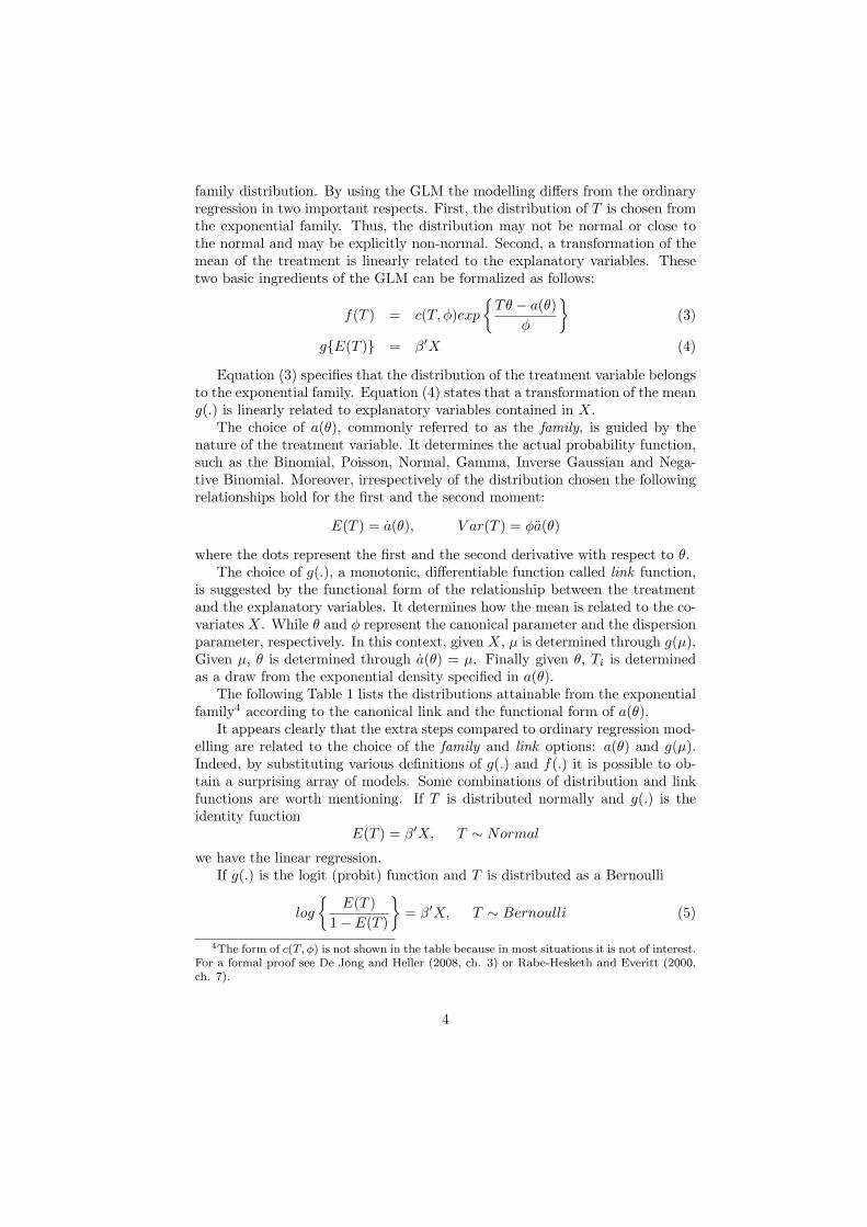
family distribution. By using the GLM the modelling differs from the ordinaryregression in two important respects. First, the distribution of T is chosen fromthe exponential family. Thus, the distribution may not be normal or close tothe normal and may be explicitly non-normal. Second, a transformation of themean of the treatment is linearly related to the explanatory variables. Thesetwo basic ingredients of the GLM can be formalized as follows:
f(T ) = c(T, φ)exp
{Tθ − a(θ)
φ
}(3)
g{E(T )} = β′X (4)
Equation (3) specifies that the distribution of the treatment variable belongsto the exponential family. Equation (4) states that a transformation of the meang(.) is linearly related to explanatory variables contained in X.
The choice of a(θ), commonly referred to as the family, is guided by thenature of the treatment variable. It determines the actual probability function,such as the Binomial, Poisson, Normal, Gamma, Inverse Gaussian and Nega-tive Binomial. Moreover, irrespectively of the distribution chosen the followingrelationships hold for the first and the second moment:
E(T ) = a(θ), V ar(T ) = φa(θ)
where the dots represent the first and the second derivative with respect to θ.The choice of g(.), a monotonic, differentiable function called link function,
is suggested by the functional form of the relationship between the treatmentand the explanatory variables. It determines how the mean is related to the co-variates X. While θ and φ represent the canonical parameter and the dispersionparameter, respectively. In this context, given X, µ is determined through g(µ).Given µ, θ is determined through a(θ) = µ. Finally given θ, Ti is determinedas a draw from the exponential density specified in a(θ).
The following Table 1 lists the distributions attainable from the exponentialfamily4 according to the canonical link and the functional form of a(θ).
It appears clearly that the extra steps compared to ordinary regression mod-elling are related to the choice of the family and link options: a(θ) and g(µ).Indeed, by substituting various definitions of g(.) and f(.) it is possible to ob-tain a surprising array of models. Some combinations of distribution and linkfunctions are worth mentioning. If T is distributed normally and g(.) is theidentity function
E(T ) = β′X, T ∼ Normal
we have the linear regression.If g(.) is the logit (probit) function and T is distributed as a Bernoulli
log
{E(T )
1− E(T )
}= β′X, T ∼ Bernoulli (5)
4The form of c(T, φ) is not shown in the table because in most situations it is not of interest.For a formal proof see De Jong and Heller (2008, ch. 3) or Rabe-Hesketh and Everitt (2000,ch. 7).
4
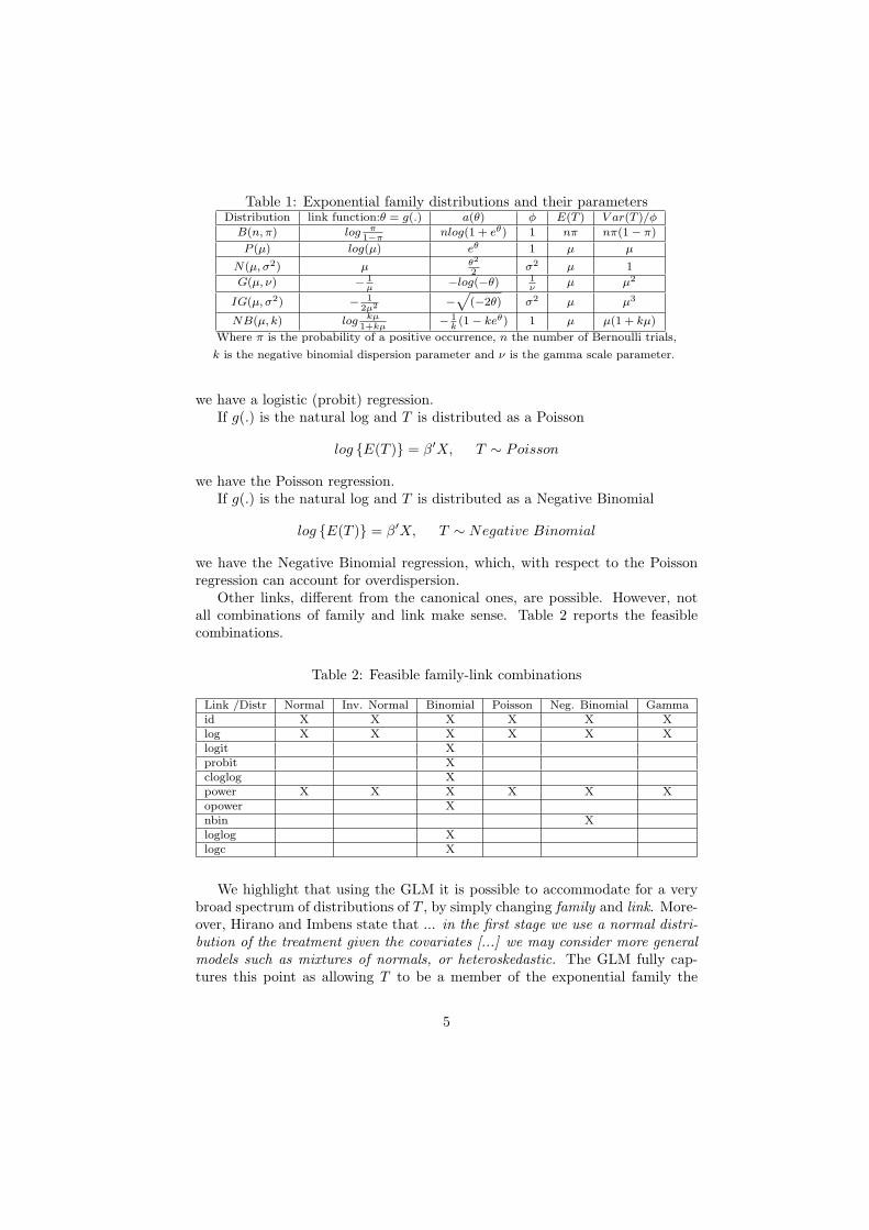
Table 1: Exponential family distributions and their parametersDistribution link function:θ = g(.) a(θ) φ E(T ) V ar(T )/φ
B(n, π) log π1−π
nlog(1 + eθ) 1 nπ nπ(1− π)
P (µ) log(µ) eθ 1 µ µ
N(µ, σ2) µ θ2
2σ2 µ 1
G(µ, ν) − 1
µ−log(−θ) 1
νµ µ2
IG(µ, σ2) − 1
2µ2−√
(−2θ) σ2 µ µ3
NB(µ, k) log kµ
1+kµ− 1
k(1− keθ) 1 µ µ(1 + kµ)
Where π is the probability of a positive occurrence, n the number of Bernoulli trials,
k is the negative binomial dispersion parameter and ν is the gamma scale parameter.
we have a logistic (probit) regression.If g(.) is the natural log and T is distributed as a Poisson
log {E(T )} = β′X, T ∼ Poisson
we have the Poisson regression.If g(.) is the natural log and T is distributed as a Negative Binomial
log {E(T )} = β′X, T ∼ Negative Binomial
we have the Negative Binomial regression, which, with respect to the Poissonregression can account for overdispersion.
Other links, different from the canonical ones, are possible. However, notall combinations of family and link make sense. Table 2 reports the feasiblecombinations.
Table 2: Feasible family-link combinations
Link /Distr Normal Inv. Normal Binomial Poisson Neg. Binomial Gammaid X X X X X Xlog X X X X X Xlogit Xprobit Xcloglog Xpower X X X X X Xopower Xnbin Xloglog Xlogc X
We highlight that using the GLM it is possible to accommodate for a verybroad spectrum of distributions of T , by simply changing family and link. More-over, Hirano and Imbens state that ... in the first stage we use a normal distri-bution of the treatment given the covariates [...] we may consider more generalmodels such as mixtures of normals, or heteroskedastic. The GLM fully cap-tures this point as allowing T to be a member of the exponential family the
5
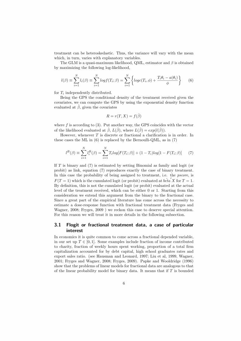
treatment can be heteroskedastic. Thus, the variance will vary with the meanwhich, in turn, varies with explanatory variables.
The GLM is a quasi-maximum likelihood, QML, estimator and β is obtainedby maximizing the following log-likelihood,
l(β) ≡
N∑
i=1
li(β) ≡
N∑
i=1
logf(Ti;β) =
N∑
i=1
{logc(Ti, φ) +
Tiθi − a(θi)
φ
}(6)
for Ti independently distributed.Being the GPS the conditional density of the treatment received given the
covariates, we can compute the GPS by using the exponential density functionevaluated at β, given the covariates
R = r(T,X) = f(β)
where f is according to (3). Put another way, the GPS coincides with the vector
of the likelihood evaluated at β, L(β), where L(β) = exp(l(β)).However, whenever T is discrete or fractional a clarification is in order. In
these cases the ML in (6) is replaced by the Bernoulli-QML, as in (7)
lB(β) ≡
N∑
i=1
lBi(β) =
N∑
i=1
Tilog[F (Ti;β)] + (1− Ti)log[1− F (Ti;β)] (7)
If T is binary and (7) is estimated by setting Binomial as family and logit (orprobit) as link, equation (7) reproduces exactly the case of binary treatment.In this case the probability of being assigned to treatment, i.e. the pscore, is
F (T = 1) which is the cumulated logit (or probit) evaluated at ˆbeta′X for T = 1.
By definition, this is not the cumulated logit (or probit) evaluated at the actuallevel of the treatment received, which can be either 0 or 1. Starting from thisconsideration we extend this argument from the binary to the fractional case.Since a great part of the empirical literature has come across the necessity toestimate a dose-response function with fractional treatment data (Fryges andWagner, 2008; Fryges, 2009 ) we reckon this case to deserve special attention.For this reason we will treat it in more details in the following subsection.
3.1 Flogit or fractional treatment data, a case of particular
interest
In economics it is quite common to come across a fractional depended variable,in our set up T ∈ [0, 1]. Some examples include fraction of income contributedto charity, fraction of weekly hours spent working, proportion of a total firmcapitalization accounted for by debt capital, high school graduates rates andexport sales ratio. (see Hausman and Leonard, 1997; Liu et al, 1999, Wagner,2001; Fryges and Wagner, 2008; Fryges, 2009). Papke and Wooldridge (1996)show that the problems of linear models for fractional data are analogous to thatof the linear probability model for binary data. It means that if T is bounded
6
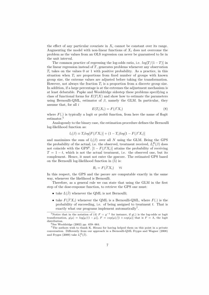
the effect of any particular covariate in Xi cannot be constant over its range.Augmenting the model with non-linear functions of Xi does not overcome theproblem as the values from an OLS regression can never be guaranteed to lie inthe unit interval.
The common practice of regressing the log-odds ratio, i.e. log[T/(1− T )] inthe linear regression instead of T , generates problems whenever any observationTi takes on the values 0 or 1 with positive probability. As a practice, in thissituation when Ti are proportions from fixed number of groups with knowngroup size, the extreme values are adjusted before taking the transformation.However, not always the fraction Ti is a proportion from a discrete group size.In addition, if a large percentage is at the extremes the adjustment mechanism isat least debatable. Papke and Wooldridge sidestep these problems specifying aclass of functional forms for E(T |X) and show how to estimate the parametersusing Bernoulli-QML, estimator of β, namely the GLM. In particular, theyassume that, for all i
E(Ti|Xi) = F (β′Xi) (8)
where F (.) is typically a logit or probit function, from here the name of flogitestimator.5
Analogously to the binary case, the estimation procedure defines the Bernoullilog-likelihood function as:
li(β) ≡ Tilog[F (β′Xi)] + (1− Ti)log[1− F (β′Xi)]
and maximizes the sum of li(β) over all N using the GLM. Being the GPSthe probability of the actual, i.e. the observed, treatment received, LB
i(β) does
not coincide with the GPS6. [1 − F (β′Xi)] attains the probability of receivingT = 1 − t, which is not the actual treatment, i.e. the observed one, but itscomplement. Hence, it must not enter the gpscore. The estimated GPS basedon the Bernoulli log-likelihood function in (5) is:
Ri = F (β′Xi) ∀i
In this respect, the GPS and the pscore are computable exactly in the sameway, whenever the likelihood is Bernoulli.
Therefore, as a general rule we can state that using the GLM in the firststep of the dose-response function, to retrieve the GPS one must:
• take L(β) whenever the QML is not Bernoulli;
• take F (β′Xi) whenever the QML is a Bernoulli-QML, where F (.) is theprobability of succeeding, i.e. of being assigned to treatment t. That isexactly what our programs implement automatically7.
5Notice that in the notation of (4) F = g−1 for instance, if g(.) is the log-odds or logittransformation, g(µ) = log[µ/(1 − µ)], F = exp(µ)/[1 + exp(µ)] that is F = Λ, the logitdistribution.
6See Wooldridge (2002) pp. 659- 664.7The authors wish to thank K. Hirano for having helped them on this point in a private
conversation. Differently from our approach in a Bernoulli-QML Fryges and Wagner (2008)
and Fryges (2009) take LBi (β).
7

4 The Estimation AlgorithmThe implementation method can be broken down into three steps. In the firststep the program gpscore2.ado estimates the GPS and tests the balancingproperties, for any family and link set. In the second step, the conditionalexpectation of the outcome is estimated as a function of the treatment level Tand the GPS R, γ(t, r) = E[Y |T = t, R = r]. Finally, in the third step thedose-response functions, ψ(t) = E[γ(t, r(t,X))], is estimated by averaging theestimated conditional expectation, γ(t, r(t,X)), over the GPS at each level ofthe treatment the user is interested in.
In detail, the first step is implemented as follows:
1. Estimate the parameters θ and φ of the selected conditional distribution ofthe treatment given the covariates. Indeed, the distribution of T is chosenfrom the exponential family through the family and link option.
2. If the family selected is Normal assess the validity of the assumed Normaldistribution model by one of the following, user-specified goodness-of-fittests: the Kolmogorov-Sminorv, the Shapiro-Francia, the Shapiro-Wilk,orthe STATA Skewness and kurtosis test for normality. The user can skipthe test through the flag b(2) option. If the Normal distribution model isstatistically disapproved, inform the user that the assumption of Normalityis not satisfied. The user is invited to use a different family and link optionor a different transformation of the treatment variable.
3. Estimate the GPS as
Ri = r(T,X) = c(T, φ)exp
{T θ − a(θ)
φ
}
where θ and φ are the estimated parameters in step 1.
4. Test the balancing property and inform the user whether and to whatextent the balancing property is supported by the data. Following Hi-rano and Imbens (2004), the program gpscore2.ado tests for balancingof covariates according to the following scheme:
a. Divide the sample in k groups according to an user-specified rule,which should be defined on the basis of the sample distribution ofthe treatment variable;
b. In the first group, k = 1, compute the GPS at the user-specifiedrepresentative point. For instance, compute the median of the groupand evaluate the GPS for each individual in the sample by settingt = median of the group;8
c. Take the GPS obtained in the previous point and divide it into nqsub-intervals defined by its quantiles of order j/nq, j = 1, . . . , nq−1.Let us call these sub-intervals as blocks;
8Notice that this will generate a distribution of the GPS with N elements for each group.
8
d. Within each block, compare individuals who are treated, i.e. belong-ing to group k (according to step a), with individuals who are in thesame block but belong to another group. Specifically, within eachblock calculate the mean difference of each covariate between unitsbelonging to group k and units not belonging to group k;
e. Combine the nq mean differences, calculated in step [d] by using aweighted average, with weights given by the number of observationsin each GPS block;
f. Go to step [b], set k = 2 and go through [b− e];
For each group tests statistics (the t-student statistics or the Bayesian-factor)are calculated and shown in the results window. Finally, the most extreme valueof the test statistics (the highest absolute value of the t-student statistics, orthe lowest value of the Bayes-factors) is compared with reference values, andthe user is informed on to what extent the balancing property is supported bythe data. If adjustment for the GPS properly balances the covariates, we wouldexpect all differences to be statistcally not significant.
Notice that for binary treatments, although the GPS is correctly calculated,the dose-response function boils down to a point rather than a curve. For thisstandard case we refer the user to pscore.ado by Becker and Ichino (2002) andto psmatch2.ado by Leuven and Sianesi (2003).9
In the second stage, the conditional expectation for the outcome Yi, givenTi and Ri, is modelled as a flexible function of its two arguments. We usepolynomial approximations of order not higher than three. Specifically, themost complex model we consider is:
ϕ(E[Yi|Ti, Ri]) = λ(Ti, Ri;α)
= α0 + α1Ti + α2T2i+ α3T
3i+ α4Ri + α5R
2i+ α6R
3i+ α7TiRi
where ϕ(.) is a function that relates the predictor, λ(Ti, Ri;α), to the conditionalexpectation E[Yi|Ti, Ri].
The last step consists of averaging the estimated regression function overthe score function evaluated at the desired level of the treatment. Specifically,in order to obtain an estimate of the entire dose-response function the programestimates the average potential outcome for each level of the treatment one isinterested in, by applying the empirical counterpart of equations (1) and (2),that is:
E[Y (t)] =1
N
N∑
i=1
γ(t, r(t,Xi)) =1
N
N∑
i=1
ϕ−1(λ(t, r(t,Xi); α))
Briefly, the program doseresponse2.ado estimates the dose-response func-tion according to the following algorithm:
9When the family is binomial the balancing mechanism is slightly different. Indeed, in thiscase the GPS is independent of t, being r(t, x) = F (β′x). Therefore, going through step [b],the algorithm will generate k times the same GPS vector. It means that step [f ] becomesineffective because the GPS does not change by changing the representative point of t.
9
1. Estimate the GPS (according to the family and link specified by the user)through the GLM approach, check the normality, if required, and test thebalancing property by using the routine gpscore2.ado.
2. Estimate the conditional expectation of the outcome, given the treatmentand the GPS, by calling the routine doseresponse_model.ado.
3. Estimate the average potential outcome for each level of the treatment theuser is interested in.
4. Estimate the standard errors of the dose-response function via bootstrap-ping10.
5. Plot of the estimated dose-response function and, if requested, its confi-dence intervals.
5 Syntax
gpscore varlist[weight
] [if
] [in
], t(varname) gpscore(newvarname)
predict(newvarname) sigma(newvarname) cutpoints(varname)
index(string) nq gps(#) family(string) link(string)[t transf(transformation) normal test(test) norm level(#)
test varlist(varlist) test(type) flag b(#) opt nb(string)
opt b(varname) detail]
doseresponse model varlist (min=2 max=2)[weight
] [if
] [in
],
outcome(varname)[cmd(regression cmd) reg type t(string)
reg type gps(string) interaction(#)]
doseresponse2 varlist[weight
] [if] [
in], outcome(varname)
t(varname) gpscore(newvarname) predict(newvarname)
sigma(newvarname) cutpoints(varname) index(string) nq gps(#)
dose response(newvarlist) family(string) link(string)[t transf(transformation) normal test(test) norm level(#)
test varlist(varlist) test(type) flag(#) cmd(regression cmd)
reg type t(string) reg type gps(string) interaction(#)
t points(vector) npoints(#) delta(#) bootstrap(string)
filename(filename) boot reps(#) analysis(string)
10As in dose-response.ado when bootstrapped standard errors are required, the bootstrapencompasses both the estimation of the GPS based on the specification given by the user, aswell as the estimation of the α parameter.
10

analysis level(#) graph(filename) flag b(#) opt nb(string)
opt b(varname) detail]
Note that in the commands gpscore2 and doseresponse2 the argumentvarlist represents the control variables, which are used to estimate the GPS.In the command doseresponse_model, varlist only consistes of two variables:the treatment variable and the GPS.
6 OptionThe doseresponse2 options include all the doseresponse options plus someothers strictly related to the GLM estimator. In what follows will be givenonly a description of the options related to doseresponse2 command, becausethey include all the options for both gpscore2 and the doseresponse_model
command. However, for each option it is reported in brackets what commandeach option is referred to.
6.1 Compulsory Options
outcome(varname) specifies that varname is the outcome variable of theprogram. [doseresponse2]
t(varname) specifies that varname is the treatment variable [gpscore2
and doseresponse2].
gpscore(newvarname) asks users to specify the variable name for the esti-mated GPS. [gpscore2]
predict(newvarname) creates a newvar to hold the maximum likelihoodestimate of the conditional standard error for the treatment given the covari-ates. [gpscore2]
sigma(newvarname) creates a newvar containing the GLM estimate of theconditional standard error of the treatment given the covariates, obtained fromPearson residuals.11 [gpscore2]
cutpoints(varname) divides the set of the potential treatment values, T ,according to the sample distribution of the treatment variable cutting at thevarname quantiles. [gpscore2]
index(string) specifies the representative point of the treatment variable atwhich the GPS has to be evaluated within each treatment interval. The argu-ment string identifies either the mean (string = mean) or a percentile (string =
11The authors wish to thank J. Wooldridge for having helped them on this point in a privateconversation. Recall that in the case on Normal distribution Pearson residuals coincide withusual residuals.
11
p1,...,p100) of the treatment.[gpscore2]
nq gps(#) specifies that the values of the GPS evaluated at representa-tive point index(string) of each treatment interval have to be divided into#(# ∈ {1, . . . , 100}) intervals, defined by the quantiles of the GPS evaluated atrepresentative point index(string).[gpscore2]
family(string) specifies the distribution family name of the treated vari-able. [gpscore2 and doseresponse2]
link(string) specifies the link function for the treated variable. The defaultis the canonical link for the family() specified.12 [gpscore2 and doseresponse2]
dose response(newvarlist) asks users to specify the variable name(s) forthe estimated dose-response function(s). [doseresponse2]
6.2 Uncompulsory Options
t transf(transformation) allows users to specify the transformation of thetreatment variable being to use in estimating the GPS. The default trans-formation is the identity function. While the supported transformations are:the logarithmic transformation, t_transf(ln); the zero-skewness log transfor-mation, t_transf(lnskew0); the Box-Cox transformation, t_transf(boxcox)and the zero-skewness Box-Cox transformation, t transf(bcskew0). The Box-Cox transformation finds the maximum likelihood estimates of the parametersof the Box-Cox transform regressing the treatment variable t(varname) on thecontrol variables listed in the input varlist.13 [gpscore2]
normal test(test) allows users to specify the goodness-of-fit test that gp-score will perform to assess the validity of the assumed Normal distributionmodel for the treatment conditional on the covariates. By default, gpscoreperforms the Kolmogorov-Smirnov test. Possible alternatives are: the Shapiro-Francia test for normality, normal_test(sfrancia); the Shapiro-Wilk test fornormality, normal_test(swilk); and the STATA Skewness and kurtosis testfor normality, normal_test(sktest). [gpscore2]
12For the list of all the possible family-link combination see table (2).13The problem is whether the treatment variable takes zero value. In such a case, the
program continues, forcing a transformation of the treatment variable to take a suitable value.Specifically, we assume that ln(0) = 0, and t transf(0) = −1/λ if λ > 0, and t transf(0) =ln(0) = 0 if λ = 0, for t transf = bcskew0, boxcox. Allowing for zero values of the treatmentimplies that untreated units might be included in the study. It should be kept in mind that theGPS score methods are designed for analyzing the effect of a treatment intensity, therefore theyspecifically refer to the subpopulation of treated units. This implies that including untreatedunits might lead to misleading results.
12
norm level(#) allows to set the significance level of the goodness-of-fit testfor normality. The default is 0.05. [gpscore2]
test varlist(varlist) specifies that the extent of covariate balancing hasto be inspected for each variable in varlist. The default test varlist consists inthe variables The order of magnitude interpretations of the Bayes Factor weapply were proposed by Jeffreys (1961). Used to estimate the GPS. This op-tion is useful when there are categorical variables among the covariates. Thecommand gpscore, which is a regression-like command, requires that categoricalvariables are expanded into indicator (also called dummy) variable sets and thatone dummy-variable set is dropped in estimating the GPS. However, the bal-ancing test should be also performed on the omitted group. This can be doneby using the option test_varlist(varlist) and by listing in varlist all thevariables, included the complete set of indicator variables for each categoricalcovariate. [gpscore2]
test(type) allows users to specify whether the balancing property has to betested using either a standard two-sides t-test (the default) or a Bayes-factorbased method test(Bayes factor). The program informs the user if there issome evidence that the balancing property is satisfied. Recall that the testis performed for each single variable in test varlist(varlist) and for eachtreatment interval. Specifically, let p be the number of control variables intest varlist(varlist), and let K be the number of the treatment intervals.We first calculate p × K values of the test statistic; then we select the worstvalue (the highest t-value in modulus, or the lowest Bayes factor) and compareit with standard values. [gpscore2]
flag b(#) skips either balancing or normal test or both, takes as arguments0; 1; 2. If not specified in the commands the program estimates the GPS per-forming both the balancing and the normal test. While if flag b(0) it skipsboth the balancing and the normal test; if flag b(1) it skips the balancing test;it flag b(2) it skips the normal test. [gpscore2]
cmd(regression cmd) defines the regression command to be used for esti-mating the conditional expectation of the outcome given the treatment and theGPS. The default cmd for the outcome variable is logit when there are two dis-tinct values, mlogit when there are 3 − 5 values, and regress otherwise. Thesupported regression commands are: logit, probit, mlogit, mprobit, ologit, opro-bit, and regress. [doseresponse_model]
reg type t(type) defines the maximum power of the treatment variable inthe polynomial function used to approximate the predictor for the conditionalexpectation of the outcome given the treatment and the GPS. The default typeis linear, meaning that the predictor λ(T, R;α) is a linear function of the treat-ment. Alternatively, type may be quadratic, or cubic. [doseresponse_model]
13
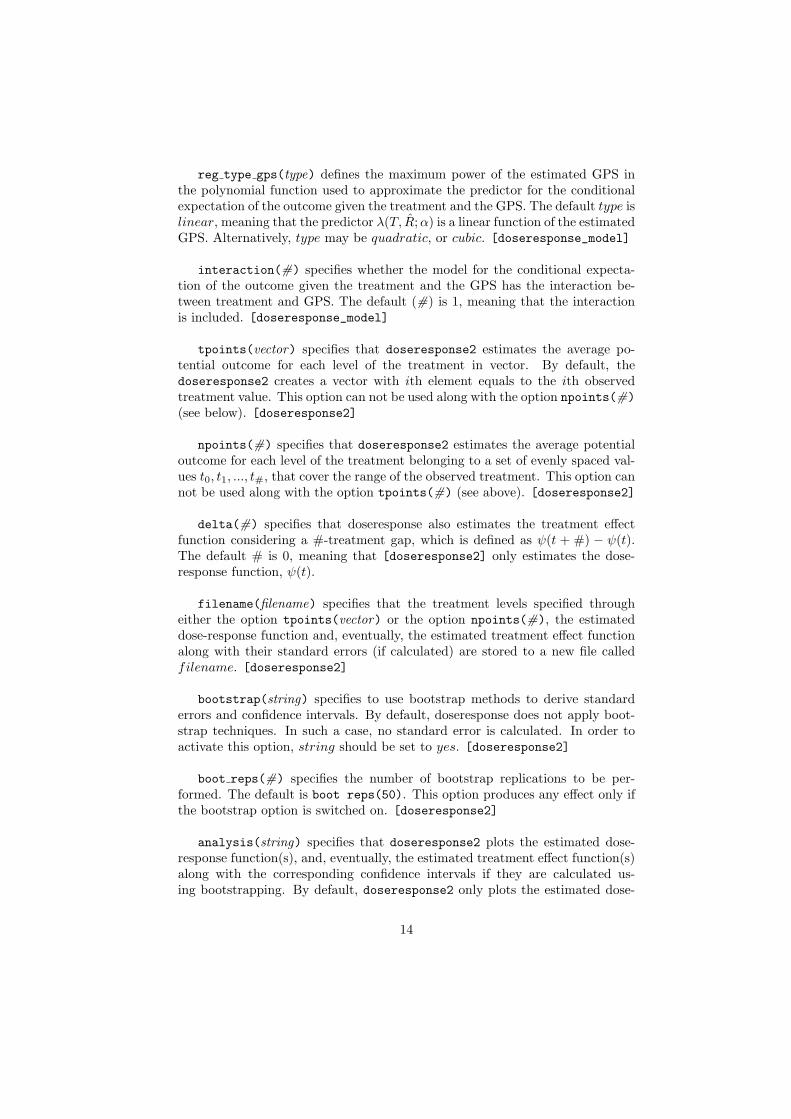
reg type gps(type) defines the maximum power of the estimated GPS inthe polynomial function used to approximate the predictor for the conditionalexpectation of the outcome given the treatment and the GPS. The default type islinear, meaning that the predictor λ(T, R;α) is a linear function of the estimatedGPS. Alternatively, type may be quadratic, or cubic. [doseresponse_model]
interaction(#) specifies whether the model for the conditional expecta-tion of the outcome given the treatment and the GPS has the interaction be-tween treatment and GPS. The default (#) is 1, meaning that the interactionis included. [doseresponse_model]
tpoints(vector) specifies that doseresponse2 estimates the average po-tential outcome for each level of the treatment in vector. By default, thedoseresponse2 creates a vector with ith element equals to the ith observedtreatment value. This option can not be used along with the option npoints(#)
(see below). [doseresponse2]
npoints(#) specifies that doseresponse2 estimates the average potentialoutcome for each level of the treatment belonging to a set of evenly spaced val-ues t0, t1, ..., t#, that cover the range of the observed treatment. This option cannot be used along with the option tpoints(#) (see above). [doseresponse2]
delta(#) specifies that doseresponse also estimates the treatment effectfunction considering a #-treatment gap, which is defined as ψ(t + #) − ψ(t).The default # is 0, meaning that [doseresponse2] only estimates the dose-response function, ψ(t).
filename(filename) specifies that the treatment levels specified througheither the option tpoints(vector) or the option npoints(#), the estimateddose-response function and, eventually, the estimated treatment effect functionalong with their standard errors (if calculated) are stored to a new file calledfilename. [doseresponse2]
bootstrap(string) specifies to use bootstrap methods to derive standarderrors and confidence intervals. By default, doseresponse does not apply boot-strap techniques. In such a case, no standard error is calculated. In order toactivate this option, string should be set to yes. [doseresponse2]
boot reps(#) specifies the number of bootstrap replications to be per-formed. The default is boot reps(50). This option produces any effect only ifthe bootstrap option is switched on. [doseresponse2]
analysis(string) specifies that doseresponse2 plots the estimated dose-response function(s), and, eventually, the estimated treatment effect function(s)along with the corresponding confidence intervals if they are calculated us-ing bootstrapping. By default, doseresponse2 only plots the estimated dose-
14
response function(s). In order to plot confidence intervals, string has to be setto yes. If the user types analysis(no), no plot is shown. [doseresponse2]
analysis level(#) allows the user to set the confidence level # of theconfidence intervals. The default confidence level is 0.95.
graph(filename) allows users to store the plots of the estimated dose-responsefunction and the estimated treatment effects to a new file called filename.When the outcome variable is categorical, doseresponse creates a new file foreach category i of the outcome variable, and names it filename i.
opt nb(string) negative binomial dispersion parameter. In the GLM ap-proach you specify fam(nb #k) where #k is specified through the option opt nb.The GLM then searches for #k that results in the deviance-based disper-sion being 1. Instead, nbreg finds the ML estimate of #k. [gpscore anddoseresponse]
opt b(varname) name of the variable which contains the number of bino-mial trials. [gpscore and doseresponse]
detail displays more detailed output. Specifically, this option allows theuser to specify that gpscore2 shows the results of the goodness-of-fit test fornormality, and some summary statistics of the distribution of the GPS evaluatedat the representative point of each treatment interval, and the results of thebalancing test within each treatment interval. When this option is specified fordoseresponse2, the results of the regression of the outcome on the treatmentand the GPS are also shown. [gpscore and doseresponse]
7 Stata outputWe illustrate the details of our programs using the dataset collected by Imbenset al (2001). In particular, the choice of the dataset has been motivated by theneed of comparison with others authors. The aim of the original exercise was toestimate the effect of the prize amount on subsequent labour earnings, “year6”.Being our econometric exercise simply motivated by the need of showing thefunctioning of the programs we have considered different treatment variables,different from “prize”, that allow us to use different family functions. In par-ticular, the flogit case has been implemented by using the treatment variable“fraction” which is obtained by normalizing the variable “prize” with respect toits highest value in the sample. Accordingly, the results of the gpscore2.ado
and of the doseresponse2.ado are shown hereafter. To show the estimationwith poisson count data we have used as a treatment variable “edu”, given bythe sum of “ownhs” and “owncoll”, namely the years of high school plus theyears of college, which, to a certain extent, can be regarded as a count variable.This exercise approximates a return to schooling estimation.
Finally, the gamma distribution is used when the treatment is “age”.
15
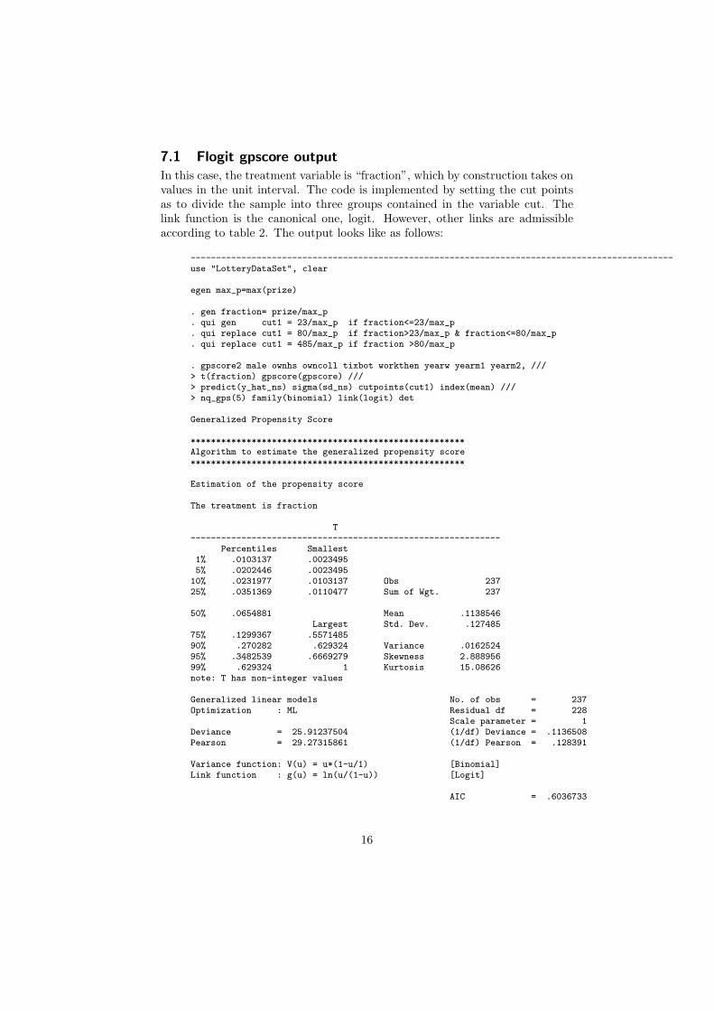
7.1 Flogit gpscore output
In this case, the treatment variable is “fraction”, which by construction takes onvalues in the unit interval. The code is implemented by setting the cut pointsas to divide the sample into three groups contained in the variable cut. Thelink function is the canonical one, logit. However, other links are admissibleaccording to table 2. The output looks like as follows:
-----------------------------------------------------------------------------------------------use "LotteryDataSet", clear
egen max_p=max(prize)
. gen fraction= prize/max_p
. qui gen cut1 = 23/max_p if fraction<=23/max_p
. qui replace cut1 = 80/max_p if fraction>23/max_p & fraction<=80/max_p
. qui replace cut1 = 485/max_p if fraction >80/max_p
. gpscore2 male ownhs owncoll tixbot workthen yearw yearm1 yearm2, ///> t(fraction) gpscore(gpscore) ///> predict(y_hat_ns) sigma(sd_ns) cutpoints(cut1) index(mean) ///> nq_gps(5) family(binomial) link(logit) det
Generalized Propensity Score
******************************************************Algorithm to estimate the generalized propensity score******************************************************
Estimation of the propensity score
The treatment is fraction
T-------------------------------------------------------------
Percentiles Smallest1% .0103137 .00234955% .0202446 .002349510% .0231977 .0103137 Obs 23725% .0351369 .0110477 Sum of Wgt. 237
50% .0654881 Mean .1138546Largest Std. Dev. .127485
75% .1299367 .557148590% .270282 .629324 Variance .016252495% .3482539 .6669279 Skewness 2.88895699% .629324 1 Kurtosis 15.08626note: T has non-integer values
Generalized linear models No. of obs = 237Optimization : ML Residual df = 228
Scale parameter = 1Deviance = 25.91237504 (1/df) Deviance = .1136508Pearson = 29.27315861 (1/df) Pearson = .128391
Variance function: V(u) = u*(1-u/1) [Binomial]Link function : g(u) = ln(u/(1-u)) [Logit]
AIC = .6036733
16
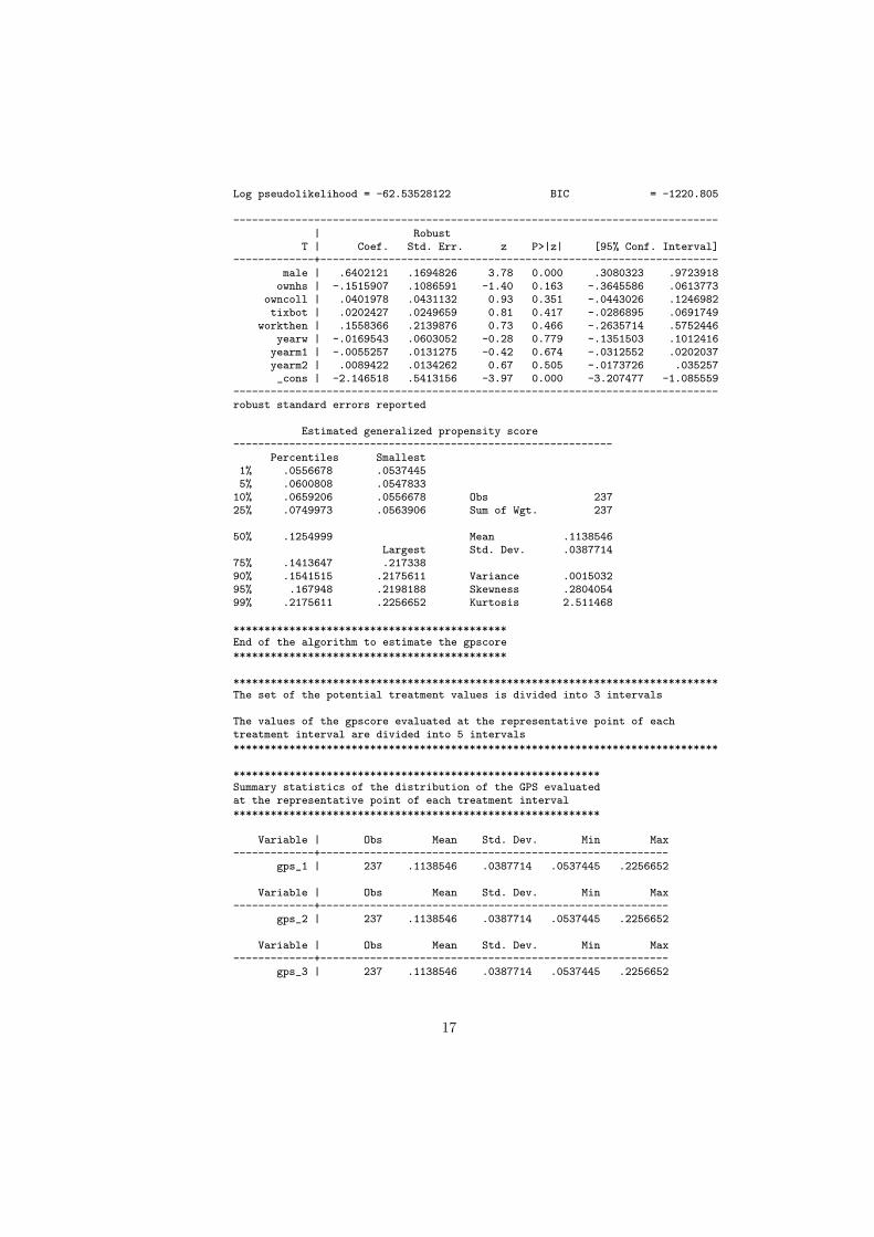
Log pseudolikelihood = -62.53528122 BIC = -1220.805
------------------------------------------------------------------------------| Robust
T | Coef. Std. Err. z P>|z| [95% Conf. Interval]-------------+----------------------------------------------------------------
male | .6402121 .1694826 3.78 0.000 .3080323 .9723918ownhs | -.1515907 .1086591 -1.40 0.163 -.3645586 .0613773
owncoll | .0401978 .0431132 0.93 0.351 -.0443026 .1246982tixbot | .0202427 .0249659 0.81 0.417 -.0286895 .0691749
workthen | .1558366 .2139876 0.73 0.466 -.2635714 .5752446yearw | -.0169543 .0603052 -0.28 0.779 -.1351503 .1012416
yearm1 | -.0055257 .0131275 -0.42 0.674 -.0312552 .0202037yearm2 | .0089422 .0134262 0.67 0.505 -.0173726 .035257_cons | -2.146518 .5413156 -3.97 0.000 -3.207477 -1.085559
------------------------------------------------------------------------------robust standard errors reported
Estimated generalized propensity score-------------------------------------------------------------
Percentiles Smallest1% .0556678 .05374455% .0600808 .054783310% .0659206 .0556678 Obs 23725% .0749973 .0563906 Sum of Wgt. 237
50% .1254999 Mean .1138546Largest Std. Dev. .0387714
75% .1413647 .21733890% .1541515 .2175611 Variance .001503295% .167948 .2198188 Skewness .280405499% .2175611 .2256652 Kurtosis 2.511468
********************************************End of the algorithm to estimate the gpscore********************************************
******************************************************************************The set of the potential treatment values is divided into 3 intervals
The values of the gpscore evaluated at the representative point of eachtreatment interval are divided into 5 intervals******************************************************************************
***********************************************************Summary statistics of the distribution of the GPS evaluatedat the representative point of each treatment interval***********************************************************
Variable | Obs Mean Std. Dev. Min Max-------------+--------------------------------------------------------
gps_1 | 237 .1138546 .0387714 .0537445 .2256652
Variable | Obs Mean Std. Dev. Min Max-------------+--------------------------------------------------------
gps_2 | 237 .1138546 .0387714 .0537445 .2256652
Variable | Obs Mean Std. Dev. Min Max-------------+--------------------------------------------------------
gps_3 | 237 .1138546 .0387714 .0537445 .2256652
17
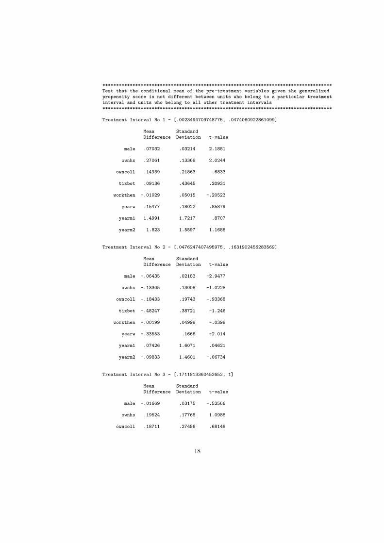
************************************************************************************Test that the conditional mean of the pre-treatment variables given the generalizedpropensity score is not different between units who belong to a particular treatmentinterval and units who belong to all other treatment intervals************************************************************************************
Treatment Interval No 1 - [.0023494709748775, .0474060922861099]
Mean StandardDifference Deviation t-value
male .07032 .03214 2.1881
ownhs .27061 .13368 2.0244
owncoll .14939 .21863 .6833
tixbot .09136 .43645 .20931
workthen -.01029 .05015 -.20523
yearw .15477 .18022 .85879
yearm1 1.4991 1.7217 .8707
yearm2 1.823 1.5597 1.1688
Treatment Interval No 2 - [.0476247407495975, .1631902456283569]
Mean StandardDifference Deviation t-value
male -.06435 .02183 -2.9477
ownhs -.13305 .13008 -1.0228
owncoll -.18433 .19743 -.93368
tixbot -.48247 .38721 -1.246
workthen -.00199 .04998 -.0398
yearw -.33553 .1666 -2.014
yearm1 .07426 1.6071 .04621
yearm2 -.09833 1.4601 -.06734
Treatment Interval No 3 - [.1711813360452652, 1]
Mean StandardDifference Deviation t-value
male -.01669 .03175 -.52566
ownhs .19524 .17768 1.0988
owncoll .18711 .27456 .68148
18
tixbot .47912 .50744 .94421
workthen -.05865 .07293 -.80421
yearw .23415 .22407 1.045
yearm1 -.70637 1.966 -.35929
yearm2 -1.1814 1.7682 -.66816
According to a standard two-sided t test:
Decisive evidence against the balancing property
The balancing property is satisfied at a level lower than 0.01
-----------------------------------------------------------------------------------------------
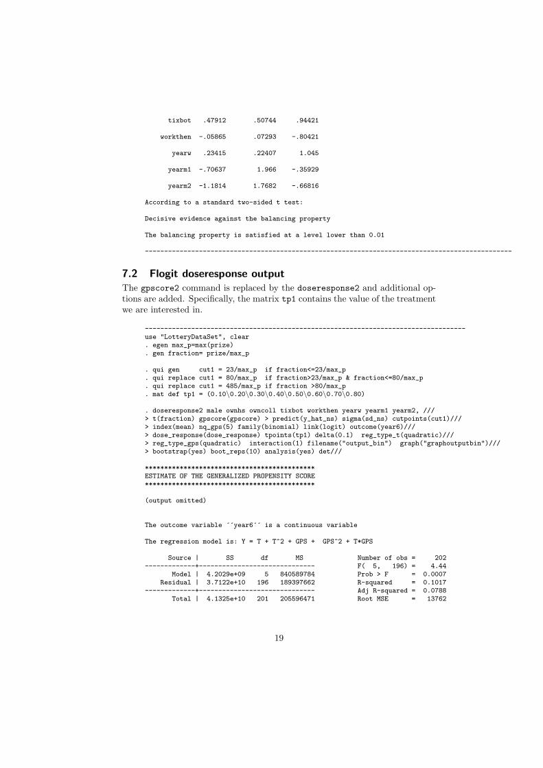
7.2 Flogit doseresponse output
The gpscore2 command is replaced by the doseresponse2 and additional op-tions are added. Specifically, the matrix tp1 contains the value of the treatmentwe are interested in.
-----------------------------------------------------------------------------------use "LotteryDataSet", clear. egen max_p=max(prize). gen fraction= prize/max_p
. qui gen cut1 = 23/max_p if fraction<=23/max_p
. qui replace cut1 = 80/max_p if fraction>23/max_p & fraction<=80/max_p
. qui replace cut1 = 485/max_p if fraction >80/max_p
. mat def tp1 = (0.10\0.20\0.30\0.40\0.50\0.60\0.70\0.80)
. doseresponse2 male ownhs owncoll tixbot workthen yearw yearm1 yearm2, ///> t(fraction) gpscore(gpscore) > predict(y_hat_ns) sigma(sd_ns) cutpoints(cut1)///> index(mean) nq_gps(5) family(binomial) link(logit) outcome(year6)///> dose_response(dose_response) tpoints(tp1) delta(0.1) reg_type_t(quadratic)///> reg_type_gps(quadratic) interaction(1) filename("output_bin") graph("graphoutputbin")///> bootstrap(yes) boot_reps(10) analysis(yes) det///
********************************************ESTIMATE OF THE GENERALIZED PROPENSITY SCORE********************************************
(output omitted)
The outcome variable ´´year6´´ is a continuous variable
The regression model is: Y = T + T^2 + GPS + GPS^2 + T*GPS
Source | SS df MS Number of obs = 202-------------+------------------------------ F( 5, 196) = 4.44
Model | 4.2029e+09 5 840589784 Prob > F = 0.0007Residual | 3.7122e+10 196 189397662 R-squared = 0.1017
-------------+------------------------------ Adj R-squared = 0.0788Total | 4.1325e+10 201 205596471 Root MSE = 13762
19
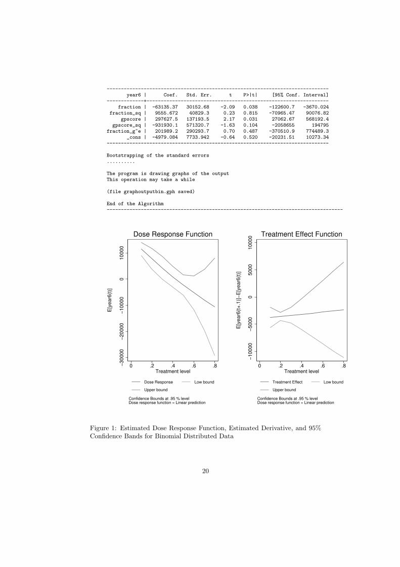
------------------------------------------------------------------------------year6 | Coef. Std. Err. t P>|t| [95% Conf. Interval]
-------------+----------------------------------------------------------------fraction | -63135.37 30152.68 -2.09 0.038 -122600.7 -3670.024
fraction_sq | 9555.672 40829.3 0.23 0.815 -70965.47 90076.82gpscore | 297627.5 137193.5 2.17 0.031 27062.67 568192.4
gpscore_sq | -931930.1 571320.7 -1.63 0.104 -2058655 194795fraction_g~e | 201989.2 290293.7 0.70 0.487 -370510.9 774489.3
_cons | -4979.084 7733.942 -0.64 0.520 -20231.51 10273.34------------------------------------------------------------------------------
Bootstrapping of the standard errors..........
The program is drawing graphs of the outputThis operation may take a while
(file graphoutputbin.gph saved)
End of the Algorithm-----------------------------------------------------------------------------------
−30000
−20000
−10000
010000
E[y
ear6
(t)]
0 .2 .4 .6 .8Treatment level
Dose Response Low bound
Upper bound
Confidence Bounds at .95 % levelDose response function = Linear prediction
Dose Response Function
−10000
−5000
05000
10000
E[y
ear6
(t+
.1)]
−E
[year6
(t)]
0 .2 .4 .6 .8Treatment level
Treatment Effect Low bound
Upper bound
Confidence Bounds at .95 % levelDose response function = Linear prediction
Treatment Effect Function
Figure 1: Estimated Dose Response Function, Estimated Derivative, and 95%Confidence Bands for Binomial Distributed Data
20
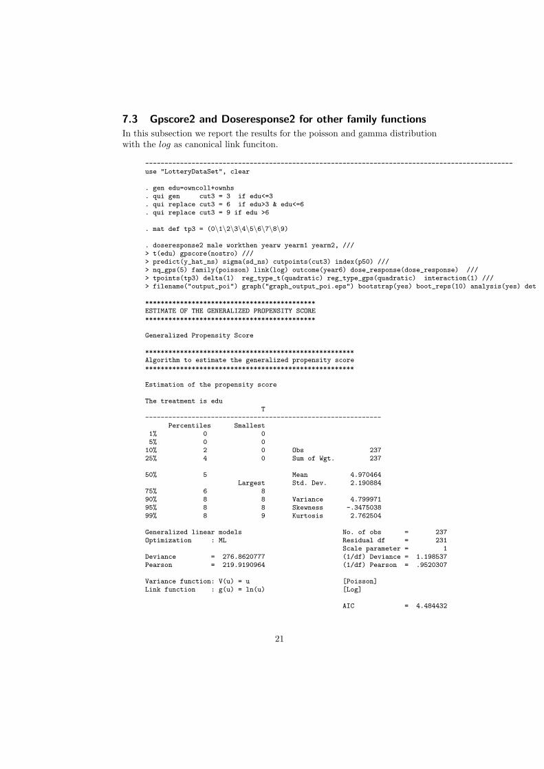
7.3 Gpscore2 and Doseresponse2 for other family functions
In this subsection we report the results for the poisson and gamma distributionwith the log as canonical link funciton.
-----------------------------------------------------------------------------------------------use "LotteryDataSet", clear
. gen edu=owncoll+ownhs
. qui gen cut3 = 3 if edu<=3
. qui replace cut3 = 6 if edu>3 & edu<=6
. qui replace cut3 = 9 if edu >6
. mat def tp3 = (0\1\2\3\4\5\6\7\8\9)
. doseresponse2 male workthen yearw yearm1 yearm2, ///> t(edu) gpscore(nostro) ///> predict(y_hat_ns) sigma(sd_ns) cutpoints(cut3) index(p50) ///> nq_gps(5) family(poisson) link(log) outcome(year6) dose_response(dose_response) ///> tpoints(tp3) delta(1) reg_type_t(quadratic) reg_type_gps(quadratic) interaction(1) ///> filename("output_poi") graph("graph_output_poi.eps") bootstrap(yes) boot_reps(10) analysis(yes) det
********************************************ESTIMATE OF THE GENERALIZED PROPENSITY SCORE********************************************
Generalized Propensity Score
******************************************************Algorithm to estimate the generalized propensity score******************************************************
Estimation of the propensity score
The treatment is eduT
-------------------------------------------------------------Percentiles Smallest
1% 0 05% 0 010% 2 0 Obs 23725% 4 0 Sum of Wgt. 237
50% 5 Mean 4.970464Largest Std. Dev. 2.190884
75% 6 890% 8 8 Variance 4.79997195% 8 8 Skewness -.347503899% 8 9 Kurtosis 2.762504
Generalized linear models No. of obs = 237Optimization : ML Residual df = 231
Scale parameter = 1Deviance = 276.8620777 (1/df) Deviance = 1.198537Pearson = 219.9190964 (1/df) Pearson = .9520307
Variance function: V(u) = u [Poisson]Link function : g(u) = ln(u) [Log]
AIC = 4.484432
21
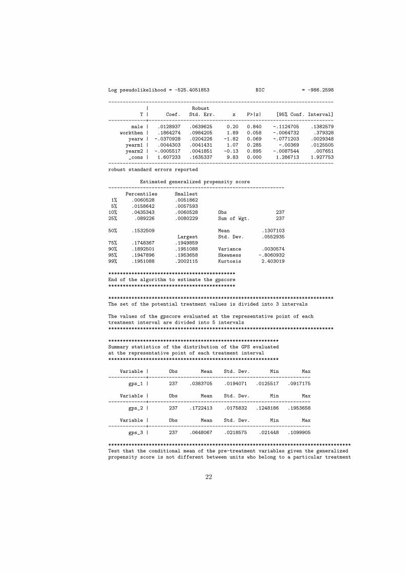
Log pseudolikelihood = -525.4051853 BIC = -986.2598
------------------------------------------------------------------------------| Robust
T | Coef. Std. Err. z P>|z| [95% Conf. Interval]-------------+----------------------------------------------------------------
male | .0128937 .0639625 0.20 0.840 -.1124705 .1382579workthen | .1864274 .0984205 1.89 0.058 -.0064732 .379328
yearw | -.0370928 .0204226 -1.82 0.069 -.0771203 .0029348yearm1 | .0044303 .0041431 1.07 0.285 -.00369 .0125505yearm2 | -.0005517 .0041851 -0.13 0.895 -.0087544 .007651_cons | 1.607233 .1635337 9.83 0.000 1.286713 1.927753
------------------------------------------------------------------------------robust standard errors reported
Estimated generalized propensity score-------------------------------------------------------------
Percentiles Smallest1% .0060528 .00518625% .0158642 .005759310% .0435343 .0060528 Obs 23725% .089226 .0080229 Sum of Wgt. 237
50% .1532509 Mean .1307103Largest Std. Dev. .0552935
75% .1748367 .194985990% .1892501 .1951088 Variance .003057495% .1947896 .1953658 Skewness -.806093299% .1951088 .2002115 Kurtosis 2.403019
********************************************End of the algorithm to estimate the gpscore********************************************
******************************************************************************The set of the potential treatment values is divided into 3 intervals
The values of the gpscore evaluated at the representative point of eachtreatment interval are divided into 5 intervals******************************************************************************
***********************************************************Summary statistics of the distribution of the GPS evaluatedat the representative point of each treatment interval***********************************************************
Variable | Obs Mean Std. Dev. Min Max-------------+--------------------------------------------------------
gps_1 | 237 .0383705 .0194071 .0125517 .0917175
Variable | Obs Mean Std. Dev. Min Max-------------+--------------------------------------------------------
gps_2 | 237 .1722413 .0175832 .1248186 .1953658
Variable | Obs Mean Std. Dev. Min Max-------------+--------------------------------------------------------
gps_3 | 237 .0648067 .0218575 .021448 .1099905
************************************************************************************Test that the conditional mean of the pre-treatment variables given the generalizedpropensity score is not different between units who belong to a particular treatment
22

interval and units who belong to all other treatment intervals************************************************************************************
Treatment Interval No 1 - [0, 3]Mean StandardDifference Deviation t-value
male -.06215 .09852 -.63091
workthen -.01101 .01395 -.78881
yearw -.32768 .2437 -1.3446
yearm1 3.4755 2.53 1.3737
yearm2 3.0207 2.5869 1.1677
Treatment Interval No 2 - [4, 6]Mean StandardDifference Deviation t-value
male .00742 .06118 .12127
workthen .00218 .02025 .10753
yearw -.22962 .138 -1.6639
yearm1 -1.5632 1.2437 -1.2569
yearm2 -1.221 1.3341 -.91525
Treatment Interval No 3 - [7, 9]Mean StandardDifference Deviation t-value
male .02225 .07089 .31384
workthen -.01708 .04406 -.38773
yearw .12469 .16353 .76246
yearm1 1.7796 1.3134 1.3549
yearm2 1.3032 1.439 .90563
According to a standard two-sided t test:Moderate evidence against the balancing propertyThe balancing property is satisfied at level 0.05The outcome variable ´´year6´´ is a continuous variableThe regression model is: Y = T + T^2 + GPS + GPS^2 + T*GPS
Source | SS df MS Number of obs = 202-------------+------------------------------ F( 5, 196) = 5.18
Model | 4.8257e+09 5 965137608 Prob > F = 0.0002Residual | 3.6499e+10 196 186220422 R-squared = 0.1168
-------------+------------------------------ Adj R-squared = 0.0942Total | 4.1325e+10 201 205596471 Root MSE = 13646
23
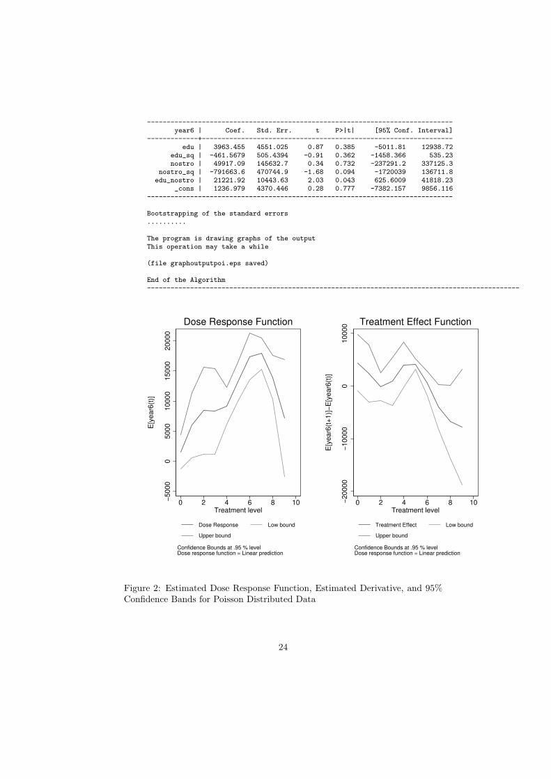
------------------------------------------------------------------------------year6 | Coef. Std. Err. t P>|t| [95% Conf. Interval]
-------------+----------------------------------------------------------------edu | 3963.455 4551.025 0.87 0.385 -5011.81 12938.72
edu_sq | -461.5679 505.4394 -0.91 0.362 -1458.366 535.23nostro | 49917.09 145632.7 0.34 0.732 -237291.2 337125.3
nostro_sq | -791663.6 470744.9 -1.68 0.094 -1720039 136711.8edu_nostro | 21221.92 10443.63 2.03 0.043 625.6009 41818.23
_cons | 1236.979 4370.446 0.28 0.777 -7382.157 9856.116------------------------------------------------------------------------------
Bootstrapping of the standard errors..........
The program is drawing graphs of the outputThis operation may take a while
(file graphoutputpoi.eps saved)
End of the Algorithm-----------------------------------------------------------------------------------------------
−5000
05000
10000
15000
20000
E[y
ear6
(t)]
0 2 4 6 8 10Treatment level
Dose Response Low bound
Upper bound
Confidence Bounds at .95 % levelDose response function = Linear prediction
Dose Response Function
−20000
−10000
010000
E[y
ear6
(t+
1)]
−E
[year6
(t)]
0 2 4 6 8 10Treatment level
Treatment Effect Low bound
Upper bound
Confidence Bounds at .95 % levelDose response function = Linear prediction
Treatment Effect Function
Figure 2: Estimated Dose Response Function, Estimated Derivative, and 95%Confidence Bands for Poisson Distributed Data
24
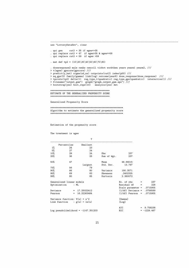
-----------------------------------------------------------------------------------------------use "LotteryDataSet", clear
. qui gen cut2 = 35 if agew<=35
. qui replace cut2 = 47 if agew>35 & agew<=59
. qui replace cut2 = 59 if agew >59
. mat def tp2 = (10\20\30\40\50\60\70\80)
. doseresponse2 male ownhs owncoll tixbot workthen yearw yearm1 yearm2, ///> t(agew) gpscore(gpscore) ///> predict(y_hat) sigma(sd_ns) cutpoints(cut2) index(p50) ///> nq_gps(5) family(gamma) link(log) outcome(year6) dose_response(dose_response) ///> tpoints(tp2) delta(1) reg_type_t(quadratic) reg_type_gps(quadratic) interaction(1) ///> filename("output_gam") graph("graph_output_gam.eps") ///> bootstrap(yes) boot_reps(10) analysis(yes) det
********************************************ESTIMATE OF THE GENERALIZED PROPENSITY SCORE********************************************
Generalized Propensity Score
******************************************************Algorithm to estimate the generalized propensity score******************************************************
Estimation of the propensity score
The treatment is agew
T-------------------------------------------------------------
Percentiles Smallest1% 24 235% 27 2410% 29 24 Obs 23725% 36 25 Sum of Wgt. 237
50% 47 Mean 46.94515Largest Std. Dev. 13.797
75% 56 7990% 66 80 Variance 190.357195% 69 83 Skewness .340232599% 80 85 Kurtosis 2.360072
Generalized linear models No. of obs = 237Optimization : ML Residual df = 228
Scale parameter = .0715905Deviance = 17.25022412 (1/df) Deviance = .0756589Pearson = 16.32263484 (1/df) Pearson = .0715905
Variance function: V(u) = u^2 [Gamma]Link function : g(u) = ln(u) [Log]
AIC = 9.758238Log pseudolikelihood = -1147.351203 BIC = -1229.467
25
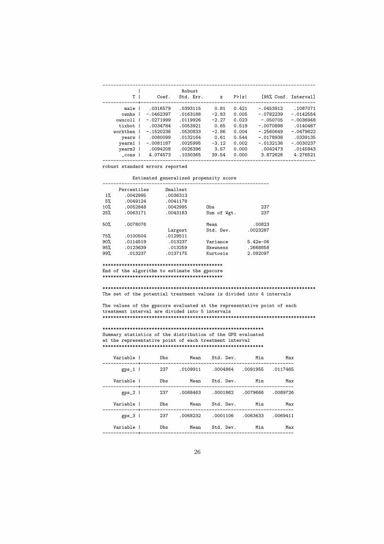
------------------------------------------------------------------------------| Robust
T | Coef. Std. Err. z P>|z| [95% Conf. Interval]-------------+----------------------------------------------------------------
male | .0316579 .0393115 0.81 0.421 -.0453912 .1087071ownhs | -.0462397 .0163188 -2.83 0.005 -.0782239 -.0142554
owncoll | -.0271999 .0119926 -2.27 0.023 -.050705 -.0036948tixbot | .0034784 .0053921 0.65 0.519 -.0070898 .0140467
workthen | -.1520236 .0530833 -2.86 0.004 -.2560649 -.0479822yearw | .0080099 .0132164 0.61 0.544 -.0178938 .0339135
yearm1 | -.0081187 .0025995 -3.12 0.002 -.0132136 -.0030237yearm2 | .0094208 .0026396 3.57 0.000 .0042473 .0145943_cons | 4.074573 .1030365 39.54 0.000 3.872626 4.276521
------------------------------------------------------------------------------robust standard errors reported
Estimated generalized propensity score-------------------------------------------------------------
Percentiles Smallest1% .0042995 .00363135% .0049124 .004117810% .0052848 .0042995 Obs 23725% .0063171 .0043183 Sum of Wgt. 237
50% .0078076 Mean .00823Largest Std. Dev. .0023287
75% .0100504 .012951190% .0114519 .013237 Variance 5.42e-0695% .0123639 .013259 Skewness .266885899% .013237 .0137175 Kurtosis 2.092097
********************************************End of the algorithm to estimate the gpscore********************************************
******************************************************************************The set of the potential treatment values is divided into 4 intervals
The values of the gpscore evaluated at the representative point of eachtreatment interval are divided into 5 intervals******************************************************************************
***********************************************************Summary statistics of the distribution of the GPS evaluatedat the representative point of each treatment interval***********************************************************
Variable | Obs Mean Std. Dev. Min Max-------------+--------------------------------------------------------
gps_1 | 237 .0109911 .0004864 .0091955 .0117465
Variable | Obs Mean Std. Dev. Min Max-------------+--------------------------------------------------------
gps_2 | 237 .0088463 .0001862 .0079666 .0089726
Variable | Obs Mean Std. Dev. Min Max-------------+--------------------------------------------------------
gps_3 | 237 .0068232 .0001106 .0063633 .0069411
Variable | Obs Mean Std. Dev. Min Max-------------+--------------------------------------------------------
26
gps_4 | 237 .0052678 .000232 .0045548 .0056592
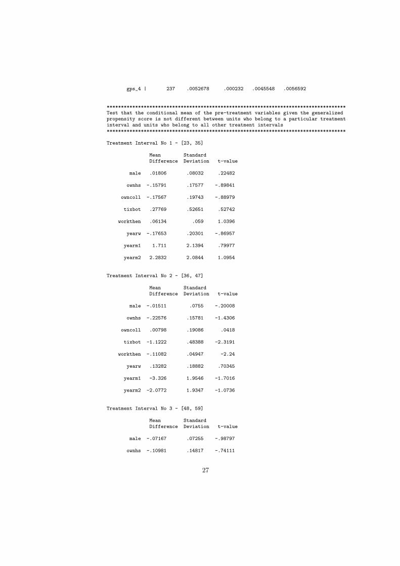
************************************************************************************Test that the conditional mean of the pre-treatment variables given the generalizedpropensity score is not different between units who belong to a particular treatmentinterval and units who belong to all other treatment intervals************************************************************************************
Treatment Interval No 1 - [23, 35]
Mean StandardDifference Deviation t-value
male .01806 .08032 .22482
ownhs -.15791 .17577 -.89841
owncoll -.17567 .19743 -.88979
tixbot .27769 .52651 .52742
workthen .06134 .059 1.0396
yearw -.17653 .20301 -.86957
yearm1 1.711 2.1394 .79977
yearm2 2.2832 2.0844 1.0954
Treatment Interval No 2 - [36, 47]
Mean StandardDifference Deviation t-value
male -.01511 .0755 -.20008
ownhs -.22576 .15781 -1.4306
owncoll .00798 .19086 .0418
tixbot -1.1222 .48388 -2.3191
workthen -.11082 .04947 -2.24
yearw .13282 .18882 .70345
yearm1 -3.326 1.9546 -1.7016
yearm2 -2.0772 1.9347 -1.0736
Treatment Interval No 3 - [48, 59]
Mean StandardDifference Deviation t-value
male -.07167 .07255 -.98797
ownhs -.10981 .14817 -.74111
27
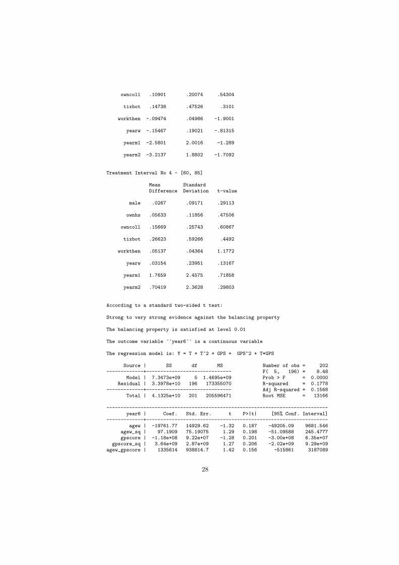
owncoll .10901 .20074 .54304
tixbot .14738 .47526 .3101
workthen -.09474 .04986 -1.9001
yearw -.15467 .19021 -.81315
yearm1 -2.5801 2.0016 -1.289
yearm2 -3.2137 1.8802 -1.7092
Treatment Interval No 4 - [60, 85]
Mean StandardDifference Deviation t-value
male .0267 .09171 .29113
ownhs .05633 .11856 .47506
owncoll .15669 .25743 .60867
tixbot .26623 .59266 .4492
workthen .05137 .04364 1.1772
yearw .03154 .23951 .13167
yearm1 1.7659 2.4575 .71858
yearm2 .70419 2.3628 .29803
According to a standard two-sided t test:
Strong to very strong evidence against the balancing property
The balancing property is satisfied at level 0.01
The outcome variable ´´year6´´ is a continuous variable
The regression model is: Y = T + T^2 + GPS + GPS^2 + T*GPS
Source | SS df MS Number of obs = 202-------------+------------------------------ F( 5, 196) = 8.48
Model | 7.3473e+09 5 1.4695e+09 Prob > F = 0.0000Residual | 3.3978e+10 196 173355070 R-squared = 0.1778
-------------+------------------------------ Adj R-squared = 0.1568Total | 4.1325e+10 201 205596471 Root MSE = 13166
------------------------------------------------------------------------------year6 | Coef. Std. Err. t P>|t| [95% Conf. Interval]
-------------+----------------------------------------------------------------agew | -19761.77 14929.62 -1.32 0.187 -49205.09 9681.546
agew_sq | 97.1909 75.19075 1.29 0.198 -51.09588 245.4777gpscore | -1.18e+08 9.22e+07 -1.28 0.201 -3.00e+08 6.35e+07
gpscore_sq | 3.64e+09 2.87e+09 1.27 0.206 -2.02e+09 9.29e+09agew_gpscore | 1335614 938814.7 1.42 0.156 -515861 3187089
28
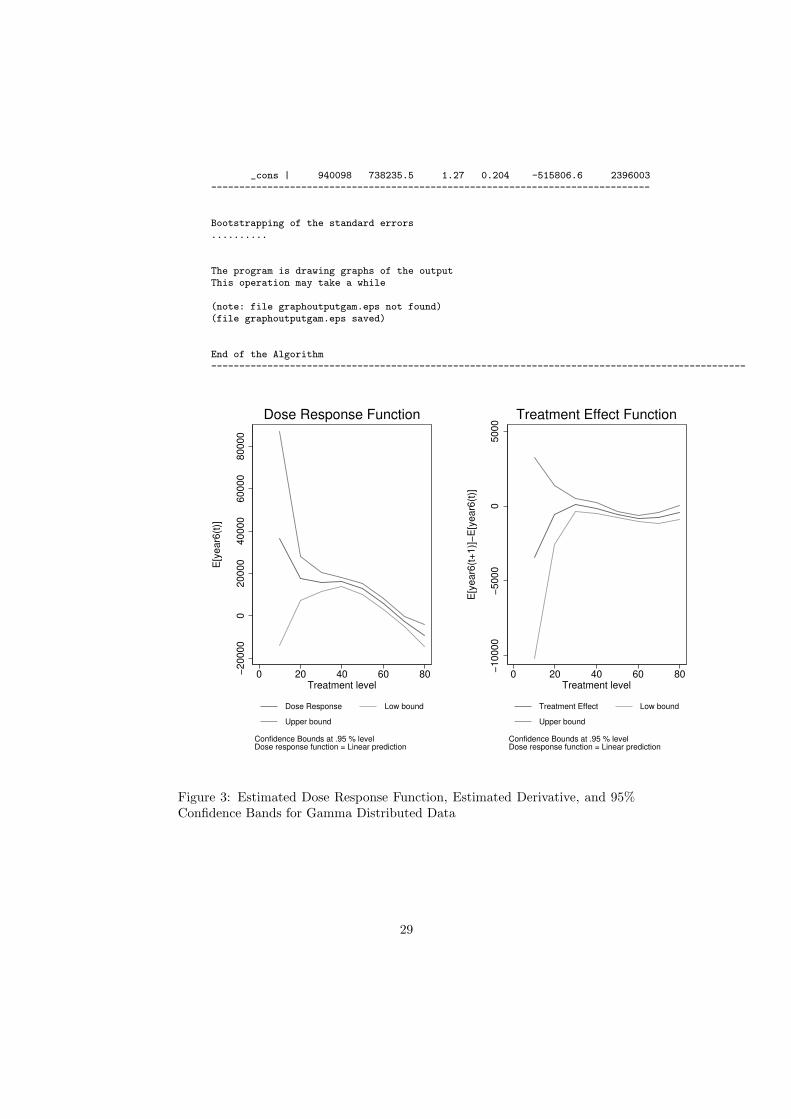
_cons | 940098 738235.5 1.27 0.204 -515806.6 2396003------------------------------------------------------------------------------
Bootstrapping of the standard errors..........
The program is drawing graphs of the outputThis operation may take a while
(note: file graphoutputgam.eps not found)(file graphoutputgam.eps saved)
End of the Algorithm-----------------------------------------------------------------------------------------------
−20000
020000
40000
60000
80000
E[y
ear6
(t)]
0 20 40 60 80Treatment level
Dose Response Low bound
Upper bound
Confidence Bounds at .95 % levelDose response function = Linear prediction
Dose Response Function
−10000
−5000
05000
E[y
ear6
(t+
1)]
−E
[year6
(t)]
0 20 40 60 80Treatment level
Treatment Effect Low bound
Upper bound
Confidence Bounds at .95 % levelDose response function = Linear prediction
Treatment Effect Function
Figure 3: Estimated Dose Response Function, Estimated Derivative, and 95%Confidence Bands for Gamma Distributed Data
29
8 ConclusionsIn recent years there is a growing interest towards the evaluation of policyinterventions and more in general towards the estimation of causal effects. Inorder to accomplish this task ad hoc softwares and programs are needed. Thepresent paper provides two STATA programs implementing the GPS in a verygeneral set up. The programs are very versatile thanks to the introduction ofthe GLM estimator in the first step of the estimation of the GPS.
AcknowledgementsThe paper benefitted from useful comments and suggestions of many people. Inparticular, the authors wish to gratefully acknowledge E. Battistin, K. Hirano,A. Mattei, J. Wooldridge. The opinions expressed by the authors are their onlyand do not necessarily reflect the position of the Institute.
9 Bibliography[1] Becker, S. O., and A. Ichino. 2002. Estimation of average treatment effects
based on propensity scores. Stata Journal 2: 358377.
[2] Bia M., and A. Mattei. 2008. A STATA package of the Estimation of theDose-Response Function through Adjustment for the Generalized PropensityScore. The Stata Journal, 8(3), 354-373.
[3] De Jong P., and G. Z. Heller. 2008. Generalized Linear Models for InsuranceData. Cambridge University press.
[4] Fryges H., and J. Wagner. 2008. Export and productivity growth: first evi-dence from a continuous treatment approach. Review of World Economics,144(4): 695-722.
[5] Fryges H. 2009. The export-growth relationship: estimating a dose-responsefunction. Applied Economics Letters, 16(18); 1855-1859.
[6] Hausman J.A., and G.K. Leonard. 1997. Superstars in the national basket-ball association: Economic value and policy. Journal of Labor Economics15, 586-624.
[7] Hirano K., and G.W. Imbens. 2004. The Propensity Score with Continu-ous Treatments. In Applied Bayesian Modeling and Causal Inference fromIncomplete-Data Perspective, ed. A. Gelman and X.-L. Meng. Whiley, 73-84.
[8] Imai K., and D.A. Van Dick. 2004. Causal inference with general treat-ment regimes: generalizing the propensity score. Journal of The AmericanStatistical Association, 99: 854-866.
[9] Imbens G.W. 2000. The role of propensity score in estimating dose-responsefunctions. Biometrika, 87: 706-710.
30
[10] Imbens G.W., D.B. Rubin, and B. Sacerdote. 2001. Estimating the effectof unearned income on labor supply, earnings, savings and consumption:evidence from a survey of lottery players. American Economic Review, 91:778-794.
[11] Lechner M.R. 2001. Identification and estimation of causal effects of mul-tiple treatments under the conditional independence assumption, in Econo-metric Evaluation of Labour Market Policies, M. Lechner and F. Pfeiffereds, Physica, Heidelberg.
[12] Leuven, E., and B. Sianesi. 2003. psmatch2: Stata module to per-form full Mahalanobis and propensity score matching, common sup-port graphing, and covariate imbalance testing. Boston College Depart-ment of Economics, Statistical Software Components. Downloadable fromhttp://ideas.repec.org/c/boc/bocode/s432001.html.
[13] Liu J.L., J.T. Liu, J.K. Hammitt, and S.Y Chou. 1999. The price elasticityof opium in Taiwan, 1914-1942. Journal of Health Economics 18; 795-810.
[14] McCullagh P., and J.A. Nelder. 1989. Generalized Linear Models. Secondedition. New York: Chapman and Hall.
[15] Papke L.E. and J.M. Wooldridge. 1996. Econometric Methods for fractionalresponse variables with an application to 401 (K) plan Participation rates.Journal of Applied Econometrics, 11(6): 619-632
[16] Rabe-Hesketh S. and B. Everitt. 2000. A handbook of Statistical Analysesusing Stata. Second Eds, Chapman & Hall/Crc. Boca Raton London NewYork Washington D.C..
[17] Rosenbaum P.R., and D.B. Rubin. 1983. The central role of the propensityscore in observational studies for causal inference. Biometrika 70: 41-55.
[18] Rosenbaum P.R., and D.B. Rubin. 1984. Reducing bias in observationalstudies using classification on the propensity score. Journal of The Ameri-can Statistical Association, 73, 516-24.
[19] Wagner J. 2001. A note on the firm size-export relationship. Small BusinessEconomics 17, 229-337.
[20] Wooldridge J.M.. 2002. Econometric analysis of cross section and paneldata. MIT Press.
31