Essays on Financial Information Analysis - Project...

Essays on Financial Information Analysis

by

Harm Schuett

A dissertation submitted in partial satisfaction of the

requirements for the degree of

Doctor of Philosophy

in

Business Administration

in the

Graduate Division

of the

University of California, Berkeley

Committee in charge:

Patricia Dechow, ChairSunil DuttaRichard Sloan

Stefano DellaVigna

Spring 2013


Copyright 2013by

Harm Schuett

1

Abstract


by

Harm Schuett

Doctor of Philosophy in Business Administration

University of California, Berkeley

Patricia Dechow, Chair

How can accounting be useful to investors and facilitate equity valuation? In thedissertation at hand, I provide three essays that add to the literature about earningsquality and financial analysis.

The first chapter provides a framework for the three studies that comprise chapter2 to 4. I discuss the normative principles that underlie the valuation of an equitystake in a company as advocated by Penman (2010) and as taught in most MBAcourses. I proceed to derive a proposition that useful accounting minimizes investors’forecast errors of abnormal earnings over the life of the firm. This demand forms thebasis on which I will judge and test the usefulness of several accounting methods forvaluation throughout the dissertation.

The second chapter is titled “The Matching Principle: Timely Information to In-vestors?” In it, I empirically test whether and how the matching principle (matchingexpenses to revenues) provides investors with more timely information. I hypothe-size and find empirical evidence that matching provides investors with an accountingmargin and rate of return that is a more informative and less noisy anchor for fore-casting a firm’s future business performance. Changes in accounting margins basedon adequately matched expenses are a timelier signal of changes in underlying busi-ness performance.

In the third chapter, “Does Matching Expenses to Revenues Increase the Useful-ness of Fundamental Signals?”, I examine whether fundamental accounting signalsare more insightful the more expenses are matched to revenues. This chapter adds tothe literature by comprehensively examining how matching of expenses to revenuesimproves or weakens the predictive ability of financial signals for future earnings.Second, I investigate whether market participants react differently to financials sig-nals from firms with a high degree of matched expenses compared to signals from

2

firms with a low degree of matched expenses. The results indicate that the degree ofmatched expenses significantly and positively affects the predictive power of account-ing based signals (signals that are based on accounting mechanics such as abnormalinventory growth). On the other hand, the predictive ability of “non-accounting”signals such as abnormal capex growth diminishes. Furthermore, the relation be-tween matching and the predictive power of the signals is driven at least as muchby accounting choices as the underlying business factors. At the same time, thereis only weak evidence that market participants such as analysts reacts differently tofundamental signals for high-matching firms. Analyst forecast revisions only showa weakly increasing relation between signals and revisions. In contrast, there is arobust increasing relation between forecast errors and signals.

The fourth chapter is titled “Do Analysts Understand the Relation Between In-vestment Intensity and Earnings Growth?” The aim of this chapter is to test whetherthe accounting for investments is understood by valuation experts such as analysts.I identify a transitory pattern in earnings growth that is caused by changes in afirm’s investment activity and whose magnitude depends on the degree of conser-vative accounting used for these investments. Since, the pattern is mechanical andcan be predicted, I test whether analysts do so. I provide evidence that they do notfully anticipate transitory changes in earnings growth and that these cases result inabnormal returns around subsequent earnings announcements.

i

Dedication

For my Mum and Dad with their endless love and support over the years. For mybrothers, who always keep me sane and on my toes. For my love Larissa.

ii

Contents

Contents ii

List of Figures iv

List of Tables iv

1 Accounting, Financial Information Analysis and Equity Investors 11.1 Introduction . . . . . . . . . . . . . . . . . . . . . . . . . . . . . . . . 11.2 A Model of Valuation . . . . . . . . . . . . . . . . . . . . . . . . . . . 21.3 Conclusion . . . . . . . . . . . . . . . . . . . . . . . . . . . . . . . . . 7

2 The Matching Principle: Timely Information to Investors? 82.1 Introduction . . . . . . . . . . . . . . . . . . . . . . . . . . . . . . . . 92.2 Literature Review . . . . . . . . . . . . . . . . . . . . . . . . . . . . . 112.3 Theory: The Matching Concept and Accounting Rates of Return . . 132.4 Hypotheses: The Link Between Matched Expenses and Earnings’ Use-

fulness . . . . . . . . . . . . . . . . . . . . . . . . . . . . . . . . . . . 192.5 Empirical Results . . . . . . . . . . . . . . . . . . . . . . . . . . . . . 202.6 Conclusion . . . . . . . . . . . . . . . . . . . . . . . . . . . . . . . . . 26

3 Does Matching Expenses to Revenues Increase the Usefulness ofFundamental Signals? 273.1 Introduction . . . . . . . . . . . . . . . . . . . . . . . . . . . . . . . . 273.2 Prediction and Research Design . . . . . . . . . . . . . . . . . . . . . 283.3 Empirical Analysis . . . . . . . . . . . . . . . . . . . . . . . . . . . . 333.4 Results . . . . . . . . . . . . . . . . . . . . . . . . . . . . . . . . . . . 343.5 Conclusion . . . . . . . . . . . . . . . . . . . . . . . . . . . . . . . . . 38

4 Do Analysts Understand the Relation Between Investment Inten-sity and Earnings Growth? 40

iii

4.1 Introduction . . . . . . . . . . . . . . . . . . . . . . . . . . . . . . . . 414.2 Literature Review . . . . . . . . . . . . . . . . . . . . . . . . . . . . . 434.3 The Joint Effect of Accounting Conservatism and Investment Growth 454.4 Hypotheses . . . . . . . . . . . . . . . . . . . . . . . . . . . . . . . . 474.5 Empirical Results . . . . . . . . . . . . . . . . . . . . . . . . . . . . . 504.6 Conclusion . . . . . . . . . . . . . . . . . . . . . . . . . . . . . . . . . 59

Bibliography 61

A Appendix: Variable Definitions 69

B Appendix: Proofs 74B.1 Danielson and Press (2003) Proof for IRR Formula . . . . . . . . . . 74B.2 Proof for Investment Intensity Model Equations . . . . . . . . . . . . 75

C Appendix: Figures and Tables 78C.1 Chapter 2 Tables . . . . . . . . . . . . . . . . . . . . . . . . . . . . . 78C.2 Chapter 3 Tables . . . . . . . . . . . . . . . . . . . . . . . . . . . . . 90C.3 Chapter 4 Figures and Tables . . . . . . . . . . . . . . . . . . . . . . 101

iv

List of Figures

1 Directional Prediction of the Investment Intensity Effect on Changes inEarnings Growth. . . . . . . . . . . . . . . . . . . . . . . . . . . . . . . . 48

2 Computation of Consensus Forecasts . . . . . . . . . . . . . . . . . . . . 49

3 Investment Growth vs. Selected Variables for Highest IG Quintile insideHighest Conservatism Quintile . . . . . . . . . . . . . . . . . . . . . . . 101

4 △ Investment Intensity vs Investment Growth for Highest △II Quintileinside Highest Conservatism Quintile . . . . . . . . . . . . . . . . . . . . 102

List of Tables

1 Definitions of IRR Estimation Variables (see McNichols, Rajan, and Re-ichelstein (2012)) . . . . . . . . . . . . . . . . . . . . . . . . . . . . . . . 69

2 Definitions of Matching Proxy Test Variables . . . . . . . . . . . . . . . . 703 Definitions of Investment Intensity Test Variables . . . . . . . . . . . . . 714 Definitions of Fundamental Signal Variables . . . . . . . . . . . . . . . . 73

5 Illustration of Distortions in the Accounting Rate of Return . . . . . . . 796 Descriptive Statistics for the Base Sample . . . . . . . . . . . . . . . . . 817 Distribution of the Matching Proxy by Industry . . . . . . . . . . . . . . 828 Correlation Matrix of Selected Variables . . . . . . . . . . . . . . . . . . 839 Means of Selected Variables ranked by Matching Portfolios . . . . . . . . 8410 Descriptive Statistics for Selected Conservatism Correction Variables . . 85

v

11 Correlation Matrix for Selected Conservatism Correction Variables . . . . 8612 EBV/ABV by Matching Rank . . . . . . . . . . . . . . . . . . . . . . . . 8713 ARR-IRR by Matching Rank . . . . . . . . . . . . . . . . . . . . . . . . 8814 FERC Regressions by Matching Portfolio . . . . . . . . . . . . . . . . . . 8915 Descriptive Statistics for Model Variables . . . . . . . . . . . . . . . . . . 9015 Distribution of INV for each MATCH Quintile . . . . . . . . . . . . . . 9016 Correlation Matrix for Model Variables . . . . . . . . . . . . . . . . . . . 9117 Updating Abarbanell and Bushee (1997) Tests . . . . . . . . . . . . . . . 9218 Portfolio Regression of Fundamental Signals on Changes in Earnings Growth 9319 Portfolio Regression of Fundamental Signals on Forecast Revisions . . . . 9420 Portfolio Regression of Fundamental Signals on Forecast Errors . . . . . 9521 Portfolio Regression of Fundamental Signals on Contemporaneous Returns 9622 Portfolio Regression of Fundamental Signals on Future Returns . . . . . 9723 Industry-adjusted Portfolio Regressions of Fundamental Signals . . . . . 9824 Numerical Example Illustrating Accounting Distortions . . . . . . . . . . 10325 Descriptive Statistics for Model Variables . . . . . . . . . . . . . . . . . . 10426 Correlation Matrix for Model Variables . . . . . . . . . . . . . . . . . . . 10527 Pearson Correlations by Average Past Conservatism Quintile . . . . . . . 10628 Portfolio Regression on Changes in Earnings Growth . . . . . . . . . . . 10729 Regression on Changes in Earnings Growth . . . . . . . . . . . . . . . . 10830 Portfolio Regression on Changes in Earnings Growth for High and Low

Variance Firms . . . . . . . . . . . . . . . . . . . . . . . . . . . . . . . . 10931 Portfolio Regression on Analyst Forecast Errors . . . . . . . . . . . . . . 11032 Regression on Analyst Forecast Errors . . . . . . . . . . . . . . . . . . . 11133 Portfolio Regression on Analyst Forecast Revisions . . . . . . . . . . . . 11234 Hedging Portfolio Returns . . . . . . . . . . . . . . . . . . . . . . . . . . 11335 Portfolio Regression on Analyst Sales Forecast Errors . . . . . . . . . . . 11536 Portfolio Regression on Analyst Pre-Tax Forecast Errors . . . . . . . . . 116

vi

Acknowledgments

I thank the members of my dissertation committee: Patricia Dechow, Sunil Dutta,Richard Sloan, and Stefano DellaVigna for their time and guidance. In additionI thank Brian Ayash, Panos Patatoukas, Alexander Nezlobin, Xiao-Jun Zhang andThorsten Sellhorn for their assistance and many helpful comments and the Center forFinancial Reporting and Management (CFRM) for financial support. I also thankthe participants in research workshops at the Haas School of Business, University ofGraz and WHU Vallendar for their helpful comments. All errors are my own.

1

Chapter 1

Accounting, Financial InformationAnalysis and Equity Investors

1.1 Introduction

What kind of accounting is useful to investors and for what reason? The FASB’sintermediate answer to the first question is: accounting that helps investors valuethe stock of a company. ”The objective of general purpose financial reporting is toprovide financial information about the reporting entity that is useful to existing andpotential investors, lenders, and other creditors in making decisions about providingresources to the entity. Those decisions involve buying, selling, or holding equity anddebt instruments and providing or settling loans and other forms of credit” (SFACNo. 8 2010, OB2)1

Unfortunately, up to this date, the answer to the follow up question ”what kind ofaccounting is useful for valuation?” depends on a normative model of how to handlethe accounting for equity valuation. That is because, the question ”how shouldinvestors go about valuation?” remains normative at its core. This is unsatisfying formodern researchers, who will try their best to avoid normative questions (Friedman(1966)). Nevertheless, until accounting researchers have successfully teamed up withbehavioral psychologists and derived a valuation model that optimizes valuationperformance subject to our information processing constraints, researchers will haveto rely on ”common sense” principles of valuation.

1In the obsolete SFAC 1, this statement was stronger and more precise: ”financial statementsshould help investors and creditors in “assessing the amounts, timing, and uncertainty” of futurecash flows” (FASB 1978).

2

First, one has to agree on how investors ”should” go about equity valuation.More precisely, one first needs to agree on the optimal method for valuation beforewe can start to research what accounting system best supports this valuation method.Valuation methods are basically a set of techniques for determining the value of afirm’s shares. As Penman writes: “Valuation methods are utilitarian – they serveto guide practice – so the choice between competing technologies ultimately comesdown to how useful they are for the practical task of evaluating investments.” (p1.Penman (2005)). So, asking how investors should go about equity valuation is asking:What is the best practical method? Which valuation method guides investors bestthrough financial statement analysis and the forecasting process? Only then can onefind answers to the question of how accounting can facilitate the valuation process;one can discuss whether conservatism and matching are helpful accounting concepts,or whether fair value accounting is useful to investors. As it turns out, separatingvaluation from accounting is not as easy as it sounds. In his book ”Accounting forValue”, Penman (2010) goes even further and argues that valuation is accounting forvalue and therefore accounting and valuation are the same thing. Here is why.

1.2 A Model of Valuation

The basis for any valuation model is the discounted cash flow model, first formallyexpressed by I. Fisher (1930) and Williams (1938):

FVt = Et[∞∑

k=1

CFt+k

(1 + r)k], (1.1)

where FVt is the fair value of the equity, CFt is the cash flow going to equity investors,and r is the cost of equity capital.

An asset’s value is equal to the future cash flows it generates to its owner, dis-counted by the expected return. Thus, valuation is essentially forecasting futurecash flows. This is by no means an easy task. A firm potentially lives forever. Ascountless stories in the Wall street journal show, it is often difficult to predict howa firm will fare one year from now, let alone ten years. Business conditions changefast, competition is ever reshuffling the cards of the game and the global economypresents investors with countless variables to forecast. A good valuation methodshould facilitate this daunting task. The optimal valuation model (with the helpof accounting) will minimize investors’ forecast errors of the present value of futurecash flows, subject to constraints by investors’ information processing mechanisms

3

and the cost of information gathering.2

The role of accounting in this endeavor can be made clear by reformulating thediscounted cash flow model. Although it is technically feasible to forecast futurecash flows directly, it is hardly the most efficient. In practice, investors usually firstforecast key financial statement metrics. Only in a second step do they translatethem into cash flow forecasts.

The residual income model was introduced into the American business world byEdwards and Bell (1961), K. Peasnell (1982), and Ohlson (1995). It is now advocatedin many text books (see for instance Lundholm and Sloan (2012), Penman (2012)and Easton et al. (2013)) because it uses financials directly to derive a firm’s value.

FVt = BVt + Et[∞∑

k=1

Earnt+k − r ∗BVt+k−1

(1 + r)k], (1.2)

where Earnt is a firm’s earnings and BVt is a firm’s book value of equity.A firm’s value is its book value plus the present value of its expected future

abnormal earnings. Assuming that clean surplus accounting is used, the residualincome model is a direct transformation of the discounted cash flow model. No otherassumptions about accounting are need. This is simultaneously an advantage anda caveat. The residual income method works with any arbitrary accounting systemas long as it follows clean surplus accounting.3 Consider cash accounting. All cashoutflows are immediately expensed and inflows are booked when received. Bookvalue is then zero and the residual income model is equal to the discounted cash flowmodel.

While the RIM stresses Penman’s point that valuation is essentially an accountingproblem, it does not seem to help us in deciding what kind of accounting is useful toinvestors. We merely substituted the minimization problem from minimizing fore-cast errors of future cash flows to minimizing forecast errors of future abnormalearnings. Even worse, abnormal earnings are a vacuous statistic. Its interpretationand meaning depends crucially on the underlying accounting. Abnormal earningsunder fair value accounting have a vastly different interpretation (with different fore-casting properties) than abnormal earnings under historical cost accounting and yet

2Assumptions about investors information processing capabilities also define what level of cap-ital market efficiency is assumed. If one assumes completely efficient markets, then there are nogains to be had from financial information analysis. If all information is already baked into theprice, then accounting is irrelevant. However, then it becomes hard to see how the informationenters the price. Realistically our information processing capability is limited and accounting isrelevant for investors.

3Clean surplus accounting simply means that all changes in the balance sheet unrelated todividends must run through the income statement.

4

another interpretation under replacement cost accounting. However, concluding thatforecasting earnings is useless – or accounting does not matter – would be hasty.

(Lee (1999), p.3) states that the “essential task in valuation is forecasting. It isthe forecast that breathes life into a valuation model”. In the spirit of Lee (1999),I argue that useful accounting is that which infuses abnormal earnings with such aninterpretation as that earnings become the easiest to forecast over the whole life of thefirm. The qualifier ”over the whole life of the firm” is critically important. Imagine anaccounting system that smooths earnings to such an extreme that abnormal earningshave been constant in the past, even though the business was volatile. Then earningsseem to be perfectly predictable. However, such abnormal earnings would have noeconomic meaning. Moreover, it is impossible to smooth earnings forever. At somepoint the accounting has to reverse and this will eventually reveal the underlyingeconomic situation of the business. These reversals will be hard to predict and leadto large forecast errors. Such abnormal earnings would also yield no indication asto what the terminal value at the end of the forecast horizon should be. The call tominimize forecast errors has to include the forecasts made to arrive at the terminalvalue.

Charging accounting with minimizing investors’ forecast errors of abnormal earn-ings over the whole life of the firm gives us a better handle on how to improvevaluation outcomes by pinning down appropriate accounting rules. For instance, themost speculative task in valuation is to forecast the terminal value of a valuationmodel. Indeed, Penman (2005) argues that “accounting must be evaluated on howit deals with the truncation problem” (Penman (2005),p.369). The terminal valueis the present value of all future cash flows after a certain period (usually ten to 20years) under the assumption of a stable growth rate. To avoid forecasting a terminalvalue altogether, it would make sense to set abnormal earnings at the end of theforecast horizon equal to zero.4 This can be done in a simple way that yet has anintuitive economic interpretation. Basic economic forces demand that a firm in acompetitive market only earns an economic rate of return equal to its cost of capital.For any firm in a competitive market, the difference between the economic rate ofreturn and the firm’s cost of capital must be zero in the long run. Therefore, oneway of setting abnormal earnings to zero in the long run is to account for a firm’sbusiness in such a way that the accounting rate of return is equal to its economicrate of return. Then the accounting rate of return will equal the firm’s cost of capitalin the terminal period, abnormal earnings will be zero. The forecasting process thenbecomes an exercise in estimating a firm’s sales growth and its decline in competi-

4Remember, setting long run abnormal earnings to zero is a simple matter of accounting andwon’t affect the underlying value.

5

tive advantage relative to its competitors, taking a big chunk of speculation out ofthe forecasting process. Chapter 2 will go into details about the merits and difficul-ties of this particular approach of setting the accounting rate of return equal to theeconomic rate of return.5

Making accounting reflect a firm’s current competitive situation as close as pos-sible also agrees with the principles used by Penman (2010) to arrive at accountingfor value. He uses what he calls the ten fundamental principles to derive his valua-tion and accounting model. These principles have their origin in Graham and Dodd(1996) and are in ascending sequence (Penman (2010), p.6)

1. One does not buy a stock, one buys a company.

2. When buying a business, know the business.

3. Price is what you pay, value is what you get.

4. Part of the risk of investing is the risk of paying too much.

5. Ignore information at your peril.

6. Understand what you know and don’t mix what you know with speculation.

7. Anchor your valuation on what you know rather than on speculation.

8. Beware of paying too much for growth.

9. When calculating value to challenge the price, don’t put price into the calcu-lation.

10. Return to fundamentals; prices gravitate to fundamentals.

From these principles he derives the following key demands of accounting.

1. Valuation is translating ones’ knowledge about the business and its executioninto price. Translating is a matter of accounting. Accounting needs to focusthe lens on the business model.

5This view is related to but not the same as forecasting sustainable earnings or earnings per-sistence. Assessing earnings persistence is another form of earnings forecasting. Using currentearnings as a benchmark, it is analyzed whether future earnings will continue to follow the sametrend (See Lintner and Glauber (1967) and Ball and Watts (1972)).

6

2. Leave speculation to the investor. Investing critically involves speculatingabout the future. Speculation is necessary. But it needs to be guided asbest as possible. Accounting needs to provide an anchor to keep speculation incheck.

3. Accounting should protect from paying too much for growth.

4. Information should be independent of price. Accounting needs to be able tochallenge the price.

5. Especially true for growth. Accounting must be credible information so thatfundamental value gets ultimately revealed to the market.

6. Valuation as ”What will the financials look like in three to five years”.

Penman’s demands agree to a large extent with my proposition that accountingshould minimize the forecast errors of abnormal earnings over the whole life spanof the firm. “Accounting needs to focus the lens on the business” equals the claimthat accounting should reflect the underlying economics of the business and fosterforecasting of its competitive situation. The same goes for the demand to leavespeculation to investors. If the accounting depicts as reliable and precise an image ofthe current competitive situation as possible, then this will anchor speculation aboutthe competitive situation in the future. It is hard to be overly optimistic about afirm’s future performance if you have a clear picture of the competition it faces.

Penman’s demands further contain two strong arguments for conservative ac-counting and against fair value accounting. Fair value accounting, the practice ofbooking an asset at its explicit market value or hypothetical selling price, would in-troduce market prices into the financial statements. Penman argues that this wouldimpede accounting’s ability to challenge the market price of a company. (Penman(2010), pp.169-174) To be fair to standard setters, such fair value inputs have to belabeled according to how speculative they are. Whether they are observed on liquidmarkets, or derived from a model. But, as history has shown, even liquid markets candetach from fundamentals temporarily. The argument is valid that such deviationsare what investors are eager to analyze and challenge. Therefore they should not bepart of the financial statements. Again this works with the proposition to minimizeinvestors’ forecast errors.

Penman’s case for conservatism is that it keeps speculation out of the financialstatements. Assets should only be recognized if they are reasonably certain (or asPenman (2010) puts it, have become a low beta asset (Penman (2010), pp.156-158).However, applying the forecast minimization objective, it is not quite clear whether

7

the demand for conservatism is as unequivocally intuitive as is the case of fair valueaccounting. Conservatism throws sand into the mapping of economic rates of returninto accounting rates of return. Chapter 2 and 4 will provide evidence of the detri-mental effects of conservative accounting to investors. There is a trade-off betweenaccounting reflecting the competitive situation of a firm adequately and leaving anykind of speculation out of the financials. A case in point is that valuation for researchand development investments. Under US-GAAP no asset is recognized for researchand development investments. This accounting is conservative. The rationale for thistreatment is that future benefits from research and development are uncertain andtoo hard to quantify. Recognizing them as an asset would put too much speculationinto financials. The case is well made. On the other hand, as will be shown in chapter2 to 4, this conservative treatment distorts the picture that accounting paints of afirm’s business. Rates of return differ from the underlying economic rate of returnand earnings growth changes do not necessarily reflect changes in investment growthor profitability any more. Matching expenses to revenues, or even replacement costaccounting, remedies this distortion but require estimation of an asset’s useful lifeand future benefits. A trade-off has to be made.

1.3 Conclusion

The preceding discussion provided a framework on which accounting’s usefulness forinvestors can be measured. However it is necessarily normative to some extent. Inwhat follows, I will try to provide more details and empirical evidence for investors,researchers and regulators on the consequences of matching expenses to revenues andthe consequences of conservative accounting.

8

Chapter 2

The Matching Principle: TimelyInformation to Investors?

Abstract: This chapter examines whether matching expenses to revenues increasesearnings’ usefulness to investors by providing an accounting rate of return (ARR)closer to current economic profitability. To test this, I estimate a proxy for a firm’sinternal rate of return (IRR) in order to approximate the distortion between ARRand IRR. Results show that the magnitude of the difference is reduced for firmswith a higher degree of matched expenses. The median magnitude is 1.4% for thehighest matching quintile, suggesting that matching expenses provides a reasonableproxy for economic profitability. Secondly, it is argued that reducing the gap betweenARR and IRR leads to more timely information included in current earnings. Thisis evidenced by firms with a smaller gap between ARR and IRR and higher degreesof matched expenses exhibiting a higher return reaction to current earnings (ERC)and a lower return relation with future earnings (FERC).

9

2.1 Introduction

Economists and Accounting academics alike have often advocated that a firm’s ac-counting must be informative about a firm’s current underlying economic profitabilityin order to be useful in measuring profitability, pricing shares or assessing manage-rial performance (K. V. Peasnell (1996) or Danielson and Press (2003)). However,while it is easy to see why a better measure of current economic performance leadsto a more accurate assessment of managerial performance, the link between currentperformance and its importance in valuing a company is less clear. After all it isfuture profitability not current profitability that matters for valuation. To be helpfulfor valuation, earnings information must be timely. This study aims to contribute tothe debate by empirically testing (1) how well accounting numbers reflect economicprofitability in the cross-section and (2) whether a close approximation is associatedwith more timely value relevant information.

Especially in the industrial organization literature economic return is often usedsynonymously with the internal rate of return on a firm’s investment (Fisher andMcGowan (1983)). Early theoretical work has shown that the only accounting thatequates ARR and IRR is neutral accounting (Solomon (1966); Hotelling (1925)).Even full matching of expenses does not generally equal neutral accounting (Rajan,Reichelstein, and Soliman (2007). Therefore, it is of great interest to regulators,academics and practitioners alike to get an estimate of the magnitude of divergencebetween accounting rates of return and economic profitability and its correlation withthe timeliness of earnings information. This is the main motivation of the paper.

This study fits into the literature about accounting rates of return as a measureof economic profitability (Fisher and McGowan (1983)) as well as the classic earningsquality literature on what accounting rules best reflect sustainable and value relevantearnings (Penman and Zhang (2002)). My contribution to this literature is twofold:First, I empirically measure the link between the accounting principle of matchingexpenses to revenues1 with the economic property of providing a closer approxima-tion of the current economic rate of return. The economic rate of return is herebydefined as the internal rate of return on a firm’s current projects.2 To achieve this,

1Formulated in the matching principle which was formerly part of the US-GAAP and IFRSframework. See IFRS Framework, point 95 and the FASB Concepts Statement No. 8. See alsoMadray (2008) for an overview.

2The IRR is not undisputed as a yardstick. For instance, Vatter (1966) contests that sincethe IRR is an average rate over the whole term of an investment, it is not a good measure ofeconomic profitability in a particular period. A related concept is economic income and one wouldbe tempted to rephrase the above question into whether accounting income approximates economicincome. However there exist numerous definitions of ”economic income”. For instance Feltham

10

two new empirical constructs, matching precision as well as an alternative IRR es-timator, are introduced. With these I examine the magnitude of divergence betweenARR and IRR for different degrees of matched expenses, testing how well matchingfulfills the economist’s demand for a measure of economic profitability.3 Secondly, Itest if a closer approximation of the current economic rate of return of a firms in-vestments provides more timely and value relevant information for projecting futurerates of return. Earnings timeliness is defined here as in Collins et al. (1994):”Withits emphasis on historical-cost measurement and transaction-based accounting, theconventional accrual model often trades off timeliness in recognizing changes in netasset values in favor of objectivity, verifiability, and/or conservatism.”(p.292).4 Moretimely earnings provide users of accounting data faster with decision useful informa-tion. Thus in my tests for valuation implications, I focus on this aspect of earningsquality; as the lack of timeliness is one of the most commonly mentioned shortcom-ings of conventional historical cost accounting.

I draw on prior results and methods by Danielson and Press (2003) and McNi-chols, Rajan, and Reichelstein (2012) to develop the estimator for IRR. Danielsonand Press (2003) use a simple model relating ARR and IRR via past growth ininvestment and the ratio of economic book value to accounting book value. Theyuse the market-to-book ratio to put an upper bound on the ratio of economic toaccounting book value and estimate bounds for the IRR for a sample of steady statefirms. In contrast, I use the market-to-book decomposition by McNichols, Rajan,and Reichelstein (2012) to estimate the ratio of economic to accounting book valuedirectly and am therefore able to compute a estimate of IRR rather than puttingbounds on a possible range. Second, I develop a measure for the degree of matched

and Ohlson (1996) test under which situation accounting income is equal to economic income. Thisis only vaguely related to the analysis in this paper however since Feltham and Ohlson examine”‘Hicksian”’ economic income, which is essentially changes in firm value during the observed period.In contrast, the economic income definition that equates ARR and IRR used by Hotelling (1925)is more akin to Pareto’s original concept, using the IRR as discount rate rather than the costof capital. Therefore, throughout the paper, I tried to avoid the term economic income to avoidconfusion.

3The accounting rate of return meant here is the equivalent of return on invested capital. Ichose to refer to it as accounting rate of return to emphasize the very nature of this rate of returnas an accounting approximation of an underlying performance concept

4The notion of timeliness used here is the following. Earnings are timely if they signal persistentchanges in future performance. This is closely connected to the concept of earnings power byGraham and Dodd (1996). It is therefore slightly different, but not inconsistent with the notionused for instance in Basu (1997). For example, in the framework of this paper, a write-down canbe viewed as a correction of previous bad matching; of assets that have an inflated book value. Thewrite-down itself is therefore not timely, but the new margin and rate of return after the write-downwill provide a better picture of current and future profitability, which is timely information.

11

expenses (MATCH), which is based on the Predicted R-squared of a regression ofchanges in expenses on changes in revenues. With this I test the following hypothe-ses: H1 says that matching expenses to revenues provides a close approximation ofthe internal rate of return. The magnitude of the gap between ARR and IRR hasa negative and monotonic relation to the degree of matching. Theoretical resultsby Stauffer (1971) and the empirical results by Danielson and Press (2003) providethe motivation for this claim. Second, earnings numbers that closely approximateeconomic profits provide margins and accounting rates of return that only vary withchanges in the underlying IRR of a firm’s projects. In contrast, deviations suchas conservative or aggressive accounting will introduce more transitory noise intomargins and returns.5 H2 states that, since changes in margins and rates of returnare more likely due to changes of underlying profitability, earnings of firms witha high degree of matched expenses are also more timely, i.e. provide more timelyinformation about future earnings.

Results are consistent with these hypotheses. The difference between ARR andIRR (hereafter called the ARR − IRR gap) has an inverse, monotonic relationshipwith the degree of matching. The gap varies from 5% points for the lowest expensematching precision quintile to 1.4% for the highest quintile. Tests to validate the mea-sures show that matching precision is significantly related to RNOA and operatingmargin variance, as well as plausible firm characteristics such as intangible intensity,PP&E intensity or persistence. Linking matching expenses to the ARR − IRR gapand the gap to earnings timeliness further shows that earnings are also more timely.This is evidenced by higher ERCs while having lower FERCs for firms with a higherdegree of matching.

The paper proceeds as follows. Section 2.2 reviews the literature, Section 2.3discusses the concepts behind the matching principle and provides the theory and anexample for the link between matching precision and the difference between ARR andIRR. Section 2.4 formulates the hypotheses and section 2.5 contains the empiricaltests. Section 2.6 concludes.

2.2 Literature Review

Academic discussions regarding the appropriateness of the matching principle startedwith the seminal monograph of Paton and Littleton (1940), who coined the termexpense ”matching” and elevated it to the backbone of sound accounting practices.

5See for instance Penman and Zhang (2002) and Feltham and Ohlson (1996). I define conser-vative and aggressive accounting with respect to the benchmark of economic depreciation, called”neutral accounting.

12

The comment by Wilcox (1941) is an early source of criticism of the Paton andLittleton (1940) view of universal importance of the matching principle. Brief andOwen (1969), Brief and Owen (1970) and Jarrett (1971) are the first to pose thematching problem as an estimation problem of a performance measure when facedwith uncertain cash flows and a fixed time horizon.

Among papers explicitly examining the matching relationship, the recent paperby Dichev and Tang (2008), draws a persuasive connection between the correlationbetween revenues and expenses on the one hand and the variability of earnings on theother. The authors argue that the economy’s shift from a manufacturing and tradeeconomy towards a service and intellectual property economy, as well as the FASB’sparadigm shift towards a more balance sheet focused fair value accounting, led toa decline in the matching relation, which in turn led to a deterioration of earningsquality (operationalized by earnings volatility).6 Follow-up research tries to shedfurther light on the reasons for this decline. Donelson, Jennings, and McInnis (2011)argue that this shift is almost entirely due to an increase in the incidence of largespecial items, which they attribute to changes in the economic environment ratherthan changes in the accounting environment.7 Prakash and Sinha (2010) investigatehow revenue deferrals in combination with indirect costs and immediate expensingof investment expenditures can exacerbate the mismatch in the timing of revenueand expense recognition. The study at hand adds to this stream of the earningsquality literature by examining the connection between the matching of expenses torevenues and timeliness of earnings.

The paper is also closely connected to the theoretical debate about the useful-ness of accounting rates of returns in the economics literature and the problems inestimating a firm’s economic rate of return. This debate reaches back to Hotelling(1925) who coins the term economic depreciation for that depreciation schedule,which equates the accounting rate of return to the internal rate of return and setsthis schedule as the benchmark. Motivated by the question of how to regulate mo-nopolies, Fisher and McGowan (1983); F. M. Fisher (1988); Salamon (1985, 1988)argue that accounting rates of return are a poor proxy for economic rates of return(See K. V. Peasnell (1996) for a review). They argue that the accounting systemshould be measured on how closely the accounting rate of return ARR representsthe economic rate of return, which Fisher and McGowan (1983) set equal to the

6Dechow 1994 also argues that the negative correlation between accruals and cash flows is dueto matching.

7Dichev and Tang (2008) also acknowledge the effect of one-time items but caution that elim-inating those would ”throw out the baby with the bathwater”. For the purposes of this paper– assessing the economic importance of well-matched earnings irrespective of the cause of badmatching – this point is of secondary importance.

13

internal rate of return (IRR). On closer inspection however, it becomes clear thatthis demand would do injustice to accountants. Apart from the practical problemsin measuring IRR, one has to be careful with the notion of IRR one is interested in.This is highlighted by Demsetz (1997). As cited by K. V. Peasnell (1996): ”The rateof return on an investment can never be known, even in principle, until a projectends. The concept of the economic rate of return, as used by Fisher and McGowan,is therefore not very useful for determining how things are progressing in a worldfull of uncertainty and in which investment projects are being allowed to continue.”(Demsetz 1995, p. 98).

Demsetz correctly points out that in reality the IRR can not be known in advanceand consequently accounting rates can also only be an approximation of what isinherently unknown until completion. Fisher and McGowan (1983) argue that theonly thing, one can say for certain about the location of the economic rate of return isthatARR and IRR are on the same side of the growth rate. Stewart III. (1991) in theclassic book on EVA calculation also discuss IRR estimation but acknowledges theimprecise nature of the estimates. Steele (1986) advocates an approach to estimatingIRR from financial statements which proves equally restricted. Danielson and Press(2003), by bringing in the accounting implications of conservative accounting, showthat one can say much more about the ARR− IRR gap and frequently put a rangeon it. In their study however they only look at steady firms but find that a firm’sARR is often a useful starting point for evaluating a firm’s IRR. Rajan, Reichelstein,and Soliman (2007) provides a detailed treatment of the effects of conservatism andgrowth on return on capital invested and consequently about the difference betweenARR and IRR. However for their purposes, they do not need a measure of IRR. Icontribute to this stream of literature by proposing a workable solution for researchersto approximate the difference between ARR and IRR based on a method used byMcNichols, Rajan, and Reichelstein (2012) to decompose the market-to-book ratioand simulation results by Rajan and Reichelstein (2009).

2.3 Theory: The Matching Concept and

Accounting Rates of Return

The Connection between Matching Expenses and Revenuesand Earnings Timeliness

The purpose of matching expenses to revenues is to provide an accurate picture ofthe profitability of a firm’s current transactions with its customers (sales) (Paton and

14

Littleton (1940)). It is therefore backward-looking information and can only providevalue relevant information (that is info about future performance), if there is a linkbetween current and future profitability.

Few will argue that in the real world a firm’s current and future profitability areunrelated. In reality, the cut between past and the future is not as dramatic as itseems. Many firms engage in similar activities over time, and changes in activitiesand market conditions are rarely so drastic as to render past activities completelyirrelevant for forecasting future activities. Therefore, the role of past earnings as arepresentative starting point for future expectations should not be underestimated.Matching expenses to revenues should strengthen this link between current and futureearnings by providing a reasonably accurate picture of economic profitability. Themore closely accounting rates of return resemble economic rates of return, the lessearnings are plagued by transitory distortions in profitability such as the ones causedby conservative accounting (Penman and Zhang (2002), Rajan, Reichelstein, andSoliman (2007) and Richardson et al. (2006)). Instead, changes in profitability andmargins will mainly be due to changes in underlying economics.

Table 5 illustrates conservatism mechanics That can lead to such distortions andreduce the timeliness of earnings. These are the same mechanics as examined byPenman and Zhang (2002). While they are consequences for earnings sustainability,I stress the additional consequences for earnings timeliness. A firm is drawn thatinvests repeatedly in the same project. In some of the years the amount investedgrows but the investment opportunity with an IRR of 28.9% stays the same. Thisis done to highlight the fact that growth does in fact not necessarily distort margins.For each $1 invested in period t, the firm earns $0.75 in t+1, $0.5 in t+2 and $0.35in t + 3. The first case is the perfect matching case. Here the investment costs areamortized in accordance with the revenue stream over the next three periods (50%in t+ 1, 33% in t+ 2 and 17% in t+ 3). In the second case, 40% of the investmentamount is expensed immediately. The remaining 60% are then amortized accordingto the revenues stream. In both cases the underlying profitability of the operation isthe same (IRR of 28.9%). But, as one can see by comparing the accounting rate ofreturn and margin, shown each period in case one versus case two, matched earningsprovide a more reliable and accurate time series of returns and margins than the caseof direct expensing.8 The observable distortions in the rate of return and marginsresulting from reversals of directly expensed investments in conjunction with chang-ing growth rates have been widely discussed in Rajan, Reichelstein, and Soliman

8The example also shows that matching affects the denominator of the accounting rate of returnas well as asset turnovers. Incorporating the two effects into the discussion might yield strongerhypothesis and I plan to do so soon.

15

(2007), Penman and Zhang (2002) and Richardson et al. (2006). In this example,accelerating investment growth in conjunction with unconditional conservatism (di-rect expensing of 40% of the costs) lead to a build up in hidden reserves, depressingearnings. The deceleration in investment growth later on releases the reserves, in-creasing earnings. The example illustrates the timely nature of information underperfect matching. changes in profitability and margins occur fast and only because ofchanges in underlying economics. Therefore, if the current projects are still contin-uing and provide a good starting point for the investment opportunities that a firmfaces in the near future, we are given a helpful picture of the firm’s future earningspower. Earnings are more sustainable and indicative of future performance.

Measuring ˆIRR and Expense Matching

However, ARR does not equal IRR even under fully matched expenses. Hotelling(1925) shows that ARR only equals IRR when the book value of assets is equal topresent value of future cash flow from historic investments, discounted using the finalIRR. He calls this the economic book value (EBV ) and the change in EBV economicdepreciation.9 A more elaborate proof can be found in Stauffer (1971) with the sameconclusion that the two are only equal if “the depreciation schedule ... is defined asthe time-rate-of-change of the present value of the cash flow stream” (p467 Stauffer(1971)). This is also commonly called “neutral” or “unbiased” accounting (Rajan,Reichelstein, and Soliman (2007). The complexity of the derivation in Stauffer (1971)is not necessary for the analysis in this paper. For the sake of brevity, I will brieflyintroduce the more parsimonious model by Danielson and Press (2003) to motivatethe construction of my measure of ˆIRR.

The model is based on 5 assumptions: (1) A firm’s new investments can containtangible and intangible investments with the ratio staying the same, (2) each newunit of investment produces cash inflows over the following N periods, (3) the firmdoes not change its accounting methods, (4) each cohort of assets wears out at thesame rate over N periods, but might have different profitability and (4) the firm hasa constant historic growth rate.10 With these assumptions the following equationcan be deduced quite easily (the proof by Danielson and Press (2003) can be found

9Hotelling (1925) assumed zero NPV projects when deriving his mathematical theory of de-preciation. Under this assumption, economic depreciation (or neutral depreciation) also equals therelative practical capacity (RPC) depreciation rule (see Rajan and Reichelstein (2009)).

10These assumptions are similar to assumptions used in Fisher and McGowan (1983), Rajan,Reichelstein, and Soliman (2007) or Stauffer (1971).

16

in appendix B).

ARR = (IRR− g) ∗ EBV

ABV+ g (2.1)

Equation 2.1 explains accounting rates of return (ARR) as a function of the inter-nal rate of return, growth in assets and the difference between economic book value(EBV ) and accounting book value (ABV ) (equation 3 on p.497 in Danielson andPress (2003))11. Equation (2.1) captures our intuition from table 5. The key driver isthe difference between economic book value (EBV ) and GAAP book value (ABV ),with growth in assets (g) mediating the distortion. Intuitively, the ratio reflects theamount of hidden reserves not on a firm’s balance sheet. Rajan, Reichelstein, andSoliman (2007) show that (1) higher growth leads to lower return on investment inthe presence of conservatism and (2) that more conservative accounting increasesRoIC, if growth has been moderate, and decreases RoIC, when growth has beenhigh. To build an estimator of IRR, we can rearrange equation 2.1 to get IRR as afunction of ARR, the ratio of EBV/ABV and growth g.

IRR = ARR + (g − ARR) ∗ (1− ABV

EBV) (2.2)

Although g is assumed to be constant over the firm’s investment history in theoriginal model by Danielson and Press (2003), they show that reasonable approx-imations are not too noisy. For instance, they show via simulations that the lossof accuracy using the geometric mean over the prior 3 years as growth rate inputdoes not add too much noise (increases the standard deviation by 10%). The keyto get an accurate estimator of IRR is therefore to find an efficient way to esti-mate ABV/EBV . McNichols, Rajan, and Reichelstein (2012) develop an estima-tion procedure for this ratio in order to estimate the proportion of conservatism inthe market-to-book ratio. They call EBV/ABV the conservatism correction factor(CCF ). I will use versions of their measures in my empirical tests to estimate theratio of ABV/EBV and consequently the difference between ARR and IRR.

McNichols, Rajan, and Reichelstein (2012) call the ratio EBV/ABV the conser-vatism correction factor and (CCF ). However, one important difference is that theirnotion of economic book value is based on replacement costs, whereas the one usedhere is based on historical capital invested (and not used up yet). They assume aone horse shay scenario for asset productivity12 and apply the annuity depreciation

11This equation can be found in various varieties across the literature. See Rajan, Reichelstein,and Soliman (2007); Skogsvik (1998); Ohlson and Gao (2006)

12Meaning that assets provide the same capacity each period until the end of their useful life atwhich point the capacity abruptly is zero.

17

method to compute the proxies. In a competitive market where IRR equals the costof capital replacement cost accounting and neutral accounting will coincide. Howeverthis would also imply economic rents for the firm being zero. Under the assumptionthat assets decline equally over time, the annuity depreciation method at the heart ofthese proxies coincides with neutral accounting again though. This assumption seemsnot restrictive, especially for intangible assets such as R&D.13 Furthermore, simula-tions by Rajan and Reichelstein (2009) show that accounting margins do not differtoo much from replacement cost accounting, as long as there is not direct epxensingof investments. I therefore use their measures as proxies to compute EBV/ABV .The first measure capitalizes an estimate of economic rents ( ˆV ER). The estimate ofV ERt

ABVt(V ERB or VER-to-book-value) is computed by computing a measure of eco-

nomic cost of the current period that is based on the annuity depreciation method.The estimate of economic rent is computed by extrapolating these costs proxies intothe future (See McNichols, Rajan, and Reichelstein (2012)).14 I call the resultingestimate the V ER conservatism correction factor ( ˆCCFV ER). For comparison pur-poses I also use two direct methods by McNichols, Rajan, and Reichelstein (2012)to estimate the ratio EBV/ABV . ˆCCF and ˆCCF3 estimate EBV/ABV directlyvia estimating the useful life of a firm’s current capital investments and then cap-italizing and depreciating past investments according to the annuity depreciationmethod. The only difference is that ˆCCF uses actual historic year-over-year growthin investment over the estimated useful live of a firm’s current assets for estimation,whereas ˆCCF3 uses the geometric mean over the past 3 years as an approximation.15

The next tool needed for the empirical tests is a measure of the degree of matchingin a firm’s accounting system. Dichev and Tang (2008) proxy for the degree ofmatching using the partial correlation between revenues and expenses for rolling 5year windows for each year of a sample of the 100 largest firms in that year. Theirchoice is strongly influenced by their focus on the changing properties of matchingover time. The focus of this paper however is on the general determinants of matchingand its implications, warranting a different test design. For one thing, computing the

13For instance Noland (2011) points out that firms use the sum-of-the-years digit method todepreciate intangible assets such as customer relationships, reflecting the fast decline in usefulnessof these types of assets.

14As McNichols, Rajan, and Reichelstein (2012) argue, this approach is broadly in the spirit ofNezlobin (2012) using the average growth rate over the past years to proxy for anticipated futuregrowth.

15The full model and derivation by McNichols, Rajan, and Reichelstein (2012) is quite involvedand will not be repeated here for the sake of keeping the study compact (the exact empiricalcomputation can be found in the appendix). An assumption underlying all measures is that capitalinvestments are the only source of accruals. While this is clearly unrealistic, it is of no great concernfor the study of expense matching, since current assets are comparably easy to match to revenues.

18

correlation between revenues and expenses for each firm on rolling windows resultsin a correlation measure with very low variability. Low variability makes it difficultto disentangle actual variation from noise. Equally important is that revenues andexpenses are trending variables for most windows. This can create a spurious relationand artificially create very high correlation measures if used in pooled samples.

△Expensei,t = α0 + α1 ∗ △Revenuei,t + ei,t (2.3)

To overcome these issues, I use the Predicted R-squared of regression (2.3).Whereas the normal R-squared indicates how well the model fits the data, the Pre-dicted R-squared indicates how well the model predicts responses to new observa-tions and was first proposed by Allen (1974). It is an indicator of the predictiveability of revenues for expenses. Computing it is straightforward. Forecast errorsare estimated by systematically removing each observation from the firm time-series,estimating regression coefficients without it and then testing how well the modelpredicts the removed observation. The error between the prediction and the actualremoved value is used to compute the Predicted R-squared. Equations (2.4) comparecomputations for the normal R-squared and Predicted R-squared.

R2 = 1− SSResid

SSTot

= 1−∑

i(yi − yi)∑

i(yi − y)(2.4)

R2Pred. = 1− SSPredicted

SSTot

= 1−∑

i(yi − ˆyi,−i)∑

i(yi − y)

, where ˆyi,−i is the out-of-sample fitted value of yi.The rationale is that if a company is able to match expenses to revenues well,

knowing revenues should enable the market to predict expenses better. The PredictedR-squared presents itself as a natural measure for this predictive ability. I use changesin revenues and expenses in order to get rid of the spurious relation introduced bypossible trends and rolling 8 year windows for each firm in the sample. Although8 years of past data make for a small time-series, it is more than what one finds inmost analyst reports and therefore appears to be a reasonable upper bound as to thenumber of past years examined by most investors.

High values of the Predicted R-squared from regression (2.3) indicate that changesin revenues were a good predictor of changes in expenses during the 5 years exam-ined. The maximum value of 1, for instance, would indicate a constant growth inmargin during those 8 years – changes in expenses were perfectly linearly projectedby changes in revenues. Low values indicate the opposite; changes in revenues haveonly a weak predictive ability for expenses, indicating that only few of the period’sexpenses were matched to the period’s revenues. The lowest values are likely due to

19

large one-time write-offs, which, Dichev and Tang (2008) suggest, are a manifestationof previously erroneous matching reversing.

2.4 Hypotheses: The Link Between Matched

Expenses and Earnings’ Usefulness

Matching and the Difference Between ARR and IRR

Even under perfect matching precision, ARR is not equal to IRR. But (as illustratedin table 5) more conservative or aggressive accounting leads to even bigger distortionsover the growth cycle of a firm through either understated assets (a smaller ratio ofaccounting book value of assets to economic value of assets (ABV/EBV )), in thecase of conservative accounting, or overstated assets (a higher ratio of ABV/EBV ),in the case of aggressive accounting. Coming from either side, we expect ABV/EBVto approach 1 as the amount o matched expenses increases. Consequently ARR −IRR will decrease, holding growth fixed (See equation (2.2)). Since conservativeaccounting is much more prevalent, for instance due to the direct expensing of R&D,it is more likely that an increase in matching would lead to an increase in ABV/EBV .But no matter whether the starting point is, conservative or aggressive accounting,an increase in matching should lead to a monotonic decrease in the magnitude of theARR− IRR gap. The first sub hypotheses are therefore:

H1(A): Firms with a higher amount of matched expenses have on averageABV/EBVratios closer to one.

H1(B): Due to the prevalence of conservative elements, the average correlationbetween matching and EBV/ABV is negative.

H1(C): The relation between matching and ARR−IRR is monotonically decreasingceteris paribus.

where ABV is the accounting book value of capital invested and EBV is theeconomic book value of capital invested.

The Degree of Expense Matching and Timeliness

However, even under perfect matching precision, historic cost accounting still onlyprovides information about past events and investments. Also, predictability doesnot imply timely information. Earnings can theoretically be completely predictable –

20

for instance be constant over time – and not provide any useful information to valuea firm. I hypothesize that the higher predictability of future earnings, caused bythe lack of noise from accounting distortions, also leads to more timely information.Consider the example in table 5 again. In the perfect matching accounting case,any margin change will signal a change in economic profitability, irrespective of thecurrent and past growth rate. In the conservative accounting case on the other hand,economic profitability measures are camouflaged by accounting distortions.

To test the hypothesis, I use a setup similar to the one developed by Collinset al. (1994) and used by Gelb and Zarowin (2002). They regress returns on currentand future unexpected earnings. Timeliness is proxied by the coefficient, or ERC, ofcurrent earnings. The ERC captures the information content in current earnings thatis also in current returns. Similarly if earnings are timely, returns should not varymuch with future earnings as this would imply stale information in earnings. This iscaptured by the coefficients on future unexpected earnings, or FERC. More timelyearnings should therefore have higher ERCs and lower FERCs. Taken together H2

can be written as:

H2: Earnings from a stronger matching relation provide on average more timelyinformation as evidenced by higher ERCs and lower FERCs, ceteris paribus.

where ERC is the coefficient of regressing current unexpected earnings on con-temporaneous earnings and FERC is the sum of the coefficients of regressing futureunexpected earnings over the next three years on contemporaneous earnings.

2.5 Empirical Results

Data and Sample Construction

The empirical tests in this paper utilize data from the Compustat Annual NorthAmerica file from 1975 till 2007 and the CRSP monthly stock returns file. Firms inthese three databases were matched using linking tables by WRDS. Financial firmsare excluded as they don’t provide data to compute some of the variables and arearguably using the one business model where matching is not useful. Observationsmissing either sales or have sales less than one million are deleted. All Compustatvariables are scaled by average total assets. From this data, regressions of changesin expenses on changes in revenues are run to compute the predicted R2 as thematching proxy MATCH. The regressions are run by firm and use rolling 8 yearwindows. To validate MACTH, I examine it relation to other accounting and firmcharacteristics. Accrual Quality, AQ, is the standard deviation of regression (2.5)

21

as in Dechow and Dichev (2002). For the persistence measures PROA and PCFOI use beta1 and beta2 from regressions (2.6) and (2.7). All are measured within thesame rolling 8 year windows. Similarly, Earnings volatility, EarnV ol, is the standarddeviation of earnings during the 8 years and earnings smoothness, Smooth, is definedas σ(ROA)/σ(CFO) as in Francis et al. (2004).

Acct = η1 ∗ CFOt−1 + η2 ∗ CFOt + η3 ∗ CFOt+1 (2.5)

ROAt+1 = α1 + β1 ∗ROAt (2.6)

ROAt+1 = α2 + β2 ∗ CFOt (2.7)

The following list presents the remaining variable definitions for my tests anddescriptive statistics. All variables are scaled by average total assets. The operatingcycle is computed as OpCycle = av.Receivables

Sales/360 + av.Inventories

Cogs/360 and Working

capital accruals are calculated as Acc = (△Receiv.+△Invent.−△Payab.−△Tax.−△O.Opr.Liab.). I use Compustat’s special item variable as a proxy for impairmentsImpair in a given year. Total accruals are calculated as in Richardson et al. (2005)as TotAcc = WCt + NCOt + FINt − (WCt−1 + NCOt−1 + FINt−1. To proxyfor the amount of fixed assets and capital intensity, I use the average net PP&Eover the period, AvPPE. For the amount of intangible/knowledge assets, the bookvalue of intangibles plus pro-forma capitalized r&d expenses are used, CapIntant =Intangiblest +R&Dt + 0.75 ∗R&Dt−1 + 0.5 ∗R&Dt−2 + 0.25 ∗R&Dt−3.

To test the differential timeliness of well matched earnings versus badly matchedearnings, I rank firms each year into 5 portfolios based on MATCH. Then, I runFERC regressions similar to Collins et al. (1994) for each portfolio and test fordifference in the ERC and FERC coefficients. The regressions take the form of:

Reti,t =α + β1 ∗ UEi,t +3∑

k=1

βk+1 ∗ UEi,t+k +3∑

k=1

βk+4 ∗ reti,t+k (2.8)

+ β8 ∗ EP + β8 ∗ Size+ β8 ∗ AG

If earnings are more timely for firms with more expense matching, we wouldexpect to see a higher ERC for higher matching portfolios while the FERC, thecoefficients reflecting that part of returns that is due to information that has notbeen impounded in current earnings is not increasing, or even declining.

Returns are computed as 12 month abnormal returns 4 months after fiscal year’send. Stock returns inclusive of dividends are obtained from the CRSP monthlyreturns file and annual buy-hold returns are computed for one future year. CRSP

22

delisting return are included in the buy-hold annual return.16 The abnormal returnsare computed by measuring the buy-hold return in excess of the buy-hold returnon a value-weighted portfolio of firms having similar market values using the sizeportfolios formed by CRSP.

For comparison purposes with McNichols, Rajan, and Reichelstein (2012), I com-pute a sub-sample with similar data restrictions out of the above sample. The restric-tions are: I set intangibles INTAN , R&D expenses XRD and advertising expensesXAD to zero if missing. To be included in the sub-sample a firm-year has to havenon-missing market value of equity from CRSP and DP . If r < 0 then I set r to10%. Also, I set T to 30 if it is above 30 and delete negative MtB ratios. Further-more, total assets have to be greater or equal 4 million, the ratio of gross PPE tototal assets has to be greater or equal than 10%, operating assets OAt, the ratio ofdirect expenses at, the estimate of useful life of a firm’s assets Tt and the estimate ofinvestment growth λt have to be non-missing. This sample is used to compute theCCF and IRR proxies for H1 and the corresponding MATCH scores are mergedonto it from the sample.

Descriptive Statistics

Table 6 shows the descriptive statistics for the matching proxies, common firm charac-teristics and selected forecast numbers. The proposed matching proxy, the predictedR-squared (MATCH) exhibits sizable variation, which, for the reasons outlined pre-viously, I consider to be an advantage over the partial correlation between revenuesand expenses. Operating cycle shows some extreme observations, which turn outto be long term manufacturing firms. All other variables show variation similar towhat previous literature reported. Table 7 separates the distribution of the matchingproxy by industry. Looking at the mean and median values for MATCH, it seemsthat firms in the computer industry, the extractive sector and especially in the phar-maceuticals industry experience severe matching problems. This would coincide withthe observation that in all 3 industries a major part of the assets of the firm is notcaptured by the accounting system. The pharmaceutical and the computer sectorsare the industries, most reliant on knowledge assets and research and development,both of which costs are not subject to matching but get expensed as incurred. Fur-thermore there is extreme operational leverage in parts of the computer industry,especially software. The costs of producing and developing software do not change

16 If a security delists as a result of either a liquidation or a forced delisting by the exchange orthe SEC and the delisting return is coded as missing by CRSP, then a delisting return of -100% isassumed.

23

dramatically whether ten thousand or a hundred thousand copies of software are sold.Revenues will therefore not be able to predict expenses adequately. In the extractivesector the potential of resources in the claims to land is a major value driver andextremely hard to predict. The problem here is similar in that a major asset is eithermissing or measured with a lot of error. That the industry or the business type issuch a strong determinant of the strength of the matching relationship is expected.

Table 8 shows the correlation matrix of the most important firm fundamentalsand the matching proxy. The firm characteristics have the expected correlationsand coincide with the industry comparison. Earnings volatility, persistence andcapitalized intangibles exhibit the highest correlation.17 The correlation betweenMATCH and AQ is negative. The amount of matched expenses is related to accrualquality with accrual quality being the broader concept. Since AQ is measured as thestandard deviation of the residuals from regression 2.5 a higher score MATCH isconsistent with lower standard deviation of residuals.18

Table 9 shows mean values of selected variables by matching decile. This ismeant to complement the correlation table 8 and provide some intuition as to howthe matching precision proxy captures the discussed connections with the other firmand accounting characteristics and validate it as a measure of matching precision ina firm’s earnings. The rank averages are in accordance with the preceding discussion.Firms with a high value of MATCH have on average lower capitalized intangibles,higher sales volatility and lower earnings volatility, higher accruals. These relation-ships seem to be mostly monotonic. Lastly, there is a significant positive monotonicrelationship between MATCH and other earnings quality measures such as accrualquality and earnings persistence. Most interestingly though is the negative relation-ship of persistence and cash flow persistence. Comparing the earnings persistence,accruals and cfo persistence columns the role and function of earnings becomes appar-ent. Firms in the highest MATCH decile exhibit the highest earnings persistence,but the lowest cfo persistence. This is consistent with the results Dechow 1994 whoshows the how accruals improve earnings ability to measure firm performance.

17This is unsurprising given the decomposition of the correlation between revenues and expenses:

Corr(△Rev,△Exp) = Cov(p ∗ △x, c ∗ △x+△f) = c∗σ(△x)σ(△Exp) , where △x is change in sales volume,

c is variable costs, p is price and f is fixed costs.18In unreported tests, I examine whether the proposed matching proxy is not just simply sub-

sumed by accrual quality. I construct 10 portfolios sorted by the accrual quality proxy and thenrank each portfolio into ten sub portfolios by MATCH. Then I observe the average accrual qualityvalue in all 100 portfolios. If MATCH would just capture accrual quality there should be a mono-tonic relation across the 10 sub portfolios in each accrual portfolio. This is not the case. Sizablevariation among the accrual quality portfolios is only apparent in the lowest matching portfolio.

24

Estimating the Difference between ARR and IRR

Tables 10 to 13 provide the results of the IRR estimation procedure. The estimatesof useful life (T ) as well as the three conservatism correction factors have a similardistribution as in McNichols, Rajan, and Reichelstein (2012). The MtB distributionis similar with the exception of some larger values at the end of the distribution.In contrast to McNichols, Rajan, and Reichelstein (2012), I only delete the topand bottom 1% of the key variables to control for outliers because of my smallersample. Using a 2% hurdle does not change the results. ABV EBV t is the inverse

of ˆCCF , ABV EBV 3 of ˆCCF3and ABV EBV V ER of ˆCCF

V ER. The estimation

produces some negative values of ABV EBV V ER, which I delete, since this ratiocannot be negative. ABV EBV V ER seems to be the most noisy measure, with themedian firm having an accounting book value of 93.8% of the replacement cost.The other two measures have very similar distributions, underlining the point madein Danielson and Press (2003) that using a average growth rate over the past 3years seems to approximate the historic growth rate well. Here, the median firmhas ABV/EBV of 67-73%. The estimates in table 11 show correlations of selectedvariables with the matching score. As expected most estimates of ABV/EBV arepositively related withMATCH with magnitudes of around 20% for the Pearson and22% for Spearman correlations. The difference between Pearson and Spearman showsthe high degree of non-linearity in the ABV EBV V ER measure. The sign makes senseif conservative accounting is prevalent, for instance because of direct expensing ofintangibles. More matching expenses to revenues therefore pushes ABV/EBV closerto 1. Evidence of this can be seen in Table 12. The distribution of all three estimatesof ABV/EBV are smaller than one with a monotonically increasing pattern fromthe lowest matching portfolio to the highest. The estimate of V ER shows a weakincreasing relationship across portfolios. Overall, I view the empirical data in thesetables in accordance with H1(A) and H1(B).

The results of the main test can be found in table 13. Looking at the distribu-tion of differences between IRR and ARR across matching portfolios, we see thatthe median difference is monotonically decreasing across portfolios. dt is the mag-nitude of the difference (| ÎRR − ARR|), computed according to equation 2.2 usingABV EBV t, d3 uses ABV EBV 3 and dV ER uses ABV EBV V ER.19 The magnitudesare surprisingly large for the lowest matching precision portfolio and equally surpris-ingly low for the highest matching precision portfolio. For the lowest, the median

19Computing the magnitude as a proportion (|( ÎRR−ARR)/ ÎRR|)yields even slightly stronger,but less expressive results. Looking at the pure difference enables us to express everything inpercentage points of return.

25

magnitude, based on the direct measures dt, d3, is 5.2% and 11.0% according todV ER, whereas it is only 1.4%, or 5.2% for the noisier indirect estimator (dV ER), inthe highest matching precision quintile. Moreover 75% of the observations in thehighest matching precision quintile exhibit an ARR− IRR gap of 4% or lower. Theresults conform with H1(C). What’s more is that they provide reassurance that inthe cases where matching works reasonably well, the magnitude of the distortionbetween IRR and ARR is smaller than 4% points in most cases for well matchedexpenses. This is especially reassuring considering the necessary crude nature of theIRR estimator.

Tests for the Relation between Matching and EarningsTimeliness

According to H2, if earnings are more timely for better matched expenses, then wewould expect to see a higher ERC for higher matching portfolios while the FERC,the coefficients reflecting that part of returns that is due to information that has notbeen impounded in current earnings is not increasing. Table 14 shows such a pattern.The difference in ERC is increasing in magnitude from the lowest portfolio with 0.006to the highest matching portfolio with 0.031 having double the magnitude. The sumof the coefficients UEt+1 to UEt+3 goes from 0.016 to 0.039. The hypothesis thatthe coefficients for UE are similar across portfolios can be rejected at the 1% levelwith an F-Value of 16.9. The hypothesis that the coefficients for UE1+UE2+UE3are similar across portfolios can be rejected at the 1% level with an F-Value of 7.73.Looking at the ratio of future earnings news in returns to current earnings news((UEt+1 + UEt+2 + UEt+3)/UEt it shows that the ratio decreases from 2.66 for thelowest to 1.26 for the highest portfolio. The F-tests therefore seem to support thethesis that earnings not only contain more timely information when expenses arematched more closely to revenues, but there is also less information that is not yetimpounded in prices.

Robustness Tests

It might be the case that the matching proxy captures smoothing due to earningsmanagement. To examine this issue more closely, I collect restatement data, us-ing restatements as proxies for earnings management, and test whether accountingrestatements are more likely for firms with better matching scores. Untabulated ev-idence suggests that the relation is the opposite. Firms with higher matching rankshad less restatements in the years during which the proxy was computed and also

26

restate less in the upcoming 3 years after the proxy was computed. This suggeststhat earnings management is not substantially driving the results.

2.6 Conclusion

The purpose of this paper is to analyze how matching expenses to revenues is usefulto investors. To this end the mechanics of the matching relation are analyzed indetail and inferences about links between the matching relation and earnings qualityis drawn. It is argued that well matched expenses provide a reasonably close shotat measuring economic performance. Indeed the estimated gap between IRR andARR is smaller than 4 percentage points in most cases. It is further argued thatthis closer approximation of the economic rate of return yields more timely earnings,incorporating information about future earnings faster into current earnings. Resultsare consistent with this claim. Earnings in the higher matching quintiles have higherERCs (a stronger reaction of abnormal returns to current earnings) and lower FERCs(A weaker relation between current returns and future earnings)

Future avenues for research will involve the refinement of the proxies, especiallythe IRR estimator. For instance, by relaxing some of the assumptions by Danielsonand Press (2003) or by refining the conservatism correction factor. One possibilityto increase the precision of the estimator might be to use different assumption foruseful life and productivity decay for tangible and intangible assets.

The analysis, undertaken in this study, should provide useful insights to regula-tors and investors alike about the usefulness and merits of the traditional matchingrelationship. By better understanding this concept and its empirical consequencesfor investors, regulators and financial statement users should be better able to dis-cuss whether a complete abandonment of the matching principle would not be amistake. Since the functioning of capital markets depends crucially on the qualityof the earnings numbers, this decision is a very critical one and should not be takenlightly.

27

Chapter 3

Does Matching Expenses toRevenues Increase the Usefulnessof Fundamental Signals?

3.1 Introduction

In this chapter, I examine whether fundamental accounting signals are more or lessinsightful the more expenses are matched to revenues. Prior studies have testeda wide array of financial signals for their ability to predict future earnings. Andwhile a sizable set of signals was found with predictive power, many studies observedthat the predictive power of many signals depend on the economic context (Lev andThiagarajan (1993), Abarbanell and Bushee (1997), Piotroski (2000)).

However, the influence of the underlying accounting properties of the firm hasnot yet been studied. In particular, the matching principle has been shown to havesignificant influence on earnings variability (Dichev and Tang (2008)). Consequently,this chapter adds to the literature by comprehensively examining how matching ofexpenses to the revenues they helped bring about improves or weakens the predictiveability of financial signals for future earnings. The signals examined are those foundby Abarbanell and Bushee (1997) and Soliman (2008) to generally predict futureearnings. Second, I investigate if market participants react differently to financialssignals from firms with a high degree of matched expenses compared to signals fromfirms with a low degree of matched expenses. The results indicate that the degree ofmatched expenses significantly and positively affects the predictive power of account-ing based signals (signals that are based on accounting mechanics such as abnormalinventory growth). On the other hand, the predictive ability of “non-accounting”

28

signals such as abnormal capex growth diminishes. Furthermore, the relation be-tween matching and the predictive power of the signals is driven at least as muchby accounting choices as the underlying business factors. At the same time, there isonly weak evidence that market participants, such as analysts, reacts differently tofundamental signals for high-matching firms. Analyst forecast revisions only showa weakly increasing relation between signals and revisions. In contrast, there is arobust increasing relation between forecast errors and signals. Long window returntests confirm these results.

The results underline the importance of considering the accounting propertiesbefore applying fundamental analysis. They should be of interest to practitioners,academics and regulators alike. Practitioners should be careful when using funda-mentals on firms with differing accounting properties. Similarly, academics mightneed to control for differences in accounting when using fundamental signals as in-puts to their models. Regulators should be aware of the impact that changes to theaccounting rules towards or away from matching might have on the tools marketparticipants use to value firms.

3.2 Prediction and Research Design

Advocates of fundamental analysis often state that the chief role of fundamental anal-ysis is to use financial information to predict future earnings (see for instance Penman(1992) and Lee (1999)). Consequently, there exists a large accounting literature inwhich researchers have tried to identify signals from current financial statements thatpredict future earnings. Early papers have looked at the predictive ability of separateincome statement items for stock returns as well as future accounting rates of return(Lipe (1986) and Fairfield, Sweeney, and Yohn (1996)). Other papers have tried tocondense the predictive power of an array of signals into one summary score and testits relation to future earnings (Ou and Penman (1989), Piotroski (2000), Penmanand Zhang (2006)). Yet other papers examined a selection of signals used in practiceby forecasting experts (Lev and Thiagarajan (1993), Abarbanell and Bushee (1997,1998), Fairfield and Yohn (2001), and Soliman (2008)).Especially the last string of literature identified variables that have been used sincethen in various studies to proxy for fundamental information in the financials. Com-monly used signals that have been found to predict future earnings are for instancegross margin expansion, abnormal growth in SG&A, abnormal growth in inventory,abnormal growth in capital investments, growth in labor force, changes in the effec-tive tax rate, and changes in operating asset turnover. The first 6 have been exten-sively examined by Lev and Thiagarajan (1993), Abarbanell and Bushee (1997), and

29

Abarbanell and Bushee (1998), while the last has been studied by Fairfield and Yohn(2001) and Soliman (2008).

While all these signals have been shown to have explanatory power for futureearnings, researchers have long since acknowledged that the usefulness of fundamentalsignals is context specific. For instance, Lev and Thiagarajan (1993) show thataccounts receivables and provisions for doubtful receivables are especially strongpredictors in periods of high inflation. Piotroski (2000) takes a sub-sample of firmslikely to be in financial distress and examines signals that have more predictive powerin such a situation.

However, to my knowledge, no study has yet examined how the usefulness of thesefundamental signals is dependent on the underlying accounting system. Differencesin accounting should affect the inferences that can be drawn from these signals.Therefore the aim of this study is to test whether the degree of matched expensesaffects the usefulness of fundamental signals for investors. I focus on the matchingof expenses to revenues because it still determines a major part of the accountingsystem. As Dichev and Tang (2008) put it “Earnings is the single most importantoutput of the accounting system (Graham, Harvey, and Rajgopal (2005)) and thematching of expenses to revenues has great impact on the determination of earnings.”The matching principle is motivated by the view that firms advance expenses to earnrevenues. Matching expenses to revenues they bring about is therefore an intuitiveway of measuring a firm’s success (Paton and Littleton (1940)). Income is then theexcess revenue over the expenses incurred to generate them, or, stated differently,the profit that is earned by the sales of the current period. Poor matching, or thedisassociation of expenses and revenues, can arise for several reasons. For instance,in some industries it will be hard to predict future benefits from investments andtherefore associate expenses clearly to revenues.

For the purpose of this study, I want to first examine the effects of good and poormatching on the usefulness of fundamental signals, regardless of the reason behindthe degree of expense matching. In a second step I will then try to isolate the effectof accounting choices.

Predictive Power for Future Earnings as a Function ofMatching Expenses to Revenues

Whether a signal becomes more or less useful with matching depends greatly on howthe signal fits into the accounting system. Dichev and Tang (2008) show that thecorrelation between expenses and revenues is negatively related to earnings variabil-ity. As the discussion in chapter 2 elaborates, one would expect earnings to be more

30

predictable, holding the variability of sales fixed, if expenses are more closely linkedto revenues. Therefore, signals that are closely related to outputs of the matchingprocess, such as gross margin expansion, abnormal growth in SG&A expenses or in-ventory growth, should benefit from more expenses being matched to revenues. Grossmargin expansion should become a better predictor of pricing power1 and more costswill be included into inventory, making inventory changes more informative about afirm’s ability to generate sales. On the other hand, non-accounting signals such asgrowth in capital expenditures might loose their predictive power. As the degree ofmatched expenses increases, a higher degree of investments will not impact earningsstraight away via increased depreciation but will be included in inventory until theproduct is sold. Changes in asset turnover is another fundamental signal that hasbeen proven to be associated with future earnings. Fairfield and Yohn (2001) andSoliman (2008) argue that changes in asset turnover reflect changes in the productiontechnology of the firm which should be a persistent change and therefore predict fu-ture earnings. Since matching expenses to revenues affects what costs get capitalizedon the balance sheet, matching will obviously affect asset turnover. The lower thedegree of matching, for instance because of conservative accounting, the less assetsc.p. will be on the balance sheet. At the same time, it is more likely that the re-maining asset base can be leveraged to create sales. For example, take the case of aconsulting business. This is a business where the accounting system does not matchmost expenses to sales. Here, the main assets on the books is office space, a numberwhich will be relatively sticky. Sales can increase quite a bit before new consultantshave to be hired and new office space rented. A manufacturing firm – as an exampleof a firm with more expenses matched to sales – on the other hand needs to investin capacity to create sales. Its asset growth rate will be highly correlated with sales.Therefore, there the positive relation between future earnings and changes in assetturnover should decline with the degree of matching.

I test these predictions by running the following regression similar to Abarbanelland Bushee (1997) for sub-samples sorted by the degree of matched expenses:

CHEPS1t =α + β0CHEPSt + β1GMt + β2SGA (3.1)

+ β3INV + β4CAPX + β5LF + β6ETR + β7DATO + ut

I use the measure MATCH, developed in chapter 2, to sort firm-years into thesub-samplesOne-year-ahead changes in earnings CHEPS1t is defined as primary

1For a theoretical argument see Rajan and Reichelstein (2009). They show that accountingmargins reflect a firm’s pricing power if accounting follows replacement cost accounting. Theyfurther show that accounting margins do a reasonably good job at portraying purchasing power aslong as accounting is not conservative

31

earnings per share before extraordinary items in period t+1 minus primary earningsper share in period t, deflated by stock price at the end of period t. This is in ac-cordance with Abarbanell and Bushee (1997) and was chosen to capture changes inprofitability (RNOA) as well as growth in invested capital. The detailed computa-tion of all fundamental signals can be found in table 4 and match the definitions inAbarbanell and Bushee (1997) and Soliman (2008). Only signals that were provento have significant explanatory power for future earnings were included. GM is ameasure of changes in pricing power and captures growth in gross profits in excessof sales growth. SGA is disproportionate growth in selling and administrative ex-penses and is viewed as an indicator of problems in cost control. INV representsabnormal inventory growth. This is generally viewed as a negative sign as it cansignal obsolete items in inventory or general problems in generating sales. Also me-chanically, a build-up in inventory means that expenses are capitalized and will beexpensed in future periods. CAPX is defined as the growth in capital expendi-tures in excess of aggregate capital investment growth in the firm’s industry. Priorresearch has documented a robust negative relation between future earnings and ab-normal capital expenditures (Abarbanell and Bushee (1997) and Titman, Wei, andXie (2004)). The hypothesized reason is that, first, such abnormal capex growth me-chanically leads to higher depreciation expenses in future periods and, second, suchinvestments often reflect over-investment so that future benefits do not immediatelymaterialize. LF is the disproportionate increase in labor force and ETR is the ef-fective tax rate. Both have been shown to have explanatory power in the followingregressions and, while not strictly accounting fundamentals, are therefore includedas controls. Lastly, DATO represents the change in net operating asset turnover.If the degree of matched expenses affects the usefulness of these signals, one shouldobserve increasing/decreasing patterns in the coefficients across sub-samples.

Does Investors’ Use of the Information in FundamentalSignals Depend on the Matching of Expenses to Revenues?

Again similar to Abarbanell and Bushee (1997) and Soliman (2008), the next stepis to investigate how the degree of matched expenses affects whether investors usethe information in fundamentals signals. To do this, I examine the immediate anddelayed reactions by market participants and professional forecasters for the differentsub-samples sorted by MATCH. The contemporaneous tests examine whether thefundamental signals are associated with current actions by market participants andwhether the association is related to the degree of matched expenses. Future testson the other hand investigate whether market participants fully incorporate the

32

information.First, I test whether analysts, being professional forecasters, react differently to

fundamental signals depending on how well expenses are matched to revenues. If suchis the case, one should observe an increasing pattern across MATCH sub-samplesin the magnitude of the fundamental signals’ coefficients in regression 3.2.

FCREvt =α + β0CHEPSt + β1GMt + β2SGA (3.2)


Forecast revisions are computed as the difference between the median forecastof all EPSt+1 forecasts issued or revised 60 days after the announcement of EPSt

and the median forecast of all EPSt+1 forecasts issued or revised 60 days before theannouncement of EPSt. I chose this revision window to focus on the informationprovided around the earnings announcement and the publication of the 10-K.

After this, I investigate subsequent forecast errors for period t + 1 earnings. Asignificant association between forecast errors and fundamental signals will indicatewhether there was information in the signals that analysts did not take into account.If matching expenses to revenues increases a signals’ intelligibility to market partic-ipants, then the signals’ magnitudes should exhibit a decreasing relationship withforecast errors across MATCH portfolios.

FCErrt =α + β0CHEPSt + β1GMt + β2SGA (3.3)


Regression (3.4) and (3.5) follow the same logic as regression (3.2) and (3.3).But instead of testing analyst reactions to the information in earnings, these testsinvestigate the market reaction to the information in fundamental signals.

CRett =α + β0CHEPSt + β1GMt + β2SGA (3.4)


CRet represents 12-month contemporaneous, size adjusted returns starting withthe 4th month of after the end of period t − 1. Similarly, FRet represents future12-month returns starting with the 4th month after the end of period t. I employlong-window, 12-month return studies because I want to capture also non-earningsinformation that might be contained in the fundamental signals.

FRett =α + β0CHEPSt + β1GMt + β2SGA (3.5)


33

The contemporaneous return test investigates how market participants asses thefirm value implications of the information contained in the signals.2 Therefore, themarket reaction can be different than the reaction of analysts assessing one-year-ahead earnings, if the market views the impact on one-year-ahead earnings to betransitory. In general though, it is assumed that the fundamental signals conveyinformation about the persistence of current earnings. Alternatively, the marketmight not recognize the information as well as analysts. Prior research has shown thattrading strategies based on following analyst recommendations deliver (somewhatvolatile) abnormal returns (Barber et al. (2001) and Li (2005)). The future returntest on the other hand examines whether a part of the signals’ information aboutnext year’s performance comes as a surprise to the market.

3.3 Empirical Analysis

Sample Construction

The sample consists of all available firm-years at the intersection of the Compustat,IBES and CRSP monthly return file databases from 1968 till 2010 and which hadsufficient information to compute all variables used in the tests. I excluded financialfirms and firms not traded on the NYSE, NASDAQ or AMEX as well as firm yearswith a short fiscal year. Lastly, I trimmed the top and bottom 1% of all earningsvariables and fundamental signals and deleted firm-years with less than $1 millionin sales or $5 million in total assets. The resulting sample has 19,627 firm-yearobservations. Descriptive statistics and correlations can be found tables 15 and 16.

To form portfolios and group firms into sub-samples, I use the proxy for theproportion of matched expenses developed in chapter 2. MATCH is the predictedR2 of regressing (for each firm) changes in expenses on changes in revenues using thelast 5 years of data. Regressions (3.1) to (3.5) are then estimated for two differentsets of portfolios. The first set simply sorts all observations with a MATCH scoreinto 5 portfolios for each year. This is a sort purely on the yearly distributionof MATCH and controls for common shocks in a given year. However, to theextent that the accounting system moved away from matching over time and industrycomposition of the US market changed, it is possible that earlier years will be morefrequent in higher portfolios. This sort comprises the main tests. As demonstratedin chapter 2, MATCH picks up all determinants of the degree of matching, whether

2Contemporaneous return studies are always joint tests of whether the information containedin the explanatory variables reflect underlying economic events and whether these events affectexpectations about future cash flows.

34

it is business type or accounting rule choices. These two determinants are often verydifficult to disentangle as the nature of a firm’s business will often warrant a specifickind of accounting. Therefore, for the main tests, the source of the higher or lowerproportion of matched expenses is not a key factor. The second set of portfoliosuses an industry-adjusted Matching score and will be used to study the effect ofaccounting choices. I compute a median industry MATCH score for each year and2-digit SIC industry. Then observations are sorted each year into portfolios based onthe difference between the firm-individual MATCH score and the industry’s medianMATCH score in that year. A positive difference (AdMATCH) indicates firms witha higher proportion of matched expenses than the industry standard and a negativedifference indicates the opposite. This set is used to test whether any differencesin the usefulness of fundamental signals can be attributed to different accountingpractices alone, irrespective of the underlying business.

3.4 Results

For comparison purposes, table 17 shows regressions on the full sample. The re-sults are roughly in line with previous results by Abarbanell and Bushee (1997)and Soliman (2008). While the coefficients generally have the same sign, less sig-nals appear significant. This might be due to a few slightly different design choices,changes in the underlying datasets, the changing accounting system, or industrycomposition. For instance, all tests use two-way-clustered standard errors instead ofrunning Fama-McBeth regressions like Abarbanell and Bushee (1997). Simulationsby Gow, Ormazabal, and Taylor (2010) show that Fama-McBeth standard errorsmight severely understate true standard errors if residuals are correlated over time.Since GAAP changes over time, this is a distinct possibility. Also, forecast revisionsand forecast errors are defined slightly differently to maximize the role of accounting.To avoid the effect of non-accounting information such as guidance, only forecasts ina 60 day window before and after the earnings announcement are compared.3 Thisbasically compares the last forecast before new earnings information comes out withthe earliest forecasts after new earnings are released. Lastly, I add changes in as-set turnover (DATO), which has significant predictive power as shown by Soliman(2008). As shown by Abarbanell and Bushee (1997), INV , CAPX, and ETR aresignificantly related to future earnings changes. However, GM is not significant.DATO is significant as expected. Of all signals, only INV is consistently signifi-cant and showing the expected sign across all regressions. Analyst do react to INV

3Abarbanell and Bushee (1997) are unable to replicate the significance results by Lev andThiagarajan (1993) as well and mention and discuss the apparent instability of signal coefficients.

35

as well. However the reaction seems to not be complete. The negative coefficienton INV of -.004 suggests that abnormal inventory growth is associated with overlyoptimistic one-year-ahead eps forecasts. The same goes for CAPX.

Joint Information Tests by Industry and Accounting

Table 18 to table 22 present the results of performing regressions (3.1) to (3.5) forseparate quintile portfolios. These regressions are meant to test for the effect ofdifferences in the degree of matching irrespective of whether they are driven by thebusiness model or differences in accounting choices. Table 18 presents OLS estimatesof the pooled one-year-ahead changes in earnings regression for each quintile. Thelowest quintile contains firm-years with the lowest matching scores. Before examiningthe fundamental signals, one should note an interesting datapoint. The coefficient oncurrent changes in earnings CHEPS is slightly decreasing across portfolios, meaningthat the negative serial correlation in earnings changes is attenuated for firms witha higher degree of matched expenses. Gross Margin remains insignificant. However,as expected the coefficient on Gross Margin is increasing across portfolios and thecoefficient on SG&A is decreasing across portfolios, suggesting that both signals bet-ter predict one-year ahead earnings changes. If more expenses can be matched torevenues, the remainder in SG&A is more likely to be of a fixed nature and havemore severe repercussions in case of a loss of cost control. The coefficient on INVis also increasing in magnitude across portfolios except for the highest conservatismportfolio. As the amount of matched expenses increases and more expenses can getassociated with production, more expenses are put into work in progress or finishedgoods inventory until the product is sold. This is consistent with the accountingfunction of inventory: to reflect the cost of past production which has not beensold yet. The decreasing and highly significant coefficients suggest that growth ininventory is a negative signal for future earnings and could indicate difficulties ingenerating sales. The insignificant coefficient for the highest MATCH quintile is ofspecial interest. This might be due to the fact that high matching firms might beconcentrated in industries where inventory growth is not a negative signal. The sec-ond panel of table 25 shows that the magnitude and variation in abnormal inventorygrowth is monotonically declining across MATCH portfolios. Also, the descriptivestatistics in chapter 2 show, that long term manufacturing firms have high MATCHscores. For such firms, abnormal inventory growth is driven by the percentage ofcompletion method and therefore predominantly a function of contracting details.The industry-adjusted results in table 23 show a monotonically increasing relation.The coefficient on Capex is highly significant and negative for the lowest MATCHquintile and increases monotonically across quintiles, becoming insignificant for the

36

highest quintile. This is consistent with findings by Abarbanell and Bushee (1997)that abnormal capex growth seems to be more indicative of wasteful investment.The pattern is consistent with the idea that for low-matching firms higher capexlead to more fixed depreciation, driving down one-year ahead earnings. Firms witha higher degree of matched earnings might activate such depreciation into inventoryhowever, only impacting earnings when sales occur. The coefficient on Changes inAsset Turnover DATO is generally positive, with a declining trend across MATCHsub-samples. A final observation is the decline in R2 across quintiles. The set offundamental signals has less explanatory power for variation in changes in earnings,the higher the degree of matching. Untabulated results show that a major driver ofthis is the declining explanatory ability of Capex.

Table 19 and table 20 present results for the forecast revision and forecast errorregressions used to test whether professional forecasters incorporate the informationcontained in fundamental signals. The first striking result is that analysts seem toreact stronger to simple earnings changes for firms with a higher degree of matchedexpenses. The coefficients on CHEPS in table 19 are positive and monotonicallyincreasing. This coincides with the results from the one-year ahead earnings changesregressions, where the negative serial correlation is decreasing with the magnitudeof MATCH. However, the equally positive and increasing relation between forecasterrors and CHEPS in table 20 – although only significant for the highest quintile– suggests that analysts underreact to information in earnings changes. The higherCHEPS the more pessimistic are early forecasts for high-matching firms. The com-bined explanatory power of CHEPS and the fundamental signals for both, forecastrevisions and errors, is increasing with MATCH as evidenced by the monotonicallyincreasing R2s. Looking at the individual signals, the pattern of coefficients in ta-ble 19 suggests that analysts pick up on the increasing explanatory power of INVfor next year’s earnings. But again, the forecast error regression coefficients indi-cate that analysts underreact to the inventory signal. Moreover, the underreaction isincreasing in the degree of matched expenses and at the same rate as INV ’s explana-tory power for one-year-ahead earnings changes is increasing. The fact that analystsseem to underreact to the information in fundamental signals was documented byAbarbanell and Bushee (1997) already. To this I contribute new evidence that ana-lysts’ underreaction is increasing in the degree of matched expenses. It suggests thatthe intelligibility of accounting signals does not increase with the degree of matching.

Tables 21 and 22 present portfolio regressions for contemporaneous returns andfuture returns. Both tests employ 12-month size-adjusted returns. For contempo-raneous returns the return accumulation period starts in the 4th month after thebeginning of the fiscal year t; for future returns the accumulation period begins inthe 4th month after the end of fiscal year t. In contrast to the preceding results, the

37

value relevance test using contemporaneous returns, does not show a clear relationbetween the incremental value relevance of the signals and MATCH. This mightbe again the result of the fact that a sort by MATCH is also a sort by industry.The future return tests in table 22 show that the predictive ability of the signals intable 17 is concentrated in a few portfolios. INV only predicts future returns forthe middle and highest MATCH portfolio and CAPX’s negative predictive abilitystems from firms in the lowest two MATCH portfolios. This again highlights howthe predictive power of of the signals depends on the degree of matched expenses.

Information Tests by Accounting - Adjusted for IndustryEffects

The previous results make a strong case for the highly contextual nature of fundamen-tal signals. Both Industry and the accounting system highly affect the informationcontent. The purpose of the next tests is to disentangle industry and accountingeffects. To this end, I compute a median industry MATCH score for each year and2-digit SIC industry. Then, firm-years are sorted each year into portfolios based onthe difference between the firm-individual MATCH score and the industry’s medianMATCH score in that year. A positive (negative) difference is interpreted as the firmexhibiting a higher (lower) degree of matched expenses than the industry median. Forthe sake of exposition, firms were sorted into three equal-sized portfolios. The mono-tonicity results do not change if quintile portfolios are formed. Panel A of table 23presents the results for the one-year-ahead changes in earnings regression. The mainremarkable difference to the results in table 18 is that the coefficients on CHEPSare not increasing in AdMATCH anymore. In fact the low and high coefficients arenot significantly different. The INV coefficients are monotonically decreasing andthe CAPX coefficients monotonically increasing. In addition DATO coefficients arepositive and show a monotonically decreasing relation with AdMATCH. The resultsin Panel B and Panel C suggest that the coefficient patterns for forecast revisionsand forecast errors is not driven by a firm’s industry membership. R2s and CHEPScoefficients are increasing in AdMATCH for both forecast revision and forecast errorregressions. INV shows a similar monotonic relationship for forecast revisions. Thepositive relation between analysts’ underreaction to earnings information and the de-gree of matching is confirmed in this industry-adjusted setting. Panel D presents thevalue relevance regression by AdMATCH portfolios. The results are similar to theresults in table 21. The R2s are monotonically decreasing, suggesting that earningschanges and fundamental signals are less value relevant the more highly matchedexpenses are to revenues. Again this is a puzzling finding. One possible explanation

38

might be that in these cases earnings changes contain more stale information.Panel E presents the coefficients of the future returns regression by AdMATCH.

Interestingly, the pattern of coefficients suggests that it is mainly CAPX and DATOthat help predict future returns and whose predictive power seems to be dependenton the degree of of matched expenses. CAPX is strongly negatively related to futurereturns for firms with lower matching than its peers and DATO positively relatedto future returns but only for firms with a higher degree of matched expenses thantheir peers. INV and CHEPS are only related to future earnings for the middleAdMATCH portfolio.

Taking the results of both sets together, I view this as evidence that the relationbetween matching and the predictive ability of CAPX and DATO is driven to abig extent by accounting choices. Given the future return results, the evidence onwhether accounting choices are the main driver behind the predictive power of INVis less clear. The relation with CHEPS seems to be mainly impacted by underlyingbusiness characteristics.

3.5 Conclusion

This chapter examined the influence of the underlying accounting properties of afirm on commonly used fundamental signals. I studied how the matching of ex-penses to the revenues they helped bring about improves or weakens the predictiveability of financial signals for future earnings. The signals examined are those foundby Abarbanell and Bushee (1997) and Soliman (2008) to predict future earnings.Furthermore, the relation between matching and the predictive power of the signalsis driven at least as much by accounting choices as the underlying business factors.Second, I investigate if market participants react differently to financials signals fromfirms with a high degree of matched expenses compared to signals from firms with alow degree of matched expenses.

The results indicate that the degree of matched expenses significantly and posi-tively affects the predictive power of accounting based signals and weakens the pre-dictive ability of “non-accounting” signals such as abnormal capex growth. At thesame time, there is only weak evidence that market participants such as analystsreacts differently to fundamental signals for high-matching firms. Analyst forecastrevisions only show a weakly increasing relation between signals and revisions. Incontrast, there is a robust increasing relation between forecast errors and signals.Long window return tests confirm these results.

The results underline the importance of considering the accounting propertiesbefore applying fundamental analysis. They should be of interest to practitioners,

39

academics and regulators alike. Practitioners should be careful when using funda-mentals on firms with differing accounting properties. Similarly, academics mightneed to control for differences in accounting when using fundamental signals as in-puts to their models. Regulators should be aware of the impact changes to theaccounting rules towards or away from matching might have on the tools marketparticipants use to value firms.

40

Chapter 4

Do Analysts Understand theRelation Between InvestmentIntensity and Earnings Growth?

Abstract: Earnings growth is mechanically related to changes in the ratio of invest-ments to sales (investment intensity) with unconditional conservatism increasing themagnitude of the mechanics. In this study, I provide theoretical and empirical sup-port for the relation and investigate whether its predictable component is anticipatedby analysts. I find that the economic magnitude of the effect is material. Last year’schange in investment intensity predicts current changes in earnings growth. Analystsdo not fully factor in the impact of last year’s change in investment intensity, lead-ing to predictable positive forecast errors for highly conservative firms. Such firmsfurther experience positive abnormal returns around subsequent quarterly earningsannouncements. The analysis adds to the literature on the effects of conservatism onearnings quality as well as the literature on functional fixation and R&D mispricing.

41

4.1 Introduction

Changes in the ratio of investments to sales (i.e. investment intensity) cause apredictable pattern in earnings growth that varies with the degree of unconditionalconservatism. An increase in investment intensity boosts the growth rate of thedirectly expensed portion of investments, thereby decreasing earnings growth. Thiseffect is transitory however. Earnings growth increases next period again as thegrowth rates of the other earnings components approach the growth rate of directlyexpensed investments. The opposite effect occurs if investment intensity decreases.1

By analyzing this simple pattern, the study at hand aims to provide additionalinsights into the cause of documented abnormal returns associated with various formsof conservative accounting. Penman and Zhang (2002), Lev and Sougiannis (1996),and Lev, Bharath, and Sougiannis (2005) all have identified situations where strongforms of unconditional conservatism lead to significant abnormal returns. Penmanand Zhang (2002) show that extreme levels of hidden reserves are likely to reversein the near future and that this reversal is associated with abnormal returns. Levand Sougiannis (1996) find that the level of R&D capital not on the firm’s booksloads as an additional factor in Fama-French factor regressions. And Lev, Bharath,and Sougiannis (2005) find that the reversal in the relative level of R&D growth toearnings growth and ROE is associated with abnormal returns. However, whetherthe observed abnormal returns are due to mispricing or resemble an underlying riskfactor is still debated.2

I strive to contribute to the debate above as well as the literature on earningsquality (1) by extending the analysis of the effects of changes in investments un-der conservatism and (2) by testing whether sophisticated investors such as analystsmisunderstand the accounting for investments and produce predictable forecast er-rors. To do this, my setup varies from the previous literature in two important ways:First, I investigate the effects of conservatism on earnings growth, rather than ratesof return. Prior studies starting at least with Fisher and McGowan (1983) haveanalyzed how, under conservative accounting, changes in investment growth distortaccounting rates of return away from economic return. Penman and Zhang (2002)test whether stock return are associated with such transitory changes in rates of re-turn. In contrast to rates of return, earnings growth rates exhibit transitory changes

1The notion of conservatism used here means that at each point in time the fair market valueof a firms projects exceeds the book value (Feltham and Ohlson (1996); Zhang (2000)). Beaver andRyan (2005), call this unconditional conservatism as opposed to conditional, i.e., news-dependent,conservatism of Basu (1997) and others.

2See Chan, Lakonishok, and Sougiannis (2001), Chambers, Jennings, and Thompson (2002), orDonelson and Resutek (2012) for evidence on risk based explanations.

42

in the face of both permanent and transitory changes in investment growth rates.This is a desired property as it provides a convenient test for functional fixation.The focus is drawn to a reversal in earnings that must happen, rather than a rever-sal that is likely to happen. Second, I focus on the change in investment intensityrather than investment growth. Current changes in investment growth affect earn-ings growth because directly expensed investment outlays grow at the rate of currentinvestment growth whereas revenues and matched expenses grow at the rate of salesgrowth (which is a function of past investments). If both parts grow at the samerate no mismatch occurs. Only if current investments grow at a different rate thansales, a transitory change in earnings growth results.

The empirical tests show that changes in investment intensity affect contempo-raneous as well as predict next period’s change in earnings growth. The predictivepower increases monotonically with the degree of conservative accounting. The effectis also economically meaningful. For the highest conservatism quintile a 1% changein investments-to-sales is associated with a negative 1.45% change in contemporane-ous earnings growth and a positive 1.8% change in next period’s earnings growth.The results are robust to the inclusion of various controls for profitability, funda-mental signals and other drivers of earnings growth such as changes in accruals. Thetests further show that analysts do not fully incorporate the predictable pattern intotheir forecasts. For firms in the highest conservatism quintile last period’s change ininvestment intensity strongly predicts forecast errors. This is surprising given thatthe pattern in earnings growth is most pronounced and obvious in these high conser-vatism firms. Again, the results are robust to the inclusion of controls. Furthermore,constructing hedge portfolios based on the degree of conservatism and changes ininvestment intensity yields positive hedge returns around subsequent quarterly earn-ings announcements for high conservatism firms. The results are consistent withthe hypothesis that analysts do not anticipate that the drop (increase) in earningsgrowth is transitory but fixate on the current level of earnings growth instead.

The remainder of the paper is structured as follows. Section 4.2 reviews the liter-ature on the interaction between conservative accounting and investment growth andthe literature on R&D mispricing. Section 4.3 explains the mechanics and provides astylized model. Section 4.4 formulates the hypotheses while section 4.5 provides theempirical tests for hypothesized link and the growth fixation hypothesis. Section 4.6concludes.

43

4.2 Literature Review

The paper extends the studies of Penman and Zhang (2002), Rajan, Reichelstein,and Soliman (2007), Lev and Sougiannis (1996), and Lev, Bharath, and Sougiannis(2005). The distorting influence of investment growth combined with deviations fromneutral accounting have been known for a while (reaching back to Hotelling (1925)3).Penman and Zhang (2002) were among the first to empirically test the effects of thesedistortions on earnings quality as well as its consequences for the stock market. Afterderiving a measure of growth in hidden reserves (effectively measuring the joint effectof conservatism and investment growth), they show that large changes are mostlytransitory and lead to predictable changes in accounting rates of return and futurestock returns. They suggest that the observed excess returns might be caused byinvestors fixating on current earnings and not anticipating the imminent reversal oflarge reserves. Rajan, Reichelstein, and Soliman (2007) have further analyzed theaccounting mechanics of investment growth and accounting rates of return. Theyderive and test measures to separate the distorting impact of investment growth andconservatism and find that they are substitutes: higher growth leads to lower returnon investment in the presence of conservatism and more conservative accountingincreases RoIC if growth has been moderate (decreases RoIC when growth has beenhigh). The contribution to this literature stream is extending the analysis of Penmanand Zhang. First, I separate the joint effect and investigate permanent as well astransitory changes in investment growth relative to sales. This allows me to focuson a reversal in earnings growth that must happen, whereas Penman and Zhang(2002) examine cases where a reversal in RoIC is likely. Second I test whether thesereversals are anticipated by analysts (proxying for sophisticated investors).

Other papers have looked at whether analysts take conservatism into account.However most focus on conditional conservatism (or asymmetric timeliness of earn-ings), whereas the focus of this study lies on unconditional conservatism’s effect inconjunction with investment growth. See (Mensah, Song, and Ho (2004), Louis, Lys,and Sun (2008) and Pae and Thornton (2010)). Sohn (2011) test whether signedforecast errors vary cross-sectionally across levels of various conditional and uncon-

3Hotelling (1925) coins the term economic depreciation for that depreciation schedule, whichequates the accounting rate of return to the internal rate of return and sets this schedule as thebenchmark. Motivated by the question of how to regulate monopolies, Fisher and McGowan (1983);F. M. Fisher (1988); Salamon (1985, 1988) argue that accounting rates of return are a poor proxyfor economic rates of return. K. V. Peasnell (1996) reviews the early literature on distortions inaccounting rates of return. See also Danielson and Press (2003), who, in another empirical study,bring in the accounting implications of conservative accounting and show that one can put a rangeon the ARR− IRR gap.

44

ditional conservatism proxies such as market-to-book, Penman and Zhang (2002)’sC-Score and abnormal non-current accruals by Givoly and Hayn (2000). Resultsindicate that the absolute magnitude of errors is higher for less conservative firms.

The second contribution is to the literature that deals with a strong form ofunconditionally conservative accounting. The literature on R&D abnormal returns.Lev and Sougiannis (1996) find that the level of capitalized R&D assets are relatedto future excess returns. The reason for the abnormal returns remains debatedhowever. One argument is that investors don’t understand that R&D investmentslead to future benefits and under-react to R&D information (see for instance Chan,Lakonishok, and Sougiannis (2001)). Chambers, Jennings, and Thompson (2002),on the other hand, argue that risk is a more likely explanation. They show that theexcess returns line up in event time but not in calendar time; more consistent witha risk based explanation. They also point out that the two risk proxies, variation inanalyst forecasts as well as future earnings, are much larger for firms with high R&Dintensity.4 The purpose of my study is to examine whether analysts understand theaccounting for different types of investments and can so unravel the consequences tofuture earnings. If they can’t, it might explain part of the abnormal returns foundin this literature.

Partly building on the conservatism literature and more closely related to Pen-man and Zhang (2002) and this study, Lev, Bharath, and Sougiannis (2005) builda model where the difference between R&D growth and earnings growth predictwhether earnings are over- or understated relative to earnings with capitalized RDexpenses. They find that stocks of firms with understated earnings are underval-ued and those of overstated firms are overvalued. Furthermore, they find the signof abnormal returns switches when the bias switches. However, they analyze onlystocks with positive earnings and steady growth and cannot directly test for thetemporal pattern in earnings that is induced by changes in investment growth andconservatism. Donelson and Resutek (2012) on the other hand argue that the result-ing abnormal returns are more likely to be part of a general value/growth anomalyrather than risk or specific R&D mispricing. They test this by decomposing realizedreturns into components that vary with R&D investments and the rest. This non-R&D component is supposed to capture the information impounded in current pricesthat is unrelated to R&D but nevertheless captured by R&D intensity measures. Itis strongly associated with future returns whereas the R&D component is not. Theyalso find that analysts forecasts, while strongly associated with R&D intensity, areunrelated to R&D returns, their proxy for growth in R&D investments.

4This finding could potentially be caused by exactly the mechanics discussed in this paper.

45

The literature on R&D mispricing, predominantly focuses either on R&D inten-sity or R&D growth. Lev, Bharath, and Sougiannis (2005) are the first to correctlyset R&D growth in relation to a benchmark. Their choice of benchmark is debatablehowever. In contrast, I investigate the more general effects of changes in investmentgrowth in relation to sales growth. This change in investment intensity is the causeof the predictable pattern in earnings growth. It therefore potentially subsumes bothcases: high R&D intensity (which is likely to reverse in the future) and R&D growth(R&D expenses growing at a different pace than sales growth) Therefore, analyzingchanges in investment intensity enables me to test for the predictable pattern inearnings growth and provide additional insights into the abnormal returns behindboth sources.

4.3 The Joint Effect of Accounting Conservatism

and Investment Growth

The following example, borrowed from Penman (2001) and Richardson et al. (2006),is meant to illustrate the joint effect of conservatism and investment intensity onearnings growth. A firm has access to a representative investment opportunity. Theinvestment is simple, generating $(1+p) in the following period, for every $1 investedin the current period. Unconditional conservative accounting is defined as the per-centage of investment outlays (a) that is directly expensed in the current rather thanin the coming period. Table 24 provides an example where a firm is drawn over 8 pe-riods with an IRR of 10% (p = 0.1), varying degrees of conservatism (panel A: a = 0,panel B: a = 0.2) and a shock to investment intensity IIt in period 4. As can beseen in panel A, if accounting is neutral earnings growth strictly follows sales growth(The profitability of the representative investment does not change). But when ac-counting is conservative (panel B), changes in investment intensity temporarily drivedown earnings growth. In period 4, earnings growth becomes negative as the growthin directly expensed investments outweighs the growth of the remaining earningscomponents. In the next period, all earnings components grow at the same rate andearnings growth returns to the same level as sales growth. Essentially the transitoryimpact on earnings growth in period 4 is a result of directly expensed investmentsgrowing at a different rate than sales growth.

The investment intensity mechanics above can be expressed in a stylized model.The complete derivation can be found in appendix B. While not a formal model,the two period setup by Penman (2001) provides a clear way of demonstrating the

46

mechanics and providing intuition.5 To avoid negative revenues, it is assumed thatp > −1. Earnings are a function of the investment project’s profitability p, thedepreciation schedule d = (a, (1 − a)) – consisting of the portion that is expenseddirectly a and the portion that is amortized in the next period(1 − a), and theinvestment amounts Invt and Invt−1.

Et = (1 + p)Invt−1 − (1− a)Invt−1 − aInvt (4.1)

= (a+ p)Invt−1︸︷︷︸

Mt

− aInvt︸︷︷︸

Dt

(4.2)

where Mt is the component of earnings where revenues and expenses are matchedand Dt is the portion of directly expensed cash flows in earnings. Let investmentintensity (IIt) be a simple factor of sales:

IIt =InvtSt

(4.3)

Then, investment growth is a function of profitability and investment intensity:IGt = Invt/Invt−1 = (1 + p)IIt. It is easy to see from equation (4.1) that thematched component of earnings Mt grows with last period’s investment growth andthe directly expensed portion Dt grows with current period’s investment growth.Rewriting earnings growth (EGt = Et/Et−1) as a weighted average of the incomestatement items’ growth rates yields a function of investment intensity coefficients:

EGt =Mt−1

Et−1

× (1 + p)IIt−1 −Dt−1

Et−1

× (1 + p)IIt (4.4)

= (1 + p)

(

IIt−1 −Dt−1

Et−1

△IIt

)

(4.5)

Equation (4.4) reflects the basic intuition of the example in table 24. If accountingis neutral (i.e. there is no conservatism a = 0 and therefore Dt−1 = 0), then earningsgrowth is purely a function of last period’s investment intensity. On the other hand,sinceDt/Et is increasing in a, the more conservative the accounting the more earningsgrowth is negatively affected by current period’s change in investment intensity. Moreformally:

∂EGt

∂△IIt= −(1 + p)

Dt−1

Et−1

(4.6)

5The generalization to investments which provide benefits over T periods is possible, but wasdiscarded for the sake of brevity and exposition. More general examples are available from theauthor on request.

47

Generally, the effect of △IIt is negative as long as last period’s earnings werenot negative.6 However, if last period’s earnings were negative, earnings growth isnot properly defined in the first place and any effects on earnings growth hard tointerpret.

The effect of changes in last period’s investment intensity on current earningsgrowth is of special interest. Changes in last period’s intensity work through twochannels. First, revenues and amortized expenses increase, with the net effect beingpositive as long as p > −a. Second, the increase in revenues due to last period’s in-vestments further increases current investments which leads to an increase in directlyexpensed investments as well. The net effect is uniform growth in all line items aslong as there is no change in current investment intensity:

∂EGt

∂△IIt−1

= (1 + p)

(

1−△IIt × aSt−1Mt−1

E2t−1

)

(4.7)

If current investment intensity changes as well, then it will counteract the effect oflast periods change in intensity. Taken together, the effect of last period’s change ininvestment intensity is positive as long as the change in current period’s investmentintensity is sufficiently small.7

Combining equation (4.6) and (4.7) (△EGt = EGt − EGt−1), shows how theeffect of last period’s change in intensity reverses:

∂△EGt

∂△IIt−1

= (1 + p)

(

(1 +Dt−2

Et−2

)−△IIt × aSt−1Mt−1

E2t−1

)

(4.8)

In the absence of changes in current investment intensity, changes in last period’sintensity have a positive impact on changes in earnings growth (as long as earningsin period 2 were not negative). Put differently: while current changes in investmentintensity lower current earnings growth, they increase next period’s earnings growth.The net effect is a reversal of the direction of earnings growth from one period tothe next. Driven by the dip in last period’s earnings growth, the reversal is strongerthe higher accounting conservatism.

4.4 Hypotheses

Figure 1 collects the directional effects modeled in the previous section. As indicatedby the arrows, the more drastic the change in investment intensity and the more

6∂EGt/∂△IIt < 0 if IIt−1 < (a+ p)/(a+ ap).7 ∂EGt/∂△IIt−1 > 0 if △IIt < E2

t−1/(a+ ap)St−1.

48

0

0

0

+

0

-

+ +

0

- -

✻

❄

+△IIt

−△IIt

✲Conservatism

Sign and Magnitude of △EGt

✟✟✟✟✟✟✟✟✟✟✯

❍❍❍❍❍❍❍❍❍❍❥ -

0

+

- -

0

+ +

- - -

0

+ + +

✻

❄

+△IIt−1

−△IIt−1

✲Conservatism

Sign and Magnitude of △EGt

✟✟✟✟✟✟✟✟✟✟✯

❍❍❍❍❍❍❍❍❍❍❥

Figure 1: Directional Prediction of the Investment Intensity Effect on Changes inEarnings Growth.

conservative the accounting, the higher the magnitude of the change in earningsgrowth. I use changes in earnings growth to capture the drop and normalization inearnings growth as shown in equation (4.8). If earnings growth slows, the changein earnings growth will be negative. And if earnings growth normalizes afterward△EGt+1 will be positive. This is the first testable hypothesis.

H 1 a) Current changes in investment intensity are negatively associated with cur-rent changes in earnings growth. b) Last period’s changes in investment inten-sity are positively associated with current changes in earnings growth. c) Theeffect is stronger the more conservative the accounting system.

If analysts fixate on current earnings, they will not anticipate that the change incurrent earnings growth that is due to a change in investment intensity is transitory.They will erroneously view the change in earnings growth as sustainable and besurprised by the reversal in earnings growth in the next period.

Therefore, if analysts do not incorporate the effect of last period’s change ininvestment intensity into their forecasts, one will see the same pattern in forecasterrors. Analysts will forecast numbers that are too pessimistic (optimistic) wheninvestment intensity increased (decreased). To test this, I construct a consensusforecast as illustrated in Figure 2. EAt−1 marks the announcement date of the latestearnings figure Et−1. The 10-K will be released soon afterward, containing infor-

49

✲t− 1 t

☛ ✟

FCt,+60

❳❳❳❳

❳❳❳❳

❳❳❳

❳❳③

☛ ✟

FCt,−60

EAt−1

☛ ✟

FCRev

Figure 2: Computation of Consensus ForecastsEAt−1 is the earnings Et−1 announcement date. FCt,−60 is the consensus forecast for Et made up of the

most up to date forecast in a 60 day window before the earnings announcement of Et−1. Likewise, FCt,+30

is the consensus forecast for Et made up of the most up to date forecast in a 30 day window after the

earnings announcement of Et−1. The revision in forecasts FCRev is FCt,+30 −FCt,−60.

mation about past investment expenditures and the accounting for it. I compute aconsensus forecast taking the most recent forecasts issued in the 60 days after theearnings announcement EAt−1. If analysts incorporate all information, the forecastsmade during this interval will be based on information about the magnitude of con-servative accounting, the most recent investments Invt−1 and the most recent salesgrowth SGt−1. With this information it is possible to estimate the upcoming changein earnings growth that is due to the change in investment intensity in period t− 1.

Since all information is available at the time the forecast is made, analysts shouldbe able to fully infer the impact of last period’s change in investment intensity. Onthe other hand, Abarbanell and Bushee (1997) show that analyst revisions fail to im-pound all information contained in fundamental signals such as abnormal inventorybuild-up and others used by Lev and Thiagarajan (1993). This does not necessarilymean that analysts are irrational though. Evidence in Bradshaw (2004) suggeststhat analysts rely more on heuristic models to arrive at their stock recommendations(their recommendations are best explained by their long-term growth projections).Given the constant flow of news that analysts are exposed to and the fact thatanalysts are mainly ranked by their clients on how profitable their trading recom-mendations were, producing the most precise earnings forecast is arguably not themain concern of most analysts.8 Therefore, analysts might trade off a more detailed

8However, there is some evidence that delivering precise forecasts is a way to build reputationfor non-star analysts. See for instance Ertimur, Mayew, and Stubben (2009).

50

accounting analysis (that would yield a more precise short term earnings estimate)with analyzing news about how a firm’s long term growth prospects will developduring the next 5 years. Irrespective of whether fixation is rational or not, if an-alysts fail to anticipate the reversal in earnings growth caused by prior changes ininvestment intensity, then forecast errors will follow the same pattern as the changesin earnings growth.

H 2 Analysts do not anticipate the earnings growth reversal in the next period.One-year ahead forecast errors will be positively related to current changesin investment intensity. The error will be higher, the more conservative theaccounting system.

Secondly, if analysts do not acknowledge the information in investment intensitychanges about future earnings growth, then forecast revisions around announcementsshould not react to the change. This hypothesis leads to a failure-to-reject test andwill be used only to complement H2.

H 3 Forecast revisions after earnings announcements are unrelated to changes ininvestment intensity.

Lastly, hypothesis 4 tests whether forecast errors coincide with abnormal re-turns. As mentioned before, analyst might have a different objective function andso act rational when not anticipating the effects of changes in investment intensity.However, investors might still anticipate the effect even if analysts don’t. If ana-lysts forecasts correlate with market expectations, subsequent earnings surprises willlead to revisions in market expectations about future dividends. Abnormal returnsaround subsequent earnings announcements would then be related to prior changesin investment intensity.

H 4 Changes in investment intensity are positively related to abnormal returnsaround earnings announcements in the following year.

4.5 Empirical Results

Sample Selection and Variable Definitions

The empirical tests employ financial statement data from Compustat, as well asactual and forecast data from the IBES unadjusted detail EPS file. The samplecovers all firm-year observations with available Compustat data and IBES data, andcovers the time period from 1980 to 2011. In order to avoid inconsistencies across

51

databases, I use the IBES unadjusted detail EPS files and CRSP daily stock returnfiles to compute both actual earnings growth EGt and earnings forecasts FCt. Allother data is taken from the Compustat Annual North America database. Since EPSgrowth can be affected by changes in shares outstanding, I run the tests on changesin actual earnings growth, where I use CRSP number of shares outstanding at thedate when the analyst reports the estimate to derive forecast earnings and sharesoutstanding at the report date to derive actual earnings Et.

9 In order to avoid theeffects of management guidance and stale forecasts, I compute the consensus usingonly forecasts issued in a window of 60 days after the current period’s earnings an-nouncement (see figure 2). During that time frame the company’s 10-K should havebeen published and inform investors in detail about past investment growth. Theconsensus forecast error (Errt) is defined as (Et − FCt)/|Et|.10 Forecast revisions(FcRev) are computed as the difference between the early consensus after the an-nouncement and a consensus computed using the latest forecasts that are up-to-dateat least 60 days before the earnings announcement (See Figure 2).

I measure investment intensity as the ratio of investments to sales. IIt = Invt/salet.Investments (Invt) is measured as the sum of the current year’s R&D expenses, ad-vertising and capital expenditures (xrd + xad + capxv). GeoII is a measure forthe past level of investment intensity and is defined as the geometric moving averageinvestment intensity over the past 3 years.11 I define changes in investment intensity(dIIt) as the difference between IIt and GeoIIt scaled by GeoIIt. Since the focusof this paper is on unconditional conservatism, I borrow the Rajan, Reichelstein,and Soliman (2007) measure of conservatism: the amount of directly expensed in-vestment outlays divided by total amount of investment outlays (xrd + xad)/(xrd +xad + capxv) as Cons. Other control variables are gross margin GM to control forchanges in underlying profitability, sales growth SG, and changes in working capitaldWCAcc. I also compute the Lev and Thiagarajan (1993) fundamental signals that

9Both report and estimate date are adjusted to reflect the nearest CRSP trading date. I omitactual and forecasted eps very close to one as even a small rounding error would result in deviationswhen multiplied with shares outstanding.

10As mentioned before, examining earnings growth poses practical problems, due to the factthat earnings can be negative and earnings growth is not properly defined nor interpretable if prioryear’s earnings have been negative. For instance, assume a hypothetical firm’s earnings ”grow”from $-2 eps to $4 eps. The y-o-y change would be (4−−2)/− 2 = −3, which is not in relation tothe direction in growth. It is very likely though that negative earnings are common for young firmswith accelerating investment growth. Therefore simply omitting these cases would potentially biasthe analysis.

11 Danielson and Press (2003) results seem to suggest that for most purposes the geometric MAover the past 3 years is a reasonable proxy for average investment growth of the useful life over thefirm’s assets.

52

have been shown by Abarbanell and Bushee (1997) to be related to earnings andforecasts errors: abnormal inventory growth AI and excess labor force growth LF .12

The exact computations can be found in appendix A.The sample is restricted to non-financial firms with total assets of more than $5mn

and revenues of more than $1mn. I require data for depreciation and amortizationas well as capex. This excludes most of the pure R&D shell companies. Similarto Rajan, Reichelstein, and Soliman (2007), I exclude firm-years with a past 3yrgeometric average investment growth of -50%, as these likely are firms in seriousdecline. Since the change in earnings growth and the change in investment intensityare rate-of-changes of rate-of-changes, the resulting distributions have long tails.Therefore, I delete the top and bottom 2% of the variables dEG, dIIt, dSG, wheredEG is changes in earnings growth (EGt −EGt−1) and dSG change in sales growthrespectively.

Sample Statistics

Table 25 shows descriptive statistics of the key variables. Median y-o-y investmentgrowth is 6.9% and the median investment intensity is 13%. EG shows sizablevariation between the first quartile with -19.2% to 43.1% in the 3rd quartile. Themedian and mean changes in earnings growth dEG are -5.6% and -7.5%. Earningsgrowth decelerates on average. The median forecast error Err, is minus 2.9%. Thisslight optimistic bias is consistent with prior literature. The mean firm directlyexpensed on average 57.4% of its investments over the past 3 years (ACons) and hasan average useful life of its fixed assets of 13 years (T ). All other control variableshave distributions similar to what is documented in the previous literature.

Table 26 shows Pearson and Spearman correlations between the key variables.Past changes in investment intensity (dIIt−1) is positively correlated with changesin earnings growth. The Pearson correlation is low however at 0.07, reflecting theaverage correlation across the sample. As hypothesized the correlation should risewith conservatism. The simple correlation between forecast errors and dIIt−1 is -0.05.If there is a positive relation between changes in investment intensity and forecasterrors, it seems to be second to other factors. Two correlations provide strong supportfor the test design. First, investment growth and sales growth are highly correlatedat 0.32, making the case for using investment intensity. Second, forecast errors andearnings growth are highly correlated at 0.50. The high correlation is of coursepartly mechanical but also delivers some support for the notion that analysts to

12I omit two other significant measures, GMARG and SGA. SGA is mainly driven by investmentdecisions and therefore highly correlated with dIIt−1 and GMarg is highly correlated with GM

53

some extent focus on earnings growth.13 Other correlations are as expected. RoE ishighly related to forecast errors and earnings growth. Also the level of gross marginis highly related to the level of conservative accounting. Firm’s with a high degree ofconservative accounting have the bulk of their expenses below the gross profit line.They need to charge a higher mark-up on their products to be profitable.

Empirical Support for the Link Between Investment Growthand Sales Growth

As a first test of how earnings growth mechanics are driven by changes in investmentintensity rather than investment growth, I rank firm-years into quintiles by averageconservatism during the last 3 years (Acons). Then, I separate observations in eachconservatism quintile into additional quintiles based on investment growth. Figure 3plots the main variables of interest for firm-years in the highest investment growthquintile inside the highest conservatism quintile. Figure 4 plots the main variables,but sorted on changes in investment intensity inside the highest average past con-servatism quintile. Period 0 is the portfolio formation year. The black line in all4 graphs of figure 3 plots median investment growth. Figure 3d shows a strong co-movement between forecast errors and earnings growth for this portfolio. Figure 3acompares investment growth and earnings growth. The hypothesized reversal in thenext period is not directly observable. The reason for this becomes apparent whenlooking at the other sub-figures. Figure 3b, shows that sales growth and investmentgrowth move in line. Figure 3c plots R&D intensity to investment growth. Eventhough investment growth spikes, R&D intensity stays mostly flat. I randomly se-lected 25 firm-years in this portfolio and studied the corresponding 10-Ks. In nearlyall cases, the MD&A section revealed that those firms budgeted R&D expenses tosales. In 15 cases the MD&A hinted that this ratio would not change significantly inthe future. This anecdotal evidence suggests that the co-movement between invest-ments and sales is induced by the budgeting process. For example, because of thedifficult to predict returns to research and development, R&D budgets are frequentlyset as a percentage of sales. The same goes for advertising and marketing budgets.Marketing budgets are strongly tied to market conditions. If a firm’s business is notperforming as expected during the year and revenues lag behind, marketing budgetsare cut as well. The link is less obvious but equally significant for capital expendi-tures. Firm’s seldom run at 100% capacity. If business conditions do not developas expected, firms will maintain existing equipment rather than invest to expand

13When forecast errors are scaled by lagged assets or price the correlation declines but stillremains high at 30%.

54

capacity. Figure 4 supports this. If one sorts by change in investment intensity, thepattern shows a reversal in earnings growth as a function of changes in investmentintensity.

Table 27 provides more support and presents Pearson correlations between thevariables of interest across the conservatism quintiles. The first noticeable relationis the stable and high contemporaneous correlation between investment growth andsales growth. It is significantly higher than the correlation between current invest-ment growth and lagged sales growth as well as the one with lead sales growth.This supports the idea that investments in general are significantly related to cur-rent sales. Neither anticipated nor past performance exhibits a stronger correlation.Since the correlation is stable across quintiles the relation seems to hold regardless ofwhether investments are mainly composed of capex or R&D. Secondly, the correla-tion between earnings growth and forecast errors is also unaffected by the degree ofconservatism. As hypothesized, the simple correlation between changes in earningsgrowth and changes in investment intensity is increasing across quintiles.

The simple correlation between Err and dIIt−1 is negative for low conservatismfirms but increases across conservatism quintiles to the point where it becomes in-significant. One reason might be that the modeled positive accounting mechanicsinduced by changes in investment intensity and apparent in the correlation of dEGand dIIt−1 counteract another, negatively correlated relation. A potential sourcefor a negative correlation might be higher earnings volatility. Investment intensitymight be correlated with high operating leverage. Some support for this thesis canbe found from the other correlations in table 27. First, the correlation between FEGand dIIt−1 suggest that an increase in investment intensity does not affect averageearnings growth during the next five years. At the same time however future earningsvolatility FEV ol is higher for high investment intensity firms. This is especially truefor the lower conservatism quintiles, where operating leverage is expected to be higherdue to the more capital intensive nature of investments. Also the correlation betweenchanges in investment intensity and changes in labor force is increasing in conser-vatism (labor costs being more variable than costs of fixed assets). It seems thereforethat firms with low conservatism also increase their operating leverage when increas-ing investment intensity. They are subsequently more volatile and likely more proneto large forecast errors. If analysts are on average more optimistic, then we wouldexpect more negative than positive forecast errors resulting in a negative correlationbetween Err and increases in operating leverage. Another sign of higher volatilityis the negative concurrent correlation of dIIt−1 with changes in sales growth. Unt-abulated tests show that this correlation is driven mainly by large declines in salesgrowth and more or less stable investments. Sales growth recovers on average in thenext period again.

55

Empirical Tests

Changes in Earnings Growth

The empirical tests are based on equation (4.8) that relates the magnitude of thereversal in earnings growth to changes in investment intensity. To test H1, I use thefollowing setup:

dEGt = β0 + β1dIIt + β2dIIt−1 + β3dGMt + β4dWCAcct + β5dSGt−1 + ut (4.9)

dIIt is the current change in investment intensity and dIIt−1 is the lagged changein investment intensity. The contemporaneous change in gross margin GM is in-cluded to control for the fact that the profitability parameter p might change.Changes in working capital accruals dWCAcc is included as a further control.14

While equation (4.8) is based on a simple model it shows that the relation is highlynon-linear. Therefore, I run two regression setups: the first tests equation (4.9) foreach conservatism quintile, the second interacts changes in investment intensity withthe degree of conservatism. Both regressions provide different insights. Comparingcoefficients across quintiles provides a better picture of the functional form of therelationship as well as a better measure of the magnitudes involved. The interactiontest on the other hand provides a simple way of testing for general and additive sig-nificance of the effect of conservatism on the relationship as well as the incrementalsignificance in relation to the control variables. The reduced form for the interactiontest is as follows:

dEGt =β0 + β1dIIt + β2dIItAConst + β3Const + β4dIIt−1 + β5dIIt−1AConst(4.10)

β6dGMt + β7dWCAcct + β8dSGt−1 + ut

Theoretically, the sign of β1 is zero. In the absence of conservative accounting,investment outflows should only hit the income statement (via depreciation expense)in periods were the investment contributes to revenues. Therefore, contemporane-ously, there should not be a significant relation between dIIt and dEG if accountingis neutral. If H1 is true, β2 should be negative, in accordance with a change ininvestment intensity leading to more earnings growth deceleration the more highlyconservative the accounting. β4 and β5 are hypothesized to be positive as they cap-ture the reversal of the prior period’s change in earnings growth due to changes in

14Untabulated tests show that adding more lags does not change the results. Lags past t-1 areinsignificant.

56

investment intensity. Again the effect should be higher the more conservative theaccounting.

Table 28 and table 29 present the results of both tests. Table 28 shows strongsupport for the hypothesized pattern in earnings. The coefficient on dIIt is highlysignificant in accordance with contemporaneous changes in investment intensity sup-pressing earnings growth. The coefficient on dIIt−1 shows the hypothesized reversal.While not significant for the lower two quintiles, the coefficient is positive and in-creasing in magnitude for the higher quintiles. As hypothesized, both dIIt and dIIt−1

strongly increase in magnitude across quintiles. The coefficient on dIIt−1 of 1.8 forthe highest conservatism quintile suggests that for a 1% increase in last period’sinvestment intensity, current earnings growth will be 1.8% higher than last period’searnings growth. Table 29 corroborates these results. The coefficient on the interac-tion between dIIt−1 and Acons is positive and highly statistically significant. Takentogether, I view the robust and high coefficients as evidence that the hypothesizedpattern induced by changes in investment intensity and conservative accounting iseconomically meaningful and should not be discarded by analysts when forecastingearnings.

To investigate the difference between changes in investment intensity that aretransitory and those that are likely to be more sustainable, I sort firm-years into twosub-samples based on the variance of II over the last 5 years. I assume that a highervariance indicates changes in II that are more likely to be followed by subsequentchanges in II. Table 30 shows the results of running the same portfolio regressionsas in table 28 for both sub-samples. The low variance group – labeled “permanentchanges” shows stronger reactions to changes in investment intensity then the highvariance group – labeled “transitory changes”. This suggests that the high variancegroup consists of observations where changes in II are followed by changes in IIwith the same sign. The result underlines the merit of also examining permanentchanges in addition to transitory changes.

Forecast Errors

To test H2 – whether analysts factor in the reversal – I adopt the same setup. Thefocus here is to uncover whether analysts incorporate the predictable reversal inearnings growth. Therefore, the reduced form cannot include any contemporaneousdrivers, as this is forward looking information. Instead, I use lagged earnings, thethree fundamental signals abnormal inventory growth AI, labor force growth LF ,gross margin GM from Lev and Thiagarajan (1993) and last periods investmentgrowth to capture as much of the information known to investors as possible. Tocontrol for stocks that are neglected by analysts, I include Size, the number of

57

individual estimates that made up the consensus forecast Numest and the standarddeviation of analyst estimates SDFc. The last 3 variables are intended to soak upnoise in the error term from extreme forecast errors due to analysts neglect.

Errt =β0 + β1dIIt−1 + β2SDFct + β3AOLt−1 + β4Sizet−1 + β5EV olt−1 (4.11)

+ β6Et−1 + β7dSGt−1 + β8dGMt−1 + β9IGt−1

+ β10AIt−1 + β11LFt−1 + β12Numestt + ut

Again, I run the model in (4.11) for each conservatism quintile. If analysts fixateon earnings growth and H2 is correct, β1 will be increasing and positive; implying thatthe forecast is too pessimistic (the actual earnings being higher than the forecast)because it fails to incorporate the predictable reversal. The test is again repeated ininteraction form to test for incremental significance.

Table 31 and table 32 present the results of both tests. The coefficient of dIIt−1 isincreasing across quintiles; however it is only statistically significant for the highestand lowest conservatism quintile. For the highest conservatism quintile, the economicmagnitude is quite significant with a coefficient of 0.183. Interestingly, but in linewith the argument that conservatism introduces noise into earnings, the predictivepower of lagged earnings declines monotonically across the quintiles. The results intable 32 again corroborate the results with a positive and significant interaction term(β3).

There are a few possible explanations for the insignificance of dIIt−1 for the lowerquintiles and indeed the negative coefficient for the lowest quintile. One explanationmight be that analysts correctly anticipate the pattern for the middle quintiles.However, if this would be the case, it seems counter-intuitive that analysts wouldfail to anticipate the reversal for exactly those firms where the effect is the strongest,namely the firms with the highest degree of conservatism. Another explanationmight be that contemporaneous changes in investment intensity swamp the reversal.The serial correlation of changes in investment intensity in table 27 are negative;indicative of a slightly transitory nature of changes in investment intensity. Theremight be enough variation in current changes in investment intensity to introducetoo much noise into the dIIt−1 coefficients. The most likely explanation has beendiscussed before. The correlations in table 27 and the negative coefficient in thelowest conservatism quintile suggest that changes in investment intensity increasebusiness volatility through operating leverage with occasional large negative earningssurprises. This effect is strongest for low conservatism firms. For highly conservativefirms however, the effect of unanticipated reversals in earnings growth dominates.15

15In untabulated tests I use the measure of Darrat and Mukherjee (1995) of operating lever-

58

Forecast Revisions

Hypothesis 3 says that if analysts understand the relation between accounting con-servatism and changes in investment intensity, then forecast revisions should be pos-itively related to dIIt−1. Table 33 has the results of regressing FcRevt on changes inpast investment intensity for each conservatism quintile. Except for quintile 2 and3, each dIIt−1 coefficient is insignificant. The coefficients for quintile 2 and 3 arenegative, which could mean than analysts anticipate a negative effect due to higheroperating leverage. For highly conservative firms, the operating leverage is lowerhowever and forecast revisions do not indicate any anticipation of the mechanicalearnings growth reversal.

Overall, given the strong relation between dIIt−1 and dEGt, I view the resultsfrom testing H2 and H3 as evidence that analysts do not fully anticipate the fullypredictable accounting mechanics. In fact, the impact on forecast errors seems quiteeconomically significant for firms with the highest degree of conservatism where thepattern is most obvious.

Abnormal Returns

The market might still anticipate the impact of dIIt−1, even if analysts do not.If analysts forecasts proxy for market expectations, then hypothesis 4 states thatchanges in investment intensity are positively related to abnormal returns aroundearnings announcements in the following year. Table 34 shows the returns to hedgeportfolios around earnings announcements during the next 4 quarters. First, eachyear firms are ranked into quintiles based on past conservatism ACons. Then for eachconservatism quintile firms are further sorted into quintiles based on the change ininvestment intensity dII. 4-day abnormal returns, starting one trading day before theannouncement till two days after the announcement are averaged for each portfolioand then averaged over all years. Abnormal returns are computed by subtracting thevalue-weighted market return. The results are unchanged when subtracting equal-weighted market returns or size decile portfolio returns instead. Analog to forecasterrors, the hedge return from going long firms in the highest dII quintile and shortfirms in the lowest dII quintile is statistically significant and positive for the highestconservatism portfolios. It is also the most pronounced for the 4th quarter with 1.6%,coinciding with analyst forecast errors. The sum over all 4 subsequent quarters is

age to control for this effect. The coefficient is statistically significant and negatively related toforecast errors. Upon inclusion the coefficients on dIIt−1 become more positive and the negativecoefficient for the lowest conservatism quintile becomes insignificantly different from zero. Howeverthe measure needs a long time series and as a result cuts the sample size in half.

59

a hedge return of 4.6%. The hedge returns suggest that analyst forecasts indeedexplain some of the observed returns.

Robustness Tests

Sales Forecasts

A typical forecasting process – taught in many MBA courses for example – is toproduce a detailed sales forecast and then apply margin and turnover assumptionsto populate the income statement and balance sheet. Not anticipating the reversalin earnings growth would then be equal to misestimating next period’s margin. Ac-cordingly, we should not find a positive relation between dIIt−1 and sales forecasterrors. Table 35 shows the result of applying a portfolio regression to sales forecasterrors. As expected, the sales forecasts do not vary with dIIt−1. Examining salesforecasts has two important caveats however. First, only a small subset of analystsprovide sales forecasts to IBES. This reduces the sample size and the power of thetests. Second, the subset of analysts providing more detailed information to IBESmight the subset employing a more extended financial analysis. This subset wouldbe less likely to fixate on earnings.

Pre-Tax Earnings Forecasts

As a second robustness test, the analysis is repeated for pre-tax earnings forecasts.Under certain circumstances R&D investments bring sizable tax-credits. If these taxcredits are not anticipated, a positive relation between dIIt−1 and earnings forecasterrors might be induced because of lower than expected taxes, even if the reversalin pre-tax earnings growth is anticipated. Table 36 shows the result of applying theportfolio regression to pre-tax forecast errors. dIIt−1 is positively related to pre-tax forecast errors, the statistical significance being lower than for after-tax forecasterrors. However, the same caveats as for sales forecasts apply. The significantlysmaller sample size reduces the power of the test. The subset of analysts reportingpre-tax earnings to IBES is also likely to conduct more extensive financial analysisthen the overall sample. In this case however, this would work in favor of H2.

4.6 Conclusion

This paper contributes to the literature by first documenting and building a model forinvestment intensity mechanics and its influence on earnings growth in the presenceof unconditional conservatism. I model earnings growth as a function of profitability

60

and changes in current as well as past investment intensity, extending prior literatureon the effects of conservative accounting on earnings quality. My empirical resultsshow that the magnitudes involved are quite big. For the quintile of firm-years withthe highest degree of past conservatism, a 1% change in last year’s investment inten-sity leads to a change in earnings growth of 1.8%.

Second, I test whether analysts take these predictable mechanics into accountwhen forecasting earnings or whether they fixate on most recent earnings growth. Ifind that past changes in investment intensity predict forecast errors for the highestconservatism quintile with considerable magnitude. Since the effect of last year’schange in investment intensity on earnings growth is essentially a predictable reversalof conservative accounting, I view this as evidence that analysts fixate to some extenton past earnings growth. Furthermore, the forecast errors coincide with hedge returnsin around subsequent earnings announcements. The discussion and results in thispaper should provide additional insights to researchers, practitioners and regulatorsalike as to how unconditional conservatism, such as direct R&D expensing, affectsinvestors’ ability to forecast earnings.

61

Bibliography

Abarbanell, JS, and BJ Bushee. 1997. “Fundamental Analysis, Future Earnings, andStock Prices.” Journal of Accounting Research 35 (1): 1–24.

. 1998. “Abnormal Returns to a Fundamental Analysis Strategy.” AccountingReview 73 (1): 19–45.

Allen, David M. 1974. “The relationship between variable selection and data agu-mentation and a method for prediction.” Technometrics 16 (1): 125–127.

Ball, Ray, and Ross Watts. 1972. “Some Time Series Properties of Accounting In-come.” The Journal of Finance 27, no. 3 (June): 663–681.

Barber, Brad, Reuven Lehavy, Maureen McNichols, and Brett Trueman. 2001. “CanInvestors Profit from the Prophets? Security Analyst Recommendations andStock Returns.” The Journal of Finance 56 (2): 531–563.

Basu, Sudipta. 1997. “The Conservatism Principle and the Asymmetric Timelinessof Earnings.” Journal of Accounting and Economics 24:3–37.

Beaver, William H., and Stephen G. Ryan. 2005. “Conditional and UnconditionalConservatism:Concepts and Modeling.” Review of Accounting Studies 10, nos.2-3 (September): 269–309.

Bradshaw, Mark T. 2004. “How Do Analysts Use Their Earnings Forecasts in Gen-erating Stock Recommendations?” The Accounting Review 79, no. 1 (January):25–50.

Brief, Richard P., and Joel Owen. 1969. “On the Bias in Accounting AllocationsUnder Uncertainty.” Journal of Accounting Research 7 (1): 12–16.

. 1970. “The Estimation Problem in Financial Accounting.” Journal of Ac-counting Research 8, no. 2 (January): 167.

62

Chambers, Dennis J., Ross Jennings, and Robert B. Thompson. 2002. “Excess Re-turns to R&D-Intensive Firms.” Review of Accounting Studies 7:133–158.

Chan, Louis K. C., Josef Lakonishok, and Theodore Sougiannis. 2001. “The StockMarket Valuation of Research and Development Expenditures.” The Journal ofFinance 56, no. 6 (December): 2431–2456.

Collins, Daniel W., S.P. Kothari, Jay Shanken, and Richard G. Sloan. 1994. “Lackof Timeliness and Noise as Explanations for the Low Contemporaneuos Return-Earnings Association.” Journal of Accounting and Economics 18, no. 3 (Novem-ber): 289–324.

Danielson, Morris G., and Eric Press. 2003. “Accounting Returns Revisited: Evidenceof Their Usefulness in Estimating Economic Returns.” Review of AccountingStudies 8:493–530.

Darrat, Ali F., and Tarun K. Mukherjee. 1995. “Inter-Industry Differences and theImpact of Operating and Financial Leverages on Equity Risk.” Review of Fi-nancial Economics 4, no. 2 (March): 141–155.

Dechow, Patricia M. 1994. “Accounting earnings and cash flows as measures of firmperformance The role of accounting accruals.” Journal of Accounting and Eco-nomics 18, no. 1 (July): 3–42.

Dechow, Patricia M., and Ilia D. Dichev. 2002. “The quality of accruals and earnings:The role of accrual estimation errors.” Accounting Review 77 (Supplement): 35–59.

Demsetz, Harold. 1997. The Economics of the Business Firm: Seven Critical Com-mentaries. 191. Cambridge University Press.

Dichev, Ilia D., and Vicki W. Tang. 2008. “Matching and the Changing Propertiesof Accounting Earnings over the Last 40 Years.” The Accounting Review 83 (6):1425–1460.

Donelson, Dain C., Ross Jennings, and John M. McInnis. 2011. “Changes over Timein the Revenue-Expense Relation: Accounting or Economics?” The AccountingReview 86 (3): 945.

Donelson, Dain C., and Robert J. Resutek. 2012. “The Effect of R&D on FutureReturns and Earnings Forecasts.” Review of Accounting Studies (January).

63

Easton, Peter D., Mary L. McAnnally, Gregory A. Sommers, and Xiao-Jun Zhang.2013. Financial Statements Analysis and Valution. 3rd Editio. Cambridge Busi-ness Publishers.

Edwards, Edgar O., and Philip W. Bell. 1961. The Theory and Measurement ofBusiness Income. 342. University of California Press.

Ertimur, Yonca, William J. Mayew, and Stephen R. Stubben. 2009. “Analyst Reputa-tion and the Issuance of Disaggregated Earnings Forecasts to I/B/E/S.” Reviewof Accounting Studies 16, no. 1 (December): 29–58.

Fairfield, Patricia M, RJ Sweeney, and TL Yohn. 1996. “Accounting Classificationand the Predictive Content of Earnings.” Accounting Review 71 (3): 337–355.

Fairfield, Patricia M, and Teri Lombardi Yohn. 2001. “Using Asset Turnover andProfit Margin.” Review Literature And Arts Of The Americas 6:371–385.

Feltham, Gerald A., and James A. Ohlson. 1996. “Uncertainty Resolution and theTheory of Depreciation Measurement.” Journal of Accounting Research 34 (2):209–234.

Fisher, Franklin M. 1988. “Accounting Data and the Economic Performance ofFirms.” Journal of Accounting and Public Policy 7, no. 4 (December): 253–260.

Fisher, Franklin M., and John J. McGowan. 1983. “On the Misuse of AccountingRates of Return to Infer Monopoly Profits.” The American Economic Review73 (1): 82–97.

Fisher, Irving. 1930. The Theory of Interest. New York: The Macmillan Co.

Francis, Jennifer, Ryan LaFond, Per M. Olsson, and Katherine Schipper. 2004. “Costsof Equity and Earnings Attributes.” Accounting Review 79 (4): 967–1010.

Frankel, Richard M., Marilyn F. Johnson, and Karen K. Nelson. 2002. “The Relationbetween Auditors’ Fees for Nonaudit Services and Earnings Management.” TheAccounting Review 77.

Friedman, Milton. 1966. The Methodology of Positive Economics. Essays in PositiveEconomics. University of Chicago Press.

Gelb, David S, and P.A. Zarowin. 2002. “Corporate Disclosure Policy and the Infor-mativeness of Stock Prices.” Review of Accounting StudiesReview of AccountingStudies 7:33–52.

64

Givoly, D., and C. Hayn. 2000. “The Changing Time-Series Properties of Earnings,Cash Flows and Accruals: Has Financial Reporting Become More Conservative?”Journal of Accounting and Economics 29.

Gow, Ian D., Gaizka Ormazabal, and Daniel J. Taylor. 2010. “Correcting for Cross-Sectional and Time-Series Dependence in Accounting Research.” The Account-ing Review 85, no. 2 (March): 483–512.

Graham, Benjamin, and David Dodd. 1996. Security Analysis: The Classic 1934Edition. 725. McGraw-Hill.

Graham, John R, Campbell R Harvey, and Shiva Rajgopal. 2005. “The EconomicImplications of Corporate Financial Reporting.” Journal of Accounting and Eco-nomics 40 (1): 3–73.

Hotelling, H. 1925. “A General Mathematical Theory of Depreciation.” Journal ofthe American Statistical Association 20 (151): 340–353.

Jarrett, Jeffrey E. 1971. “The Principles of Matching and Realization As EstimationProblems.” Journal of Accounting Research 9 (2): 378–382.

Lee, C. 1999. “Accounting-Based Valuation: a Commentary.” Accounting Horizons13:413–425.

Lev, Baruch, S.T. Bharath, and Theodore Sougiannis. 2005. “R & D Reporting Biasesand Their Consequences.” Contemporary Accounting Research 22 (4): 977–1026.

Lev, Baruch, and Theodore Sougiannis. 1996. “The Capitalization, Amortization,and Value-Relevance of R&D.” Journal of Accounting and Economics 21 (March):107–138.

Lev, Baruch, and SR Thiagarajan. 1993. “Fundamental Information Analysis.” Jour-nal of Accounting research 31 (2): 190–215.

Li, Xi. 2005. “The Persistence of Relative Performance in Stock Recommendationsof Sell-Side Financial Analysts.” Journal of Accounting and Economics 40, nos.1-3 (December): 129–152.

Lintner, John, and Robert Glauber. 1967. “Higgledy Piggledy Growth in America.”In Seminar on the analysis of security prices, Graduate School of Business,University of Chicago.

Lipe, Robert. 1986. “The Information Contained in the Components of Earnings.”Journal of Accounting Research (supplemen:37–64.

65

Louis, Henock, Thomas Z. Lys, and Amy X. Sun. 2008. “Conservatism and AnalystEarnings Forecast Bias.”

Lundholm, Russell, and Richard G. Sloan. 2012. Equity Valuation and Analysisw/eVal. Irwin: Mcgraw Hill Higher Education.

Madray, J Russell. 2008. “The Trend toward Fair Value Accounting.” Journal ofFinancial Service Professionals 62 (3): 16–18.

McNichols, Maureen, Madhav V. Rajan, and Stefan Reichelstein. 2012. “Decompo-sition of the Market-to-Book Ratio.”

Mensah, Yaw M, Xiaofei Song, and Simon S M Ho. 2004. “The Effect of Conservatismon Analysts’ Annual Earnings Forecast Accuracy and Dispersion.” Journal ofAccounting, Auditing and Finance 19:159–183.

Nezlobin, Alexander. 2012. “Accrual Accounting, Informational Sufficiency, and Eq-uity Valuation.” Journal of Accounting Research 50, no. 1 (March): 233–273.

Noland, TR. 2011. “The Sum-of-Years’ Digits Depreciation Method: Use by SECFilers.” Journal of Finance and Accountancy 5:1–12.

Ohlson, James A. 1995. “Eamings, Book Values, and Dividends in Equity Valuation.”Contemporary Accounting Research 11 (2): 661–687.

Ohlson, James A., and Zhan Gao. 2006. Earnings, Earnings Growth and Value. 77.Now Publishers Inc.

Ou, Jane A., and Stephen H. Penman. 1989. “Financial Statement Analysis and thePrediction of Stock Returns.” Journal of Accounting and Economics 11 (April):295–329.

Pae, Jinhan, and Daniel B. Thornton. 2010. “Association Between Accounting Con-servatism and Analysts’ Forecast Inefficiency.” Asia-Pacific Journal of FinancialStudies 39, no. 2 (April): 171–197.

Paton, WA, and AC Littleton. 1940. An Introduction to Corporate Accounting Stan-dards. AAA Monograph No. 3.

Peasnell, Kenneth V. 1996. “Using Accounting Data to Measure the Economic Perfor-mance of Firms.” Journal of Accounting and Public Policy 15, no. 4 (December):291–303.

66

Peasnell, K.V. 1982. “Some Formal Connections Between Economic Values andYields and Accounting Numbers.” Journal of Business Finance & Accounting9, no. 3 (September): 361–381.

Penman, Stephen H. 1992. “Return to Fundamentals.” Journal of Accounting, Au-diting and Finance, no. (Autumn):465–482.

. 2001. Financial Statement Analysis and Security Valuation. 1st. Irwin: McGraw-Hill.

. 2005. “Discussion of ”On Accounting-Based Valuation Formulae” and ’Ex-pected EPS and EPS Growth as Determinants of Value”.” Review of AccountingStudies 10:367–378.

. 2010. Accounting for Value. 264. Columbia University Press.

. 2012. Financial Statement Analysis and Security Valuation. Irwin: McgrawHill Higher Education.

Penman, Stephen H., and Xiao-Jun Zhang. 2002. “Accounting Conservatism, theQuality of Earnings, and Stock Returns” [in EN]. The Accounting Review 77,no. 2 (January): 237–264.

. 2006. “Modeling Sustainable Earnings and P/E Ratios with Financial State-ment Analysis.”

Piotroski, JD. 2000. “Value Investing: The Use of Historical Financial StatementInformation to Separate Winners from Losers.” Journal of Accounting Research38:1–41.

Prakash, Rachna, and Nishi Sinha. 2010. “Deferred Revenues and the Matching ofRevenues and Expenses.” Boston U. School of Management Research Paper No.2009-8.

Rajan, Madhav V., and Stefan Reichelstein. 2009. “Depreciation Rules and the Re-lation between Marginal and Historical Cost.” Journal of Accounting Research47 (3): 823–865.

Rajan, Madhav V., Stefan Reichelstein, and Mark T. Soliman. 2007. “Conservatism,growth, and return on investment.” Review of Accounting Studies 12, nos. 2-3(April): 325–370.

Richardson, Scott A, Richard G. Sloan, Mark T. Soliman, and Irem A. Tuna. 2005.“Accrual reliability, earnings persistence and stock prices.” Journal of Account-ing and Economics 39 (3): 437–485.

67

Richardson, Scott A, Richard G. Sloan, Mark T. Soliman, and Irem A. Tuna. 2006.“The Implications of Accounting Distortions and Growth for Accruals and Prof-itability.” The Accounting Review 81 (3): 713–743.

Salamon, Gerald L. 1985. “Accounting Rates of Return.” The American EconomicReview 75, no. 3 (February): 495–504.

. 1988. “On the Validity of Accounting Rates of Return in Cross-SectionalAnalysis: Theory, Evidence, and Implications.” Journal of Accounting and PublicPolicy 7 (4): 262–297.

Skogsvik, Kenth. 1998. “Conservative Accounting Principles, Equity Valuation andthe Importance of Voluntary Disclosures.” The British Accounting Review 30,no. 4 (December): 361–381.

Sohn, Byungcherl Charlie. 2011. “Analyst Forecast, Accounting Conservatism andthe Related Valuation Implications.” Accounting & Finance, no. May 2011 (June):1–31.

Soliman, Mark T. 2008. “The Use of DuPont Analysis by Market Participants.” TheAccounting Review 83, no. 3 (May): 823–853.

Solomon, E. 1966. “Return on Investment: The Relation of Book Yield to TrueYield.” In In Research in Accounting Measurement. rican Accounting Associa-tion.

Stauffer, TR. 1971. “The Measurement of Corporate Rates of Return: A GeneralizedFormation.” The Bell Journal of Economics and Management 2 (2).

Steele, Anthony. 1986. “A Note on Estimating the Intenal Rate of Return FromPublished Financial Statements.” Journal of Business Finance and Accounting13 (1): 1–13.

Stewart III., G. Bennett. 1991. The Quest for Value: A Guide for Senior Managers.781. New York: HarperBusiness.

Titman, Sheridan, KCJ Wei, and F Xie. 2004. “Capital Investments and Stock Re-turns.” Journal of Financial and . . . 39 (4): 677–700.

Vatter, William J. 1966. “Income Models, Book Yield, and the Rate of Return.” TheAccounting Review 41 (4): 681–698.

Wilcox, EB. 1941. “Comments on” An Introduction to Corporate Accounting Stan-dards”.” Accounting Review 16 (1): 75–81.

68

Williams, John Burr. 1938. The Theory of Investment Value. Harvard UniversityPress.

69

Appendix A

Appendix: Variable Definitions

Table 1: Definitions of IRR Estimation Variables (see McNichols, Rajan, and Re-ichelstein (2012))Compustat variables used are identified by their Compustat Xpressfeed, IBES or CRSP mnemonics in

parenthesis.

MVt = Market value of equity (SHROUT ∗ PRC)FAt = Financial Assets (AT − PPENT − INTAN − LT )OAt = Operating Assets (PPENT + INTAN)MtBt = Adj. MtB MVT−FAT

OAT

λt = Investment Growth ( XADt+XRDt+CAPXVt

XADt−1+XRDt−1+CAPXVt−1− 1)

λat = Geom. Mean over past T

yearsλ3t = Geom. Mean over past 3

years(λt−1, λt−2, λt−3)

T = useful life of plant and in-tangibles

(PPEGT+INTANDP

)

αt = immeidately expensesd in-vestments

( XAD+XRDXAD+XRD+CAPXV

)

r = cost of equity from theregression using CRSPmonthly rets from thepreceding 5 years

Ri −Rf = δ0 + δ1(Rm −Rf ) + δ2(SMB) + ǫ

λ = 11+r

Γn = λ+ λ2 + ...+ λn

NT = Γ1 + Γ2(1 + λ2) + ...ΓT∏T

i=2(1 + λi)

70

DT = (1− α1)(1− T−1T

) + (1− α2)(1− T−2T

)(1 + λ2) + ...

(1− αT−1)(1− 1T)∏T−1

i=2 (1 + λi) + (1− αT )∏T

i=2(1 + λi)ˆCCF T = NT

DT∗ 1

ΓT

ˆCCFλ

T = same as CCFT except that λt = λat∀t

τt = statutory tax rate at trd = Cost of Debt ((1− τt)

XINTDLC+DLTT

)

rw = Wacc BVt

AVtr + BVt−ATt

AVtrd

ut = (1− αt)[1T+ rw(1− T−1−t

T)]for 0 ≤ t ≤ T − 1

ΓTw = 1

1+rw+ ( 1

1+rw)2 + ...++( 1

1+rw)T

∆T = ΓTw

u0+u1(1+λ1)+...+uT−1

∏T1i=1

(1+λi)+αT

∏Ti=1

(1+λi)

1+(1+λ1)+...+∏T1

i=1(1+λi)

EconCostt = SALET − (OIADP − (+)XINT )−DPt +1

∆T(DPt + rw ∗OAt−1)

I {x} = x if x ≥ 0 ∧ 0 if x ≤ 0

Γ5λ = Capitalization Factor

∑5i=1 (

1+λa3

1+r)i

FBT = Future-to-Book Value(1−τt)I{SALEt−EconCostt}Γ5

λ

OAt

Table 2: Definitions of Matching Proxy Test VariablesCompustat variables used are identified by their Compustat Xpressfeed, IBES or CRSP mnemonics in

parenthesis.

Scalet = Deflator used for all Vari-ables

(0.5 ∗ (ATt + ATt−1))

Revt = Revenues (SALEt/Scalet)Expt = Expenses ((−1)(IBt − SALEt)/Scalet)WCt = Working Capital ((ACTt − CHEt − (LCTt −DLCt))/scalet)Acc = WC Accruals (WCt −WCt−1)

NCOt = Non-current operating as-sets

(ATt−ACTt−IV AOt−(LTt−LCTt−DLTTt)scalet

)

FINt = Net financial assets ( IV STt+IV AOt−(DLTTt+DLCt+PSTKt)scalet

)

TAcct = Total Accruals (∆WCt +∆NCOt +∆FINt)Spect = Special items |SPIt| /Scalet)FutWDt = Future Write Downs Spect+1 + Spect+2 + Spect+3

CFOt = Cash from operations (OANCFt/Scalet)ROAt = Return on assets (IBt/Scalet)epst = earnings per share (IBt − (SPIt ∗ 0.65)/CSHOt)

CapIntant = Capitalized Intangibles (NTANt+XRDt+

3

4XRDt−1+

1

2XRDt−2+

1

4XRDt−3

Scalet)

TAssetst = Total Assets (log(ATt))

71

EPt = Earnings yield (IBt/PRCt−1)MV alt = Market Value (|PRCt| ∗ SHROUTt/1000)Sizet = Firm Size (log(MV alt))AGt = Asset growth (ATt/ATt−1 − 1)UEit = ”‘unexpected”’ earnings in

t+ i(IBt+i/IBt+i−1 − 1)

NumEstt = Number of estimates in con-senus

Aretit = Abnormal return for t+ i ()

Smootht = Income Smoothing Proxybased on rolling 5 year win-dows

(σ(ROAt)tt−5

(σ(SALEt)tt−5

)

PROAt = ROA Persistence. β1 from: ROAt+1 = α1 + β1ROAt + ǫ1

PCFOt = CFO Persistence. β2 from: ROAt+1 = α2 + β2CFOt + ǫ2

AQt = Accrual Quality. Standarddeviation of the residualsfrom:

Acct = ν1CFOt−1 + ν2CFOt + ν3CFOt+1 + ǫ3

Table 3: Definitions of Investment Intensity Test VariablesCompustat variables used are identified by their Compustat Xpressfeed, IBES or CRSP mnemonics in

parenthesis.

l Variables beginning with l are lagged versions of the original.AConst = Past conservatism 3

√Const−1 ∗ Const−2 ∗ Const−3

AIt = Abnormal Inventory Growth INV Tt−INV Tt−1

|INV Tt−1|− SALEt−SALEt−1

SALEt−1

-MOFt = Op. Income Change OIADPt−OIADPt−1

OIADPt−1− SALEt−SALEt−1

SALEt−1

AOLt = Past Op. Leverage 13(MOFt−1 +MOFt−2 +MOFt−3)

Const = Degree of unconditional con-servatism

(XRDt +XADt)/(XRDt +XADt + CAPXVt)

dEGt = Change in Earnings Growth EGt − EGt−1

dGMt = Change in Gross Margin (GMt −GMt−1)dIIt = Change in Investment Inten-

sitydII = (II −GeoII)/|GeoII|

dSGt = Change in Sales Growth (SGt − SGt−1)Et = IBES actual unadjusted eps times shares outstanding at the fiscal year endEGt = Earnings Growth (Et − Et−1)/|Et−1|EV olt = Past Earnings Volatility Variance of IBt

ATt−1from t-1 to t-4

Errt = Consensus Forecast Error (Et − FCt)/|Et|FCt = IBES self-computed consensus. See section ”Sample Statistics”

72

FCRevt = IBES self-computed Consensus Revision. See section ”Sample Statistics”

FEGt = Average Future EarningsGrowth

(EGt+5/EGt)1

5 − 1

FEV olt = Future Earnings Volatility Variance of IBt

ATt−1from t to t+3

GeoIIt = Geometric moving averageover the past 3 years of II

3√IIt−1 ∗ IIt−2 ∗ IIt−3

GeoSGt = Geometric moving averageover the past 3 years of SG

3√SGt−1 ∗ SGt−2 ∗ SGt−3

GMt = Gross Margin (SALEt − COGSt)/SALEt

IGt = Investment Growth Invt/Invt−1 − 1IIt = Investment Intensity Invt/SalestInvt = Investment Outflows (XRDt +XADt + CAPXVt)

LFt = Labor Force Growth SALEt/EMPt−SALEt−1/EMPt−1

|SALEt−1/EMPt−1|

SDFct = Standard deviation of individual forecasts comprising consensus.SGt = Sales Growth (SALEt − SALEt−1)/SALEt

Sizet = Log of the market value at the day of the earnings announcement.Tt = Average useful life ((PPEGT + INTAN)/DP )WCt = Working Capital ((ACTt − CHEt − (LCTt −DLCt)))WCAcc = WC Accruals (WCt −WCt−1)/ATt− 1

73

Table 4: Definitions of Fundamental Signal Variables

One-Year-Ahead Earnings (CHEPS1) [epspxt+1 − epspxt]/prctForecast Revision (FCRev)b [F (EPSt+1)afterEAt

− F (EPSt+2)beforeEAt]/prct−1

One-Year-Ahead Forecast Error (FCErr) [EPSt+1 − F (EPSt+1)afterEAt]/prct−1

Contemporaneous Abnormal Return (CRet)c∏12

j=1 Rm−9+j −∏12

j=1 DecRm−9+j

One-Year-Ahead Abnormal Return (FRet)∏12

j=1 Rm+3+j −∏12

j=1 DecRm+3+j

Gross Margin (GM) △(sale− cogs)−△saleSelling and Administrative Expenses (SGA) △xsga−△saleInventory (INV )d △invent−△saleCapital Expenditures (CAPX)e △FirmCapex−△IndCapex

Labor Force (LF ) ( saletempt

− salet−1

empt−1

)/ salet−1

empt−1

Effective Tax Rate (ETR) 13 (∑3

τ=1 ETRt−τ )CHEPSt

where ETRt =txt

ib+txt+am

Asset Turnover (DATO)f salet1

2(NOAt+NOAt−1)

− salet−1

1

2(NOAt−1+NOAt−2)

where NOAt = (at− che− ivst− ivao)− (lt− dlc− dltt)Degree of Expense Matching (Match) Predicted R2 using rolling 5 year regressions.g

a Smallcap variables are Compustat Xpressfeed mnemonics. The definition of all fundamental variables except

ETR come from Lev and Thiagarajan (1993). The triangle operator represents percentage changes based on a

two year average expectation model. (e.g., △sale = (salet − E[salet])/E[salet] with

E[salet] =1

2(salet−1 + salet−2))

b F (EPSt+1)afterEAtis the median forecast of all EPSt+1 forecasts issued or revised 60 days after the

announcement of EPSt. F (EPSt+2)beforeEAtis the median forecast of all EPSt+1 forecasts issued or revised 60

days before the announcement of EPSt.c Rm is the return in month m where m is the last month of the fiscal year t. The product reflects monthly

returns. DecRi are monthly returns of a portfolio matched by size deciles in month i.d invent equals finished goods (invfg) if available and total inventory (invt) otherwise.e Industry capex is calculated by aggregating firm capex for all firms within the same 2 digit SIC code.f DATO is scaled by [1/100]. This increases the regression coefficient but does not alter any statistical inference.

It was merely done for the sake of avoiding two more decimals.g The exact procedure of computing the predicted R2 is explained in section 3.3.

74

Appendix B

Appendix: Proofs

B.1 Danielson and Press (2003) Proof for IRR

Formula

Using the assumptions outlined in the section 2.3, the proof is straight forward.Starting with the definition of ARR we can expand twice to get ARR as a functionof IRR and an adjustment term.

ARR =AI

ABV(B.1)

=EI − EI + AI

ABV

=EI

ABV+

AI − EI

ABV

=EI

ABV∗ EBV

EBV+

AI − EI

ABV

=EI

EBV∗ EBV

ABV+

AI − EI

ABV

= IRR ∗ EBV

ABV+

AI − EI

ABV

It is easy to see that the difference (AI −EI) will be determined by the depreci-ation schedule used. If income is revenues minus expenses, then the difference mustbe due to differences in expenses. Since all expenses in this model are treated asdepreciation, the difference must be due to differences in the depreciation schedule.Using the accountant’s rule that the ending entry is equal to the beginning entry +new capitalization minus depreciation, we can write depreciation as

75

DA = CapEx− ABVt + ABVt−1 (B.2)

= CapEx− g ∗ ABV.

The difference between accounting income and economic income can be rewrittenas: AI−EI = g ∗ABV − g ∗EBV . Substituting and rearranging yields the familiarequation in Danielson and Press (2003):

ARR = IRR ∗ EBV

ABV+

g ∗ ABV − g ∗ EBV

ABV(B.3)

= (IRR− g) ∗ EBV

ABV+ g

B.2 Proof for Investment Intensity Model

Equations

The firm has access to a representative investment project that yields $(1+p) in t forevery $ invested t− 1. Second the firm capitalizes a part of the investment outflows(1− a)Invt−1 and amortizes them in t Then earnings can be written as:

Et = (1 + p)Invt−1 − (1− a)Invt−1 − aInvt (B.4)

= (a+ p)Invt−1︸︷︷︸

Mt

− aInvt︸︷︷︸

Dt

(B.5)

where Mt is the component of earnings where revenues and expenses are matchedand Dt is the portion of directly expensed cash flows in earnings. p is equal tothe internal rate of return in this setting. Investment outflows are the productof sales and investment intensity Invt = St × IIt. Then IGt = Invt/Invt−1 =(1 + p)Invt−1IIt/Invt−1 = (1 + p)IIt.

Earnings growth (EGt = Et/Et−1) can be written as a weighted average of thegrowth rates of the respective line items:

76

EGt =Mt−1 −Dt−1

Et−1

(B.6)

=Mt−1

Et−1

× Mt

Mt−1

− Dt−1

Et−1

× Dt

Dt−1

(B.7)

=Mt−1

Et−1

× IGt−1 −Dt−1

Et−1

× IGt (B.8)

=Mt−1

Et−1

× (1 + p)IIt−1 −Dt−1

Et−1

× (1 + p)IIt (B.9)

= (1 + p)

(

IIt−1 −Dt−1

Et−1

△IIt

)

(B.10)

The first derivative is straight forward:

∂EGt

∂△IIt= −(1 + p)

Dt−1

Et−1

(B.11)

To show that equation B.11 is decreasing in a, ∂Dt/Et/∂a has to be positive:

Dt

Et

=aInvt

(a+ p)Invt−1 − aInvt=

a

(a+ p)/((1 + p)IIt)− a(B.12)

∂Dt/Et

∂a=

((a+ p)/((1 + p)IIt)− a)− a(1/((1 + p)IIt)− 1)

((a+ p)/((1 + p)IIt)− a)2(B.13)

=p/((1 + p)IIt)

((a+ p)/((1 + p)IIt)− a)2> 0

The derivative of earnings growth with respect to △IIt−1 can be computed as:

∂EGt

∂△IIt−1

= (1 + p)

(

1−△IIt∂Dt−1/Et−1

∂△IIt−1

)

(B.14)

= (1 + p)

(

1−△IItaSt−1((a+ p)Invt−2 − aInvt−1 − aInvt−1(−aSt−1)

E2t−1

)

= (1 + p)

(

1−△IItaSt−1(a+ p)Invt−2

E2t−1

)

= (1 + p)

(

1−△IItaSt−1Mt−2

E2t−1

)

77

Assuming △IIt = 0, the proof that the reversal of the effect of changes in invest-ment intensity on earnings growth is increasing in a is trivial:

∂△EGt

∂△IIt−1

=△EGt

∂△IIt−1

△EGt−1

∂△IIt−1

(B.15)

= (1 + p)

(

1−△IIt × aSt−1Mt−1

E2t−1

+Dt−2

Et−2

)

= (1 + p)

(

1 +Dt−2

Et−2

)

if △IIt = 0

which is increasing in a using equation B.14.

78

Appendix C

Appendix: Figures and Tables

C.1 Chapter 2 Tables

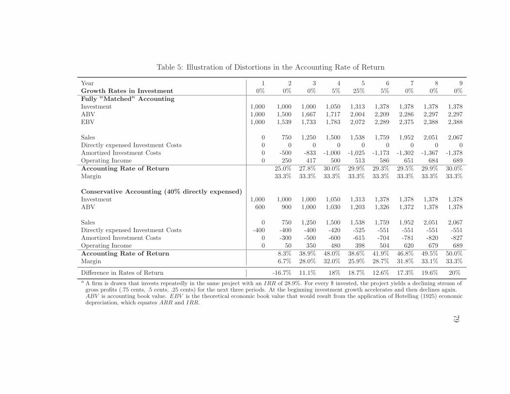
79

Table 5: Illustration of Distortions in the Accounting Rate of Return

Year 1 2 3 4 5 6 7 8 9Growth Rates in Investment 0% 0% 0% 5% 25% 5% 0% 0% 0%Fully ”Matched” AccountingInvestment 1,000 1,000 1,000 1,050 1,313 1,378 1,378 1,378 1,378ABV 1,000 1,500 1,667 1,717 2,004 2,209 2,286 2,297 2,297EBV 1,000 1,539 1,733 1,783 2,072 2,289 2,375 2,388 2,388

Sales 0 750 1,250 1,500 1,538 1,759 1,952 2,051 2,067Directly expensed Investment Costs 0 0 0 0 0 0 0 0 0Amortized Investment Costs 0 -500 -833 -1,000 -1,025 -1,173 -1,302 -1,367 -1,378Operating Income 0 250 417 500 513 586 651 684 689Accounting Rate of Return 25.0% 27.8% 30.0% 29.9% 29.3% 29.5% 29.9% 30.0%Margin 33.3% 33.3% 33.3% 33.3% 33.3% 33.3% 33.3% 33.3%

Conservative Accounting (40% directly expensed)Investment 1,000 1,000 1,000 1,050 1,313 1,378 1,378 1,378 1,378ABV 600 900 1,000 1,030 1,203 1,326 1,372 1,378 1,378

Sales 0 750 1,250 1,500 1,538 1,759 1,952 2,051 2,067Directly expensed Investment Costs -400 -400 -400 -420 -525 -551 -551 -551 -551Amortized Investment Costs 0 -300 -500 -600 -615 -704 -781 -820 -827Operating Income 0 50 350 480 398 504 620 679 689Accounting Rate of Return 8.3% 38.9% 48.0% 38.6% 41.9% 46.8% 49.5% 50.0%Margin 6.7% 28.0% 32.0% 25.9% 28.7% 31.8% 33.1% 33.3%

Difference in Rates of Return -16.7% 11.1% 18% 18.7% 12.6% 17.3% 19.6% 20%a A firm is drawn that invests repeatedly in the same project with an IRR of 28.9%. For every $ invested, the project yields a declining stream ofgross profits (.75 cents, .5 cents, .25 cents) for the next three periods. At the beginning investment growth accelerates and then declines again.ABV is accounting book value. EBV is the theoretical economic book value that would result from the application of Hotelling (1925) economicdepreciation, which equates ARR and IRR.

80

Table 5: Illustration of Distortions in the Accounting Rate of Return (continued)

Year 1 2 3 4 5 6 7 8 9 10 11

DCF CoC= 0.1Outflows 1,000 1,000 1,000 1,050 1,313 1,378 1,378 1,378 1,378 1,378 1,378Inflows 0 750 1,250 1,500 1,538 1,759 1,952 2,051 2,067 2,067 2,067Net CF -1,000 -250 250 450 225 381 574 673 689 689 689Terminal Value at t=11 6,891Discounted Values 227.3 371.9 169.0 260.4 356.5 379.7 353.6 321.5 3,214.5

MV at t=2 5,654

Residual Income Model CoC= 0.1EBV 1,000 1,539 1,733 1,783 2,072 2,289 2,375 2,388 2,388 2,388 2,388Economic Income - 289 444 500 514 598 660 685 689 689 689Economic Rent 0 189 290 327 336 391 432 448 450 450 450Terminal Value at t=11 4,502.9Discounted Values 263.8 270.0 252.6 266.9 268.0 252.8 231.1 210.1 2100.6

EBV at t=2 1,539VER at t=2 4,116

VER+EBV =MV at t=2 5,654a Enterprise-value valuation models for the firm at period t = 2. It is assumed that the market has perfect foresight about thefuture cash streams. The firm depicted is the same firm as in the previous example. The discount rate used is the cost ofcapital at 10%. The residual income model assumes that economic depreciation has been used to amortize the investmentcosts. Then residual income equals economic rent. Economic rent is therefore economic income minus a capital charge of 10%on the economic book value.

81

Table 6: Descriptive Statistics for the Base Sample

Variable Mean StD Min Q1 Median Q3 Max N

Match 0.729 0.414 −1.15 0.680 0.919 0.978 0.999 76342AQ 0.037 0.056 0.000 0.011 0.026 0.048 5.126 49633Acc −.007 0.081 −1.41 −.035 −.003 0.026 1.536 74267TAcc −.010 0.293 −33.8 −.055 −.004 0.040 33.93 60454EarnVol 0.058 0.127 0.000 0.016 0.032 0.067 12.46 76342SalVol 313.5 1483 0.009 10.87 41.31 164.3 68916 76342ChExp −.071 0.384 −27.8 −.186 −.070 0.017 22.35 75881ChRev 0.077 0.343 −14.2 −.021 0.069 0.192 9.713 75882OpCycl 140.7 192.6 0.000 76.22 117.6 171.9 19824 74782PCFO 0.146 0.395 −5.82 −.121 0.149 0.418 8.679 39662PROA 0.376 0.425 −10.2 0.121 0.386 0.621 10.79 75774CapIntan 0.235 0.257 0.000 0.061 0.165 0.328 7.797 34315a Match is the predicted R-squared, PROA the ROA persistence, PCFO CFOpersistence AQ accrual quality, EarnV ol earnings volatility and SalV ol salesvolatility; all computed based on rolling 5 year windows. chExp and ChRev arechanges in expenses (income before ex minus sales) and changes in revenuesdeflated by total assets. Acc is working capital accruals, defined as(△Receiv.+△Invent.−△Payab.−△Tax.−△O.Opr.Liab.). Spec is Compustat’sspecial item variable deflated by total assets.TAcc is total accruals calculated as inRichardson et al. (2005) as WCt +NCOt + FINt − (WCt−1 +NCOt−1 + FINt−1.ARet is abnormal returns calculated by subtracting the return of a size-matchedportfolio. All details to the variable computations can be found in appendix A.

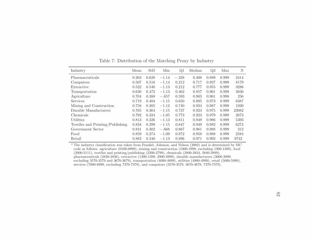
82

Table 7: Distribution of the Matching Proxy by Industry

Industry Mean StD Min Q1 Median Q3 Max N

Pharmaceuticals 0.263 0.628 −1.14 −.328 0.408 0.889 0.999 2414Computers 0.507 0.516 −1.14 0.212 0.717 0.927 0.999 8179Extractive 0.522 0.540 −1.13 0.212 0.777 0.955 0.999 3286Transportation 0.630 0.472 −1.13 0.462 0.857 0.961 0.999 3830Agriculture 0.704 0.388 −.657 0.593 0.903 0.961 0.998 256Services 0.719 0.404 −1.15 0.650 0.895 0.973 0.999 6387Mining and Construction 0.758 0.385 −1.13 0.740 0.934 0.987 0.999 1930Durable Manufacturers 0.765 0.364 −1.15 0.737 0.924 0.975 0.999 23082Chemicals 0.792 0.324 −1.05 0.773 0.923 0.979 0.999 2673Utilities 0.813 0.326 −1.13 0.811 0.949 0.986 0.999 5393Textiles and Printing/Publishing 0.834 0.299 −1.15 0.847 0.949 0.982 0.999 6274Government Sector 0.841 0.302 −.668 0.867 0.961 0.988 0.999 312Food 0.859 0.274 −1.09 0.872 0.958 0.988 0.999 2584Retail 0.882 0.240 −1.13 0.896 0.971 0.992 0.999 9742a The industry classification was taken from Frankel, Johnson, and Nelson (2002) and is determined by SICcode as follows: agriculture (0100-0999), mining and construction (1000-1999, excluding 1300-1399), food(2000-2111), textiles and printing/publishing (2200-2799), chemicals (2800-2824, 2840-2899),pharmaceuticals (2830-2836), extractive (1300-1399, 2900-2999), durable manufacturers (3000-3999,excluding 3570-3579 and 3670-3679), transportation (4000-4899), utilities (4900-4999), retail (5000-5999),services (7000-8999, excluding 7370-7379), and computers (3570-3579, 3670-3679, 7370-7379).

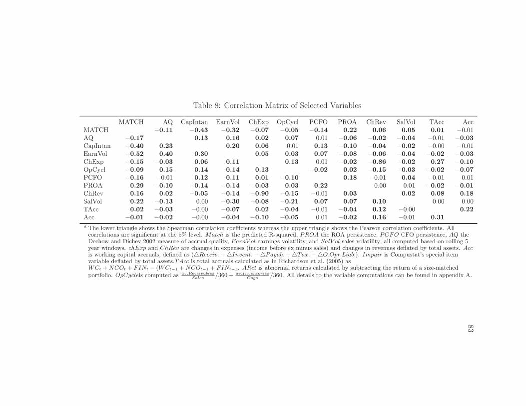
83

Table 8: Correlation Matrix of Selected Variables

MATCH AQ CapIntan EarnVol ChExp OpCycl PCFO PROA ChRev SalVol TAcc AccMATCH −0.11 −0.43 −0.32 −0.07 −0.05 −0.14 0.22 0.06 0.05 0.01 −0.01AQ −0.17 0.13 0.16 0.02 0.07 0.01 −0.06 −0.02 −0.04 −0.01 −0.03CapIntan −0.40 0.23 0.20 0.06 0.01 0.13 −0.10 −0.04 −0.02 −0.00 −0.01EarnVol −0.52 0.40 0.30 0.05 0.03 0.07 −0.08 −0.06 −0.04 −0.02 −0.03ChExp −0.15 −0.03 0.06 0.11 0.13 0.01 −0.02 −0.86 −0.02 0.27 −0.10OpCycl −0.09 0.15 0.14 0.14 0.13 −0.02 0.02 −0.15 −0.03 −0.02 −0.07PCFO −0.16 −0.01 0.12 0.11 0.01 −0.10 0.18 −0.01 0.04 −0.01 0.01PROA 0.29 −0.10 −0.14 −0.14 −0.03 0.03 0.22 0.00 0.01 −0.02 −0.01ChRev 0.16 0.02 −0.05 −0.14 −0.90 −0.15 −0.01 0.03 0.02 0.08 0.18SalVol 0.22 −0.13 0.00 −0.30 −0.08 −0.21 0.07 0.07 0.10 0.00 0.00TAcc 0.02 −0.03 −0.00 −0.07 0.02 −0.04 −0.01 −0.04 0.12 −0.00 0.22Acc −0.01 −0.02 −0.00 −0.04 −0.10 −0.05 0.01 −0.02 0.16 −0.01 0.31a The lower triangle shows the Spearman correlation coefficients whereas the upper triangle shows the Pearson correlation coefficients. Allcorrelations are significant at the 5% level. Match is the predicted R-squared, PROA the ROA persistence, PCFO CFO persistence, AQ theDechow and Dichev 2002 measure of accrual quality, EarnV ol earnings volatility, and SalV ol sales volatility; all computed based on rolling 5year windows. chExp and ChRev are changes in expenses (income before ex minus sales) and changes in revenues deflated by total assets. Accis working capital accruals, defined as (△Receiv.+△Invent.−△Payab.−△Tax.−△O.Opr.Liab.). Impair is Compustat’s special itemvariable deflated by total assets.TAcc is total accruals calculated as in Richardson et al. (2005) asWCt +NCOt + FINt − (WCt−1 +NCOt−1 + FINt−1. ARet is abnormal returns calculated by subtracting the return of a size-matchedportfolio. OpCycleis computed as av.Receivables


Cogs/360. All details to the variable computations can be found in appendix A.

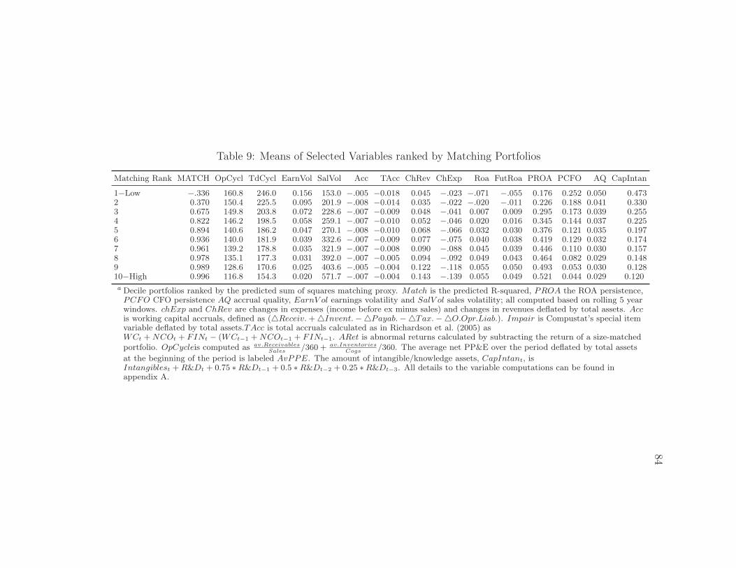
84

Table 9: Means of Selected Variables ranked by Matching Portfolios

Matching Rank MATCH OpCycl TdCycl EarnVol SalVol Acc TAcc ChRev ChExp Roa FutRoa PROA PCFO AQ CapIntan

1−Low −.336 160.8 246.0 0.156 153.0 −.005 −0.018 0.045 −.023 −.071 −.055 0.176 0.252 0.050 0.4732 0.370 150.4 225.5 0.095 201.9 −.008 −0.014 0.035 −.022 −.020 −.011 0.226 0.188 0.041 0.3303 0.675 149.8 203.8 0.072 228.6 −.007 −0.009 0.048 −.041 0.007 0.009 0.295 0.173 0.039 0.2554 0.822 146.2 198.5 0.058 259.1 −.007 −0.010 0.052 −.046 0.020 0.016 0.345 0.144 0.037 0.2255 0.894 140.6 186.2 0.047 270.1 −.008 −0.010 0.068 −.066 0.032 0.030 0.376 0.121 0.035 0.1976 0.936 140.0 181.9 0.039 332.6 −.007 −0.009 0.077 −.075 0.040 0.038 0.419 0.129 0.032 0.1747 0.961 139.2 178.8 0.035 321.9 −.007 −0.008 0.090 −.088 0.045 0.039 0.446 0.110 0.030 0.1578 0.978 135.1 177.3 0.031 392.0 −.007 −0.005 0.094 −.092 0.049 0.043 0.464 0.082 0.029 0.1489 0.989 128.6 170.6 0.025 403.6 −.005 −0.004 0.122 −.118 0.055 0.050 0.493 0.053 0.030 0.12810−High 0.996 116.8 154.3 0.020 571.7 −.007 −0.004 0.143 −.139 0.055 0.049 0.521 0.044 0.029 0.120

a Decile portfolios ranked by the predicted sum of squares matching proxy. Match is the predicted R-squared, PROA the ROA persistence,PCFO CFO persistence AQ accrual quality, EarnV ol earnings volatility and SalV ol sales volatility; all computed based on rolling 5 yearwindows. chExp and ChRev are changes in expenses (income before ex minus sales) and changes in revenues deflated by total assets. Accis working capital accruals, defined as (△Receiv.+△Invent.−△Payab.−△Tax.−△O.Opr.Liab.). Impair is Compustat’s special itemvariable deflated by total assets.TAcc is total accruals calculated as in Richardson et al. (2005) asWCt +NCOt + FINt − (WCt−1 +NCOt−1 + FINt−1. ARet is abnormal returns calculated by subtracting the return of a size-matchedportfolio. OpCycleis computed as av.Receivables


Cogs/360. The average net PP&E over the period deflated by total assets

at the beginning of the period is labeled AvPPE. The amount of intangible/knowledge assets, CapIntant, isIntangiblest +R&Dt + 0.75 ∗R&Dt−1 + 0.5 ∗R&Dt−2 + 0.25 ∗R&Dt−3. All details to the variable computations can be found inappendix A.

85

Table 10: Descriptive Statistics for Selected Conservatism Correction Vari-ables

Variable Mean Std Min Q1 Median Q3 Max N

AT 2368 13636 0.000 55.08 227.4 1077 798E3 76274g 0.611 46.59 −10.4 −.177 0.062 0.354 9626 71279gt 0.110 0.177 −.629 0.026 0.091 0.173 3.183 71181g3 0.118 0.375 −.885 −.069 0.076 0.240 12.50 70489r 0.074 0.045 −.467 0.037 0.100 0.100 1.009 74819T 16.58 6.755 1.000 12.00 16.00 20.00 30.00 71279ABVEBVt 0.652 0.257 0.054 0.451 0.712 0.878 1.000 70861ABVEBV3 0.640 0.259 0.062 0.433 0.675 0.880 0.996 69528ABVEBVV ER 3.822 89.23 0.025 0.421 0.938 1.832 13971 35180VERB 2.272 3.337 0.000 0.614 1.230 2.486 34.25 49233MB 3.196 5.283 0.113 1.019 1.588 3.053 59.82 67190irrt 0.051 15.76 −2256 0.035 0.088 0.151 2686 68150irr3 0.019 9.112 −1373 0.036 0.089 0.151 1055 67028irrV ER −.105 11.73 −891 −.051 0.078 0.161 735.5 35159

a The top and bottom 1% of the key variables ˆCCF , ˆCCF3, ˆCCF

V ER, MtB,

V ERB and g are deleted to control for outliers. AT is the Compustat item totalassets, g is the current periods investment growth rate, g is the historical growthrate, measured as geometric average investment growth rate over the useful life of afirm’s assets. g3 is the geometric average investment growth rate over the past 3years. r is a proxy for the cost of capital, T is the useful life of a firm’s assets.V ERB is the measure of economic-rent-to-book value V ER/ABV . MB is themarket-to-book value. ABV EBV t is the inverse of ˆCCF , which uses the historical

growth rate as input. ABV EBV 3 of ˆCCF3, which uses the average growth rate

over the past 3 years as input and ABV EBV V ER of ˆCCFV ER

. All are measures ofthe ratio of accounting book value to economic book value. The estimationproduces some negative values of ABV EBV FV , which I delete, since this ratiocannot be negative. irrx are measures of the internal rate of return, calculatedusing the inputs above and equation 2.2. irrt is derived using ABV EBV t as input,irr3 is derived using ABV EBV 3 as input, irrV ER is derived using ABV EBV V ER

as input. The detailed variable computation can be found in appendix A.

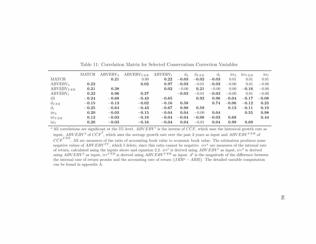
86

Table 11: Correlation Matrix for Selected Conservatism Correction Variables

MATCH ABVEBV3 ABVEBVV ER ABVEBVt d3 dV ER dt irr3 irrV ER irrtMATCH 0.21 0.00 0.22 −0.03 −0.02 −0.03 0.01 0.01 0.01ABVEBV3 0.22 0.02 0.97 −0.03 −0.01 −0.03 −0.00 0.01 −0.00ABVEBVV ER 0.21 0.38 0.02 −0.00 0.21 −0.00 0.00 −0.16 −0.00ABVEBVt 0.22 0.96 0.37 −0.03 −0.01 −0.03 −0.00 0.01 −0.00d3 −0.24 −0.68 −0.43 −0.65 0.92 0.96 −0.04 −0.17 −0.08dV ER −0.15 −0.13 −0.02 −0.16 0.58 0.74 −0.06 −0.12 0.25dt −0.25 −0.64 −0.43 −0.67 0.98 0.59 0.13 −0.11 0.10irr3 0.20 −0.03 −0.15 −0.04 0.04 −0.00 0.04 0.55 0.98irrV ER 0.12 −0.03 −0.16 −0.04 −0.04 −0.08 −0.03 0.68 0.44irrt 0.20 −0.03 −0.16 −0.04 0.04 −0.01 0.04 0.99 0.69

a All correlations are significant at the 5% level. ABV EBV t is the inverse of ˆCCF , which uses the historical growth rate as

input. ABV EBV 3 of ˆCCF3, which uses the average growth rate over the past 3 years as input and ABV EBV V ER of

ˆCCFV ER

. All are measures of the ratio of accounting book value to economic book value. The estimation produces somenegative values of ABV EBV FV , which I delete, since this ratio cannot be negative. irrx are measures of the internal rateof return, calculated using the inputs above and equation 2.2. irrt is derived using ABV EBV t as input, irr3 is derivedusing ABV EBV 3 as input, irrV ER is derived using ABV EBV V ER as input. dt is the magnitude of the difference betweenthe internal rate of return proxies and the accounting rate of return (| ˆIRRx −ARR|). The detailed variable computationcan be found in appendix A.

87

Table 12: EBV/ABV by Matching Rank

Quintile Variable Mean Std Min Q1 Median Q3 Max N

1−Low ABVEBVt 0.549 0.300 0.054 0.262 0.556 0.842 1.000 13416ABVEBV3 0.539 0.299 0.062 0.260 0.526 0.836 0.995 13024

ABVEBVV ER 3.563 151.1 0.025 0.250 0.648 1.313 13971 8620VERB 1.963 3.225 0.000 0.453 0.964 2.029 33.98 8562

MB 4.999 7.950 0.113 1.208 2.089 4.745 59.60 12902

2 ABVEBVt 0.618 0.266 0.054 0.390 0.656 0.863 1.000 14129ABVEBV3 0.606 0.267 0.062 0.375 0.620 0.862 0.996 13844

ABVEBVV ER 2.586 13.84 0.025 0.392 0.866 1.695 459.3 7986VERB 2.128 3.340 0.000 0.543 1.089 2.233 34.20 9956

MB 3.522 5.743 0.113 1.060 1.707 3.364 58.65 13379

3 ABVEBVt 0.657 0.243 0.054 0.463 0.702 0.873 1.000 14439ABVEBV3 0.644 0.247 0.062 0.443 0.666 0.875 0.995 14215

ABVEBVV ER 3.213 19.26 0.026 0.493 1.045 1.990 1017 7116VERB 2.274 3.357 0.000 0.629 1.236 2.471 34.25 10440

MB 2.789 4.125 0.113 0.987 1.524 2.850 59.53 13669

4 ABVEBVt 0.689 0.226 0.057 0.524 0.742 0.881 1.000 14576ABVEBV3 0.676 0.230 0.064 0.500 0.711 0.883 0.995 14382

ABVEBVV ER 4.861 84.71 0.026 0.563 1.149 2.219 6361 6155VERB 2.348 3.181 0.000 0.694 1.343 2.665 33.77 10359

MB 2.413 3.496 0.113 0.939 1.431 2.551 59.53 13674

5−High ABVEBVt 0.740 0.203 0.054 0.601 0.799 0.906 1.000 14301ABVEBVd3 0.725 0.210 0.062 0.575 0.770 0.910 0.996 14063

ABVEBVV ER 5.715 81.21 0.028 0.580 1.180 2.283 3222 5303VERB 2.601 3.527 0.001 0.779 1.498 2.874 33.83 9916

MB 2.358 3.388 0.113 0.956 1.411 2.514 59.82 13566a Ranks are computed each year based on the matching score. ABV EBV t is the inverse of

ˆCCF , which uses the historical growth rate as input. ABV EBV 3 of ˆCCF3, which uses the

average growth rate over the past 3 years as input and ABV EBV V ER of ˆCCFV ER

. Allare measures of the ratio of accounting book value to economic book value. The estimationproduces some negative values of ABV EBV FV , which I delete, since this ratio cannot benegative. V ERB is the measure of economic-rent-to-book value V ER/ABV . MB is themarket-to-book value.

88

Table 13: ARR-IRR by Matching Rank

Quintile Variable Mean Std Min Q1 Median Q3 Max N

1−Low dt 0.950 23.57 0.000 0.013 0.052 0.196 2159 12486d3 1.035 27.81 0.000 0.013 0.053 0.200 2397 12174

dV ER 1.831 43.41 0.000 0.029 0.110 0.372 3192 8614

2 dt 0.309 7.674 0.000 0.009 0.031 0.097 581.6 13517d3 0.284 6.547 0.000 0.009 0.032 0.098 430.9 13285

dV ER 0.951 28.37 0.000 0.021 0.077 0.246 2412 7981

3 dt 0.126 1.469 0.000 0.007 0.022 0.065 103.5 13994d3 0.126 1.330 0.000 0.007 0.023 0.068 92.26 13799

dV ER 0.518 8.405 0.000 0.017 0.061 0.204 656.5 7111

4 dt 0.089 1.334 0.000 0.006 0.019 0.050 116.6 14164d3 0.096 1.742 0.000 0.006 0.020 0.052 175.0 13991

dV ER 0.685 11.37 0.000 0.015 0.054 0.177 735.6 6154

5−High dt 0.087 3.965 0.000 0.004 0.014 0.037 463.4 13989d3 0.087 3.937 0.000 0.004 0.014 0.040 458.0 13779

dV ER 0.674 12.01 0.000 0.013 0.052 0.168 641.5 5299a Ranks are computed each year based on the matching score. dt is the magnitude ofthe difference between the internal rate of return proxies and the accounting rate ofreturn, (| ˆIRRx −ARR|), computed according to equation 2.2 using ABV EBV t, d3

uses ABV EBV 3 and dV ER uses ABV EBV V ER.

89

Table 14: FERC Regressions by Matching Portfolio

Quintile Intercept UE UE1 UE2 UE3 ARet1 ARet2 ARet3 AG EP R2 Obs.

1−Low 0.027 0.006 0.015 0.003 −.002 −.029 −.056 −.018 0.245 −.007 2.56% 7956(0.017) (0.003) (0.004) (0.003) (0.003) (0.028) (0.013) (0.015) (0.041) (0.003)

** *** *** *** **

2 0.033 0.014 0.016 0.003 0.004 −.031 −.019 −.016 0.263 −.008 2.79% 9478(0.011) (0.003) (0.002) (0.002) (0.003) (0.020) (0.014) (0.010) (0.034) (0.002)

*** *** *** *** ***

3 0.016 0.019 0.019 0.007 0.001 0.017 −.047 −.018 0.296 −.006 3.45% 10295(0.015) (0.004) (0.003) (0.002) (0.003) (0.017) (0.016) (0.015) (0.048) (0.001)

*** *** *** *** *** ***

4 0.008 0.021 0.024 0.005 0.001 −.010 −.007 −.010 0.254 −.003 2.83% 10940(0.015) (0.004) (0.004) (0.003) (0.002) (0.022) (0.024) (0.023) (0.046) (0.001)

*** *** ** *** *

5−High 0.024 0.031 0.028 0.005 0.006 −.011 −.015 −.024 0.169 −.003 3.64% 11545(0.014) (0.005) (0.004) (0.002) (0.002) (0.023) (0.022) (0.021) (0.040) (0.002)

* *** *** * ** ***

FTest Y Y Y Y Y Ya Portfolios are formed by sorting observations into four portfolios at the beginning of each year based on their pastMATCH score. The hypothesis that the coefficients for UE are similar across portfolios can be rejected at the 1% levelwith an F-Value of 16.9. The hypothesis that the coefficients for UE1+UE2+UE are similar across portfolios can berejected at the 1% level with an F-Value of 7.73. A Y indicates that High and Low portfolios are significantly different atthe 5% level.

90

C.2 Chapter 3 Tables

Table 15: Descriptive Statistics for Model Variables

Variable N Std Q1 Median Mean Q3

CHEPS 19627 0.105 −.020 0.004 0.005 0.021GM 19627 0.215 −.054 0.003 0.003 0.055SGA 19627 0.205 −.072 −.000 0.009 0.076INV 19627 0.511 −.176 −.017 0.018 0.149CAPX 19627 0.858 −.248 0.065 0.226 0.463LF 19627 0.199 −.027 0.045 0.060 0.124ETR 19627 0.041 −.001 0.000 0.001 0.001DATO 19627 0.038 −.003 −.000 −.001 0.002CRet 19627 0.673 −.267 −.033 0.058 0.227FRet 19627 0.583 −.281 −.052 0.012 0.199FCErr 19627 0.045 −.020 −.003 −.013 0.004FCRev 19627 0.016 −.007 −.001 −.004 0.002Size 19627 1.787 5.245 6.390 6.509 7.638

Table 15: Distribution of INV for each MATCH Quintile (continued)

Matching Portfolio Variable N Std Q1 Median Mean Q3

1−Low INV 3665 0.604 −.240 −.035 0.011 0.173

2 INV 3681 0.556 −.190 −.025 0.020 0.144

3 INV 3678 0.457 −.165 −.011 0.022 0.149

4 INV 3681 0.459 −.145 −.010 0.029 0.144

5−High INV 3672 0.384 −.143 −.010 0.004 0.125a See Table 4 for variable definitions. The sample consists of all firm-years with sufficient

data to compute all listed model variables and don’t have missing observations for all

dependent and explanatory variables. Furthermore, firm-years with either sales less than

$1 million, total assets less than $ 5 million, or a fiscal year shorter than 365 or 366 days

were excluded. To avoid the effect of small denominators, the top and bottom 1% of all

listed variables except for returns and Match were deleted.

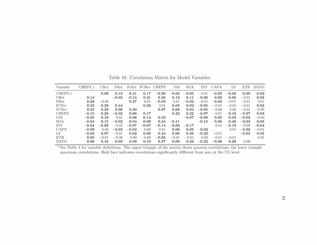
91

Table 16: Correlation Matrix for Model Variables

Variable CHEPS 1 CRet FRet FcErr FCRev CHEPS GM SGA INV CAPX LF ETR DATO

CHEPS 1 0.09 0.19 0.41 0.17 −0.20 −0.05 −0.05 −0.01 −0.05 −0.03 0.09 0.02

CRet 0.14 −0.03 0.14 0.21 0.20 0.12 0.11 −0.06 0.03 0.06 −0.01 0.02

FRet 0.29 −0.00 0.27 0.01 −0.03 0.01 −0.02 −0.01 −0.03 −0.01 0.01 0.01FCErr 0.52 0.26 0.44 0.26 0.01 0.02 0.02 −0.05 −0.01 −0.01 −0.01 0.02

FCRev 0.25 0.39 0.06 0.30 0.07 0.08 0.04 −0.05 −0.00 0.02 −0.01 −0.00CHEPS −0.15 0.28 −0.02 0.06 0.17 0.22 0.22 −0.07 −0.01 0.16 −0.07 0.03

GM −0.05 0.19 0.01 0.06 0.14 0.33 −0.07 −0.06 0.05 0.03 −0.02 −0.00SGA −0.04 0.15 −0.02 0.04 0.09 0.34 −0.11 −0.15 0.06 0.40 −0.03 0.03

INV −0.04 −0.09 −0.02 −0.07 −0.07 −0.14 −0.08 −0.17 0.01 −0.19 −0.00 −0.04

CAPX −0.09 0.00 −0.03 −0.02 0.00 0.01 0.06 0.05 0.02 0.01 −0.02 −0.01LF −0.02 0.07 −0.01 0.02 0.06 0.24 0.06 0.35 −0.22 −0.01 −0.03 0.05

ETR 0.05 −0.01 −0.00 0.00 −0.00 −0.05 −0.01 −0.01 0.00 −0.01 −0.01 0.01DATO 0.06 0.16 0.03 0.09 0.10 0.27 0.09 0.22 −0.22 −0.06 0.28 0.00

a See Table 4 for variable definitions. The upper triangle of the matrix shows pearson correlations, the lower trianglespearman correlations. Bold face indicates correlations significantly different from zero at the 5% level.

92

Table 17: Updating Abarbanell and Bushee (1997) Tests

Yt = α+ β0CHEPSt +∑

7

i=1βiFSi,t + ut

Dependent Intercept CHEPS GM SGA INV CAPX LF ETR DATO R2 Obs.

CHEPS 1 −.003 −.213 −.005 0.005 −.006 −.007 0.002 0.218 0.069 5.09% 19627(0.004) (0.031) (0.009) (0.008) (0.002) (0.001) (0.007) (0.040) (0.025)

*** ** *** *** ***

FCRev −.004 0.007 0.005 −.003 −.001 −.000 −.001 −.000 −.002 1.13% 19627(0.000) (0.002) (0.001) (0.001) (0.000) (0.000) (0.001) (0.005) (0.003)

*** *** *** ** ***

FCErr −.012 −.001 0.005 −.006 −.004 −.001 −.007 −.016 0.025 0.41% 19627(0.002) (0.006) (0.003) (0.003) (0.001) (0.000) (0.003) (0.014) (0.008)

*** * *** * ** ***

CRet 0.048 1.066 0.253 −.236 −.045 0.019 −.034 0.160 0.185 5.23% 19627(0.016) (0.167) (0.042) (0.053) (0.014) (0.011) (0.054) (0.136) (0.120)

*** *** *** *** *** *

FRet 0.017 −.155 0.032 0.052 −.013 −.021 0.007 0.148 0.127 0.21% 19627(0.014) (0.076) (0.031) (0.039) (0.011) (0.005) (0.025) (0.116) (0.158)

* ***a Numbers in parenthesis are two-way cluster-robust standard errors. *** denotes coefficients that aresignificantly different from zero at the 1% level, ** denotes coefficients significant at the 5% level and * atthe 10% level. See Table 4 for variable definitions.

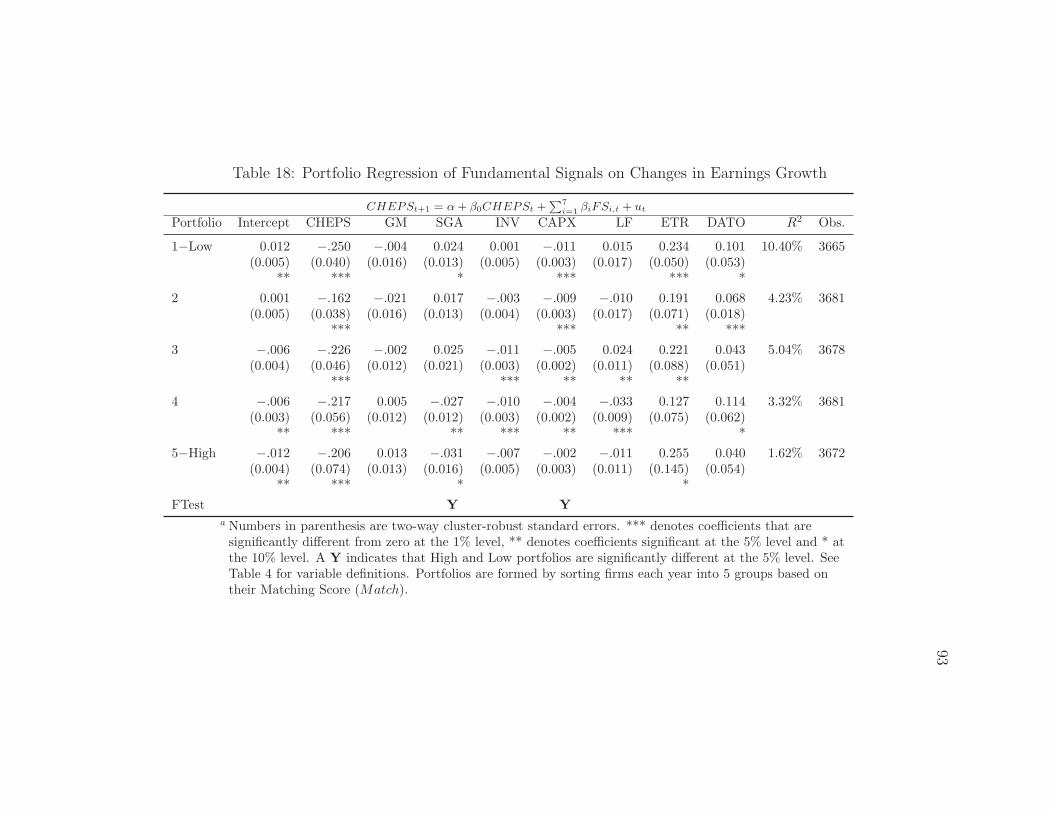
93

Table 18: Portfolio Regression of Fundamental Signals on Changes in Earnings Growth

CHEPSt+1 = α+ β0CHEPSt +∑

7

i=1βiFSi,t + ut

Portfolio Intercept CHEPS GM SGA INV CAPX LF ETR DATO R2 Obs.

1−Low 0.012 −.250 −.004 0.024 0.001 −.011 0.015 0.234 0.101 10.40% 3665(0.005) (0.040) (0.016) (0.013) (0.005) (0.003) (0.017) (0.050) (0.053)

** *** * *** *** *

2 0.001 −.162 −.021 0.017 −.003 −.009 −.010 0.191 0.068 4.23% 3681(0.005) (0.038) (0.016) (0.013) (0.004) (0.003) (0.017) (0.071) (0.018)

*** *** ** ***

3 −.006 −.226 −.002 0.025 −.011 −.005 0.024 0.221 0.043 5.04% 3678(0.004) (0.046) (0.012) (0.021) (0.003) (0.002) (0.011) (0.088) (0.051)

*** *** ** ** **

4 −.006 −.217 0.005 −.027 −.010 −.004 −.033 0.127 0.114 3.32% 3681(0.003) (0.056) (0.012) (0.012) (0.003) (0.002) (0.009) (0.075) (0.062)

** *** ** *** ** *** *

5−High −.012 −.206 0.013 −.031 −.007 −.002 −.011 0.255 0.040 1.62% 3672(0.004) (0.074) (0.013) (0.016) (0.005) (0.003) (0.011) (0.145) (0.054)

** *** * *

FTest Y Ya Numbers in parenthesis are two-way cluster-robust standard errors. *** denotes coefficients that aresignificantly different from zero at the 1% level, ** denotes coefficients significant at the 5% level and * atthe 10% level. A Y indicates that High and Low portfolios are significantly different at the 5% level. SeeTable 4 for variable definitions. Portfolios are formed by sorting firms each year into 5 groups based ontheir Matching Score (Match).

94

Table 19: Portfolio Regression of Fundamental Signals on Forecast Revisions

FCRevt = α+ β0CHEPSt +∑

7

i=1βiFSi,t + ut


1−Low −.006 0.002 0.003 −.002 −.000 0.000 −.001 −.002 −.009 0.25% 3665(0.001) (0.003) (0.002) (0.002) (0.001) (0.000) (0.002) (0.007) (0.008)

*** *

2 −.004 0.004 0.006 −.003 −.002 −.001 0.002 0.014 0.002 1.76% 3681(0.000) (0.003) (0.001) (0.002) (0.001) (0.000) (0.002) (0.015) (0.005)

*** *** ***

3 −.003 0.014 0.004 −.003 −.002 −.001 −.002 −.020 −.007 1.81% 3678(0.001) (0.005) (0.002) (0.002) (0.001) (0.000) (0.002) (0.022) (0.011)

*** ** ** ** **

4 −.003 0.017 0.008 −.006 −.002 −.000 −.003 −.029 0.002 2.82% 3681(0.000) (0.010) (0.003) (0.002) (0.001) (0.000) (0.002) (0.018) (0.009)

*** * *** ** *** *

5−High −.002 0.046 0.006 −.001 −.001 −.000 −.003 0.027 −.010 5.71% 3672(0.000) (0.009) (0.002) (0.002) (0.001) (0.000) (0.001) (0.019) (0.006)

*** *** ** **

FTest Y Ya Numbers in parenthesis are two-way cluster-robust standard errors. *** denotes coefficients that aresignificantly different from zero at the 1% level, ** denotes coefficients significant at the 5% level and *at the 10% level. A Y indicates that High and Low portfolios are significantly different at the 5% level.See Table 4 for variable definitions. Portfolios are formed by sorting firms each year into 5 groups basedon their Matching Score (Match).

95

Table 20: Portfolio Regression of Fundamental Signals on Forecast Errors

FCErrt+1 = α+ β0CHEPSt +∑

7

i=1βiFSi,t + ut


1−Low −.015 −.009 0.002 −.002 −.002 −.000 −.002 −.010 0.032 0.01% 3665(0.002) (0.008) (0.004) (0.005) (0.001) (0.001) (0.006) (0.020) (0.016)

*** *

2 −.014 −.013 −.000 −.007 −.005 −.001 −.007 −.018 0.013 0.34% 3681(0.002) (0.011) (0.004) (0.005) (0.002) (0.001) (0.006) (0.020) (0.010)

*** **

3 −.012 0.012 0.011 −.006 −.007 −.000 −.005 −.018 0.031 0.80% 3678(0.002) (0.019) (0.007) (0.005) (0.003) (0.001) (0.006) (0.027) (0.017)

*** ** *

4 −.010 0.038 0.007 −.013 −.006 −.001 −.020 0.010 0.042 1.51% 3681(0.002) (0.026) (0.009) (0.006) (0.002) (0.001) (0.004) (0.037) (0.027)

*** ** *** ***

5−High −.008 0.102 0.005 −.005 −.003 −.001 −.005 −.020 0.022 2.74% 3672(0.002) (0.033) (0.006) (0.006) (0.001) (0.001) (0.006) (0.045) (0.014)

*** *** *

FTest Ya Numbers in parenthesis are two-way cluster-robust standard errors. *** denotes coefficients that aresignificantly different from zero at the 1% level, ** denotes coefficients significant at the 5% level and *at the 10% level. A Y indicates that High and Low portfolios are significantly different at the 5% level.See Table 4 for variable definitions. Portfolios are formed by sorting firms each year into 5 groups basedon their Matching Score (Match).

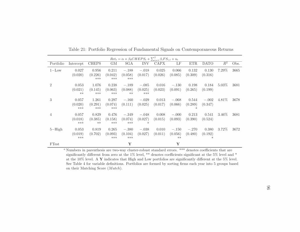
96

Table 21: Portfolio Regression of Fundamental Signals on Contemporaneous Returns

Rett = α+ β0CHEPSt +∑

7

i=1βiFSi,t + ut


1−Low 0.027 0.956 0.211 −.188 −.018 0.025 0.066 0.132 0.130 7.29% 3665(0.020) (0.226) (0.042) (0.058) (0.017) (0.026) (0.085) (0.309) (0.316)

*** *** ***

2 0.053 1.076 0.238 −.189 −.085 0.016 −.130 0.198 0.184 5.03% 3681(0.021) (0.145) (0.063) (0.088) (0.025) (0.023) (0.091) (0.265) (0.199)

** *** *** ** ***

3 0.057 1.261 0.297 −.160 −.029 0.013 −.068 0.544 −.002 4.81% 3678(0.020) (0.291) (0.074) (0.111) (0.025) (0.017) (0.066) (0.289) (0.347)

*** *** *** *

4 0.057 0.829 0.476 −.349 −.048 0.008 −.000 0.213 0.541 3.46% 3681(0.018) (0.385) (0.158) (0.074) (0.027) (0.015) (0.093) (0.390) (0.524)

*** ** *** *** *

5−High 0.053 0.819 0.265 −.380 −.038 0.010 −.150 −.270 0.380 3.72% 3672(0.019) (0.702) (0.093) (0.104) (0.027) (0.011) (0.056) (0.480) (0.192)

*** *** *** ** *

FTest Y Ya Numbers in parenthesis are two-way cluster-robust standard errors. *** denotes coefficients that aresignificantly different from zero at the 1% level, ** denotes coefficients significant at the 5% level and *at the 10% level. A Y indicates that High and Low portfolios are significantly different at the 5% level.See Table 4 for variable definitions. Portfolios are formed by sorting firms each year into 5 groups basedon their Matching Score (Match).

97

Table 22: Portfolio Regression of Fundamental Signals on Future Returns

Rett+1 = α+ β0CHEPSt +∑

7

i=1βiFSi,t + ut


1−Low 0.024 −.125 −.001 0.010 0.012 −.031 0.000 0.246 −.075 0.20% 3665(0.018) (0.110) (0.043) (0.054) (0.020) (0.010) (0.064) (0.189) (0.424)

***

2 0.018 −.221 0.037 0.094 −.043 −.035 0.010 0.029 0.052 0.45% 3681(0.015) (0.087) (0.060) (0.094) (0.026) (0.014) (0.063) (0.189) (0.174)

** **

3 0.017 −.130 0.020 0.087 −.035 −.006 0.002 0.102 0.345 0.08% 3678(0.015) (0.115) (0.054) (0.092) (0.019) (0.009) (0.066) (0.158) (0.422)

*

4 0.018 −.266 0.099 −.106 0.012 −.006 −.007 0.670 0.329 0.04% 3681(0.018) (0.254) (0.079) (0.102) (0.031) (0.018) (0.063) (0.330) (0.243)

*

5−High 0.006 −.184 0.028 0.049 −.061 −.006 0.007 0.125 0.229 0.19% 3672(0.015) (0.185) (0.065) (0.056) (0.019) (0.012) (0.036) (0.261) (0.180)

***

FTest Ya Numbers in parenthesis are two-way cluster-robust standard errors. *** denotes coefficients that aresignificantly different from zero at the 1% level, ** denotes coefficients significant at the 5% level and *at the 10% level. A Y indicates that High and Low portfolios are significantly different at the 5% level.See Table 4 for variable definitions. Portfolios are formed by sorting firms each year into 5 groups basedon their Matching Score (Match).

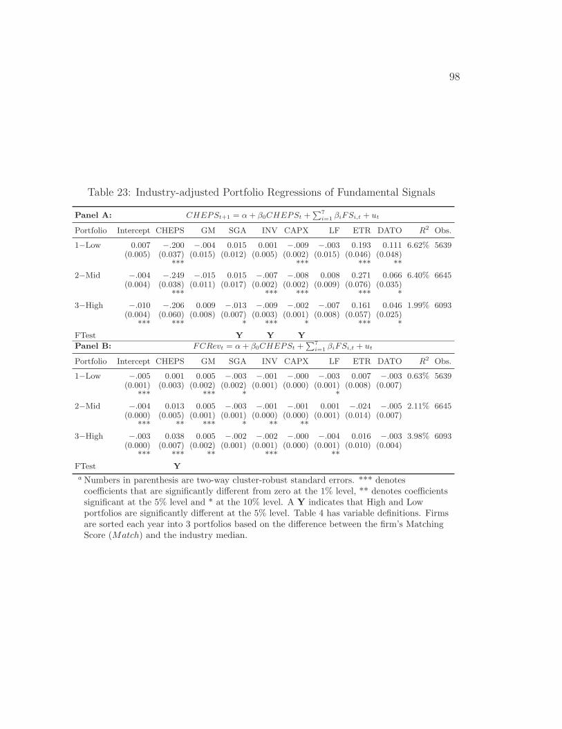
98

Table 23: Industry-adjusted Portfolio Regressions of Fundamental Signals

Panel A: CHEPSt+1 = α+ β0CHEPSt +∑

7

i=1βiFSi,t + ut


1−Low 0.007 −.200 −.004 0.015 0.001 −.009 −.003 0.193 0.111 6.62% 5639(0.005) (0.037) (0.015) (0.012) (0.005) (0.002) (0.015) (0.046) (0.048)

*** *** *** **

2−Mid −.004 −.249 −.015 0.015 −.007 −.008 0.008 0.271 0.066 6.40% 6645(0.004) (0.038) (0.011) (0.017) (0.002) (0.002) (0.009) (0.076) (0.035)

*** *** *** *** *

3−High −.010 −.206 0.009 −.013 −.009 −.002 −.007 0.161 0.046 1.99% 6093(0.004) (0.060) (0.008) (0.007) (0.003) (0.001) (0.008) (0.057) (0.025)

*** *** * *** * *** *

FTest Y Y Y

Panel B: FCRevt = α+ β0CHEPSt +∑

7

i=1βiFSi,t + ut


1−Low −.005 0.001 0.005 −.003 −.001 −.000 −.003 0.007 −.003 0.63% 5639(0.001) (0.003) (0.002) (0.002) (0.001) (0.000) (0.001) (0.008) (0.007)

*** *** * *

2−Mid −.004 0.013 0.005 −.003 −.001 −.001 0.001 −.024 −.005 2.11% 6645(0.000) (0.005) (0.001) (0.001) (0.000) (0.000) (0.001) (0.014) (0.007)

*** ** *** * ** **

3−High −.003 0.038 0.005 −.002 −.002 −.000 −.004 0.016 −.003 3.98% 6093(0.000) (0.007) (0.002) (0.001) (0.001) (0.000) (0.001) (0.010) (0.004)

*** *** ** *** **

FTest Y

a Numbers in parenthesis are two-way cluster-robust standard errors. *** denotescoefficients that are significantly different from zero at the 1% level, ** denotes coefficientssignificant at the 5% level and * at the 10% level. A Y indicates that High and Lowportfolios are significantly different at the 5% level. Table 4 has variable definitions. Firmsare sorted each year into 3 portfolios based on the difference between the firm’s MatchingScore (Match) and the industry median.

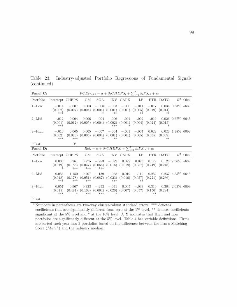
99

Table 23: Industry-adjusted Portfolio Regressions of Fundamental Signals(continued)

Panel C: FCErrt+1 = α+ β0CHEPSt +∑

7

i=1βiFSi,t + ut


1−Low −.014 −.007 0.003 −.008 −.003 −.000 −.014 −.017 0.034 0.33% 5639(0.002) (0.007) (0.004) (0.004) (0.001) (0.001) (0.005) (0.019) (0.014)

*** * ** ** **

2−Mid −.012 0.004 0.006 −.004 −.006 −.001 −.002 −.019 0.026 0.67% 6645(0.001) (0.012) (0.005) (0.004) (0.002) (0.001) (0.004) (0.024) (0.015)

*** *** * *

3−High −.010 0.065 0.005 −.007 −.004 −.001 −.007 0.023 0.023 1.38% 6093(0.002) (0.023) (0.005) (0.004) (0.001) (0.001) (0.005) (0.035) (0.009)

*** *** * ** **

FTest Y

Panel D: Rett = α+ β0CHEPSt +∑

7

i=1βiFSi,t + ut


1−Low 0.033 0.961 0.275 −.283 −.022 0.022 0.023 0.179 0.123 7.36% 5639(0.019) (0.185) (0.047) (0.065) (0.016) (0.018) (0.057) (0.249) (0.246)

* *** *** ***

2−Mid 0.056 1.150 0.207 −.139 −.068 0.019 −.119 0.252 0.237 4.55% 6645(0.018) (0.178) (0.051) (0.087) (0.023) (0.016) (0.057) (0.221) (0.236)

*** *** *** *** **

3−High 0.057 0.967 0.323 −.252 −.041 0.005 −.033 0.310 0.364 2.63% 6093(0.015) (0.491) (0.108) (0.064) (0.020) (0.007) (0.057) (0.150) (0.284)

*** * *** *** * **

FTest


100

Table 23: Industry-adjusted Portfolio Regressions of Fundamental Signals(continued)

Panel E: Rett+1 = α+ β0CHEPSt +∑

7

i=1βiFSi,t + ut


1−Low 0.017 −.118 −.005 0.031 0.001 −.031 0.013 0.206 0.053 0.21% 5639(0.014) (0.089) (0.038) (0.047) (0.020) (0.010) (0.061) (0.181) (0.295)

***

2−Mid 0.017 −.214 0.065 0.052 −.040 −.021 0.001 0.130 0.144 0.36% 6645(0.015) (0.099) (0.049) (0.071) (0.019) (0.005) (0.030) (0.136) (0.231)

** ** ***

3−High 0.015 −.295 0.022 −.004 −.016 −.002 −.000 0.267 0.249 0.00% 6093(0.013) (0.216) (0.059) (0.059) (0.027) (0.007) (0.031) (0.218) (0.108)

**

FTest Y


101

C.3 Chapter 4 Figures and Tables

(a) Earnings Growth (b) Sales Growth

(c) Investment Intensity (d) Forecast Error vs EG

Figure 3: Investment Growth vs. Selected Variables forHighest IG Quintile inside Highest Conservatism QuintilePlots the main variables of interest for the top quintile of firm-years with the highest investment growth

inside the highest average past conservatism quintile. IG is investment growth. EG1 is earnings growth

EGt. gSG1 is sales growth SGt. RDInt is R&D to Sales and Err is the consensus forecast error Err.

102

(a) △ II vs EG

(b) IG vs EG

Figure 4: △ Investment Intensity vs Investment Growth forHighest △II Quintile inside Highest Conservatism QuintilePlots the main variables of interest for the top quintile of firm-years with the highest change investment

intensity inside the highest average past conservatism quintile. IG is investment growth. EG1 is earnings

growth EGt. dIIt is the change in investment intensity.

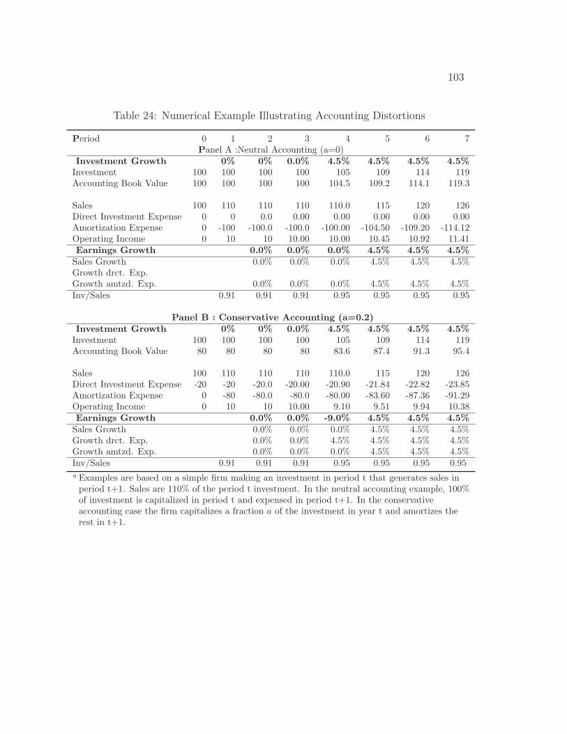
103

Table 24: Numerical Example Illustrating Accounting Distortions

Period 0 1 2 3 4 5 6 7Panel A :Neutral Accounting (a=0)

Investment Growth 0% 0% 0.0% 4.5% 4.5% 4.5% 4.5%Investment 100 100 100 100 105 109 114 119Accounting Book Value 100 100 100 100 104.5 109.2 114.1 119.3

Sales 100 110 110 110 110.0 115 120 126Direct Investment Expense 0 0 0.0 0.00 0.00 0.00 0.00 0.00Amortization Expense 0 -100 -100.0 -100.0 -100.00 -104.50 -109.20 -114.12Operating Income 0 10 10 10.00 10.00 10.45 10.92 11.41Earnings Growth 0.0% 0.0% 0.0% 4.5% 4.5% 4.5%Sales Growth 0.0% 0.0% 0.0% 4.5% 4.5% 4.5%Growth drct. Exp.Growth amtzd. Exp. 0.0% 0.0% 0.0% 4.5% 4.5% 4.5%Inv/Sales 0.91 0.91 0.91 0.95 0.95 0.95 0.95

Panel B : Conservative Accounting (a=0.2)Investment Growth 0% 0% 0.0% 4.5% 4.5% 4.5% 4.5%Investment 100 100 100 100 105 109 114 119Accounting Book Value 80 80 80 80 83.6 87.4 91.3 95.4

Sales 100 110 110 110 110.0 115 120 126Direct Investment Expense -20 -20 -20.0 -20.00 -20.90 -21.84 -22.82 -23.85Amortization Expense 0 -80 -80.0 -80.0 -80.00 -83.60 -87.36 -91.29Operating Income 0 10 10 10.00 9.10 9.51 9.94 10.38Earnings Growth 0.0% 0.0% -9.0% 4.5% 4.5% 4.5%Sales Growth 0.0% 0.0% 0.0% 4.5% 4.5% 4.5%Growth drct. Exp. 0.0% 0.0% 4.5% 4.5% 4.5% 4.5%Growth amtzd. Exp. 0.0% 0.0% 0.0% 4.5% 4.5% 4.5%Inv/Sales 0.91 0.91 0.91 0.95 0.95 0.95 0.95a Examples are based on a simple firm making an investment in period t that generates sales inperiod t+1. Sales are 110% of the period t investment. In the neutral accounting example, 100%of investment is capitalized in period t and expensed in period t+1. In the conservativeaccounting case the firm capitalizes a fraction a of the investment in year t and amortizes therest in t+1.

104

Table 25: Descriptive Statistics for Model Variables

Variable N Std Q1 Median Mean Q3

dEG 18963 1.990 −.549 −.056 −.075 0.360Err 17591 0.758 −.352 −.029 −.277 0.103FCRev 17692 1.058 −.423 −.055 −.208 0.178EG 18963 1.018 −.192 0.125 0.132 0.431II 19755 0.765 0.073 0.131 0.271 0.231dII 18955 0.312 −.198 −.039 −.009 0.138IG 19755 0.580 −.105 0.069 0.146 0.274SG 18951 0.223 −.004 0.088 0.118 0.204GM 18963 0.225 0.283 0.411 0.426 0.575ACons 19755 0.264 0.335 0.574 0.545 0.770WCacc 19465 0.094 −.023 0.006 0.009 0.040T 19732 6.772 9.000 13.00 14.24 18.00RoE 18962 0.216 0.029 0.122 0.093 0.202EVol 18963 0.024 0.000 0.002 0.011 0.009a dEG is the change in earnings growth EGt − EGt−1 with

(Et − Et−1)/|Et−1|. Et is IBES actual unadjusted eps times shares

outstanding at the fiscal year end. II is investment intensity,

Inv/Sale, and IGt is investment growth computed as

(Invt/Invt−1 − 1) where invt is the sum of the current year’s R&D

expenses, advertising and capital expenditures

(XRDt +XADt + CAPXVt). Const is the measure for

unconditional conservatism and is computed as

(XRDt +XADt)/(XRDt +XADt + CAPXVt). ACons is the

geometric moving average over the past 3 years of Cons. dIIt−1 is

lagged change in investment intensity. See appendix A for the

remaining variable definitions.

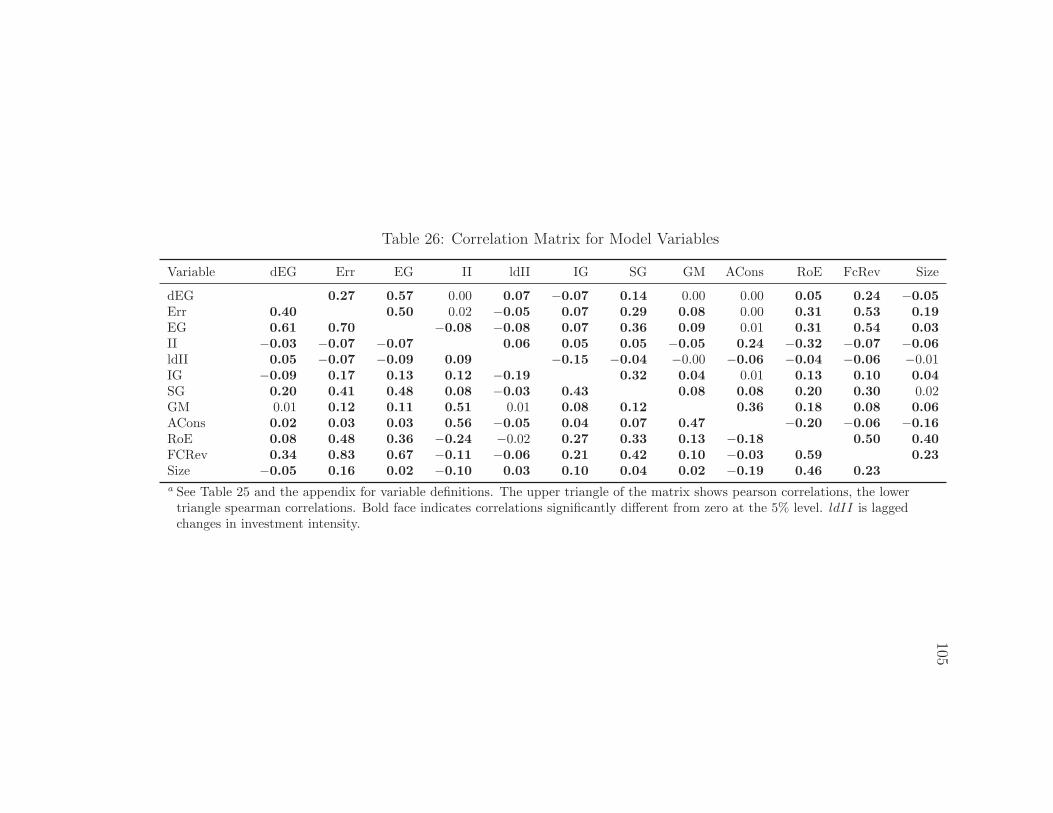
105

Table 26: Correlation Matrix for Model Variables

Variable dEG Err EG II ldII IG SG GM ACons RoE FcRev Size

dEG 0.27 0.57 0.00 0.07 −0.07 0.14 0.00 0.00 0.05 0.24 −0.05Err 0.40 0.50 0.02 −0.05 0.07 0.29 0.08 0.00 0.31 0.53 0.19EG 0.61 0.70 −0.08 −0.08 0.07 0.36 0.09 0.01 0.31 0.54 0.03II −0.03 −0.07 −0.07 0.06 0.05 0.05 −0.05 0.24 −0.32 −0.07 −0.06ldII 0.05 −0.07 −0.09 0.09 −0.15 −0.04 −0.00 −0.06 −0.04 −0.06 −0.01IG −0.09 0.17 0.13 0.12 −0.19 0.32 0.04 0.01 0.13 0.10 0.04SG 0.20 0.41 0.48 0.08 −0.03 0.43 0.08 0.08 0.20 0.30 0.02GM 0.01 0.12 0.11 0.51 0.01 0.08 0.12 0.36 0.18 0.08 0.06ACons 0.02 0.03 0.03 0.56 −0.05 0.04 0.07 0.47 −0.20 −0.06 −0.16RoE 0.08 0.48 0.36 −0.24 −0.02 0.27 0.33 0.13 −0.18 0.50 0.40FCRev 0.34 0.83 0.67 −0.11 −0.06 0.21 0.42 0.10 −0.03 0.59 0.23Size −0.05 0.16 0.02 −0.10 0.03 0.10 0.04 0.02 −0.19 0.46 0.23a See Table 25 and the appendix for variable definitions. The upper triangle of the matrix shows pearson correlations, the lowertriangle spearman correlations. Bold face indicates correlations significantly different from zero at the 5% level. ldII is laggedchanges in investment intensity.

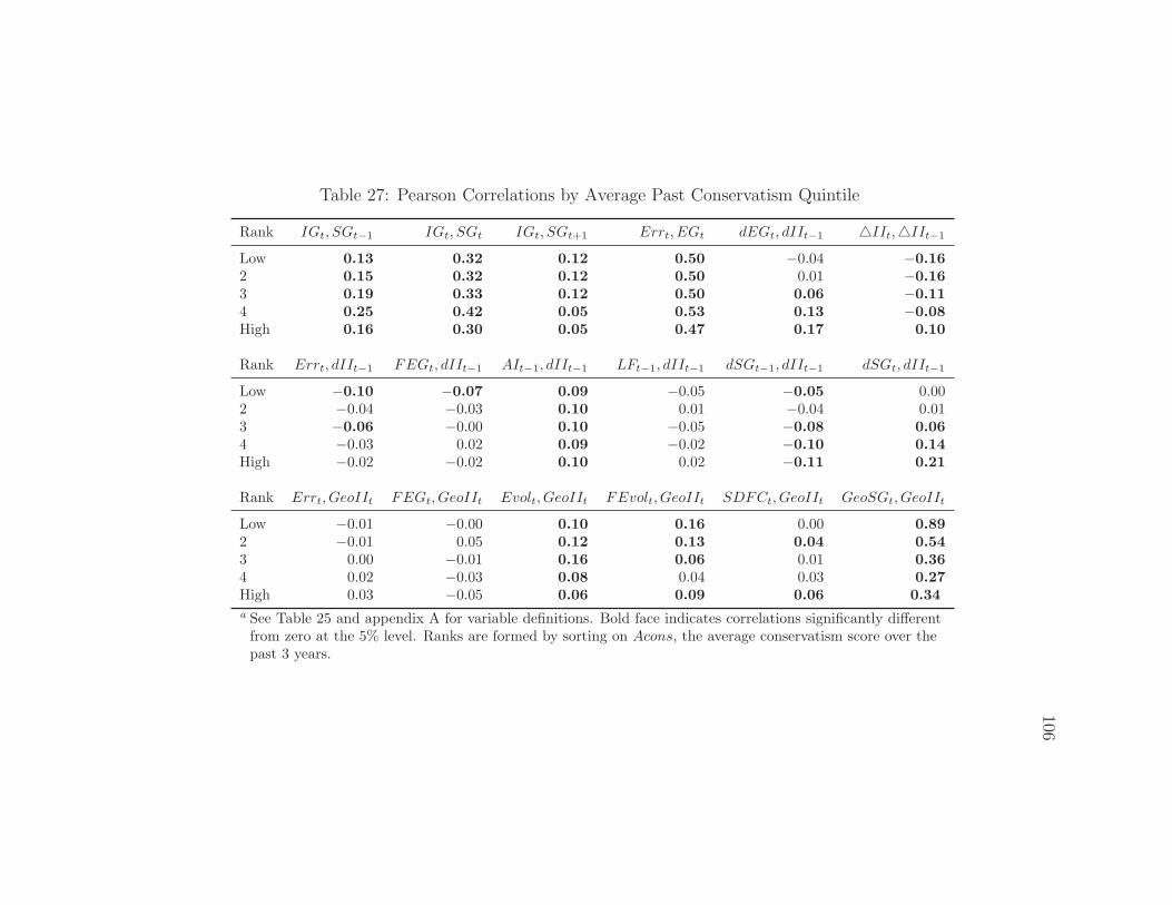
106

Table 27: Pearson Correlations by Average Past Conservatism Quintile

Rank IGt, SGt−1 IGt, SGt IGt, SGt+1 Errt, EGt dEGt, dIIt−1 △IIt,△IIt−1

Low 0.13 0.32 0.12 0.50 −0.04 −0.162 0.15 0.32 0.12 0.50 0.01 −0.163 0.19 0.33 0.12 0.50 0.06 −0.114 0.25 0.42 0.05 0.53 0.13 −0.08High 0.16 0.30 0.05 0.47 0.17 0.10

Rank Errt, dIIt−1 FEGt, dIIt−1 AIt−1, dIIt−1 LFt−1, dIIt−1 dSGt−1, dIIt−1 dSGt, dIIt−1

Low −0.10 −0.07 0.09 −0.05 −0.05 0.002 −0.04 −0.03 0.10 0.01 −0.04 0.013 −0.06 −0.00 0.10 −0.05 −0.08 0.064 −0.03 0.02 0.09 −0.02 −0.10 0.14High −0.02 −0.02 0.10 0.02 −0.11 0.21

Rank Errt, GeoIIt FEGt, GeoIIt Evolt, GeoIIt FEvolt, GeoIIt SDFCt, GeoIIt GeoSGt, GeoIIt

Low −0.01 −0.00 0.10 0.16 0.00 0.892 −0.01 0.05 0.12 0.13 0.04 0.543 0.00 −0.01 0.16 0.06 0.01 0.364 0.02 −0.03 0.08 0.04 0.03 0.27High 0.03 −0.05 0.06 0.09 0.06 0.34a See Table 25 and appendix A for variable definitions. Bold face indicates correlations significantly differentfrom zero at the 5% level. Ranks are formed by sorting on Acons, the average conservatism score over thepast 3 years.

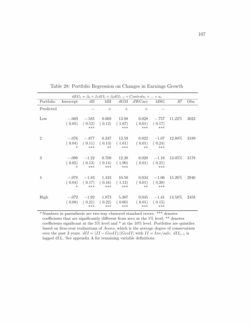
107

Table 28: Portfolio Regression on Changes in Earnings Growth

dEGt = β0 + β1dIIt + β2dIIt−1 + Controlst + ...+ ut

Portfolio Intercept dII ldII dGM dWCacc ldSG R2 Obs.

Predicted − + + + −

Low −.069 −.585 0.069 13.98 0.028 −.757 11.22% 3022( 0.05) ( 0.12) ( 0.12) ( 1.67) ( 0.01) ( 0.17)

*** *** *** ***

2 −.076 −.877 0.337 13.59 0.022 −1.07 12.80% 3189( 0.04) ( 0.11) ( 0.13) ( 1.61) ( 0.01) ( 0.24)

* *** ** *** ** ***

3 −.098 −1.22 0.709 12.20 0.020 −1.16 13.05% 3178( 0.05) ( 0.13) ( 0.14) ( 1.90) ( 0.01) ( 0.21)

* *** *** *** ***

4 −.078 −1.83 1.433 10.50 0.034 −1.06 15.26% 2946( 0.04) ( 0.17) ( 0.16) ( 1.12) ( 0.01) ( 0.20)

* *** *** *** ** ***

High −.072 −1.92 1.873 5.387 0.045 −1.41 14.58% 2458( 0.08) ( 0.21) ( 0.22) ( 0.60) ( 0.01) ( 0.15)

*** *** *** *** ***a Numbers in parenthesis are two-way clustered standard errors. *** denotescoefficients that are significantly different from zero at the 1% level, ** denotescoefficients significant at the 5% level and * at the 10% level. Portfolios are quintilesbased on firm-year realizations of Acons, which is the average degree of conservatismover the past 3 years. dII = (II −GeoII)/|GeoII| with II = Inv/sale. dIIt−1 islagged dIIt. See appendix A for remaining variable definitions.

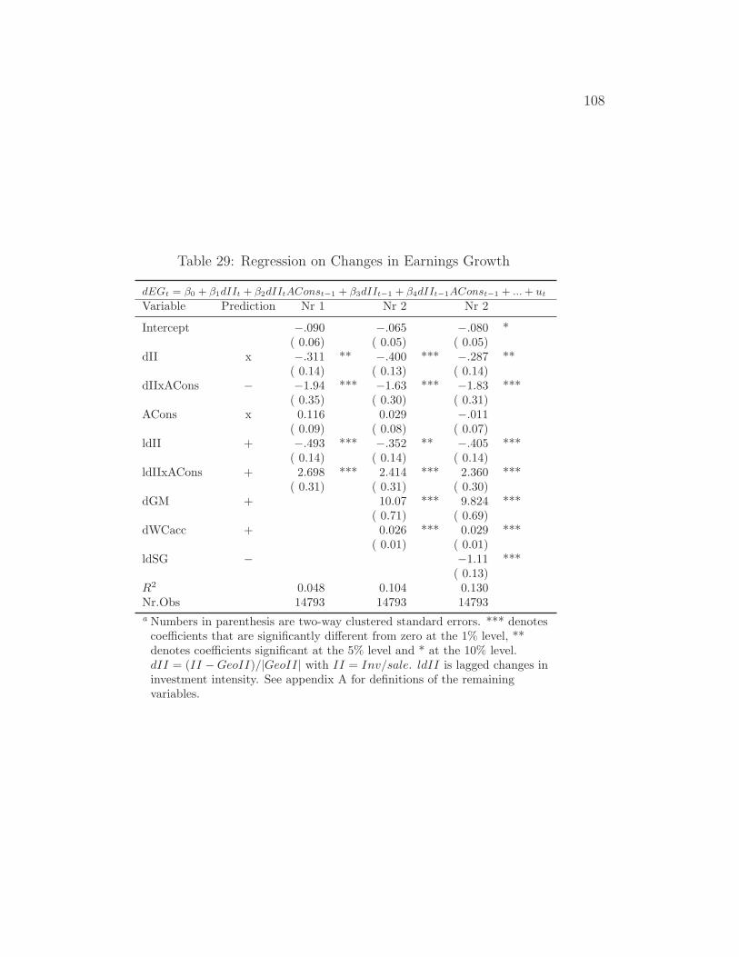
108

Table 29: Regression on Changes in Earnings Growth

dEGt = β0 + β1dIIt + β2dIItAConst−1 + β3dIIt−1 + β4dIIt−1AConst−1 + ...+ ut

Variable Prediction Nr 1 Nr 2 Nr 2

Intercept −.090 −.065 −.080 *( 0.06) ( 0.05) ( 0.05)

dII x −.311 ** −.400 *** −.287 **( 0.14) ( 0.13) ( 0.14)

dIIxACons − −1.94 *** −1.63 *** −1.83 ***( 0.35) ( 0.30) ( 0.31)

ACons x 0.116 0.029 −.011( 0.09) ( 0.08) ( 0.07)

ldII + −.493 *** −.352 ** −.405 ***( 0.14) ( 0.14) ( 0.14)

ldIIxACons + 2.698 *** 2.414 *** 2.360 ***( 0.31) ( 0.31) ( 0.30)

dGM + 10.07 *** 9.824 ***( 0.71) ( 0.69)

dWCacc + 0.026 *** 0.029 ***( 0.01) ( 0.01)

ldSG − −1.11 ***( 0.13)

R2 0.048 0.104 0.130Nr.Obs 14793 14793 14793a Numbers in parenthesis are two-way clustered standard errors. *** denotescoefficients that are significantly different from zero at the 1% level, **denotes coefficients significant at the 5% level and * at the 10% level.dII = (II −GeoII)/|GeoII| with II = Inv/sale. ldII is lagged changes ininvestment intensity. See appendix A for definitions of the remainingvariables.

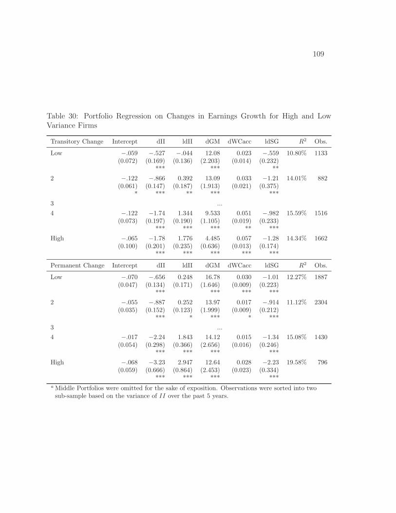
109

Table 30: Portfolio Regression on Changes in Earnings Growth for High and LowVariance Firms

Transitory Change Intercept dII ldII dGM dWCacc ldSG R2 Obs.

Low −.059 −.527 −.044 12.08 0.023 −.559 10.80% 1133(0.072) (0.169) (0.136) (2.203) (0.014) (0.232)

*** *** **

2 −.122 −.866 0.392 13.09 0.033 −1.21 14.01% 882(0.061) (0.147) (0.187) (1.913) (0.021) (0.375)

* *** ** *** ***

3 ...

4 −.122 −1.74 1.344 9.533 0.051 −.982 15.59% 1516(0.073) (0.197) (0.190) (1.105) (0.019) (0.233)

*** *** *** ** ***

High −.065 −1.78 1.776 4.485 0.057 −1.28 14.34% 1662(0.100) (0.201) (0.235) (0.636) (0.013) (0.174)

*** *** *** *** ***

Permanent Change Intercept dII ldII dGM dWCacc ldSG R2 Obs.

Low −.070 −.656 0.248 16.78 0.030 −1.01 12.27% 1887(0.047) (0.134) (0.171) (1.646) (0.009) (0.223)

*** *** *** ***

2 −.055 −.887 0.252 13.97 0.017 −.914 11.12% 2304(0.035) (0.152) (0.123) (1.999) (0.009) (0.212)

*** * *** * ***

3 ...

4 −.017 −2.24 1.843 14.12 0.015 −1.34 15.08% 1430(0.054) (0.298) (0.366) (2.656) (0.016) (0.246)

*** *** *** ***

High −.068 −3.23 2.947 12.64 0.028 −2.23 19.58% 796(0.059) (0.666) (0.864) (2.453) (0.023) (0.334)

*** *** *** ***a Middle Portfolios were omitted for the sake of exposition. Observations were sorted into twosub-sample based on the variance of II over the past 5 years.

110

Table 31: Portfolio Regression on Analyst Forecast Errors

Errt = β0 + β1dIIt−1 + Controlst−1 + ...+ ut

Portfolio Intercept ldII SDFc AOL EVol Size lE ldSG ldGM lIG AI LF Numest R2 Obs.

Low −.834 −.136 −.531 0.001 −5.36 0.070 2.795 0.076 0.740 0.014 −.256 −.404 −.001 17.88% 2019( 0.11) ( 0.06) ( 0.15) ( 0.00) ( 4.68) ( 0.01) ( 0.31) ( 0.08) ( 0.67) ( 0.07) ( 0.08) ( 0.13) ( 0.00)

*** ** *** *** *** *** ***

2 −.708 0.010 −.350 0.001 −7.92 0.084 2.482 0.041 0.664 −.137 −.038 0.010 −.014 15.73% 2162( 0.15) ( 0.08) ( 0.19) ( 0.00) ( 3.51) ( 0.02) ( 0.28) ( 0.09) ( 0.48) ( 0.06) ( 0.08) ( 0.18) ( 0.00)

*** * ** *** *** ** ***

3 −.816 −.091 −.648 0.002 −3.67 0.079 1.987 0.048 −.315 −.039 −.179 −.127 −.005 15.02% 2139( 0.17) ( 0.09) ( 0.21) ( 0.00) ( 3.20) ( 0.01) ( 0.32) ( 0.10) ( 0.32) ( 0.09) ( 0.06) ( 0.12) ( 0.00)

*** *** ** *** *** ***

4 −.513 −.024 −.968 0.002 0.148 0.048 1.962 −.031 0.364 −.173 −.066 −.155 0.005 15.11% 1668( 0.15) ( 0.10) ( 0.27) ( 0.00) ( 1.47) ( 0.01) ( 0.22) ( 0.08) ( 0.29) ( 0.13) ( 0.05) ( 0.15) ( 0.00)

*** *** ** *** *** **

High −.575 0.183 −.509 0.001 −1.11 0.063 0.869 −.104 −.002 −.113 −.179 −.023 0.006 8.11% 1033( 0.20) ( 0.09) ( 0.33) ( 0.00) ( 0.88) ( 0.02) ( 0.16) ( 0.04) ( 0.05) ( 0.10) ( 0.07) ( 0.13) ( 0.00)

*** ** *** *** ** **

a Numbers in parenthesis are two-way clustered standard errors. *** denotes coefficients that are significantly differentfrom zero at the 1% level, ** denotes coefficients significant at the 5% level and * at the 10% level. Portfolios arequintiles based on firm-year realizations of Acons, which is the average degree of conservatism over the past 3 years.dII = (II −GeoII)/|GeoII| with II = Inv/sale. ldII is lagged changes in investment intensity. See appendix A forremaining variable definitions.

111

Table 32: Regression on Analyst Forecast Errors

Errt = β0 + β1AConst−1 + β2dIIt−1 + β3dIIt−1AConst−1 + ...+ ut

Variable Prediction Nr 1 Nr 2 Nr 3 Nr 4

Intercept −.224 *** −.142 *** −.810 *** −.716 ***( 0.03) ( 0.02) ( 0.06) ( 0.12)

ACons + −.076 −.117 ** 0.009 0.048( 0.05) ( 0.05) ( 0.04) ( 0.04)

ldII + −.272 *** −.266 *** −.253 *** −.152 **( 0.05) ( 0.05) ( 0.05) ( 0.07)

ldIIxACons + 0.263 ** 0.261 ** 0.306 *** 0.213 **( 0.11) ( 0.11) ( 0.10) ( 0.10)

SDFc − −.657 *** −.819 *** −.595 ***( 0.13) ( 0.11) ( 0.09)

AOL − 0.001 ** 0.001 ***( 0.00) ( 0.00)

EVol − −6.67 *** −1.93( 1.72) ( 1.43)

Size + 0.090 *** 0.070 ***( 0.01) ( 0.01)

lE + 1.799 ***( 0.13)

ldSG + 0.014( 0.04)

ldGM + −.012( 0.08)

lIG x −.075( 0.06)

AI − −.148 ***( 0.03)

LF − −.178 *( 0.10)

Numest + −.002( 0.00)

R2 0.004 0.014 0.079 0.132Nr.Obs 9021 9021 9021 9021

a Numbers in parenthesis are two-way clustered standard errors. ***denotes coefficients significantly different from zero at the 1%level, ** denotes coefficients significant at the 5% level and * atthe 10% level. See appendix A for variable definitions.

112

Table 33: Portfolio Regression on Analyst Forecast Revisions

FCRevt = β0 + β1dIIt−1 + Controlst−1 + ...+ ut

Portfolio Intercept ldII SDFc EVol Size lE ldSG ldGM lIG AI LF Numest R2 Obs.

Low −.944 −.113 −.691 −4.06 0.096 3.419 0.133 2.597 0.066 −.136 −.149 −.002 19.95% 2070( 0.12) ( 0.09) ( 0.21) ( 3.78) ( 0.02) ( 0.59) ( 0.12) ( 0.89) ( 0.08) ( 0.07) ( 0.11) ( 0.00)

*** *** *** *** *** **

2 −1.08 −.410 −.520 −4.89 0.101 2.948 0.084 3.482 0.213 −.100 −.186 −.010 17.93% 2200( 0.17) ( 0.10) ( 0.22) ( 5.22) ( 0.02) ( 0.42) ( 0.12) ( 0.84) ( 0.08) ( 0.08) ( 0.22) ( 0.00)

*** *** ** *** *** *** ** **

3 −1.05 −.338 −.783 −2.85 0.082 2.963 −.027 0.928 0.233 −.146 −.142 0.000 18.17% 2192( 0.22) ( 0.12) ( 0.19) ( 2.20) ( 0.02) ( 0.38) ( 0.15) ( 0.75) ( 0.10) ( 0.07) ( 0.26) ( 0.01)

*** *** *** *** *** ** *

4 −.960 −.165 −1.16 −.826 0.078 2.968 −.084 0.976 0.093 −.104 0.239 0.005 18.84% 1764( 0.25) ( 0.19) ( 0.46) ( 2.14) ( 0.02) ( 0.29) ( 0.14) ( 0.63) ( 0.17) ( 0.05) ( 0.23) ( 0.00)

*** ** *** *** ** *

High −.941 0.119 −.323 −4.14 0.096 1.941 −.006 −.085 0.078 −.049 0.560 0.000 12.16% 1125( 0.34) ( 0.13) ( 0.46) ( 1.73) ( 0.03) ( 0.21) ( 0.15) ( 0.10) ( 0.16) ( 0.06) ( 0.31) ( 0.01)

** ** ** *** *

a Numbers in parenthesis are two-way clustered standard errors. *** denotes coefficients that are significantlydifferent from zero at the 1% level, ** denotes coefficients significant at the 5% level and * at the 10% level.Portfolios are quintiles based on firm-year realizations of Acons, which is the average degree of conservatismover the past 3 years. Sales forecast errors is ErrSal = (Salet − SalFCt)/|Salet|, where SalFC is theconsensus sales forecast from IBES, computed in the same way as the earnings consensus forecast.dII = (II −GeoII)/|GeoII| with II = Inv/sale. ldII is lagged changes in investment intensity. See appendixA for remaining variable definitions.

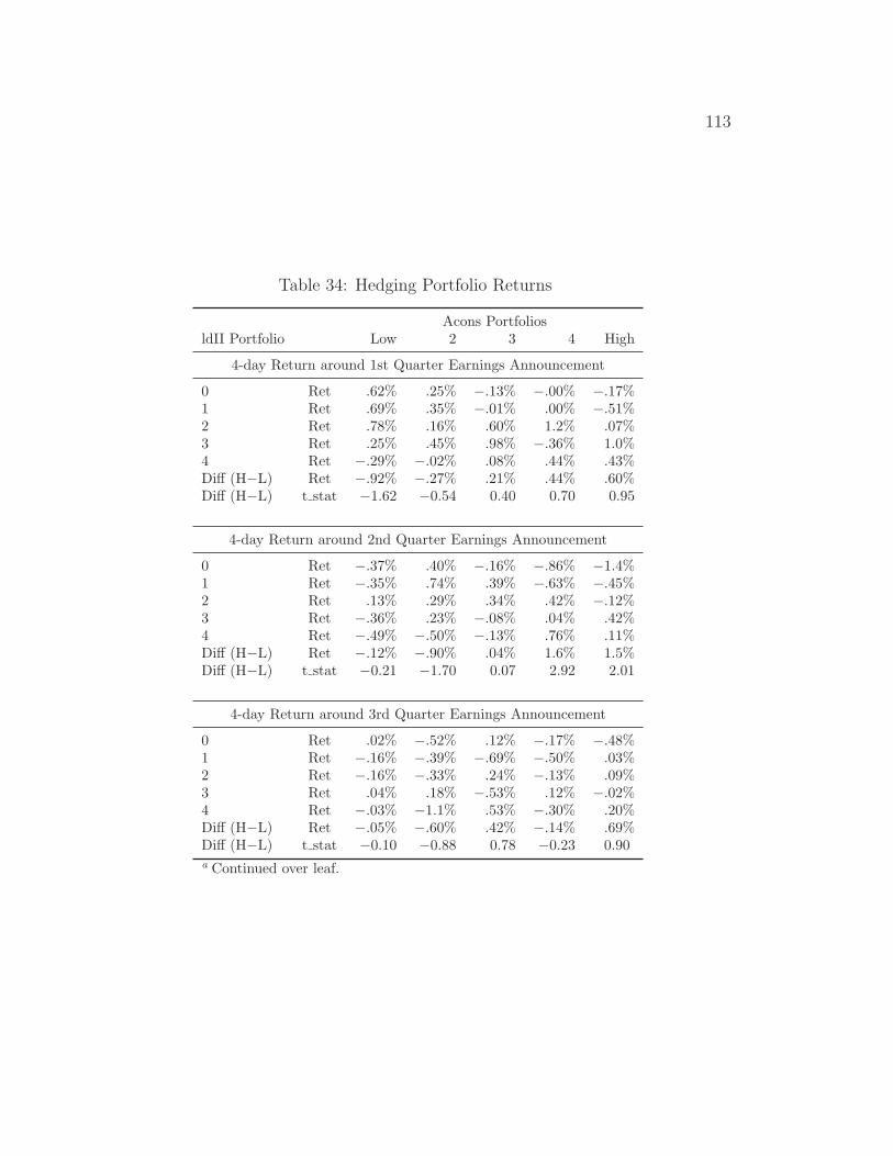
113

Table 34: Hedging Portfolio Returns

Acons PortfoliosldII Portfolio Low 2 3 4 High

4-day Return around 1st Quarter Earnings Announcement

0 Ret .62% .25% −.13% −.00% −.17%1 Ret .69% .35% −.01% .00% −.51%2 Ret .78% .16% .60% 1.2% .07%3 Ret .25% .45% .98% −.36% 1.0%4 Ret −.29% −.02% .08% .44% .43%Diff (H−L) Ret −.92% −.27% .21% .44% .60%Diff (H−L) t stat −1.62 −0.54 0.40 0.70 0.95

4-day Return around 2nd Quarter Earnings Announcement

0 Ret −.37% .40% −.16% −.86% −1.4%1 Ret −.35% .74% .39% −.63% −.45%2 Ret .13% .29% .34% .42% −.12%3 Ret −.36% .23% −.08% .04% .42%4 Ret −.49% −.50% −.13% .76% .11%Diff (H−L) Ret −.12% −.90% .04% 1.6% 1.5%Diff (H−L) t stat −0.21 −1.70 0.07 2.92 2.01

4-day Return around 3rd Quarter Earnings Announcement

0 Ret .02% −.52% .12% −.17% −.48%1 Ret −.16% −.39% −.69% −.50% .03%2 Ret −.16% −.33% .24% −.13% .09%3 Ret .04% .18% −.53% .12% −.02%4 Ret −.03% −1.1% .53% −.30% .20%Diff (H−L) Ret −.05% −.60% .42% −.14% .69%Diff (H−L) t stat −0.10 −0.88 0.78 −0.23 0.90a Continued over leaf.

114

Table 34: Hedging Portfolio Returns (continued)

Acons PortfoliosldII Portfolio Low 2 3 4 High

4-day Return around 4th Quarter Earnings Announcement

0 Ret .47% 1.1% .52% .42% −1.3%1 Ret .31% .49% .60% −.23% −.35%2 Ret .58% 1.3% .36% .56% .08%3 Ret .60% −.09% −.12% .89% .73%4 Ret −.44% −.01% .89% .26% .31%Diff (H−L) Ret −.91% −1.2% .36% −.17% 1.6%Diff (H−L) t stat −1.19 −2.14 0.57 −0.30 2.75

Sum of all 4-day Returns around Quarter Earnings Announcements

0 Ret 1.5% .29% −1.0% .85% −3.4%1 Ret .37% 2.0% .55% −1.3% −1.5%2 Ret 1.1% .97% 1.1% 1.4% 1.2%3 Ret .95% 1.0% .56% 1.1% 2.5%4 Ret −.28% −1.1% .83% 1.5% 1.3%Diff (H−L) Ret −1.8% −1.4% 1.8% .63% 4.6%Diff (H−L) t stat −1.62 −1.29 1.75 0.41 2.91a Each year firms are first sorted into quintiles based on averagepast conservatism score (Acons). For each Acons portfolio, firmsare further sorted into quintiles based on the change in investmentintensity (dII). For each of the 25 portfolios, returns arecomputed as returns over a 4 day window around subsequentquarterly earnings announcements (-1d to +2d) in excess of thevalue weighted market portfolio. The table shows portfolio excessreturns averaged over all years and the difference between thehighest and lowest dII portfolio.

115

Table 35: Portfolio Regression on Analyst Sales Forecast Errors

SalErrt = β0 + β1dIIt−1 + Controlst−1 + ...+ ut


Low −.062 −.035 −.098 −1.04 0.006 0.257 −.008 −.247 0.009 −.017 −.104 −.001 10.35% 958( 0.04) ( 0.03) ( 0.07) ( 0.82) ( 0.00) ( 0.08) ( 0.02) ( 0.15) ( 0.02) ( 0.02) ( 0.05) ( 0.00)

* *** *

2 0.015 0.005 −.033 −1.97 0.003 0.207 −.009 0.163 −.043 0.008 −.051 −.001 10.80% 1045( 0.03) ( 0.02) ( 0.06) ( 0.62) ( 0.00) ( 0.07) ( 0.02) ( 0.10) ( 0.02) ( 0.02) ( 0.05) ( 0.00)

*** ** *

3 0.016 −.005 −.109 −.228 0.000 0.275 0.062 0.039 −.037 0.003 −.151 0.001 9.77% 1168( 0.08) ( 0.04) ( 0.06) ( 0.70) ( 0.00) ( 0.09) ( 0.02) ( 0.08) ( 0.04) ( 0.01) ( 0.04) ( 0.00)

*** ** ***

4 0.021 0.019 −.130 −.890 −.002 0.335 0.012 0.078 −.030 0.005 −.043 0.001 11.14% 1108( 0.05) ( 0.03) ( 0.09) ( 0.50) ( 0.00) ( 0.07) ( 0.02) ( 0.09) ( 0.03) ( 0.02) ( 0.02) ( 0.00)

* ***

High −.091 0.051 −.062 −.043 0.007 0.255 0.010 0.008 −.001 0.010 −.020 0.002 10.55% 924( 0.04) ( 0.03) ( 0.09) ( 0.28) ( 0.01) ( 0.05) ( 0.03) ( 0.03) ( 0.02) ( 0.01) ( 0.05) ( 0.00)

** *** *

a Numbers in parenthesis are two-way clustered standard errors. *** denotes coefficients that are significantlydifferent from zero at the 1% level, ** denotes coefficients significant at the 5% level and * at the 10% level.Portfolios are quintiles based on firm-year realizations of Acons, which is the average degree of conservatismover the past 3 years. Forecast Revisions are computed as the difference between the most recent consensusbefore last year’s earnings announcement and the most recent consensus after last year’s announcement. SeeFigure 2 for details. dII = (II −GeoII)/|GeoII| with II = Inv/sale. ldII is lagged changes in investmentintensity. See appendix A for remaining variable definitions.

116

Table 36: Portfolio Regression on Analyst Pre-Tax Forecast Errors

PreTaxErrt = β0 + β1dIIt−1 + Controlst−1 + ...+ ut


Low −.773 −.179 −.530 −5.66 0.040 2.973 −.073 0.903 0.124 −.014 −.252 0.000 18.95% 629( 0.22) ( 0.13) ( 0.23) ( 6.91) ( 0.01) ( 0.44) ( 0.12) ( 1.13) ( 0.16) ( 0.08) ( 0.30) ( 0.00)

*** * *** ***

2 −.403 0.251 −.296 −6.71 0.046 2.716 0.048 1.385 −.252 −.067 0.001 −.000 14.69% 719( 0.29) ( 0.16) ( 0.44) ( 4.68) ( 0.03) ( 0.42) ( 0.23) ( 1.26) ( 0.13) ( 0.14) ( 0.32) ( 0.01)

*** *

3 −.359 0.004 −.705 −5.39 0.016 1.642 −.051 −.155 0.015 −.151 −.135 0.005 11.39% 780( 0.22) ( 0.18) ( 0.31) ( 5.09) ( 0.02) ( 0.33) ( 0.11) ( 0.36) ( 0.11) ( 0.06) ( 0.23) ( 0.01)

* *** **

4 −.102 0.072 −.615 −.545 0.002 1.503 −.007 0.154 −.120 0.006 −.074 0.004 6.57% 765( 0.16) ( 0.11) ( 0.47) ( 2.72) ( 0.02) ( 0.23) ( 0.18) ( 0.54) ( 0.12) ( 0.05) ( 0.09) ( 0.00)

***

High 0.050 0.243 −.163 0.115 0.002 0.814 −.085 −.006 −.297 −.148 0.016 0.012 5.68% 741( 0.28) ( 0.11) ( 0.25) ( 1.92) ( 0.02) ( 0.15) ( 0.10) ( 0.04) ( 0.12) ( 0.05) ( 0.15) ( 0.00)

* *** ** ** **

a Numbers in parenthesis are two-way clustered standard errors. *** denotes coefficients that are significantlydifferent from zero at the 1% level, ** denotes coefficients significant at the 5% level and * at the 10% level.Portfolios are quintiles based on firm-year realizations of Acons, which is the average degree of conservatismover the past 3 years. PreTax forecast errors is PreTaxErr = (Actt − PreTaxFCt)/|actt|, where PreTaxFCis the consensus PreTax forecast from IBES, computed in the same way as the earnings consensus forecast.dII = (II −GeoII)/|GeoII| with II = Inv/sale. ldII is lagged changes in investment intensity. See appendixA for remaining variable definitions.

Essays on Financial Information Analysis - Project...

Documents

Transcript of Essays on Financial Information Analysis - Project...