Essays on Inventory, Pricing and Financial Trading

Strategies

by

Ye Lu

Submitted to the the Sloan School of Management

MASSACHUSETTS INSTrtITEOF TECHNOLOGY

OCT 0 1 2009

LIBRARIES

in partial fulfillment of the requirements for the degree of

Doctor of Philosophy in Operations Research

at the

MASSACHUSETTS INSTITUTE OF TECHNOLOGYARCHIVES

September 2009

@ Massachusetts Institute of Technology 2009. All rights reserved.

Author .....................................................the Sloan School of Management

July 17, 2009

/2

Certified by .....................David Simchi-LeviDavid Simchi-Levi

Professor of Engineering Systems DivisionThesis Supervisor

Accepted by............Dimitris Bertsimas

Co-director, Operations Research Center

Q-,

Essays on Inventory, Pricing and Financial Trading Strategies

by

Ye Lu

Submitted to the the Sloan School of Managementon July 17, 2009, in partial fulfillment of the

requirements for the degree ofDoctor of Philosophy in Operations Research

Abstract

In a multi-product market, if one product stocks out, consumers may substitute to competingproducts. In this thesis, we use an axiomatic approach to characterize a price-dependent de-mand substitution rule, and provide a sufficient and necessary condition for demand modelswhere our demand substitution rule applies. Our results can serve as a link between the pric-ing and inventory literature, and enable the study of joint pricing and inventory coordinationand competition. I demonstrate the impact of this axiomatic approach on the joint pricingand inventory coordination model by incorporating the price-dependent demand substitutionrule, and illustrate that if the axiomatic approach is acceptable, the optimal strategy andcorresponding expected profit are quite different than models that ignore stockout demandsubstitution. I use this price-dependent demand substitution rule to model the joint pricingand inventory game, and study the existence of Nash equilibrium in this game.

In the second part of this thesis, I consider the problem of dynamically trading a securityover a finite time horizon. The model assumes that a trader has a "safe price" for thesecurity, which is the highest price that the trader is willing to pay for this security in eachtime period. A trader's order has both temporary (short term) and permanent (long term)impact on the security price and the security price may increase after the trader's order,to a point where it is above the safe price. Given a safe price constraint for the currenttime period, I characterize the optimal policy for the trader to maximize the total numberof securities he can buy over a fixed time horizon. In particular, I consider a greedy policy,which involves at each stage buying a quantity that drives the temporary price to the securitysafety price. I show that the greedy policy is not always optimal and provide conditions underwhich the greedy policy is optimal. I also provide bounds on the performance of the greedypolicy relative to the performance of the optimal policy.

Thesis Supervisor: David Simchi-LeviTitle: Professor of Engineering Systems Division

Acknowledgments

First and foremost, I would like to express my deepest gratitude to my advisor Professor

David Simchi-Levi, who has been not only a thesis advisor but also a cordial friend and

mentor to me. I learned a lot from David and enjoyed very much working with him. His

encouragement and support helped me tremendously through my years at MIT. He was the

reason why I came to MIT. He is the one who makes MIT more memorable to me.

I would also like to thank to Professor Stephen Graves and Professor Asuman Ozdaglar,

the other members of my thesis committee, for their time, effort and support to me.

To me, the ORC has been a great place, where I have met many classmates and friends.

I want to thank to them for making my life more enjoyable in the past three years.

Finally, I want to give my appreciation to Xiaoling for her love and support to my career,

and to my son, Zhongyu whom I should have spent more time with.

Contents

1 Introduction

1.1 Demand Substitution: Motivation . ...........

1.2 Demand Substitution: Literature Review . . . . . . . .

1.3 Demand Substitution: Contributions . .........

1.4 Adaptive Safe Price: Motivation and Literature Review

1.5 Adaptive Safe Price: Contributions . ..........

2 A Price-dependent Demand Substitution Rule

2.1 Deterministic Model . ..... .........

2.1.1 Demand model type I . . . . . . . ...

2.1.2 Demand model type II . . . . . . . . ..

2.1.3 Demand model type III . . . . . . . ..

2.2 Demand Sensitivity and System Demand . . . .

2.3 Summary . . . ....................

3 Joint Pricing and Inventory Coordination

3.1 Stochastic Model ..............

3.2 Comparisons Between Two Models . . . .

3.3 Summary ...................

4 The Joint Pricing and Inventory Game

4.1 An Extension in the Pricing Game . . . .

4.2 Existence of Nash Equilibrium in the Joint Pricing and Inventory Game . ..

11

... ... 11

. . . . . . 12

. . . . . . 12

. . . . . . 13

.. . . . 14

17

.. . . . . . 17

.. . . . . . 19

. . . . . . . . 22

. . . . . . . . 30

. . . . . . . . . . 33

.. . . . 37

39

.. . . . 39

.. . . . . 41

. .. .... . 46

49

50

55

4.3 Summary ..................................... 63

5 Adaptive Safe Price 65

5.1 Greedy Policy is Not Always Optimal ................... ... 67

5.2 When is Greedy Policy Optimal? . . ........... . .... ...... . . 69

5.3 Lower Bound for Greedy Policy ......................... 75

5.4 Summary ............. ....................... 78

6 Conclusion and Future Research 79

List of Figures

3-1 product 1's demand ................................

3-2 CDF for product 1 demand under the two models when Y2 = 3, pi = 226 and

p 2 = 219 . . . . . . . . . . . . . . . . . . . . . . . . . . . . . . . . . . . .

4-1 7r1(pl, 40, 6) ....................................

4-2 p*(P2)

5-1

5-2

5-3

5-4

5-5

The law of price motion . ............

Greedy policy fails . ...............

First case that greedy policy is optimal.....

Second case that greedy policy is optimal.

Optimal regions for No-buy and greedy policy.

.. . . . . . . . . 66

.. . . . . . . . . 68

. . . . . . . . . . 74

. . . . . . . . . . 75

. . . . . . . . . . . . . 76

List of Tables

3.1 Difference on the strategy and profit ... ................ ... 43

3.2 More is not always better! . . . . . . . . . . . . . . . . . . . . . . . . . . . 45

Chapter 1

Introduction

In this thesis, we consider operational problems in face of uncertainty. One problem is in

the area of supply chain management focusing on the coordination of inventory and pricing

strategies when competition exists. The second problem deals with investment challenges

faced by large institutions whose investment may affect market price.

1.1 Demand Substitution: Motivation

The coordination of pricing and inventory decisions is challenging, in particular in an envi-

ronment where the firm has substitutable products. In such an environment, the price of one

product affects not only its own demand but also the demand of other products. At the same

time, since products are substitutable, demand for some products may increase, when other

products stockout. Unfortunately, the operations management literature on multi-product

inventory and pricing coordination, that takes into account both effects, does not exist.

To illustrate the challenge, consider a retailer with substitutable products such as Pepsi

and Coke. Some consumers may switch from one product to another either due to a change

in price or during a period of stockout of one of the products. In fact, in both cases, the

number of customers switching to another product depends on all (or remaining) product

prices.

1.2 Demand Substitution: Literature Review

In recognition of these challenges, the literature in this area can be divided into two cate-

gories. In the first, see for example, Aydin and Porteus[3], Birge et al [6] and Maddah and

Bish [19], price is a decision variable but customers do not switch during stockout periods.

In the second, see for example Van Ryzin and Mahajan [28], Smith and Agrawal [29] and

Rajaram and Tang [26], prices are assumed to be exogenous and customers switch during

stockout period according to a price-independent substitution rule.

A similar challenge exists in a decentralized system, where multiple retailers compete

simultaneously on pricing and inventory. As a result, the literature here can also be classified

into two categories. In one, demand is independent of price, and competition is on inventory,

see Parlar [24], Lippman and McCardle [15], Mahajan and Van Ryzin [21] and Netessine and

Rudi [22]. In the second, see Bernstein and Federgruen [8] and Chen et al [10], demand is a

function of price and competition is on price but not on inventory.

1.3 Demand Substitution: Contributions

The literature review suggests that the coordination (and competition) of pricing and inven-

tory decisions in an environment with multiple, substitutable products (or identical products

offered by multiple retailers) remains an important challenge. This is due to the lack of price

dependent substitution rule, that is a rule that suggests how consumers switch from one

product (retailer) to another as a function of price during periods of stockout. This is ex-

actly the objective of this thesis. Specifically, I use an axiomatic approach to characterize a

price-dependent demand substitution rule.

The basic question I address is as follows: Given a specific demand model for n products,

what is the impact of removing a subset of the products from the system on the demand of

the other products. Remarkably, I show that under general demand models, it is possible

to exactly characterize customer demand for the remaining products. The approach used

in our analysis is an axiomatic one, that is, I make no assumption on the structure of the

demand model for the remaining products and show that there is a unique price-dependent

demand substitution rule to determine the remaining products demand model. Our demand

models are general, and include the Linear model, the Attraction model, the Logit model and

the CES model as special cases. This part of work in done in Chapter 2. In Chapter 3, I

apply this result to a joint pricing and inventory coordination model, and demonstrate the

impact of our substitution rule on the optimal inventory and pricing strategy. In Chapter 4,

I use the price-dependent demand substitution rule to model the joint pricing and inventory

game, and study the existence of Nash equilibrium in this game.

1.4 Adaptive Safe Price: Motivation and Literature

Review

In the second part of this thesis, I consider the problem of dynamically trading a security

over a finite time horizon. Given the dramatic increase in institutional trading in recent

years, there has been much interest in the optimal control of the execution costs. During the

last few years, several studies have been done on dynamic optimal trading strategies that

minimize the expected cost of trading a security. Specifically, a trader has to buy Q units of

a security over N + 1 periods. Let qi denote the trade size for the security at period i. Then

this problem can be expressed as:

minqiE{ iNoPii} (1.1)

s.t. Ei=oq i = Q. (1.2)

In each period, the price of the security is a function of the trader's order size. The law

of motion for price pi may be expressed as

pi+1 = pi + 0qi + ei, (1.3)

where 0 is a positive constant and ci is a random variable. This model first appeared in

Bertsimas and Lo [9]. They show that to minimize expected execution cost, a trader should

split his orders evenly over time. Almgren and Chriss [2], Huberman and Stanzl [13] and

Schied and Schneborn [30] extend the Bertsimas and Lo framework to allow risk aversion and

temporary price impact. Obizhaeva and Wang [23] and Alfonis, Schield and Schulz [4] model

the dynamics of supply/demand in a limit-order-book market and allow continuous trading.

I also refer the reader to Almgren [1] and Alfonis, Schield and Schulz [5] for nonlinear price

impact model and Moallemi, Park and Van Roy [20] for trading in a competitive setting.

1.5 Adaptive Safe Price: Contributions

In Chapter 5, I consider the case when the trader identifies a "safe price", P, for the security.

Although the trader can not predict the exact price of this security after N + 1 periods, he

is confident that the security's price should be somewhere above this safe price. Therefore,

as long as the trader purchases this security at a price below the safe price, he will be able

to profit at the end of the time horizon.

At the same time, this safe price, P, also represents the trader's risk aversion level, which

means that p is the highest price that the trader is willing to pay for this security. Suppose

the trader has a budget (available cash in hand), Q, for this security. Given that the trader

will profit at the end of the planning horizon as long as this security is bought below the

safe price, the trader can adopt a strategy that maximizes the total number of securities

purchased over the N + 1 periods. If at some time period, the trader runs out of cash, then

he can stop. If at the end of last period, there is still some cash left, the trader at least has

bought as many units as possible below the safe price p, which maximizes the profit he can

make under the assumption that the security's price will be somewhere above this safe price.

Traders can adjust their safe price at the beginning of each period. For example, at the

beginning of period i, the trader has observed the security's current price and its price motion

over the last i periods. Given these observations, the trader may re-predict the security's

price and adjust its safe price from pi-1 to Pi.

It is tempting to conclude that since the trader's goal is to maximize the number of units

of security, the trader should purchase to increase price up to Pi. I refer to this policy as

the greedy policy. Unfortunately, I show in Section 5.1, using a counter example, that the

; ;__ .~1 _ _^_~__ ______~ _ l___//l;(;_jl__; _~;;;;___~_________;_^_i

greedy policy is not always optimal. The following questions are therefore natural: What is

the structure of the optimal policy? Under what conditions the greedy policy is optimal?

And, when it is not optimal, how far is it from the optimal? These questions are answered

in Chapter 5.

Chapter 2

A Price-dependent Demand

Substitution Rule

This chapter is organized as follows. In Section 2.1, we present and prove the price-dependent

demand substitution rule for deterministic model. In Section 2.2, we use the demand sub-

stitution rule to study how demand sensitivity and system demand depend on the number

of products.

2.1 Deterministic Model

Consider a market with n products indexed by i = 1, 2,..., n. Let

D = (dl,..., dn) T = demand vector (2.1)

p = (pl,...,pn)T = retail price vector (2.2)

The demand for each product depends not only on its own retail price, but also the retail

prices of the other n - 1 products. We assume that the n products are substitutable, so that

if the retail price for product i is increased, not only will the demand for the i's product

decrease, but also the demand for the other products, other than i, will increase.

Thus, we assume that the demand models always satisfy the following assumption.

Assumption 2.1.1. The demand functions di(p), i = 1,..., n are continuously differen-tdi (p) dj (p) > otiable, , < 0 and p> , j i.

In this section we answer the following question. Given n competitive products having

demand according to demand model D, what is the impact of removing m of the products

on customer demand for the remaining n - m products?

In the analysis below, we denote = {m + 1, .. ., n} and -R = {1,..., m}. For any

set F E R n , we let fl-_ F and fl, F be the projection of F onto its first m variables and

last n - m variables, respectively. Without loss of generality, we assume that we remove

the product indexed by 1, 2,.. ., m from the system, and our objective in this section is to

determine the demand for the remaining n-m products. To answer this question, we assume

that the demand for the remaining n - m products should satisfy the following two basic

assumptions. Let dq(pR), j E R be the new demand function for each remaining product.

Assumption 2.1.2.

(a) If a subset of products with positive demand is driven out of the market, the demand for

each remaining product does not decrease.

(b) If all products i, with i -R are removed at some price vector (p_g,pR) such that

di(p-, pj) = 0, for each i e -R, the demand for each remaining product j, j E R, does not

increase.

The first assumption is not valid for complementary products, such as PCs and Laser

Printers; when one is removed, we expect a decrease in the the demand for the other.

However, this assumption is valid for substitutable products since when some products are

removed from the market, there is no reason that the demand for remaining products will

decrease. Formally, the assumption can be written as follows: For any fixed pR, we denote

F_,_ = {p_~ E Rmld_g(p-_,pg) 0}, SR = {p-R E RlJd_(p-_,pa) = 0} and 7_- =

F-R \ S-a. The first assumption implies that

--- ----- --- _ _F_

dR(pe) > max dj(p_g,pj), JE R. (2.3)

The second assumption suggests that if no customer is willing to buy from products

1, 2,..., m at a certain price vector (p_, p_), removing these products from the market

won't increase the demand for the other products. Of course, removing products i, i E -R

may increase the demand for the remaining product j, j C R, when customers who would

have purchased products i, i G -R, switch to buy the remaining product j,j E R after

the removal of -R. But this won't happen if there is no customer demand for products

i, i E -R. Formally, the second assumption implies that

d '(pR) < min dj(p_-,p~), j C . (2.4)P-- ES_a

Thus, under the above two assumptions, we have for any demand model

max dj(p-R,pR) < d(pR) < min d (p_R,pR), j E R, (2.5)pREr- -- ES_

Our objective is to characterize conditions under which the lower bound (2.3) and upper

bound (2.4) match, i.e,

max dj (pR, p) = min dj(p_, p), j E RJ, (2.6)p_Er- pwES_

which implies that the demand function for the remaining products dq(pR), j E R is uniquely

determined. For this purpose, we partition the set of demand models satisfying Assumption

2.1.1 into three types.

2.1.1 Demand model type I

For type I demand model, we assume that demand for a subset of the products is zero only

when price for these products is infinite.

Assumption 2.1.3. di(p) > 0 for any p E Rn+, and di(p) = 0 when pi = oo, i = 1,..., n.

The following demand functions satisfy this assumption.

Attraction Models. Attraction models are among the most commonly used market

share models. The market demand achieved by a given firm i is given by its attraction value

divided by the industry's total value, i.e,

di(p) = M U ) (2.7):N=o Uj (p)

Here M is the fixed market size, u0o is a constant and Ui(p) = kip ai or uj(p) = ke - aiPi

for constants aj, ki > 0.

Logit Model.

di (p) k (2.8)E=1 k-e- \Pj

with A > 0 and ki > 0 for all i.

CES Model.

r-1.

di(p) - iP (2.9)

with r < 0 and 7 > 0.

For type I demand model, Assumption 2.1.1 implies that maxp_,,r_ dj(p_a,pw) =

dj(00,pR) because dj(p_g,pW), j E R increase with p_g. Assumption 2.1.3 implies that

minp_cs_a dj(p_, pg) = dj(oo, p) because infinity is the only point in S_a. Therefore,

for Type I demand model, equation (2.6) holds and the demand functions for remaining

products are uniquely determined by d (pR) = dj(oo, pg), j E .

Observe that for any pR, infinity is the solution to d-_(p_,, pR) = 0, i.e., the price vector

such that the demand for removed products is zero. This implies that the the price-dependent

demand substitution rule can be described as follows:

Price - dependent Demand Substitution Rule : For any pR, let p*(pz) be the solution

to dg(p_--, p) = 0, i.e., the price vector such that the demand for removed products is zero,

then demand function for remaining products is

d-(pa) = dj(p* (p J),p), j .. (2.10)

An intersting question is whether this demand substitution rule, determined by equa-

tion (2.6), is appropriate for other type of demand models, beyond Type I demand model.

Unfortunately, we face important challenges once we try to extend beyond Type I demand

models, as is illustrated by the following examples.

Example 2.1.1. Let

dl(pl,p 2,p3 ) =

d 2 (P1 , P2, P3 ) =

d3 (pl,p 2,p 3 ) =

and notice that these demand functions

that the solution to the following system

di(pl, p2, 1)

d2 (pl,p 2 , 1) =

9 - pi + (P2 - 20)1 + P3,

9 + pi - P2 +P3,

9 + Pi + P2 - 2p3, (2.11)

satisfy Assumptions 2.1.1. Set pa = 1 and observe

1

10 - pi + (p2 - 20 ) 5 = 0,

10 + p -p2 = 0,

S_, consists of three points, (9, 19), (10, 20) and (11, 21). Since we have three values of

p*__(pe), it is not clear any more which one shall we assign into equation (2.10)? We call

this the uniqueness problem.

Even if S-_g consists of only one element, it can happen that the resulting demand model

does not make practical sense.

Example 2.1.2. Consider the following demand model

2 3di(pI,p 2,p 3) = 2 0 0 -pl+ -P2 -+ P3,5 5

1 3d 2(plp 2,p 3 ) = 164+ p1 -p2 p3.

2 51 1

d3 (P1, 2, P3) - 150 + pl + IP2 -P32 2

Notice that these demand functions satisfy Assumptions 2.1.1 and for any p3, P*-_(p 3)

(332 + 2P 3, 330 + 9p3). Hence, removing product 1 and product 2 yields a new demand

function for product 3 satisfying,

7d"(p) = d2 (P*(P 3), 3) = 481 + PS3 . (2.12)

80

This implies that product 3's demand increases with its own price. We call this the consis-

tency problem.

To address the uniqueness and consistency problem, we study the following type of de-

mand model.

2.1.2 Demand model type II

Denot-e-- {p E R di(p) > 0}. For type I demand model, F = Rn+. As you will see, this

is not true in this subsection. Therefore, in this subsection we only consider the region F.

Recall H.I F is the projection of F onto its last n - m variables. For demand model type II,

we assume that the demand functions satisfy the following property.

Assumption 2.1.4. For any fixed pgz E fJ F, there exists finite p* RG R' such that

(p*_, pR) C F and d_-(p*R, pg) = 0.

This assumption implies that given a price vector pW for a subset of the products R,

there is only finite price vector p*_ satisfying d-_(p*_, p) = 0. Both Example 5.1.1 and

Example 2.1.2 satisfy Assumption 2.1.4. Therefore, to solve the uniqueness and consistency

problem for type II demand model, we need to replace Assumption 2.1.1 by a slightly stronger

assumption. Before we describe this assumption, we need to introduce the notation of M-

matrix.

Definition 2.1.1. A square matrix A is called M-matrix if all off-diagonal entries are less

than or equal to zero and it satisfies any one of the following equivalent conditions.

(a) All principal minors of A are positive.

(b) The leading principal minors of A are positive.

(c) The diagonal entries of A are positive and AH is strictly diagonally dominant for some

positive diagonal matrix H.

(d) A is non-singular and the inverse of A is non-negative.

For more details on M-matrix, see [12, §2.5]. We denote the Jacobian matrix of the

demand functions by

Sadi (p) di (p)

J = "" . (2.13)

Odn (p) adn (p)

We replace Assumption 2.1.1 by the following assumption.

Assumption 2.1.5. -J is an M-matrix.

Notice that Assumption 2.1.5 implies Assumption 2.1.1 because all off-diagonal entries

of -J, ad(p) 0, j Z i, and Definition 2.1.1 part (c) implies that its diagonal entries,

di(p) > 0.api

At a first glance, Assumption 2.1.5 looks quite technical. However, we show that this

Assumption is more general than both of the following, commonly used assumptions, for

multi-product demand models.

Assumption 2.1.6. adi(p) < - ai(p n.api < apj, 2 ,...,n.

Assumption 2.1.7. di (P) - i dj(p), i = n.ap < apin

Assumption 2.1.6 implies that if all products' prices increase by the same amount, the

demand for each product will decrease. Assumption 2.1.7 implies that a price increase by

any one of the products results in a decrease of total sales in the market. To see that

Assumption 2.1.5 is more general than Assumption 2.1.6, Assumption 2.1.6 is equivalent to

setting H = I, the identity matrix, in part (c) of Definition 2.1.1. Assumption 2.1.5 is more

general than Assumption 2.1.7 because if a matrix is an M-matrix, its transpose is also an

M-matrix.

In the rest of this section, we show that (i) Assumption 2.1.5 solves the uniqueness prob-

lem, i.e, for any pR, the solution to d_W(p_, pR) = 0 is unique; (ii) Assumption 2.1.5 solves

the consistency problem, i.e., demand functions dq(pw), j E R obtained by our demand

substitution rule (2.10) satisfy Assumptions 2.1.4 and 2.1.5; (iii) under Assumption 2.1.5,

equation (2.6) holds. Therefore, dq (pR) = dj(p_ (pR), pW), j c R. are the only demand func-

tions that satisfy Assumption 2.1.2; (iv) Assumption 2.1.5 is not only a sufficient condition

for (i),(ii) and (iii) to hold, but also a necessary condition for (i) and (ii) to be true.

Consider the linear demand model,

D = b - Ap, (2.14)

where the constant vector b is the expected demand if the prices of all the products are set

zero. Therefore, b must be positive. It is easy to see that if the linear demand model satisfies

Assumption 2.1.5, it also satisfies Assumption 2.1.4. Notice that if A is an M-matrix, its

sub-matrix A_s~ is also an M-matrix. We write A = . Therefore, for anyA3 Az)

fixed pR e R - , p*t = A- (b - A 2 * PR) > 0, and hence for the linear demand model, the

solution to d_ (p-_, pR) = 0 is unique for any fixed pR.

Generally, a system of nonlinear equations can have multiple or even positive dimensional

solutions. Interestingly, it has been shown in Gale and Nikaido[11] that for any nonlinear

functions that satisfy Assumption 2.1.5, there is at most one solution to d a(pR, pg) = 0.

For completeness, in what follows we introduce a method to address both the uniqueness

problem and the consistency problem.

Consider the region F. For any fixed pw E nJ, F, define F_- = {p-a e Rm (p_a,pa) E

F}. Let R(2) = {2,...,m}, we know that for any pR(2) E R(2) -R, the projection of

F_- onto its last m-1 variables, Assumption 2.1.4 ensures that there exists pi such that

i:i:-"~;"~l~~"~l~%--~---~--(i-Y -- n; :

dl(pl, pR(2), pR) = 0 because (pR(2), pW) E HR(2) U F. Notice that di(pl, pR(2), pR) = 0 can have

only one solution because d(p) < 0 from Assumption 2.1.1. Therefore, dl( (p), p(2)) = 0

defines a function from H(2) F- to R+ by

(2.15)

After submitting this function into dj(pR, pR), we get

dS2) (pW(2) , pZ) = dj (pl (p(2)), pg(2), pg),

We claim that d 2 ) (p(2), pZ) has following properties.

Property 2.1.1. If p*_ E F-a is a solution to d_-(p_, pa) = 0, then d (2)

- , 'R(2) (p*(2), pA) = 0.

Property 2.1.2. For any fixed pRu() E h(j) F- with R~() = {j, j + 1,..., m}, there exists

P (2)\,j) such that (p (2)\(j), P(j)) H(2) F-, and (2)\ (j) (P*(2)\R(j),) Pi (j), P) = 0.

Property 2.1.3. -

d2) (p)ap2

ad()aOdPOP2

ad2) (p)

• iis an M-matrix.

Od( ) (P)Opm

Proof. Property 2.1.1 follows from the definition of d (2) (p(2), pp). If d_-(p* , pR) = 0, then

d(2) (P*(2),p) = d( 2) (p 1(2) p(2) p, p) = 0. Property 2.1.2 follows from Assumption 2.1.4

and Property 2.1.1. Next, we prove Property 2.1.3. From the definition of pi(pg(2)), we must

have dl(pI (pR(2)), P~(2), p~) = 0. Implicit function theorem tells us that

apl1(P(2)

api

adl(p)

adi (p) 'api

i E (2) (2.17)

Therefore, we get

j E R(2) (2.16)

Pi = Pl (p(2)).

&di (pl (p(2)), pg(2), PWR)

OpiOdi (p) aPI(PR(2))

9p7 Oapi

Odi(p) odi (p)Dpi

9p1 odi (p)(9p1.

det (

aOd (p)._[ P -

where the last inequality follows from part (a) of Definition 2.1.1. For i, j E R(2) and j = i,

Odi (p) aGp(pg( 2))

ap 1 apj+di (p)+- op)

( dl (p)adi (p) a di(p)

9p,1 dl (p) + pjdi (p)apj

Notice that if a matrix is an M-matrix, its principle sub-matrix is also an M-matrix.

Therefore, part (c) of Definition 2.1.1 implies that there are positive constants Ai, i

1,..., m such that

j adi(p)- A p > 0, (2.19)

j=1 ap w

for any i = 1,..., m. Therefore, for any i = 2,..., m, we have

m Aj Odi(p)Odi (p) Ejm=2 \,10pj9 (p)Ozdl (p)

ap di(p)

Od (p)O 1

m

-Ej=2

Aj Odi(p)

A I pj

Im di(p) > ,

j=2

where the equality follows from (2.18), and the inequalities follow from (2.19).

(2.20)

Property

2.1.3 holds.

The following lemma reveals an interesting relationship between dR (p_, pR) and

d(2)c( (P-R2), Pg).

d (2) (p2), P )Opi

+di (p)api

-d l (p)

pi

&dl (p)Dpi

&di(p)9dl(P)i

Opi&di (p)

atp / <0, i E R(2)

> 0. (2.18)

--

-

-

.

.. .. ..

(2)ad,) (p(2) , p R)

opj

M Aj

Sj=2A,j= 2

Lemma 2.1.1. For any fixed pR E FIR F, denote FW(2) = {pR(2) E HR(2) F-ld )2)(p (2), pa) >

0} then FR(2) = HI(2) F--.

Proof. " C " follows from definition of F(2). Now we prove " 2 ". For any pR(2) E

HI(2) F -, by the definition of projection, there exists pt such that (p, pR(2)) e F-. There-

fore, we have di(p*,pJ(2), pR) > 0. Let pi = p1(pZ(2)) be defined by equation (2.15). Then

dl (pl (pg(2)), pJ(2), pR) = 0. From Assumption 2.1.5 we know dl(p) strictly decreases in pi, and

hence we must have pl((p_(2)) > pT. Assumption 2.1.5 also tells us that dR(2) (p) increases in pl.

Therefore, we have d(2) (p( 2), p) = dg( 2) (pl(pR(2), p(2) , p) > d( 2) (p*, p1(2), pR) > 0. This

implies that pR(2) E FV(2) and consequently fl(2) F-R C FR(2). Hence, FR(2) = (2) F. El

We can apply the same method to obtain d (j + l ) p p) by submitting p3 = pj (p+l)

(defined like (2.15)) into d(j) (pj, pj+, p), ip.e., d(j+) = (+)( ),

p(j+l),p), here R() = {j,j + 1,...,m}, j = 2,..., m. And by induction, we can show

that d( ,j) (paw(), p) has the same properties that d(2) (p?(c2) , pR) has. Therefore, Lemma 4.1

implies that FR(j+1) -= f (j+l) Fj), for F(j) = {p(I1)E R(j) F(j-,(1) (p(),p ) _ 0)

and j = 2,..., m with Fw(1) = F--.

We show uniqueness and consistency properties in the following theorem.

Theorem 2.1.3. Consider any demand model that satisfies Assumptions 2.1.4 and 2.1.5.

(a) (uniqueness) Given any fixed pg E fIR F, the solution of d_R(p-_, pR) = 0 is unique.

We denote it by p* (or p*i(pz) since it is uniquely determined by pR).

(b) (consistency) The demand functions obtained from the demand substitution rule, d'(pa)

= dj (pli(pR),pR), j e R, satisfy Assumptions 2.1.4 and 2.1.5.

Proof. (a) We prove by induction starting from the last element in the vector p*R.

Notice that d1 (pR(m), pa) consists of a single function with a single variable p,. From

Property 2.1.1, we know that for any p*R such that d-_(p*i,pR) = 0, d(r(p( (*pM)

0. From Property 2.1.3 we know da1) (p~( m ), p) = 0 can have only one solution becausead (pm),PR) < 0. Therefore, in the set {p* E R m d_(p* R, p) = 0}, the mth component,

pm, is unique.

p* , is unique.

We now apply the same idea to d(m- 1) (Pm-l, P*, pR) = 0 to obtain that the solution to

this equation is unique and hence Property 2.1.1 implies that the (m - 1)th component in

the set {p"* E Rm d_(p*, ,paz) = 0}, p-1_, is unique. Using induction, we have that the

kth component, p*, is unique for k = m - 2,... ,1. Therefore, there is only one p"* such

that d-(p-l, P ) = 0.

(b) Define '(j) = {j, j+ 1,... ,n}, j = 2,...,m+ 1, and d 2) (p,( 2)) = dj(pl(pR,(2)), P,(2)),

j E R,(2), here pl(p~,(2)) is the unique solution to dl(P1, pR,(2)) = 0. Then, applying exactly

the same method as the one used for proving Properties 2.1.1, 2.1.2 and 2.1.3, we can show

that d2) (p,(2)), j E R,(2) satisfies Assumptions 2.1.4 and 2.1.5. By induction, we know

dS +1) (p(m+l)), j E R'(m+) satisfies Assumptions 2.1.4 and 2.1.5.

The last step is to show that removing product one by one from the list of products

is the same as removing a group simultaneously. Indeed, the property that the solution to

d_-(p-, p) = 0 is unique for any fixed pR E 1, F implies that d(pR) = dj(p*(p),p ) =

d m+1) (p~,(m+)), j E R/(m+l). This completes the proof part of (b). ol

The Theorem thus implies that Assumption 2.1.5 completely addresses the uniqueness

and consistency problem. Next, we show that under Assumption 2.1.5, equation (2.6) holds.

For this purpose, we need some technical results that provide a different characterization of

of Assumption 2.1.4.

Theorem 2.1.4. For any fixed pR E nf F, there exists only finite p* E Rm such that

(p*", pa) E F and d-R(p*_, pR) = 0 if and only if F- is nonempty and bounded.

Proof. We first prove ">". Since di(p) strictly decreases in pi, for any (pl, pR(2) E F-R,

we must have Pi pl (pg(2)) to make di (p, pR(2) , pR) > 0. And since dl (pl (pI(2)), 1pg(2), pR) =

0, implicit function theorem implies that

ad i(p)OP1(p2)) - O, j (2). (2.21)

Opj adl (p)

api

Since Pi(PR(2)) increases in pR(2), F- is bounded if (2) F- is bounded. Lemma

4.1 shows that H,(2) F- = FR(2). Therefore, the original problem (proving that F-a

is bounded) is reduced to showing that Fa(2) is bounded. However, we have shown that

i----~~"-~-l--~" -~-"~ii""l"""~"~"~--~c :

d(2) (pZ(2), pR) has the same properties as of d_W(pR,pR), and so does d )(p(j ),P), i3,..., m. Therefore, by induction, this problem is reduced to showing that F ), is bounded.

Notice that d, ) (pg(m),pe) consists of only a single function with a single variable pm.

In the proof of Theorem 2.1.3, we have shown that these exists a unique pm such that

d(m) (p,* p,) = 0. Since d(m) (Pm, pR) strictly decreases in pm, we must have F-cm ) C [0, p*]

which is bounded. And consequently, F - is bounded.

Now we prove "". Since F-s _ is nonempty, there exists a po% E F-_. If dz(p g, pR) #

0, we construct a sequence starting from p0_ in the following way. We move from pOR to

pl by keeping all components of pO, unchanged except increasing (p°%)1 to (plR)1 such

that di(p", pR) = 0. From Assumption 2.1.1, we know that increasing (poR)1 will increase

the value of di(p), i = 2,..., n. Therefore, we are staying inside F-3 before violating the

nonnegativity constraint of di(p). Since F--_ is bounded, there must be a finite (p1W)1

such that di(p_,p) = 0. Applying the same technique, we obtain piR, i = 2,..., m such

that di(pi ,pa) = 0, i = 2,...,m. If we don't have d_ (p_,p,) = 0 after one round,

we start all over again by increasing (PI)1I to get pm+l such that dl(p , p+l e) = 0. If

this algorithm stops after finite steps with a p*g such that d _(p*_, p3) = 0, we achieve

our goal. Otherwise, we have a sequence {p y E F-g such that d(pkm+j,) = 0 for

j = 1,... , m and k = 0, 1,.... Notice that {(p' )j }-1 is a nondecreasing sequence for any

j = 1,..., m. It must converge to some point (p* )j. Therefore, {pi}--1 must converge

to P*. Since F- is bounded and closed (the closeness of F_- follows from the continuity

of di(p), i = 1,..., m), we must have pT* E F-. Moreover, we know that if a sequence

converges to a point, its subsequence must converge to the same point. Therefore, by con-

tinuity we have dj(p~,,pM) = limk,,o dj p ,p ) = 0 for any j = i,...,m. We have

d_R(p*_, pR) = 0. ol

Theorems 2.1.3 and 2.1.4 motivate the following important property of type II demand

model that plays a key role in our proof of equation (2.6).

Theorem 2.1.5. (bound) For any p_ E F -, we have p_M p*_,(pz), where pt_*(pR) is

the unique solution of d_R(p_1,pg) = 0 (defined in Theorem 2.1.3).

Proof. From Theorem 2.1.4, we know that for any demand model satisfying Assumption

2.1.4, FR is bounded. Therefore, for any p_ G F- _, if p_-a p*_ (P), we can construct

the same nondecreasing sequence starting from p_R as we did in the proof of Theorem 2.1.4.

The proof of this Theorem tells us that this sequence must converge to the solution to

d_-(p-_, pR) = 0. From Theorem 2.1.3, we know pI*(pg) is the only solution to this system

of equations. Therefore, this sequence must converge to p*i(pR). Since this is a nondecreas-

ing sequence, we must have p_ < pT_(pR). O

The Theorem thus implies that for any fixed pg, the unique vector p*_(pg) is an upper

bound (component by component) on any price vector p_ CE F- . Before we prove equation

(2.6), we first introduce our last type of demand model.

2.1.3 Demand model type III

This demand model is a combination of type I and type II demand models. It is characterized

by the following assumption.

Assumption 2.1.8. di(p) is well-defined at pj = oc, for i,j = 1,..., n. Part of these

demand functions satisfies Assumptions 2.1.1 and 2.1.3, the other part of these demand

functions satisfies Assumptions 2.1.4 and 2.1.5.

Notice that in type I demand model, for any fixed pa (can be infinity), p*(pa) = oo

has exactly the same properties (uniqueness and bound) as the p*(pg) defined in Theorem

2.1.3 for type II demand model. Therefore, we use the following theorem to summarize our

main results for all types of demand models.

Theorem 2.1.6. For any fixed pW, the solution of dj(p_,pW) = 0 is unique. We denote

this solution by p* g(pR) (it is infinity for type I demand model, defined in Theorem 2.1.3 for

type II demand model and a mixed solution consisting of infinite and finite components for

type III demand model). Then, for any p_g E F-R, we have p_ < pt*_(pe).

We are now ready to present our main result.

Theorem 2.1.7. Consider the three types of demand models defined in this section. For any

pj, we have

max dj(p_, p) = min dj(pR, pR), j E R. (2.22)pREF-_ pRESR

Therefore, removing all the m products in the set -R from the market creates a demand

function for the remaining n - m products that follows

d'(pg) = dj(p*g (p),p), j E ?, (2.23)

where p*(p) is defined in Theorem 2.1.6, and this is the ONLY demand function that

satisfies Assumption 2.1.2.

Proof. From Theorem 2.1.6, we know that for any pW, S-_ consists of only one el-

ement, p*_(p). Therefore, minp_es_ dj(p-,Pa) = dj(p*_(i ),p). We first prove

maxp_,Er_ dj(p_-,pR) dj(p ,(pR),pj). In the proof of Theorem 2.1.4, we know that

there is always a sequence {pki}k_1 c FR such that limko,, P* (pR) (this property

certainly also holds if p*(pR) = oc). Since dj (p) is continuous,

dj (p*~ (p ), p ) lim dj (pk,p4) < lim max dj(p_ ,pw)= max dj(p_-,pR). (2.24)k-oo k--op_-EF_- P-REF_r

From Theorem 2.1.6, we know that for any p_- E F-, p-a < p*R(pR). And since for any

j E R, dj(p_, pR) increases in p_,

max dj(pR,p-) < dj(p*pp~),pw),j E R. (2.25)

Therefore, we have maxp_,Er-, dj(p-r, pe) = d (p*=(pR),p) minp-es- di(P-,p)

Since the lower bound and upper bound of d?(p) match at dy(p*R(pp), pj), equality (2.23)

holds. Moreover, this is the only demand function that satisfies Assumption 2.1.2. Ol

Theorem 2.1.7 tells us that if the demand model satisfies Assumptions 2.1.4 and 2.1.5

(which is a subset of Assumption 2.1.1), then the new demand model is obtained by setting

the price of the removed products such that their demand is zero and this is the only possible

demand model.

We now prove that Assumption 2.1.5 is not only sufficient but also necessary. That is, we

show that if the demand model satisfies Assumptions 2.1.1 and 2.1.4, and the new demand

model is obtained by setting the prices of the removed products so their demand is zero,

then the demand model must satisfy Assumption 2.1.5.

Theorem 2.1.8. If a demand model, D ={d(pj(p),.... d,(p)},

and 2.1.4 and dq(pw) = dj(pI*(pg),pg) satisfies Od < (p

M-matrix.

Proof. We prove the theorem by showing that the leading

positive.

adi+ (p ) Odm+l (p±i(pa),pd) dm+l () T p*_

Pm+1 .-Pm+1 . p-. a,

Odm+l (p) T d_- (p)- 1 d_a(p) Od,

apR Op_~a 0 Pm+l ±ad_- (p) Od_(p)

det ap-z Opm+1&dm+1(p) dm+ (p)

=p ap aPm+ /det( _d )P-

satisfies Assumptions 2.1.1

for j E R, then -J is an

principle minors of - J are

R(pR) +dm+1l(p)+)m+l 0 Pm+1

m+l(P)

Pm+1

(2.26)

where the third equality follows from (2.29). Since adR+() < 0, the above equality implies&Pm+1

that the (m + 1)th leading principle minor of - J must have the same sign as the mth leading

principle minor of -J. Since di (p) satisfies Assumption 2.1.1, the first leading principle minor

of -J must be positive. Since m can be any number from 1 to n - 1, all leading principle

minors of -J are positive. Therefore, from part (b) of Definition 2.1.1, we know -J is a

M-matrix. FO

We conclude that Theorem 2.1.7 and 2.1.8 imply that Assumption 2.1.5 is a necessary

and sufficient requirement for Type II demand model.

Theorem 2.1.7 also motivates the following interesting observations.

Observation 2.1.1. (order independent) The demand for the remaining n - m products

doesn't depend on the order in which the m products are removed.

)

For example, if m = 2, demand for the remaining n - 2 products is independent of

whether we remove product 1 first, product 2 first, or perhaps both are removed simultane-

ously. The observation is valid because the expression p_ as function of pR always satisfies

d_a(p_,R,p_,) = 0, and from Theorem 2.1.6 we know that the solution to this system of

equations is unique. Observation 5.1 ensures that the final price-demand model doesn't

depend on its forming process.

Finally, Theorem 2.1.7 also implies,

Observation 2.1.2. Given any specific demand model described in this section (Linear

model, Attraction models, Logit model or CES model) for the original n products, the demand

model for the remaining n - m products remains the same type.

2.2 Demand Sensitivity and System Demand

In this section we analyze the sensitivity of product demand to price before and after re-

moving some products from the market, and also study how system demand depends on the

number of products. Given product i, we characterize the sensitivity of product i demand

to its own price by the quantity

di(pi , p-) - di(pi + h, p-i)di(pi , p-)

This quantity measures the percentage of product i's customers that will be lost if product

i's price is increased by h units.

We need the following definition.

Definition 2.2.1. Suppose X E R and T E Rn- 1 . A function f : Xx T -- R has increasing

differences in (x, t) if for all x' > x and t' > t,

f(x', t') - f(x, t') >_ f(x', t) - f(x, t). (2.27)

It can be easily verified that for the Linear model, the Attraction models, the Logit model

and the CES model, log di(p) has increasing differences in (pi, p_). Thus, in these models,

for each product i, if p' > pi and p'i > p-i, we have

log d(p', p'-) - log di(pi, pL) log d(p , p-j) - log di (p, pj),

di(pi,p' ) - di(p ,p-)

di(Pi, P'Li)< di (Pi,P) - di (pi,p )

- di(pi, p-i)

which implies that demand sensitivity for a specific product is not increasing with the price

of other products.

The following lemma is useful in this section.

Lemma 2.2.1. For any k E -R and j E , p(pR) increases in pj.

Proof. This property holds for Type I demand model because in this case p*(pW) = 00o.

For demand model type II, Since d_g(p*_(pg), pg) = 0, implicit function theorem tells us

that

p*, (p)0 p

Od-R(p) -1 d_(p)(2.29)

where p*(p _ [p(p]T ' d-R(p) _[di(p)] and d_-(p) _ [di(P)]T, i,k E -R. SinceOpj Opj p_R - LPk J pj Lpj

d_- (p) is a M-matrix, part (d) of Definition 2.1.1 implies that its inverse is nonnegative.

From Assumption 2.1.5, we know OdR(p) is nonnegative. Therefore, we must have _ ) >Opj _Op -

0.

This property must also hold for Type III demand model because it holds for both Type

I and II demand models.

The next proposition reveals the impact of removing products on the sensitivity of prod-

uct demand to its own price.

Proposition 2.2.1. Given any demand model for the original n products that satisfies

(2.28), the demand for each remaining product is less sensitive to its own price than be-

fore.

Proof. For any remaining product j E R,

and hence

(2.28)

log dR (pj, p\f\j ) - log dj (pj + h, pR\{j )

= log dj(p*_(pj, pR\j}),pj, p3\j} ) - log dj(p*(pj + h, p\{j}), p + h, p\j})

< log dj(p*R(pj, p\ {j), p, p\i\j) - log dj (p*(pj, p\j)), pj + h, p\{j))

< log dj(p_-, pj, p\{j) - log dj(p_-,py + h, p\{y)), (2.30)

where the first inequality follows from Lemma 2.2.1 and log dj(p) increases in p_-, the second

inequality follows from Theorem 2.1.6 and log dj (p) has increasing differences in (pj, p_j).

Inequality (2.30) implies that for any remaining product j C R,

dj(pj, pa~\{j) - dj(py + h, p\{y) ) dj(p, p_j) - d(p + h, p_j) (2.31)

Therefore, we have proved Proposition 2.2.1. [l

Next, we analyze the sensitivity of product demand to other products' prices before and

after removing some products from the market. In this case, we characterize the sensitivity

of demand to other products' prices by the quantity

di(pk + h, p-k) - di (pk, pk),

for any k # i. This quantity measures the (absolute) increase in demand for product i due

to an increase in the price of product k, k $ i, by h units.

It can be easily verified that for the Linear model, the Attraction models, the Logit model

and the CES model, given any fixed pi, d (p) has increasing differences in (Pk, P-{k,i}) for any

k 7 i. This implies that for each product i, given any fixed pi, if p' > Pk and p'- {k,i} P-{k,i}

we have

di(Pi, Pk P-{ki}) - di(p2 , Pk, P{k,i}) > di (pi, Pk, P-{ki}) - di (pi, Pk, P-{k,i}), (2.32)

and therefore the sensitivity of product i demand to product k price, k 7 i, increases with

the price of all products but k and i.

The following proposition tells us the impact of removing products on demand sensitivity

to other products' prices.

Proposition 2.2.2. Given any demand model for the original n products that satisfies

(2.32), the demand for each remaining product is more sensitive to the other products' prices

than before.

Proof. For any remaining product j E R and k E R,

d (pk + h,pR\{k}) - d (pk, P\{k})

= dj(p*(pk + h,Pg\{k}),Pk + h,R\{k}) - dj (P*(Pk, p\{k}),Pk,PR\{k})

2 d (pi (p, P\{k}), Pk + h, PR\{k}) - dj (p- (pk, PR\{k), Pk, PR\{k })

> dj(pR,pk + h,p\{k}) - dj(P-,Pk,P9\k}), (2.33)

where the first inequality follows from Lemma 2.2.1 and dj(p) increases in p_-, the second

inequality follows from Theorem 2.1.6 and (2.32). Therefore, we have proved Proposition

2.2.2. O

Propositions 2.2.1 and 2.2.2 are intuitive. To see that, consider three products indexed

by 1, 2 and 3, and remove product 1 from the market. Let's analyze the impact of the

price of products 2 and 3 on the demand for product 2. Since product 1 is not available

anymore, customers who originally chose product 1, can either choose product 2 or 3. So,

as we increase the price of product 2, some of the customers who would have switched to

product 1, will stay with product 2. Thus, the demand for product 2 is less sensitive to the

price of the product 2 than when there are three products in the market. Similarly, if the

price of the product 3 increases, some customers who would have switched to product 1, will

move to product 2. Hence, the demand for the product 2 is more sensitive to the price of

product 3 than when there are three products in the market..

In the rest of this section, we study how system demand depends on the number of

products. An empirical study reported in Iyengar and Lepper [14] shows that more products

;;___ i ~il.i- iil~l_ i ~ _. ....... .... ---i _- Iilli-ii~-~- ~ jill------- - - -- -------i---l ~ ilL ; il-i-;~~~-~t-~~--i_ ~ lli~li--i~C-i~i~: f

don't always lead to more system demand. Specifically, a study of supermarket shoppers

reveals that demand is likely to be higher when consumers are offered a limited set of

products.

Our model is not conclusive in this respect. Indeed, it is possible in our model that at

some price vector, total demand for the remaining n - m products can be more than the

total demand of the original n products. This is illustrated by following example.

Example 2.2.1. Consider a system with two retailers where b = (10, 10) and A =

.1 . Notice that A is a M-matrix. If we set p = P2 = 1, the total demand-10 1

of both products is 28. However, after product 1 is removed, the demand for product 2 is

109.

However, if the demand model satisfies Assumption 2.1.7, then this situation can not

happen and system demand will decrease after some products are removed.

Proposition 2.2.3. For any demand model satisfying Assumption 2.1.7, the total demand of

n products is always higher than the system demand obtained when m products are removed.

Proof. From any pR and p__ E F-_, Theorem 2.1.6 implies that p_ < p*,(pw). Then,

Assumption 2.1.7 tells us that

n n n

di(p-RIpa) > di(p*w(pg),p ) = d (pa), (2.34)i=1 i=1 i=m+l

where the equality follows from the facts that di(p%*(pR), pR) = 0 for i E -R and

d'(pj) = di(p* (pa), pR) for i E . o

2.3 Summary

In this chapter, I apply an axiomatic approach to characterize price-demand relationship after

some products are removed from the market. This price-dependent demand substitution rule

serves as an important building block to study joint pricing and inventory coordination as

well as retail competition. Also in this chapter, I provide insights on demand sensitivity to

price before and after removing some products from the market.

Chapter 3

Joint Pricing and Inventory

Coordination

This chapter is organized as follows. In Section 3.1, we extend the price-dependent demand

substitution rule to its stochastic counterpart. In Section 3.2, we apply our results to a joint

pricing and inventory coordination model, and demonstrate the impact of our substitution

rule on the optimal inventory and pricing strategy. Specifically, we compare two inventory-

pricing models: one in which demand for a product disappear during stockout time and one

where substitution occurs according to our demand substitution rule.

3.1 Stochastic Model

In this section, we study the impact of removing m of the products on customer demand for

the remaining n - m products when demand is stochastic. We use customer choice theory

to characterize the stochastic demand model. Similar to the deterministic case, we show the

existence of a unique demand structure for the remaining n - m products in the stochastic

demand model.

We assume that customer arrivals follow some renewal process, N(t), which is the num-

ber of customer arrivals by time t. For each customer k, k = 1,..., N(t), denote Aki = {the

event that customer k chooses product i from the group of n products} for i = 1,... , n, and

Ako = {the event that customer k doesn't buy from the group of n products }. Therefore,

the demand for product i by time t is

N(t)

Yi E 1{Ak, i=- 1 ,..., n, (3.1)k=1

where 1{Aki is the indicator function of event Aki. We assume customer choices among the

n products are independent of each other and have the same distribution. Therefore, the

probability of Aki, ai :- Pr(Aki) must be independent of k. Evidently, ai depends on the

price vector p. If product i's price pi increases, its probability of being chosen decreases.

Therefore, ai(p) decreases in pi. If the price of any other product increase, the probability

of product i being chosen increases, hence a (p) increases in pj for j 7 i. Therefore, ai(p)

satisfies Assumptions 2.1.1.

Similarly to the deterministic demand models, we can divide the probability functions

into type I probability model that satisfies Assumptions 2.1.1 and 2.1.3, type II probability

model that satisfies Assumptions 2.1.4 and 2.1.5, and Type III demand model that satisfies

Assumption 2.1.8. The following theorem is similar, to Theorem 2.1.6, except that it applies

to probability functions rather than demand functions.

Theorem 3.1.1. For any fixed pR, the solution of a_ (p- , pR) = 0 is unique. We denote

this solution by pI*(pw) (it is infinity for type I probability model, defined as in Theorem 2.1.3

for type II probability model and a mixed solution consisting of infinite and finite components

for type III probability model). Then, for any p_ E F- _ = {p - E Rla_~(p) > 0}, we

have p_~ < p*(Pa).

What is the impact of removing m of the products on the probability function of each

remaining product? Denote aq(pw), j E R to be the new probability function of product j,

j C R, where R is the remaining set of products. Similarly to Assumption 2.1.2, we make

the following assumption.

Assumption 3.1.1.

,- - - - --- --- - - _ _ - _ - . - ~ __ , _ _ 1.11_- -1- -1- -1- 11 " , , ,- - - . ' _ - , - - _ - - , _ " ,: - _ 1 _ : _____ , -.

(a) If a subset of products with positive probability are driven out of the market, the probability

that each remaining product is chosen does not decrease.

(b) If all products i, i E -R are removed at some price vector (p_, pa) such that ai(p_a, pg) =

0 for each i E -R, the probability that each remaining product is chosen does not increase.

The second assumption says that if the probability that a customer is willing to buy

from products 1, 2,.. ., m is zero, removing these products will not increase the probability

that each remaining product is chosen by that customer. We are ready to characterize the

probability function a(p ), j e R for all the remaining products in R.

Theorem 3.1.2. Removing all the m products in the set -R from the market creates a

probability function for the remaining n - m products that follows

a"(pR) = aj(p*(pR),p ), j G R (3.2)

where p*R(p) is defined in Theorem 3.1.1. This is the ONLY probability function that

satisfies Assumption 3..1.

The proof of this theorem is identical to the proof of Theorem 2.1.7. Therefore, for any

remaining product j, j E R, the new demand function is

N(t)

Y R = {Akj, j = m + 1,...,n, (3.3)k=l

with Pr(Akj) = a(pR) defined as equation (3.2). Since the probability functions have the

same properties as that of the demand functions in Section 2.1, Observations 5.1 (Order

independent) is also applicable to this stochastic model.

3.2 Comparisons Between Two Models

Our objective in this section is to apply the substitution rule developed earlier to a stochastic

multi-product joint pricing and inventory model. In such a model, stockout is possible, and

hence it is important to incorporate substitution in the analysis. To understand the impact of

substitution, we evaluate two models: one in which demand for a product disappears during

stockout time and one where substitution occurs according to our demand substitution rule.

Consider a retailer who sells two substitutable products during a finite time horizon of

length T. At the beginning of the horizon, the retailer decides how many units to order and

at what price to sell each of the product. The time horizon is assumed to be short, so no

adjustments of price or inventory are made during the period. The retailer's objective is to

choose prices and inventory levels for both products so as to maximize total expected profit.

Assume that customer arrivals follow a poisson process with arrival rate A. During the

time horizon, one or both products may stockout. Let yi be the inventory level of product

i, i = 1, 2, at the beginning of the horizon and Sy, be the time product i stocks out. This

time is of course a random variable and may be greater than or equal to T which implies no

stockout for product i.

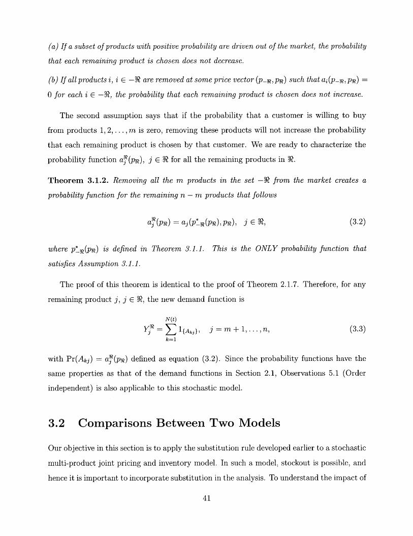
Figure 3-1: product l's demand

This figure illustrates how the system evolves. Customers arrive at a rate of A and pur-

chase one of the products or depart the system.

Before product 2 stocks out, each customer chooses product 1 with probability al(p),

product 2 with probability a2 (p) and a no-buy option with probability ao(p). After product

2 stocks out, each customer chooses product 1 with probability a (pl) and no-buy option

with probability a (pi) where ( {1}. aR(pi) and ao(pl) follow the price-dependent de-

mand substitution rule developed in Section 3.1.

-;;-;~-;::r~-r:l~i.~--sl-x-l-- rlr~----- -::: :

By contrast, the traditional approach when optimizing pricing and inventory decisions

is to assume that there is no stockout demand substitution, i.e., product 2's customers are

completely lost once the product stocks out. This implies that after product 2 stocks out,

each customer will choose product 1 with probability al (p) and a no-buy option with prob-

ability ao(p) + a2 (p).

This is the difference between the traditional pricing coordination model, referred to be-

low as the no stockout substitution model, and our model where we incorporate substitution

following our axiomatic approach. The following example shows that this difference can

affect retailer's strategy and the corresponding expected profit.

Example 3.2.1. Assume that the customer arrival rate A = 10 during a time horizon

[0,1]. Unit ordering cost for both products cl = c2 = $100. Let the demand distribution

between different products follow the attraction model with probability functions al(p) =1.5 exp-0.0

3 2pl and a(p) = 5 exp-0 0 4

p2

10-4+1.5 exp- 0 3 2pl +5 exp-

0 4p2 a2 ) 50-41.5exp

- 0 3 2p l +5 exp- 0 0 4p 2

The following table depicts the difference in the optimal strategy and expected profit

between the model with no stockout substitution and the one with the stockout substitution

rule from previous sections. These values are obtained using search algorithms.

Table 3.1: Difference on the strategy and profitInventory 1 Inventory 2 Price 1 Price 2 Ex Profit

No Stockout Substitution 7 0 $221 00 $634With Stockout Substitution 5 3 $226 $219 $700

The Table suggests that under no stockout substitution, the retailer should focus on sell-

ing only product one to achieve a maximum expected profit of $634. Because product two is

not offered, the expected profit of $634 is obtained by setting P2 to infinity and determining

the expected profit for a single product model with pi = 221. If on the other hand, the re-

tailer accepts our axiomatic approach, the retailer should order both products and increase

their total expected profit to $700.

To better understand the difference between the two models, consider the cumulative

distribution functions (CDF) of product 1's demand without, and with, stockout demand

substitution.

Two Cumulative Distribution Functions

12 14

Product 1 demand N

Figure 3-2: CDF for product 1 demand under the two models whenP2 = 219

Y2 = 3, pi = 226 and

The lower (resp. upper) curve represents the cumulative distribution function of prod-

uct 1's demand by (resp. without) taking into account stockout demand substitution. As

expected, the figure demonstrates that demand for product 1 when considering stockout

demand substitution is stochastically greater then demand for that product when stockout

substitution is not applied. This difference in demand can be significant and hence affects

retailer strategy and the corresponding expected profit.

Observe that in the previous example, in some sense, "more is better." That is, selling

two products provides a higher expected profit than offering a single product. The following

example shows that this is not always the case.

Example 3.2.2. Assume that the customer arrival rate A = 10, the time horizon is [0,1]

:;;: i ; ;_ _;;iijii; ;;_;;;-_ _;__jl__~_ _____ ___jly_~__lljllXi~liili~-I-~~;iCiii-i~ -------- __. i_-(^~_Il (l--~lii~_I-~-i~l~ii~i~Oiilij- ;iii-;~-I~I~---ii---~I^C~I~-I--__IX_-tl~

and the ordering cost for both products satisfies cl = C2 = $100. Let the demand distri-

bution between different products follow the attraction model with probability functionsa,(p) = 1.5exp-3Pl and a

2 (p) 5 exp-00 5P2

) = 510- 4 +1.5exp-0.0 3p +5exp- p2 5*10- 4 +1.5exp- 00 3P1 +5exp-00 5 p2

We first observe that for any p, A(a (p) + a 2 (p)) > Aal1(pl). This implies that the total

expected demand across the two products is greater than the expected demand of product

1 only. However, higher expected demand doesn't lead to a higher profit as is demonstrated

in the following table.

Table 3.2: More is not always better!inventory 1 inventory 2 price 1 price 2 profit

Single product 8 0 $230 00 $729

Two products 7 1 $232 $192 $717

To develop some intuition into this type of behavior, observe that when offering both

products, profit margin for product 2 is smaller than that of product 1. Removing product

2 from the portfolio increases expected demand for product 1, since al(p) < al(Pl), and this

additional demand provides a higher profit margin.

The previous example motivates a focus on situations where more products implies higher

profit. Consider similar products that differentiate only along minor characteristics such as

colors or flavors. It is often the case that retailers charge the same price for all these products.

The following proposition shows that if the probability functions that customers choose two

products are symmetric, then offering two products always produces higher expected profit

than a single product.

Before we present this proposition, we need to introduce the notion of stochastic order.

We say that the random variable X is stochastically larger than the random variable Y,

written X >st Y, if P(X > a) > P(Y > a) for all a. The following classical result is taken

from Ross [27], see his Proposition 9.1.2.

Lemma 3.2.1. X >st Y € E(f(X)) > E(f(Y)) for all increasing functions f.

Proposition 3.2.1. Assume that unit ordering costs are equal, i.e., c1 = c2 and that al(p) +

a2 (p) > max{a'(pi), a (p2)}, that is, the probability that a customer purchases when the two

products are available is no less than the probability that the customer will purchase when

only one of the two products is available. If the probability functions are symmetric, that

is, for any p, al(pi,p 2) = a 2 (P2 ,pi) and a2 (pl,p2 ) = al(p2 ,pl), then offering two products

results in an expected profit no less than when offering only one of the two products.

Proof. If the retailer sells a single product, say product 1, then there is an optimal price,

p* and optimal inventory level, y*. In this case, demand for product 1 is a poisson random

variable with mean ATal(p*). We denote this random demand as pois(ATal(p*)).

Consider a feasible pricing and inventory strategy when two products are offered. In this

policy, Pi = p2 = p* and inventory levels yl and y2 are chosen such that y1 + y2 = y~.

Let Sy,, and Sy2 be the stockout time for product 1 and product 2 respectively and

S = min{Sl, S2}, the time when stockout first happens. If S < T, then X, the total

demand cross both products satisfies X = pois(AS(al (p) + a2(p))) +pois(A(T - S)aR(p*)).

Here, we have assumed that product 2 stocks out first. But even if product 1 stocks out first,

the expression for X still holds because a(p2) = a(pi), which follows from the assumption

that the probability functions are symmetric and pl = P2 = p~.

If S > T, X = pois(AT(al(p) + a2 (p))).

It's well known that poisson random variable is stochastically increasing in its mean (see

Example 9.2(B) in Ross [27]). Therefore, it follows from the assumption al(p) + a2 (p) >

max{aR(pl), aR(p 2)} that X is stochastically larger than pois(ATaR(p*)). Lemma 3.2.1 im-

plies that E(min{X, y*}) > E(min{pois(ATaR(p*)), y*}). Hence, the profit of selling two

products, (p* - ci)E(min{X, y* }) - c1y > (p* - c1)E(min{pois(ATal (p*)), y }) - clry, the

profit of selling product 1 only. o

3.3 Summary

In this chapter, I extend the demand substitution rule to a stochastic environment. I demon-

strate the impact of our axiomatic approach to the joint pricing and inventory coordination

:;

model by incorporating the price-dependent demand substitution rule to capture customer

behavior when one of the product stocks out. The result illustrates that if the axiomatic

approach is acceptable, the optimal strategy and corresponding expected profit are quite

different than models that ignore stockout demand substitution.

48

Chapter 4

The Joint Pricing and Inventory

Game

In this chapter, I use the consumer choice theory to model retail competition among multiple

retailers. For each retailer, I develop a newsvendor model that combines inventory decisions

with a non-multiplicative price-demand model. I show that if the retailer's expected demand

is log-concave in its price, the profit is also log-concave in the price. This result implies that

in a competitive setting where multiple retailers compete on prices, a Nash equilibrium exists

in the so-called pricing game. This extends the work of Bernstein and Federgruen [8] and

Chen et al [10] from multiplicative demand models to a non-multiplicative demand model.

This part of work is done in Section 4.1.

One limitation of most pricing games models is the assumption that if one retailer stocks

out, her costumers don't switch to other retailers; they just exit the system. Therefore,

each retailer's inventory affects her own profit only, and hence retailers only compete on

price. In Section 4.2, I relax this assumption by incorporating stockout demand substitution

among retailers. This implies that if one retailer stocks out, her costumers may switch to

other retailers. Hence, each retailer's inventory level also affects other retailers' demand and

consequently their profits. Thus, retailers compete on both price and inventory, which I

refer to as the joint pricing and inventory game. I show that the quasi-concavity of each

retailer's profit function held in the pricing game doesn't have to hold in the joint pricing

and inventory game. Hence, in general there is no Nash Equilibrium in this game. However,

I characterize conditions under which a Nash equilibrium exists in the joint pricing and

inventory game.

4.1 An Extension in the Pricing Game

In this section, I assume there are n retailers in the market. Each retailer sells a similar

or identical product. Customer arrivals follow a poisson process N(t) with arrival rate

A. Without loss of generality, I assume that the time period is [0, 1]. For each customer k,

k = 1,..., N(1), denote Aki = {the event that customer k chooses retailer i} for i= 1,... n,

and Ako = {the event that customer k doesn't buy from all the n retailers }. Therefore, the

demand for retailer i is

N(1)

Yi = E {Ak i = 0, 1,..., n. (4.1)k=1

where 1{Aki is the indicator function of event Aki- I assume that different customers make

i.i.d. choices among the group of n retailers. Therefore, the probability of Aki, ai := Pr(Aki)

must be independent of k. Evidently, ai depends on the price vector p. If retailer i's

price pi increases, its probability of being chosen decreases. Therefore, ai (p) decreases in pi.

Similarly, if retailer j increases its prices the probability that a customer will chose retailer

i increases.

Given this arrival process, the demand for retailer i has a poisson distribution with

rate Aai(p). For large A, the central limit theorem implies that Y is a normal distribution

with mean 1 i(p) = Aai(p) and standard deviation ai(p) = V p) = VAai(p), i.e., Yi

pi(p) + ci V/(p), here ci is a standard normal distribution.

Denote by ci and yi the per-unit order price and order quantity, respectively, of retailer

i, i = 1,..., n. I assume that there is no salvage value, though this assumption can easily

be relaxed. While a retailer's price impacts on the profits of all retailers in a pricing game,

her order quantity affects her own profit only. The payoff function of retailer i is

wi (p, Yi) = E[pi min{yi, Y i - ciyi]. (4.2)

Under the assumption of normal distribution, the optimal inventory level, denoted y*, is

given by

y* = Pi(p) + zi a(p), (4.3)

where

zi = -1(1 - Ci, (4.4)Pi

e-z2/2and 1(z) denotes the c.d.f. of a standard normal random variable. I let 4(z) = /

2 denote

the standard normal density function. Substituting the expression for y*, in equation (4.2),

I get

pie-z/2 ()

7i (P) = (pi - ci) Pi (p) - (4.5)

where I have used the fact that for a standard normal random variable Z, E(Z - z)+ =

O(z) - z(1 - 4I(z)). I denote by 7det(p) = (pi - ci)/i(p) retailer i's profit under the price

vector p, in a deterministic system where no uncertainty prevails, i.e., demand for retailer i

equals pi(p). I also denote

pie-Z?/2fi(pi) = ci) (4.6)

which is a function that only depends on pi. I can rewrite equation (4.5) as

ji(P) = 7et(p)(1 - fi(pi)gi(p)), (4.7)

hereai(p) 1

gi(P) ai ) (4.8)

I want to show that log i (p) is strictly concave if log pi(p) is concave. First, I need the

following lemma.

Lemma 4.1.1. Let f (x) : R - R + , i = 1, 2, be twice differentiable functions. If log f (x),

i = 1, 2, are both convex functions, then fi(x) * f 2(x) is a convex function.

Proof. The convexity of log fi (x) implies that

02 log fi(zOx 2

2 fi(x)f(x) - ( X))2

S> 9~>

a2X - fi(X)

Using this inequality, I have

o2f, (x) f2(x)Ox2 Sf2(X) + fi(x) 2OX2 OX2 OX OX

(Of, ~ + f1(x)(f2f(x)) 2Of(x) of2(x)Ox fi(X) f() Ox Ox OX

"8 f (X f2 () O2 09X-

Ofi(x) Of2(x) Ofi (x) Of2 (x)21 Ox Ox +2 O 0.8@ az Ox 8x

This completes the proof.

Whitin [31] was the first to formulate the newsvendor problem with price effect. In his

model, as in ours, selling price and inventory are set simultaneously to maximize a retailer's

profit. For a review of pricing and the newsvendor problem, I refer the reader to Petruzzi

and Dada [25]. Yong [32] was the first to introduce a model that combines both additive

and multiplicative effects of price on demand. Unfortunately, his model has to satisfy some

strong assumption in order for the expected profit to be concave and lead to a tractable

model.

The following theorem states that the log-concavity of expected demand pi(p) in pi implies

strict log-concavity of profit function r(p) in pi. This condition is much simpler than the

conditions required in Yong [32].

Theorem 4.1.1. If log pi(p) is concave in pi, then log ri(p) is strictly log-concave in pi over

the region [1.01ci, 100ci].

Proof. From (4.7), we know that

(4.9)

log i (p) = log(pi - c~) + log i (p) + log(1 - f (P) gi (p)).

We first show that log fi(pi) is a convex function by showing that hi(pi) = log fi(cipi)

log Pz 2 = log pi-log 2--log(pi- 1)- 2 where z i = 4- 1(1 - ), is a convex function.

The second derivative of hi(pi) is

2w 2 2 /2

-(4 + - 4 z )ezi +pi pi

2-/ zi.eZ 2/2P 2

pi

To prove that hi(pi) is a convex function, we need to show - 0, which is equivalent

2 hi (p -1ap2gi(pi) = pt •

p

(Pi - 1)2

27 27 12-(s + Zi2 )e ipi Pi

+2-- ze -2/2 > 0.pi

We prove that this is true for pi E [1.01, 100]. Notice that the absolute value of z',

Iz| I= I-1( 1 - 1) is decreases over [1.01, 2] and increases over [2, 100]. Therefore, for any

Pi E [1.01,100],

1 1IzIl < max{L-(1 - 1 )I I-1(1 - 100} = 2.3301.

1.01 100(4.13)

/2az"(pi) -- rOp- v-- 2 implies that

( 2 r p 27rdpi

47= 3

pi

47r 223 i

pi

47 , 2 / 2 1 2

-z -2 2 ) e ipi pi

27 27r , 12 2

2 2 2 ,'2/~ e? 2 ,Pi Pi P

S(4e )e

S(4 i + 4 z11 + 4 zl,/9 -T) l":< 1.90 * 106,

+ (47 + 4- I z 2)

where the first inequality follows from pi _ 1.01 and the second inequality follows from

2 hi (ps)

ap

_ 12

pi

1

(p 1)(4.11)

(4.12)

Iz2 12z 2

(4.14)

(4.10)

(4.13). Similarly, we have

A i 2 e2/2 (2 + 22 / z 2/2 z 2 /2 ' 2 2w F Z 2/2 2 z 2/ 2e - +i + 2 i _ e /2pi P pi Pi pi p

S(22 |z) + 22 ez 2/2)z 2/2 + 2 |i e zl 2/21 Z1 2 ez 2 /2

< 1.86 *104. (4.15)

We also have

I& )a2 p I pi 1) < 2.02 * 106, (4.16)Ons (pi - 1)3 -

where the inequality follows from pi > 1.01.

(4.14), (4.15), (4.16) and Mean Value Theorem imply that for any pi, p E [1.01, 100],

Ai(Pi) - 9 <i(p ) < (1.90 • 106 + 1.86 104 + 2.02 * 106) pi Pi I < 4 * 106 pi - p 1. (4.17)

(4.17) indicates that if [pi - pl < 10-7, then |gi(pi) - gi(pi)] < 0.4. Define S = {pipi =

1.01 + 10- 7 * k, k = 0, 1, 2, ... and pi <= 100}. After calculating by computer, we find

minpEs(gi(pi)} = 0.83, which implies that mine[l.ol,loo] {gi(pi)} > 0.83 - 0.4 > 0.

This completes the proof that log fi(pi) is convex over the region [1.01ci, 100c].

From (4.8), log gy(p) = -log pl (p), which is a convex function in pi by the assumption

that log p (p) is concave. Therefore, Lemma 4.1.1 implies that fi (pj)g (p) is convex in pi and

consequently 1 - fi(pi)gi(p) is concave in pi, which implies that log(1 - fi(pi)g(p)) is concave

in pi. Given that log(pi - c) is strictly concave in pi, it follows from (4.10) that log w-j(p) is

strictly concave in pi over the region [1.01ci, 100ci]. o

Although we only show that log ri (p) is strictly log-concave in pi over the region [1.01ci,

100ci] in Theorem 4.1.1, the idea of this proof can be extended to show that log ri(p) is

strictly log-concave in pi over any region which is a subset of (ci, +oo).

The following theorem extends the pricing game model of Bernstein and Federgruen [8]

lill--- ~IXil-Li~-'--""-X~~'"~~P--~ -- I~-~.I-~ri ~lji~i~ii~i~ir~~irx~~~~nr~~~~-~ii~;~~~- :

and Chen et al [10] for multiplicative models and the work of Bernstein and Federgruen [7]

for a non-multiplicative model.

Theorem 4.1.2. If log pi (p) is concave in pi, a pure strategy Nash equilibrium exists in the

pricing game.

Proof. Theorem 4.1.1 implies that there is a unique best response function pi*(p_) for

any p-i. The continuity of p* (p_-) is implied by the continuity of 7ri(p). By Kakutani's fixed

point theorem, there must be a fixed point for best response functions p(P-i), i = 1 ... , n,

which has to be a pure strategy Nash equilibrium. O

Notice that log pi (p) is concave in pi if and only if log a (p) is concave in pi since p (p) =

Aai(p). It can be easily verified that this assumption is satisfied by the attraction models

and the linear model.

4.2 Existence of Nash Equilibrium in the Joint Pricing

and Inventory Game

In literature on pricing games, including our previous analysis, a simplified assumption is

that after a retailer stocks out, her customers exist the system, i.e., none of them switches to

other retailers. In this section, we relax this assumption. We consider two retailers, retailer

1 and retailer 2, competing in the market. Customers' arrival process is a poisson process

with arrival rate A. Before retailer 2 stocks out, each arrival customer chooses retailer 1 with

probability al(p), retailer 2 with probability a2 (p) and no-buy option with probability ao(p).

After retailer 2 stocks out, some of retailer 2's customers switch to retailer 1, and some of

them leave the system. Specifically, for each customer arriving after retailer 2 stocks out, let

ai(pi) be the probability that this customer chooses retailer 1, and aR (pj) is the probability

that the customer chooses the no-buy option. We refer readers to Lu and Simchi-Levi[16]

to see how al(p) and ao(p) are determined by following an axiomatic approach. The same

principle applies to retailer 2 if retailer 1 stocks out first. Therefore, not only the price, but

also the inventory of one retailer will affect the demand for the other retailer and consequently

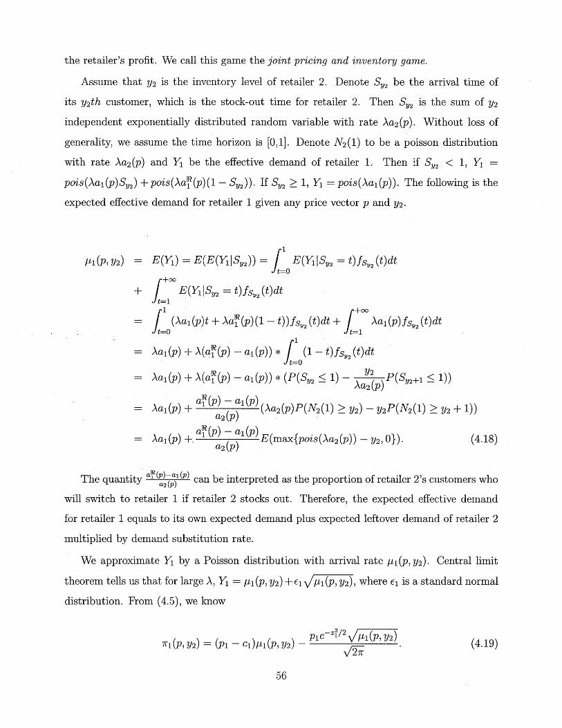
the retailer's profit. We call this game the joint pricing and inventory game.

Assume that Y2 is the inventory level of retailer 2. Denote SY2 be the arrival time of

its y2th customer, which is the stock-out time for retailer 2. Then SY2 is the sum of y2

independent exponentially distributed random variable with rate Aa2 (p). Without loss of

generality, we assume the time horizon is [0,1]. Denote N2 (1) to be a poisson distribution

with rate Aa2(p) and Y1 be the effective demand of retailer 1. Then if S, 2 < 1, Y1 -

pois(Aal(p)Sy2) +pois(Aal(p)(1 - S2)) . If SU2 1, 1 -= pois(Aal(p)). The following is the

expected effective demand for retailer 1 given any price vector p and Y2.

#1(P, Y2 ) E(Y) = E(E(Yi S 2 ))= E(YiSy2 = t)f2 (t)dt

/+oo+ j E(Y Sy2 - t)fsV (t)dt

t=1

S (Aai(p)t + Aa(p)(1- t))fsy2 (t)dt+ J Aal(p)fs 2 (t)dtt =0 =1

= ala(p) + A(a (p) - a (p)) * (1 - t)fs2(t)dt

= Aa(p) + Aa(p) - a(p)) 1 2 SAa2 (P)

Aal(p) + ) - a(p) (Aa 2 (p)P(N 2(1) > Y2) - y2P(N 2 (1) > Y2 + 1))

Aal(p)+a (p) a (p) E(maxpois(Aa2(p))- Y2, 0}). (4.18)a2 (P)

The quantity a2(p) can be interpreted as the proportion of retailer 2's customers who

will switch to retailer 1 if retailer 2 stocks out. Therefore, the expected effective demand

for retailer 1 equals to its own expected demand plus expected leftover demand of retailer 2

multiplied by demand substitution rate.

We approximate Y by a Poisson distribution with arrival rate ,i(p, Y2). Central limit

theorem tells us that for large A, Y = P (p, Y2) + E1 T 1 (, Y2), where e1 is a standard normal

distribution. From (4.5), we know

Ple-Z2/2 1 2I (p, Y2) = (P1 - C)1 1(p, Y2 ) - /2 A1(PY2) (4.19)

_L1~ _ _; _ ____~I_ __ ~__~__I_~___ ___ _____1_____1_~_^1____~l~__l_~__llll_;_i __11_. ii...ii(-;.iiii.;~-_:i-i-.i...

In the case of the pricing game, see Section 4.1, we know that if log al (p) is concave in

pi, log 71 (p) is strictly concave in pl, which implies that 7l- (p) has only one maximal point.

Unfortunately, this is not true for the joint pricing and inventory game. That is, even if

log al (p) is concave in pi, 1l (p, Y2) can have two optimal points.

150

100

50-

1 2 3 4 5 6 7 8 9 10 11

Figure 4-1: 7rx(px, 40, 6)

Example 4.2.1. We assume that cl = 1 and A = 80. Let a (p) = exp- 3 9* pP 2O.001+exp-l

3 9*P1 +exp-P2

a2(p) = __ p-_and a_(p)_ _xp-_X 3 g*1a2 0.0001-exp-l 3 9

*pl+exp-P2 and a(p) O.O01+expl .39 p For Y2 = 40 and P2 = 6, Figure

4-1 shows that 7r1 (P, 40, 6 ) can have two optimal points over pl.

To illustrate that no pure strategy Nash Equilibrium exists, fix Y2 and determine the best

response of retailer 1, pt(P2) for any given price of retailer 2, p2. Figure 2 shows that at

P2 = 6, there are two best response strategies for retailer 1, one at a higher price of $5.45,

and a second at a price of $3.59. These two price levels correspond to the two optimal points

in Figure 4-2. In addition, since the best response of retailer 1 is not monotone, we conclude

that the game is not supermodular. Thus, a pure strategy Nash equilibrium doesn't have to

exist in general for the joint pricing and inventory game. O

In the rest of this section, we characterize conditions under which a pure strategy Nash

equilibrium exists for the joint pricing and inventory game.

Figure 4-2: p*(p2)

We assume that probability functions follow the widely used attraction model ai(p) =ao+kie p+ 2 , i A 1, 2. In this case, we know from Lu and Simchi-Levi [16] that retailer

i's probability of being chosen after retailer j stocks out is a0(p) = ki-ePi 7 for i = 1, 2ao+kie

-Aipi

and j $ i.

This assumption allows to develop a new form for the expected effective demand faced

by retailer 1, Y1.

Jt=0tf 2 (t)dt +

E(YISy2 = t)fs2 (t)dt

fsY2 (t)dt)

+00= Aa'(p) - A(a'(p) - al(p)) * (P(S 2 > 1) + a2(p)

= AaR( a() (p) (Aa 2(p)P(N2 (1) < Y2 - 1) + y2P(N 2 (1) > Y2 + 1))a2(p)

- Aag(p) - (p) al(P)E(min{pois(Aa2()) Y2})a2(p)

- (A - E(min{pois(Aa2(p)), y2}))al(p), (4.20)

where the last equality follows from the fact that ()-a-( a(p)a2(p) a

P 1(p, Y2) E(Y 1 S 2 = t) fS2 (t)dt +

- (Aal(p)t + Aal(p)(1 - t))fs2 (t)dt +

ot=0 =1

= Aa(p) - A(a'(p) - al(p)) * (

~

= E(E(Y| SY2)) =

Aal (p)fsY2 (t)dt

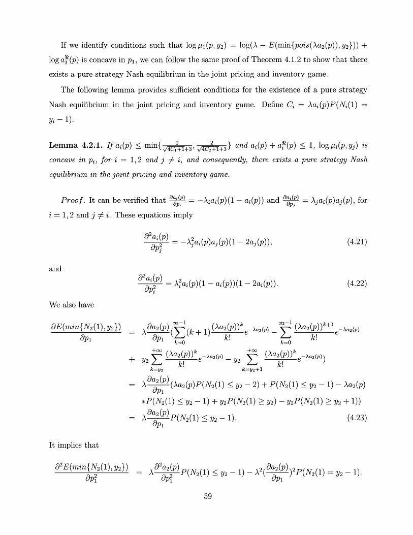
If we identify conditions such that loguI(p, Y2) = log(A - E(min{pois(Aa2(p)), Y2})) +

log a'(p) is concave in P, we can follow the same proof of Theorem 4.1.2 to show that there

exists a pure strategy Nash equilibrium in the joint pricing and inventory game.

The following lemma provides sufficient conditions for the existence of a pure strategy

Nash equilibrium in the joint pricing and inventory game. Define Ci = Aai(p)P(Ni(1) =

Yi - 1).

Lemma 4.2.1. If ai(p) < min{ +3' +3 and ai(p) + a(p) < 1, log pi(p, yj) is

, 4 C ++ 3' /4C 2 ++3

concave in pi, for i = 1, 2 and j i, and consequently, there exists a pure strategy Nash

equilibrium in the joint pricing and inventory game.

Proof. It can be verified that oai(p) = -iaia(p)(1Opi

- ai(p)) and Oa(p)Opj = Ajai(p)aj(p), for

i = 1, 2 and j - i. These equations imply

2ap

a 2ai(p) = A2ai(p)(1 - ai(p))(1 - 2ai(p)).

We also have

dE(min{N2 (1), y2 }) Oa 2 (Aa 2 (p e -a 2 (p )

- OApl (E(k + 1) k!k=O

y2- (Aa2(p) A+ ea2(p)Y k!k=O

+ 2 (Aa(2))k - Aa2(P) 2k=y

2

±00

Ek=y2 +1

(Aa 2 (p))k e-a2(P)1 -' a ()

da2 9= A (Aa2 (p)P(N 2 (1) < y2 - 2) + P(N 2(1) < Y2 - 1) - Aa 2(p)

*P(N 2(1) < y2 - 1) + y2P(N 2 (1) > y2) - y2P(N 2 (1) > y 2 + 1))

= Oa2 P(N 2(1) < Y2 - 1). (4.23)apl

It implies that

O2E(min{N 2(1), Y2 ) A2( Op-a)2P(N2 () = Y2 - 1).= 02a(P)

and

(4.21)

(4.22)

N2(1) < y2- 1)-

Therefore,

-A~a2P) P(N2 () < Y2 - 1) +A2(&~P))2P(N 2 (1) = Y2 - 1)A - E(min{N2 (1), y2 })

(A 2P)(N 2(2) 2 y~ - P))2

(A - E(min{N2 (1), y2}))2

AAa 2(p)al(p)(1 - 2al(p))P(N2 (1) < y - 1) + A2Aa 2(p) 2 al(p)2P(N 2() = Y2 - 1)A - E(mi{Nm2(1), y })

(A aa 2()a ()P(N2 (1) y -1 ))

(A - E(min{N2(1), y2})) 2

To simplify the above expression, we define.Ci = Aa(p)P(N (1) = y - 1), i=1,2, and

r = min , 4+1+1 v 2+1+} If r, i.e., ai(p) < min{ 4C +3' 1 +3} i= 1,2,

we have

Q2 log(A - E(min{N2(1), Y2}))1p2

AA a2 (p)a(1 - 2a1 (p))P(N2 (1) < 2 - 1) + 2 a2 (p)2ai(p)2P(N(1) = - 1)A - E(min{N 2(1), Y2})

(AA1 a2 (p)al(p)P(N2(1) < Y2 - 1)) 2

(A - E(min{N2(1), y 2}))2

A a 2(p)al(p)(1 - 2al(p))P(N2(1) Y2 - 1) + AA2a 2 (p)2a(p)2 (N2(1) = Y2 - 1)1 - a2 (p)

A 2a2 (p) (p) (1 - 2al(p)) + C2 Aa 2(p)al(p)2

1 - a2 (p)

(p))1 - 2a1 (p) a2(p) C2al(p) a2 (p)p 1 - a(p) 1 - a2(p) 1 - al(p)1-a 2 (p)

SAa1(p)(1 - a (p))(r + C 2 r 2) < A2al(p)(1 - al(p)), (4.24)

where the first inequality follows from the facts that E(min{N2(1),y2}) < E(N 2(1)) =

Aa 2 (p) and the last term is negative, the second inequality follows from P(N 2(1) < Y2 -1)) _

1 and definition of C2, the third inequality follows from 1-2a(p) < 1 and the assumption that1-al (p) -aj(p) < r and the last inequality follows from the definition of r. Similar inequality like

1-ai(p) -

_j_

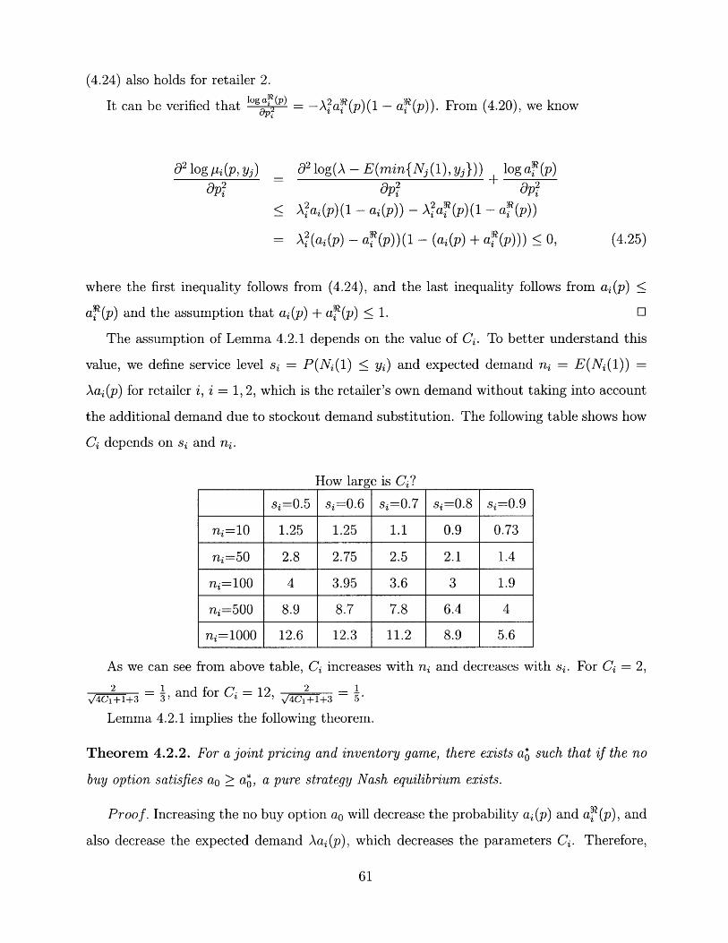
(4.24) also holds for retailer 2.

It can be verified that (P) = -A2 aF (p)(1 - a r(p)). From (4.20), we knowap 2a t/l-d Yl ~VI\fLV)V~~IV

02 log i(p, yj) 02 log(A - E(min{Nj(1), yj})) log a,(p)= +aP O- p ap

< a)(p)(I - a(p)) - Aa'(p)(1- a'(p))

= A (ai(p) - a'(p))(1 - (ai(p) + a'(p))) < 0, (4.25)

where the first inequality follows from (4.24), and the last inequality follows from a (p) <

aF (p) and the assumption that aj(p) + aF(p) < 1. O

The assumption of Lemma 4.2.1 depends on the value of Ci. To better understand this

value, we define service level si = P(Ni(1) < yi) and expected demand ni = E(N(1)) =

Aai(p) for retailer i, i = 1, 2, which is the retailer's own demand without taking into account

the additional demand due to stockout demand substitution. The following table shows how

Ci depends on si and ni.

How large is Ci?

si=0. 5 si=0.6 si=0.7 si=0.8 si=0.9

ni=10 1.25 1.25 1.1 0.9 0.73

ni=50 2.8 2.75 2.5 2.1 1.4

ni=100 4 3.95 3.6 3 1.9

ni=500 8.9 8.7 7.8 6.4 4

ni=1000 12.6 12.3 11.2 8.9 5.6

As we can see from above table, Ci increases2 = 1, and for Ci = 12, +3 1

Lemma 4.2.1 implies the following theorem.

with ni and decreases with si. For Ci = 2,

Theorem 4.2.2. For a joint pricing and inventory game, there exists a* such that if the no

buy option satisfies ao > a*, a pure strategy Nash equilibrium exists.

Proof. Increasing the no buy option ao will decrease the probability ai(p) and ai (p), and

also decrease the expected demand Aai(p), which decreases the parameters Ci. Therefore,

the conditions of Lemma 4.2.1 can be satisfied by increasing ao0 .

Now, we give some insight on the joint pricing and inventory game. Let's go back

to Example 4.2.1 to see why retailer 1 can have two optimal price points that maximize

7r(p, y2), and how the assumptions in Lemma 4.2.1 can exclude this case. Although they

lead to the same payoff, the two optimal price points represent two different strategies. The

low price point represents a strategy of competing with retailer 2 on price. The high price

point represents a strategy that pushes customer to retailer 2, and hence retailer 2 stocks

out, after which retailer 1 becomes a monopolist.

Notice the probability that a customer chooses retailer 1 after retailer 2 stocks out,

al(p,ao) = kle-P1 has the property that log a (pl, ao) has decreasing differences in

(pi, ao), i.e, if p 2 pi and a/ > ao, we have

log a' (pI, a') - log a (pl, a') < log a (p', ao) - log a'(pl, ao), (4.26)

and hence a(pa)-a(pa) > (pao)-a (p',ao) which implies that demand sensitivity fora'(pl,ao) - a (pl,ao)

retailer 1 is increasing with the no-buy option ao0.

Therefore, it is easy to understand that the high price strategy in Example 4.2.1 is based

on the fact' that the no buy option, ao = 0.0001, is relatively small such that the demand

for retailer 1 is insensitive to her price, which makes the high price strategy as profitable

as the low price strategy. Lemma 4.2.1 shows that if ai(p) and aO(p) are bounded in some

way, the high price strategy of retailer 1 has to be excluded, which makes the best response

correspondence be unique. Especially, as the no-buy option ao increases, demand becomes

more sensitive to its price. Then, the high price strategy is excluded. We can conclude

that the existence of a pure strategy Nash equilibrium in a joint pricing and inventory game

depends on the sensitivity of the retailer's demand to her price.

Lemma 4.2.1 also implies that if both retailers adopt high service level strategy, a joint

pricing and inventory game will more likely to have a pure strategy Nash Equilibrium. This

is because from the newsvendor model, we know high service level corresponds to high price

pi, which decreases ai(p) and a~f(p). At the same time, as shown in the table, C, decreases

with service level. Therefore, a high service level is more likely to imply that the assumptions

of Lemma 4.2.1 are satisfied.

4.3 Summary

In this chapter, I show the log-concavity of profit function under mild conditions. This result

and the price-dependent demand substitution rule are applied to study a retail competition

game. In this model, multiple retailers compete on price and inventory and shortage of one

product affects the demand of other products. I identify conditions under which a pure

strategy Nash equilibrium exists.

64

Chapter 5

Adaptive Safe Price

In this chapter, we use the structure developed in Almgren and Chriss [2] to model how

security's price is affected by the trader's order and its evolution over periods. This model is

also used in Huberman and Stanzl [13]. In particular, in each period, the trader's order has

temporary and permanent impact on the security's price. The initial price of the security

at time i, Pi, is observed by the trader. Given this price, the trader faces the transaction

price i = pi + Aliqi to buy the quantity qi, where Ali is a positive constant that measures

the temporary price impact of the trader's order. The new initial price for the next period

evolves according to pi+l = pi + A2iiqi + Ei, where A2i is a positive constant that measures the

permanent price impact of the trader's order and ci is a random variable. This price motion

law is illustrated in Figure 5-1.

Given this law of motion for price pi and the above analysis, the optimal policy of the

trader is given as the optimal solution of the following optimization problem:

maximize qi E{Z Eoi} (5.1)

subject to Pi = pi + Aliqi (5.2)

pi+l = pi + A2iqi + ci (5.3)

A p<p, i = 0, ... , N. (5.4)

We point out that Pi, i = 0, 1,..., N, is the trader's estimation of safety prices rather

130

125

120

115 temporary impa

110

permanent impact105-

100

Sorder is placed

0 10 20 30 40 50 60time t

Figure 5-1: The law of price motion.

than decision variables. At the beginning of each period i, the trader only has an estimate

of Pi and ,j is unknown for j > i. The formulation above is general enough to incorporate

changes in the safe price to adapt to market dynamics, which allows us to specify the order

size as a function of the safe price estimation at that period.

The objective of this chapter is to characterize the optimal trading strategy based on the

above formulation. It is easy to see that if pi > p- in period i, the trader will not purchase

anything in this period. On the other hand, it is not clear how much should the trader

purchase when pi < P. It is tempting to conclude that since the trader's goal is to maximize

the number of units of security, the trader should purchase to increase price up to pi, i.e,

purchase q = 1 . We refer to this policy as the greedy policy. Unfortunately, we show

in Section 5.1, using a counter example, that the greedy policy is not always optimal. In

Section 5.2, we show that under some reasonable conditions, the greedy policy is indeed

optimal. Remarkably, we need only impose conditions on the price impact parameters Aki,

k = 1, 2 and i = 0..., N. We do not need to make any assumption on the random variable

ci, price pi or safe price pi. In Section 5.3, we study the performance of the greedy policy

when it is not optimal. We derive a lower bound on the ratio of the value returned by the

greedy policy to the optimal value of (5.1)-(5.4). We also give a discussion on the structure

of the optimal policy in general.

5.1 Greedy Policy is Not Always Optimal

In this section, we give an example where the greedy policy is not optimal. First, we need

the following lemma.

Lemma 5.1.1. If a function f(x) is convex over [a, b], then maxxe[a,b] f(x) = max{f(a), f(b)}.

Proof. For any x E [a, b], there exists some A E [0, 1] such that x = Aa + (1 - A)b. Then,

< Af (a) + (1 - A)f (b)

< Amax{f(a), f(b)} + (1 - A)max{f(a), f(b)}

= max{f(a), f(b)}, (5.5)

which completes the proof.

This lemma tells us that the maximal value of a univariate convex function is achieved

at one of the endpoints.

For problem (5.1)-(5.4), we define Ji(pi) to be the optimal value to go from period i at

price pi. In the following example, we show that the greedy policy is not optimal.

Example 5.1.1. We set N = 1 and assume po = P, = p. Since period 1 is the last period,

it is easy to see thatP-p1

Ji (pI)0

if Pi < p,

if Pi > p.

(5.6)

J1 (pl) is a convex function over R. Therefore, for po < P,

max qo + E(O<qo < P-

S 10

J (po + \20 q0 + 60))

max{E(J(po + co)), + E(J(po + A20 1 0 Co),whereo the second equality follows from Lemma 5.1.1. Note that if Jo(

where the second equality follows from Lemma 5.1.1. Note that if Jo(po) is achieved at

Jo0(Po)

f(x) = f (Aa + (1 - A)b)

0 0.5 1 1.5 2 2.5 3 3.5 4 4.5 5

Figure 5-2: Greedy policy fails.

E(J1 (Po + co)) the trader should not order anything in period 0; otherwise he should use the

greedy policy in that period.

We define s = p- po, a = - 20 and

A = E(Jm(po + co)) - E(Jm(po + A20o -PO + 60))Alo AlO

fPP - -Po P-P A 0 - tP-o p - (t)dt --po-A20 ---- p - po - A20 - t - PO= "A (t)dt -- (t)dt

o 11 -oo A1 1 100 Al f 0- A ll ass

1s s 1 (d s= 1 ( (s - t)(t)dt - (as - t) (t)dt) - = 1 : s(t)dt - 8-, (5.7)A11 - - oo as

where 0(t) and )(t) are pdf and cdf of random variable co. The last equality follows from

integration by parts.

We set A10 = All = 0.001, A20 = 0.003, and assume that o0 follows standard normal

distribution, i.e., N(0, 1). In Figure 5-2, x-axis represents the value of s and the y-axis is A.

As we can see, A > 0 for all values of s and hence the optimal policy at period 0 is not to

order at all instead of ordering up to p. Therefore, the greedy policy is not optimal in this

example.

5.2 When is Greedy Policy Optimal?

In this section, we establish conditions under which the greedy policy is an optimal solution

to (5.1)-(5.4). For this purpose, we first show some properties of Ji(p). For notational

convenience, in this section we omit the time index of price p. The following lemma shows

a monotonicity property of Ji(p).

Lemma 5.2.1. For any i = 0, 1,..., N, Ji(p) decreases with p.

Proof. We prove the lemma by applying backward induction. For i = N, this property

easily follows from the fact that

PN-PJN (p) Al

0

if p < pN,

if p > PN

(5.8)

Assume Ji 1x(p) decreases with p. Without loss of generality, let pl - P2. We consider

three cases:

Case 1: For any pi < P2 < Pi,

max qi + E(Ji+l (pl + A2iqi + Ei))0<qi<~A-- -- , i

__ maxO<qi<Pi-p

-- li

> max<qi< Pi -P2

A )li

Ji (P2),

qi + E(J+j1 (P2 + A2iqi + Ei))

qi + E(Ji+l(P2 + A2iqi + Ci))

(5.9)

where the first inequality follows from the induction assumption and the second inequality

follows from the facts that i-pl > 1i-P2 and this is a maximization problem.

Case 2: For any P2 > Pi > pi, we have

Ji(pl) = E(Ji+l(pi + cE)) > E(Ji+l(p2 + i)) - Ji(P2 ). (5.10)

Case 3: For any pl < pi - P2, it follows from (5.9) and (5.10) that Ji(pl) > Jii()i) Ji(P2 ). O

Ji(pi) =

We now provide an upper bound on the amount lost if the starting price in period i is

increased by h, i.e., an upper bound on J(p) - Ji(p + h) for any h > 0 and i = 0,..., N.

Consider first the last period N. For any p and h > 0, we must have

(5.11)JN(p)- JN(p-+h)< +

This is easy to see by inspecting equation (5.8) for p, p + h < PN or p, p + h > PN. If p < PN

and p + h > yN, then the same equation suggests that JN(p) - JN(p + h) = PNP < 5h

because p + h > PN. The following theorem extends this observation by providing an upper

bound for any i.

Theorem 5.2.1. Define aN = and ai = max{ai+,, aja1 + (1-Aii+)} for i =

0, 1,..., N - 1. Then for any price p and h > 0, we have

Ji(p) - J (p + h) < aih, (5.12)

for any i.

Proof.

for i = N.

We prove the result using backward induction. We have shown that

Assume (5.12) holds for i + 1, for any p with p + h < pi, we know

Ji(p) max qi + E(Ji+l(p + 2iqi + Ei)) max max qi + E(Ji+(pO<qi< 5i - p O<qi <P-p-h

- li Ali

max qi + E(Ji+l(p + A2iqi + Ei))}.Pi-p- pq

- h .i P

Ali li--

(5.12) holds

+ A2iqi + Ei)),

We start by focusing on the first component of the right hand side of the above equation.

max qj + E(Ji+1 (p + A 2iqi + i)) <O<qi <i-P-h

Ali

max qi + E(Ji+l(p + h + A2iqi + Ei))}O<qi< Ji- p - h

Ali

+ai+lh = J(p + h) + ai+lh < J(p + h) + aih,

where the first inequality follows from induction assumption, the equality follows from defi-

nition of Jj(p + h), and the last inequality follows from the definition of ai.

For the second component, observe that the definition of Ji(p+h) implies that Ji(p+h) >

;I;l~__i _~ lyyl;_Lllij__:jijli_^_ii.ili~i _i;iii~_l--i;:il-~--i-:i-i---l-:Il-~--~ ~---~~Xllli CII-C--C;i___i-ii_-~iliii-i~ :-i--- i~i-~;--XII^1i---~~~l--~-~~-i -li

i-p-h + E(Ji+l(p + h + A2i pi-p-h + i)). It follows thatAli Ali

max _ qi + E(Jil1 (p + A2iqi + ;i))ji-P-h <qi< P-P

) li Ali

p - hS max {qi + E(Ji+l(p + A2iqi + i)) --fi-p-h <,qi<i-v Al i

i -p- A-h

- E(J,+(p + h + A2i h + ci))} + J(p + h).

Ali

If A2iqi h + A2i i-p-h Lemma 5.2.1 and inequality (5.13) imply thatIf Xa~i 2h + XiAli

qi + E(Ji+l(p + A 2iqi + Ei))-p-hmax (q - p ) + (p + h)

Pi-P--h <qi<PiP lili - li

h- + J(p + h) < ah + J(p + h).Ali

If A2iqi < h + A ii - p - h the induction assumption and inequality (5.13) imply thatAli

max qi + E(Ji+l(p + A2 i q i + Ei))S-p- h <qi< Pi -pAli -- li

< max {qj - pii - qi_ li

+ ai+l(h + A2 i -h _ A2iqi)} + Ji(P+ h)Ali

p -p-h= max {(1 - A2iai+l)(qi - Pi - )+ ai-p- hqi (p+h)li

+ ai+lh + Ji(P + h)

_ max{ai+, (1- A2 a+) + ai+l}h

< aih + Ji(p + h),

+ Ji(p + h)

(5.14)

where the second inequality follows from considering the two cases that 1 - A2iai+l < 0 and

1 - A2iai+l > 0.

In summary, for any p, p + h < pi, (5.12) holds.

We next consider any p with p, p + h > Pi,

Ji(P) - Ji(p + h) = E(Ji+l(p + )) - E(Ji+l(p + h + ci)) < ai+lh i aih,

max<i-- qi< Pi-P

S1i li

(5.13)

(5.15)

where the first inequality follows from induction assumption and the second inequality follows

from definition of ai.

The last possible case is p < pi and p + h > pi. We have

Ji(p) - Ji(p + h) maxO<qi

<i -p

qi + E(Ji+l(p + A2iqi + Ei)) - E(Ji+l(p + h + ci))

< max qi + E(Ji+l(p + A2iqi + Ei)) - E(Ji+l(p +0<qi<

where the last inequality follows from pi - p < h.

If A2iqi > h, Lemma 5.2.1 and inequality (5.16) imply that

Ji(p) - Ji(p + h)h

max q = < aih\1qi

If A2iqi < h, the induction assumption and inequality (5.16) imply that

J (p) - J2 (p + h) < max qi + ai+l(h - A2iqi)0<qi:

max (1 - A2iai+l)qi + ai+lhO<qi< h

-Xii

(1 - A2iai+l)< max{a i+,

where the first inequality follows from considering the two cases:

1 - A2iai+l > 0.

In summary, for any p < Pi and p + h > T, (5.12) holds.

+ ai+l}h < aih,

1 - A2iai+l : 0 and

Theorem 5.2.1 tells us that the difference between Jj(p) and Ji(p + h) is bounded by a

linear function of h with slope ai, which depends on the price impact parameters Aki but not

on the price p, noise cj, j = i,..., N - 1 and how the trader sets the safe prices pj in the

later periods j = i, . . ., N. This theorem motivates the following sufficient condition under

which the greedy policy is optimal.

Theorem 5.2.2. At period i, if the temporary and permanent price impact parameters satisfy

A2iai+l < 1,

h + ci)), (5.16)

(5.17)

(5.18)

then greedy policy is optimal to (5.1)-(5.4), i.e, if p < Pi, q - is the optimal quantity.

Proof. For any 0 < qi < q*, we have

qi + E(Ji+l(p + A2iqi + Ei)) - (q* + E(Jil(p + A2i q* + e))) qi - q + ai+lA2i (q - qi)

= (qi - qi) (1 - ai+lA2i)

< 0, (5.19)

where the first inequality follows from Theorem 5.2.1.

Thus, since Ji(p) = max0 q qi + E(Ji+1 (p + A2iqi + 60)), we have that qi = is

the optimal quantity. O

We now explain the intuition behind Theorem 5.2.2. Consider purchasing one additional

unit in period i. This unit will increase the price in period i + 1 by A2 i. Theorem 5.2.1 tells

us that starting from period i + 1, we will lose at most A2iai+l due to this price increase.

Therefore, if Eq. (5.18) is satisfied, greedy policy is optimal since what we can lose in

subsequent periods is less than what we gain in the current period.

Next we identify cases where the condition A2iai+l < 1 is satisfied, that is, we identify

cases where the greedy policy is optimal. The first case is when the temporary price impact

is greater than or equal to the permanent price impact, i.e., Ali A2i, and the permanent

price impact is nondecreasing with time, i.e., A2(i+l) < A2i. This is shown in the following

proposition.

Proposition 5.2.1. If for each i, Ali > A2i and A2i < A2(i+l), then the greedy policy is

optimal.

A 2 (N-1) <Proof. We show A2iai+l < 1 by backward induction. For i = N-l, A2(N-1)aN N A1N

A2N < 1. Assume A2iai+l < 1, then ai+l + (1-Ala+i) > ai+l. Also, ai+l + (1-=aiai+i) -

(1 - i)ai, + , hence a = (1 - i)ai+1 + -1 . Therefore, A2 (i-1)ai < A2iai

(1- li)A2iai+1 + i' < (1- L1) + A < 1. By Theorem 5.2.2, we know that the greedy

policy is optimal. O

Practical Indication : After the trader places an order for the security, he observes

an immediate price increase. If after a short time the security price begins to drop down,

then this indicates that temporary price impact is greater than permanent price impact. If,

in addition, placing the same order in the next period results in a higher permanent price

impact, and this is true for any consecutive periods, then there is a reason to believe that

the conditions of Proposition 5.2.1 are satisfied. This proposition shows that under current

market condition, the trader should greedily buy this security whenever the price falls below

his safe price. This scenario is illustrated in Figure 5-3.

140

S135

130

125

120 temporary impact i+1

115 -temporary impact permanent impact +1

110-permanent impa t i

105 -

100

rder is paced same order is placed95

0 10 20 30 40 50 60time t

Figure 5-3: First case that greedy policy is optimal.

The second case is when a unit ordered in this period will increase next period price more

than current period price, i.e., Ali < A2i, but less than buying an additional unit next period,

i.e., A2i < Al(i+1). This intuitively implies that as time progresses, the security is desirable

by more and more people.

Proposition 5.2.2. If for each i, Ali < A2i and A2i < A1(i+1), then the greedy policy is

optimal.

Proof. We show A2iai+l < 1 using backward induction. For i = N - 1, A2(N-1) aN

2(N--1) < 1. Assume A2iai+l < 1, then ai+ + (1- a+1) > a+, and ai+l - l -)A1N i -- ±i ali

I __ ~_ ___r_/l *F~__;_I_____I_ ___ ; _ _;__;_

(1 - )a+l + 1 < 1 Hence, using definition of ai, we have ai = . Therefore,

A2(i-1)ai = < 1. Theorem 5.2.2 implies that the greedy policy is optimal. EO

Practical Indication : Figure 5-4 illustrates the expected motion of prices that satisfies

the conditions of Proposition 5.2.2. After the trader places an order for the security, he

observes an immediate price increase. If he doesn't observe a price drop after a short time,

then we conclude that the temporary price impact is no more than the permanent price

impact. In addition, placing the same order in the next period results in a higher temporary

price impact than the permanent price impact, and this is true for any consecutive periods.

160 F

901 order is pced

0 10 20 30 40 50 60time t

Figure 5-4: Second case that greedy policy is optimal.

5.3 Lower Bound for Greedy Policy

In Section 5.2, we identified conditions under which the greedy policy is optimal. Unfortu-

nately, as we saw in Section 5.1, the greedy policy is not always optimal. In these cases, it

is important to identify the effectiveness of this policy.

For this purpose we start by providing insight on the structure of the optimal policy.

Evidently, the greedy policy is optimal in the last period since future prices do not matter.

temporary impact

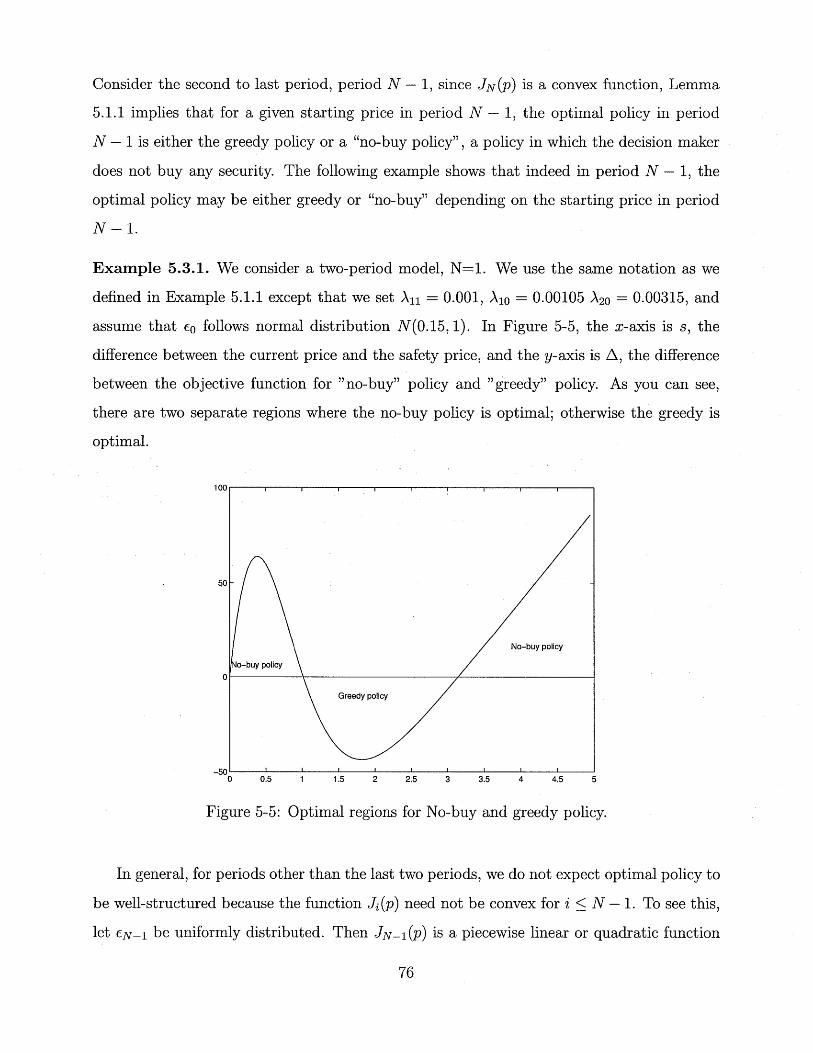
Consider the second to last period, period N - 1, since JN(p) is a convex function, Lemma

5.1.1 implies that for a given starting price in period N - 1, the optimal policy in period

N - 1 is either the greedy policy or a "no-buy policy", a policy in which the decision maker

does not buy any security. The following example shows that indeed in period N - 1, the

optimal policy may be either greedy or "no-buy" depending on the starting price in period

N- 1.

Example 5.3.1. We consider a two-period model, N=1. We use the same notation as we

defined in Example 5.1.1 except that we set An1 = 0.001, A10 = 0.00105 A20 = 0.00315, and

assume that 60 follows normal distribution N(0.15, 1). In Figure 5-5, the x-axis is s, the

difference between the current price and the safety price, and the y-axis is A, the difference

between the objective function for "no-buy" policy and "greedy" policy. As you can see,

there are two separate regions where the no-buy policy is optimal; otherwise the greedy is

optimal.

100

50-

No-buy policy

0Greedy policy

-500 0.5 1 1.5 2 2.5 3 3.5 4 4.5 5

Figure 5-5: Optimal regions for No-buy and greedy policy.

In general, for periods other than the last two periods, we do not expect optimal policy to

be well-structured because the function Ji(p) need not be convex for i < N - 1. To see this,

let EN-1 be uniformly distributed. Then JNl (p) is a piecewise linear or quadratic function

i L_... _. _ .._ ~_1..1~ i.~ -r~ll_. ~ .; - i~iil . i i. . . ... . _ii~i-C~_ i-----------. ii

that is not necessarily a convex function.

Since the structure of the optimal policy may be complex in general, it is interesting to

characterize the effectiveness of the greedy policy. For this purpose, we derive a lower bound

on the ratio of the value returned by greedy policy to the optimal value of (5.1)-(5.4).

Theorem 5.3.2. For any p, let Jo(p) be the optimal value of (5.1)-(5.4) and JJ(p) be the

value returned by greedy policy. Denote I = {i E {0, 1, ... , N - 1} A2iai+l > 1}, then

JO (p)Jo(P)

(5.20)fj 'i A2iai+liEl

Proof. For any p < )i, Let q* = '-P and = argmaxo< <Ti-,{qj + E(Jj+i(p + A2iqi +Ali _ _Xl i

ci))}. Then for any i such that A2iai+l > 1, we have

qf + E(J+,(p + A2iq + Ei))7 j + E(Ji+(p + A2i + Ei))

qf + E(Ji+l(p + A2iq + Ei))qi + E(Ji+l(p + A2iq* + Ei)) + ai+l 2i (q* -qi)

> q* + E(Ji+l(p + A2iq* + Ei)) 1> (5.21)ai+lA2i(q + E(Ji+1 (p + 2iqi + Ei))) ai+lA2i

where the first inequality follows from (5.12) and second inequality follows from the assump-

tion that A2iai+l > 1. Now we prove (5.20) by induction on the number of periods. Assume

JlP(p) > iEz\O 1a-' thenJi (p) - ie\{02iaifl

JO1 (p) = q* + E(J{(p + A20oq + co)) Sq + ( n I -)E(JI(p + A20q + co))-- 02iai+l

> ( 1+ ) (q* + E(JI(p + A20qo +60)))iGz\{O}

iEI\jOj

S( 1 o(),iel "2iai+1l

1 1A2iai+ A20 1al

+ E(JI(p + A20o 0 + )))

(5.22)

where the second inequality follows from A2iai+l > 1 and third inequality follows from (5.21).

O1

Observe that the theorem is noise-independent and price-independent, i.e., we do not

make any assumptions on the noise ci, price p and how the trader sets the safe prices Pj

in the later periods j = 1, ... , N. As we can see, the performance of the greedy policy

only depends on the temporary and permanent price impact parameters Aki, k = 1, 2 and

i = 0,1,...,N- 1.

Example 5.3.3. Consider a three-period example with A0o = 10- 5, Al = 1.2 * 10- 5, A21 =

9 * 10-6 and A02 = A12 = A22 = 10-5; these values are consistent with the examples provides

in Huberman and Stanzl [13]. Theorem 5.3.2 tells us that ) > 0.81, i.e., if a trader use

greedy policy in every period, he can get at least 81% of the maximal number of shares he

can possible get.

5.4 Summary

In- this chapter, I apply a dynamic programming approach to study optimal trading with

adaptive safe price. The analysis indicates that while the greedy is not always optimal, there

are important cases where it is. To characterize the effectiveness of greedy policy, we also

provide a lower bound on the ratio of the value returned by greedy policy to the optimal

value of (5.1)-(5.4).

Chapter 6

Conclusion and Future Research

In Chapter 2, I apply an axiomatic approach to characterize how stock-out demand substitu-

tion depends on the prices of all the products. Without any assumption on the structure of

the demand model for the remaining products, I show that there is a unique price-dependent

demand substitution rule to determine the remaining products demand model. This demand

substitution rule serves as a building block to study joint pricing and inventory coordination

as well as retail competition. Also in this chapter, I use the demand substitution rule to

study how demand sensitivity and system demand depend on the number of products.

In Chapter 3, I extend the demand substitution rule to a stochastic environment by

using consumer choices theory. I apply this result to a joint pricing and inventory coordina-

tion model, and demonstrate the impact of the substitution rule on the optimal inventory

and pricing strategy. Specifically, we compare two inventory-pricing models: one in which

demand for a product disappear during stockout time and one where substitution occurs ac-

cording to our demand substitution rule. The result illustrates that if the axiomatic approach

is acceptable, the optimal strategy and corresponding expected profit are quite different than

models that ignore stockout demand substitution. Also in this chapter, I show that more

products don't always lead retailers a higher profit and identify conditions under which two

products can provide a higher profit than a single product.

Of course Chapters 2 and 3 focus on a a single-period model, which is appropriate for per-

ishable products and fashion items. For non-perishable products, if the retailer overstocks,

inventory can be carried over to the next period. Evidently, in this case the retailer needs

to pay the inventory holding cost. If some products are out of stock, customers substitute

to other products according to the price-dependent demand substitution rule. At the same

time, the retailer needs to coordinate the price of all products. This is a multi-period joint

pricing and inventory coordination model for substitutable products, which we plan to ex-

plore in the future.

Notice that in Chapter 3, we apply an extensive search algorithm to find the optimal

price and inventory of each product so as to maximize total expected profit. To be compu-

tationally efficient, it will be interesting to characterize the optimal structure of the optimal

policy, or at least to obtain some bounds on the optimal solutions. In fact, the extensive

search algorithm is not likely to be effective as the number of products increases. One pos-

sible way to address this challenge is to apply sample path methods. Heuristic algorithms,

based perhaps on the characteristic of this optimal strategy, may also be effective. We plan

to analyze both strategies in the future.

In practice, retailers don't know the specific structure of customer demand as a function of

all product prices. Indeed, they may have only a few data points on the relationship between

price and demand, and hence this precludes the applications of inventory-pricing optimiza-

tion models. An interesting future research therefore is an empirical work that includes (i)

design of experiment; (ii) collecting data and (iii) developing a multi-product demand model

for a set of specific products. Such a model must incorporate the demand substitution rule

developed in this thesis. Otherwise, the model will be inconsistent; see Examples 2.1.1 and

2.1.2. If it's difficult to build the exact demand model, robust optimization and data-driven

optimization that takes into account stock-out demand substitution, are reasonable methods

to solve this problem.

In Chapter 4, I show that the profit function is log-concave under a mild condition. This

result generalizes the work on the newsvendor problem with price effect, and the existing

; i :;ii__(l_:iii;i__iil__l___~_~~____;_ll _ij_ _Lliilii iji:ill~-=_~--i---iii~ill-~-:ii I- ~i-~ ~ii-----j(---- -I -Iltl-il~--_illil-l---~_*_ll C-iX*;ii;_

work on pricing games. By using this result and the price-dependent demand substitution

rule developed in Chapters 2 and 3, I study the joint pricing and inventory game and ob-

tain some interesting insights on the existence of Nash equilibrium. In the future research, it

will be interesting to study the joint pricing and inventory game with more than two retailers.

In Chapter 5, I apply a dynamic programming approach to study the optimal trading

with adaptive safe price. The model assumes that a trader has a "safe price" for the secu-

rity, which is the highest price that the trader is willing to pay for this security in each time

period. The analysis indicates that while the greedy algorithm is not always optimal, there

are important cases where it is. I also provide bounds on the performance of the greedy

policy relative to the performance of the optimal policy. Future work can consider nonlinear

price impact and infinite time horizon models.

Another extension of the work in Chapter 5 is to incorporate a " a target selling price"

into the model. I define the target selling price as the price that the trader will start selling

his shares. The price region between the buying (safe) price and the target selling price

is the trader's no trade region. The trader can simultaneously buy and sell the security

with adaptive buying (safe) and selling (target) price to maximize his profit over multiple

periods. It is interesting to identify the conditions under which the multi-period arbitrage

opportunity exists if the trader has the power to affect market price by his trade.

Bibliography

[1] R.Almgren. Optimal execution with nonlinear impact functions and trading- enhancedrisk. Applied Mathematical Finance 10, 1-18. 2003.

[2] R. Almgren and N. Chriss. Optimal execution of portfolio transactions. Journal of Risk3,5-39. 2000.

[3] G. Aydin and E. L. Porteus, Joint Inventory and Pricing Decisions for an Assortment.Forthcoming in Operations Research.

[4] A. Alfonis, A. Schield and A. Schulz. Constrained portfolio liquidation in a limit orderbook model. preprint, 2007.

[5] A. Alfonis, A. Schield and A. Schulz. Optimal execution strategies in limit order bookswith general shape functions. preprint, 2007.

[6] J.R. Birge, J. Drogosz, and I. Duenyas. Setting Single-Period Optimal Capacity Lev-els and Prices for Substitutable Products. Int. J. Flexible Manufacturing Systems 10(1998), pp. 407-430.

[7] F. Bernstein and A. Federgruen. Dynamic inventory and pricing models for competingretailers. Naval Research Logistics, 51, 2, 258-274, 2004.

[8] F. Bernstein and A. Federgruen. Decentralized supply chains with competing retailersunder demand uncertainty. Management Science, 51, 1, 18-29, 2005.

[9] D. Bertsimas and A. Lo. Optimal control of execution costs. Journal of FinancialMarkets, 1, 1-50. 1998.

[10] Chen, Y. F., H. Yan, and L. Yao. Newsvendor pricing game. IEEE Transactions onSystems, Man and Cybernetics - Part A. July, 450-456, 2004.

[11] D. Gale and H. Nikaido. The Jacobian matrix and global univalence of mappings.Mathematical Annalen. 159, 81-93, 1965.

[12] R. Horn and C.Johnson. Topics in matrix analysis. Combridge University Press, 1991.

[13] G. Huberman and W. Stanzl. Optimal liquidity trading. Review of Finance 9, 165-200.2005.

[14] S. Iyengar and M. Lepper. When choice is demotivating: can one desire too much of agood thing? Journal of Personality and Social Psychology. 79. 995-1006. 2000.

[15] S. Lippman and K. Mccardle. The competitive newsboy. Operations Research. 45.54-65, 1997.

[16] Y. Lu and D. Simchi-Levi. A price-dependent demand substitution rule and its appli-cations. The MIT Operations Research Center technical report. 2008.

[17] Y. Lu and D. Simchi-Levi. The joint pricing and inventory game. The MIT OperationsResearch Center technical report. 2008.

[18] Y. Lu. Essays on inventory, pricing and financial trading policy. In preparation. MITOperations research center PhD thesis.

[19] B. Maddah and E. Bish. Joint pricing, assortment and inventory decisons for a retailer'sproduct line. Navel Research Logistics. 54. 315-330. 2007.

[20] C. C. Moallemi, B. Park and B. Van Roy. The Execution Game. preprint, 2007.

[21] S. Mahajan and G. Van Ryzin. Inventory competition under dynamic consumer choice.Operations Research. 49. 646-657, 2001.

[22] S. Netessine and N. Rudi. Centralized and competitive inventory models with demandsubstitution. Operations Research. 51. 329-335, 2003.

[23] A. Obizhaeva and J. Wang. Optimal Trading Policy and Demand/Supply Dynamics.preprint, 2006.

[24] M. Parlar. Game theoretic analysis of the substitutable product inventory problemwith random demands. Naval research logistics. 35. 397-409, 1988.

[25] N. Petruzzi and M. Dada. Pricing and newsvendor problem: a review with extensions.Operations Research, 47, 183-194, 1999.

[26] K.Rajaram and C.S.Tang. The Impact Of Product Substitution On Retail Merchan-dising. European Journal of Operational Research. 135(3): 582-601. 2001.

[27] S. Ross. Stochastic Processes. John & Sons, Inc. 1996.

[28] G. Van Ryzin and S. Mahajan. On the relatonship between inventory costs and varietybenefits in retail assortments. Management Scinece. 45. 1496-1509. 1999.

[29] S. Smith and N. Agrawal. Management of multi-item retail inventory systems withdemand substitution. Operations Research. 48. 50-64. 2000.

[30] A. Schied and T. Schneborn. Optimal Portfolio Liquidation for CARA Investors.preprint, 2007.

[31] M. Whitin. Inventory control and price theory. Managment Science, 2, 61-68, 1955.

[32] L. Yong. Price, inventory and the structure of uncertern demand. New Zealand Oper.Res. 6, 157-177, 1978.