FOUR ESSAYS IN FINANCIAL MATHEMATICS -...
206
UNIVERSITÀ DEGLI STUDI DI PADOVA DIPARTIMENTO DI MATEMATICA SCUOLA DI DOTTORATO DI RICERCA IN SCIENZE MATEMATICHE INDIRIZZO: MATEMATICA COMPUTAZIONALE CICLO XXIII FOUR ESSAYS IN FINANCIAL MATHEMATICS Direttore della Scuola: Ch.mo Prof. Paolo Dai Pra Coordinatore d’indirizzo: Ch.mo Prof. Paolo Dai Pra Supervisore: Ch.mo Prof. Wolfgang J. Runggaldier Dottorando: Claudio Fontana
-
Upload
phungduong -
Category
Documents
-
view
216 -
download
0
Transcript of FOUR ESSAYS IN FINANCIAL MATHEMATICS -...

UNIVERSITÀ DEGLI STUDI DI PADOVA
DIPARTIMENTO DI MATEMATICA
SCUOLA DI DOTTORATO DI RICERCA IN SCIENZE MATEMATICHE
INDIRIZZO: MATEMATICA COMPUTAZIONALE
CICLO XXIII
FOUR ESSAYS IN FINANCIAL MATHEMATICS
Direttore della Scuola: Ch.mo Prof. Paolo Dai Pra
Coordinatore d’indirizzo: Ch.mo Prof. Paolo Dai Pra
Supervisore: Ch.mo Prof. Wolfgang J. Runggaldier
Dottorando: Claudio Fontana


Four essays in financial mathematics:
An abstract and unifying approach to mean-variance optimization problems
Measure changes for reduced-form credit risk models
Diffusion-based models for financial markets without martingale measures
Weak no-arbitrage conditions: characterization, stability and hedging problems
Claudio Fontana
This version: August 29, 2011
Abstract
The first Chapter of the Thesis presents a general and abstract framework for the analysis ofmean-variance portfolio optimization problems. Under a minimal no-arbitrage condition, we con-sider a whole range of quadratic optimization problems, which are solved in a unified way. Wegive general and model-independent characterizations of the optimal solutions as well as abstractgeneralizations of classical results from financial economics such as two-fund separation results,mean-variance efficiency and a CAPM-type formula. Finally, we apply our general results to thevaluation of contingent claims according to several mean-variance indifference valuation rules.
The second Chapter considers a general reduced-form credit risk model, where the defaulttime is modeled as a doubly stochastic random time with default intensity driven by a diffusionaffine process. We characterize the family of all locally equivalent probability measures whichpreserve the affine structure of the model by giving necessary and sufficient conditions on theirdensity process. We illustrate the usefulness of our results first in the context of a jump-to-defaultextension of the popular Heston (1993) stochastic volatility model and then in the context of amore general hybrid equity/credit risk multifactor model, providing applications of interest in viewof risk management as well as pricing purposes.
The third Chapter deals with general diffusion-based models and shows that, even in the absenceof an Equivalent Local Martingale Measure, the financial market may still be viable, in the sensethat strong forms of arbitrage are ruled out. Relying partly on the recent literature, we providenecessary and sufficient conditions for market viability in terms of the market price of risk processand martingale deflators. Regardless of the existence of a martingale measure, we show that thefinancial market may still be complete and contingent claims can be valued under the original(real-world) probability measure, provided we use as numéraire the Growth-Optimal Portfolio.
Finally, the fourth Chapter deals with no-arbitrage conditions which are weaker than the clas-sical No Free Lunch with Vanishing Risk (NFLVR) criterion, providing necessary and sufficientconditions for their validity in terms of the characteristics of the discounted price process. Westudy the stability of weak no-arbitrage conditions with respect to changes of numéraire, absolutelycontinuous changes of the reference probability measure and restrictions/enlargements of the ref-erence filtration. In particular, we prove that weak no-arbitrage conditions, unlike the classical NoArbitrage (NA) and NFLVR criteria, are in general robust with respect to these changes. Finally, weprovide a general characterization of attainable contingent claims and market completeness withoutrelying on the NFLVR condition.
ii
Sunto
Il primo Capitolo di questa Tesi contiene un approccio generale e astratto a problemi di ottimiz-zazione di portafoglio secondo un criterio media-varianza. In particolare, vengono studiati e risolticongiuntamente diversi problemi di ottimizzazione in media-varianza, assumendo unicamente unacondizione minimale di non-arbitraggio. Le soluzioni ottime a tali problemi vengono descritte e-splicitamente, senza alcuna ipotesi sulle caratteristiche del modello sottostante. Inoltre, vengonopresentate generalizzazioni di risultati classici dell’economia finanziaria, come il teorema di sepa-razione in due fondi, la frontiera efficiente media-varianza e una formula di tipo CAPM. Infine, irisultati generali ottenuti vengono applicati alla valutazione di strumenti finanziari.
Il secondo Capitolo è dedicato allo studio di un modello generale a forma ridotta per il rischiodi credito, in cui il tempo di fallimento viene modellizzato come un tempo aleatorio doppiamentestocastico la cui intensità è funzione di un processo diffusivo di tipo affine. Si ottiene una carat-terizzazione completa della famiglia di tutte le misure di probabilità localmente equivalenti chepreservano la struttura affine del modello, formulando condizioni necessarie e sufficienti sul pro-cesso densità. L’utilità di questi risultati generali viene illustrata prima nel contesto di un modello avolatilità stocastica di Heston (1993) con l’aggiunta di un possibile fallimento e succesivamente nelcontesto di un modello multi-fattoriale più generale che consente di modellizzare congiuntamente ilrischio di credito e il rischio di mercato. Si considerano applicazioni di interesse per la valutazionedi strumenti derivati come anche per il risk management.
Il terzo Capitolo è dedicato allo studio di modelli basati su processi diffusivi. In particolare,viene mostrato che, anche in assenza di una Misura Martingala Locale Equivalente, il mercato fi-nanziario può essere privo di forme forti di arbitraggio. Basandoci in parte sulla letteratura recente,vengono fornite condizioni necessarie e sufficienti per l’assenza di forme forti di arbitraggio. Talicondizioni coinvolgono il prezzo di mercato del rischio e processi martingale deflator. Indipenden-temente dall’esistenza di una misura martingala, si dimostra che il mercato finanziario può esserecompleto e strumenti derivati possono essere valutati rispetto alla misura di probabilità del mondoreale, utilizzando come numéraire il Growth-Optimal Portfolio.
Infine, il quarto Capitolo contiene uno studio delle condizioni di non-arbitraggio più deboli delclassico criterio No Free Lunch with Vanishing Risk (NFLVR). Vengono fornite condizioni neces-sarie e sufficienti per la validità di tali condizioni deboli di non-arbitraggio, espresse rispetto allecaratteristiche del processo che rappresenta il prezzo scontato degli asset. Viene anche studiata lastabilità delle condizioni deboli di non-arbitraggio rispetto a cambiamenti di numéraire, cambia-menti assolutamente continui della misura di probabilità di riferimento e restrizioni/allargamentidella filtrazione di riferimento. In particolare, si dimostra che le condizioni deboli di non-arbitraggioconsiderate nel presente lavoro godono di buone proprietà di stabilità, al contrario di quanto accadeper le classiche condizioni di Non Arbitraggio (NA) e NFLVR. Infine, presentiamo una caratte-rizzazione generale dei titoli finanziari che possono essere replicati, dimostrando che il mercatofinanziario può essere completo anche in assenza della condizione NFLVR.
iii

iv

Contents
Introduction 1
1 An abstract and unifying approach to mean-variance optimization problems 51.1 Introduction . . . . . . . . . . . . . . . . . . . . . . . . . . . . . . . . . . . . . . 51.2 General setup and problem formulation . . . . . . . . . . . . . . . . . . . . . . . 61.3 Mathematical tools and general results . . . . . . . . . . . . . . . . . . . . . . . . 81.4 Mean-variance problems and mean-variance efficiency . . . . . . . . . . . . . . . 151.5 Mean-variance indifference valuations . . . . . . . . . . . . . . . . . . . . . . . . 211.6 Connections to the literature . . . . . . . . . . . . . . . . . . . . . . . . . . . . . 27
2 Measure changes for reduced-form affine credit risk models 312.1 Introduction . . . . . . . . . . . . . . . . . . . . . . . . . . . . . . . . . . . . . . 312.2 General setup and preliminaries . . . . . . . . . . . . . . . . . . . . . . . . . . . 342.3 The affine structure under a change of measure . . . . . . . . . . . . . . . . . . . 372.4 Application: the Heston with jump-to-default model . . . . . . . . . . . . . . . . . 49
2.4.1 Equivalent changes of measure . . . . . . . . . . . . . . . . . . . . . . . . 502.4.2 Characterization of Equivalent (Local) Martingale Measures . . . . . . . . 522.4.3 The Minimal Martingale Measure . . . . . . . . . . . . . . . . . . . . . . 56
2.5 Application: a multifactor equity/credit risk model with stochastic volatility . . . . 592.5.1 The modeling framework . . . . . . . . . . . . . . . . . . . . . . . . . . . 592.5.2 Risk management applications . . . . . . . . . . . . . . . . . . . . . . . . 662.5.3 Risk-neutral measures and valuation of default-sensitive payoffs . . . . . . 702.5.4 The incomplete information case . . . . . . . . . . . . . . . . . . . . . . . 802.5.5 Connections to the literature . . . . . . . . . . . . . . . . . . . . . . . . . 86
2.6 Conclusions and further developments . . . . . . . . . . . . . . . . . . . . . . . . 87
3 Diffusion-based models for financial markets without martingale measures 893.1 Introduction . . . . . . . . . . . . . . . . . . . . . . . . . . . . . . . . . . . . . . 893.2 The general setting . . . . . . . . . . . . . . . . . . . . . . . . . . . . . . . . . . 913.3 No-arbitrage conditions and the market price of risk . . . . . . . . . . . . . . . . . 933.4 The growth-optimal portfolio and the numéraire portfolio . . . . . . . . . . . . . . 1013.5 Replicating strategies and completeness of the financial market . . . . . . . . . . . 106
v

CONTENTS
3.6 Contingent claim valuation without ELMMs . . . . . . . . . . . . . . . . . . . . . 1093.6.1 Real-world pricing and the benchmark approach . . . . . . . . . . . . . . 1103.6.2 The upper hedging price approach . . . . . . . . . . . . . . . . . . . . . . 1113.6.3 Utility indifference valuation . . . . . . . . . . . . . . . . . . . . . . . . . 113
3.7 Conclusions, extensions and further developments . . . . . . . . . . . . . . . . . . 117
4 Weak no-arbitrage conditions: characterization, stability and hedging problems 1194.1 Introduction . . . . . . . . . . . . . . . . . . . . . . . . . . . . . . . . . . . . . . 1194.2 General setup and preliminaries . . . . . . . . . . . . . . . . . . . . . . . . . . . 1224.3 Characterization of weak no-arbitrage conditions . . . . . . . . . . . . . . . . . . 124
4.3.1 No Unbounded Increasing Profit . . . . . . . . . . . . . . . . . . . . . . . 1244.3.2 No Immediate Arbitrage Opportunity . . . . . . . . . . . . . . . . . . . . 1284.3.3 No Unbounded Profit with Bounded Risk . . . . . . . . . . . . . . . . . . 135
4.4 Stability properties of weak no-arbitrage conditions . . . . . . . . . . . . . . . . . 1444.4.1 Changes of numéraire . . . . . . . . . . . . . . . . . . . . . . . . . . . . 1444.4.2 Absolutely continuous changes of measure . . . . . . . . . . . . . . . . . 1504.4.3 Changes of the reference filtration . . . . . . . . . . . . . . . . . . . . . . 155
4.5 General characterizations of hedgeable contingent claims . . . . . . . . . . . . . . 1704.5.1 Maximal elements . . . . . . . . . . . . . . . . . . . . . . . . . . . . . . 1714.5.2 Attainable contingent claims and market completeness . . . . . . . . . . . 174
4.6 Conclusions and further developments . . . . . . . . . . . . . . . . . . . . . . . . 1814.7 Appendix . . . . . . . . . . . . . . . . . . . . . . . . . . . . . . . . . . . . . . . 182
References 187
vi
Introduction
As the title indicates, this Thesis consists of four essays dealing with some issues arising in math-ematical finance. In the first chapter, we shall start with a general and abstract perspective onmean-variance portfolio optimization problems, which represent a classical, but still active, fieldof research in financial mathematics. Then, motivated by a popular approach to the modeling ofcredit risk which has emerged in the last decade, the second chapter deals with more theoreticalquestions concerning the stability of certain structural properties of a credit risk model under achange of measure. Finally, in the third and fourth chapters, we shall deal with some foundationalissues which have recently attracted the attention of several researchers. More specifically, we shallbe concerned with the analysis of financial market models which satisfy robust no-arbitrage condi-tions, which are in particular weaker than the classical no-arbitrage criteria usually adopted in theliterature. We now present a brief description of the contents of the four chapters of the Thesis,referring to the introductory sections of each chapter for a more thorough discussion as well as formore references to the related literature.
Chapter 1, which is based on Fontana & Schweizer (2011), deals with classical mean-varianceportfolio selection problems. We choose to work in a very general and abstract setting, simi-lar to that originally introduced in Schweizer (1997),(2001a), which allows us to obtain model-independent results under the minimal no-arbitrage condition of no approximate riskless profits inL2. By relying on projection techniques in Hilbert spaces, we provide general characterizations ofthe solutions to abstract versions of the classical Markowitz portfolio selection problems as well asof mean-variance hedging and utility maximization problems. In particular, our abstract frameworkallows to treat different mean-variance problems in a unified manner, showing in a clear way howthe corresponding optimal solutions are related. Generalizing the classical two-fund-separation the-orem, we show that the optimal solutions to all mean-variance problems can be decomposed intothe sum of a fixed minimum variance element and a multiple of an additional fixed element givenby the best L2-approximation of the riskless payoff 1 onto the set of all cumulated (undiscounted)gains from trade. Furthermore, only the amount invested into the latter depends on the specificproblem under consideration. We also derive abstract generalizations of classical results from fi-nancial economics such as a characterization of the mean-variance efficient frontier, a CAPM-typeformula and a general solution to the problem of maximizing the Sharpe ratio. Finally, we alsoconsider the problem of valuing square-integrable contingent claims according to several mean-variance indifference valuation rules, for which our abstract mean-variance theory yields generaldescriptions of the corresponding indifference values, thus extending some results of Mercurio
1

Introduction
(2001), Møller (2001), Schweizer (2001a) and Sun & Wang (2005),(2006). In particular, underthe simplifying assumption that a zero-coupon bond can be (approximately) attained in the abstractfinancial market, all mean-variance indifference valuation formulae admit a very natural economicinterpretation. Related results can also be found in Chapter 1 of Fontana (2010b).
Chapter 2 starts by considering a general reduced-form credit risk model, where the defaulttime is modeled as a doubly stochastic random time with default intensity driven by an affine dif-fusion process. In the first part of the Chapter, we characterize the family of all locally equivalentprobability measures which preserve the affine structure of the model by giving necessary and suf-ficient conditions on their density process. In particular, this allows for a rigorous treatment ofdiffusive and jump-type risk premia and shows that the affine structure is preserved under rathergeneral risk-premia specifications, which nest most of the specifications usually adopted in the lit-erature. As an application, we consider a jump-to-default extension of the popular Heston (1993)stochastic volatility model, giving a complete description of the family of all risk-neutral measureswhich preserve the structure of the model, thus extending and sharpening the results of Wong &Heyde (2006). Always in the context of the Heston with jump-to-default model, our general resultsallow us to easily answer the question of whether discounted asset prices are true martingales oronly local martingales under a given risk-neutral measure and the question of whether the so-calledMinimal Martingale Measure exists. Finally, we illustrate the usefulness of our results on affine-preserving measure changes in the context of a hybrid equity/credit risk model, as considered inseveral recent papers (see e.g. Carr & Linetsky (2006), Campi et al. (2009), Carr & Wu (2010)and Cheridito & Wugalter (2011)). We propose a class of multifactor models, allowing for bothstochastic volatility and stochastic default intensity. In particular, we ensure that the affine struc-ture of the model is preserved under both the physical and the risk-neutral probability measure thusenabling us to explicitly compute several key quantities of interest for risk management as well aspricing applications. Finally, we shall also briefly consider the incomplete information case, wheresome components of the underlying driving process are not perfectly observable to market partici-pants. As in Fontana (2010a) and Fontana & Runggaldier (2010), this will lead to the formulationof a suitable filtering problem.
In Chapter 3, which is based on Fontana & Runggaldier (2011), we consider a general classof diffusion-based models and show that, even in the absence of an Equivalent Local MartingaleMeasure (ELMM), the financial market may still be viable, in the sense that strong forms of arbi-trage are excluded and portfolio optimization problems can be meaningfully solved. Relying partlyon the recent literature (see e.g. Karatzas & Kardaras (2007), Hulley & Schweizer (2010) and Kar-daras (2010a)), we provide necessary and sufficient conditions for market viability in terms of themarket price of risk process and the existence of a martingale deflator. In particular, a martingaledeflator can be considered as a weaker counterpart to the density process of a traditional ELMMand inherits most, but not all, of the useful properties of the latter. We then explicitly computethe growth-optimal portfolio (GOP), which is also shown to possess the numéraire property and tocoincide with the reciprocal of a martingale deflator. Regardless of the existence of a well-definedELMM, we show that the financial market may still be complete and contingent claims can be val-ued under the original (real-world) probability measure. In particular, we discuss three different
2
Introduction
but related valuation approaches: real-world pricing, upper-hedging pricing and utility indifferencepricing. In the special case of a complete financial market, we show that these three valuation rulesyield the same valuation formula, which amounts to taking the expectation (under the real-worldprobability measure) of the GOP-discounted payoff. We also discuss relations with Stochastic Port-folio Theory and with the Benchmark Approach, where financial market models not admitting anELMM are typically encountered, see e.g. Fernholz & Karatzas (2009), Platen (2006),(2009) andPlaten & Heath (2006).
Chapter 4 is concerned with the analysis of no-arbitrage conditions which are weaker than theclassical No Arbitrage (NA) and No Free Lunch with Vanishing Risk (NFLVR) conditions consideredin the seminal work of Delbaen & Schachermayer (1994). More specifically, we shall analyze theNo Unbounded Increasing Profit (NUIP), the No Immediate Arbitrage Opportunity (NIAO) andthe No Unbounded Profit with Bounded Risk (NUPBR) conditions. We provide necessary andsufficient conditions for the validity of NUIP/NIAO/NUPBR in terms of the characteristics of thediscounted price process of the risky assets. In particular, this allows us to generalize the resultsof Chapter 3 to more general financial market models based on continuous semimartingales. Wethen study the stability properties of the NUIP/NIAO/NUPBR no-arbitrage conditions with respectto several modifications of the structure of the underlying financial market model. More precisely,we analyze the impact of changes of numéraire, of absolutely continuous changes of the referenceprobability measure and of restrictions/enlargements of the reference filtration. The main messageis that the weak NUIP/NIAO/NUPBR no-arbitrage conditions possess stronger stability propertiesthan the classical NA and NFLVR criteria, thus confirming the economic soundness of the weak no-arbitrage conditions considered in the present work. Finally, assuming that the NUPBR conditionholds, we provide an abstract and general characterization of attainable contingent claims, withoutrelying on the full strength of the classical NFLVR condition. In particular, we obtain naturalgeneralizations of the classical results of Ansel & Stricker (1994) and Delbaen & Schachermayer(1995c) on the attainability of contingent claims, with martingale deflators replacing the traditionalELMMs. Finally, we generalize the second fundamental theorem of asset pricing to the situationwhere the NFLVR condition fails to hold.
3


Chapter 1
An abstract and unifying approach tomean-variance optimization problems
1.1 Introduction
Mean-variance portfolio optimisation is one of the classical problems in financial economics. Manypapers have been written on the subject, and many different settings and versions have been studied.So what is there left to be said?
We offer in this paper a new perspective that allows to treat mean-variance portfolio problemsin a simple and yet general way. Our approach does not depend on any particular model and usesonly simple mathematics. The key for this is a change of parametrisation.
Consider one standard formulation of the classical Markowitz problem (there are other versionsand we discuss them all in the paper): Given a financial market, find a portfolio with maximal return(mean) given a constraint on its risk (variance). The familiar mathematical description is to searchfor a (self-financing) strategy ϑ whose resulting gains from trade GT (ϑ) maximise E[GT (ϑ)] overall allowed ϑ ∈ Θ subject to Var[GT (ϑ)] ≤ σ2 for some constant σ2 > 0. The control variableis the strategy ϑ. In a one-period model with returns given by an Rd-valued random variable ∆S,a strategy is simply a constant vector ϑ ∈ Rd, and trading gains are the scalar product ϑ>∆S. Ina continuous-time model with asset prices described by an Rd-valued semimartingale (St)0≤t≤T ,a strategy is an Rd-valued predictable S-integrable process (satisfying some technical conditions),and GT (ϑ) is given by the real-valued stochastic integral
∫ T0ϑu dSu.
The very simple idea of our approach is that we need not look at S and ϑ separately — all thatmatters for our problem isGT (ϑ). Since this depends linearly on ϑ, the set of all possible gains fromtrade in a frictionless financial market is simply a linear space. (Of course, frictions or transactioncosts will complicate this; but then we already leave the classical setting.) Moreover, that space Gof gains from trade g should be a subset of L2(P ) since our problem formulation involves meanand variance. In other words, we no longer look at trading strategies as control variables, but onlyat the resulting final positions. It turns out that this change of parametrisation from Θ to G makeseverything very simple and tractable.
5

Chapter 1. An abstract and unifying approach to mean-variance optimization problems
Of course, this idea is not completely new. It has been used (and, to the best of our knowledge,introduced) in Schweizer (1997) and has been picked up by other authors more recently. We givea detailed discussion of related literature in Section 1.6. However, the systematic exploitationfor a whole range of four mean-variance optimisation criteria seems to be missing so far. Weexplicitly work out the connections between the four solutions, and we do all this carefully inan undiscounted framework. Our results include explicit formulas, two-fund separation results, aCAPM-type relation, and explicit indifference valuation rules.
The paper is structured as follows. Section 1.2 presents the general setup and the formulation ofour four mean-variance optimisation problems. Section 1.3 contains the mathematics — it solvesthe four problems explicitly and provides a number of connections between their solutions. Weeven do this more generally than discussed above, by replacing g with g − Y for some exogenousextra financial position. Section 1.4 starts on the financial economics; it determines the mean-variance efficient frontier, presents a CAPM-type relation, and derives two different but relatedtwo-fund separation results. Section 1.5 introduces mean-variance indifference valuation. Becausewe can compute the values of our optimisation problems explicitly, we can also explicitly obtain,for a suitable chosen Y , the value (financial amount) h at which an agent is indifferent, under amean-variance criterion and at optimal investment, between either selling a contingent claim H fora compensation of h or not selling H and not getting extra money. Finally, Section 1.6 contains adetailed discussion of related work in the literature.
1.2 General setup and problem formulation
This section describes the abstract financial framework and introduces the main mean-varianceportfolio optimisation problems we are interested in. For a given probability space (Ω,F , P ),denote by L2 := L2(Ω,F , P ) the space of all real-valued square-integrable random variables withthe usual scalar product (X, Y ) = E[XY ] and norm ‖X‖L2 = (E[X2])1/2. Let G be a givennonempty subset of L2, denote by G⊥ := X ∈ L2 | (X, Y ) = 0 for all Y ∈ G its orthogonalcomplement in L2, and write G for its closure in L2. Finally, let B be a real-valued random variablein L2 such that B > 0 P -a.s.
The financial interpretation is as follows. Think of a time horizon T ∈ (0,∞) and let t = 0 bethe initial time. Then G represents the set of all undiscounted cumulated gains from trade (evaluatedat time T ) generated by suitable self-financing trading strategies starting at t = 0 from zero initialcapital. The element B represents the strictly positive value (at the final time T ) of a numéraireasset and can, but need not, be interpreted as the final value of a savings account. We avoid callingB a “riskless” asset; in fact, investing one unit of money in this asset only guarantees that we endup at T with the strictly positive amount B, which is however random and can be strictly less thanthe initial investment of 1. The set cB+g | c ∈ R, g ∈ G = RB+G then represents the set of allattainable undiscounted final wealths, i.e. all those square-integrable payoffs or contingent claimswhich can be replicated in the abstract financial market (B,G) by following a self-financing strategystarting from some initial capital c. Note that we do not assume that G is closed in L2. Square-
6

1.2 General setup and problem formulation
integrability is imposed to ensure existence of means and variances, which is a basic necessaryassumption when dealing with mean-variance problems. Finally, the Hilbert space structure of L2
allows an easy and efficient derivation of general solutions to several mean-variance problems, aswill be shown in Section 1.3.
Remark 1.2.1. It is worth emphasising that apart from the obvious requirement of square-integra-bility, the present setup for an abstract financial market does not rely on any underlying modellingstructure. As a consequence, all the results we are going to present are model-independent, and inparticular hold for both discrete- and continuous-time models. We refer the reader to Examples 1–3in Schweizer (1999) for an illustration of how typical financial models can be embedded into thepresent abstract setting.
Let us now introduce a basic standing assumption for the rest of the paper.
Assumption I. The two following conditions hold:
(a) G is a linear subspace of L2.
(b) There are no approximate riskless profits in L2, meaning that G does not contain 1.
Intuitively, part (a) of Assumption I amounts to considering a frictionless financial market with-out constraints or other restrictions on trading. The condition 1 /∈ G of no approximate risklessprofits in L2 in part (b) represents an abstract and minimal no-arbitrage condition. It can be equiv-alently formulated as R ∩ G = 0, and this amounts to excluding the undesirable situation wherean agent is able to reach, or approximate in the L2-sense, a deterministic riskless final wealth fromzero initial capital. As will be shown in the next section, the condition of no approximate risklessprofits in L2 is necessary and sufficient for the solvability of the quadratic problems we are nowgoing to introduce.
In the present paper, we shall be mainly concerned with four major mean-variance portfo-lio optimisation problems, denoted as Problems (A)–(D) and formulated in the following ab-stract terms. We let Y ∈ L2 represent the final undiscounted value of a generic financial posi-tion/liability, α ∈ (0,∞) a given risk-aversion coefficient, µ ∈ R a target minimal expected valueand σ2 ∈ (0,∞) a target maximal variance. Then we consider
Problem (A’) E[g − Y ]− αVar[g − Y ] = maxg∈G
!
Problem (B’) Var[g − Y ] = min! over all g ∈ G such that E[g − Y ] ≥ µ.
Problem (C’) E[g − Y ] = max! over all g ∈ G such that Var[g − Y ] ≤ σ2.
Problem (D’) ‖Y − g‖L2 = ming∈G
!
We shall argue below that each Problem (X’) has the same optimal value as the corresponding
Problem (X) where we optimise over G instead of G.
7

Chapter 1. An abstract and unifying approach to mean-variance optimization problems
The financial interpretations of Problems (A’)–(D’) are rather obvious. In fact, (A’) describesthe portfolio optimisation problem faced by an agent with mean-variance preferences and risk-aversion coefficient α. (B’) and (C’) are abstract versions of the classical Markowitz portfolioselection problems, slightly extended by including the random liability Y . More specifically, in(B’), the agent is interested in minimising the variance of her/his final net position, given a minimaltarget level µ for its expected value. Symmetrically, in (C’), the agent wants to maximise theexpected value of her/his final net position, given a maximal target level σ2 for its variance. Finally,(D’) consists of finding the optimal quadratic hedge for Y . As we illustrate at the end of Section1.4, different investment situations can be represented via suitable choices of Y .
Remark 1.2.2. Part (b) of Assumption I excludes the case 1 ∈ G, but not the case 1 ∈ G⊥.However, the latter situation is neither particularly interesting from a mathematical point of viewnor particularly realistic from an economic point of view. In fact, 1 ∈ G⊥ mathematically meansthatE[g] = (g, 1) = 0 for all g ∈ G. But then there is nothing to optimise in (C’), and the constraintin (B’) is trivially always or never satisfied, depending on whether E[Y ] ≤ −µ or E[Y ] > −µ.Finally, (A)’ reduces to the simpler problem of minimising the variance. In financial terms, the case1 ∈ G⊥ corresponds to the situation where all undiscounted cumulated gains have zero expectationunder the original (real-world) probability measure P . In this case, there is no proper notion ofa trade-off between risk (variance) and return (expected value), and so we cannot meaningfullyconsider mean-variance portfolio optimisation problems.
Due to Remark 1.2.2, there is no loss of generality in introducing the following additionalstanding assumption for the sequel.
Assumption II. 1 /∈ G⊥, or equivalently g ∈ G | E[g] 6= 0 6= ∅.
1.3 Mathematical tools and general results
This section contains the mathematical ingredients for solving Problems (A)–(D). The Hilbert spacestructure of our framework makes the results both general and easy to obtain. We postpone to latersections all pertinent economic considerations and applications to financial problems.
Recall that the orthogonal complement G⊥ is a closed linear subspace of L2, and denote by πthe orthogonal projection in L2 on G⊥. Since G is a linear subspace of L2 by part (a) of AssumptionI, we have (G⊥)⊥ = G. This yields the direct sum decomposition L2 = G ⊕ G⊥, meaning that anyY ∈ L2 can be uniquely decomposed as
Y = gY +NY = gY + π(Y ) with gY ∈ G and NY = π(Y ) ∈ G⊥. (1.1)
Using this basic orthogonal decomposition, we can already tackle Problem (D’). Note first that
infg∈G‖Y − g‖L2 = inf
g∈G‖Y − g‖L2 . (1.2)
In fact, “≥” is clear from G ⊆ G, and conversely, any g ∈ G admits a sequence (gn)n∈N ⊆ Gconverging in L2 to g. So
infg∈G‖Y − g‖L2 ≤ ‖Y − gn‖L2 −→ ‖Y − g‖L2 as n→∞,
8

1.3 Mathematical tools and general results
and as g ∈ G is arbitrary, we also get “≤” in (1.2). In other words, the optimal value of Problem(D’) does not change if we replace G by its closure G in L2. The projection theorem then gives
infg∈G‖Y − g‖L2 = inf
g∈G‖Y − g‖L2 = min
g∈G‖Y − g‖L2 = ‖Y − gY ‖L2 = ‖NY ‖L2 . (1.3)
Optimising over the closed subspace G ensures existence and uniqueness for the solution to Problem(D), where G replaces G in (D’), and the solution is the projection in L2 of Y on G,
gY = argming∈G
‖Y − g‖L2 . (1.4)
Remark 1.3.1. Also for Problems (A’)–(C’), the optimal values do not depend on whether weoptimise over G or G. This is easily checked by the same arguments as for (1.2), using that gn → g
in L2 implies E[gn − Y ]→ E[g − Y ] and Var[gn − Y ]→ Var[g − Y ], for any Y ∈ L2.
In view of Remark 1.3.1, we henceforth consider the Problems (A)–(D) instead of (A’)–(D’),where the optimisation now goes over the closed linear subspace G instead of G. As a preliminaryto the derivation of the solutions to Problems (A)–(C), let us introduce the following variance-minimisation problem.
Problem (MV) Var[Y − g] = ming∈G
!
The solution to Problem (MV) is given in the following result and denoted by gYmv, where thesubscript “mv” stands for “minimum variance”. It is obtained by relying on the solution to Problem(D) we have just derived in (1.4).
Proposition 1.3.2. For Y ∈ L2, Problem (MV) admits in G the unique solution
gYmv := argming∈G
Var[Y − g] = gY − a∗Y(1− π(1)
), where a∗Y :=
E[NY ]
E[π(1)]. (1.5)
Proof. The key idea allowing us to reduce Problem (MV) to Problem (D) is the simple fact that
Var[Y − g] = mina∈R
E[(Y − g − a)2].
Hence we can write
ming∈G
Var[Y − g] = ming∈G
mina∈R
E[(Y − a− g)2] = mina∈R
ming∈G
E[(Y − a− g)2].
The inner minimisation over G corresponds to Problem (D) for Y − a and is solved by gY−a. Bylinearity of the projection and (1.1), we have gY−a = gY − ag1 = gY − a(1− π(1)) and so
ming∈G
Var[Y − g] = mina∈R
E[(Y − a− gY−a)2] = mina∈R
E[(NY − aπ(1)
)2]. (1.6)
9

Chapter 1. An abstract and unifying approach to mean-variance optimization problems
Now observe that because 1− π(1) is in G, we have (NY , 1− π(1)) = 0 and (π(1), 1− π(1)) = 0.This gives E[NY π(1)] = E[NY ] and E[π(1)] = E[(π(1))2] = ‖π(1)‖2
L2 > 0 since 1 /∈ G by part(b) of Assumption I. Squaring out and completing the square therefore yields
E[(NY − aπ(1)
)2]= E[π(1)]
(a− E[NY ]
E[π(1)]
)2
− (E[NY ])2
E[π(1)]+ E[(NY )2]. (1.7)
So the optimal a ∈ R is uniquely given by
a∗Y := argmina∈R
E[(NY − aπ(1)
)2]=
E[NY ]
E[π(1)],
and we obtain
gYmv := argming∈G
Var[Y − g] = gY−a∗Y = gY − a∗Y
(1− π(1)
).
The uniqueness of the solution gYmv ∈ G follows from the projection theorem via the uniqueness ofgY−a ∈ G for all a ∈ R.
Let us now introduce the notation RYmv := gYmv − Y , where “R” stands for the final “result” of
an abstract financial position. Then, for any g ∈ G, we can write
g − Y = RYmv + g − gYmv
and henceE[g − Y ] = E[RY
mv] + E[g − gYmv]. (1.8)
Furthermore, due to the optimality of gYmv ∈ G and the linearity of G, the first order condition for(MV) gives for the element RY
mv the fundamental zero-covariance property
Cov(RYmv, g) = 0 for all g ∈ G. (1.9)
Since g − gYmv ∈ G for any g ∈ G, this implies that we have
Var[g − Y ] = Var[RYmv + g − gYmv] = Var[RY
mv] + Var[g − gYmv]. (1.10)
Equations (1.8) and (1.10) show that in Problems (A)–(C), we can isolate the part coming from theminimum variance element RY
mv. Furthermore, since gYmv ∈ G and G is a linear space, the mappingg 7→ g′ := g − gYmv is a bijection of G to itself. These observations suggest that we can reduce thegeneral versions of our abstract mean-variance problems to the particular case Y ≡ 0. This will beexploited in the proofs of the three following propositions.
Remark 1.3.3. For future use in later sections, we compute the mean and variance of the optimalposition RY
mv = gYmv − Y = −NY − a∗Y (1− π(1)). From the expression for a∗Y in (1.5), we get
E[RYmv] = − E[NY ]
E[π(1)], (1.11)
and using (1.6) and (1.7) yields
Var[RYmv] = E
[(NY )2
]− (E[NY ])2
E[π(1)]. (1.12)
10
1.3 Mathematical tools and general results
We start with the solution to Problem (A), denoted by gYopt,A(γ), where γ := 1α
is the risk-tolerance coefficient corresponding to the risk-aversion coefficient α. We shall comment on thecase γ = 0 below.
Proposition 1.3.4. For Y ∈ L2 and γ ∈ [0,∞), Problem (A) has a unique solution gYopt,A(γ) ∈ G.It is explicitly given by
gYopt,A(γ) = argming∈G
Var[g − Y ]− γE[g − Y ] = gYmv + g0opt,A(γ), (1.13)
where g0opt,A(γ) ∈ G is the solution to Problem (A) for Y ≡ 0, explicitly given by
g0opt,A(γ) = argmin
g∈GVar[g]− γE[g] =
γ
2
1
E[π(1)]
(1− π(1)
). (1.14)
Proof. Notice first that with γ = 1α
, Problem (A) can be equivalently formulated as
Var[g − Y ]− γE[g − Y ] = ming∈G
!
Moreover, equations (1.8) and (1.10) allow us to write, for any g ∈ G,
Var[g − Y ]− γE[g − Y ] = Var[RYmv]− γE[RY
mv] + Var[g − gYmv]− γE[g − gYmv].
Since G is linear and contains gYmv, Problem (A) can thus be reduced to the basic problem
Var[g]− γE[g] = ming∈G
! (1.15)
More precisely, if g0opt,A(γ) ∈ G denotes the solution to (1.15), then the solution gYopt,A(γ) ∈ G to
Problem (A) in its original formulation is given by (1.13). Hence it only remains to solve (1.15).Following the same idea as in the proof of Proposition 1.3.2, we write
Var[g]− γE[g] = mina∈R
E[(g − a)2]− γE[g] = mina∈R
(E[(g − (a+ γ
2))2]− γ2
4− aγ
). (1.16)
But for Y ≡ a+ γ2, the solution of Problem (D) is by (1.4) and linearity of the projection
ga+ γ2 = (a+ γ
2)g1 = (a+ γ
2)(1− π(1)
). (1.17)
Combining this with (1.16) and completing the square gives
ming∈GVar[g]− γE[g] = min
a∈R
ming∈G
E[(g − (a+ γ
2))2]− γ2
4− aγ
= min
a∈R
E[(
(a+ γ2)π(1)
)2]− γ2
4− aγ
= min
a∈RE[π(1)]
(a− γ
21−E[π(1)]E[π(1)]
)2
− γ2
4E[1−π(1)]E[π(1)]
. (1.18)
11

Chapter 1. An abstract and unifying approach to mean-variance optimization problems
Note that as in the proof of Proposition 1.3.2, Assumption I gives E[π(1)] > 0. The last expressionin (1.18) is clearly minimised by the unique value
a∗γ :=γ
2
E[1− π(1)]
E[π(1)],
and together with (1.17), this yields
g0opt,A(γ) = argmin
g∈GVar[g]− γE[g] = ga
∗γ+ γ
2 =γ
2
1
E[π(1)]
(1− π(1)
).
The uniqueness of the solution again follows from the projection theorem via the uniqueness ofga+ γ
2 ∈ G for all a ∈ R and γ ∈ [0,∞).
Remark 1.3.5.
1. The proofs of Propositions 1.3.2 and 1.3.4 both rely on the elementary identity Var[X] =
mina∈RE[(X − a)2] for X ∈ L2. This allows us to reduce variance-minimisation problemsto particular cases of Problem (D).
2. The above trick of expressing the variance as an optimal value for a minimisation problemover R is also at the root of the appearance of the quantity 1−π(1); in fact, this is simply theprojection in L2 of the constant 1 ∈ R on G.
3. It is interesting to notice that the solution to Problem (MV) can be recovered from the solutionto Problem (A). In fact, by letting γ = 0, Proposition 1.3.4 implies that
gYopt,A(0) = argming∈G
Var[g − Y ] = gYmv.
This simple relation is in line with intuition, because γ = 0 corresponds to infinite risk-aversion (α =∞), which means in (A) that one is only interested in minimising the risk.
4. As seen in the proof of Proposition 1.3.4, the condition 1 /∈ G of no approximate risklessprofits in L2 is sufficient for ensuring the existence of a unique solution to Problem (A). Butthis condition is also necessary for the solvability of (A). In fact, suppose to the contrary thatg ∈ G solves Problem (A), but 1 ∈ G. Then g′ := g+1 ∈ G satisfies Var[g′−Y ] = Var[g−Y ]
and E[g′ − Y ] = 1 + E[g − Y ] > E[g − Y ], contradicting the optimality of g.
5. One can prove the uniqueness of the solution to (A) directly by using only its optimality. Butthe argument above via the projection theorem leads to a more compact proof.
The results obtained so far do not rely on Assumption II that 1 6∈ G⊥. It is easy to see fromProposition 1.3.4 that in the case 1 ∈ G⊥, the solutions to Problem (MV) and Problem (A) coincide,since 1 ∈ G⊥ implies π(1) ≡ 1. But for tackling Problems (B) and (C), we shall exploit AssumptionII. The basic idea is well known; it is folklore that the solutions to (B) and (C) are obtained bychoosing for the risk-aversion α in (A) a particular value, depending on the respective constraint in
12

1.3 Mathematical tools and general results
(B) or (C). In more detail, this goes as follows. In analogy to RYmv = gYmv − Y , we first introduce
the notation
RYopt,A(γ) := gYopt,A(γ)− Y = RY
mv + g0opt,A(γ) = RY
mv +γ
2
1
E[π(1)]
(1− π(1)
).
Using
Var[1− π(1)] = Var[π(1)] = E[(π(1)
)2]− (E[π(1)])2 = E[π(1)](1− E[π(1)]) (1.19)
and recalling from (1.9) the zero-covariance property of RYmv, we then obtain
E[RY
opt,A(γ)]
= E[RYmv] +
γ
2
E[1− π(1)]
E[π(1)], (1.20)
Var[RY
opt,A(γ)]
= Var[RYmv] +
γ2
4
E[1− π(1)]
E[π(1)]. (1.21)
So for 1 ∈ G⊥, we obtain E[RYopt,A(γ)] = E[RY
mv] and Var[RYopt,A(γ)] = Var[RY
mv] for allγ ∈ [0,∞). But if Assumption II holds, then we have E[1 − π(1)] = ‖1 − π(1)‖2
L2 > 0, andtherefore the functions γ 7→ E[RY
opt,A(γ)] from [0,∞) to [E[RYmv],∞) and γ 7→ Var[RY
opt,A(γ)]
from [0,∞) to [Var[RYmv],∞) are both surjective. This implies that for any µ ∈ [E[RY
mv],∞), thereexists γµ ∈ [0,∞) such that E[RY
opt,A(γµ)] = µ, and analogously, any σ2 ∈ [Var[RYmv],∞) admits
some γσ2 ∈ [0,∞) such that Var[RYopt,A(γσ2)] = σ2. Under the (standing) Assumptions I and II,
this simple observation allows us to derive the solutions to Problems (B) and (C) from the solutionto Problem (A), as shown in the next two results.
Proposition 1.3.6. Let Y ∈ L2 and µ ∈ R. If µ > E[RYmv], then Problem (B) admits a unique
solution gYopt,B(µ) ∈ G. It is explicitly given by
gYopt,B(µ) = gYmv + g0opt,B
(µ− E[RY
mv]), (1.22)
where g0opt,B(m) is the solution to Problem (B) for Y ≡ 0 and constraint m, explicitly given by
g0opt,B(m) =
m
E[1− π(1)]
(1− π(1)
). (1.23)
If µ ≤ E[RYmv], then Problem (B) has gYmv as unique solution.
Proof. As in the proof of Proposition 1.3.4, Problem (B) can be reduced to the basic version
Var[g] = min! over all g ∈ G such that E[g] ≥ m, (1.24)
where m in (1.24) stands for µ−E[RYmv]. More precisely, if g0
opt,B(m) ∈ G denotes the solution to(1.24), then the solution gYopt,B(µ) ∈ G to Problem (B) in its original formulation is given by (1.22),due to (1.10) and (1.8).
If m ≤ 0, then (1.24) is trivially solved by g ≡ 0, which proves the last assertion. On the otherhand, there is for any m > 0 some γm ∈ (0,∞) with m = E[R0
opt,A(γm)] = E[g0opt,A(γm)]; in fact,
(1.20) gives due to R0mv = 0 that
γm = 2mE[π(1)]
E[1− π(1)]. (1.25)
13

Chapter 1. An abstract and unifying approach to mean-variance optimization problems
We claim that g0opt,B(m) = g0
opt,A(γm), i.e. that g0opt,A(γm) solves (1.24). To see this, take g′ ∈ G
with E[g′] ≥ m = E[g0opt,A(γm)]. Because g0
opt,A(γm) solves (A) for γm and Y ≡ 0, we then get
m− Var[g′]
γm≤ E[g′]− Var[g′]
γm≤ E
[g0
opt,A(γm)]−
Var[g0
opt,A(γm)]
γm= m−
Var[g0
opt,A(γm)]
γm.
Since γm > 0, this implies Var[g′] ≥ Var[g0opt,A(γm)] which shows that g0
opt,A(γm) solves (1.24).The uniqueness of the solution to Problem (B) then follows from the uniqueness of the solution toProblem (A). Finally, the explicit expression (1.23) is obtained by inserting (1.25) into (1.14).
The solution for (C) is derived next; the proof is symmetric to that of Proposition 1.3.6.
Proposition 1.3.7. Let Y ∈ L2 and σ2 ∈ [0,∞). If σ2 > Var[RYmv], then Problem (C) admits a
unique solution gYopt,C(σ2) ∈ G. It is explicitly given by
gYopt,C(σ2) = gYmv + g0opt,C
(σ2 − Var[RY
mv]), (1.26)
where g0opt,C(v) is the solution to Problem (C) for Y ≡ 0 and constraint v, explicitly given by
g0opt,C(v) =
√v
Var[1− π(1)]
(1− π(1)
). (1.27)
If σ2 = Var[RYmv], then Problem (C) admits gYmv as unique solution. If σ2 < Var[RY
mv], Problem(C) cannot be solved.
Proof. As in the proof of Proposition 1.3.4, we use (1.8) and (1.10). In view of (1.10), the lasttwo assertions are clear; so we focus on the case where σ2 > Var[RY
mv]. Then Problem (C) can bereduced to the basic version
E[g] = max! over all g ∈ G such that Var[g] ≤ v, (1.28)
where v stands for σ2 − Var[RYmv]. More precisely, if g0
opt,C(v) ∈ G denotes the solution to (1.28),then the solution gYopt,C(σ2) ∈ G to Problem (C) in its original formulation is given by (1.26).
To solve (1.28), note that (1.19) and (1.21) with Y ≡ 0, hence RYmv = 0, give for v > 0 that
γv = 2√v
E[π(1)]√Var[1− π(1)]
∈ (0,∞) (1.29)
satisfies v = Var[R0opt,A(γv)] = Var[g0
opt,A(γv)]. We claim that g0opt,C(v) = g0
opt,A(γv), i.e. thatg0
opt,A(γv) solves (1.28). Indeed, for any g′ ∈ G with Var[g′] ≤ v = Var[g0opt,A(γv)], we obtain
from the fact that g0opt,A(γv) solves Problem (A) for γv and Y ≡ 0 that
E[g′]− v
γv≤ E[g′]− Var[g′]
γv≤ E
[g0
opt,A(γv)]−
Var[g0
opt,A(γv)]
γv= E
[g0
opt,A(γv)]− v
γv.
This yields E[g′] ≤ E[g0opt,A(γv)], showing that g0
opt,A(γv) solves (1.28). Uniqueness follows againfrom the uniqueness of the solution to Problem (A), and the explicit expression (1.27) is obtainedby inserting (1.29) into (1.14).
14
1.4 Mean-variance problems and mean-variance efficiency
Remark 1.3.8.
1. Note that the solutions to Problems (B) and (C) both satisfy their constraints with equalities,at least in the genuinely interesting cases where µ ≥ E[RY
mv] and σ2 ≥ Var[RYmv]. As a con-
sequence, Problems (B) and (C) could equivalently be formulated with equality constraints.Alternatively, this could also be seen by checking directly that an element g ∈ G satisfyingthe constraints with strict inequality cannot be optimal.
2. Propositions 1.3.4–1.3.7 show that the solutions to Problems (A)–(C) all have a very similarand simple structure — they all are linear combinations of the minimum variance elementgYmv and 1−π(1). If one knows a priori the key role played by the element 1−π(1), then thesolutions to Problems (A)–(C) can be quickly derived as follows. Notice first that G = G+gYmv
since G is a linear space and gYmv ∈ G. Furthermore, the space G can be represented as
G = R(1− π(1)
)⊕N , where N := g ∈ G | E[g] = 0. (1.30)
Indeed, this direct sum decomposition is obtained by noting that (span1−π(1))⊥∩G = N ,because E[g] = E[g(1− π(1))] for g ∈ G. So we can write:
G = gYmv + G = gYmv + R(1− π(1)) +N
and hence all g ∈ G admit the decomposition:
g = gYmv + w(1− π(1)
)+ n for some w ∈ R and n ∈ N .
Because Cov(RYmv, g) = 0 for all g ∈ G by (1.9) and Cov(1−π(1), n) = E[(1−π(1))n] = 0
for all n ∈ N , we obtain for RYmv = gYmv − Y that
E[g − Y ] = E[RYmv] + wE[1− π(1)],
Var[g − Y ] = Var[RYmv] + w2 Var[1− π(1)] + Var[n].
But then it is an easy exercise to check that optimising over w ∈ R and n ∈ N directly yieldsthe solutions to Problems (A)–(C) as given in Propositions 1.3.4–1.3.7.
The above reasoning does not yet explain how the special element 1 − π(1) comes up. Forthat, note that 1 6∈ G by Assumption I and 1 6∈ G⊥ by Assumption II. So 1 − π(1) is simplythe projection of 1 on G, and (1.30) is the orthogonal decomposition of G into the span of thiselement and its orthogonal complement. A similar comment appears in Remark 1.3.5.
1.4 Mean-variance problems and mean-variance efficiency
We now discuss the financial implications of the abstract results obtained in Section 1.3. In partic-ular, we derive some properties of the solutions to Problems (A)–(D) which are abstract versionsof classical results from mean-variance portfolio selection. Consider a fixed element Y ∈ L2. In
15

Chapter 1. An abstract and unifying approach to mean-variance optimization problems
order to focus on the more interesting cases, we assume throughout this section that the parametersµ ∈ R and σ2 ∈ (0,∞) appearing in Problems (B) and (C) are such that
µ > E[RYmv] and σ2 > Var[RY
mv].
We first make a crucial observation. As can be seen from Propositions 1.3.2–1.3.7, the solutions toProblems (A)–(D) all have the same fundamental structure
gYopt,i = gYmv + cYopt,i
(1− π(1)
)for i ∈ A,B,C,D (1.31)
for suitable constants cYopt,i ∈ R and where gYopt,D := gY . This can be seen as an abstract gener-alisation of the classical two-fund separation theorem. In fact, the solutions to Problems (A)–(D)can all be decomposed into the sum of the “minimum variance payoff” gYmv and an additional termproportional to 1 − π(1). Clearly, the latter represents the best L2-approximation in G of the con-stant payoff 1, and only the amount invested in that depends on the problem under consideration(and on the specific values of the parameters α, µ and σ2). Alternatively, the element 1 − π(1)
can be characterised as the unique element of G in the Riesz representation of the continuous linearfunctional E[ · ] on G; in fact, E[g] = E[g(1− π(1) + π(1))] = (g, 1− π(1)) for all g ∈ G.
Using the notation RYopt,i := gYopt,i − Y and omitting the dependence on α, µ and σ2 gives
E[RYopt,i] = E[RY
mv] + cYopt,iE[1− π(1)], (1.32)
Var[RYopt,i] = Var[RY
mv] + (cYopt,i)2 Var[1− π(1)], (1.33)
where (1.33) follows from the zero-covariance property of RYmv in (1.9). Recall also that Assump-
tion II implies E[1 − π(1)] = ‖1 − π(1)‖2L2 > 0. Thus we can use (1.19) to solve (1.32) for
cYopt,i =E[RYopt,i]−E[RYmv]
E[1−π(1)]and insert this expression into (1.33) to get, for i ∈ A,B,C,D,
Var[RYopt,i] = Var[RY
mv] +(E[RY
opt,i]− E[RYmv])2 E[π(1)]
E[1− π(1)]. (1.34)
Similarly, solving for cYopt,i in (1.33) and plugging that into (1.32), we obtain
E[RYopt,i] = E[RY
mv] +√
Var[RYopt,i]− Var[RY
mv]
√E[1− π(1)]
E[π(1)]. (1.35)
Equations (1.34) and (1.35) represent abstract versions of the classical mean-variance efficientfrontier, which provides a simple relationship between the mean (“return”) and the variance (“risk”)of any element RY
opt,i which is an optimal outcome according to a mean-variance criterion. Inparticular, (1.35) shows a linear relationship between the “excess return”, with respect to RY
mv, of amean-variance optimal element RY
opt,i and the square root of its “excess risk”.The coefficients cYopt,i appearing in (1.31) also admit an interesting characterisation as “beta
factors”. To see this, notice first that the zero-covariance property of RYmv in (1.9) yields
Cov(RY
opt,i, 1− π(1))
= Cov(RY
mv + cYopt,i
(1− π(1)
), 1− π(1)
)= cYopt,i Var[1− π(1)].
16

1.4 Mean-variance problems and mean-variance efficiency
Because Var[1− π(1)] > 0 due to Assumption II, we thus obtain
cYopt,i =Cov
(RY
opt,i, 1− π(1))
Var[1− π(1)].
We have therefore proved for i ∈ A,B,C,D the relation
E[gYopt,i]− E[gYmv] = E[RYopt,i]− E[RY
mv] =Cov
(RY
opt,i, 1− π(1))
Var[1− π(1)]E[1− π(1)].
This can be regarded as an abstract version of the classical CAPM relation, with the element 1−π(1)
playing the role of a “market portfolio” or reference asset. In fact, the excess expected value (withrespect to gYmv) of the solution to any of the Problems (A)–(D) is proportional to the expectedvalue of the “market portfolio” 1 − π(1), with a proportionality factor having the typical structure“β = Cov /Var”. A similar abstract CAPM relation can be found in Proposition 1.29 of Fontana(2010b), which in turn generalises a result due to Courtault et al. (2004).
The zero-covariance property of the minimum variance element RYmv also implies another in-
teresting relation. For any RY := g − Y with g ∈ G and all i ∈ A,B,C,D, we have
Cov(RYopt,i, R
Y ) = Cov(RY
mv + cYopt,i
(1− π(1)
), RY
mv − gYmv + g)
= Var[RYmv] + cYopt,i Cov
(1− π(1), g − gYmv
)= Var[RY
mv] + cYopt,iE[π(1)]E[g − gYmv]
= Var[RYmv] + cYopt,iE[π(1)]
(E[RY ]− E[RY
mv]). (1.36)
Let us specialise this to the case i = B (with constraint µ), where cYopt,B = µ−E[RYmv]E[1−π(1)]
due to (1.22)and (1.23). We then have
Cov(RYopt,B, R
Y ) = Var[RYmv] +
(µ− E[RY
mv])(E[RY ]− E[RY
mv]) E[π(1)]
E[1− π(1)]. (1.37)
Now take any g ∈ G such that RY := g − Y and RYopt,B are uncorrelated. Then (1.37) yields
E[RY ] = E[RYmv]− Var[RY
mv]
µ− E[RYmv]
E[1− π(1)]
E[π(1)]. (1.38)
Solving (1.36) for E[RY ], plugging in (1.38), using (1.34) for i = B and again (1.38) give
E[RY ] = E[RYmv] +
Cov(RYopt,B, R
Y )− Var[RYmv]
µ− E[RYmv]
E[1− π(1)]
E[π(1)]
= E[RY ] +Cov(RY
opt,B, RY )
µ− E[RYmv]
E[1− π(1)]
E[π(1)]
= E[RY ] +Cov(RY
opt,B, RY )
Var[RYopt,B]
Var[RYmv] + (µ− E[RY
mv])2 E[π(1)]E[1−π(1)]
µ− E[RYmv]
E[1− π(1)]
E[π(1)]
= E[RY ] +Cov(RY
opt,B, RY )
Var[RYopt,B]
(µ− E[RY ])
17

Chapter 1. An abstract and unifying approach to mean-variance optimization problems
for any g ∈ G. This shows that for any fixed µ ∈ R, the expected value of an arbitrary RY := g−Ycan be written as a generalised convex combination of µ = E[RY
opt,B] = E[gYopt,B − Y ] and E[RY ],where gYopt,B is the solution to Problem (B) with constraint µ, and RY = g−Y is an element havingzero correlation with RY
opt,B. We emphasise that this holds for any RY := g − Y with g ∈ G. Inparticular, RY need not be optimal according to any of our mean-variance criteria.
Let us now consider a related mean-variance portfolio optimisation problem, namely
Problem (SR) E[g − Y ]√Var[g − Y ]
= max! over all g ∈ G such that Var[g − Y ] > 0.
Observe that the quantity to be maximised in Problem (SR) is an abstract counterpart of the classicalSharpe ratio, a typical measure for the trade-off between risk and return. The solution to Problem(SR) is given in the following result.
Proposition 1.4.1. Let Y ∈ L2 and suppose that E[RYmv] > 0 and Var[RY
mv] > 0. Then Problem(SR) admits a unique solution gYsr ∈ G, explicitly given by
gYsr = gYmv +Var[RY
mv]
E[RYmv]
1
E[π(1)]
(1− π(1)
). (1.39)
Proof. Since Var[RYmv] > 0, the same reasoning via (1.8) and (1.10) as in the proofs of Propositions
1.3.4–1.3.7 allows us to reduce Problem (SR) to the basic version
E[RYmv] + E[g]√
Var[RYmv] + Var[g]
= maxg∈G
! (1.40)
If we denote by g∗ ∈ G the solution to (1.40), then the solution to the original problem is gYsr =
g∗ + gYmv, where gYmv is the solution to Problem (MV). To solve (1.40), we proceed in two steps.We first fix µ ∈ (0,∞) and want to minimise Var[g] over all g ∈ G satisfying the extra constraintE[g] = µ. Due to Proposition 1.3.6, this problem is uniquely solved by
g0opt,B(µ) =
µ
E[1− π(1)]
(1− π(1)
),
and so we get
maxg∈G:E[g]=µ
E[RYmv] + E[g]√
Var[RYmv] + Var[g]
=E[RY
mv] + µ√Var[RY
mv] + Var[g0
opt,B(µ)] =
E[RYmv] + µ√
Var[RYmv] + µ2 E[π(1)]
E[1−π(1)]
.
Since E[RYmv] > 0, it can be readily checked that the last expression is maximised over µ by
µ∗ =Var[RY
mv]
E[RYmv]
E[1− π(1)]
E[π(1)]=: cYsrE[1− π(1)], (1.41)
and so (1.40) is uniquely solved by g∗ = g0opt,B(µ∗). Problem (SR) is therefore uniquely solved by
gYsr = gYmv + g0opt,B(µ∗).
18

1.4 Mean-variance problems and mean-variance efficiency
Remark 1.4.2. It can be checked that if E[RYmv] < 0, the element gYsr ∈ G given in Proposition
1.4.1 can be characterised as the unique minimiser of the ratio E[g − Y ]/√
Var[g − Y ].
Combining (1.31) (or Propositions 1.3.4–1.3.7) with Proposition 1.4.1 yields an alternative for-mulation of a two-fund separation result. In fact, writing (1.31) and (1.39) via (1.41) as
gYopt,i = gYmv + cYopt,i
(1− π(1)
),
gYsr = gYmv + cYsr(1− π(1)
)allows us to solve for 1− π(1) and obtain, for i ∈ A,B,C,D,
gYopt,i = gYmv +cYopt,i
cYsr(gYsr − gYmv) =
cYopt,i
cYsrgYsr +
(1−
cYopt,i
cYsr
)gYmv.
So the solutions to Problems (A)–(D) can all be written as generalised convex combinations of gYmv
and gYsr , the solutions of minimising the variance and of maximising the Sharpe ratio for g − Y ,respectively.
In preparation for the next section, we now specialise the abstract results from Section 1.3 to amore concrete financial situation. We replace the abstract random variable Y ∈ L2 by
Y = −cB + (H − hB)−H0 with c, h ∈ R and H,H0 ∈ L2. (1.42)
This describes the net financial balance (outflows minus incomes) at the final time T faced by anagent who is endowed with initial capital c at the starting time t = 0 and sells the contingentclaim H , to be paid at T , for a compensation of h, obtained at t = 0. In addition, the agent hasa position H0 (evaluated at T ), which can be interpreted as an existing book of options or as arandom endowment. We can then study what happens if the agent trades in the market by choosingan optimal g ∈ G according to one of the mean-variance rules formalised as Problems (A)–(D). Ofcourse, this includes “pure investment” problems without trading the contingent claimH by simplyletting H ≡ 0 and h = 0.
For later use in solving mean-variance indifference valuation problems, we now give explicitformulas for the optimal values of Problems (A)–(D) for the specific Y given in (1.42). Recall thatRYx = gYx −Y and note that (1.42) yields NY = NH−NH0− (c+h)π(B). First, (1.11) and (1.12)
in Remark 1.3.3 give for the minimum variance result RYmv the mean and variance as
µmv(c,H, h,H0) := E[R−cB+(H−hB)−H0
mv
]= (c+ h)
E[π(B)]
E[π(1)]− E[NH ]− E[NH0 ]
E[π(1)], (1.43)
σ2mv(c,H, h,H0) := Var
[R−cB+(H−hB)−H0
mv
]= E
[((c+ h)π(B)−NH +NH0
)2]−((c+ h)E[π(B)]− E[NH ] + E[NH0 ]
)2
E[π(1)]. (1.44)
19

Chapter 1. An abstract and unifying approach to mean-variance optimization problems
Next, the optimal value of Problem (A) with a risk-aversion coefficient α ∈ (0,∞) is given from(1.20) and (1.21) by
v∗(c,H, h,H0;α) := E[R−cB+(H−hB)−H0
opt,A (1/α)]− αVar
[R−cB+(H−hB)−H0
opt,A (1/α)]
= µmv(c,H, h,H0)− ασ2mv(c,H, h,H0) +
1
4α
E[1− π(1)]
E[π(1)]. (1.45)
The Markowitz problem (B) of minimising the variance given a constraint µ ∈ R on the mean leadsvia (1.33), (1.19), (1.22) and (1.23) to the optimal variance
σ2∗(c,H, h,H0;µ) := Var
[R−cB+(H−hB)−H0
opt,B (µ)]
= σ2mv(c,H, h,H0) +
((µ− µmv(c,H, h,H0)
)+)2 E[π(1)]
E[1− π(1)]. (1.46)
Finally, the optimal mean in Problem (C), given a constraint σ2 ∈ (0,∞) on the variance withσ2 ≥ σ2
mv(c,H, h,H0), is due to (1.32), (1.26), (1.27) and (1.19) given by
µ∗(c,H, h,H0;σ2) := E[R−cB+(H−hB)−H0
opt,C (σ2)]
= µmv(c,H, h,H0) +√σ2 − σ2
mv(c,H, h,H0)
√E[1− π(1)]
E[π(1)]. (1.47)
Remark 1.4.3. The mean-variance hedging problem for an initial capital c ∈ R and a contingentclaim H ∈ L2 is usually written as
‖H − cB − g‖L2 = ming∈G
!
see e.g. Schweizer (1996),(2001a). In our notation, this is Problem (D) for Y := H − cB. Thecorresponding minimal value is due to (1.3) given by
ming∈G‖H − cB − g‖L2 = ‖NH − cπ(B)‖L2 (1.48)
Instead of fixing c, we could optimise with respect to the initial capital as well and consider
‖H − cB − g‖L2 = min(c,g)∈R×G
!
If B /∈ G so that E[Bπ(B)] 6= 0, the optimal initial capital c∗(H) ∈ R is due to (1.48) given by
c∗(H) := argminc∈R
‖NH − cπ(B)‖L2
=E[NHπ(B)]
E[Bπ(B)]=E[Hπ(B)]
E[Bπ(B)]=
(dP
dP,H
B
), (1.49)
where P denotes the so-called variance-optimal signed (G, B)-martingale measure; see Schweizer(2001a). The value c∗(H) is also called the L2-approximation value of the payoff H .
20

1.5 Mean-variance indifference valuations
1.5 Mean-variance indifference valuations
In the last section, we have introduced a financial position of the form Y = −cB+(H−hB)−H0,where H ∈ L2 represents a contingent claim sold by our agent for a compensation h. However, hhas been considered as exogenously given. In the present section, we study how a value for h canbe determined endogenously. As an application of the mean-variance theory developed so far, weanalyse several mean-variance indifference valuation rules, i.e. we determine the value h at whichan agent is indifferent, in terms of optimal value according to a mean-variance criterion, betweenthe two following alternatives:
1. Sell the contingent claim H , receive the compensation h and optimise the final net position(c+ h)B + g −H +H0 over g ∈ G.
2. Ignore the contingent claim H and just optimise the final position cB + g +H0 over g ∈ G.
In order to derive explicit results for this approach, we need some preliminaries. We first in-troduce the set A := RB + G and its L2-closure A. Intuitively, A contains all undiscounted finalwealths generated by a trading strategy for some g ∈ G starting from some initial capital c ∈ R.So A consists of those undiscounted payoffs which can be approximately attained in the financialmarket (B,G), in the sense that they are L2-limits of a sequence of attainable final wealths. Thenwe introduce
Assumption III. There exist a constant δ 6= 0 and g ∈ G such that δB + g = 1 P -a.s.
With the above interpretation of A, Assumption III is equivalent to saying that a riskless zero-coupon bond can be approximately attained in the abstract financial market (B,G) (from an initialinvestment of δ).
Remark 1.5.1. 1) An easy extension (taking into account both the cases B /∈ G and B ∈ G) ofthe arguments used in Lemma 2 of Schweizer (2001a) allows to show that A = RB + G. HenceAssumption III can be equivalently formulated as 1 ∈ A (or, equivalently, R ∩ A 6= 0).
2) Due to the linearity of G, it is easy to check that Assumption III is equivalent to the conditionRB + G = R + G.
In this section, we always suppose that Assumption III is satisfied, with δ > 0 (in fact, thecase δ < 0 can be seen as a pathological arbitrage situation). This is motivated on the one handby the fact that it makes the theory particularly simple and elegant, as we shall see below. On theother hand, it is also reasonable to expect that such an assumption will be satisfied in many financialmarkets. One could still solve mean-variance indifference valuation problems without AssumptionIII, but this would lead to more involved formulae without a clear economic interpretation. Hencewe omit the details.
It is interesting to note that Assumption III is related to the notion of no approximate profits inL2, formally defined as the condition B /∈ G; see Schweizer (1999),(2001a).
Lemma 1.5.2. If Assumption III holds, then the conditions of “no approximate riskless profits inL2” and “no approximate profits in L2” are equivalent, i.e. we have 1 /∈ G if and only if B /∈ G.
21

Chapter 1. An abstract and unifying approach to mean-variance optimization problems
Proof. This follows directly from the linearity of G, since 1 = δB + g can be rewritten as B =1δ(1− g).
Lemma 1.5.2 implies that as soon as Assumption III is satisfied, we can equivalently work withany of the two no-arbitrage conditions 1 /∈ G and B /∈ G. Moreover, the condition B /∈ G can beshown to be equivalent to an abstract version of the classical law of one price; see Courtault et al.(2004) and Fontana (2010b), Section 1.4.1. Finally, we can use Assumption III to obtain a moredetailed version of the orthogonal decomposition (1.1), as follows.
Lemma 1.5.3. Under Assumption III, the terms gY ∈ G and NY ∈ G⊥ in the decomposition (1.1)of Y ∈ L2 can be uniquely represented as
gY = gY + cY (B − π(B)) and NY = cY π(B) + LY , (1.50)
where cY = E[Y π(B)]E[Bπ(B)]
, the element gY ∈ G is the orthogonal projection in L2 of Y − cYB on G, and
LY ∈ A⊥ is given by LY = Y − cYB − gY . Furthermore, we have E[LY ] = 0.
Proof. Because L2 = A⊕A⊥, any Y ∈ L2 can be uniquely decomposed as
Y = aY + LY , where aY ∈ A and LY ∈ A⊥.
Moreover, aY ∈ A = RB + G gives aY = cYB + gY with cY ∈ R and gY ∈ G and therefore
Y = cY (B − π(B)) + gY + LY + cY π(B). (1.51)
Note that cY (B−π(B)) + gY ∈ G and LY ∈ G⊥, since LY ∈ A⊥ and G ⊆ A. The assertion (1.50)thus follows from the uniqueness of the decomposition (1.1), and we have E[LY ] = (LY , 1) = 0
since LY ∈ A⊥ and 1 ∈ A. Finally, because B = 1δ(1 − g) is in A, LY ∈ A⊥ implies that
(LY , B) = 0. Since also LY ∈ G⊥, we get E[LY π(B)] = (LY , B) − (LY , B − π(B)) = 0 andtherefore E[Y π(B)] = cYE[Bπ(B)] due to (1.51). Because B /∈ G by Lemma 1.5.2, we haveE[Bπ(B)] > 0, and solving for cY thus completes the proof.
Remark 1.5.4. If we think of Y := H as a contingent claim, the term cH in Lemma 1.5.3 representsin financial terms the “replication price” of the attainable part aH ∈ A of H . Moreover, cH alsocoincides with the quantity c∗(H) in (1.49) because
cH =E[Hπ(B)]
E[Bπ(B)]=E[NHπ(B)]
E[Bπ(B)]= c∗(H).
Thus the constant cH can also be interpreted as the L2-approximation value of H .
Using Lemma 1.5.3, we can obtain more explicit expressions for the optimal values of ourmean-variance problems. Since Assumption III gives π(B) = π(1)
δand we have by (1.19) that
E[1− π(1)] = Var[π(1)]E[π(1)]
, we can rewrite (1.43)–(1.47) by simple computations as
µmv(c,H, h,H0) =c+ h− cH + cH0
δ, (1.52)
22

1.5 Mean-variance indifference valuations
σ2mv(c,H, h,H0) = Var[LH − LH0 ] = Var[LH ] + Var[LH0 ]− 2 Cov(LH , LH0), (1.53)
v∗(c,H, h,H0;α) =c+ h− cH + cH0
δ− αVar[LH − LH0 ] +
1
4α
Var[π(B)]
(E[π(B)])2, (1.54)
σ2∗(c,H, h,H0;µ) =
((µ− c+ h− cH + cH0
δ
)+)2
(E[π(B)])2
Var[π(B)]+ Var[LH − LH0 ], (1.55)
µ∗(c,H, h,H0;σ2) =c+ h− cH + cH0
δ+√σ2 − Var[LH − LH0 ]
√Var[π(B)]
E[π(B)]. (1.56)
For the “pure investment case” H ≡ 0 and h = 0, this simplifies to
µmv(c, 0, 0, H0) =c+ cH0
δ, (1.57)
σ2mv(c, 0, 0, H0) = Var[LH0 ], (1.58)
v∗(c, 0, 0, H0;α) =c+ cH0
δ− αVar[LH0 ] +
1
4α
Var[π(B)]
(E[π(B)])2, (1.59)
σ2∗(c, 0, 0, H0;µ) =
((µ− c+ cH0
δ
)+)2
(E[π(B)])2
Var[π(B)]+ Var[LH0 ], (1.60)
µ∗(c, 0, 0, H0;σ2) =c+ cH0
δ+√σ2 − Var[LH0 ]
√Var[π(B)]
E[π(B)]. (1.61)
We now formally introduce the mean-variance valuation rules we analyse in this section.
Definition 1.5.5. Let c ∈ R and H,H0 ∈ L2. For a given risk-aversion coefficient α ∈ (0,∞), the(A)-indifference value of H is defined by
hA(H; c,H0, α) := infh ∈ R | v∗(c,H, h,H0;α) ≥ v∗(c, 0, 0, H0;α). (1.62)
For µ ∈ R, the (B)-indifference value of H is defined by
hB(H; c,H0, µ) := infh ∈ R | σ2∗(c,H, h,H0;µ) ≤ σ2
∗(c, 0, 0, H0;µ). (1.63)
For σ2 ∈ (0,∞), the (C)-indifference value of H is defined by
hC(H; c,H0, σ2) := infh ∈ R | µ∗(c,H, h,H0;σ2) ≥ µ∗(c, 0, 0, H0;σ2). (1.64)
We use here the notation introduced in (1.45)–(1.47) and the convention inf ∅ =∞.
Remark 1.5.6.
1. We emphasise that the mean-variance indifference values introduced above should not beregarded as market prices for the contingent claim H , since they are outcomes of subjectivevaluation mechanisms.
2. As can be seen from (1.54), the function h 7→ v∗(c,H, h,H0;α) is continuous (even affine)and strictly increasing, since δ > 0. Consequently, the (A)-indifference value hA(H; c,H0, α)
satisfies the relation
v∗(c,H, hA(H; c,H0, α), H0;α
)= v∗(c, 0, 0, H0;α). (1.65)
23

Chapter 1. An abstract and unifying approach to mean-variance optimization problems
This means that hA(H; c,H0, α) could be defined by the implicit requirement that it makesthe agent indifferent, in terms of maximal values for Problem (A), between the two alterna-tives of selling or not selling H , as explained at the beginning of this section. An analogousresult holds true for the (B)- and (C)-indifference values, at least in the more interesting caseswhere the functions h 7→ σ2
∗(c,H, h,H0;µ) and h 7→ µ∗(c,H, h,H0;σ2) are continuous andstrictly monotonic. See the proofs of Propositions 1.5.8 and 1.5.9 for more details.
3. We have defined all our indifference values from the point of view of a seller of the contingentclaimH . One can also consider the buyer versions by simply replacingH and hwith−H and−h, respectively, and “inf” with “sup” in the definitions. In the case of the (A)-indifferencevalue, we have for instance
hbuyerA (H; c,H0, α) := suph ∈ R | v∗(c,−H,−h,H0;α) ≥ v∗(c, 0, 0, H0;α).
It is easy to check that one has between the seller and buyer versions the intuitive relation
hselleri (H) := hi(H) = −hbuyer
i (−H) for i ∈ A,B,C.
4. Let us briefly consider the case where 1 /∈ G, but B ∈ G. In particular, due to Lemma1.5.2, Assumption III cannot hold. Since B ∈ G implies that π(B) ≡ 0, (1.43)–(1.47) showthat µmv and σ2
mv and hence also the optimal values of Problems (A)–(C) do not depend onh. In this case, the mean-variance indifference valuation problems formulated above are notwell-posed and we always have hi(H) ∈ −∞,+∞ for any H ∈ L2 and i ∈ A,B,C.
We are now ready to solve the mean-variance indifference valuation problems explicitly. Tofocus on the financially meaningful cases, we always impose Assumption II that 1 /∈ G⊥. With allthe work done so far, the proofs of the next three results are very simple; we just use the explicitexpressions for the optimal values of Problems (A)–(C) given in (1.52)–(1.61).
Proposition 1.5.7. Let c ∈ R and H0 ∈ L2. For any risk-aversion coefficient α ∈ (0,∞) and anyH ∈ L2, the (A)-indifference value is explicitly given by
hA(H; c,H0, α) = cH + δα(
Var[LH ]− 2 Cov(LH , LH0)),
where cH , LH and LH0 are from Lemma 1.5.3.
Proof. Use (1.62) and compare (1.54) and (1.59).
Proposition 1.5.8. Let c ∈ R and H0 ∈ L2. For µ ∈ R and H ∈ L2, the (B)-indifference value isexplicitly given by
hB(H; c,H0, µ) =
∞ if Var[LH − LH0 ] > σ2
∗(c, 0, 0, H0;µ),
h∗(c,H,H0;µ) if Var[LH − LH0 ] ≤ σ2∗(c, 0, 0, H0;µ),
where
h∗(c,H,H0;µ) := (µδ − c+ cH − cH0)− δ√σ2∗(c, 0, 0, H0;µ)− Var[LH − LH0 ]
√Var[π(B)]
E[π(B)].
24

1.5 Mean-variance indifference valuations
Proof. Comparing (1.55) and (1.60) shows that we have σ2∗(c,H, h,H0;µ) > σ2
∗(c, 0, 0, H0;µ) forall h ∈ R if Var[LH −LH0 ] > σ2
∗(c, 0, 0, H0;µ); so (1.63) then gives hB(H; c,H0, µ) =∞. On theother hand, if Var[LH − LH0 ] ≤ σ2
∗(c, 0, 0, H0;µ), then h∗(c,H,H0;µ) above is well defined anddue to (1.55) and (1.60) satisfies σ2
∗(c,H, h∗(c,H,H0;µ), H0;µ) = σ2∗(c, 0, 0, H0;µ). This implies
hB(H; c,H0, µ) = h∗(c,H,H0;µ).
Proposition 1.5.9. Let c ∈ R and H0 ∈ L2. For σ2 ≥ Var[LH0 ] and H ∈ L2, the (C)-indifferencevalue is explicitly given by
hC(H; c,H0, σ2) =
∞ if Var[LH − LH0 ] > σ2,
h∗(c,H,H0;σ2) if Var[LH − LH0 ] ≤ σ2,
where
h∗(c,H,H0;σ2) = cH − δ(√
σ2 − Var[LH − LH0 ]−√σ2 − Var[LH0 ]
)√Var[π(B)]
E[π(B)].
Proof. Proposition 1.3.7 and (1.53) show that if σ2 < σ2mv(c,H, h,H0) = Var[LH−LH0 ], Problem
(C) for Y = −cB + (H − hB) − H0 cannot be solved and hence hC(H; c,H0, σ2) = ∞ by
(1.64). On the other hand, if σ2 ≥ Var[LH − LH0 ], then h∗(c,H,H0;σ2) above is well definedand satisfies µ∗(c,H, h∗(c,H,H0;σ2), H0;σ2) = µ∗(c, 0, 0, H0;σ2) due to (1.56) and (1.61). Thisimplies hC(H; c,H0, σ
2) = h∗(c,H,H0;σ2).
The next result shows that in the nontrivial cases, all mean-variance indifference values sharethe same fundamental structure. For ease of notation, we omit most arguments of the hi.
Corollary 1.5.10. Let c ∈ R and H0 ∈ L2. For any α ∈ (0,∞), µ > c+cH0
δand σ2 > Var[LH0 ]
and any H ∈ L2 such that Var[LH − LH0 ] ≤ σ2∗(c, 0, 0, H0;µ) and Var[LH − LH0 ] ≤ σ2, we have
for some αi ∈ (0,∞) that
hi(H) = cH + δαi(
Var[LH ]− 2 Cov(LH , LH0))
=: cH + %i(H) for i ∈ A,B,C. (1.66)
Note, however, that αi can depend on H via LH .
Proof. For i = A, this is immediate from Proposition 1.5.7 with αA := α. For i = B and i = C,one simply checks by direct computation that (1.66) holds with
αB :=(√
σ2∗(c, 0, 0, H0;µ)− Var[LH0 ] +
√σ2∗(c, 0, 0, H0;µ)− Var[LH − LH0 ]
)−1√
Var[π(B)]
E[π(B)]
and
αC :=(√
σ2 − Var[LH0 ] +√σ2 − Var[LH − LH0 ]
)−1
√Var[π(B)]
E[π(B)],
respectively.
25

Chapter 1. An abstract and unifying approach to mean-variance optimization problems
The representation in Corollary 1.5.10 has an interesting financial interpretation. Indeed, (1.66)shows that all mean-variance indifference values can be written as the sum of cH and an additionalrisk premium %i(H). By Remark 1.5.4, the term cH is the replication price for the attainable partof the contingent claim H , or the L2-approximation value of H . The risk premium depends onH only via LH , which represents the unhedgeable part of H , and it also takes into account thecovariance between LH and the unhedgeable part LH0 of the existing position H0. The indifferencevalue hi(H) itself is always increasing with respect to the difference Var[LH ] − 2 Cov(LH , LH0).So an agent might be willing to pay for selling a payoff H if in his view, its unhedgeable part LH
has a diversification or insurance effect on his overall position.In view of part 3) in Remark 1.5.6, Corollary 1.5.10 also yields an explicit expression for the
bid-ask spread sA between the seller and buyer versions of the (A)-indifference value; we have
sA(H) := hsellerA (H)− hbuyer
A (H) = hA(H) + hA(−H) = 2δαA Var[LH ].
It is interesting to observe that the bid-ask spread depends only on the risk associated to the un-hedgeable part LH of the contingent claim H; the existing position H0 plays no role. We remarkthat Var[LH ] also represents the remaining risk in the quadratic hedging problem for the claim H ,because Lemma 1.5.3, Remark 1.5.4 and Remark 1.4.3 yield
Var[LH ] = ‖LH‖2L2 = ‖NH − cHπ(B)‖2
L2 = ‖NH − c∗(H)π(B)‖2L2 = min
(c,g)∈R×G‖H − cB− g‖2
L2 .
Remark 1.5.11.
1. For i = B and i = C, the bid-ask spread si (H) has a more complicated form because thenαi (H) 6= αi (−H). We do not write out the formula, but we mention that we do obtainαi (H) = αi (−H), and hence si (H) = 2δαi (H) Var
[LH], if we have Cov
(LH , LH0
)= 0.
2. It is worth pointing out that the indifference values satisfy the following very intuitive itera-tivity property: For any H1, H2 ∈ L2 and i ∈ A,B,C, we have
hi(H1 +H2; c,H0) = hi(H1; c,H0) + hi(H2; c+ hi(H1; c,H0), H0 −H1
), (1.67)
at least in the nontrivial cases. This can be shown by the same arguments as in Section 5.3of Schweizer (2001a). The reason why this holds is the description of hi via an implicitequation as in part 2) of Remark 1.5.6; see (1.65) for the example case i = A. In financialterms, (1.67) says that the value for selling the sum claim H1 + H2 equals the sum of thevalue for first selling the claim H1 plus the value for then selling the claim H2, if we adjustbefore the second sale both initial capital and initial position to take into proper account theeffect of the first sale.
3. Now consider the case where H ∈ A so that H = cHB + gH for some cH ∈ R and gH ∈ G.Intuitively, this means that the contingent claim H is (approximately) attainable with initialcapital cH . Under the assumptions of Corollary 1.5.10, all mean-variance indifference valuesthen coincide with the replication price cH because LH ≡ 0. This is of course an expectedresult — the value of an attainable payoff does not depend on preferences, but is determinedby arbitrage arguments alone.
26

1.6 Connections to the literature
4. Suppose c ≥ 0 (and not only c ∈ R), so that the initial capital is nonnegative, and also thatProblem (B) has a constraint µ ≥ 0. Let us also restrict the definitions of all indifferencevalues to the interval [−c,∞) and denote by hci(H) the resulting version of hi(H), for i ∈A,B,C. Intuitively, this amounts to excluding the undesirable situation where an agent isallowed to start with c + hi(H) < 0, i.e. in a debt position. It is then easy to verify that wehave the natural relation hci(H) = max(−c, hi(H)).
1.6 Connections to the literature
As already mentioned in the introduction, mean-variance portfolio optimisation problems havealways represented a classical topic in financial economics. In the traditional and simplest formu-lation, beginning with the seminal work of Markowitz (1952), one considers a single-period modelwith a random vector in Rd representing the returns on a finite number of assets. One then derivesthe mean-variance optimal strategy, represented by a deterministic vector in Rd, and the equationsdescribing the mean-variance efficient frontier. For standard textbook accounts, we refer the readerto Chapter 4 of Ingersoll (1987), the book by Markowitz (1987), Chapter 3 of Huang & Litzen-berger (1988) or Chapter 6 of Luenberger (1998). The survey by Steinbach (2001) contains a moredetailed treatment and an extensive bibliography.
In the last two decades, quadratic portfolio optimisation problems have also drawn the atten-tion of researchers in the mathematical finance community. Typically, one considers more or lessgeneral continuous-time semimartingale models and uses the powerful tools of stochastic calculusto characterise the optimal strategy, which is here represented by a predictable process (satisfyingsuitable technical conditions). We do not attempt here a detailed survey of the extensive relevantliterature, but only refer to Schweizer (2010). We just mention that a large body of literature onmean-variance hedging is based on projection techniques and martingale methods; see for instancethe survey papers by Pham (2000) and Schweizer (2001b). In addition, stochastic control tech-niques and backward stochastic differential equations have been used to solve Markowitz problemsin continuous-time models; see for instance Zhou (2003) for an overview of the Itô process case, orCzichowsky & Schweizer (2011) for some recent results in a general semimartingale framework.In the context of discrete-time multiperiod models, Markowitz problems and mean-variance opti-mal strategies have been studied in Li & Ng (2000) via recursive techniques, and in Leippold et al.(2004) by a geometric approach. Duality methods have also been employed, to obtain characterisa-tions of mean-variance optimal strategies in terms of optimal (signed) martingale measures; see forinstance Leitner (2000), Hou & Karatzas (2004), Xia & Yan (2006) and Czichowsky & Schweizer(2010). All these authors work in general semimartingale settings which do not assume specificmodelling structures. In that respect, and also in some of its techniques, this strand of literature israther close to our abstract approach.
The setup of the present paper lies in some ways on a middle ground between the classicalapproach outlined in the first paragraph and the more sophisticated semimartingale models surveyedin the second one. On the one hand, our setting is essentially a one-period model. On the other
27

Chapter 1. An abstract and unifying approach to mean-variance optimization problems
hand, we avoid any description of the underlying financial market because we do not model assets,returns and strategies, but only work with the abstract space A := RB + G ⊆ L2 of attainablefinal wealths. Put differently, we parametrise our variables not via strategies, but directly via theresulting final positions. The key advantage of this approach is that it allows to describe in a simpleway the general structure of all mean-variance optimal portfolios, together with their fundamentaleconomic properties. Moreover, our results are by construction completely model-independent andhence hold for any semimartingale financial model. But of course, there is also a price to pay:We can describe the optimal wealth positions and their general properties, but we cannot give thecorresponding trading strategies — there are no strategies in our setup because these depend on thefinancial market model.
In the economic literature, the introduction of Hilbert space techniques in the context of mean-variance problems goes back to Chamberlain & Rothschild (1983) and Hansen & Richard (1987);see also Chapters 5 and 6 of Cochrane (2005) for a textbook account. A related approach can befound in Luenberger (2001), under the standard assumption that the market is generated by a finitenumber of assets. Coming closer to our work, the abstract L2-framework adopted in this paper hasbeen first introduced in Schweizer (1996),(1997) and then used in several related works; see forinstance Schweizer (1999),(2001a), Møller (2001) and Sun & Wang (2005),(2006).
In comparison with the last group of papers, our results here provide two main innovations. Oneis that we systematically tackle and solve a whole range of quadratic optimisation problems in aunified way, including connections between the different problems and their solutions. The secondmajor point is that we systematically deal with undiscounted quantities. This contrasts with thestandard mathematical finance literature where one typically (“without loss of generality”) worksfrom the beginning with already discounted quantities. If we interpret B as the final value of asavings account, discounting corresponds to letting B ≡ 1. As a consequence, several well-knownresults for the discounted case (see for instance Møller (2001), Theorem 4.3) can be recovered byjust specialising our general results to the case B ≡ 1. However, using undiscounted terms seemsto us more natural from a financial economics point of view.
Earlier work on abstract financial markets with stochastic interest rates by Schweizer (2001a)and Sun & Wang (2005),(2006) has interpreted B as the final value of a savings account and thenconsidered mean-variance problems in terms of B-discounted quantities, under the no-arbitragecondition B /∈ G of no approximate profits in L2. For related work, compare also Section 3.5 inRheinländer (1999) and Chapter 1 in Fontana (2010b). Because we do not discount and give nospecific interpretation to B, we impose instead the no-arbitrage condition 1 /∈ G of no approximateriskless profits in L2. As we have seen, only the latter is necessary for solving our general mean-variance problems. Of course, the distinction only matters if B is random.
Remark 1.6.1. The issue of discounting is here actually a bit more subtle than “without loss of gen-erality” suggests. Several papers introduce B-discounted quantities and then solve mean-varianceportfolio optimisation problems with respect to the measure PB defined by dPB
dP:= B2
E[B2], instead
of the original measure P . For mean-variance hedging, this is fine because ‖ gB‖L2(PB), the second
moment of B-discounted gains with respect to the measure PB, corresponds (up to a normalising
28

1.6 Connections to the literature
factor) to ‖g‖L2(P ). But this does not hold for the mean, since
EB
[g
B
]:= E
[dPB
dP
g
B
]= E
[B2
E[B2]
g
B
]=
1
E[B2]E[Bg].
It seems not clear if this quantity has a meaningful economic interpretation under the original mea-sure P , nor why an agent with mean-variance preferences should be interested in it. In that sense,the approach first suggested in Schweizer (1997) and later followed by Sun & Wang (2005),(2006),among others, is mathematically elegant but seems economically flawed. Our current approachdoes not suffer from this inconsistency.
Let us briefly return to the discounted case B ≡ 1. As can be seen from Schweizer (1996),(2001b), Pham (2000) and Møller (2001), mean-variance optimisation problems are via dualitydeeply linked to the so-called variance-optimal (signed) martingale measure P . In our abstractterms, this is defined (for B ≡ 1) by dP
dP:= D, where D ∈ G⊥ denotes the element which
minimises ‖D‖L2 over all D ∈ G⊥ such that E[D] = 1. The following result is known; butthe proof we give here, and especially the insight behind it, is much more elegant than previousones (e.g. in Schweizer (1996)).
Corollary 1.6.2. Let B ≡ 1. If Assumption I holds, the variance-optimal (signed) martingalemeasure P can be uniquely characterised by
dP
dP=
π(1)
E[π(1)].
Proof. Equivalently to the definition, D minimises Var[D] over all D ∈ G⊥ such that E[D] = 1.But this is simply a particular case of Problem (B), with Y ≡ 0 and G exchanged for G⊥. InProposition 1.3.6, we thus have to replace π by Id − π, hence 1 − π(1) by π(1), and so the resultfollows directly from (1.23) with m = 1.
We conclude this section with a brief literature review for Section 1.5. Utility-based indifferencevaluation rules were introduced in the mathematical finance literature by Hodges & Neuberger(1989) and then studied in a variety of settings; see for instance Henderson & Hobson (2009) andBecherer (2010) for recent overviews. However, explicit results are available only in a handfulof cases; this mainly includes exponential utility as in Becherer (2003),(2006) and mean-variancepreferences as in the present paper. More specifically, the indifference valuation rules analysed inSection 1.5 are closely related to the utility indifference prices under mean-variance preferencesused in Mercurio (2001), Møller (2001), Schweizer (2001a), Sun & Wang (2005) and Section 1.3of Fontana (2010b). By letting B ≡ 1 throughout Section 1.5, we easily obtain mean-varianceindifference values with respect to discounted quantities, recovering the case studied in Mercurio(2001) and Møller (2001). In particular, if B ≡ 1, Assumption III is automatically satisfied withδ = 1 and g ≡ 0. Definition 1.5.5 is inspired by the notion of mean-variance price introducedby Bielecki et al. (2004) in the context of credit risk modelling, and our Proposition 1.5.8 can beregarded as a generalised and abstract counterpart to their Proposition 18.
29


Chapter 2
Measure changes for reduced-form affinecredit risk models, with applications tohybrid equity/credit risk models
2.1 Introduction
Credit risk is one of the main constituents of financial risk in general. Historically, two mainapproaches to credit risk modeling have been proposed in the literature. The first one consists in theclass of structural models and goes back to the seminal work of Merton (1974). Structural modelsallow for the joint modeling of equity and credit risk and lead to a clear economic explanationof the occurrence of the default event, which happens if the assets’ value process hits a default-triggering barrier. However, it has been amply demonstrated that structural models suffer fromsevere shortcomings when they have to be applied to the valuation of default-sensitive payoffs, seee.g. Section 9.3 of Schönbucher (2003a). In fact, the fundamental value of the assets of a firmcannot be easily observed in general, the determination of a suitable default-triggering barrier israther arbitrary and, moreover, significant short-term credit spreads cannot be easily reproduced.
To overcome some of the drawbacks inherent in structural models, reduced-form (also known asintensity-based) models have been more recently proposed. According to the reduced-form mod-eling paradigm, the occurrence of the default event is represented by an exogenously given randomtime with an intensity process and there is no attempt at explaining the precise mechanism leadingto the default event. Among reduced-form credit risk models, a typical and convenient formula-tion consists in letting the default intensity be a linear function of an affine diffusion process, thusgiving rise to the class of reduced-form affine credit risk models, first proposed by Lando (1998),Duffee (1999) and Duffie & Singleton (1999) (for textbook accounts, see Schönbucher (2003a),Chapter 7, and McNeil et al. (2005), Section 9.5). The main advantage of reduced-form affinecredit risk models consists in the possibility of relying on the well-known and powerful machineryof affine processes, originally introduced in the context of interest rate term-structure modeling, forthe purpose of evaluating default-sensitive quantities.
31

Chapter 2. Measure changes for reduced-form affine credit risk models
In the context of credit risk modeling, the two most basic tasks consist in the computation ofdefault/survival probabilities and in the arbitrage-free valuation of credit-risky financial derivatives.In fact, on the one hand, the knowledge of the survival probability of a given firm up to some timehorizon is of fundamental importance for risk management purposes, e.g. for the computation ofValue-at-Risk and other risk measures. On the other hand, the increasing number of credit deriva-tives traded in modern financial markets requires the development of reliable pricing techniques.At this point, a rather delicate issue arises. In fact, survival probabilities and related quantities needto be computed with respect to the physical/real-world probability measure, while arbitrage-freeprices of financial products are expressed with respect to some risk-neutral probability measure.Thus, in order to cover both risk-management as well as pricing applications, one needs to jointlyconsider the physical and the risk-neutral probability measures, thereby requiring a precise knowl-edge of the corresponding Radon-Nikodym density process. Furthermore, the underlying structureof the model can be profoundly altered by a change of the reference probability measure and, there-fore, special care must be taken in order not to destroy the nice features of the model if one aims atpreserving a sufficient analytical tractability of the latter.
We provide a complete characterization of the family of all locally equivalent probability mea-sures which preserve the affine structure of a reduced-form credit risk model. More precisely, weformulate necessary and sufficient conditions on the density process ensuring that the default timeis a doubly stochastic random time with respect to both probability measures and the diffusion pro-cess driving the default intensity maintains its affine structure under both probability measures. Itturns out that these questions are also related to the preservation of the so-called immersion propertyunder a change of measure, i.e. the preservation of the property that any martingale with respectto the original filtration F is also a martingale in the filtration G ⊇ F obtained as the progressiveenlargement of F with respect to the default time. In a general semimartingale (default-free) set-ting, sufficient conditions for the preservation of the affine structure under a change of measurehave been recently obtained by Kallsen & Muhle-Karbe (2010). However, in the case of an affinediffusion framework, our results allow to consider more general density processes for the changeof measure. In the special default-free case, our density process specifications correspond to thosestudied by Cheridito et al. (2007) in the context of term-structure modeling. In turn, our results arealso related to the question of whether a positive exponential local martingale is a true martingaleand, hence, can be used as the density process for an equivalent change of measure. This representsa classical issue in stochastic calculus (see e.g. Protter (2005), Section III.8, and Revuz & Yor(1999), Chapter VIII) which has also attracted new interest in recent years, especially in view of itsapplications in mathematical finance, see e.g. Kallsen & Shiryaev (2002), Cheridito et al. (2005),Protter & Shimbo (2008), Blei & Engelbert (2009), Kallsen & Muhle-Karbe (2010), Mijatovic &Urusov (2010a) and Mayerhofer et al. (2011).
As an application of our general results on measure changes for reduced-form affine credit riskmodels, we consider hybrid equity/credit risk models, i.e. models that allow for a unified treatmentof market and default risk. In the last years, researchers in financial mathematics have been payingincreasing attention to hybrid equity/credit models. In particular, one of the most appealing featuresof such models is represented by their capability of linking the stochastic behavior of the stock price
32

2.1 Introduction
(and/or of its volatility) with the random occurrence of the default event and, as a consequence, withthe level of credit spreads. There is strong empirical evidence showing that equity and credit risk aredeeply related and, moreover, several studies also document significant relationships between stockprice volatility and typical measures of default risk such as credit spreads of corporate bonds andspreads of Credit Default Swaps (CDS). For an overview of the related literature we refer the readerto the introductory section of Carr & Linetsky (2006) (see also Section 2.5.5 for more references tothe literature). Furthermore, phenomena such as the leverage effect, volatility smiles and volatilityskews are nowadays widely acknowledged in the literature dealing with equity risk modeling: seefor instance Gatheral (2006) for a general account.
We shall first consider a rather simple model, which extends the classical Heston (1993) stochas-tic volatility model by introducing a jump-to-default which kills the stock price process as soon asthe default event occurs, as in Carr & Schoutens (2008). By specializing our general results onthe preservation of the affine structure of the model under a change of measure, we are able toprovide in a simple way a complete characterization of the family of all Equivalent Local Martin-gale Measures (ELMMs) which preserve the Heston with jump-to-default structure of the model.Furthermore, we also show that, under any ELMM, the discounted defaultable stock price processis a true martingale and not only a local martingale. Of course, these results also cover the classi-cal default-free Heston (1993) stochastic volatility model. This allows us to immediately obtain asignificant extension of the results of Wong & Heyde (2006) on equivalent changes of measure instochastic volatility models.
Extending the Heston with jump-to-default model, we propose a general framework for thejoint modeling of equity and credit risk which allows for a flexible modeling of the interdepen-dences between stock price, stochastic volatility and default intensity, thus being consistent withseveral empirical observations. At the same time, this framework preserves a remarkable analyti-cal tractability, since it relies on the technology of affine processes. More specifically, we jointlymodel the logarithm of the pre-default stock price, its volatility and an additional factor processvia a multivariate affine process. The random default time is modeled as the first jump time of aPoisson process with stochastic intensity, the latter being given by an affine function of the volatil-ity and of the factor process. We also specify the interest rate as an affine function of the jointvector affine process. This framework nests several stochastic volatility models which have beenproposed in the literature and extends their analysis to a defaultable setting. The stochastic factorsthemselves allow for a very general economic interpretation as macroeconomic, idiosyncratic andalso latent factors. The affine structure of the model allows us to obtain an explicit expressionfor the conditional characteristic function of the joint factor process, under both the physical andthe risk-neutral probability measure. Furthermore, we are able to explicitly derive the conditionalcharacteristic function of the joint factor process with respect to suitable survival measures, whichturn out to be useful for the valuation of default-sensitive payoffs. We will also briefly consider theincomplete information case, i.e. the case where some of the components of the joint factor processcannot be perfectly observed. This situation is of particular interest, since it allows us to captureunmeasurable variables and unobservable frailty effects driving the default intensity, as in Fontana& Runggaldier (2010) and Fontana (2010a). A side advantage of such an incomplete information
33

Chapter 2. Measure changes for reduced-form affine credit risk models
framework is that we can also let the stochastic volatility be an unobservable process. On the basisof noisy observations of market data, we then set up a state-observation system from which one canformulate a filtering problem.
This Chapter is structured as follows. Section 2.2 describes the general setup of a reduced-formcredit risk model based on an affine diffusion process which drives the default intensity. Section2.3 contains our main theoretical results and provides necessary and sufficient conditions for thepreservation of the affine structure of an intensity-based default risk model with respect to a locallyequivalent change of the reference probability measure. In Section 2.4 and 2.5, we consider twoapplications of the results of Section 2.3. More precisely, Section 2.4 deals with the Heston (1993)stochastic volatility model, both in its typical default-free formulation as well as in a jump-to-default extended version, and gives a complete characterization of the family of all risk-neutralmeasures which preserve the structure of the model, thus sharpening the results of Wong & Heyde(2006). Section 2.5 generalizes the Heston with jump-to-default model to a multifactor framework,thus allowing the stock price, its volatility, the interest rate and the default intensity to dependon a stochastic factor process. By relying on the affine technology and on the general results ofSection 2.3, we are able to compute several quantities of interest for both risk management as wellas pricing applications. Finally, Section 2.6 concludes by pointing out some further developmentswhich are currently under investigation.
2.2 General setup and preliminaries
This Section describes the key mathematical features of a general reduced-form credit risk model.The basic framework we are going to introduce is characterized by a random time τ , which modelsthe random occurrence of a credit event (for instance, the default of a firm), and by a multivariateaffine diffusion process, which represents the stochastic evolution of the market situation. As usualin the context of interest rate and credit risk modeling via affine processes, we shall restrict some ofthe components of the multivariate affine process to be strictly positive. We postpone to Sections2.4 and 2.5 all pertinent economic considerations and applications to specific financial models.
Let (Ω,G, P ) be the reference probability space, with P denoting the physical/real-world prob-ability measure. Let W = (Wt)t≥0 be a d-dimensional Brownian motion on (Ω,G, P ), with d ∈ N,and denote by F = (Ft)t≥0 the right-continuous P -augmented natural filtration of W . To allowfor greater generality, we consider an infinite time horizon1. On the filtered probability space(Ω,G,F, P ), let us consider the following SDE:
dXt = µ (Xt) dt+ σ (Xt) dWt X0 = x ∈ Rd (2.1)
where µ : Rd → Rd and σ : Rd → Rd×d are measurable continuous functions such that:
µ (x) = b+ Ax and σ (x)σ (x)′ = Σ0 +d∑i=1
Σixi (2.2)
1Clearly, one can deal with a finite time horizon T ∈ (0,∞) by simply considering the relevant processes stoppedat the fixed time T .
34

2.2 General setup and preliminaries
for b ∈ Rd and A,Σ0,Σ1, . . . ,Σd ∈ Rd×d and where the superscript ′ denotes transposition. Hence-forth, we call affine SDE an SDE of the type (2.1), with parameters µ and σ satisfying (2.2).
Remark 2.2.1 (Notation). Throughout this Chapter, we shall often deal with more than one proba-bility measure defined on the same measurable space (Ω,G). Hence, in order to distinguish expec-tations with respect to different measures, we shall denote by E [·] the expectation with respect tothe original probability measure P and by EQ [·] the expectation with respect to any other probabil-ity measure Q on (Ω,G). Analogously, W denotes the Brownian motion with respect to P , whileWQ denotes a Brownian motion with respect to any other probability measure Q on (Ω,G).
For the time being, we can think of the process X = (Xt)t≥0 as an abstract factor process(financial applications will be considered in detail in Sections 2.4 and 2.5). For a fixed m ∈1, . . . , d, we restrict our attention to solutions to the SDE (2.1) taking values in the canonicalstate space Rm
++ × Rd−m, where Rm++ := x ∈ Rm : xi > 0, ∀ i = 1, . . . ,m. In order to ensure
existence and uniqueness of a strong solution to the SDE (2.1) on the canonical state space Rm++ ×
Rd−m, let us introduce the following set of conditions.
Condition A.
(i) Aij = 0, for i ∈ 1, . . . ,m and j ∈ m+ 1, . . . , d, and Aij ≥ 0, for i, j ∈ 1, . . . ,mwith i 6= j;
(ii) Σi = 0 ∈ Rd×d, for i ∈ m+ 1, . . . , d, and Σ0,Σ1, . . . ,Σm are symmetric positive semi-definite, with Σi positive definite for at least one i ∈ 0, 1, . . . ,m;
(iii) σij (x) = δij√
Σiii x
i, for i ∈ 1, . . . ,m and j ∈ 1, . . . , d, where δij = 1 if i = j and 0
otherwise;
(iv) bi ≥ 12Σiii , for i ∈ 1, . . . ,m.
Proposition 2.2.2. Suppose that Condition (A) holds. Then, for any x ∈ Rm++ × Rd−m, there
exists an unique strong solution X = (Xt)t≥0 on (Ω,G,F, P ) to the SDE (2.1), taking values inRm
++×Rd−m and with X0 = x. Furthermore, 0 is an entrance boundary (that is, never hit) for X i,for all i ∈ 1, . . . ,m, and the matrix σ (Xt) is P -a.s. non-singular, for all t ≥ 0.
Proof. The first assertion can be proved as in Lemma 10.6 of Filipovic (2009), since (X1, . . . , Xm)′
satisfies an autonomous square-root SDE. The fact that 0 is an entrance boundary for X i, for alli ∈ 1, . . . ,m, follows from Duffie & Kan (1996), due to part (iv) of Condition A. Due to part (ii)of Condition A, this also implies that the matrix σ (Xt) is P -a.s. non-singular for all t ≥ 0.
Let us now denote by τ the random default time2, with τ > 0 P -a.s. We assume that τ is adoubly stochastic random time with respect to (P,F), in the sense of Definition 9.11 of McNeil et
2We want to point out that, for the time being, the random time τ does not need to be necessarily linked to therandom occurrence of a default event. Indeed, the theoretical results of Sections 2.2-2.3 hold true for any doublystochastic random time τ .
35

Chapter 2. Measure changes for reduced-form affine credit risk models
al. (2005). This means that there exists a P -a.s. strictly positive F-adapted process λP =(λPt)t≥0
such that:P (τ > t|F∞) = P (τ > t|Ft) = e−
∫ t0 λ
Pu du for all t ≥ 0 (2.3)
with∫ t
0λPu du < ∞ P -a.s. for all t ≥ 0. In particular, this implies that the random default
time τ is not an F-stopping time. We call the process λP the P -intensity of τ , thus empha-sizing the role of the reference probability measure P . Equivalently, according to the termi-nology adopted in Bielecki & Rutkowski (2002) and Coculescu & Nikeghbali (2010), the pro-cess
∫ ·0λPu du =
(∫ t0λPu du
)t≥0
=(− logP (τ > t|Ft)
)t≥0
represents the P -hazard process of therandom time τ . Let us now introduce the enlarged filtration G = (Gt)t≥0, formally defined asGt := G0
t+, for all t ≥ 0, where G0t := Ft ∨ σ τ ∧ t. It is well-known that G is the smallest filtra-
tion satisfying the usual conditions which makes τ a stopping time and contains F, i.e. Ft ⊆ Gt forall t ≥ 0 (see e.g. Protter (2005), Section VI.3). We assume that G = G∞ =
∨t≥0 Gt and we denote
by H = (Ht)t≥0 the default indicator process, defined as Ht := 1τ≤t for t ≥ 0. We summarize inthe following Lemma two key properties of doubly stochastic random times.
Lemma 2.2.3. Let τ be a doubly stochastic random time with respect to (P,F) with P -intensityprocess λP =
(λPt)t≥0
. Then the following hold:
(a) the process MP =(MP
t
)t≥0
, defined by:
MPt := Ht −
∫ t∧τ
0
λPu du t ≥ 0 (2.4)
is a (P,G)-martingale;
(b) every (P,F)-martingale is also a (P,G)-martingale.
Proof. Part (a) follows from Proposition 9.15 of McNeil et al. (2005). Due to the first equality in(2.3), part (b) follows from Lemma 5.9.4.2 of Jeanblanc et al. (2009).
Remark 2.2.4.
1. The (P,F)-martingale hazard process of a random time τ is formally defined as an F-predictable right-continuous increasing process L = (Lt)t≥0 such that H − Lτ is a (P,G)-martingale, where Lτ denotes the process L stopped at τ . Hence, part (a) of Lemma 2.2.3shows that the P -hazard process
∫ ·0λPu du represents also the (P,F)-martingale hazard pro-
cess of τ . See also Bielecki & Rutkowski (2002) and Coculescu & Nikeghbali (2010).
2. Part (b) of Lemma 2.2.3 asserts that, under the probability measure P , the so-called im-mersion property (also known as martingale invariance property, see Bielecki & Rutkowski(2002), Section 6.1.1) holds between the filtrations F and G. It is easy to show that this prop-erty can be equivalently formulated as follows: every (P,F)-local martingale is a (P,G)-localmartingale. Furthermore, the immersion property between the filtrations F and G holds if andonly if P (τ ≤ t|F∞) = P (τ ≤ t|Ft) for all t ≥ 0 (see e.g. Jeanblanc et al. (2009), Lemma5.9.4.2).
36
2.3 The affine structure under a change of measure
The diffusion process X and the random default time τ represent the two fundamental ingredi-ents of a general reduced-form (or intensity-based) model, where the default intensity is driven bythe factor processX . As explained in the Introduction, a convenient specification consists in lettingthe default intensity be given as a linear function of Xt. We formalize this modeling approach inthe following Definition.
Definition 2.2.5. Let Q be a probability measure on (Ω,G). We say that the pair (X, τ) has anaffine structure with respect to Q if the following hold:
(i) the processX = (Xt)t≥0 satisfies an affine SDE of the type (2.1) on (Ω,G,F, Q), with respectto a (Q,F)-Brownian motion WQ and with parameters satisfying Condition A;
(ii) the random default time τ is a doubly stochastic random time with respect to (Q,F) andadmits a Q-intensity process λQ =
(λQt)t≥0
with the following affine structure:
λQt = λQ +(ΛQ)′Xt for all t ≥ 0 (2.5)
for λQ∈R+ and ΛQ∈Rd+ with ΛQ,i = 0 for all i∈m+ 1, . . . , d and λQ +
∑mi=1 ΛQ,i > 0.
2.3 The affine structure under a change of measure
This Section studies the effects of a locally equivalent change of measure on the affine structureof a general reduced-form credit risk model. Financial applications will be considered in Sections2.4 and 2.5. In this Section, we shall always work under the standing assumption that (X, τ) hasan affine structure with respect to the original probability measure P , in the sense of Definition2.2.5. Our main goal consists in characterizing the family of all probability measures Q on (Ω,G)
locally equivalent to P which preserve the affine structure of (X, τ). Recall that, according toDefinition III.3.2 of Jacod & Shiryaev (2003), a probability measure Q on (Ω,G) is said to belocally equivalent to P if Q|Gt ∼ P |Gt for all t ≥ 0, where Q|Gt and P |Gt denote the restrictions ofQ and P , respectively, to the σ-field Gt.
Definition 2.3.1. Suppose that (X, τ) has an affine structure with respect to P . Let Q be a proba-bility measure on (Ω,G) such that Q loc∼ P . We say that Q preserves the affine structure of (X, τ) if(X, τ) has an affine structure with respect to Q as well.
Let Q be a probability measure on (Ω,G) locally equivalent to P , i.e. Q loc∼ P . Due to TheoremIII.3.4 of Jacod & Shiryaev (2003), there exists an unique (P,G)-martingale ZQ,G =
(ZQ,Gt
)t≥0
such that ZQ,Gt =
dQ|GtdP |Gt
for all t ≥ 0. Furthermore, since the filtration G satisfies the usual con-ditions, there is no loss of generality in assuming that ZQ,G is right-continuous. We call ZQ,G thedensity process of the measure Q with respect to (P,G). However, note that Q loc∼ P does notnecessarily imply that Q ∼ P on G = G∞ and, equivalently, the (P,G)-martingale ZQ,G may failto be uniformly integrable.
37
Chapter 2. Measure changes for reduced-form affine credit risk models
Lemma 2.3.2. Let Q loc∼ P . Then the following hold:
P(ZQ,Gt > 0 and ZQ,G
t− > 0 for all t > 0)
= Q(ZQ,Gt > 0 and ZQ,G
t− > 0 for all t > 0)
= 1
Proof. Define the increasing sequence (Tn)n∈N of G-stopping times by Tn:=inft > 0:ZQ,G
t <1/n
,for n ∈ N, and let T := inf
t > 0 : ZQ,G
t = 0 or ZQ,Gt− = 0
= lim
n→∞Tn. Part (ii) of Theorem
III.3.4 of Jacod & Shiryaev (2003) implies that, for all n ∈ N, we have Q|GTn ∼ P |GTn on the set
Tn <∞, with ZQ,GTn
=dQ|GTndP |GTn
. Due to the right-continuity of ZQ,G, we have then, for all n ∈ Nand t > 0:
Q (T ≤ t) ≤ Q (Tn ≤ t) = E[ZQ,GTn
1Tn≤t
]≤ 1
n
Taking the limit for n → ∞ we get Q (T ≤ t) = 0 for all t > 0. Noting that T ≤ t ∈ Gt forall t > 0, being T a G-stopping time (see e.g. Ethier & Kurtz (1986), Proposition 1.1.2), and thatQ|Gt ∼ P |Gt for all t > 0, this also implies that P (T ≤ t) = 0 for all t > 0, thus proving theclaim.
For any probability measure Q on (Ω,G) with Q loc∼ P , the following Lemma gives a generalrepresentation of the density process ZQ,G with respect to (P,G). A similar result can also be foundin Kusuoka (1999).
Lemma 2.3.3. LetQ loc∼ P . Then the density process ZQ,G =(ZQ,Gt
)t≥0
ofQ with respect to (P,G)
can be represented as follows, for all t ≥ 0:
ZQ,Gt = E
(∫θ′dW +
∫γ dMP
)t
= exp
(d∑i=1
∫ t
0
θiu dWiu −
1
2
d∑i=1
∫ t
0
(θiu)2du−
∫ τ∧t
0
γuλPu du
)(1 + γτHt
) (2.6)
where E (·) denotes the stochastic exponential and MP is the (P,G)-martingale defined in (2.4)and where θ = (θt)t≥0 is an Rd-valued G-predictable process such that
∫ t0‖θu‖2 du < ∞ P -a.s.
for all t ≥ 0, i.e. θ ∈ L2loc (W ), and γ = (γt)t≥0 is a real-valued G-predictable process such that
γt > −1 and∫ t
0|γu|λPu du <∞ P -a.s. for all t ≥ 0.
Proof. Let Q loc∼ P and let ZQ,G be its density process with respect to (P,G). Lemma 2.3.2 showsthat ZQ,G
− > 0 P -a.s. Furthermore, being G-adapted and left-continuous, the process ZQ,G− is also
predictable and locally bounded with respect to the filtration G. Hence, due to Theorem IV.29of Protter (2005), the stochastic integral process LQ,G :=
∫ (ZQ,G−)−1
dZQ,G is well-defined as a(P,G)-local martingale with LQ,G0 = 0. It is well-known (see e.g. Runggaldier (2003), Theorem2.3, and Jeanblanc et al. (2009), Proposition 8.8.6.1) that
(W,MP
)has the representation property
with respect to (P,G), in the sense that any (P,G)-local martingale can be written as a stochasticintegral of
(W,MP
). This implies that we can represent LQ,G as follows:
LQ,G =
∫θ′dW +
∫γ dMP
38

2.3 The affine structure under a change of measure
for some Rd-valued G-predictable process θ = (θt)t≥0 belonging to L2loc (W ) and some real-valued
G-predictable process γ = (γt)t≥0 such that∫ t
0|γu|λPu du < ∞ P -a.s. for all t ≥ 0. Since
ZQ,G = 1 +∫ZQ,G− dLQ,G, the process ZQ,G can be represented as ZQ,G = E
(LQ,G
), thus showing
the first equality in (2.6). The explicit expression in second line of (2.6) follows from TheoremII.37 of Protter (2005). Finally, Lemma 2.3.2 shows that ZQ,G > 0 P -a.s. and thus, due to (2.6),we have γt > −1 P -a.s. for all t ≥ 0.
Remark 2.3.4. Note that part (b) of Lemma 2.2.3 implies that the (P,F)-Brownian motion W isalso a continuous (P,G)-martingale and, due to Lévy’s characterization of Brownian motion (seee.g. Protter (2005), Theorem II.39), also a (P,G)-Brownian motion. Furthermore, the (P,G)-martingales W and MP are orthogonal. In fact, we have
[W,MP
]= 〈W,MP 〉 ≡ 0, since W is
continuous and MP is a pure jump process. Due to Yor’s formula (see Protter (2005), TheoremII.38), equation (2.6) can then be rewritten as follows, for all t ≥ 0:
ZQ,Gt = E
(∫θ′dW
)t
E(∫
γ dMP
)t
(2.7)
The goal of the remaining part of this Section is to show that a probability measure Q on (Ω,G)
with Q loc∼ P preserves the affine structure of (X, τ) if and only if the processes θ and γ appearingin the representation (2.6) of its density process ZQ,G satisfy the following Condition.
Condition B.
(i) The Rd-valued process θ = (θt)t≥0 has the following form, for all t ≥ 0:
θt = θ (Xt) := σ (Xt)−1 (θ + ΘXt
)(2.8)
for some θ ∈ Rd such that θi ≥ 12Σiii − bi, for all i ∈ 1, . . . ,m, and for some Θ ∈ Rd×d
such that Θij = 0 for all i ∈ 1, . . . ,m and j ∈ m+ 1, . . . , d, and Θij ≥ −Aij for alli, j ∈ 1, . . . ,m with i 6= j;
(ii) the real-valued process γ = (γt)t≥0 has the following form, for all t ≥ 0:
γt = γ (Xt) :=
(λQ − λP
)+(ΛQ − ΛP
)′Xt
λP + (ΛP )′Xt
(2.9)
for some λQ ∈ R+ and ΛQ ∈ Rd+ with ΛQ,i = 0 for all i ∈ m+ 1, . . . , d and λQ +∑m
i=1 ΛQ,i > 0.
Note that, if (X, τ) has an affine structure with respect to P , in the sense of Definition 2.2.5, theleft-hand sides of (2.8) and (2.9) are well-defined, since the matrix σ (Xt) is P -a.s. invertible forall t ≥ 0 and Xt ∈ Rm
++ × Rd−m for all t ≥ 0 (see Proposition 2.2.2). Furthermore, observe thatCondition B implies that the processes θ = (θt)t≥0 and γ = (γt)t≥0 are F-adapted. As in Section 3of Björk et al. (1997), let us introduce the following simplifying Assumption.
39
Chapter 2. Measure changes for reduced-form affine credit risk models
Assumption 2.3.5. For any non-negative (P,G)-martingale Z = (Zt)t≥0 with Z0 = 1 there exists
a probability measure Q on (Ω,G) such that Zt =dQ|GtdP |Gt
for all t ≥ 0.
Remark 2.3.6. Let us briefly comment on Assumption 2.3.5. Suppose that Z = (Zt)t≥0 is anon-negative (P,G)-martingale with Z0 = 1. Then, for any T ≥ 0, we can define a probabilitymeasure QT P on (Ω,G) by letting dQT
dP:= ZT . Furthermore, the family
(QT)T≥0
has thefollowing consistency property: for all 0 ≤ S ≤ T , the restriction QT |GS of QT to the σ-field GScoincides with QS on (Ω,GS). However, nothing ensures that there exists a probability measure Qon (Ω,G) such that, for every T ≥ 0, its restrictionQ|GT coincides withQT on (Ω,GT ), sinceZ mayfail to be uniformly integrable. Assumption 2.3.5 is meant to avoid this awkward situation. Onecan formulate precise technical conditions on the reference filtered probability space (Ω,G,G, P )
which ensure that Assumption 2.3.5 is satisfied. For instance, Assumption 2.3.5 is satisfied if oneworks on the Skorohod canonical space D of all càdlàg functions (see Jacod & Shiryaev (2003),Section VI.1), equipped with the natural filtration (D0
t )t≥0 generated by the coordinate process:see Proposition 3.9.17 of Bichteler (2002). We warn the reader that there is a potential conflictbetween imposing the usual conditions on the reference filtered probability space (Ω,G,G, P ) andAssumption 2.3.5. A possible way out of this problem consists in replacing the condition of P -completion of the filtration G with the slightly weaker assumption that, for all t ≥ 0, the σ-field Gtcontains all countable unions of P -null-sets of
⋃t≥0 Gt together with their subsets. For more details,
we refer the interested reader to Bichteler (2002) and to the recent paper Najnudel & Nikeghbali(2011). Finally, note also that it may well be thatQ is not equivalent (or even absolutely continuous)with respect to P on (Ω,G), even if its restriction Q|GT coincides with QT on (Ω,GT ), for everyT ≥ 0.
Theorem 2.3.7. Let θ and γ be two processes satisfying Condition B. Then the process Z = (Zt)t≥0
defined as Z := E(∫
θ′dW +∫γ dMP
)is a P -a.s. strictly positive (P,G)-martingale. If Assump-
tion 2.3.5 holds, then Z is the density process with respect to (P,G) of a probability measure Q on(Ω,G) such that Q loc∼ P and the following two properties hold:
(a) the process X satisfies on (Ω,G,F, Q) an affine SDE of the type (2.1), with parameters sat-isfying Condition A and state space Rm
++ × Rd−m;
(b) the (Q,F)-martingale hazard process of the random default time τ is given by∫ ·
0λQu du, where
λQt := λQ +(ΛQ)′Xt for all t ≥ 0.
Proof. Suppose that we are given two processes θ = (θt)t≥0 and γ = (γt)t≥0 satisfying ConditionB. Since X is a continuous F-adapted process, θ and γ are continuous and F-adapted as welland, hence, also predictable and locally bounded with respect to the filtration F. Since F ⊆ G,the same holds true for the enlarged filtration G. Note also that, as explained in Remark 2.3.4,the (P,F)-Brownian motion W is also a (P,G)-Brownian motion. These observations, togetherwith Theorem IV.29 of Protter (2005), imply that the stochastic integrals
∫θ′dW and
∫γ dMP are
well-defined as (P,G)-local martingales. It follows that the process Z := E(∫
θ′dW +∫γ dMP
)is also a (P,G)-local martingale. Furthermore, since γt > −1 P -a.s. for all t ≥ 0, we have
40

2.3 The affine structure under a change of measure
Zt = Zt− + ∆Zt = Zt− (1 + γτHt) > 0 P -a.s. for all t ≥ 0. Fatou’s lemma implies that Z is alsoa (P,G)-supermartingale, being a positive (P,G)-local martingale.
We now show that Z = (Zt)t≥0 is a true (P,G)-martingale, extending to the present contextsome of the arguments used in the proof of Theorem 1 of Cheridito et al. (2007) (see also Cheriditoet al. (2005), Section 4). Let us first introduce the following notation:
AQ := A+ Θ and bQ := b+ θ (2.10)
and consider the following SDE on the filtered probability space (Ω,G,F, P ):
dXt =(bQ + AQXt
)dt+ σ
(Xt
)dWt X0 = x ∈ Rm
++ × Rd−m (2.11)
Since θ and γ satisfy Condition B, it is easy to check that the pair(AQ, bQ
)satisfies items (i) and
(iv) of Condition A. Hence, Proposition 2.2.2 implies that there exists an unique strong solutionX =
(Xt
)t≥0
to (2.11) on (Ω,G,F, P ) taking values in Rm++ × Rd−m. This also implies that the
processes θ =(θt)t≥0
and γ =(γt)t≥0
defined as θt := θ(Xt
)and γt := γ
(Xt
)for all t ≥ 0, with
the functions θ (·) and γ (·) being given in (2.8)-(2.9), are well-defined. Fix now some T ∈ (0,∞)
and define the sequences (τn)n∈N and (τn)n∈N of F-stopping times as follows:
τn := inf
t > 0 : ‖θt‖ ≥ n or γt /∈
( 1
n− 1, n
)∧ T
τn := inf
t > 0 :
∥∥θt∥∥ ≥ n or γt /∈( 1
n− 1, n
)∧ T
Since the processes θ, γ and θ, γ are P -a.s. finite-valued and 0 is an unattainable boundary for X i
and X i, for all i ∈ 1, . . . ,m (and, hence, −1 is an unattainable boundary for γ and γ), it is clearthat both (τn)n∈N and (τn)n∈N increase P -a.s. to T as n → ∞. For each n ∈ N, define now thestopped processes θn := θ1 ]]0,τn]] and γn := γ1 ]]0,τn]] and the process Zn = (Zn
t )0≤t≤T as follows:
Zn := E(∫
θn ′dW +
∫γn dMP
)Due to the definition of θn and γn it is easy to see that:
E
[exp
(1
2
∫ T
0
‖θnu‖2 du
)(1 + γnτHt) exp
(− γnτHt
1 + γnτ
)]≤ (1 + n) exp
(n− 1 +
n2 T
2
)<∞
For each n ∈ N, the results of Lepingle & Mémin (1978) imply that Zn is a P -a.s. strictly positiveuniformly integrable (P,G)-martingale. Hence, we can define a probability measure Qn on (Ω,G)
by letting ZnT =: dQn
dP. Due to Girsanov’s theorem (see e.g. Protter (2005), Theorem III.40), the
Rd-valued process WQn =(WQn
t
)0≤t≤T defined as:
WQn
t := Wt −∫ t
0
1
Znu−d〈Zn,W 〉u = Wt −
⟨∫θn ′dW +
∫γn dMP ,W
⟩t
= Wt −∫ t
0
θnudu
41

Chapter 2. Measure changes for reduced-form affine credit risk models
is a (Qn,G)-Brownian motion, for every n ∈ N. As a consequence, for all t ≥ 0, we can write asfollows:
Xτnt = x+
∫ t∧τn
0
(b+ AXτn
u
)du+
∫ t∧τn
0
σ (Xτnu ) dWu
= x+
∫ t∧τn
0
(b+ AXτn
u + σ (Xτnu ) θnu
)du+
∫ t∧τn
0
σ (Xτnu ) (dWu − θnudu)
= x+
∫ t∧τn
0
(bQ + AQXτn
u
)du+
∫ t∧τn
0
σ (Xτnu ) dWQn
u
(2.12)
Recall now that, due to Proposition 2.2.2, there exists an unique strong solution X to the SDE(2.11). Due to Theorem 5.3.6 of Ethier & Kurtz (1986), existence of a unique strong solutionimplies uniqueness in law for the solution to the SDE (2.11) and, furthermore, due to Corollary5.3.4 of Ethier & Kurtz (1986), uniqueness in law is equivalent to the uniqueness of the solutionto the corresponding martingale problem. This shows that, according to the terminology of Ethier& Kurtz (1986), the martingale problem corresponding to the SDE (2.11) is well-posed. Then, dueto Theorem 4.6.1 of Ethier & Kurtz (1986) (see also Jacod & Shiryaev (2003), Theorem III.2.40),there exists an unique solution to the stopped martingale problem corresponding to the SDE (2.11).Note that τn ≤ t ∈ F Xt for all n ∈ N and t ≥ 0, where F Xt := σ
Xs : s ≤ t
. Analogously, we
have τn ≤ t ∈ FXt for all n ∈ N and t ≥ 0, where FXt := σ Xs : s ≤ t. Due to Theorem 4.6.1and Lemma 4.5.16 of Ethier & Kurtz (1986) together with equation (2.12), this implies that the lawof the pair
(X τn , τn
)under the measure P coincides with the law of the pair (Xτn , τn) under the
measure Qn, for all n ∈ N. Hence, recalling that τn T P -a.s. and τn T P -a.s. as n→∞:
E [ZT ] = limn→∞
E[ZT1τn≥T
]= lim
n→∞E[ZnT1τn≥T
]= lim
n→∞Qn (τn ≥ T )
= limn→∞
P (τn ≥ T ) = 1
where the first equality follows from the monotone convergence theorem, the second uses the def-inition of the process Zn, the third follows from the definition of the measure Qn and the fourthuses the fact that, for all n ∈ N, the law of τn under Qn coincides with the law of τn under P . SinceT ∈ (0,∞) is arbitrary, this shows that the process Z = (Zt)t≥0 is a (P,G)-martingale, being a(P,G)-supermartingale with constant expectation.
For any T ≥ 0, we can define a probability measure QT ∼ P on (Ω,G) by letting dQT
dP:= ZT .
Furthermore, the family(QT)T≥0
is consistent, in the sense that, for any S ≤ T , the restrictionQT |GS coincides with QS on (Ω,GS). Assumption 2.3.5 implies that there exists a probabilitymeasure Q on (Ω,G) such that its restriction Q|GT coincides with QT on (Ω,GT ), for every T ≥ 0.Since QT ∼ P for all T ≥ 0, this implies that Q loc∼ P . Properties (a) and (b) now follow by simpleapplications of Girsanov’s theorem for locally equivalent changes of measure (see Jacod & Shiryaev(2003), Theorem III.3.11). In fact, the process WQ =
(WQt
)t≥0
, defined as WQt := Wt −
∫ t0θudu
for all t ≥ 0, is a (Q,G)-Brownian motion and, being F-adapted, also a (Q,F)-Brownian motion
42

2.3 The affine structure under a change of measure
(moreover, we have WQ = W n on [[0, τn]], for all n ∈ N). Hence, we can write as follows:
dXt = (b+ AXt) dt+ σ (Xt) dWt
= (b+ AXt) dt+ σ (Xt)
(dWt −
1
Zt−d〈Z,W 〉t +
1
Zt−d〈Z,W 〉t
)= (b+ AXt + σ (Xt) θt) dt+ σ (Xt) (dWt − θtdt)
=(b+ AXt + θ + ΘXt
)dt+ σ (Xt) (dWt − θtdt)
=(bQ + AQXt
)dt+ σ (Xt) dW
Qt
(2.13)
This shows property (a). For property (b), we have that the process MQ =(MQ
t
)t≥0
is a (Q,G)-local martingale, where3:
MQt := MP
t −∫ t
0
1
Zu−d〈Z,MP 〉u = MP
t −∫ t∧τ
0
λPu γu du = Ht −∫ t∧τ
0
λPu (1 + γu) du
= Ht −∫ t∧τ
0
λQu du
(2.14)
with the F-adapted continuous process λQ =(λQt)t≥0
being defined as λQt := λPt (1 + γt) =
λQ +(ΛQ)′Xt for all t ≥ 0. Equation (2.14) shows that the process
∫ ·∧τ0
λQu du is the (P,G)-compensator of the increasing process H , being G-predictable and of finite variation. Since His bounded, the Doob-Meyer decomposition theorem (see Protter (2005), Theorem III.11) impliesthat the process MQ =
(MQ
t
)t≥0
is a uniformly integrable (Q,G)-martingale. According to part1 of Remark 2.2.4, this shows that the process
∫ ·0λQu du is the (Q,F)-martingale hazard process of
the random default time τ .
Remark 2.3.8. Let us suppose for a moment that P (τ =∞) = 1, thus reducing our analysis tothe default-free case, and let θ = (θt)t≥0 be an Rd-valued process satisfying part (i) of ConditionB. Under Assumption 2.3.5, Theorem 2.3.7 implies that there exists a probability measure Q on(Ω,G) with Q loc∼ P such that X is a well-defined affine diffusion process with respect to Q as well.In the more general context of affine semimartingales, an analogous problem has been recentlystudied in Kallsen & Muhle-Karbe (2010). In particular, Corollary 4.2 of Kallsen & Muhle-Karbe(2010) implies that property (a) of our Theorem 2.3.7 holds if θt = σ (Xt)
′ h for all t ≥ 0, for someh ∈ Rd. However, this specification for the process θ is just a particular case of our specification(2.8). In fact, as can be easily checked, we can recover the specification θt = σ (Xt)
′ h by lettingθ = Σ0h and Θij =
∑dk=1 Σik
j hk for i, j ∈ 1, . . . , d in (2.8). This shows that, in the case where
X is an affine diffusion, our Theorem 2.3.7 allows for more general specifications of the process θthan Corollary 4.2 of Kallsen & Muhle-Karbe (2010).
Theorem 2.3.7 implies that, as soon as the processes θ and γ satisfy Condition B and As-sumption 2.3.5 holds, there exists a probability measure Q loc∼ P such that the process MQ :=
H −∫ ·∧τ
0λQu du is a (Q,G)-martingale. However, this does not necessarily imply that the (Q,F)-
martingale hazard process∫ ·
0λQu du of the random time τ coincides with the Q-hazard process
3Note that the predictable covariation 〈Z,MP 〉 always exists since the (P,G)-martingale MP is locally bounded.
43
Chapter 2. Measure changes for reduced-form affine credit risk models
(− logQ (τ > t|Ft)
)t≥0
of the random default time τ . In other words, it does not automatically
follow from Theorem 2.3.7 that Q (τ > t|Ft) = exp(−∫ t
0λQu du
)for all t ≥ 0. This means that a
priori we do not know whether λQ =(λQt)t≥0
is the Q-intensity process of τ (see also the discus-sion at the end of Section 5.3 of Bielecki & Rutkowski (2002)). We now show that, under suitableconditions on the processes θ and γ, this is indeed the case. To this effect, we need the followingpreliminary Lemma.
Lemma 2.3.9. Let Q loc∼ P and suppose that the processes θ and γ appearing in (2.6) are F-adapted and suppose furthermore that the process γ is F-locally bounded. Then, the density processZQ,F =
(ZQ,Ft
)t≥0
of Q with respect to (P,F) is given as follows:
ZQ,Ft = E
[ZQ,Gt |Ft
]= E
(∫θ′dW
)t
for all t ≥ 0
Proof. Note first that, for any F-stopping time ρ and for any t ≥ 0:
ZQ,Ft∧ρ = E
[ZQ,Gt∧ρ |Ft∧ρ
]= E
(∫θ′dW
)t∧ρ
E
[E(∫
γ dMP
)t∧ρ
∣∣∣∣Ft∧ρ]
(2.15)
where the second equality follows from (2.7) and from the fact that the process E(∫
θ′dW)
isF-adapted, since both W and θ are F-adapted. Observe that MP is F-locally bounded (since theprocess H is bounded between 0 and 1 and the process λP is continuous and F-adapted, henceF-locally bounded) and the integrand γ is also F-locally bounded by assumption. It follows thatthere exists a sequence (ρn)n∈N of F-stopping times such that ρn ∞ P -a.s. as n → ∞ andthe stopped process E
(∫γ dMP
)ρn is bounded, for any n ∈ N. For any n ∈ N and t ≥ 0, takenow an arbitrary set A ∈ Ft∧ρn and consider the random variable 1A. Since the filtration F is the(right-continuous P -augmentation of the) filtration generated by W , Itô’s representation theorem(see e.g. Protter (2005), Theorem IV.43) implies that 1A can be written as follows:
1A = cA +
∫ t∧ρn
0
(ξAu)′dWu (2.16)
for some cA ∈ R and where the process ξA =(ξAt)t≥0
is an F-predictable Rd-valued process such
that E[∫ t∧ρn
0
∥∥ξAu ∥∥2du]<∞. Hence, we can write as follows:
E
[1A E
(∫γ dMP
)t∧ρn
]=cAE
[E(∫
γ dMP
)t∧ρn
]+E
[∫ t∧ρn
0
(ξAu)′dWu E
(∫γ dMP
)t∧ρn
]
=cA = cA + E
[∫ t∧ρn
0
(ξAu)′dWu
]= E [1A]
(2.17)In (2.17), the first equality follows from (2.16), the second is due to the martingale property ofthe product
(∫(ξA)′dW
)ρn E (∫ γ dMP)ρn , which follows from the fact that the stopped pro-
cess E(∫
γ dMP)ρn is a bounded (P,G)-martingale orthogonal to the (P,F)/(P,G)-martingale∫ (
ξA)′dW , and, finally, the third equality uses the fact that E
[∫ t∧ρn0
(ξAu)′dWu
]= 0 due to the
44

2.3 The affine structure under a change of measure
martingale property of∫ (
ξA)′dW . Since theFt∧ρn-measurable setAwas arbitrary, equation (2.17)
shows that:
E
[E(∫
γ dMP
)t∧ρn
∣∣∣∣Ft∧ρn]
= 1
and hence, due to equation (2.15) with ρ = ρn, we get ZQ,Ft∧ρn = E
(∫θ′dW
)t∧ρn
, for every n ∈ N.Since F is the (right-continuous P -augmented) filtration generated by the (P,F)-Brownian motionW , the (P,F)-martingale ZQ,F is continuous (see e.g. Protter (2005), Corollary 1 to TheoremIV.43). Since ρn ∞ P -a.s. as n → ∞, we can take the limit for n → ∞ and conclude theproof.
Theorem 2.3.10. Let θ and γ be two processes satisfying Condition B. Then, if Assumption 2.3.5holds, there exists a probability measure Q on (Ω,G) with Q loc∼ P and density process given byZQ,G = E
(∫θ′dW +
∫γ dMP
). Moreover, the following hold:
(a) every (Q,F)-martingale is a (Q,G)-martingale, i.e. the immersion property between thefiltrations F and G holds under the measure Q;
(b) τ is a doubly stochastic random time with respect to (Q,F) and theQ-intensity of τ coincideswith the (Q,F)-martingale hazard rate λQt = λQ +
(ΛQ)′Xt, for all t ≥ 0, i.e.:
Q (τ > t|Ft) = exp
(−∫ t
0
λQu du
)for all t ≥ 0 (2.18)
Proof. For θ and γ satisfying Condition B, the existence of a probability measure Q on (Ω,G) withQ
loc∼ P and ZQ,G = E(∫
θ′dW +∫γ dMP
)follows from Theorem 2.3.7. To prove part (a), recall
that, due to part 2 of Remark 2.2.4, the immersion property between F and G can be equivalentlyformulated in terms of local martingales. Hence, let NQ,F =
(NQ,Ft
)t≥0
be an arbitrary (Q,F)-local martingale. Due to Girsanov’s theorem (in the version of Protter (2005), Theorem III.40, withrespect to the filtration F), we have that NQ,F
t can be written as follows, for any t ≥ 0:
NQ,Ft = NP
t −∫ t
0
1
ZQ,Fu−
d⟨ZQ,F, NP
⟩u
(2.19)
where NP =(NPt
)t≥0
is a suitable continuous (P,F)-local martingale and ZQ,F is the densityprocess of Q with respect to (P,F). Note that 〈ZQ,F, NP 〉 in (2.19) is well-defined, since both ZQ,F
and NP are continuous, being (P,F)-local martingales, and hence locally bounded. Recall nowthat part (b) of Lemma 2.2.3 implies that the immersion property holds under P , hence NP is alsoa continuous (P,G)-local martingale. Again due to Girsanov’s theorem (now with respect to thefiltration G), this implies that NP can be decomposed as follows:
NPt = NQ,G
t +
∫ t
0
1
ZQ,Gu−
d⟨ZQ,G, NP
⟩u
(2.20)
45

Chapter 2. Measure changes for reduced-form affine credit risk models
where NQ,G =(NQ,Gt
)t≥0
is a suitable (Q,G)-local martingale. By combining (2.19) with (2.20)we get:
NQ,Ft = NQ,G
t +
∫ t
0
1
ZQ,Gu−
d⟨ZQ,G, NP
⟩u−∫ t
0
1
ZQ,Fu−
d⟨ZQ,F, NP
⟩u
= NQ,Gt +
⟨∫γ dMP , NP
⟩t
= NQ,Gt
where the second equality follows from equations (2.6) and Lemma 2.3.9 and the last equality isdue to the fact that the (P,G)-martingales NP and
∫γ dMP are orthogonal, being continuous and
purely discontinuous, respectively. This shows that any (Q,F)-local martingale is also a (Q,G)-local martingale, i.e. the immersion property between the filtrations F and G holds with respect tothe measure Q.
To prove part (b), recall first that, since Q loc∼ P , any (Q,F)-local martingale can be representedas a stochastic integral of WQ (see e.g. Jeanblanc et al. (2009), Proposition 1.7.7.1). Then, part (a)and the arguments used in the proof of Lemma 2.3.9 (now with respect to the measure Q) allow toshow that EQ
[MQ
t |Ft]
= 0, for all t ≥ 0, where MQ := H −∫ ·∧τ
0λQu du (see also Coculescu et al.
(2008), Lemma 5.1). Thus:
0 = EQ
[Ht −
∫ t∧τ
0
λQu du∣∣∣Ft] = Q (τ ≤ t|Ft)− EQ
[∫ t
0
1τ>uλQu du
∣∣∣Ft]= Q (τ ≤ t|Ft)−
∫ t
0
Q (τ > u|Ft)λQu du = 1−Q (τ > t|Ft)−∫ t
0
Q (τ > u|Fu)λQu du
where the third equality uses Tonelli’s theorem (together with the F-adaptedness of λQ) and thefourth equality follows from the fact that Q (τ > u|Ft) = Q (τ > u|Fu) for any t ≥ u, since theimmersion property between F and G holds under Q (see part 2 of Remark 2.2.4). We have thusshown that, for all t ≥ 0:
Q (τ > t|Ft) = 1−∫ t
0
Q (τ > u|Fu)λQu du = exp
(−∫ t
0
λQu du
)Since, due to Theorem 2.3.7, the process λQ is Q-a.s. strictly positive, continuous and F-adapted,this shows that λQ =
(λQt)t≥0
is the Q-intensity of the random default time τ . Furthermore, asargued in part 2 of Remark 2.2.4, the immersion property between the filtrations F and G holdsunder the measure Q if and only if Q (τ ≤ t|F∞) = Q (τ ≤ t|Ft) for all t ≥ 0. Hence, due to part(a) of the Theorem, this implies that τ is a doubly stochastic random time with respect to (Q,F),in the sense of Definition 9.11 of McNeil et al. (2005).
Remark 2.3.11.
1. It is well-known that the immersion property between F and G is preserved by an equivalentchange of measure if the density of the new measure with respect to the old one is F∞-measurable, see e.g. Coculescu et al. (2008), Proposition 4.3, and Jeanblanc et al. (2009),Proposition 5.9.1.2. However, due to the presence of the term
∫γ dMP appearing in (2.6),
this is not our case, which is therefore more general. Furthermore, we explicitly consider
46

2.3 The affine structure under a change of measure
locally equivalent changes of measure. The proof of Theorem 2.3.10 is rather simple andonly uses a general version of Girsanov’s theorem and the structure of the density processesof a probability measure Q loc∼ P with respect to the two filtrations F and G. Under the addi-tional assumption that Q ∼ P (or, equivalently, that the (P,G)-martingale ZQ,G is uniformlyintegrable) part (a) of Theorem 2.3.10 can also be deduced from Theorem 6.4 of Coculescuet al. (2008).
2. Note that, once we know that the immersion property between F and G holds under themeasure Q, part (b) of Theorem 2.3.10 can be deduced from the general results of Coculescu& Nikeghbali (2010), in particular from their Theorem 3.8. In fact, since F is immersedin G under Q, the random time τ is a pseudo (Q,F)-stopping time. Using the notation ofCoculescu & Nikeghbali (2010), we have Zτ
t := − logQ (τ > t|Ft) > 0 Q-a.s. for allt ≥ 0, since P (τ > t|Ft) > 0 for all t ≥ 0 and Q
loc∼ P . Furthermore, the filtrationF supports only continuous martingales and the (Q,F)-martingale hazard process
∫ ·0λQu du
is continuous, due to Theorem 2.3.7. Summing up, all the assumptions of Theorem 3.8 ofCoculescu & Nikeghbali (2010) are satisfied, thus implying that the (Q,F)-martingale hazardrate λQ =
(λQt)t≥0
coincides with the Q-intensity of τ .
We can now prove the following Theorem, which characterizes the family of all probabilitymeasures Q on (Ω,G) with Q loc∼ P which preserve the affine structure of (X, τ), in the sense ofDefinition 2.3.1.
Theorem 2.3.12. Let Q be a probability measure on (Ω,G) with Qloc∼ P . Then Q preserves
the affine structure of (X, τ) if and only if its density process ZQ,G with respect to (P,G) can berepresented as in (2.6) for some processes θ and γ satisfying Condition B.
Proof. Let ZQ,G = E(∫
θ′dW +∫γ dMP
), where the processes θ and γ satisfy Condition B. Part
(a) of Theorem 2.3.7 shows that X satisfies on (Ω,G,F, Q) an affine SDE of the type (2.1), withrespect to a (Q,F)-Brownian motion WQ and with parameters satisfying Condition A. Part (b) ofTheorem 2.3.10 implies that τ is a doubly stochastic random time with Q-intensity λQ =
(λQt)t≥0
given by λQt = λQ +(ΛQ)′Xt for all t ≥ 0, for some λQ ∈ R+ and ΛQ ∈ Rd
+ with ΛQ,i = 0 forall i ∈ m+ 1, . . . , d and λQ +
∑mi=1 ΛQ,i > 0. According to Definition 2.2.5, this means that
(X, τ) has an affine structure with respect to Q.Conversely, let Q be a probability measure on (Ω,G) with Q loc∼ P and such that (X, τ) has an
affine structure with respect to Q. Due to Definitions 2.2.5 and 2.3.1, this means that the processX = (Xt)t≥0 satisfies on (Ω,G,F, Q) the following SDE:
dXt =(bQ + AQXt
)dt+ σ (Xt) dW
Qt X0 = x ∈ Rm
++ × Rd−m
where the parameters(AQ, bQ
)satisfy items (i) and (iv) of Condition A and where the process WQ
is a (Q,F)-Brownian motion. Since τ is a doubly stochastic random time with respect to (Q,F),we have Q (τ ≤ t|F∞) = Q (τ ≤ t|Ft) for all t ≥ 0. Due to part 2 of Remark 2.2.4, this impliesthat the immersion property between the filtrations F and G holds under the measure Q. Hence, the
47
Chapter 2. Measure changes for reduced-form affine credit risk models
(Q,F)-Brownian motion WQ is also a (Q,G)-Brownian motion and is related to the (P,F)/(P,G)-Brownian motionW byWQ = W−
∫1
ZQ,G−d〈W,ZQ,G〉 = W−
∫ ·0θudu, due to Girsanov’s theorem
and Lemma 2.3.3. Hence, we can write:
dXt =(bQ + AQXt − σ (Xt) θt
)dt+ σ (Xt) dWt
= (b+ AXt) dt+ σ (Xt) dWt
where the second equality follows from the standing assumption that (X, τ) has an affine structurewith respect to P . This implies that the following identity holds up to a nullset of Ω× [0,∞):
bQ + AQXt − σ (Xt) θt = b+ AXt
from which we get, using the fact that the matrix σ (Xt) is P -a.s. invertible for all t ≥ 0 (seeProposition 2.2.2):
θt = σ (Xt)−1((bQ − b
)+(AQ − A
)Xt
)Letting θ := bQ − b and Θ := AQ − A, this shows that the process θ = (θt)t≥0 satisfies part (i) ofCondition B, since the parameters bQ and AQ satisfy items (i) and (iv) of Condition A. It remains toshow that the process γ = (γt)t≥0 appearing in (2.6) satisfies part (ii) of Condition B. Since (X, τ)
has an affine structure with respect to Q, the Q-intensity λQ =(λQt)t≥0
of the random default time
τ is of the form λQt = λQ +(ΛQ)′Xt for some λQ ∈ R+ and ΛQ ∈ Rd
+ with ΛQ,i = 0 for alli ∈ m+ 1, . . . , d and λQ +
∑mi=1 ΛQ,i > 0. Furthermore, part (a) of Lemma 2.2.3 (with respect
to Q) shows that the (Q,F)-martingale hazard process of τ is given by∫ ·
0λQu du, i.e. the process
MQ := H −∫ ·∧τ
0λQu du is a (Q,G)-martingale. Then, for all t ≥ 0:
λQ +(ΛQ)′Xt = λQt = λPt (1 + γt) =
(λP +
(ΛP)′Xt
)(1 + γt)
where the first and the third equalities follow from the assumption that (X, τ) has an affine structure(see part (ii) of Definition 2.2.5) with respect to Q and P , respectively, and the second equalityfollows from Girsanov’s theorem and Lemma 2.3.3, as in (2.14). Since λPt > 0 P -a.s. for all t ≥ 0,we have then:
γt =
(λQ − λP
)+(ΛQ − ΛP
)′Xt
λP + (ΛP )′Xt
thus showing that γ satisfies part (ii) of Condition B.
Remark 2.3.13. Observe that if a probability measure Q on (Ω,G) with Q loc∼ P preserves theaffine structure of (X, τ) then it also preserves the immersion property between the filtrations Fand G. This follows from part (a) of Theorem 2.3.10 or also from the fact that, for all t ≥ 0, wehave Q (τ ≤ t|F∞) = Q (τ ≤ t|Ft), since τ is a doubly stochastic random time with respect to(Q,F), together with Lemma 5.9.4.2 of Jeanblanc et al. (2009).
48

2.4 Application: the Heston with jump-to-default model
2.4 Application: the Heston with jump-to-default model
We now present an application of the general results of Section 2.3 on the preservation of theaffine structure under a change of measure. More specifically, we consider a version of the popularstochastic volatility model proposed by Heston (1993), here extended by allowing the stock priceprocess to be killed by a jump-to-default event. We shall first formulate the model with respect tothe original probability measure P and then characterize the set of all probability measures Q ∼ P
which preserve the key features of the model.Using the notations introduced in Section 2.2, we let d = 2 andm = 1 and specify the functions
µ (·) : R2 → R2 and σ (·) : R2 → R2×2 appearing in the SDE (2.1) as follows, for all x =
(x1, x2)′ ∈ (0,∞)× R:
µ (x) := b+ Ax and σ (x) :=√x1
(k 0
ρ√
1− ρ2
)(2.21)
where b =(β, µ+ λP
)′ with β ≥ k2
2and µ ∈ R, A =
( α 0ΛP−1/2 0
)with α ∈ R,
(λP ,ΛP
)∈
R2+ \ 0, k > 0 and ρ ∈ (−1, 1). It is easy to check that this specification of the model parameters
satisfies Condition A. Hence, due to Proposition 2.2.2, for any x ∈ (0,∞) × R, there exists anunique strong solution X = (Xt)t≥0 to the SDE (2.1) on (Ω,G,F, P ) taking values in (0,∞) × Rwith X0 = x. Let us denote the components of the R2-valued process X as v := X1 and L := X2.Let the random default time τ be a doubly stochastic random time with respect to (P,F), with P -default intensity λPt = λP + ΛPvt for all t ≥ 0. We restrict our attention to the finite time horizon[0, T ], for some fixed T ∈ (0,∞) and we let the filtrations F and G be as in Section 2.2, withG = GT .
The random time τ models the random occurrence of the default event of a given firm and we letthe process S = (St)0≤t≤T represent the price of one share issued by that firm. We assume that thefirm goes bankrupt as soon as the default event occurs, in which case the process S jumps to zeroand remains thereafter frozen at zero. Formally, the defaultable stock price process S = (St)0≤t≤T
is defined as St := (1−Ht) St for all t ∈ [0, T ], where S =(St)
0≤t≤T is a continuous F-adapted
process which represents the pre-default value of the stock4. The latter is defined as St := exp (Lt)
for all t ∈ [0, T ]. A simple application of Itô’s formula shows that the defaultable stock priceprocess S satisfies the following SDE:
dSt = (1−Ht−) dSt − St dHt − d[S, H
]t
= (1−Ht−) d exp (Lt)− St dHt
= (1−Ht−) exp (Lt)(dLt +
1
2d〈L〉t
)− (1−Ht−) St dHt
= St−
(dLt +
1
2d〈L〉t
)− St− dHt
(2.22)
where we have used the integration by parts formula, the fact that[S, H
]≡ 0, since S is continuous
and H is a pure jump process, and the definition of the process S. More explicitly, the pair (S, v)
4Note that, if the process S is continuous before default and jumps to zero at default, there is no loss of generalityin assuming that the pre-default price process S is F-adapted. This is due to the fact that every G-predictable processis equal on the set τ ≥ t to an F-predictable process, see e.g. Proposition 5.9.4.1 of Jeanblanc et al. (2009).
49
Chapter 2. Measure changes for reduced-form affine credit risk models
satisfies the following system of SDEs:
dSt = St−(µ+ λPt
)dt+ St−
√vt
(ρ dW 1
t +√
1− ρ2 dW 2t
)− St−dHt
= St−µ dt+ St−√vt
(ρ dW 1
t +√
1− ρ2 dW 2t
)− St−dMP
t
dvt = (β + αvt) dt+ k√vt dW
1t
(2.23)
where, recalling part (a) of Lemma 2.2.3, the processMP := H−∫ ·∧τ
0λPu du is a (P,G)-martingale.
Clearly, the system of SDEs (2.23) recalls the classical stochastic volatility model proposed by He-ston (1993), here extended with a jump-to-default, as in Carr & Schoutens (2008). However, unlikein Carr & Schoutens (2008), the model is here formulated with respect to the original probabilitymeasure P and not directly with respect to a risk-neutral measure Q, the existence of which hasyet to be properly studied. Furthermore, unlike in Carr & Schoutens (2008), the P -default intensityλP =
(λPt)
0≤t≤T of the random default time τ is allowed to be stochastic, due to its dependence onthe volatility process v.
2.4.1 Equivalent changes of measure
The process X = (v, L)′ satisfies an affine SDE of the type (2.1), where v = (vt)0≤t≤T andL = (Lt)0≤t≤T denote the stochastic volatility and the logarithm of the pre-default stock price, re-spectively. The results of Section 2.3 allow us to characterize the family of all probability measuresQ on (Ω,G) withQ ∼ P which preserve the affine structure of (X, τ). Note that, since we considera finite time horizon, all martingales are automatically uniformly integrable5 and, therefore, thereis no need to enforce Assumption 2.3.5 (see also Remark 2.3.6). The following Proposition is animmediate consequence of Theorem 2.3.12.
Proposition 2.4.1. Let the processes θ = (θt)0≤t≤T and γ = (γt)0≤t≤T be defined as follows:
θt := θ (Xt) =1√vt
(1/k 0
− ρ
k√
1−ρ21√
1−ρ2
)(θ + Θ
(vtLt
))
=
1k
(θ1√vt
+ Θ11√vt)
1√1−ρ2
(θ2+Θ22Lt√
vt+ Θ21√vt
)− ρ√
1−ρ2θ1t
(2.24)
γt := γ (Xt) =
(λQ − λP
)+(ΛQ − ΛP
)vt
λP + ΛPvt(2.25)
for θ ∈ R2 with θ1 ≥ k2
2− β and Θ ∈ R2×2 with Θ12 = 0 and
(λQ,ΛQ
)∈ R2
+ \ 0. Thenwe can define a probability measure Q ∼ P on (Ω,G) by letting dQ
dP:= E
(∫θ′dW +
∫γ dMP
)T
and (X, τ) has an affine structure with respect to Q. Conversely, any probability measure Q on(Ω,G) with Q ∼ P which preserves the affine structure of (X, τ) has a density process with respect
5This is due to the fact that any martingale M = (Mt)0≤t≤T is closed by its terminal value MT , meaning that wehave Mt = E [MT |Ft] P -a.s. for all t ∈ [0, T ] (compare also with Protter (2005), Theorem I.13).
50

2.4 Application: the Heston with jump-to-default model
to (P,G) of the form ZQ,G = E(∫
θ′dW +∫γ dMP
), where the processes θ and γ are as in
(2.24)-(2.25) and satisfy the above conditions.
Let Q be a probability measure on (Ω,G) with Q ∼ P such that the affine structure of (X, τ)
is preserved. By relying on Proposition 2.4.1 and Girsanov’s theorem, we can write as follows thedynamics of (S, v) with respect to Q:
dSt = St−
(µ+ λP − λQ + θ2 +
(Θ21 + ΛP − ΛQ
)vt + Θ22Lt
)dt
+ St−√vt
(ρ dWQ,1
t +√
1− ρ2 dWQ,2t
)− St−dMQ
t
dvt =(β + θ1 +
(α + Θ11
)vt
)dt+ k
√vt dW
Q,1t
(2.26)
where, for i = 1, 2, the process WQ,i =(WQ,it
)0≤t≤T is the (Q,F)/(Q,G)-Brownian motion
defined as WQ,i := W i −∫ ·
0θiudu, and the process MQ =
(MQ
t
)0≤t≤T is the (Q,G)-martingale
defined as MQ := MP −∫ ·∧τ
0γuλ
Pu du = H −
∫ ·∧τ0
λQu du, with λQt = λPt (1 + γt) = λQ + ΛQvtfor all t ∈ [0, T ].
Note that, even if (X, τ) maintains the affine structure, the equivalent change of measure from P
to Q may introduce a dependence on v and L in the drift term of the defaultable stock price processS, as can be seen from (2.26). Hence, in view of practical applications, one could be interestedin the set of all equivalent probability measures which preserve the original structure (2.23) of theHeston with jump-to-default model. More precisely, let us give the following Definition.
Definition 2.4.2. Let Q be a probability measure on (Ω,G) with Q ∼ P . We say that Q preservesthe Heston with jump-to-default structure if Q preserves the affine structure of (X, τ), in the senseof Definition 2.3.1, and the pair (S, v) satisfies a system of SDEs of the type (2.23) also with respectto Q.
By looking at (2.23) and (2.26), we can rephrase Definition 2.4.2 by saying that a probabilitymeasureQ on (Ω,G) withQ ∼ P preserves the Heston with jump-to-default structure if it preservesthe affine structure of (X, τ) and the drift term of the SDE satisfied by the process S under Q is ofthe form St−µ
Qdt for some µQ ∈ R. We have then the following simple Corollary.
Corollary 2.4.3. A probability measure Q on (Ω,G) with Q ∼ P preserves the Heston with jump-to-default structure if and only if its density process with respect to (P,G) is of the form ZQ,G =
E(∫
θ′dW +∫γ dMP
), where the processes θ and γ are as in Proposition 2.4.1 with Θ22 = 0 and
Θ21 = ΛQ − ΛP .
Proof. If the processes θ and γ are as in (2.24)-(2.25) with Θ22 = 0 and Θ21 = ΛQ − ΛP , Propo-sition 2.4.1 and (2.26) imply that the Heston with jump-to-default structure is preserved under theprobability measure Q ∼ P defined by dQ
dP:= E
(∫θ′dW +
∫γ dMP
)T
. Conversely, let Q be aprobability measure on (Ω,G) with Q ∼ P which preserves the Heston with jump-to-default struc-ture. Then, Proposition 2.4.1 implies that ZQ,G = E
(∫θ′dW +
∫γ dMP
), where θ and γ are as in
51

Chapter 2. Measure changes for reduced-form affine credit risk models
(2.24)-(2.25). Furthermore, due to (2.26), the following identity must hold P -a.s. for all t ∈ [0, T ],for some µQ ∈ R:
µQ = µ+ λP − λQ + θ2 +(Θ21 + ΛP − ΛQ
)vt + Θ22Lt
Since the process X = (v, L)′ takes values in (0,∞)×R, it can be easily checked that this impliesΘ22 = 0 and Θ21 = ΛQ − ΛP .
2.4.2 Characterization of Equivalent (Local) Martingale Measures
Let us denote the discounted defaultable stock price process as S =(St)
0≤t≤T , with St := e−rtStfor all t ∈ [0, T ] and where r is the risk-free interest rate, which is supposed to be constant in thetime interval [0, T ]. Clearly, the G-adapted process S is locally bounded, since it is continuousbefore the default time τ and goes to the cemetery state 0 as soon as the default event occurs. Dueto the fundamental theorem of asset pricing in the version of Delbaen & Schachermayer (1994),the No Free Lunch with Vanishing Risk no-arbitrage condition holds if and only if there exists anEquivalent Local Martingale Measure (ELMM) for S, i.e. a probability measure Q on (Ω,G) withQ ∼ P such that S is a (Q,G)-local martingale. Hence, in order to exclude arbitrage opportunities,we want to be sure that the set of all ELMMs for S is non-empty. Furthermore, especially in viewof practical applications, one could be interested in preserving the Heston with jump-to-defaultstructure under an ELMM. The following simple Corollary characterizes the set of all ELMMs forS which preserves the Heston with jump-to-default structure.
Corollary 2.4.4. A probability measure Q on (Ω,G) with Q ∼ P is an ELMM for S which pre-serves the Heston with jump-to-default structure if and only if its density process ZQ,G with respectto (P,G) is of the form ZQ,G = E
(∫θ′dW +
∫γ dMP
), where the processes θ and γ are given as
follows, for all t ∈ [0, T ]:
θt =
(θ1t
θ2t
)=
1k
(θ1√vt
+ Θ11√vt)
1√1−ρ2
(λQ−λP−µ+r√
vt+(ΛQ − ΛP
)√vt
)− ρ√
1−ρ2θ1t
(2.27)
γt =
(λQ − λP
)+(ΛQ − ΛP
)vt
λP + ΛPvt(2.28)
with θ1 ≥ k2
2− β, Θ11 ∈ R and
(λQ,ΛQ
)∈ R2
+ \ 0.
Proof. The result follows immediately from Proposition 2.4.1 and Corollary 2.4.3 together with(2.26), since the process S satisfies the following SDE under any ELMM Q:
dSt = St−rdt+ St−√vt
(ρ dWQ,1
t +√
1− ρ2 dWQ,2t
)− St−dMQ
t (2.29)
52

2.4 Application: the Heston with jump-to-default model
Remark 2.4.5 (The default-free Heston (1993) model). Let us briefly consider the case of theHeston (1993) stochastic volatility model in its typical formulation, i.e. without the inclusion of therandom default event, so that F = G. In this case, Corollary 2.4.4 implies that the density processZQ,F with respect to (P,F) of any ELMM Q for S which preserves the Heston structure is of theform ZQ,F = E
(∫θ′dW
), where the R2-valued process θ = (θt)0≤t≤T is given as follows:
θt =
(θ1t
θ2t
)=
1k
(θ1√vt
+ Θ11√vt)
1√1−ρ2
r−µ√vt− ρ√
1−ρ2θ1t
(2.30)
for all t ∈ [0, T ], with θ1 ≥ k2
2− β and Θ11 ∈ R.
In mathematical finance, it is customary to call market prices of risk (or risk premia) the pro-cesses θ and γ characterizing the density process of an ELMM for S. In particular, the process θ1
represents the market price of volatility risk, since it is associated to the Girsanov’s transformationof the Brownian motion W 1 which drives the stochastic volatility process v. Similarly, the processθ2 is linked to the market price of diffusive risk for the stock price, since it is associated to the Gir-sanov’s transformation of the Brownian motion W 2 which only intervenes in the dynamics of S.Finally, the process γ represents the market price of risk associated to the jump-to-default risk, i.e.the risk of an unpredictable default event which kills the stock price process. We refer the reader toSection 2.5.3 for a more detailed discussion of the financial interpretation of the processes θ and γ.
We want to emphasize that the specification (2.27)-(2.28) for the risk premia processes θ and γis very general and nests most of the market price of risk specifications usually encountered in theliterature, as we are going to argue now. For simplicity, let us consider for the moment the default-free case, as in Remark 2.4.5. The typical choice for the market price of volatility risk in the Hestonmodel assumes that θ1 = 0, so that θ1
t is proportional to√vt. This implies that the market price for
volatility risk θ1t becomes very small as the volatility approaches zero. By letting θ1 = 0 in (2.30),
we recover the specification of θt = (θ1t , θ
2t )′ considered in Wong & Heyde (2006). However,
unlike in Wong & Heyde (2006), we do not need to impose any restriction on the parameter Θ11 inorder to ensure that the process E
(∫θ′dW
)is well-defined as a (P,F)-martingale. This generalizes
Theorem 3.5 of Wong & Heyde (2006). The reason why we are able to obtain sharper results thanthose of Wong & Heyde (2006) is that, by relying on the general theory presented in Section 2.3,we avoid any model-specific computation and the use of Novikov conditions. Furthermore, ourresults can also cover the case where θ1 6= 0. In the latter case, the fact that θ1
t involves then thereciprocal of
√vt and, hence, θ1
t can grow without bound as vt approaches zero, creates no technicalproblems, due to the fact that Condition A ensures that zero is an unattainable boundary for v (seeProposition 2.2.2) and so θ1
t remains finite. Letting θ1 6= 0 allows all the parameters in the driftterm of the process v to change from P to Q, with a consequent improvement of the flexibility ofthe model, as has been empirically documented by Cheridito et al. (2007) in the context of termstructure modeling. Furthermore, in the jump-to-default case, also the default intensity parameterscan change from
(λP ,ΛP
)to(λQ,ΛQ
). Unlike previous known results on the Heston model,
the conditions on the processes θ and γ given in Corollary 2.4.4 are not only sufficient but also
53

Chapter 2. Measure changes for reduced-form affine credit risk models
necessary if one wants the probability measure Q to be an ELMM for S and preserve the Hestonwith jump-to-default structure as well.
Suppose now that θ and γ satisfy (2.27)-(2.28). Corollary 2.4.4 then implies that the probabilitymeasure Q on (Ω,G) defined by dQ
dP:= E
(∫θ′dW +
∫γ dMP
)T
is an ELMM for S and preservesthe Heston with jump-to-default structure. However, we do not know a priori if S is a true (Q,G)-martingale or only a (Q,G)-local martingale, i.e. we do not know if Q is an Equivalent MartingaleMeasure (EMM) for S or only an ELMM. We now provide an answer to this question, showingthat any ELMM for S which preserves the Heston with jump-to-default structure is automaticallyan EMM for S. We first consider in the following Lemma the default-free case (with F = G), as inRemark 2.4.5.
Lemma 2.4.6. Suppose that λP ≡ 0, i.e. the random default time τ satisfies P (τ =∞) = 1. LetQ be an ELMM for S which preserves the affine structure of X = (v, L)′, where L = log S. Thenthe discounted stock price process S is a true (Q,F)-martingale, i.e. Q is an EMM for S.
Proof. Let Q be an ELMM for S which preserves the affine structure of X = (v, L)′. This meansthat X satisfies an SDE of the form (2.1) with respect to Q and the process S satisfies the followingSDE under Q:
dSt = Strdt+ St√vt
(ρ dWQ,1
t +√
1− ρ2 dWQ,2t
)S0 ∈ (0,∞)
Define now the process Z =(Zt)
0≤t≤T by Zt := e−rtSt/S0 for all t ∈ [0, T ]. A simple application
of Itô’s formula allows to show that the process Z can be represented as follows, for all t ∈ [0, T ]:
Zt = E(ρ
∫ √v dWQ,1 +
√1− ρ2
∫ √v dWQ,2
)t
= E(∫
θ1 dWQ,1 +
∫θ2 dWQ,2
)t
where θ1t := ρ
√vt and θ2
t :=√
1− ρ2√vt for all t ∈ [0, T ]. Observe now that we can represent(
θ1t , θ
2t
)′ as follows: (θ1t
θ2t
)=
1√vt
(1/k 0
− ρ
k√
1−ρ21√
1−ρ2
)(0 + Θ
(vtLt
))
where Θ =(kρ 01 0
). Proposition 2.4.1, applied with respect to the probability measure Q (and
neglecting the process γ since P (τ =∞) = 1), implies then that the process Z is the densityprocess with respect to (Q,F) of the probability measure Q ∼ Q on (Ω,G) defined by dQ
dQ:= ZT =
e−rTST/S0. In particular, Z is a (Q,F)-martingale, thus proving the Lemma.
We want to point out that Lemma 2.4.6 extends Theorem 3.6 of Wong & Heyde (2006), wherethe authors obtain an analogous result under more restrictive conditions on the parameters of themodel. The following Proposition, the proof of which relies on Lemma 2.4.6, deals with the moregeneral case of the Heston with jump-to-default model.
54

2.4 Application: the Heston with jump-to-default model
Proposition 2.4.7. Let Q be an ELMM for S which preserves the Heston with jump-to-defaultstructure. Then the discounted stock price process S is a true (Q,G)-martingale, i.e. Q is an EMMfor S.
Proof. Let Q be an ELMM for S which preserves the Heston with jump-to-default structure. Asin the proof of Lemma 2.4.6, let us define the process Z =
(Zt)
0≤t≤T by Zt := e−rtSt/S0 for allt ∈ [0, T ]. Recall that we always assume τ > 0 P -a.s., so that S0 > 0 P -a.s. and, hence, alsoQ-a.s. Equation (2.29) and a simple application of Itô’s formula allow to represent Z as follows,for all t ∈ [0, T ]:
Zt = E(ρ
∫ √v dWQ,1 +
√1− ρ2
∫ √v dWQ,2 −MQ
)t
Note that (see e.g. Jeanblanc et al. (2009), Proposition 8.4.4.1):
E(−MQ
)t
= (1−Ht) exp
(∫ t∧τ
0
λQu du
)= 1τ>t exp
(∫ t
0
λQu du
)Clearly, the process Z jumps at 0 at the random default time τ and is a non-negative (Q,G)-localmartingale. Therefore, Z is also a (Q,G)-supermartingale. To prove the Proposition, it suffices toshow that EQ
[ZT]
= 1, where EQ [·] denotes the expectation under the measure Q.
EQ[ZT]
= EQ[EQ[ZT |FT
]]= EQ
[E(ρ
∫ √v dWQ,1 +
√1− ρ2
∫ √v dWQ,2
)T
Q (τ > T |FT ) exp
(∫ T
0
λQu du
)]= EQ
[E(ρ
∫ √v dWQ,1 +
√1− ρ2
∫ √v dWQ,2
)T
]= 1
where the second equality uses the fact that theQ-intensity process λQ is F-adapted, being an affinefunction of the F-adapted process v, the third equality follows from (2.3) (with respect to Q) and,finally, the last equality follows as in the proof of Lemma 2.4.6.
Lemma 2.4.6 and Proposition 2.4.7 show that, both for the classical Heston (1993) model andfor the Heston with jump-to-default model, any ELMM for S which preserves the structure of themodel is automatically an EMM for S. This excludes the situation where the discounted stock priceprocess S is a strict local martingale, i.e. a local martingale which is not a true martingale.
Remark 2.4.8 (On the impossibility of stock price bubbles). In the recent literature, severalauthors have considered models that allow the discounted stock price process to follow a strictlocal martingale under an ELMM Q, see e.g. Cox & Hobson (2005), Heston et al. (2007), Jarrowet al. (2007) and Jarrow et al. (2010). This apparent anomaly does not contradict the NFLVRno-arbitrage condition and has been interpreted as the occurrence of a stock price bubble, sinceSu > EQ
[e−r(t−u)St|Gu
]for all 0 < u < t ≤ T , due to the strict supermartingale property of S.
This means that the current price Su of the stock exceeds its fundamental value, the latter beingdefined as the expectation (under the risk-neutral measure Q) of the discounted future value St.
55

Chapter 2. Measure changes for reduced-form affine credit risk models
Proposition 2.4.7 shows that, if the Heston with jump-to-default structure is preserved under theELMM Q, there cannot exist stock price bubbles. However, note that the impossibility of stockprice bubbles does not imply that option bubbles are automatically banned from the market, asshown in Example 1.3 of Heston et al. (2007).
Remark 2.4.9 (On the change of numéraire). Let us briefly return to the default-free case consid-ered in Lemma 2.4.6 and letQ be an ELMM for S which preserves the affine structureX = (v, L)′.Let us define the process Z =
(Zt)
0≤t≤T as Zt := e−rtSt/S0 for all t ∈ [0, T ]. The proof of Lemma
2.4.6 shows that Z can be represented as Z = E(∫
θ′dWQ)
, where the R2-valued process θ is of
the form (2.24). Hence, due to Proposition 2.4.1, the process Z is the density process of the proba-bility measure Q on (Ω,G) defined by dQ
dQ:= ZT = e−rTST/S0. We have Q ∼ Q and Q preserves
the affine structure of X = (v, L)′. Clearly, this has important and useful implications if onewants to use change of numéraire techniques (see e.g. Jeanblanc et al. (2009), Section 2.4) withthe stock price process S as numéraire. In fact, under the probability measure Q which uses S asnuméraire, the preservation of the affine structure of the process X = (v, L)′ ensures a remarkableanalytical tractability of the model. Of course, an analogous result holds true for the Heston withjump-to-default model if we restrict our attention to the stochastic interval [[0, τ [[ .
2.4.3 The Minimal Martingale Measure
This Section is devoted to another application of the general results presented in Section 2.3. Morespecifically, we shall be concerned with the study of the existence and the characterization of theMinimal Martingale Measure in the context of the Heston with jump-to-default model.
For simplicity, let us first consider the case of the default-free Heston model, where the stochas-tic volatility process v = (vt)0≤t≤T and the stock price process S = (St)0≤t≤T satisfy the followingsystem of SDEs on (Ω,G,F, P ):
dvt = (β + αvt) dt+ k√vtdW
1t v0 = v ∈ (0,∞)
dSt = Stµ dt+ St√vt
(ρ dW 1
t +√
1− ρ2dW 2t
)S0 = s ∈ (0,∞)
with α, µ ∈ R, β ≥ k2
2, k > 0 and ρ ∈ (−1, 1). Observe that the discounted stock price process
S =(St)
0≤t≤T admits the following unique canonical decomposition (see e.g. Protter (2005),Section III.7), being a continuous F-semimartingale:
S = s+ A+ M
where A is a continuous F-adapted process of finite variation with A0 = 0 and M is a continuous(P,F)-local martingale with M0 = 0, explicitly given as:
A =
∫ ·0
Su (µ− r) du and M =
∫ ·0
Su√vu
(ρ dW 1
u +√
1− ρ2 dW 2u
)56

2.4 Application: the Heston with jump-to-default model
Denote also by 〈M〉 =∫ ·
0S2uvudu the predictable quadratic variation of M . Clearly, we have
A 〈M〉. In fact, we can write, noting that the processes S and v are strictly positive:
A =
∫φ d〈M〉 where φt =
µ− rSt vt
∀t ∈ [0, T ]
Note that, since the processes S and v are both continuous and F-adapted, the process φ =
(φt)0≤t≤T is F-predictable and locally bounded. Hence, we have φ ∈ L2loc
(M), thus implying
that the stochastic integral∫φ dM is well-defined as a continuous (P,F)-local martingale. Let us
now define the process Z =(Zt)
0≤t≤T as follows:
Z := E(−∫φ dM
)= E
(−∫ ·
0
µ− r√vu
(ρ dW 1
u +√
1− ρ2 dW 2u
))Since φ ∈ L2
loc
(M), the process Z is a P -a.s. strictly positive (P,F)-local martingale and is
the candidate density process of the so-called Minimal Martingale Measure Q, first introduced inFöllmer & Schweizer (1991). Intuitively, the candidate density process of the Minimal MartingaleMeasure is the “simplest” local martingale Z =
(Zt)
0≤t≤T with Z0 = 1 which satisfies the property
that the product ZS is a local martingale. The process Z is a well-defined density process for Q ifand only if Z is a (P,F)-martingale. However, we do not know if Z is a true (P,F)-martingale orjust a (P,F)-local martingale. In the case of the default-free Heston model, the following Propo-sition gives an affirmative answer. Furthermore, we show that the minimal martingale measure Qis not only an ELMM for S but also an EMM which preserves the affine structure of X = (v, L)′,where L = logS.
Proposition 2.4.10. Suppose that β − kρ (µ− r) ≥ k2
2. Then the process Z is a (P,F)-martingale
and the measure Q on (Ω,G) defined by dQdP
:= ZT is an EMM for S which preserves the affinestructure of X = (v, L)′.
Proof. Observe first that the process Z can be represented as follows, for all t ∈ [0, T ]:
Zt = E(∫
θ1 dW 1 +
∫θ2 dW 2
)t
where θ1t := −ρ µ− r√
vtand θ2
t := −√
1− ρ2µ− r√vt
Note that the processes θ1 = (θ1t )0≤t≤T and θ2 = (θ2
t )0≤t≤T are of the form (2.24), with:
θ =
(kρ (r − µ)
r − µ
)and Θ =
(0 0
0 0
)
If β + θ1 = β − kρ (µ− r) ≥ k2
2, Corollary 2.4.4 and Remark 2.4.5 imply that the probability
measure Q on (Ω,G) defined by dQdP
:= ZT admits Z as density process and is an ELMM for Swhich preserves the affine structure of X = (v, L)′. Furthermore, due to Lemma 2.4.6, the processS is a true
(Q,F
)-martingale and not only a
(Q,F
)-local martingale, meaning that Q is an EMM
for S.
57

Chapter 2. Measure changes for reduced-form affine credit risk models
Let us now move to the more general case of the Heston with jump-to-default model. Recallthat, under the original probability measure P , the stochastic volatility process v and the defaultablestock price process S satisfy the following system of SDEs:
dvt = (β + αvt) dt+ k√vtdW
1t v0 = v ∈ (0,∞)
dSt = St−µ dt+ St−√vt
(ρ dW 1
t +√
1− ρ2dW 2t
)− St−dMP
t S0 = s ∈ (0,∞)
Since the discounted stock price process S =(St)
0≤t≤T is a locally bounded G-semimartingale,it admits the following unique canonical decomposition:
S = s+ A+ M
where A is a G-predictable process of finite variation with A0 = 0 and M is a (P,G)-local martin-gale with M0 = 0, explicitly given as:
A =
∫ ·0
Su− (µ− r) du and M =
∫ ·0
Su−√vu
(ρ dW 1
u +√
1− ρ2 dW 2u
)−∫ ·
0
Su−dMPu
Denote also by 〈M〉 =∫ ·
0S2u−(vu + λPu
)du the predictable quadratic variation of M . Note that
〈M〉 exists since M is locally bounded. We then have A 〈M〉. In fact, we can write:
A =
∫φ d〈M〉 where φt =
µ− rSt− (vt + λPt )
∀t ∈ [0, T ]
Note that, since the processes v and λP are both continuous and F-adapted and the process S− isleft-continuous and G-adapted, the process φ is G-predictable and locally bounded. Hence, thestochastic integral
∫φ dM is well-defined as a (P,G)-local martingale (see e.g. Protter (2005),
Theorem IV.29). Let us now define the process Z =(Zt)
0≤t≤T as follows:
Z := E(−∫φ dM
)= E
(−∫ ·
0
√vu (µ− r)vu + λPu
(ρ dW 1
u +√
1− ρ2 dW 2u
)+
∫ ·0
µ− rvu + λPu
dMPu
)As in the case of the default-free Heston model, the process Z represents the candidate densityprocess with respect to (P,G) of the minimal martingale measure Q. In general, Z is a (P,G)-local martingale, but we do not know a priori whether it is a P -a.s. strictly positive true (P,G)-martingale. The following Proposition gives some simple sufficient conditions for Z to be a well-defined density process.
Proposition 2.4.11. Let µ ≥ r and suppose that λP = 0 and β− kρ(µ−r)1+ΛP
≥ k2
2. Then the process Z
is a P -a.s. strictly positive (P,G)-martingale. Furthermore, the measure Q on (Ω,G) defined bydQdP
:= ZT is an EMM for S and preserves the Heston with jump-to-default structure.
58

2.5 Application: a multifactor equity/credit risk model with stochastic volatility
Proof. Observe first that the process Z can be represented as follows:
Z = E(∫
θ1 dW 1 +
∫θ2 dW 2 +
∫γ dMP
)where, for all t ∈ [0, T ]:
θ1t := −ρ
√vt (µ− r)
(1 + ΛP ) vtθ2t := −
√1− ρ2
√vt (µ− r)
(1 + ΛP ) vtγt :=
µ− r(1 + ΛP ) vt
Note first that µ ≥ r implies that γt ≥ 0 P -a.s. for all t ∈ [0, T ], since the process v is P -a.s. strictly positive. This implies that Z is P -a.s. strictly positive. Then, note that the processesθ1 = (θ1
t )0≤t≤T , θ2 = (θ2t )0≤t≤T and γ = (γt)0≤t≤T are of the form (2.24)-(2.25), with:
θ =
(kρ(r−µ)1+ΛPr−µ
1+ΛP
)Θ =
(0 0
0 0
)λQ = (µ− r) ΛP
1 + ΛPΛQ = ΛP
If β − kρ(µ−r)1+ΛP
≥ k2
2, Corollary 2.4.4 implies that the probability measure Q on (Ω,G) defined by
dQdP
:= ZT admits Z as density process and is an ELMM for S which preserves the Heston withjump-to-default structure. Furthermore, due to Proposition 2.4.7, the process S is a true
(Q,G
)-
martingale and not only a(Q,G
)-local martingale, meaning that Q is an EMM for S.
2.5 Application: a multifactor equity/credit risk model withstochastic volatility
This Section is meant to be an illustration of the benefits of preserving the affine structure of areduced-form credit risk model under both the physical and the risk-neutral probability measure.More specifically, extending the Heston with jump-to-default model analyzed in Section 2.4, weshall consider a hybrid equity/credit risk model, where the stock price process can be killed bya jump-to-default event and stochastic volatility, interest rate and default intensity are all linkedthrough a multivariate affine process. Section 2.5.1 illustrates the general features of this modelingframework, while Section 2.5.2 and Section 2.5.3 deal with several applications to risk managementand risk-neutral valuation, respectively. In Section 2.5.4, we shall briefly consider the incompleteinformation case where some of the components of the underlying affine process cannot be directlyobserved. Finally, Section 2.5.5 contains a brief overview of the related literature.
2.5.1 The modeling framework
As in Section 2.2, let (Ω,G,F, P ) be the underlying filtered probability space, with an Rd-valuedBrownian motion W =
(Wt
)0≤t≤T ∗ , for some d ≥ 2, and where T ∗ ∈ (0,∞) denotes a finite time
horizon. Let the default time τ be a doubly stochastic random time with respect to (P,F), withP -default intensity λP =
(λPt)
0≤t≤T ∗ , and let the filtration G be the progressive enlargement of
59

Chapter 2. Measure changes for reduced-form affine credit risk models
F with respect to τ , as in Section 2.2. The random time τ models the occurrence of the defaultevent of a given firm and we assume that the price of the traded stock of that firm jumps to zeroas soon as the default event occurs. Adopting the notations of Section 2.4, we let the processesS = (St)0≤t≤T ∗ , S =
(St)
0≤t≤T ∗ and L = (Lt)0≤t≤T ∗ represent the defaultable stock price, thepre-default stock price and the logarithm of the pre-default stock price, respectively. Recall thatthese three processes are related as follows, for all t ∈ [0, T ∗]:
St = (1−Ht) St = (1−Ht) eLt
where Ht := 1τ≤t denotes the default indicator process. Furthermore, we let v = (vt)0≤t≤T ∗ rep-resent the stochastic volatility affecting the stock price process and we also introduce the Rd-valuedprocess Y = (Yt)0≤t≤T ∗ representing a vector of economic factors, with d ≤ d−2. For convenienceof notation, let us define the Rd+2-valued process X = (Xt)0≤t≤T ∗ as Xt := (vt, Y
′t , Lt)
′, for allt ∈ [0, T ∗]. The processes v, Y and L are jointly specified via the following square-root SDE:
dXt = (AXt + b) dt+ Σ√Rt dWt (2.31)
where A ∈ R(d+2)×(d+2), b ∈ Rd+2, Σ ∈ R(d+2)×(d+2), Rt is a diagonal (d+ 2)-matrix with el-ements Ri,i
t := Ri,i (Xt) = αi + β′iXt, with αi ∈ R and βi ∈ Rd+2, for i = 1, . . . , d + 2, andW = (Wt)0≤t≤T ∗ is an Rd+2-valued (P,F)-Brownian motion composed of the first d+ 2 elementsof the Rd-valued (P,F)-Brownian motion W . The last d− d− 2 components of the original Brow-nian motion W will only appear in Section 2.5.4 to model noise factors affecting the observationsof market data.
Remark 2.5.1. Under mild non-degeneracy conditions, Duffie & Kan (1996) have shown that(2.31) can be regarded as equivalent to the specification (2.1) for the dynamics of a diffusion affineprocess. Note that the matrices A and Σ in (2.31) are allowed to be non-diagonal and asymmetric,thus allowing to model flexible correlation patterns among all the components of X . We also wantto point out that assuming the matrix Σ to be the identity matrix, as in the “canonical representation”of Dai & Singleton (2000), may lead to unnecessary restrictions on the model if d > 1, as has beenrecently pointed out by Cheridito et al. (2010). See also Remark 1 after Condition C for relatedcomments.
Due to the presence of the square-root in the diffusion term, the SDE (2.31) can fail to have anunique strong solution on (Ω,G,F, P ). Therefore, we impose the following parameter restrictions,where we denote by α the vector in Rd+2 defined as α := (α1, . . . , αd+2)′ and by β the square(d+ 2)-matrix defined as β := (β1, . . . , βd+2).
Condition C. Let m ∈ 1, . . . , d+ 1. The parameters A ∈ R(d+2)×(d+2), b ∈ Rd+2, Σ ∈R(d+2)×(d+2), α ∈ Rd+2
+ and β ∈ R(d+2)×(d+2)+ satisfy the following restrictions:
• bi ≥ 0 for i ∈ 1, . . . ,m;
• Ai,j = 0 for i ∈ 1, . . . ,m and j ∈ m+ 1, . . . , d+ 2 andAi,j ≥ 0 for i ∈ 1, . . . ,m and j ∈ 1, . . . ,m \ i;
60
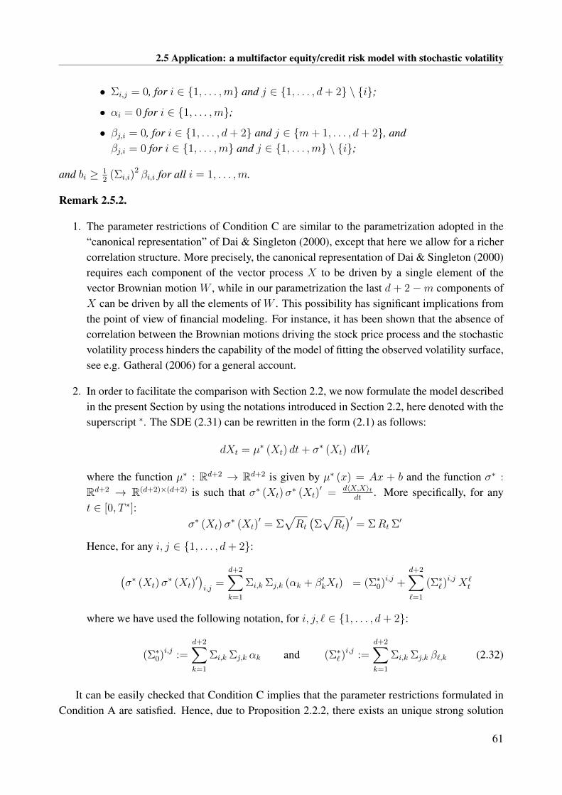
2.5 Application: a multifactor equity/credit risk model with stochastic volatility
• Σi,j = 0, for i ∈ 1, . . . ,m and j ∈ 1, . . . , d+ 2 \ i;
• αi = 0 for i ∈ 1, . . . ,m;
• βj,i = 0, for i ∈ 1, . . . , d+ 2 and j ∈ m+ 1, . . . , d+ 2, andβj,i = 0 for i ∈ 1, . . . ,m and j ∈ 1, . . . ,m \ i;
and bi ≥ 12
(Σi,i)2 βi,i for all i = 1, . . . ,m.
Remark 2.5.2.
1. The parameter restrictions of Condition C are similar to the parametrization adopted in the“canonical representation” of Dai & Singleton (2000), except that here we allow for a richercorrelation structure. More precisely, the canonical representation of Dai & Singleton (2000)requires each component of the vector process X to be driven by a single element of thevector Brownian motion W , while in our parametrization the last d + 2−m components ofX can be driven by all the elements of W . This possibility has significant implications fromthe point of view of financial modeling. For instance, it has been shown that the absence ofcorrelation between the Brownian motions driving the stock price process and the stochasticvolatility process hinders the capability of the model of fitting the observed volatility surface,see e.g. Gatheral (2006) for a general account.
2. In order to facilitate the comparison with Section 2.2, we now formulate the model describedin the present Section by using the notations introduced in Section 2.2, here denoted with thesuperscript ∗. The SDE (2.31) can be rewritten in the form (2.1) as follows:
dXt = µ∗ (Xt) dt+ σ∗ (Xt) dWt
where the function µ∗ : Rd+2 → Rd+2 is given by µ∗ (x) = Ax + b and the function σ∗ :
Rd+2 → R(d+2)×(d+2) is such that σ∗ (Xt)σ∗ (Xt)
′ = d〈X,X〉tdt
. More specifically, for anyt ∈ [0, T ∗]:
σ∗ (Xt)σ∗ (Xt)
′ = Σ√Rt
(Σ√Rt
)′= ΣRt Σ′
Hence, for any i, j ∈ 1, . . . , d+ 2:
(σ∗ (Xt)σ
∗ (Xt)′)i,j
=d+2∑k=1
Σi,k Σj,k (αk + β′kXt) = (Σ∗0)i,j +d+2∑`=1
(Σ∗`)i,j X`
t
where we have used the following notation, for i, j, ` ∈ 1, . . . , d+ 2:
(Σ∗0)i,j :=d+2∑k=1
Σi,k Σj,k αk and (Σ∗`)i,j :=
d+2∑k=1
Σi,k Σj,k β`,k (2.32)
It can be easily checked that Condition C implies that the parameter restrictions formulated inCondition A are satisfied. Hence, due to Proposition 2.2.2, there exists an unique strong solution
61

Chapter 2. Measure changes for reduced-form affine credit risk models
X = (Xt)0≤t≤T ∗ on (Ω,G,F, P ) taking values in Rm++×Rd+2−m to the SDE (2.31). More explicitly,
we have that, for i ∈ 1, . . . ,m:
dX it =
(bi +
m∑j=1
Ai,j Xjt
)dt+ Σi,i
√βi,iX i
t dWit (2.33)
and, for i ∈ m+ 1, . . . , d+ 2:
dX it =
(bi +
d+2∑j=1
Ai,j Xjt
)dt+
m∑j=1
Σi,j
√βj,j X
jt dW
jt +
d+2∑k=m+1
Σi,k
√√√√αk +m∑`=1
β`,kX`t dW
kt
(2.34)By combining (2.22) and (2.34) (for i = d + 2), we can obtain the following dynamics for the
defaultable stock price process S:
dSt = St−
(bd+2 +
1
2
d+2∑k=m+1
(Σd+2,k)2 αk + Ad+2,d+2 logSt−
+
(Ad+2,1 +
1
2(Σd+2,1)2 β11 +
1
2
d+2∑k=m+1
(Σd+2,k)2 β1,k
)vt
+d∑j=1
Ad+2,j+1 Yjt +
1
2
m−1∑j=1
(Σd+2,j+1)2 βj+1,j+1 Yjt
+1
2
d+2∑k=m+1
m−1∑`=1
(Σd+2,k)2 β`+1,k Y
`t
)dt
+ St−Σd+2,1
√β1,1 vt dW
1t + St−
m−1∑j=1
Σd+2,j+1
√βj+1,j+1 Y
jt dW
j+1t
+ St−
d+2∑k=m+1
Σd+2,k
√√√√αk + β1,k vt +m−1∑`=1
β`+1,k Y `t dW
kt − St− dHt
=: St−µS (Xt) dt+ St−
d+2∑j=1
Σd+2,j
√Rj,jt dW j
t − St− dHt
= St−(µS (Xt)− λPt
)dt+ St−
d+2∑j=1
Σd+2,j
√Rj,jt dW j
t − St− dMPt
(2.35)
where MP is the (P,G)-martingale introduced in part (a) of Lemma 2.2.3. As can be immediatelyseen from (2.35), the defaultable stock price process S has rich and flexible stochastic dynamics. Inparticular, the SDE (2.35) allows for stochastic volatility and both the drift and the diffusion termsof S depend on the factor process Y . In addition, the drift term can depend on the volatility and onthe pre-default stock price process itself. Observe that we have three distinct layers of interactionbetween S and the volatility v:
62

2.5 Application: a multifactor equity/credit risk model with stochastic volatility
1. a direct interaction, since v appears explicitly in the dynamics of S;
2. a “semi-direct” interaction, since the Brownian motion W 1 driving the process v is also oneof the drivers in the dynamics of S;
3. an indirect interaction, due to the common dependence of the processes S and v on the factorprocess Y .
The framework so far described is rather general and, in particular, can be regarded as an ex-tension to a defaultable setting of several stochastic volatility models proposed in the literature, asshown in the following Examples.
Example 2.5.3 (The Heston with jump-to-default model). Let us consider the simple case whered = 0 and m = 1, meaning that we do not consider any factor process Y . Let the model parametersbe specified as follows:
b =
(b
µ
)A =
(a 0
−1/2 0
)Σ =
(k 0
ρ√
1− ρ2
)α =
(0
0
)β =
(1 1
0 0
)where b ≥ k2/2, µ, a, k ∈ R and ρ ∈ [−1, 1]. It is easy to check that this parametrization satisfiesCondition C. Due to (2.35), the defaultable stock price process satisfies the following SDE:
dSt = St−µ dt+ St−√vt ρ dW
1t + St−
√vt√
1− ρ2 dW 2 − St− dHt
= St−µ dt+ St−√vt dWt − St− dHt
(2.36)
where the process W =(Wt
)0≤t≤T ∗ is a (P,F)-Brownian motion defined as Wt := ρW 1
t +√1− ρ2W 2
t , for t ∈ [0, T ∗]. The volatility process satisfies the following SDE, as can be easilyseen from (2.33):
dvt =(b+ avt
)dt+ k
√vt dW
1t (2.37)
and d〈W ,W 1〉t = ρ dt. We have thus recovered the Heston with jump-to-default model consideredin Section 2.4. Clearly, we can extend this model by introducing a non-trivial factor process Y , aswill be shown in the next Examples.
Example 2.5.4 (A defaultable two-factor stochastic volatility model). Let d = 1 and m = 2 andconsider the following specification for the model parameters:
A =
−k k 0
0 −k0 0
−1/2 0 0
Σ =
σ 0 0
0 σ0 0
ρ 0√
1− ρ2
β =
1 0 1
0 1 0
0 0 0
b =
(kv, k0y, µ− ζ
)′α = (0, 0, 0)′
with k ∈ R+, k0, v, σ, σ0, µ, ζ ∈ R, kv ≥ σ2/2, k0y ≥ σ20/2 and ρ ∈ [−1, 1]. It is easy to check
that this parametrization satisfies Condition C. As can be deduced from (2.35), the defaultable stockprice process satisfies the following SDE:
dSt = St−(µ− ζ
)dt+ St−
√vt
(ρ dW 1
t +√
1− ρ2 dW 3t
)− St− dHt (2.38)
63

Chapter 2. Measure changes for reduced-form affine credit risk models
where the parameters µ and ζ represent the expected return rate and the dividend yield, respectively.The stochastic volatility process v satisfies the following SDE:
dvt = k (v + Yt − vt) dt+ σ√vt dW
1t (2.39)
The factor Y can be thought of as a long-term stochastic trend component of the volatility processand satisfies the following SDE:
dYt = k0 (y − Yt) dt+ σ0
√Yt dW
2t (2.40)
Equations (2.38)-(2.40) are analogous to the two-factor stochastic volatility model considered inSection 4.3 of Duffie et al. (2000), with the additional feature that the stock price process jumps tozero as soon as the default event occurs.
Example 2.5.5 (A defaultable stochastic volatility - stochastic interest rate model). Let d = 1
and m = 2 and suppose that the real-valued process Y represents the stochastic evolution of therisk-free interest rate. Consider the following specification for the model parameters:
A =
a1 0 0
0 a2 0
−12
12
0
Σ =
k1/ρ1 0 0
0 k2/ρ2 0
1 1 1
β =
ρ21 0 1− ρ2
1
0 ρ22 1− ρ2
2
0 0 0
b = (b1, b2, 0)′ α = (0, 0, 0)′
with a1, a2, k1, k2 ∈ R, b1 ≥ k21/2, b2 ≥ k2
2/2 and ρ1, ρ2 ∈ [−1, 1] \ 0. It is easy to check thatthis parametrization satisfies Condition C. As can be seen from (2.35), the defaultable stock priceprocess satisfies the following SDE:
dSt = St− Yt dt+ St−
(ρ1
√vt dW
1t + ρ2
√Yt dW
2t +
√(1− ρ2
1) vt + (1− ρ22)Yt dW
3t
)− St− dHt
(2.41)and the stochastic volatility process v and the interest rate process Y satisfy the following SDEs,respectively:
dvt = (b1 + a1vt) dt+ k1
√vt dW
1t (2.42)
dYt = (b2 + a2Yt) dt+ k2
√Yt dW
2t (2.43)
Observe that (2.41) can be equivalently written as follows:
dSt− = St− Yt dt+ St−
(√vt dW
1t +
√Yt dW
2t
)− St− dHt (2.44)
where W 1 and W 2 are two Brownian motions such that d〈W 1,W 1〉t = ρ1dt and d〈W 2,W 2〉t =
ρ2dt. Equations (2.42)-(2.44) represent a defaultable version of the stochastic volatility - stochasticinterest rate model proposed by Ahlip & Rutkowski (2009), here extended by allowing the stockprice process to jump to zero as soon as the default event occurs.
64

2.5 Application: a multifactor equity/credit risk model with stochastic volatility
Coming back to our general framework, note that the default intensity λP =(λPt)
0≤t≤T ∗ hasbeen left so far unspecified. Following Section 2.2, we specify λP as follows:
λPt = λP +(ΛP)′Xt for all t ∈ [0, T ∗] (2.45)
with λP ∈R+ and ΛP ∈Rd+2+ with ΛP,i = 0 for all i∈m+ 1, . . . , d+ 2 and λP +
∑mi=1 ΛP,i > 0.
The specification (2.45) ensures that the process λP remains P -a.s. strictly positive, since 0 is anunattainable boundary for the firstm components of the processX (see Proposition 2.2.2). The rea-son why we impose a linear structure on λP lies in the possibility of obtaining analytically tractableformulae for several quantities of interest, as will be shown in Section 2.5.2. It is interesting toobserve that (2.45) allows for a direct dependence of the default intensity on the stochastic volatil-ity v. This is a very important feature, being consistent with several empirical observations whichdocument a link between default risk and volatility risk (see for instance the introduction of Carr &Linetsky (2006) and Gatheral (2006), Chapter 6).
Remark 2.5.6 (On the interaction between the stock price and the default intensity). Note thatthe specification (2.45) for the default intensity does not allow for a direct dependence of λP onthe logarithm of the pre-default stock price L, since the latter may take negative values6. However,we can still capture a stochastic interaction between the default intensity and the stock price. Infact, the dynamics of λP and L both depend on the factor process Y and, furthermore, the diffusionterms in the dynamics of L are also directly correlated with the diffusion terms in the dynamics ofλP .
Let us also specify the risk-free spot interest rate r = (rt)0≤t≤T ∗ as follows:
rt = r + Υ′Xt for all t ∈ [0, T ∗] (2.46)
where r ∈ R and Υ ∈ Rd+2. As in the case of the default intensity process, if we want to ensurenon-negative interest rates, we can impose r ∈ R+ and Υ ∈ Rd+2
+ with Υj = 0 for all j ∈m+ 1, . . . , d+ 2. However, in order to cover the most general case, we do not impose thisrestriction on the interest rate process7. We want to point out that specifications of the type (2.46)are very common in the context of term structure modeling via affine processes: see for instanceDuffie & Kan (1996), Dai & Singleton (2000), Duffee (2002) and Chapter 10 of Filipovic (2009).
Remark 2.5.7.
1. The specifications (2.45)-(2.46) for the default intensity and the interest rate allow the pro-cesses λP and r to be correlated, due to their common dependence on the first m components
6 Clearly, one can let the default intensity λP depend also on the last d+ 2−m components of the vector processX , including the pre-default stock price process L, via quadratic or exponential functions in order to ensure that theprocess λP does not leave the positive orthant, see e.g. Fontana & Runggaldier (2010). However, as will be shownin the following Sections, the affine structure of equations (2.45)-(2.46) is crucial for obtaining explicit formulae forseveral key quantities useful for both risk management as well as pricing applications.
7 Note that, even in the case where the interest rate process r is not restricted to the positive orthant, the probabilityof rt taking negative values can be made almost negligible from a practical point of view by a suitable choice of themean-reversion parameters in the SDE (2.31).
65

Chapter 2. Measure changes for reduced-form affine credit risk models
of the Rd+2-valued process X . Furthermore, all the key elements appearing in our modelenjoy a rich correlation structure, in the sense that the stock price, the stochastic volatility,the default intensity, the interest rate and the factor process Y are all mutually correlated.An analogous structure for both the interest rate and the default intensity has been adoptedin Fontana (2010a) in a multi-firm setting and with the additional inclusion of a rating-basedcomponent in the default intensity specification.
2. The present framework can be extended to a multi-firm setting. In fact, suppose that themarket comprises a number p ∈ N of firms and denote by τ i the random default time ofthe i-th firm, for i = 1, . . . , p. As in Section 9.6 of McNeil et al. (2005), we can modelthe random default times τ ii=1,...,p as conditionally independent doubly stochastic randomtimes with respect to (P,F), with corresponding P -default intensities
λP,ii=1,...,p
, wherethe latter are specified as in (2.45). Let us also denote by Li the logarithm of the pre-defaultstock price process of the i-th firm and, analogously, by vi the stochastic volatility processassociated to the i-th firm, for i = 1, . . . , p. We can then define the Rd+2p-valued processX = (Xt)0≤t≤T ∗ as Xt := (v1
t , . . . , vpt , Y
′t , L
1t , . . . , L
pt )′, for all t ∈ [0, T ∗]. It is easy to
see that if X satisfies an SDE of the form (2.31) and if a suitable version of Condition Cholds, then we can still rely on the powerful results made available by the affine technology.Clearly, this multi-firm framework can accommodate flexible stochastic interactions betweenthe different stock price processes and their stochastic volatilities. In particular, the dynamicsof Li can also depend on vj for j 6= i. Furthermore, the default intensities associated to thedifferent firms are mutually correlated, due to the common dependence of
λP,iti=1,...,p
onthe vector (v1
t , . . . , vpt , Y
′t )′.
2.5.2 Risk management applications
By relying on the affine structure of the general framework described in Section 2.5.1, we shallnow be concerned with some simple computations (under the real-world probability measure P ),which may be of interest in view of risk management applications. Let us start with the followingProposition, which will play a key role in the derivation of most of the results of this Section.
Proposition 2.5.8. Suppose that Condition C holds. Then, there exists an unique solution(Φ (·, u) ,
Ψ (·, u))
: [0, T ∗]→ C× Cd+2 to the following system of Riccati ordinary differential equations:
∂tΦ (t, u) = b′Ψ (t, u) +1
2
d+2∑k=m+1
[Σ′Ψ (t, u)]2k αk − λ
P
Φ (0, u) = 0
∂tΨi (t, u) =d+2∑k=1
Ak,i Ψk (t, u) +1
2[Σ′Ψ (t, u)]
2i βi,i +
1
2
d+2∑k=m+1
[Σ′Ψ (t, u)]2k βi,k − ΛP,i
∂tΨj (t, u) =d+2∑
k=m+1
Ak,j Ψk (t, u)
Ψ (0, u) = u
(2.47)
66

2.5 Application: a multifactor equity/credit risk model with stochastic volatility
for i = 1, . . . ,m and j = m + 1, . . . , d + 2 for the initial condition u = 0. Furthermore, thefollowing holds:
E[e−
∫ Tt λPu du eu
′XT∣∣Ft] = eΦ(T−t,u)+Ψ(T−t,u)′Xt
for any t, T ∈ [0, T ∗] with t ≤ T and for any u ∈ Cd+2 such that there exists an unique solution(Φ(·,R (u)
),Ψ(·,R (u)
)):[0, T
]→ R× Rd+2 to system (2.47) for some T ≥ T .
Proof. The proof relies on the same arguments used in the proof of Theorem 10.4 of Filipovic(2009). Note that condition (a) in Theorem 10.4 of Filipovic (2009) is always satisfied by theprocess λP , i.e. we have E
[exp(−∫ T
0λPu du
)]< ∞ for all T ∈ [0, T ∗], since λP is uniformly
bounded from below by 0, due to (2.45) together with Proposition 2.2.2.
From the risk-management perspective, one of the most important quantities we are interestedin is represented by the Gt-conditional survival probability over a given time horizon [t, T ], with0 ≤ t ≤ T ≤ T ∗. This is the content of the following Corollary, the proof of which relies onProposition 2.5.8.
Corollary 2.5.9. Suppose that Condition C holds. For any t, T ∈ [0, T ∗] with t ≤ T , the Gt-conditional survival probability over the time interval [t, T ] is explicitly given as follows:
P (τ > T | Gt) = (1−Ht) e−A(T−t)−B(T−t)′Xt
where Xt := (X1t , . . . , X
mt )′ and the functions A : [0, T ∗] → R and B : [0, T ∗] → Rm are the
unique solutions to the following system of Riccati ordinary differential equations:
∂tA (t) = b′B (t)− 1
2
d+2∑k=m+1
[Σ′B (t)]2k αk + λP
A (0) = 0
∂tBi (t) =d+2∑k=1
Ak,iBk (t)− 1
2[Σ′B (t)]
2i βi,i −
1
2
d+2∑k=m+1
[Σ′B (t)]2k βi,k + ΛP,i
B (0) = 0
(2.48)
for i = 1, . . . ,m.
Proof. Observe first that system (2.48) corresponds to (2.47) with initial condition u = 0 by lettingΦ (t, 0) = −A (t) and Ψi (t, 0) = −Bi (t) for i = 1, . . . ,m. Due to Proposition 2.5.8, there existsan unique solution
(Φ (·, u) ,Ψ (·, u)
): [0, T ∗] → R × Rd+2 to system (2.47) for u = 0. It is also
easy to see that we have Ψj (t, 0) = 0 for all t ∈ [0, T ∗] and j = m + 1, . . . , d + 2. Hence, thereexists an unique solution
(A (·) , B (·)
): [0, T ∗]→ R× Rm to (2.48). We have then:
P (τ > T | Gt) = (1−Ht)P (τ > T |Ft)P (τ > t|Ft)
= (1−Ht)E[e−
∫ Tt λPu du
∣∣Ft]= (1−Ht) e
−A(T−t)−B(T−t)′Xt
where the first two equalities follow from Lemma 5.1.2 and formula (5.9) of Bielecki & Rutkowski(2002) and the last equality follows from Proposition 2.5.8 with u = 0.
67

Chapter 2. Measure changes for reduced-form affine credit risk models
In particular, note that the Gt-conditional survival probability depends only on the first m com-ponents of Xt, i.e. on the components of X which drive the default intensity itself. For T ∈ [0, T ∗],let us now introduce a probability measure P T on (Ω,G), named T -survival probability measureand formally defined as follows8:
dP T
dP:=
e−∫ T0 λPu du
E[e−
∫ T0 λPu du
] (2.49)
The terminology T -survival probability measure is justified by the following property, which holdsfor any integrable FT ∗-measurable random variable F and for any t, T ∈ [0, T ∗] with t ≤ T :
E[F 1τ>T|Gt
]= (1−Ht)
E[F 1τ>T|Ft
]P (τ > t|Ft)
= (1−Ht)E[F E
[1τ>T|FT ∗
]∣∣Ft]P (τ > t|Ft)
= (1−Ht)E[F E
[1τ>T|FT
]∣∣Ft]P (τ > t|Ft)
= (1−Ht)E[e−
∫ T0 λPu du F
∣∣Ft]P (τ > t|Ft)
= (1−Ht)E[e−
∫ Tt λPu du F
∣∣Ft] = (1−Ht)E[e−
∫ Tt λPu du
∣∣Ft]EPT [F |Ft]
= P (τ > T | Gt)EPT [F |Ft](2.50)
where EPT [·] denotes the expectation with respect to P T . In (2.50), the first equality followsfrom Lemma 5.1.2 of Bielecki & Rutkowski (2002), the third equality uses the property thatP (τ > t|Ft) = P (τ > t|Fs) for any s ≥ t (see part 2 of Remark 2.2.4), the sixth equality followsfrom the definition of the measure P T and Bayes’ formula and, finally, the last equality followsas in the proof of Corollary 2.5.9. Hence, we see that the computation of the Gt-conditional ex-pectation of the FT ∗-measurable random variable F in the case of survival until T reduces to thecomputation of the Ft-conditional expectation of the random variable F with respect to the mea-sure P T , while the term P (τ > T | Gt) can be computed as in Corollary 2.5.9. The next Corollarygives an explicit formula for the Ft-conditional characteristic function of the random vector XT
under the T -survival measure P T , for any t, T ∈ [0, T ∗] with t ≤ T .
Corollary 2.5.10. Suppose that Condition C holds. Then, for any t, T ∈ [0, T ∗] with t ≤ T , theFt-conditional characteristic function of the random vector XT with respect to the measure P T isexplicitly given as follows, for all u ∈ iRd+2:
EPT[eu′XT∣∣Ft] =
eΦ(T−t,u)+Ψ(T−t,u)′Xt
e−A(T−t)−B(T−t)′Xt
Proof. Due to the definition of the measure P T we have that:
EPT[eu′XT∣∣Ft] =
E[e−
∫ Tt λPs ds eu
′XT∣∣Ft]
E[e−
∫ Tt λPs ds
∣∣Ft]8 The T -survival probability measure PT bears resemblance to the restricted defaultable forward measure intro-
duced in Bielecki & Rutkowski (2002), Section 15.2.2, except that here PT is defined with respect to the physicalprobability measure P and not with respect to a risk-neutral T -forward probability measure. Compare also the defini-tion of the T -forward survival risk-neutral measure QT in Section 2.5.3.
68

2.5 Application: a multifactor equity/credit risk model with stochastic volatility
The claim then follows by applying Proposition 2.5.8 (and Corollary 2.5.9) with u ∈ iRd+2 andu = 0 to the numerator and to the denominator, respectively.
Due to (2.50), we can compute the Gt-conditional expectation (under the real-world probabilitymeasure P ) of arbitrary functions of the random vector XT in the case of survival by relying onCorollaries 2.5.9 and 2.5.10 and employing standard Fourier inversion techniques (for a specificapplication, see Proposition 2.5.12).
Remark 2.5.11. For any t, T ∈ [0, T ∗] with t ≤ T , we have derived in Corollary 2.5.10 the Ft-conditional characteristic function of the random vector XT with respect to the T -survival measureP T . It is worth pointing out that the Ft-conditional characteristic function also coincides with theGt-conditional characteristic function, i.e.:
EPT[eu′XT∣∣Gt] = EPT
[eu′XT∣∣Ft] =
eΦ(T−t,u)+Ψ(T−t,u)′Xt
e−A(T−t)−B(T−t)′Xt
To prove the first equality, recall that the immersion property holds under the measure P , dueto part (b) of Lemma 2.2.3. Since the density dPT
dPof the measure P T with respect to P is FT -
measurable, being λP an F-adapted process, Proposition 5.9.1.2 of Jeanblanc et al. (2009) impliesthat the immersion property holds also with respect to the measure P T . Hence, due to Proposition5.9.1.1 of Jeanblanc et al. (2009), we obtain that EPT
[eu′XT | Gt
]= EPT
[eu′XT |Ft
], since XT is
FT -measurable.
Many risk management applications (like the computation of Value-at-Risk or similar risk mea-sures) require the knowledge of quantiles of the conditional distribution (under the real-world mea-sure P ) of the defaultable stock price at a given future time. To this effect, we derive in the followingProposition the Gt-conditional distribution function of the defaultable stock price at time T in thecase of survival.
Proposition 2.5.12. Suppose that Condition C holds. Let x ∈ R+ and t, T ∈ [0, T ∗] with t ≤ T .Then the following hold:
P (ST ≤ x, τ > T | Gt) = (1−Ht) e−A(T−t)−B(T−t)′Xt
(1
2− 1
π
∫ ∞0
Im(e−iy log x ϕTt (y)
)y
dy
)
where Im denotes the imaginary part and ϕTt denotes the Ft-conditional characteristic function ofLT under the measure P T , explicitly given as follows:
ϕTt (y) := EPT[e iyLT |Ft
]=eΦ(T−t,iyd+2)+Ψ(T−t,iyd+2)′Xt
e−A(T−t)−B(T−t)′Xt
for all y ∈ R and where yd+2 denotes the vector (0, . . . , 0, y)′ ∈ Rd+2.
Proof. Observe first that:
P (ST ≤ x, τ > T |Gt) = P (LT ≤ log x, τ > T |Gt) = P (τ > T |Gt)P T (LT ≤ log x|Ft)
= (1−Ht) e−A(T−t)−B(T−t)′Xt P T (LT ≤ log x|Ft)
69

Chapter 2. Measure changes for reduced-form affine credit risk models
where the second equality follows from (2.50) and the third equality from Corollary 2.5.9. Byrelying on standard Fourier inversion techniques, it can be shown that (see e.g. Paolella (2007),Section 1.2.6):
P T (LT ≤ log x|Ft) =1
2− 1
π
∫ ∞0
Im(e−iy log x ϕTt (y)
)y
dy
where Im denotes the imaginary part and ϕTt denotes the Ft-conditional characteristic functionof LT under the measure P T . The latter can be determined by relying on Corollary 2.5.10, withu = i (0, . . . , 0, y)′ =: iyd+2 ∈ iRd+2.
2.5.3 Risk-neutral measures and valuation of default-sensitive payoffs
In Section 2.5.1, we have described the modeling framework with respect to the probability measureP , which represents the probability measure characterizing the physical world. Accordingly, wehave considered in Section 2.5.2 several risk management applications, always under the real-world measure P . However, if we want to proceed with the arbitrage-free valuation of financialderivatives, we need to shift the model to a proper risk-neutral measure. As in Section 2.4.2, letus denote by S =
(St)
0≤t≤T ∗ the discounted stock price process, where St := e−∫ t0 ruduSt for all
t ∈ [0, T ∗]. A probability measure Q on (Ω,G) with Q ∼ P is said to be an Equivalent LocalMartingale Measure (ELMM) (or risk-neutral measure) for S if the process S is a (Q,G)-localmartingale. It is well-known that the existence of an ELMM for S is equivalent to the No FreeLunch with Vanishing Risk no-arbitrage condition. This follows from the fundamental theorem ofasset pricing in the version of Delbaen & Schachermayer (1994), since S is locally bounded9.
It is important to be aware of the fact that most of the key features of the modeling frameworkdescribed in Section 2.5.1 are not necessarily preserved by an equivalent change of measure. Inparticular, the affine structure of (X, τ), in the sense of Definition 2.2.5, may be lost. However, thegeneral results of Section 2.3 allow us to formulate conditions on the density process of an ELMMso that the affine structure of (X, τ) is preserved.
Proposition 2.5.13. Suppose that Condition C holds. Let θ = (θt)0≤t≤T ∗ be an Rd+2-valued pro-cess satisfying the following condition, for all t ∈ [0, T ∗]:
θt = θ (Xt) :=(√
Rt
)−1 (θ + ΘXt
)(2.51)
for some θ ∈ Rd+2 and Θ ∈ R(d+2)×(d+2) such that:
(i)∑d+2
k=1 Σi,kθk ≥ 12
(Σ i,i)2 βi,i − bi for all i ∈ 1, . . . ,m;
(ii)∑d+2
k=1 Σi,kΘk,j = 0, for all i ∈ 1, . . . ,m and j ∈ m+ 1, . . . , d+ 2,and
∑d+2k=1 Σi,kΘk,j ≥ −Ai,j , for all i ∈ 1, . . . ,m and j ∈ 1, . . . ,m \ i.
9In fact, S is non-negative and bounded from above by the discounted pre-default stock price process e−∫ ·0rudu S,
which, being continuous, is locally bounded.
70

2.5 Application: a multifactor equity/credit risk model with stochastic volatility
Let γ = (γt)0≤t≤T ∗ be a real-valued process satisfying the following condition, for all t ∈ [0, T ∗]:
γt = γ (Xt) :=
(λQ − λP
)+(ΛQ − ΛP
)′Xt
λP + (ΛP )′Xt
(2.52)
for some λQ ∈ R+ and ΛQ ∈ Rd+2+ with ΛQ,i = 0 for all i ∈ m+ 1, . . . , d+ 2 and λQ +∑m
i=1 ΛQ,i > 0 and where λP and ΛP are as in (2.45). Furthermore, suppose that the followingidentity holds P -a.s. on [0, T ∗ ∧ τ ]:
µS (Xt)− λPt (1 + γt) +d+2∑j=1
Σd+2,j
√Rj,jt θjt = rt (2.53)
where the function µS : Rd+2 → R is as in (2.35). Then the measure Q on (Ω,G) defined bydQdP
:= E(∫
θ′dW +∫γ dMP
)T ∗
is an ELMM for S which preserves the affine structure of (X, τ).
Proof. Note that conditions (2.51)-(2.52) are analogous to conditions (2.8)-(2.9) for the affine pro-cess X as given in (2.31). Theorem 2.3.7 implies that E
(∫θ′dW +
∫γ dMP
)is a P -a.s. strictly
positive (P,G)-martingale on [0, T ∗] and, hence, we can define a measure Q on (Ω,G) with Q ∼ P
by letting dQdP
:= E(∫
θ′dW +∫γ dMP
)T ∗
. Theorem 2.3.12 shows that Q preserves the affinestructure of (X, τ). Finally, Girsanov’s theorem and (2.53) imply that S is a (Q,G)-local martin-gale. In fact, recalling equation (2.35):
dSt = St−(µS (Xt)− λPt − rt
)dt+ St−
d+2∑j=1
Σd+2,j
√Rj,jt dW j
t − St− dMPt
= St−
(µS (Xt)− λPt − rt +
d+2∑j=1
Σd+2,j
√Rj,jt θ
jt − λPt γt
)dt+ St−
d+2∑j=1
Σd+2,j
√Rj,jt dWQ,j
t
− St− dMQt
= St−
d+2∑j=1
Σd+2,j
√Rj,jt dWQ,j
t − St− dMQt
where WQ =(WQt
)0≤t≤T ∗ is the (Q,F)/(Q,G)-Brownian motion defined by WQ := W −
∫ ·0θudu
and MQ =(MQ
t
)0≤t≤T ∗ is the (Q,G)-martingale defined by MQ := MP −
∫ ·∧τ0
λPu γudu.
Remark 2.5.14 (On diffusive and jump-type risk premia). The processes θ and γ admit thefinancial interpretation of risk premia associated to the randomness generated by W and MP , re-spectively. The Rd+2-valued process θ represents the risk premium associated to the “diffusiverisk” generated by the randomness driving the process X . Since the stock price, the volatility,the interest rate and the default intensity all depend on X , the risk premium θ can be consideredas a market-wide non-diversifiable risk premium. The real-valued process γ represents the riskpremium associated to the default event or, more precisely, the risk premium associated to the id-iosyncratic component of the risk generated by the occurrence of the default event (see also El
71

Chapter 2. Measure changes for reduced-form affine credit risk models
Karoui & Martellini (2001) and Campi et al. (2009)). Assuming γ ≡ 0 means that the idiosyn-cratic component of the default risk can be diversified away in the market, as explained in Jarrowet al. (2005), and, therefore, market participants do not require a compensation for it. However,since we are considering a single firm, assuming γ ≡ 0 may be seen as an over-simplification ofthe model. Indeed, it is reasonable to expect the jump-type risk premium to be large when it isdifficult to hedge the risk associated with the timing of the default event of a particular firm. As canbe immediately seen from (2.51)-(2.52), the risk premia θ and γ are not independent, due to theircommon dependence on X . Finally, as we have pointed out at the beginning of Section 2.5.1, thelast d− d− 2 components of the Rd-valued Brownian motion W will only be used in Section 2.5.4to model noise factors affecting the observations of market data. Consequently, it seems reasonableto assume that such “noise-related risk” does not carry any intrinsic financial risk and can be diver-sified away. Consequently, market participants do not require a compensation for being exposed tothe randomness generated by the last d− d− 2 components of the Brownian motion W .
Until the end of this Section, we shall always assume that the hypotheses of Proposition 2.5.13hold and, hence, there exists a risk-neutral measureQwhich preserves the affine structure of (X, τ).This implies that the process X satisfies the following SDE on (Ω,G,F, Q):
dXt =(bQ + AQXt
)dt+ Σ
√Rt dW
Qt (2.54)
where bQ ∈ Rd+2 and AQ ∈ R(d+2)×(d+2) are defined as follows, for i, j ∈ 1, . . . , d+ 2:
AQi,j := Ai,j +d+2∑k=1
Σi,kΘk,j and bQi := bi +d+2∑k=1
Σi,kθk (2.55)
For the purpose of valuing default-sensitive payoffs, the T -forward survival risk-neutral prob-ability measure QT turns out to be useful. For any T ∈ [0, T ∗], the measure QT is defined asfollows10:
dQT
dQ=
e−∫ T0 (ru+λQu ) du
EQ[e−
∫ T0 (ru+λQu )du
] (2.56)
where EQ [·] denotes the expectation with respect to the risk-neutral measure Q. The measure QT
bears resemblance to the T -survival measure P T introduced in Section 2.5.2, except that QT isdefined with respect to a risk-neutral measure Q and the density dQT
dQalso involves the discount
factor.In the following Proposition, we derive a general formula for the arbitrage-free price of a general
payoff with maturity T ∈ [0, T ∗], paid only if the default event occurs after T . We call this situationthe zero recovery case.
10We assume throughout this Section that EQ[e−
∫ T0rudu
]<∞ for all T ∈ [0, T ∗]. Clearly, under this assumption
the expectation appearing in the denominator of (2.56) is finite.
72

2.5 Application: a multifactor equity/credit risk model with stochastic volatility
Proposition 2.5.15. Let t, T ∈ [0, T ∗] with t ≤ T and let F : Rd+2 → R+. Then the arbitrage-freeprice at time t of the random payoff F (XT ) at maturity T on the event τ > T, with zero recoveryin the case of default, is given by the following expression:
EQ[e−
∫ Tt rudu F (XT ) (1−HT )
∣∣Gt] = (1−Ht)EQ[e−
∫ Tt (ru+λQu )du∣∣Ft]EQT [F (XT ) |Ft]
(2.57)
Proof. Since the random variable e−∫ Tt ruduF (XT ) is FT -measurable, Corollary 5.1.1 of Bielecki
& Rutkowski (2002) implies that:
E Q[e−
∫ Tt ruduF (XT ) (1−HT )
∣∣Gt] = (1−Ht)EQ[e−
∫ Tt (ru+λQu )duF (XT )
∣∣Ft]Equation (2.57) follows then immediately from the definition of QT and Bayes’ rule.
The next Proposition deals with the arbitrage-free valuation of a recovery payment, i.e. a payoffwhich is paid exactly at the time of default if the latter occurs before a fixed maturity T ∈ [0, T ∗].
Proposition 2.5.16. Let t, T ∈ [0, T ∗] with t ≤ T and let G : Rd+2 → R+. Then the arbitrage-freeprice at time t of the random payoff G (Xτ ) at the default time τ on the event τ ≤ T is given bythe following expression:
EQ[e−
∫ τ0 ruduG (Xτ )1t<τ≤T
∣∣Gt] = (1−Ht)
∫ T
t
EQ[e−
∫ ut (rs+λQs )ds∣∣Ft]EQu
[λQu G (Xu) |Ft
]du
(2.58)
Proof. Corollary 5.1.3 of Bielecki & Rutkowski (2002) implies that:
EQ[e−
∫ τ0 ruduG (Xτ )1t<τ≤T
∣∣Gt] = (1−Ht)EQ
[∫ T
t
e−∫ ut (rs+λQs )ds λQu G (Xu) du
∣∣∣Ft]Equation (2.58) then easily follows by first applying Tonelli’s theorem and then using the definitionof the u-forward survival risk-neutral measure Qu and Bayes’ rule.
Remark 2.5.17. In the particular case where G ≡ δ for some δ ∈ (0,∞), one can obtain analternative formula for the recovery payment in terms of defaultable forward rates and forwardhazard rates conditioned on survival: see Lemma 2.1 of Fontana & Runggaldier (2010).
By combining Propositions 2.5.15 and 2.5.16 we can obtain the arbitrage-free price of a genericdefaultable claim which pays a random amount at maturity in the case of survival and a randomrecovery at the time of default if the latter occurs before the maturity. Most (single-name) creditderivatives can be written as linear combinations of zero-recovery contingent claims and a purerecovery contingent claim, the latter being paid only in the case of default. Note that Propositions2.5.15 and 2.5.16 do not rely on the affine structure of (X, τ). As can be seen from (2.57)-(2.58), ifwe want to obtain more explicit results, we need to be able to compute the two following quantities:
1. theFt-conditional expected value (underQ) of random variables of the form exp(−∫ Tt
(λQu +
ru)du), for t, T ∈ [0, T ∗] with t ≤ T ;
73

Chapter 2. Measure changes for reduced-form affine credit risk models
2. the Ft-conditional expected value (under QT ) of random variables of the form Γ (XT ), forsome function Γ : Rd+2 → R+ and t, T ∈ [0, T ∗] with t ≤ T .
Due to the affine structure of (X, τ) under the measure Q, the first of the above two elements canbe computed in closed form. Furthermore, we are able to obtain an explicit expression for theFt-conditional characteristic function of XT under the measure QT and, hence, we can computeEQT [Γ (XT ) |Ft] by relying on standard Fourier inversion techniques, see e.g. Carr & Madan(1999).
Proposition 2.5.18. Let t, T ∈ [0, T ∗] with t ≤ T . Then the following hold:
(a) EQ[e−
∫ Tt (ru+λQu )du∣∣Ft] = eΦQ(T−t,0)+ΨQ(T−t,0)′Xt
(b) the Ft-conditional characteristic function of XT with respect to QT is explicitly given asfollows, for all u ∈ iRd+2:
EQT[eu′XT∣∣Ft] =
eΦQ(T−t,u)+ΨQ(T−t,u)′Xt
eΦQ(T−t,0)+ΨQ(T−t,0)′Xt(2.59)
where the functions ΦQ : [0, T ∗]×Cd+2 → C and ΨQ : [0, T ∗]×Cd+2 → Cd+2 solve the followingsystem of Riccati ordinary differential equations:
∂tΦQ (t, u) =
(bQ)′
ΨQ (t, u) +1
2
d+2∑k=m+1
[Σ′ΨQ (t, u)
]2kαk − r − λQ
ΦQ (0, u) = 0
∂tΨQi (t, u) =
d+2∑k=1
AQk,i ΨQk (t, u) +
1
2
[Σ′ΨQ (t, u)
]2iβi,i +
1
2
d+2∑k=m+1
[Σ′ΨQ (t, u)
]2kβi,k −Υi − ΛQ,i
∂tΨQj (t, u) =
d+2∑k=m+1
AQk,j ΨQk (t, u)−Υj
ΨQ (0, u) = u(2.60)
for i = 1, . . . ,m and j = m + 1, . . . , d + 2, where the parameters AQ and bQ are defined as in(2.55), the parameters r and Υ as in (2.46) and the parameters λQ and ΛQ as in (2.52).
Proof. Recalling that in this Section we always assume that the hypotheses of Proposition 2.5.13hold, the tuple
(AQ, bQ,Σ, α, β
)satisfies Condition C. Therefore, part (a) of the Proposition can
be proved by relying on the same arguments used in the proof of Proposition 2.5.8 and Corollary2.5.9, now with respect to the measureQ, and part (b) by relying on Proposition 2.5.8 and Corollary2.5.10, using also the definition of the T -forward survival risk-neutral measure QT . Analogousresults are given in Theorem 10.4 and Corollary 10.2 of Filipovic (2009).
74

2.5 Application: a multifactor equity/credit risk model with stochastic volatility
Risk-neutral valuation of fixed-income defaultable products
By relying on Propositions 2.5.15, 2.5.16 and 2.5.18, we can now proceed to the arbitrage-freevaluation of some typical payoffs. The following Corollary deals with the valuation of default-free0-coupon bonds and defaultable 0-coupon 0-recovery bonds, with unitary face value. It is well-known that these elementary financial products can be considered as the building blocks of morecomplex financial derivatives. In the following Corollary, the subscript “rf ” stands for “risk-free”while “df ” stands for “defaultable”.
Corollary 2.5.19. Let t, T ∈ [0, T ∗] with t ≤ T . Then the following hold:
(a) the arbitrage-free price at time t of a 0-coupon default-free bond with maturity T is given bythe following expression:
Πrf (t, T ) := EQ[e−
∫ Tt rudu
∣∣Gt] = eΦQ(T−t,0)+ΨQ(T−t,0)′Xt
where the functions ΦQ : [0, T ∗] × Cd+2 → C and ΨQ : [0, T ∗] × Cd+2 → Cd+2 satisfy asystem of Riccati ODEs of the type (2.60) but without the parameters λQ and ΛQ;
(b) the arbitrage-free price at time t of a 0-coupon 0-recovery defaultable bond with maturity Tis given by the following expression:
Πdf (t, T ) := EQ[e−
∫ Tt rudu (1−HT )
∣∣Gt] = (1−Ht) eΦQ(T−t,0)+ΨQ(T−t,0)′Xt
where the functions ΦQ : [0, T ∗] × Cd+2 → C and ΨQ : [0, T ∗] × Cd+2 → Cd+2 satisfy thesystem of Riccati ODEs (2.60).
Proof. To prove part (a), note that EQ[e−
∫ Tt rudu
∣∣Gt] = EQ[e−
∫ Tt rudu
∣∣Ft], due to the immersionproperty between the filtrations F and G under Q (see part (a) of Theorem 2.3.10) together withProposition 5.9.1.1 of Jeanblanc et al. (2009). Since the interest rate process r is linear with respectto X , due to (2.46), and since X satisfies on (Ω,G,F, Q) the SDE (2.54), part (a) can be proved asthe first part of Corollary 10.2 of Filipovic (2009). To prove part (b) it suffices to use Proposition2.5.15 (with F ≡ 1) together with part (a) of Proposition 2.5.18.
The following Definition formalizes the well-known concepts of yield of a 0-coupon default-free bond and credit spread of a 0-coupon 0-recovery defaultable bond.
Definition 2.5.20. Let t, T ∈ [0, T ∗] with t < T :
• the yield Y L (t, T ) of a 0-coupon default-free bond is defined as follows:
Y L (t, T ) := − 1
T − tlog(Πrf (t, T )
)• the credit spreadCS (t, T ) of a 0-coupon 0-recovery defaultable bond, computed with respect
to a 0-coupon default-free bond with the same maturity T , is defined as follows on the setτ > t:
CS (t, T ) := − 1
T − tlog
(Πdf (t, T )
Πrf (t, T )
)
75

Chapter 2. Measure changes for reduced-form affine credit risk models
It is obvious that, due to Corollary 2.5.19, yields and credit spreads take the following linearform:
Y L (t, T ) = −ΦQ (T − t, 0)
T − t− ΨQ (T − t, 0)′
T − tXt
=: AY L (T − t) +BY L (T − t)′Xt
(2.61)
and, on the set τ > t:
CS (t, T ) =ΦQ (T − t, 0)− ΦQ (T − t, 0)
T − t+
(ΨQ (T − t, 0)−ΨQ (T − t, 0)
)′T − t
Xt
=: ACS (T − t) +BCS (T − t)′Xt
(2.62)
By relying on Corollary 2.5.19, we can easily compute the arbitrage-free prices of default-freeand defaultable coupon-bearing bonds: see for instance Bielecki & Rutkowski (2002), Section1.1.5. By combining Corollary 2.5.19 with Proposition 2.5.16, we can also value defaultable cor-porate bonds with non-zero recovery payments in the case of default. Furthermore, these resultsallow us to compute the fair spread of a Credit Default Swap (see e.g. Fontana & Runggaldier(2010), Section 2.2).
Risk-neutral valuation of equity-related defaultable products
While Corollary 2.5.19 deals with the valuation of fixed-income default-free and defaultable finan-cial products, let us now consider the case of equity-related products. In particular, we now derivesemi-explicit formulae for the arbitrage-free prices of call and put options written on the default-able stock S. In the following Corollary we assume that the options are issued by the defaultablefirm itself and written on its own stock S, with zero recovery in the case of default. This means thatif the firm goes bankrupt before the maturity of the option then the latter becomes worthless.
Corollary 2.5.21. Let t, T ∈ [0, T ∗] with t ≤ T and let K ∈ (0,∞) denote a fixed strike price.Then the following hold11:
(a) the arbitrage-free price at time t of an European call option issued by the defaultable firmitself and written on S, with maturity T and strike price K, is given by the following expres-sion:
CK (t, T ) := EQ[e−
∫ Tt rudu (ST −K)+ (1−HT )
∣∣Gt]= (1−Ht) e
ΦQ(T−t,0)+ΨQ(T−t,0)′Xt1
2π
∫ +∞
−∞ϕTt (w + iu)
K−(w−1+iu)
(w + iu) (w − 1 + iu)du
(2.63)for some w ∈ (1,∞) such that the system of Riccati ODEs (2.60) has an unique solution withinitial condition u = (0, . . . , 0, w)′ ∈ Rd+2;
11Observe that the only difference between the risk-neutral valuation formulae (2.63) and (2.64) lies in the intervalthe fixed parameter w belongs to.
76
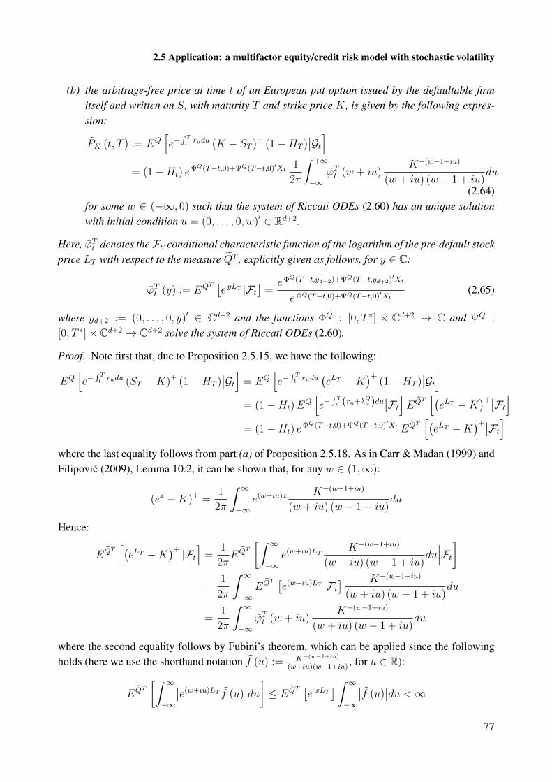
2.5 Application: a multifactor equity/credit risk model with stochastic volatility
(b) the arbitrage-free price at time t of an European put option issued by the defaultable firmitself and written on S, with maturity T and strike price K, is given by the following expres-sion:
PK (t, T ) := EQ[e−
∫ Tt rudu (K − ST )+ (1−HT )
∣∣Gt]= (1−Ht) e
ΦQ(T−t,0)+ΨQ(T−t,0)′Xt1
2π
∫ +∞
−∞ϕTt (w + iu)
K−(w−1+iu)
(w + iu) (w − 1 + iu)du
(2.64)for some w ∈ (−∞, 0) such that the system of Riccati ODEs (2.60) has an unique solutionwith initial condition u = (0, . . . , 0, w)′ ∈ Rd+2.
Here, ϕTt denotes theFt-conditional characteristic function of the logarithm of the pre-default stockprice LT with respect to the measure QT , explicitly given as follows, for y ∈ C:
ϕTt (y) := EQT[e yLT |Ft
]=eΦQ(T−t,yd+2)+ΨQ(T−t,yd+2)′Xt
eΦQ(T−t,0)+ΨQ(T−t,0)′Xt(2.65)
where yd+2 := (0, . . . , 0, y)′ ∈ Cd+2 and the functions ΦQ : [0, T ∗] × Cd+2 → C and ΨQ :
[0, T ∗]× Cd+2 → Cd+2 solve the system of Riccati ODEs (2.60).
Proof. Note first that, due to Proposition 2.5.15, we have the following:
EQ[e−
∫ Tt rudu (ST −K)+ (1−HT )
∣∣Gt] = EQ[e−
∫ Tt rudu
(eLT −K
)+(1−HT )
∣∣Gt]= (1−Ht)E
Q[e−
∫ Tt (ru+λQu )du∣∣Ft]EQT
[(eLT −K
)+∣∣Ft]= (1−Ht) e
ΦQ(T−t,0)+ΨQ(T−t,0)′Xt EQT[(eLT −K
)+∣∣Ft]where the last equality follows from part (a) of Proposition 2.5.18. As in Carr & Madan (1999) andFilipovic (2009), Lemma 10.2, it can be shown that, for any w ∈ (1,∞):
(ex −K)+ =1
2π
∫ ∞−∞
e(w+iu)x K−(w−1+iu)
(w + iu) (w − 1 + iu)du
Hence:
EQT[(eLT −K
)+ |Ft]
=1
2πEQT
[∫ ∞−∞
e(w+iu)LTK−(w−1+iu)
(w + iu) (w − 1 + iu)du∣∣∣Ft]
=1
2π
∫ ∞−∞
EQT[e(w+iu)LT |Ft
] K−(w−1+iu)
(w + iu) (w − 1 + iu)du
=1
2π
∫ ∞−∞
ϕTt (w + iu)K−(w−1+iu)
(w + iu) (w − 1 + iu)du
where the second equality follows by Fubini’s theorem, which can be applied since the followingholds (here we use the shorthand notation f (u) := K−(w−1+iu)
(w+iu)(w−1+iu), for u ∈ R):
EQT[∫ ∞−∞
∣∣e(w+iu)LT f (u)∣∣du] ≤ EQT
[ewLT
] ∫ ∞−∞
∣∣f (u)∣∣du <∞
77

Chapter 2. Measure changes for reduced-form affine credit risk models
due to the fact that the function f is integrable and w ∈ (1,∞) is such that there exists an uniquesolution to the system of Riccati ODEs (2.60) with initial condition u = (0, . . . , 0, w)′ ∈ Rd+2
(see also Filipovic (2009), Theorem 10.5). The explicit expression given in equation (2.65) forthe Ft-conditional characteristic function of LT under the measure QT follows from part (b) ofProposition 2.5.18. This completes the proof of part (a) of the Corollary. Part (b) can be proved ina similar way, using the fact that, for w ∈ (−∞, 0):
(K − ex) =1
2π
∫ ∞−∞
e(w+iu)x K−(w−1+iu)
(w + iu) (w − 1 + iu)du
By relying on techniques similar to those used in the proof of Corollary 2.5.21 and exploiting theknowledge of the Ft-conditional characteristic function of XT with respect to QT , one can derivethe arbitrage-free value of more complex payoffs, see e.g. Section 10.3.1 of Filipovic (2009).
We want to remark that, since the defaultable stock price process jumps to zero as soon as thedefault event occurs and remains thereafter frozen at zero, we have that:
CK (t, T ) = EQ[e−
∫ Tt rudu (ST −K)+ (1−HT )
∣∣Gt]= EQ
[e−
∫ Tt rudu (ST −K)+
∣∣Gt] =: CK (t, T )(2.66)
As in Corollary 2.5.21, CK (t, T ) denotes the arbitrage-free price of a call option issued by thedefaultable firm itself. On the contrary, CK (t, T ) denotes the arbitrage-free price of a call optionwritten on the defaultable stock S but issued by a default-free third party12. Hence, (2.66) showsthat the arbitrage-free price of an European call option written on S does not depend on whetherit is issued by the defaultable firm itself or by a default-free third party. This is intuitively clear.In fact, both options are written on the same defaultable stock S and, since the process S remainsfrozen at zero as soon as the default event occurs, a call option becomes worthless as soon as thedefault event occurs regardless of the fact that the option is issued by the defaultable firm itselfor by a default-free third party. However, this is not the case for a put option. In fact, part (b) ofCorollary 2.5.21 gives the arbitrage-free price of an European put option, with strike price K andmaturity T , issued by the defaultable firm itself. If we consider instead a put option (with the samestrike price K and maturity T ) written on the defaultable stock S but issued by a default-free thirdparty and not by the defaultable firm itself, then it has to be valued as follows:
PK (t, T ) := EQ[e−
∫ Tt rudu (K − ST )+
∣∣Gt]= EQ
[e−
∫ Tt rudu (K − ST )+ (1−HT )
∣∣Gt]+K EQ[e−
∫ Tt ruduHT
∣∣Gt]= PK (t, T ) +K EQ
[e−
∫ Tt ruduHT
∣∣Gt](2.67)
12 We distinguish arbitrage-free prices of options issued by a default-free third party and written on the defaultablestock S from arbitrage-free prices of options issued by the defaultable firm itself and written on its own stock S byusing the tilde notation for the latter.
78

2.5 Application: a multifactor equity/credit risk model with stochastic volatility
We can notice that the arbitrage-free price of a put option issued by a default-free third party can bedecomposed into the sum of the arbitrage-free price of a put option issued by the defaultable firmitself and an additional term equal to the arbitrage-free value at time t of the payment of the strikeprice K at the maturity T if the firm defaults before time T . Let us focus on this last term:
EQ[e−
∫ Tt ruduHT
∣∣Gt] = EQ[e−
∫ Tt rudu (1− 1 +HT )
∣∣Gt]= EQ
[e−
∫ Tt rudu
∣∣Gt]− EQ[e−
∫ Tt rudu (1−HT )
∣∣Gt]= Πrf (t, T )− Πdf (t, T ) > 0
(2.68)
where we have used the definition of Πrf (t, T ) and Πdf (t, T ) (compare Corollary 2.5.19). Wehave thus shown that, in line with the economic intuition, the arbitrage-free price PK (t, T ) of a putoption issued by a default-free third party can be decomposed into the sum of the price PK (t, T )
of a put option with identical characteristics (in terms of underlying, strike price and maturity) butissued by the defaultable firm itself and a “default-protection” term proportional to the difference(Πrf (t, T ) − Πdf (t, T )
)between the arbitrage-free prices of a 0-coupon default-free bond and of
a 0-coupon 0-recovery defaultable bond.Similarly as in Chapter 6 of Gatheral (2006), we can easily derive the following put-call parity
relation between the arbitrage-free prices of European call and put options (with the same strikeprice K and the same maturity T ) issued by the same defaultable firm on its own stock S:
CK (t, T )− PK (t, T ) = EQ[e−
∫ Tt rudu
((ST −K)+ − (K − ST )+) (1−HT )
∣∣Gt]= EQ
[e−
∫ Tt rudu (ST −K) (1−HT )
∣∣Gt]= EQ
[e−
∫ Tt ruduST
∣∣Gt]−K Πdf (t, T )
(2.69)
Analogously, if we consider call and put options written on the defaultable stock S and with thesame characteristics but issued by a default-free third party we have that:
CK (t, T )− PK (t, T ) = EQ[e−
∫ Tt rudu
((ST −K)+ − (K − ST )+)∣∣Gt]
= EQ[e−
∫ Tt ruduST
∣∣Gt]−K Πrf (t, T )(2.70)
Recall that, due to equation (2.66), we have that C (t, T ) = C (t, T ). Hence, by combining equa-tions (2.69) and (2.70) we obtain that:
PK (t, T )− PK (t, T ) = PK (t, T )− CK (t, T )−(PK (t, T )− CK (t, T )
)= K
(Πrf (t, T )− Πdf (t, T )
)which agrees with the result of equations (2.67) and (2.68). Furthermore, if the discounted stockprice process S is a true (Q,G)-martingale and not only a (Q,G)-local martingale, equations (2.69)and (2.70) can be rewritten in the following classical versions:
CK (t, T )− PK (t, T ) = St −K Πdf (t, T )
CK (t, T )− PK (t, T ) = St −K Πrf (t, T )
79

Chapter 2. Measure changes for reduced-form affine credit risk models
Remark 2.5.22 (On the supermartingale property of the discounted defaultable stock priceprocess). Note that, due to Fatou’s Lemma, the process S is a non-negative (Q,G)-supermartingale,being a non-negative (Q,G)-local martingale. This implies that, for all t, T ∈ [0, T ∗] with t ≤ T :
EQ[e−
∫ Tt rudu ST
∣∣Gt] ≤ St
Hence, equations (2.69)-(2.70) imply the following:
CK (t, T )− PK (t, T ) ≤ St −K Πdf (t, T )
CK (t, T )− PK (t, T ) ≤ St −K Πrf (t, T )
The above inequalities are strict in the case where the process S is a strict (Q,G)-local martingale,i.e. it is not a true (Q,G)-martingale (to this effect, compare also with Remark 2.4.8). This situationis connected to the existence of stock price bubbles and has been analyzed in a series of recentpapers: see for instance Cox & Hobson (2005), Heston et al. (2007), Jarrow et al. (2007) andJarrow et al. (2010).
2.5.4 The incomplete information case
So far, we have supposed that all market participants have access to the information contained inthe filtration G, to which the factor process Y is adapted, since it is F-adapted and F ⊆ G. In thisSection, we depart from this hypothesis and let some of the components of Y be unobservable. Thisimplies that investors have no longer access to the full information filtration G. In the context ofcredit risk modeling, the introduction of latent factors is particularly interesting, since it allows torepresent unobserved frailty variables that impact on the likelihood of the occurrence of the defaultevent (to this effect, see e.g. Schönbucher (2003b) and Duffie et al. (2009)). Furthermore, a modelenriched with latent factors is less prone to inadequate specifications of the factor process Y andcan also capture truly unmeasurable effects. For a more detailed discussion of these aspects, werefer the reader to the introductory sections of Fontana & Runggaldier (2010) and Fontana (2010a),which also contain several references to the pertinent literature.
In the present context, letting some of the driving processes be unobservable seems to be par-ticularly appropriate. In fact, our modeling framework explicitly includes a stochastic volatilityprocess. Clearly, the latter cannot be directly observed in real financial markets, since it representsa rather abstract quantity13. As a consequence, it seems reasonable to model stochastic volatility asan unobservable process. On the other hand, it seems also reasonable to assume that investors can
13 We want to emphasize that one should distinguish between the different notions of volatility, realized volatilityand implied volatility. While the last two concepts represent observable quantities, the concept of volatility, whichdenotes the instantaneous variance over an infinitesimal time interval, should not be assumed to be directly observable.It is well-known that the volatility of the stock price process can be approximated by the empirical quadratic variation.However, as can be seen from (2.35), the diffusion term of the stock price process S does not depend only on thestochastic volatility process v but also on several components of the factor process Y . Hence, in general we cannotdirectly disentangle the stochastic volatility component vt from the observation of the empirical quadratic variation ofthe stock price process S.
80

2.5 Application: a multifactor equity/credit risk model with stochastic volatility
observe the behavior of the stock price process, being the latter a traded security, and the occurrenceof the default event. Note that, since we assume that the stock price jumps to zero as soon as thedefault event occurs, the observation of the default indicator process is embedded in the observationof the defaultable stock price process. Hence, let us make the following Assumption.
Assumption 2.5.23. For a fixed d ∈ 1, . . . , d, the first d components of the Rd-valued factorprocess Y = (Yt)0≤t≤T ∗ are unobservable while the last d− d components are observable.
Note that there is no loss of generality in assuming that the first d components of Y are unob-servable, since otherwise we can simply reorder the components of Y . Clearly, the dynamics ofeach component of the vector process X as well as the affine structure of the model are not alteredby a reordering of the components of Y . We denote by Y =
(Yt)
0≤t≤T ∗ the Rd-valued unobservable
process defined as Yt :=(Y 1t , . . . , Y
dt
)′ for t ∈ [0, T ∗] and by Y =(Yt)
0≤t≤T ∗ the Rd−d-valued
observable process defined as Yt :=(Y d+1t , . . . , Y d
t
)′ for t ∈ [0, T ∗]. We also define X :=(v, Y ′
)′and similarly X :=
(Y ′, L
)′, so that the Rd+1-valued process X collects all unobservable elementsof X and the Rd−d+1-valued process X all observable elements of X . Due to (2.54), it is easy tosee that the processes X and X satisfy the following dynamics under a risk-neutral measure Q:
dXt =(AXt + AXt + b
)dt+ Σ
√R(Xt, Yt
)dWQ
t (2.71)
dXt =(CXt + CXt + b
)dt+ Σ
√R(Xt, Yt
)dWQ
t (2.72)
for suitable matrices A, A, C, C, Σ, Σ and vectors b and b such that:
AQ =
(A A
C C
)∈ R(d+2)×(d+2) bQ =
(b
b
)∈ Rd+2 Σ =
(Σ
Σ
)∈ R(d+2)×(d+2)
Similarly as in Fontana & Runggaldier (2010), we assume that all market participants are ableto observe, besides the stock price process and the process Y of observable factors, the followingelements:
1. the interest rate process r = (rt)0≤t≤T ∗;
2. a vector composed of p yields computed on 0-coupon default-free bonds with respect to pdifferent maturities Ti, i = 1, . . . , p;
3. a vector composed of q credit spreads computed on 0-coupon 0-recovery defaultable bondswith respect to q different maturities Tj , j = 1, . . . , q.
Of course, yields and credit spreads are computed on 0-coupon (0-recovery) default-free and de-faultable bonds, respectively, which are rather stylized financial products and, as such, not liquidlytraded in real financial markets. As a consequence, yields and credit spreads have to be recon-structed from more complex objects such as CDS spreads and prices of corporate bonds. Hence,we assume that investors are able to observe yields and credit spreads up to a noise factor, also
81

Chapter 2. Measure changes for reduced-form affine credit risk models
due to liquidity and tax effects affecting CDS spreads and corporate bond prices. The noise factorsare represented by the Rd−d−2-valued Brownian motion W ∗ = (W ∗
t )0≤t≤T ∗ , composed of the lastd − d − 2 elements of the Rd-valued Brownian motion W . Recall that we assume that there is norisk premium associated to the noise factor W ∗ (see Remark 2.5.14). Indeed, unlike the Brownianmotion W driving the vector process X , the Brownian motion W ∗ does not represent a fundamen-tal source of financial risk but only a small uncertainty affecting market prices, due to the presenceof bid-ask spreads, transmission errors, liquidity and tax effects. This assumption implies that theprocess W ∗ is a Brownian motion with respect to both the physical and the risk-neutral probabilitymeasures14.
For any T1, . . . , Tp, with Ti ∈ (t, T ∗] for all i = 1, . . . , p, let us denote by ylt the vector in Rp
composed of the p noisily-observed yields, corresponding to their theoretical values Y L (t, Ti), fori = 1, . . . , p:
ylt :=(Y L (t, T1) , . . . , Y L (t, Tp)
)′+ %W ∗
t (2.73)
for some % ∈ R p×(d−d−2). Analogously, we denote by cst the vector in Rq composed of theq noisily-observed credit spreads, corresponding to their theoretical values CS (t, Tj), for j =
1, . . . , q:
cst :=(CS (t, T1) , . . . , CS (t, Tq)
)′+ νW ∗
t (2.74)
for some ν ∈ R q×(d−d−2). Equations (2.73)-(2.74), together with (2.61), (2.62) and (2.54), implythe following dynamics, for i ∈ 1, . . . , p:
d ylit =(∂tAY L (Ti − t) + ∂tBY L (Ti − t)′Xt
)dt+BY L (Ti − t)
(AQXt + bQ
)dt
+BY L (Ti − t) Σ√R (Xt) dW
Qt + % dW ∗
t
=:(f (Ti − t) + F (Ti − t)′ Xt + F (Ti − t)′ Xt
)dt
+BY L (Ti − t) Σ√R(Xt, Yt
)dWQ
t + % dW ∗t
(2.75)
for suitable functions f , F and F . Analogously, we have the following dynamics for the noisily-observed credit spread on τ > t, for any j ∈ 1, . . . , q:
d csjt =(∂tACS (Tj − t) + ∂tBCS (Tj − t)′Xt
)dt+BCS (Tj − t)
(AQXt + bQ
)dt
+BCS (Tj − t) Σ√R (Xt) dW
Qt + ν dW ∗
t
=:(g (Tj − t) + G (Tj − t)′ Xt + G (Tj − t)′ Xt
)dt
+BCS (Tj − t) Σ√R(Xt, Yt
)dWQ
t + ν dW ∗t
(2.76)
for suitable functions g, G and G. Due to equations (2.46) and (2.71)-(2.72), we have the following
14 Furthermore, under the standing assumption that the risk-neutral measure Q preserves the affine structure of(X, τ), the process W ∗ is also a Brownian motion with respect to the enlarged filtration G under both P and Q, sincethe immersion property between F and G holds under both P and Q (see Proposition 2.5.13).
82

2.5 Application: a multifactor equity/credit risk model with stochastic volatility
dynamics for the interest rate process:
drt =((
Υ′[1:d+1]
A+ Υ′[d+2:d+2]
C)Xt +
(Υ′
[1:d+1]A+ Υ′
[d+2:d+2]C)Xt + Υ′bQ
)dt
+ Υ′Σ√R(Xt, Yt
)dWQ
t
(2.77)
where Υ[j:k] denotes the vector (Υj, . . . ,Υk)′ ∈ Rk−j+1, for any 1 ≤ j ≤ k ≤ d+ 2.
Let us now introduce the Rd−d+p+q+2-valued vector process V = (Vt)0≤t<T ∗∧τ defined asVt :=
(X ′t, rt, yl
′t, cs
′t
)′ for t ∈ [0, T ∗ ∧ τ ]. We call V the observations’ process. As can be seenfrom (2.72) and (2.75)-(2.77), the observations’ process V has a drift term which is linear withrespect to X and V itself and a diffusion term proportional to the square root of a linear functionof X and V . Due to (2.71), the same holds true for the unobservable state process X . Hence, con-sidering the couple
(X, V
), we have obtained a state-observation filtering system, the dynamics of
which preserve the fundamental affine structure of our framework. We do not discuss here possibleapproaches to the actual solution of the filtering problem: we just mention that in Fontana & Rung-galdier (2010) the authors consider a similar filtering problem, which is tackled by introducing anauxiliary state process of lower dimension and relying on the Extended Kalman Filter.
Remark 2.5.24.
1. Note that, since we are considering a single defaultable firm, it is reasonable to restrict ourattention to the set τ > t, due to the fact that after the random default time τ the stock priceremains frozen at zero and the firm cannot exit from the default state.
2. We have so far assumed that investors can observe, besides the interest rate and the default-able stock price process, a vector of yields computed on default-free bonds and a vector ofcredit spreads computed on defaultable bonds. However, the present setting can also be ex-tended to the case where investors are able to observe market prices of liquidly traded deriva-tives written on the stock S. As we have seen in Section 2.5.3, the arbitrage-free price π F,Tt ofa derivative paying the random amount F (ST ) at the maturity T (in the case of survival untilT ), for t, T ∈ [0, T ∗] with t ≤ T , can be expressed as a functional ofXt =
(X ′, X ′
)′ ∈ Rd+2:
π F,Tt := EQ[e−
∫ Tt rudu F (ST ) (1−HT )
∣∣Gt] = (1−Ht) eΦQ(T−t,0)+ΨQ(T−t,0)′Xt F (Xt)
where F (Xt) := EQT[F(eLT)|Xt
]= EQT
[F(eLT)|Ft], where we have used the Markov
property of X (under the measure QT ) and the fact that σ Xs : s ≤ t = σ Ws : s ≤ t,for all t ∈ [0, T ∗]. If the function F satisfies suitable smoothness conditions (i.e. F ∈ C2),we can apply Itô’s formula and compute its stochastic differential, which will involve theprocesses X and X . Since most market prices are observed through a bid-ask spread, wecan assume that the theoretical arbitrage-free price π F,Tt is noisily observed as well, as in(2.73)-(2.74). We can then enlarge the observations’ process V by adding noisily observedderivatives’ prices. However, depending on the model’s specification, the function F maybe rather complicated (see for instance Corollary 2.5.21) and we should not expect that thedynamics of noisily observed derivative prices enjoy the affine structure shown in (2.72) and
83
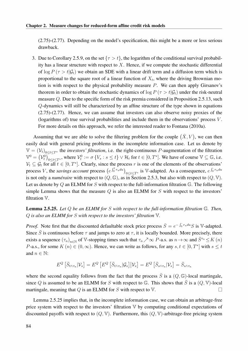
Chapter 2. Measure changes for reduced-form affine credit risk models
(2.75)-(2.77). Depending on the model’s specification, this might be a more or less seriousdrawback.
3. Due to Corollary 2.5.9, on the set τ > t, the logarithm of the conditional survival probabil-ity has a linear structure with respect to X . Hence, if we compute the stochastic differentialof logP (τ > t|Gt) we obtain an SDE with a linear drift term and a diffusion term which isproportional to the square root of a linear function of Xt, where the driving Brownian mo-tion is with respect to the physical probability measure P . We can then apply Girsanov’stheorem in order to obtain the stochastic dynamics of logP (τ > t|Gt) under the risk-neutralmeasureQ. Due to the specific form of the risk premia considered in Proposition 2.5.13, suchQ-dynamics will still be characterized by an affine structure of the type shown in equations(2.75)-(2.77). Hence, we can assume that investors can also observe noisy proxies of the(logarithms of) true survival probabilities and include them in the observations’ process V .For more details on this approach, we refer the interested reader to Fontana (2010a).
Assuming that we are able to solve the filtering problem for the couple(X, V
), we can then
easily deal with general pricing problems in the incomplete information case. Let us denote byV = (Vt)0≤t≤T ∗ the investors’ filtration, i.e. the right-continuous P -augmentation of the filtrationV0 =
(V0t
)0≤t≤T ∗ , where V0
t := σ Vs : s ≤ t ∨Ht for t ∈ [0, T ∗]. We have of course V ⊆ G, i.e.Vt ⊆ Gt for all t ∈ [0, T ∗]. Clearly, since the process r is one of the elements of the observations’process V , the savings account process
(e∫ t0 rudu
)0≤t≤T ∗ is V-adapted. As a consequence, e
∫ ·0 rudu
is not only a numéraire with respect to (Q,G), as in Section 2.5.3, but also with respect to (Q,V).Let us denote by Q an ELMM for S with respect to the full-information filtration G. The followingsimple Lemma shows that the measure Q is also an ELMM for S with respect to the investors’filtration V.
Lemma 2.5.25. Let Q be an ELMM for S with respect to the full-information filtration G. Then,Q is also an ELMM for S with respect to the investors’ filtration V.
Proof. Note first that the discounted defaultable stock price process S = e−∫ ·0 ruduS is V-adapted.
Since S is continuous before τ and jumps to zero at τ , it is locally bounded. More precisely, thereexists a sequence (τn)n∈N of V-stopping times such that τn∞ P -a.s. as n→∞ and Sτn≤K (n)
P -a.s., for some K (n) ∈ (0,∞). Hence, we can write as follows, for any s, t ∈ [0, T ∗] with s ≤ t
and n ∈ N:
EQ[St∧τn|Vs
]= EQ
[EQ[St∧τn|Gs
]∣∣Vs] = EQ[Ss∧τn|Vs
]= Ss∧τn
where the second equality follows from the fact that the process S is a (Q,G)-local martingale,since Q is assumed to be an ELMM for S with respect to G. This shows that S is a (Q,V)-localmartingale, meaning that Q is an ELMM for S with respect to V.
Lemma 2.5.25 implies that, in the incomplete information case, we can obtain an arbitrage-freeprice system with respect to the investors’ filtration V by computing conditional expectations ofdiscounted payoffs with respect to (Q,V). Furthermore, this (Q,V)-arbitrage-free pricing system
84

2.5 Application: a multifactor equity/credit risk model with stochastic volatility
is linked in an intuitive way to the original full information (Q,G)-arbitrage-free pricing system15.To see this, for t, T ∈ [0, T ∗] with t ≤ T , let us denote by Π (t, T ;F ) the (Q,G)-arbitrage-freeprice at time t of an integrable contingent claim F with maturity T . We have then16:
Π (t, T ;F ) := EQ[e−
∫ Tt rudu F
∣∣Vt] = EQ[EQ[e−
∫ Tt rudu F
∣∣Gt]∣∣∣Vt] = EQ [Π (t, T ;F ) |Vt](2.78)
where we have denoted by Π (t, T ;F ) the (Q,V)-arbitrage-free price at time t of the contingentclaim F .
The following Proposition deals with the general problem of computing the (Q,V)-arbitrage-free price of a credit-risky derivative which pays on the set τ > t a random amount F (XT ) atthe maturity T , for F : Rd+2 → R+.
Proposition 2.5.26. Let t, T ∈ [0, T ∗] with t ≤ T and F : Rd+2 → R+. Then the (Q,V)-arbitrage-free price at time t of the random payoff F (XT ) at maturity T on the event τ > T,with zero recovery in the case of default, is given by the following expression:
EQ[e−
∫ Tt ruduF (XT ) (1−HT )
∣∣∣Vt] = Πdf (t, T )EQT [F (XT ) |Vt] (2.79)
where the measure QT Q on (Ω,G) is defined as follows:
dQT
dQ:=
e−∫ T0 rudu (1−HT )
EQ[e−
∫ T0 rudu (1−HT )
]and Πdf (t, T ) denotes the (Q,V)-arbitrage-free price at time t of a 0-coupon 0-recovery default-able bond with maturity T , explicitly given as follows:
Πdf (t, T ) = (1−Ht) eΦQ(T−t,0) EQ
[eΨQ(T−t,0)′Xt
∣∣Vt] (2.80)
Furthermore, the Vt-conditional characteristic function of XT with respect to the measure QT isgiven as follows on the set τ > t, for all u ∈ iRd+2:
ϕTt (u) := EQT[eu′XT |Vt
]=eΦQ(T−t,u) EQ
[eΨQ(T−t,u)′Xt
∣∣Vt]eΦQ(T−t,0)EQ
[eΨQ(T−t,0)′Xt
∣∣Vt] (2.81)
where the functions ΦQ : [0, T ∗] × Cd+2 → C and ΨQ : [0, T ∗] × Cd+2 → Cd+2 are the uniquesolutions to the system of Riccati ODEs (2.60).
Proof. Equation (2.79) follows directly by using the definition of the measure QT together withBayes’ rule and equation (2.78), here applied to the arbitrage-free price of a 0-coupon 0-recoverydefaultable bond with maturity T . To prove equation (2.80) it suffices to combine (2.78) with part(b) of Corollary 2.5.19. Hence, it remains to show that the Vt-conditional characteristic function of
15We refer the reader to Gombani et al. (2007) for a more detailed analysis of the consistency of arbitrage-freepricing systems with respect to different filtrations.
16An analogous result can be found in Lemma 3.1 of Fontana & Runggaldier (2010).
85

Chapter 2. Measure changes for reduced-form affine credit risk models
the random vector XT under the measure QT can be expressed as in (2.81). On the set τ > t =
Ht = 0, this can be shown as follows, for any u ∈ iRd+2:
EQT[eu′XT |Vt
]=EQ[e−
∫ Tt rudu (1−HT ) eu
′XT∣∣Vt]
EQ[e−
∫ Tt rudu (1−HT )
∣∣Vt]=EQ[EQ[e−
∫ Tt rudu (1−HT ) eu
′XT∣∣Gt]∣∣Vt]
EQ[EQ[e−
∫ Tt rudu (1−HT )
∣∣Gt]∣∣Vt]=EQ[EQ[e−
∫ Tt (ru+λQu )du∣∣Ft]EQT
[eu′XT |Ft
]∣∣Vt]eΦQ(T−t,0)EQ
[eΨQ(T−t,0)′Xt
∣∣Vt]=eΦQ(T−t,u) EQ
[eΨQ(T−t,u)′Xt
∣∣Vt]eΦQ(T−t,0) EQ
[eΨQ(T−t,0)′Xt
∣∣Vt]where the first equality follows from the definition of the measure QT , the third equality (for the nu-merator) is due to Proposition 2.5.15 applied to the function F (x) = eu
′x and (for the denominator)to part (b) of Corollary 2.5.19 and the fourth equality uses Proposition 2.5.18.
Remark 2.5.27.
1. As can be seen from Proposition 2.5.26 and (2.81), the key ingredient for the computationof arbitrage-free prices at time t with respect to the investors’ filtration V turns out to be theVt-conditional characteristic function of the random vectorXt under the risk-neutral measureQ. This can be easily computed as soon as we manage to solve the filtering problem for thecouple
(X, V
)under the measure Q.
2. It is interesting to observe that the probability measure QT introduced in Proposition 2.5.26is similar to the T -forward survival risk-neutral measure QT introduced at the beginning ofSection 2.5.3. The only difference is that the density dQT
dQinvolves the default indicator term
(1−HT ), which may be equal to 0 in the case of default, unlike the term e−∫ Tt λQu du. As a
consequence, the measure QT is absolutely continuous with respect toQ but is not equivalentto Q. However, this has no implications for the arbitrage-free properties of the model, sincewe only use the measure QT as a computational tool.
3. Clearly, by following the arguments used in the proof of Proposition 2.5.16, one can extendProposition 2.5.26 to the arbitrage-free valuation of recovery payments with respect to theinvestors’ filtration V.
2.5.5 Connections to the literature
We give here a very brief overview of the related literature on the joint modeling of equity and creditrisk, which has been the subject of several recent papers. In particular, in Campi et al. (2009), Carr
86

2.6 Conclusions and further developments
& Linetsky (2006) and Carr & Madan (2010) the authors consider local volatility models (morespecifically, Campi et al. (2009) and Carr & Linetsky (2006) work with a CEV process) for thestock price process and introduce a random default time modeled as the first jump time of a Poissonprocess with stochastic intensity, the latter being given by a deterministic function of the pre-defaultstock price. Moving from a local volatility to a stochastic volatility approach, Carr & Schoutens(2008) and Carr & Wu (2010) consider the classical stochastic volatility model of Heston (1993)with the inclusion of an unpredictable jump to default. In the present Chapter, we embed thesemodels into a rather general class of multivariate affine diffusion models.
The very recent paper by Cheridito & Wugalter (2011) is rather close to our framework. Indeed,the authors jointly model the stock price process, its volatility and a vector of stochastic factors viaa multivariate affine process, allowing also for jumps in the factors’ dynamics, and then proceed tothe analysis of pricing and hedging problems for several typical payoff structures. However, theydo only consider the model under an a priori chosen risk-neutral probability measure, while themajor focus of this Chapter consists in studying the model under both the physical and the risk-neutral probability measure, ensuring that the structure of the model is preserved after the changeof measure. Indeed, the common approach in the literature surveyed so far is to formulate a modelwith respect to an exogenously fixed risk-neutral probability measure, the only exception being thepapers by Campi et al. (2009) and, to a lesser extent, Carr & Wu (2010). Even in the last twopapers, the authors adopt very particular specifications of the risk premium process and, therefore,our more general results could be of interest.
Concerning the financial interpretation as risk premia of the processes θ and γ appearing indensity process of a risk-neutral probability measure, we refer the interested reader to El Karoui &Martellini (2001), Driessen (2005), Jarrow et al. (2005), Section 9.3 of McNeil et al. (2005) andGiesecke & Goldberg (2008). In particular, Driessen (2005) points out the importance of explicitlydistinguishing between the risk of credit spread changes, if no default occurs, from the risk of thedefault event itself. A positive jump-type risk premium indicates that not enough corporate bonds(or analogous default-sensitive products) are traded in order to fully diversify the default jump risk.Furthermore, if one does not allow for a jump-type risk premium, one then incurs into the risk ofmisspecifying the model, thus leading to an inaccurate fit of the observed default rates. In Giesecke& Goldberg (2008), the authors propose a different interpretation of the risk premium process γ interms of a transparency premium required by investors to compensate for their imperfect knowledgeof the threshold which triggers the default event in the context of a structural model.
2.6 Conclusions and further developments
In this Chapter, we have studied the effects of (locally) equivalent changes of measure on reduced-form credit risk models, where the default intensity is driven by a multivariate diffusion affineprocess. In particular, we have established necessary and sufficient conditions for the preserva-tion of the affine structure of the model under a locally equivalent change of measure. As anapplication, we have considered a defaultable extension of the popular Heston (1993) stochastic
87
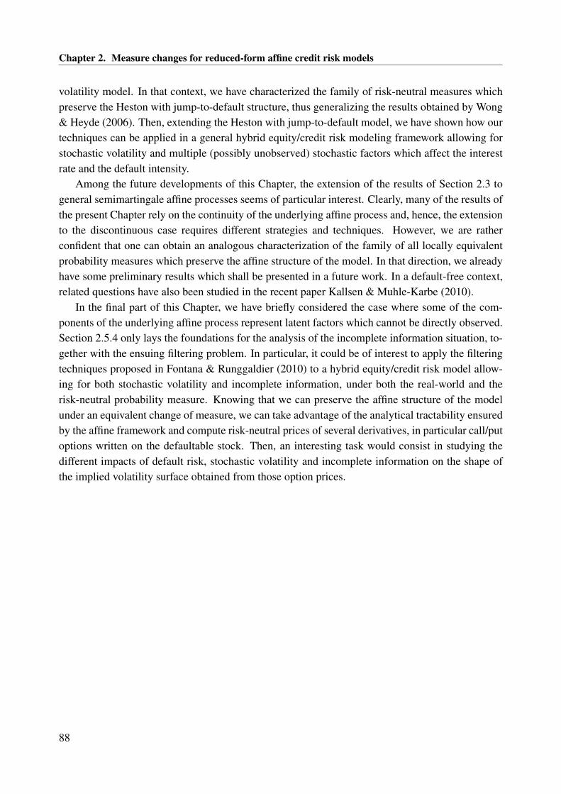
Chapter 2. Measure changes for reduced-form affine credit risk models
volatility model. In that context, we have characterized the family of risk-neutral measures whichpreserve the Heston with jump-to-default structure, thus generalizing the results obtained by Wong& Heyde (2006). Then, extending the Heston with jump-to-default model, we have shown how ourtechniques can be applied in a general hybrid equity/credit risk modeling framework allowing forstochastic volatility and multiple (possibly unobserved) stochastic factors which affect the interestrate and the default intensity.
Among the future developments of this Chapter, the extension of the results of Section 2.3 togeneral semimartingale affine processes seems of particular interest. Clearly, many of the results ofthe present Chapter rely on the continuity of the underlying affine process and, hence, the extensionto the discontinuous case requires different strategies and techniques. However, we are ratherconfident that one can obtain an analogous characterization of the family of all locally equivalentprobability measures which preserve the affine structure of the model. In that direction, we alreadyhave some preliminary results which shall be presented in a future work. In a default-free context,related questions have also been studied in the recent paper Kallsen & Muhle-Karbe (2010).
In the final part of this Chapter, we have briefly considered the case where some of the com-ponents of the underlying affine process represent latent factors which cannot be directly observed.Section 2.5.4 only lays the foundations for the analysis of the incomplete information situation, to-gether with the ensuing filtering problem. In particular, it could be of interest to apply the filteringtechniques proposed in Fontana & Runggaldier (2010) to a hybrid equity/credit risk model allow-ing for both stochastic volatility and incomplete information, under both the real-world and therisk-neutral probability measure. Knowing that we can preserve the affine structure of the modelunder an equivalent change of measure, we can take advantage of the analytical tractability ensuredby the affine framework and compute risk-neutral prices of several derivatives, in particular call/putoptions written on the defaultable stock. Then, an interesting task would consist in studying thedifferent impacts of default risk, stochastic volatility and incomplete information on the shape ofthe implied volatility surface obtained from those option prices.
88
Chapter 3
Diffusion-based models for financialmarkets without martingale measures
3.1 Introduction
The concepts of Equivalent (Local) Martingale Measure (E(L)MM), no-arbitrage and risk-neutralpricing can be rightfully considered as the cornerstones of modern mathematical finance. It seemsto be almost folklore that such concepts can be regarded as mutually equivalent. In fact, mostpractical applications in quantitative finance are directly formulated under suitable assumptionswhich ensure that those concepts are indeed equivalent.
In recent years, maybe due to the dramatic turbulences raging over financial markets, an increas-ing attention has been paid to models that allow for financial market anomalies. More specifically,several authors have studied market models where stock price bubbles may occur: see e.g. Cox& Hobson (2005), Heston et al. (2007), Hulley (2010), Jarrow et al. (2007), Jarrow et al. (2010).It has been shown that bubble phenomena are consistent with the classical no-arbitrage theorybased on the notion of No Free Lunch with Vanishing Risk (NFLVR), as developed in Delbaen& Schachermayer (1994) and Delbaen & Schachermayer (2006). However, in the presence of abubble, discounted prices of risky assets follow, under a risk-neutral measure, a strict local martin-gale, i.e. a local martingale which is not a true martingale. This fact already implies that severalwell-known and classical results (for instance put-call parity, see e.g. Cox & Hobson (2005)) ofmathematical finance do not hold anymore and must be modified accordingly.
A decisive step towards enlarging the scope of financial models has been represented by thestudy of models which do not fit at all into the classical no-arbitrage theory based on (NFLVR).Indeed, several authors (see e.g. Christensen & Larsen (2007), Delbaen & Schachermayer (1995a),Hulley (2010), Karatzas & Kardaras (2007), Loewenstein & Willard (2000)) have studied instanceswhere an ELMM may fail to exist. More specifically, financial models that do not admit an ELMMappear in the context of Stochastic Portfolio Theory (see Fernholz & Karatzas (2009) for a recentoverview) and in the Benchmark Approach (see the monograph Platen & Heath (2006) for a detailedaccount). In the absence of a well-defined ELMM, many of the usual results of mathematical
89

Chapter 3. Diffusion-based models for financial markets without martingale measures
finance seem to break down and one is led to ask whether there is still a meaningful way to proceedin order to solve the crucial problems of portfolio optimisation and contingent claim valuation. Itis then a remarkable result that a satisfactory theory can be developed even in the absence of anELMM, especially in the case of a complete financial market model, as we are going to illustrate.
The present Chapter aims at carefully analysing a general class of diffusion-based financialmodels, without relying on the existence of an ELMM. More specifically, we discuss several no-tions of no-arbitrage that are weaker than the traditional (NFLVR) condition and we study necessaryand sufficient conditions for their validity. We show that the financial market may still be viable,in a sense to be made precise, even in the absence of an ELMM. In particular, it turns out that theviability of the financial market is fundamentally linked to a square-integrability property of themarket price of risk process. Some of the results that we are going to present have already beenobtained, also in more general settings (see e.g. Christensen & Larsen (2007), Hulley & Schweizer(2010), Karatzas & Kardaras (2007), Kardaras (2010b)). However, by exploiting the Itô-processstructure of our model, we are able to provide simple and transparent proofs, highlighting the keyideas behind the general theory. We also discuss the connections to the Growth-Optimal Portfolio(GOP), which is shown to be the unique portfolio possessing the numéraire property. In similardiffusion-based settings, related works that study the question of market viability in the absenceof an ELMM include Fernholz & Karatzas (2009), Galesso & Runggaldier (2010), Heston et al.(2007), Loewenstein & Willard (2000), Londono (2004), Platen (2002) and Runggaldier (2003).
Besides studying the question of market viability, a major focus of this Chapter is on the valua-tion and hedging of contingent claims in the absence of an ELMM. In particular, we argue that theconcept of market completeness, namely the capability to replicate every contingent claim, must bekept distinct from the existence of an ELMM. Indeed, we prove that the financial market may beviable and complete regardless of the existence of an ELMM. We then show that, in the context ofa complete financial market, there is a unique natural candidate for the price of an arbitrary contin-gent claim, given by its GOP-discounted expected value under the original (real-world) probabilitymeasure. To this effect, we revisit some ideas originally appeared in the context of the BenchmarkApproach, providing more careful proofs and extending some previous results.
The present Chapter is strongly linked to Chapter 4. In fact, on the one hand, many of theresults of the present Chapter can be recovered by specializing the more general results of Chapter4 to the case of an Itô-process-based model for a financial market. On the other hand, since theresults of Chapter 4 are formulated in general and abstract terms, the present Chapter can alsoserve as an illustration of the concepts and of the main results contained in Chapter 4, avoidingsome of the technicalities which arise in the more general context by restricting our attention to adiffusion-based financial market model.
The present Chapter is structured as follows. Section 3.2 introduces the general setting, whichconsists of a class of Itô-process models satisfying minimal technical conditions. We introduce abasic standing Assumption and we carefully describe the set of admissible trading strategies. Thequestion of whether (properly defined) arbitrage opportunities do exist or not is dealt with in Section3.3. In particular, we explore the notions of increasing profit and arbitrage of the first kind, givingnecessary and sufficient conditions for their absence from the financial market. In turn, this lead us
90

3.2 The general setting
to introduce the concept of martingale deflators, which can be regarded as weaker counterparts tothe traditional martingale measures. Section 3.4 proves the existence of an unique Growth-Optimalstrategy, which admits an explicit characterization and also generates the numéraire portfolio. Inturn, the latter is shown to be the reciprocal of a martingale deflator, thus linking the numéraireportfolio to the no-arbitrage criteria discussed in Section 3.3. Section 3.5 starts with the hedgingand valuation of contingent claims, showing that the financial market may be complete even inthe absence of an ELMM. Section 3.6 deals with contingent claim valuation according to three al-ternative approaches: real-world pricing, upper-hedging pricing and utility indifference valuation.In the particular case of a complete market, we show that they yield the same valuation formula.Section 6 concludes by pointing out possible extensions and further developments.
3.2 The general setting
Let (Ω,F , P ) be a complete probability space. For a fixed time horizon T ∈ (0,∞), let F =
(Ft)0≤t≤T be a filtration on (Ω,F , P ) satisfying the usual conditions of right-continuity and com-pleteness. Let W = (Wt)0≤t≤T be an Rd-valued Brownian motion on the filtered probability space(Ω,F ,F, P ). To allow for greater generality we do not assume from the beginning that F = FW ,meaning that the filtration F may be strictly larger than the P -augmented Brownian filtration FW .Also, the initial σ-field F0 may be strictly larger than the trivial σ-field.
We consider a financial market composed of N + 1 securities Si, for i = 0, 1, . . . , N , withN ≤ d. As usual, we let S0 represent a locally riskless asset, which we name savings account, andwe define the process S0 = (S0
t )0≤t≤T as follows:
S0t := exp
(∫ t
0
ru du
)for t ∈ [0, T ] (3.1)
where the interest rate process r = (rt)0≤t≤T is a real-valued progressively measurable processsuch that
∫ T0|rt| dt < ∞ P -a.s. The remaining assets Si, for i = 1, . . . , N , are supposed to be
risky assets. For i = 1, . . . , N , the process Si = (Sit)0≤t≤T is given by the solution to the followingSDE:
dSit = Sit µit dt+
d∑j=1
Sit σi,jt dW j
t Si0 = si (3.2)
where:
(i) si ∈ (0,∞) for all i = 1, . . . , N ;
(ii) µ = (µt)0≤t≤T is an RN -valued progressively measurable process with µt =(µ1t , . . . , µ
Nt
)′and satisfying
∫ T0‖µt‖ dt <∞ P -a.s.;
(iii) σ = (σt)0≤t≤T is an RN×d-valued progressively measurable process with σt =σi,jti=1,...,Nj=1,...,d
and satisfying∑N
i=1
∑dj=1
∫ T0
(σi,jt)2dt <∞ P -a.s.
91

Chapter 3. Diffusion-based models for financial markets without martingale measures
The SDE (3.2) admits the following explicit solution, for every i = 1, . . . , N and t ∈ [0, T ]:
Sit = si exp
(∫ t
0
(µiu −
1
2
d∑j=1
(σi,ju)2)du+
d∑j=1
∫ t
0
σi,ju dW ju
)(3.3)
Note that conditions (ii)-(iii) above represent minimal conditions in order to have a meaningfuldefinition of the ordinary and stochastic integrals appearing in (3.3). Apart from these technicalrequirements, we leave the stochastic processes µ and σ fully general. For i = 0, 1, . . . , N , wedenote by Si =
(Sit)
0≤t≤T the discounted price process of the i-th asset, defined as Sit := Sit/S0t
for t ∈ [0, T ].Let us now introduce the following standing Assumption, which we shall always assume to be
satisfied without any further mention.
Assumption 3.2.1. For all t ∈ [0, T ], the (N × d)-matrix σt has P -a.s. full rank.
Remark 3.2.2. From a financial perspective, Assumption 3.2.1 means that the financial marketdoes not contain redundant assets, i.e. there does not exist a non-trivial linear combination of(S1, . . . , SN
)that is locally riskless, in the sense that its dynamics are not affected by the Brownian
motion W . However, we want to point out that Assumption 3.2.1 is only used in the following forproving uniqueness properties of trading strategies and, hence, could also be relaxed.
In order to rigorously describe the activity of trading in the financial market, we now introducethe concepts of trading strategy and discounted portfolio process. In the following Definition weonly consider self-financing trading strategies which generate positive portfolio processes.
Definition 3.2.3.
(a) An RN -valued progressively measurable process π = (πt)0≤t≤T is an admissible tradingstrategy if
∫ T0‖σ′t πt‖
2 dt < ∞ P -a.s. and∫ T
0|π′t (µt − rt1)| dt < ∞ P -a.s., where 1 :=
(1, . . . , 1)′ ∈ RN . We denote by A the set of all admissible trading strategies.
(b) For any (v, π) ∈ R+ ×A, the associated discounted portfolio process V v,π =(V v,πt
)0≤t≤T
is defined by:
V v,πt := v E
(N∑i=1
∫πidSi
Si
)t
= v exp
(∫ t
0
π′u (µu − ru1) du− 1
2
∫ t
0
‖σ′u πu‖2du+
∫ t
0
π′u σu dWu
) (3.4)
for all t ∈ [0, T ], where E (·) denotes the stochastic exponential.
The integrability conditions in part (a) of Definition 3.2.3 ensure that both the ordinary andthe stochastic integrals appearing in (3.4) are well-defined. For all i = 1, . . . , N and t ∈ [0, T ],πit represents the proportion of wealth invested in the i-th risky asset Si at time t. Consequently,1 − π′t1 represents the proportion of wealth invested in the savings account S0 at time t. Note
92

3.3 No-arbitrage conditions and the market price of risk
that part (b) of Definition 3.2.3 corresponds to requiring the trading strategy π to be self-financing.Observe that Definition 3.2.3 implies that, for any (v, π) ∈ R+ × A, we have V v,π
t = v V 1,πt , for
all t ∈ [0, T ]. Due to this scaling property, we shall often let v = 1 without loss of generality,denoting V π := V 1,π for any π ∈ A. By definition, the discounted portfolio process V π satisfiesthe following dynamics:
dV πt = V π
t
N∑i=1
πitdSitSit
= V πt π′t (µt − rt1) dt+ V π
t π′t σt dWt (3.5)
Remark 3.2.4. The fact that admissible portfolio processes are uniformly bounded from below byzero excludes pathological doubling strategies (see e.g. Karatzas & Shreve (1998), Section 1.1.2).Moreover, an economic motivation for focusing on positive portfolios only is given by the fact thatmarket participants have limited liability and, therefore, are not allowed to trade anymore if theirtotal tradeable wealth reaches zero. See also Section 2 of Christensen & Larsen (2007), Section 6of Platen (2009) and Section 10.3 of Platen & Heath (2006) for an amplification of this point.
3.3 No-arbitrage conditions and the market price of risk
In order to ensure that the model introduced in the previous Section represents a viable finan-cial market, in a sense to be made precise (see Definition 3.3.9), we need to carefully answer thequestion of whether properly defined arbitrage opportunities are excluded. We start by giving thefollowing Definition.
Definition 3.3.1. A trading strategy π ∈ A is said to yield an increasing profit if the correspondingdiscounted portfolio process V π =
(V πt
)0≤t≤T satisfies the following two conditions:
(a) V π is P -a.s. increasing, in the sense that P(V πs ≤ V π
t for all s, t ∈ [0, T ] with s ≤ t)
= 1;
(b) P(V πT > 1
)> 0.
The notion of increasing profit represents the most glaring type of arbitrage opportunity and,hence, it is of immediate interest to know whether it is allowed or not in the financial market. As apreliminary, the following Lemma gives an equivalent characterization of the notion of increasingprofit. We denote by ` the Lebesgue measure on [0, T ].
Lemma 3.3.2. There exists an increasing profit if and only if there exists a trading strategy π ∈ Asatisfying the following two conditions:
(a) π′t σt = 0 P ⊗ `-a.e.;
(b) π′t (µt − rt1) 6= 0 on some subset of Ω× [0, T ] with positive P ⊗ `-measure.
Proof. Let π ∈ A be a trading strategy yielding an increasing profit. Due to Definition 3.3.1,the process V π is P -a.s. increasing, hence of finite variation. Equation (3.5) implies then that
93
Chapter 3. Diffusion-based models for financial markets without martingale measures
the continuous local martingale(∫ t
0V πu π′u σu dWu
)0≤t≤T
is also of finite variation. This fact in
turn implies that π′t σt = 0 P ⊗ `-a.e. (see e.g. Karatzas & Shreve (1991), Section 1.5). SinceP(V πT > 1
)> 0, we must have π′t (µt − rt1) 6= 0 on some subset of Ω × [0, T ] with positive
P ⊗ `-measure.Conversely, let π ∈ A be a trading strategy satisfying conditions (a)-(b). Define then the process
π = (πt)0≤t≤T as follows, for t ∈ [0, T ]:
πt := sign(π′t (µt − rt1)
)πt
It is clear that π ∈ A and π′t σt = 0 P ⊗ `-a.e. and hence, due to (3.4), for all t ∈ [0, T ]:
V πt = exp
(∫ t
0
π′u (µu − ru1) du
)Furthermore, we have that π′t (µt − rt1) ≥ 0, with strict inequality holding on some subset ofΩ × [0, T ] with positive P ⊗ `-measure. This implies that the process V π =
(V πt
)0≤t≤T is P -a.s.
increasing and satisfies P(V πT > 1
)> 0, meaning that π yields an increasing profit.
The following Proposition gives a necessary and sufficient condition in order to exclude theexistence of increasing profits (compare also with Theorem 4.3.2 in Chapter 4).
Proposition 3.3.3. There are no increasing profits if and only if there exists an Rd-valued progres-sively measurable process γ = (γt)0≤t≤T such that the following condition holds:
µt − rt1 = σtγt P ⊗ `-a.e. (3.6)
Proof. Suppose there exists an Rd-valued progressively measurable process γ = (γt)0≤t≤T suchthat (3.6) is satisfied and let π ∈ A be such that π′t σt = 0 P ⊗ `-a.e. Then we have:
π′t (µt − rt1) = π′t σtγt = 0 P ⊗ `-a.e.
meaning that there cannot exist a trading strategy π ∈ A satisfying conditions (a)-(b) of Lemma3.3.2. Due to the equivalence result of Lemma 3.3.2, this implies that there are no increasing profits.
Conversely, suppose that there exists no trading strategy in A yielding an increasing profit. Letus first introduce the following linear spaces, for every t ∈ [0, T ]:
R (σt) :=σty : y ∈ Rd
K (σ′t) :=
y ∈ RN : σ′ty = 0
Denote by ΠK(σ′t)
the orthogonal projection on K (σ′t). As in Lemma 1.4.6 of Karatzas & Shreve(1998), we define the process p = (pt)0≤t≤T by:
pt := ΠK(σ′t)(µt − rt1)
Define then the process π = (πt)0≤t≤T by:
πt :=
pt‖pt‖ if pt 6= 0,
0 if pt = 0.
94

3.3 No-arbitrage conditions and the market price of risk
Since the processes µ and r are progressively measurable, Corollary 1.4.5 of Karatzas & Shreve(1998) ensures that π is progressively measurable. Clearly, we have then π ∈ A and, by definition,π satisfies condition (a) of Lemma 3.3.2. Since there are no increasing profits, Lemma 3.3.2 impliesthat the following identity holds P ⊗ `-a.e.:
‖pt‖ =p′t‖pt‖
(µt − rt1)1pt 6=0 = π′t (µt − rt1)1pt 6=0 = 0 (3.7)
where the first equality uses the fact that µt − rt1 − pt ∈ K⊥ (σ′t), for all t ∈ [0, T ], with thesuperscript⊥ denoting the orthogonal complement. From (3.7) we have pt = 0 P⊗`-a.e., meaningthat µt − rt1 ∈ K⊥ (σ′t) = R (σt) P ⊗ `-a.e. This amounts to saying that we have:
µt − rt1 = σtγt P ⊗ `-a.e.
for some γt ∈ Rd. Taking care of the measurability issues, it can be shown that we can takeγ = (γt)0≤t≤T as a progressively measurable process (compare Karatzas & Shreve (1998), proof ofTheorem 1.4.2).
Let us now introduce one of the crucial objects in our analysis: the market price of risk process.
Definition 3.3.4. The Rd-valued progressively measurable market price of risk process θ = (θ)0≤t≤Tis defined as follows, for t ∈ [0, T ]:
θt := σ′t (σt σ′t)−1
(µt − rt1)
The standing Assumption 3.2.1 ensures that the market price of risk process θ is well-defined1.From a financial perspective, θt measures the excess return (µt − rt1) of the risky assets (withrespect to the savings account) in terms of their volatility.
Remark 3.3.5 (Absence of increasing profits). Note that, by definition, the market price of riskprocess θ satisfies condition (3.6). Proposition 3.3.3 then implies that, under the standing Assump-tion 3.2.1, there are no increasing profits. Note however that θ may not be the unique processsatisfying condition (3.6).
Let us now introduce the following integrability condition on the market price of risk process.
Assumption 3.3.6. The market price of risk process θ = (θt)0≤t≤T belongs to L2loc (W ), meaning
that∫ T
0‖θt‖2 dt <∞ P -a.s.
Remark 3.3.7. Let γ = (γt)0≤t≤T be an Rd-valued progressively measurable process satisfy-ing condition (3.6). Using the notation R (σ′t) =
σ′t x : x ∈ RN
and R⊥ (σ′t) = K (σt) =
x ∈ Rd : σt x = 0
, we have the orthogonal decomposition γt = ΠR(σ′t)(γt) + ΠK(σt) (γt), for
t ∈ [0, T ]. Under Assumption 3.2.1, elementary linear algebra shows that:
ΠR(σ′t)(γt) = σ′t (σtσ
′t)−1σtγt = σ′t (σtσ
′t)−1
(µt − rt1) = θt
1It is worth pointing out that, if Assumption 3.2.1 does not hold, then the market price of risk process θ can still bedefined by replacing σ′t (σt σ
′t)−1 with the Moore-Penrose pseudoinverse of the matrix σt.
95

Chapter 3. Diffusion-based models for financial markets without martingale measures
thus giving ‖γt‖ = ‖θt‖ +∥∥ΠK(σt) (γt)
∥∥ ≥ ‖θt‖, for all t ∈ [0, T ]. This implies that, as soonas there exists some Rd-valued progressively measurable process γ satisfying (3.6) and such thatγ ∈ L2
loc (W ), then the market price of risk process θ satisfies Assumption 3.3.6.
The key relation between Assumption 3.3.6 and no-arbitrage was first discovered in Delbaen &Schachermayer (1995b) and Levental & Skorohod (1995) and will play a crucial role in derivingmany of our results. We now introduce a fundamental local martingale associated to the marketprice of risk process θ. Let us define the process Z =
(Zt)
0≤t≤T as follows, for t ∈ [0, T ]:
Zt := E(−∫θ′dW
)t
= exp
(−
d∑j=1
∫ t
0
θju dWju −
1
2
d∑j=1
∫ t
0
(θju)2du
)(3.8)
Note that Assumption 3.3.6 ensures that the stochastic integral∫θ′dW is well-defined as a contin-
uous local martingale. It is well-known that Z =(Zt)
0≤t≤T is a strictly positive continuous local
martingale with Z0 = 1. Hence, due to Fatou’s Lemma, the process Z is also a supermartingale(see e.g. Karatzas & Shreve (1991), Problem 1.5.19) and we have E
[ZT]≤ E
[Z0
]= 1. It is
easy to show that the process Z is a true martingale, and not only a local martingale, if and only ifE[ZT]
= E[Z0
]= 1. However, it may happen that the process Z is a strict local martingale, i.e.
a local martingale which is not a true martingale. In any case, the following Proposition shows thebasic property of the process Z.
Proposition 3.3.8. Suppose that Assumption 3.3.6 holds and let Z =(Zt)
0≤t≤T be defined as in(3.8). Then the following hold:
(a) for all i = 1, . . . , N , the process Z Si =(Zt S
it
)0≤t≤T is a local martingale;
(b) for any trading strategy π ∈ A the process Z V π =(Zt V
πt
)0≤t≤T is a local martingale.
Proof. For any i = 1, . . . , N , part (a) follows from part (b) by taking π ∈ A with πi ≡ 1 andπj ≡ 0 for j 6= i. Hence, it suffices to prove part (b). Recalling equation (3.5), an application ofthe Itô product rule gives:
d(Zt V
πt
)= V π
t dZt + Zt dVπt + d〈V π, Z〉t
= −V πt Zt θ
′t dWt + Zt V
πt π′t (µt − rt1) dt+ Zt V
πt π′t σt dWt − Zt V π
t π′t σt θt dt
= Zt Vπt (π′t σt − θ′t) dWt
(3.9)Since σ′π ∈ L2
loc (W ) and θ ∈ L2loc (W ), this shows the local martingale property of Z V π.
Under the standing Assumption 3.2.1, we have seen that the diffusion-based financial marketdescribed in Section 3.2 does not allow for increasing profits (see Remark 3.3.5). However, the con-cept of increasing profit represents an almost pathological notion of arbitrage opportunity. Hence,we would like to known whether weaker and more economically meaningful types of arbitrageopportunities can exist. To this effect, let us give the following Definition, adapted from Kardaras(2010b).
96

3.3 No-arbitrage conditions and the market price of risk
Definition 3.3.9. An F-measurable non-negative random variable ξ is called an arbitrage of thefirst kind if P (ξ > 0) > 0 and, for all v ∈ (0,∞), there exists a trading strategy πv ∈ A such thatV v,πv
T ≥ ξ P -a.s. We say that the financial market is viable if there are no arbitrages of the firstkind.
The following Proposition shows that the existence of an increasing profit implies the existenceof an arbitrage of the first kind. Due to the Itô-process framework considered in this Chapter, weare able to provide a simple proof (in a more general context, see also Section 4.3.3).
Proposition 3.3.10. Let π ∈ A be a trading strategy yielding an increasing profit. Then there existsan arbitrage of the first kind.
Proof. Let π ∈ A yield an increasing profit and define ξ := V πT − 1. Due to Definition 3.3.1, we
have P (ξ ≥ 0) = 1 and P (ξ > 0) > 0. Then, for any v ∈ [1,∞), we have V v,πT = vV π
T > v ξ ≥ ξ
P -a.s. For any v ∈ (0, 1), let us define πvt := − log(v)+log(1−v)v
πt. Clearly, for any v ∈ (0, 1), theprocess πv = (πvt )0≤t≤T satisfies πv ∈ A and, due to Lemma 3.3.2, (πvt )
′ σt = 0 P ⊗ `-a.e. Wehave then:
V v,πv
T = v exp
(∫ T
0
(πvt )′ (µt − rt1) dt
)= v
(V πT
)− log(v)+log(1−v)v > V π
T − 1 = ξ P -a.s.
where the second equality follows from the elementary identity exp (αx) = (expx)α and the lastinequality follows since vx−
log(v)+log(1−v)v > x− 1 for x ≥ 1 and for every v ∈ (0, 1). We have thus
shown that, for every v ∈ (0,∞), there exists a trading strategy πv ∈ A such that V v,πv
T ≥ ξ P -a.s.,meaning that the random variable ξ is an arbitrage of the first kind.
We now proceed with the question of whether arbitrages of the first kind are allowed in ourfinancial market model. To this effect, let us first give the following Definition (compare also withDefinition 4.3.11 in Chapter 4).
Definition 3.3.11. A real-valued non-negative adapted process D = (Dt)0≤t≤T with D0 = 1 andDT > 0 P -a.s. is said to be a martingale deflator if the product DV π =
(DtV
πt
)0≤t≤T is a local
martingale for every π ∈ A. We denote by D the set of all martingale deflators.
Remark 3.3.12. Let D ∈ D. Then, taking π ≡ 0, Definition 3.3.11 implies that D is a non-negative local martingale and hence, due to Fatou’s Lemma, also a supermartingale. Since DT > 0
P -a.s., the minimum principle for non-negative supermartingales (see e.g. Revuz & Yor (1999),Proposition II.3.4) implies that P
(Dt > 0 for all t ∈ [0, T ]
)= 1.
The following Proposition shows that the existence of a martingale deflator is a sufficient con-dition for the absence of arbitrages of the first kind.
Proposition 3.3.13. If D 6= ∅ then there cannot exist arbitrages of the first kind.
Proof. Let D ∈ D and suppose that there exists a random variable ξ yielding an arbitrage of thefirst kind. Then, for every n ∈ N, there exists a strategy πn ∈ A such that V 1/n,πn
T ≥ ξ P -a.s. For
97
Chapter 3. Diffusion-based models for financial markets without martingale measures
every n ∈ N, the process DV 1/n,πn =(DtV
1/n,πn
t
)0≤t≤T is a positive local martingale and, hence,
a supermartingale. So, for every n ∈ N:
E [DT ξ] ≤ E[DT V
1/n,πn
T
]≤ E
[D0V
1/n,πn
0
]=
1
n
Letting n→∞ gives E [DT ξ] = 0 and hence DT ξ = 0 P -a.s. Since, due to Definition 3.3.11, wehave DT > 0 P -a.s. this implies that ξ = 0 P -a.s., which contradicts the assumption that ξ is anarbitrage of the first kind.
It is worth pointing out that one can also prove a converse result to Proposition 3.3.13, showingthat if there are no arbitrages of the first kind then there exists at least one martingale deflator. Ina general semimartingale setting, this has been recently shown in Kardaras (2010b) (compare alsoHulley & Schweizer (2010) in the context of continuous path processes). Furthermore, Proposition1 of Kardaras (2010a) shows that the absence of arbitrages of the first kind is equivalent to thecondition of No Unbounded Profit with Bounded Risk (NUPBR), formally defined as the conditionthat the set
V πT : π ∈ A
be bounded in probability. By relying on these facts, we can state the
following Theorem, the second part of which follows from Proposition 4.19 of Karatzas & Kardaras(2007).
Theorem 3.3.14. The following are equivalent:
(a) D 6= ∅;
(b) there are no arbitrages of the first kind;
(c)V πT : π ∈ A
is bounded in probability, i.e. the condition (NUPBR) holds.
Moreover, for every concave and strictly increasing utility function U : [0,∞) → R, the utilityoptimisation problem of finding an element π∗ ∈ A such that
E[U(V π∗
T
)]= sup
π∈AE[U(V πT
)]either does not have a solution or has infinitely many solutions when any of the conditions (a)-(c)fails.
We want to remark that an analogous result has already been shown in Theorem 2 of Loewen-stein & Willard (2000) under the assumption of a complete financial market. In view of the secondpart of the above Theorem, the condition of absence of arbitrages of the first kind can be seen asthe minimal no-arbitrage condition in order to be able to meaningfully solve portfolio optimisationproblems. It is now straightforward to show that, as soon as Assumption 3.3.6 holds, the diffusion-based model introduced in Section 3.2 satisfies the equivalent conditions of Theorem 3.3.14. Infact, due to Proposition 3.3.8, the process Z defined in (3.8) is a martingale deflator for the finan-cial market
(S0, S1, . . . , SN
)as soon as Assumption 3.3.6 is satisfied. Conversely, if Assumption
3.3.6 fails to hold, then there cannot exist any martingale deflator (see Remark 3.3.7). In a moregeneral context, compare also with Theorem 4.3.23 in Chapter 4.
98
3.3 No-arbitrage conditions and the market price of risk
Corollary 3.3.15. The financial market(S0, S1, . . . , SN
)is viable, i.e. it does not admit arbitrages
of the first kind (see Definition 3.3.9), if and only if Assumption 3.3.6 holds.
We want to emphasise that, due to Theorem 3.3.14, the diffusion-based model introduced inSection 3.2 allows us to meaningfully consider portfolio optimisation problems as soon as As-sumption 3.3.6 holds. However, nothing guarantees that an Equivalent Local Martingale Measure(ELMM) exists, as shown in the following classical example, already considered in Delbaen &Schachermayer (1995a), Hulley (2010) and Karatzas & Kardaras (2007). Other instances of mod-els for which an ELMM does not exist arise in the context of diverse financial markets, see ChapterII of Fernholz & Karatzas (2009).
Example 3.3.16. Let us suppose that F = FW , where W is a standard Brownian motion (d = 1),and letN = 1. Assume that S0
t ≡ 1 for all t ∈ [0, T ] and that the real-valued process S = (St)0≤t≤Tis given as the solution to the following SDE:
dSt =1
Stdt+ dWt S0 = s ∈ (0,∞) (3.10)
It is well-known that the process S is a Bessel process of dimension three (see e.g. Revuz & Yor(1999), Section XI.1). So, St is P -a.s. strictly positive and finite for all t ∈ [0, T ]. Furthermore, themarket price of risk process θ is given by θt = σ−1
t µt = 1St
, for t ∈ [0, T ]. Since S is continuous,
we clearly have∫ T
0θ2t dt < ∞ P -a.s., meaning that Assumption 3.3.6 is satisfied. Hence, due to
Corollary 3.3.15, there are no arbitrages of the first kind.However, for this particular financial market model there exists no ELMM. We prove this claim
arguing by contradiction. Suppose that Q is an ELMM for S and denote by ZQ =(ZQt
)0≤t≤T
its density process. Then, due to the martingale representation theorem (see Karatzas & Shreve(1991), Theorem 3.4.15 and Problem 3.4.16), we can represent ZQ as follows:
ZQt = E
(−∫λ dW
)t
for t ∈ [0, T ]
where λ = (λt)0≤t≤T is a progressively measurable process such that∫ T
0λ2t dt < ∞ P -a.s. Due
to Girsanov Theorem, the process WQ =(WQt
)0≤t≤T defined by WQ
t := Wt +∫ t
0λu du, for
t ∈ [0, T ], is a Brownian motion under Q. Hence, the process S satisfies the following SDE underQ:
dSt =
(1
St− λt
)dt+ dWQ
t S0 = s (3.11)
Since Q is an ELMM for S, the SDE (3.11) must have a zero drift coefficient, i.e. it must beλt = 1
St= θt for all t ∈ [0, T ]. Then, a simple application of Itô’s formula gives:
ZQt = E
(−∫
1
SdW
)t
= exp
(−∫ t
0
1
SudWu −
1
2
∫ t
0
1
S2u
du
)=
1
St
However, since S is a Bessel process of dimension three, it is well-known that the process 1/S =
(1/St)0≤t≤T is a strict local martingale, i.e. it is a local martingale but not a true martingale (see e.g.Revuz & Yor (1999), Exercise XI.1.16). Clearly, this contradicts the fact that Q is a well-definedprobability measure, thus showing that there cannot exist an ELMM for S.
99

Chapter 3. Diffusion-based models for financial markets without martingale measures
As the above Example shows, Assumption 3.3.6 does not guarantee the existence of an ELMMfor the financial market
(S0, S1, . . . , SN
). It is well-known that, in the case of continuous-path
processes, the existence of an ELMM is equivalent to the no-arbitrage condition of No Free Lunchwith Vanishing Risk (NFLVR), see Delbaen & Schachermayer (1994) and Delbaen & Schacher-mayer (2006). Furthermore, (NFLVR) holds if and only if both (NUPBR) and (NA) hold (see Sec-tion 3 of Delbaen & Schachermayer (1994) and Proposition 4.2 of Karatzas & Kardaras (2007)),where, recalling that V π
0 = 1, the classical no-arbitrage condition (NA) precludes the existenceof a trading strategy π ∈ A such that P
(V πT ≥ 1
)= 1 and P
(V πT > 1
)> 0. This implies that,
even if Assumption 3.3.6 holds, the well-known no-arbitrage condition (NFLVR) may fail to hold.However, due to Theorem 3.3.14, the financial market may still be viable.
Remark 3.3.17 (On the martingale property of Z). It is important to note that Assumption 3.3.6does not suffice to ensure that Z is a true martingale. Well-known sufficient conditions for this tohold include the Novikov and Kazamaki criteria, see e.g. Revuz & Yor (1999), Section VIII.1. IfZ is a true martingale we have then E
[ZT]
= 1 and we can define a probability measure Q ∼ P
by letting dQdP
:= ZT . The martingale Z represents then the density process of Q with respect to
P , i.e. Zt = E[dQdP
∣∣Ft] P -a.s. for all t ∈ [0, T ]. Recall that a process M = (Mt)0≤t≤T is a
local Q-martingale if and only if the process ZM =(ZtMt
)0≤t≤T is a local P -martingale. Due
to Proposition 3.3.8-(a), this implies that if E[ZT]
= 1 then the process S :=(S1, . . . , SN
)′ is alocal Q-martingale or, in other words, the probability measure Q is an ELMM. Girsanov’s theoremimplies then that the process W =
(Wt
)0≤t≤T defined by Wt := Wt +
∫ t0θu du for t ∈ [0, T ] is a
Brownian motion under Q. Since the dynamics of S :=(S1, . . . , SN
)′ in (3.2) can be rewritten as:
dSt = diag (St)1 rt dt+ diag (St)σt(θt dt+ dWt
)S0 = s
the process S :=(S1, . . . , SN
)′ satisfies the following SDE under the measure Q:
dSt = diag(St)σt dWt S0 = s
We want to point out that the process Z =(Zt)
0≤t≤T represents the density process with respectto P of the minimal martingale measure, when the latter exists, see e.g. Hulley & Schweizer(2010). Again, we emphasise that in this Chapter we do not assume neither that E
[ZT]
= 1 northe existence of an ELMM.
We close this Section with a simple technical result which turns out to be useful in the following.
Lemma 3.3.18. Suppose that Assumption 3.3.6 holds. Then an RN -valued progressively measur-able process π = (πt)0≤t≤T belongs to A if and only if
∫ T0‖σ′t πt‖
2 dt <∞ P -a.s.
Proof. We only need to show that Assumption 3.3.6 and∫ T
0‖σ′t πt‖
2 dt <∞ P -a.s. together implythat
∫ T0|π′t (µt − rt1)| dt < ∞ P -a.s. This follows easily from the Cauchy-Schwarz inequality, in
fact:∫ T
0
|π′t (µt − rt1)| dt =
∫ T
0
|π′t σt θt| dt ≤(∫ T
0
‖σ′t πt‖2dt
) 12(∫ T
0
‖θt‖2 dt
) 12
<∞ P -a.s.
100
3.4 The growth-optimal portfolio and the numéraire portfolio
3.4 The growth-optimal portfolio and the numéraire portfolio
As we have seen in the last Section, the diffusion-based model introduced in Section 3.2 can rep-resent a viable financial market even if the traditional no-arbitrage condition (NFLVR) fails to holdor, equivalently, if an ELMM for
(S0, S1, . . . , SN
)fails to exist. Let us now consider an interesting
portfolio optimisation problem, namely the problem of maximising the growth rate, formally de-fined as follows (compare Fernholz & Karatzas (2009), Platen (2006) and Platen & Heath (2006),Section 10.2).
Definition 3.4.1. For a trading strategy π ∈ A the growth rate process gπ = (gπt )0≤t≤T is definedas the drift term in the SDE satisfied by the process log V π = ( log V π
t )0≤t≤T , i.e. the term gπt inthe SDE:
d log V πt = gπt dt+ π′tσtdWt (3.12)
A trading strategy π∗ ∈ A (and the corresponding portfolio process V π∗) is said to be growth-optimal if gπ
∗t ≥ gπt P -a.s. for all t ∈ [0, T ] for any trading strategy π ∈ A.
The terminology “growth rate” is motivated by the fact that:
limT→∞
1
T
(log V π
T −∫ T
0
gπt dt
)= 0 P -a.s.
under “controlled growth” of σσ′, i.e. limT→∞
(log log TT 2
∫ T0ai,it dt
)= 0 P -a.s. where at := σtσ
′t
for t ∈ [0, T ] (see Fernholz & Karatzas (2009), Section 1). In the context of the diffusion-basedfinancial market described in Section 3.2, the following Theorem gives an explicit description ofthe growth-optimal strategy π∗ ∈ A.
Theorem 3.4.2. Suppose that Assumption 3.3.6 holds. Then there exists an unique growth-optimalstrategy π∗ ∈ A, explicitly given by:
π∗t = (σt σ′t)−1σt θt (3.13)
where the process θ = (θt)0≤t≤T is the market price of risk introduced in Definition 3.3.4. The cor-responding Growth-Optimal Portfolio (GOP) V π∗ =
(V π∗t
)0≤t≤T satisfies the following dynamics:
dV π∗t
V π∗t
= rt dt+ θ′t (θt dt+ dWt) (3.14)
Proof. Let π ∈ A be a trading strategy. A simple application of Itô’s formula gives that:
d log V πt = gπt dt+ π′t σt dWt (3.15)
where gπt := rt+π′t (µt − rt1)− 12π′t σt σ
′t πt, for t ∈ [0, T ]. Since the matrix σtσ′t is P -a.s. positive
definite for all t ∈ [0, T ], due to Assumption 3.2.1, a trading strategy π∗ ∈ Amaximises the growthrate if and only if, for every t ∈ [0, T ], π∗t solves the first order condition obtained by differentiatinggπt with respect to πt. This means that π∗t must satisfy the following equation, for every t ∈ [0, T ]:
µt − rt1− σtσ′tπ∗t = 0
101

Chapter 3. Diffusion-based models for financial markets without martingale measures
Recall that, due to Assumption 3.2.1, the matrix σtσ′t is P -a.s. positive definite for all t ∈ [0, T ].So, using Definition 3.3.4, we get the following unique optimiser π∗t :
π∗t = (σt σ′t)−1
(µt − rt1) = (σt σ′t)−1σt θt for t ∈ [0, T ]
We now need to verify that π∗ = (π∗t )0≤t≤T ∈ A. Due to Lemma 3.3.18, it suffices to check that∫ T0‖σ′tπ∗t ‖
2 dt <∞ P -a.s. To show this, it is enough to notice that:∫ T
0
‖σ′t π∗t ‖2dt =
∫ T
0
(µt − rt1)′ (σt σ′t)−1
(µt − rt1) dt =
∫ T
0
‖θt‖2 dt <∞ P -a.s.
due to Assumption 3.3.6. We have thus shown that π∗ maximises the growth rate and is an admis-sible trading strategy. Finally, note that equation (3.15) leads to:
d log V π∗
t = gπ∗
t dt+ (π∗t )′ σt dWt
= rt dt+ θ′t σ′t (σt σ
′t)−1
(µt − rt1) dt− 1
2θ′t σ
′t (σt σ
′t)−1σt σ
′t (σt σ
′t)−1σt θt dt
+ θ′t σ′t (σt σ
′t)−1σt dWt
=(rt +
1
2‖θt‖2
)dt+ θ′tdWt
where the last equality is obtained by replacing θt with its expression as given in Definition 3.3.4and from which (3.14) follows by a simple application of Itô’s formula.
Remark 3.4.3.
1. Results analogous to Theorem 3.4.2 can be found in Section 2 of Galesso & Runggaldier(2010), Example 3.7.9 of Karatzas & Shreve (1998), Section 2.7 of Platen (2002), Section3.2 of Platen (2006), Section 10.2 of Platen & Heath (2006) and Proposition 2 of Platen& Runggaldier (2007). However, in all these works the growth-optimal strategy has beenderived for the specific case of a complete financial market, i.e. under the additional assump-tions that d = N and F = FW . Here, we have instead chosen to deal with the more generalsituation described in Section 3.2, i.e. with a general incomplete market. Furthermore, werigorously check the admissibility of the candidate growth-optimal strategy.
2. Due to Corollary 3.3.15, Assumption 3.3.6 ensures that there are no arbitrages of the firstkind. However, it is worth emphasising that Theorem 3.4.2 does not rely on the existence ofan ELMM for the financial market
(S0, S1, . . . , SN
).
3. Due to equation (3.14), the discounted GOP process V π∗ =(V π∗t
)0≤t≤T satisfies the follow-
ing SDE:dV π∗
t
V π∗t
= ‖θt‖2 dt+ θ′t dWt (3.16)
We can immediately observe that the drift coefficient is the “square” of the diffusion coef-ficient, thus showing that there is a strong link between rate of return and volatility in the
102

3.4 The growth-optimal portfolio and the numéraire portfolio
GOP dynamics. Moreover, the market price of risk plays a key role in the GOP dynamics.To this effect, compare the discussion in Chapter 13 of Platen & Heath (2006). Observe alsothat Assumption 3.3.6 is equivalent to requiring that the solution V π∗ to the SDE (3.16) iswell-defined and P -a.s. finite valued, meaning that the discounted GOP does not explode inthe finite time interval [0, T ]. It can also be shown, and this holds true in general semimartin-gale models, that the existence of a non-explosive GOP is in fact equivalent to the absence ofarbitrages of the first kind, as can be deduced by combining Theorem 3.3.14 and Karatzas &Kardaras (2007), Theorem 4.12 (see also Christensen & Larsen (2007)).
Example 3.4.4 (The classical Black-Scholes model). In order to develop an intuitive feeling forsome of the concepts introduced in this Section, let us briefly consider the case of the classicalBlack-Scholes model, i.e. a financial market represented by (S0, S), with rt ≡ r for some r ∈ Rfor all t ∈ [0, T ] and S = (St)0≤t≤T a real-valued process satisfying the following SDE:
dSt = St µ dt+ St σ dWt S0 = s ∈ (0,∞)
with µ ∈ R and σ ∈ R \ 0. The market price of risk process θ = (θt)0≤t≤T is then given byθt ≡ θ := µ−r
σfor all t ∈ [0, T ]. By Theorem 3.4.2, the GOP strategy π∗ = (π∗t )0≤t≤T is then given
by π∗t ≡ π∗ := µ−rσ2 , for all t ∈ [0, T ]. In this special case, Novikov’s condition implies that Z is a
true martingale, yielding the density process of the martingale measure Q.
The remaining part of this Section is devoted to the derivation of some basic but fundamentalproperties of the GOP. Let us start with the following simple Proposition.
Proposition 3.4.5. Suppose that Assumption 3.3.6 holds. Then the discounted GOP process V π∗ =(V π∗t
)0≤t≤T is related to the process Z =
(Zt)
0≤t≤T as follows, for all t ∈ [0, T ]:
V π∗
t =1
Zt
Proof. Assumption 3.3.6 ensures that the process Z =(Zt)
0≤t≤T is well-defined and P -a.s. strictlypositive. Furthermore, due to Theorem 3.4.2, the growth-optimal strategy π∗ ∈ A exists and isexplicitly given by (3.13). Now it suffices to observe that, due to equations (3.16) and (3.8):
V π∗
t = exp
(∫ t
0
θ′udWu +1
2
∫ t
0
‖θu‖2 du
)=
1
Zt
We then immediately obtain the following Corollary.
Corollary 3.4.6. Suppose that Assumption 3.3.6 holds. Then, for any trading strategy π ∈ A, theprocess V π =
(V πt
)0≤t≤T defined by V π
t :=V πt
V π∗t
, for t ∈ [0, T ], is a non-negative local martingaleand, hence, a supermartingale.
Proof. Passing to discounted quantities, we have V πt =
V πt
V π∗t
=V πt
V π∗t
. The claim then follows bycombining Proposition 3.4.5 with part (b) of Proposition 3.3.8.
103
Chapter 3. Diffusion-based models for financial markets without martingale measures
In order to give a better interpretation to the preceding Corollary, let us give the followingDefinition, adapted from Becherer (2001), Karatzas & Kardaras (2007) and Platen (2009).
Definition 3.4.7. An admissible portfolio process V π =(V πt
)0≤t≤T has the numéraire property
if all admissible portfolio processes V π = (V πt )0≤t≤T , when denominated in units of V π, are
supermartingales, i.e. if the process V π
V π =(V πt
V πt
)0≤t≤T
is a supermartingale for all π ∈ A.
The following Proposition shows that if a numéraire portfolio exists then it is also unique.
Proposition 3.4.8. The numéraire portfolio process V π =(V πt
)0≤t≤T is unique. Furthermore,
if Assumption 3.3.6 holds, there exists an unique trading strategy π ∈ A such that V π is thenuméraire portfolio, up to a null subset of Ω× [0, T ].
Proof. Let us first prove that if M = (Mt)0≤t≤T is a P -a.s. strictly positive supermartingale suchthat 1
Mis also a supermartingale then Mt = M0 P -a.s. for all t ∈ [0, T ]. In fact, for any 0 ≤ s ≤
t ≤ T :
1 =Ms
Ms
≥ 1
Ms
E [Mt|Fs] ≥ E
[1
Mt
∣∣∣Fs]E [Mt|Fs] ≥1
E [Mt|Fs]E [Mt|Fs] = 1 P -a.s.
where the first inequality follows from the supermartingale property of M , the second from thesupermartingale property of 1
Mand the third from Jensen’s inequality. Hence, both M and 1
M
are martingales. Furthermore, since we have E[
1Mt
∣∣Fs] = 1E[Mt|Fs] and the function x 7→ x−1
is strictly convex on (0,∞), again Jensen’s inequality implies that Mt is Fs-measurable, for all0 ≤ s ≤ t ≤ T . For s = 0, this implies that Mt = E [Mt|F0] = M0 P -a.s. for all t ∈ [0, T ].
Suppose now there exist two elements π1, π2 ∈ A such that both V π1 and V π2 have thenuméraire property. By Definition 3.4.7, both V π1
V π2and V π2
V π1are P -a.s. strictly positive super-
martingales. Hence, it must be V π1
t = V π2
t P -a.s. for all t ∈ [0, T ], due to the general result justproved. In order to show that the two trading strategies π1 and π2 coincide, let us write as follows:
E
[∫ T
0
(Zt V
π1
t π1t − Zt V π2
t π2t
)′σt σ
′t
(Zt V
π1
t π1t − Zt V π2
t π2t
)dt
]= E
[⟨∫Z(V π1
π1 − V π2
π2)′σ dW
⟩T
]= E
[⟨∫Z V π1(
(π1)′σ − θ′)dW −
∫Z V π2(
(π2)′σ − θ′)dW
⟩T
]= E
[⟨Z(V π1 − V π2) ⟩
T
]≤ C E
[supt∈[0,T ]
∣∣∣ Zt(V π1
t − V π2
t
) ∣∣∣2] = 0
for some C > 0, where we have used the fact that V π1
t = V π2
t P -a.s. for all t ∈ [0, T ], equation(3.9) and the Burkholder-Davis-Gundy inequality (see Karatzas & Shreve (1991), Theorem 3.3.28)applied to the local martingale Z
(V π1 − V π2). Since, due to the standing Assumption 3.2.1, the
matrix σtσ′t is P -a.s. positive definite for all t ∈ [0, T ], this implies that it must be πt := π1t = π2
t
P ⊗ `-a.e., thus showing the uniqueness of the strategy π ∈ A.
104
3.4 The growth-optimal portfolio and the numéraire portfolio
Remark 3.4.9. Note that the first part of Proposition 3.4.8 does not rely on any modelling assump-tion and, hence, is valid in full generality for any semimartingale model (compare also Becherer(2001), Section 4).
From Corollary 3.4.6 and Definition 3.4.7 we have that the GOP possesses the numéraire prop-erty. Proposition 3.4.8 then immediately yields the following Corollary.
Corollary 3.4.10. Suppose that Assumption 3.3.6 holds. Then, the growth-optimal portfolio V π∗
coincides with the numéraire portfolio V π. Furthermore, the corresponding trading strategiesπ∗, π ∈ A coincide, up to a null subset of Ω× [0, T ].
We emphasize again that all these results hold true even in the absence of an ELMM. For furthercomments on the relations between the GOP and the numéraire portfolio in a general semimartin-gale setting, we refer to Section 3 of Karatzas & Kardaras (2007).
Remark 3.4.11 (On the GOP-denominated market). Due to Corollary 3.4.10, the GOP coincideswith the numéraire portfolio. Moreover, Corollary 3.4.6 shows that all portfolio processes V π, forπ ∈ A, are local martingales when denominated in units of the GOP V π∗ . This means that, if weexpress all price processes in terms of the GOP, then the original probability measure P becomes anELMM for the GOP-denominated market. Hence, due to the fundamental theorem of asset pricing(see Delbaen & Schachermayer (1994)), the classical no-arbitrage condition (NFLVR) holds forthe GOP-denominated market. This observation suggests that the GOP-denominated market maybe regarded as the minimal and natural setting for dealing with valuation and portfolio optimisationproblems, even when there does not exist an ELMM for the original market (S0, S1, . . . , SN). Tothis effect, compare also with Christensen & Larsen (2007).
Following Platen (2002),(2006),(2009) and Platen & Heath (2006), let us give the followingDefinition.
Definition 3.4.12. For any portfolio process V π, the process V π =(V πt
)0≤t≤T , defined as V π
t :=V πt
V π∗t
for t ∈ [0, T ], is called benchmarked portfolio process. A portfolio process V π and the
associated trading strategy π ∈ A are said to be fair if the benchmarked portfolio process V π is amartingale. We denote by AF the set of all fair trading strategies in A.
According to Definition 3.4.12, the result of Corollary 3.4.6 amounts to saying that all bench-marked portfolio processes are non-negative supermartingales. Note that every benchmarked port-folio process is a local martingale but not necessarily a true martingale. This amounts to saying thatthere may exist unfair portfolios, namely portfolios for which the benchmarked value process is astrict local martingale. The concept of benchmarking will become relevant in Section 3.6.1, wherewe shall discuss its role for valuation purposes.
Remark 3.4.13 (Other optimality properties of the GOP). Besides maximising the growth-rate, theGOP enjoys several other optimality properties, many of which are illustrated in the monographPlaten & Heath (2006). In particular, it has been shown that the GOP maximises the long-termgrowth rate among all admissible portfolios, see e.g. Platen (2009). It is also well-known that
105

Chapter 3. Diffusion-based models for financial markets without martingale measures
the GOP is the solution to the problem of maximising an expected logarithmic utility function,see Section 3.6.3 and also Karatzas & Kardaras (2007). Other interesting properties of the GOPinclude the impossibility of relative arbitrages (or systematic outperformance) with respect to it,see Fernholz & Karatzas (2009) and Platen (2009), and, under suitable assumptions on the behaviorof market participants, two-fund separation results and connections with mean-variance efficiency,see e.g. Platen (2002),(2006). Other properties of the growth-optimal strategy are also described inthe recent paper MacLean et al. (2010).
3.5 Replicating strategies and completeness of the financial mar-ket
Without relying on the existence of an ELMM for the financial market(S0, S1, . . . , SN
), in this
Section we start laying the foundations for the valuation of arbitrary contingent claims. Morespecifically, in this Section we shall be concerned with the study of replicating (or hedging) strate-gies, formally defined as follows.
Definition 3.5.1. Let H be a positive F-measurable contingent claim (i.e. random variable) suchthat E
[ZTS0TH]< ∞. If there exists a couple
(vH , πH
)∈ (0,∞) × A such that V vH ,πH
T = H
P -a.s., then we say that πH is a replicating strategy for H .
The following Proposition deals with the issue of the uniqueness of a replicating strategy.
Proposition 3.5.2. Suppose that Assumption 3.3.6 holds. Let H be a positive F-measurable con-tingent claim such that E
[ZTS0TH]< ∞ and suppose there exists a trading strategy πH ∈ A such
that V vH ,πH
T = H P -a.s. for vH = E[ZTS0TH]. Then the following hold:
(a) the strategy πH is fair, in the sense of Definition 3.4.12;
(b) the strategy πH is unique, up to a null subset of Ω× [0, T ].
Moreover, for every (v, π) ∈ (0,∞) × A such that V v,πT = H P -a.s., we have V v,π
t ≥ V vH ,πH
t
P -a.s. for all t ∈ [0, T ]. In particular, there cannot exist an element π ∈ A such that V v,πT = H
P -a.s. for some v < vH .
Proof. Corollary 3.4.6 implies that the benchmarked portfolio process V vH ,πH =(V vH ,πH
t /V π∗t
)0≤t≤T
is a supermartingale. Moreover, it is also a martingale, due to the fact that:
V vH ,πH
0 = vH = E
[ZTS0T
H
]= E
[V vH ,πH
T
V π∗T
]= E
[V vH ,πH
T
](3.17)
Part (a) then follows from Definition 3.4.12. To prove part (b), let π ∈ A be a trading strategysuch that V vH ,π
T = H P -a.s. for vH = E[ZTS0TH]. Reasoning as in (3.17), the benchmarked
portfolio process V vH ,π =(V vH ,πt /V π∗
t
)0≤t≤T is a martingale. Together with the fact that V vH ,π
T =
106

3.5 Replicating strategies and completeness of the financial market
ZTS0TH = V vH ,πH
T P -a.s., this implies that V vH ,πH
t = V vH ,πt P -a.s. for all t ∈ [0, T ]. Part (b) then
follows by the same arguments as in the second part of the proof of Proposition 3.4.8. To provethe last assertion let (v, π) ∈ (0,∞) × A be such that V v,π
T = H P -a.s. Due to Corollary 3.4.6,the benchmarked portfolio process V v,π =
(V v,πt /V π∗
t
)0≤t≤T is a supermartingale. So, for any
t ∈ [0, T ], due to part (a):
V vH ,πH
t = E[V vH ,πH
T
∣∣Ft] = E
[ZTS0T
H∣∣∣Ft] = E
[V v,πT
∣∣Ft] ≤ V v,πt P -a.s.
and, hence, V vH ,πH
t ≤ V v,πt P -a.s. for all t ∈ [0, T ]. For t = 0, this implies that v ≥ vH , thus
completing the proof.
Remark 3.5.3. Notice that Proposition 3.5.2 does not exclude the existence of a trading strategyπ ∈ A such that V v,π
T = H P -a.s. for some v > vH . However, one can argue that it may notbe optimal to invest in such an unfair strategy in order to replicate H , since it requires a largerinitial investment. In fact, Proposition 3.5.2 shows that vH = E
[ZTS0TH]
is the minimal initialcapital starting from which one can replicate the contingent claim H (compare also with Karatzas& Shreve (1998), Remark 1.6.4).
A particularly nice and interesting situation arises when the financial market is complete, mean-ing that every contingent claim (i.e. every positive random variable) can be perfectly replicatedfrom some initial investment by trading in the market according to some admissible self-financingtrading strategy.
Definition 3.5.4. The financial market(S0, S1, . . . , SN
)is said to be complete if for any positive
F-measurable contingent claim H such that E[ZTS0TH]< ∞ there exists a couple
(vH , πH
)∈
(0,∞)×A such that V vH ,πH
T = H P -a.s.
In general, the financial market described in Section 3.2 is incomplete and, hence, not all con-tingent claims can be perfectly replicated. The following Theorem gives a sufficient condition forthe financial market to be complete. The proof is similar to that of Theorem 1.6.6 in Karatzas &Shreve (1998), except that we avoid the use of any ELMM, since the latter may fail to exist in ourgeneral context. This allows us to show that the concept of market completeness does not dependon the existence of an ELMM. In a more general context, see also Theorem 4.5.13 in Chapter 4.
Theorem 3.5.5. Suppose that Assumption 3.3.6 holds. Assume furthermore that F = FW , whereFW is the P -augmented Brownian filtration associated to W , and that d = N . Then the financialmarket
(S0, S1, . . . , SN
)is complete. More precisely, any positive F-measurable contingent claim
H with E[ZTS0TH]<∞ can be replicated by a fair portfolio process V vH ,πH , with vH = E
[ZTS0TH]
and πH ∈ AF .
Proof. Let H be a positive F = FWT -measurable random variable such that E[ZTS0TH]< ∞ and
define the martingale M = (Mt)0≤t≤T by Mt = E[ZTS0TH∣∣Ft], for t ∈ [0, T ]. According to
107

Chapter 3. Diffusion-based models for financial markets without martingale measures
the martingale representation theorem (see Karatzas & Shreve (1991), Theorem 3.4.15 and Prob-lem 3.4.16) there exists an RN -valued progressively measurable process ϕ = (ϕt)0≤t≤T such that∫ T
0‖ϕt‖2 dt <∞ P -a.s. and:
Mt = M0 +
∫ t
0
ϕ′u dWu for all t ∈ [0, T ] (3.18)
Define then the positive process V = (Vt)0≤t≤T by Vt :=S0t
ZtMt, for t ∈ [0, T ]. Recalling that
S00 = 1, we have vH := V0 = M0 = E
[ZTS0TH]. The standing Assumption 3.2.1, together with
the fact that d = N , then implies that the matrix σt is P -a.s. invertible for all t ∈ [0, T ]. Then, anapplication of the product rule together with equations (3.8) and (3.18), gives:
d
(VtS0t
)= d
(Mt
Zt
)= Mt d
1
Zt+
1
ZtdMt + d
⟨M,
1
Z
⟩t
=Mt
Ztθ′t dWt +
Mt
Zt‖θt‖2 dt+
1
Ztϕ′t dWt +
1
Ztϕ′t θt dt
=VtS0t
(θt +
ϕtMt
)′θt dt+
VtS0t
(θt +
ϕtMt
)′dWt
=VtS0t
(θt +
ϕtMt
)′σ−1t (µt − rt1) dt+
VtS0t
(θt +
ϕtMt
)′σ−1t σt dWt
=VtS0t
N∑i=1
πH,it
dSitSit
(3.19)
where πHt =(πH,1t , . . . , πH,Nt
)′:= (σ′t)
−1 (θt + ϕtMt
), for all t ∈ [0, T ]. The last line of (3.19)
shows that the process V := V/S0 = (Vt/S0t )0≤t≤T can be represented as a stochastic exponential
as in part (b) of Definition 3.2.3. Hence, it remains to check that the process πH satisfies theintegrability conditions of part (a) of Definition 3.2.3. Due to Lemma 3.3.18, it suffices to verifythat
∫ T0
∥∥σ′t πHt ∥∥2dt <∞ P -a.s. This can be shown as follows:∫ T
0
∥∥σ′t πHt ∥∥2dt =
∫ T
0
∥∥∥∥θt +ϕtMt
∥∥∥∥2
dt ≤ 2
∫ T
0
‖θt‖2 dt+2
∥∥∥∥ 1
M
∥∥∥∥∞
∫ T
0
‖ϕt‖2 dt <∞ P -a.s.
due to Assumption 3.3.6 and because∥∥ 1M
∥∥∞ := max
t∈[0,T ]
∣∣∣ 1Mt
∣∣∣ < ∞ P -a.s. due to the continuity
of M . We have thus shown that πH is an admissible trading strategy, i.e. πH ∈ A, and theassociated portfolio process V vH ,πH =
(V vH ,πH
t
)0≤t≤T satisfies V vH ,πH
T = VT = H P -a.s. with
vH = E[ZTS0TH]. Furthermore, since V vH ,πH
t = V vH ,πH
t /V π∗t = Vt Zt/S
0t = Mt, we also have
πH ∈ AF .
We conclude this Section with some important Remarks on the result of Theorem 3.5.5.
108

3.6 Contingent claim valuation without ELMMs
Remark 3.5.6.
1. We want to emphasise that Theorem 3.5.5 does not require the existence of an ELMM forthe financial market
(S0, S1, . . . , SN
). This amounts to saying that the completeness of a
financial market does not necessarily imply that some mild forms of arbitrage opportunitiesare a priori excluded. Typical “textbook versions” of the so-called second FundamentalTheorem of Asset Pricing state that the completeness of the financial market is equivalent tothe uniqueness of the Equivalent (Local) Martingale Measure, loosely speaking. However,Theorem 3.5.5 shows that we can have a complete financial market even when no E(L)MMexists at all. The fact that absence of arbitrage opportunities and market completeness shouldbe regarded as distinct concepts has been already pointed out in Jarrow & Madan (1999). Thecompleteness of the financial market model will play a crucial role in Section 3.6, where weshall be concerned with valuation and hedging problems in the absence of an ELMM.
2. Following the reasoning in the proof of Theorem 1.6.6 of Karatzas & Shreve (1998), butavoiding the use of an ELMM (which in our context may fail to exist), it is possible to provea converse result to Theorem 3.5.5. More precisely, if we assume that F = FW and that everyF-measurable positive random variable H with vH := E
[ZTS0TH]< ∞ admits a trading
strategy πH ∈ A such that V vH ,πH
T = H P -a.s., then we necessarily have d = N . In a moregeneral context, compare also with Section 4.5.2 in Chapter 4.
3.6 Contingent claim valuation without ELMMs
The main goal of this Section is to show how one can proceed to the valuation of contingent claimsin financial market models which may not necessarily admit an ELMM. Since the non-existenceof a properly defined martingale measure precludes the whole machinery of risk-neutral pricing,this appears as a non-trivial issue. Here we concentrate on the situation of a complete financialmarket, as considered at the end of the last Section (see Section 3.7 for possible extensions toincomplete markets). A major focus of this Section is on providing a mathematical justification forthe so-called real-world pricing approach, according to which the valuation of contingent claims isperformed under the original (or real-world) probability measure P using the GOP as the naturalnuméraire.
Remark 3.6.1. In this Section we shall be concerned with the problem of pricing contingent claims.However, one should be rather careful with the terminology and distinguish between a value as-signed to a contingent claim and its prevailing market price. Indeed, the former represents theoutcome of an a priori chosen valuation rule, while the latter is the price determined by supply anddemand forces in the financial market. Since the choice of the valuation criterion is a subjectiveone, the two concepts of value and market price do not necessarily coincide. This is especially truewhen arbitrage opportunities and/or bubble phenomena are not excluded from the financial market.In this Section, we use the word “price” in order to be consistent with the standard terminology inthe literature.
109

Chapter 3. Diffusion-based models for financial markets without martingale measures
3.6.1 Real-world pricing and the benchmark approach
We start by introducing the concept of real-world price, which is at the core of the so-called bench-mark approach to the valuation of contingent claims.
Definition 3.6.2. Let H be a positive F-measurable contingent claim such that E[ZTS0TH]<∞. If
there exists a fair portfolio process V vH ,πH =(V vH ,πH
t
)0≤t≤T such that V vH ,πH
T = H P -a.s., forsome vH , πH ∈ (0,∞) × AF , then the real-world price of H at time t, denoted as ΠH
t , is definedas follows:
ΠHt := V π∗
t E
[H
V π∗T
∣∣∣Ft] (3.20)
for every t ∈ [0, T ] and where V π∗ =(V π∗t
)0≤t≤T denotes the GOP.
The terminology real-world price is used to indicate that, unlike in the traditional setting, allcontingent claims are valued under the original real-world probability measure P and not underan equivalent risk-neutral measure. This allows us to extend the valuation of contingent claims tofinancial markets for which no ELMM may exist. The concept of real-world price gives rise tothe so-called benchmark approach to the valuation of contingent claims in view of the fact that theGOP plays the role of the natural numéraire portfolio (compare Remark 3.4.11). For this reason weshall refer to it as the benchmark portfolio. We refer the reader to Platen (2006),(2009) and Platen& Heath (2006) for a thorough presentation of the benchmark approach.
Clearly, if there exists a fair portfolio process V vH ,πH such that V vH ,πH
T = H P -a.s. for(vH , πH
)∈ (0,∞) × AF , then the real-world price coincides with the value of the fair portfo-
lio. In fact, for all t ∈ [0, T ]:
ΠHt = V π∗
t E
[H
V π∗T
∣∣∣Ft] = V π∗
t E
[V vH ,πH
T
V π∗T
∣∣∣Ft] = V vH ,πH
t P -a.s.
where the last equality is due to the fairness of V vH ,πH , see Definition 3.4.12. Moreover, the secondpart of Proposition 3.5.2 gives an economic rationale for the use of the real-world pricing formula(3.20), since it shows that the latter gives the value of the least expensive replication portfolio. Thisproperty has been called the law of the minimal price (see Platen (2009), Section 4). The followingsimple Proposition immediately follows from Theorem 3.5.5.
Proposition 3.6.3. Suppose that Assumption 3.3.6 holds. LetH be a positiveF-measurable contin-gent claim such that E
[ZTS0TH]<∞. Then, under the assumptions of Theorem 3.5.5, the following
hold:
(a) there exists a fair portfolio process V vH ,πH =(V vH ,πH
t
)0≤t≤T such that V vH ,πH
T = H P -a.s.;
(b) the real-world price is given by ΠH0 = E
[HV π∗T
]= E
[ZTS0TH]
= vH .
110

3.6 Contingent claim valuation without ELMMs
Remark 3.6.4.
1. Notice that, due to Proposition 3.4.5, the real-world pricing formula (3.20) can be rewrittenas follows, for any t ∈ [0, T ]:
ΠHt =
S0t
ZtE
[ZTS0T
H∣∣∣Ft] (3.21)
Suppose now that E[ZT]
= 1, so that Z is the density process of the ELMM Q (see Remark3.3.17). Due to the Bayes formula, equation (3.21) can then be rewritten as follows:
ΠHt = S0
t EQ
[H
S0T
∣∣∣Ft]and we recover the usual risk-neutral pricing formula (compare also Platen (2009), Section5, and Platen & Heath (2006), Section 10.4). In this sense, the real-world pricing approachcan be regarded as a consistent extension of the usual risk-neutral valuation approach to afinancial market for which an ELMM may fail to exist.
2. Let us briefly suppose that H and the final value of the GOP V π∗T are conditionally indepen-
dent given the σ-field Ft, for all t ∈ [0, T ]. The real-world pricing formula (3.20) can thenbe rewritten as follows:
ΠHt = V π∗
t E
[1
V π∗T
∣∣∣Ft]E [H|Ft] =: P (t, T )E [H|Ft] (3.22)
where P (t, T ) denotes the fair value of a zero coupon T -bond (i.e. a contingent claim whichpays the deterministic amount 1 at maturity T ). This shows that, under the (rather strong)assumption of conditional independence, one can recover the well-known actuarial pricingformula (compare also Platen (2006), Corollary 3.4, and Platen (2009), Section 5).
3. We want to point out that part (b) of Proposition 3.6.3 can be easily generalised to any timet ∈ [0, T ]: compare for instance Proposition 10 in Galesso & Runggaldier (2010).
In view of the above Remarks, it is interesting to observe how several different valuation ap-proaches which have been widely used in finance and insurance, such as risk-neutral pricing andactuarial pricing, are both generalised and unified under the concept of real-world pricing. We re-fer to Section 10.4 of Platen & Heath (2006) for related comments on the unifying aspects of thebenchmark approach.
3.6.2 The upper hedging price approach
The upper hedging price (or super-hedging price) is a classical approach to the valuation of con-tingent claims (see e.g. Karatzas & Shreve (1998), Section 5.5.3). The intuitive idea is to find thesmallest initial capital which allows one to obtain a final wealth which is greater or equal than thepayoff at maturity of a given contingent claim.
111

Chapter 3. Diffusion-based models for financial markets without martingale measures
Definition 3.6.5. Let H be a positive F-measurable contingent claim. The upper hedging priceU (H) of H is defined as follows:
U (H) := infv ∈ [0,∞) : ∃ π ∈ A such that V v,π
T ≥ H P -a.s.
with the usual convention inf ∅ =∞.
The next Theorem shows that, in a complete diffusion-based financial market, the upper hedgingprice takes a particularly simple and natural form.
Theorem 3.6.6. Let H be a positive F-measurable contingent claim such that E[ZTS0TH]< ∞.
Then, under the assumptions of Theorem 3.5.5, the upper hedging price of H is explicitly given by:
U (H) = E
[ZTS0T
H
](3.23)
Proof. In order to prove (3.23), we show both directions of inequality.
(≥): If v ∈ [0,∞) : ∃ π ∈ A such that V v,πT ≥ H P -a.s. = ∅ then we have E
[ZTS0TH]< U (H)
= ∞. So, let us assume there exists a couple (v, π) ∈ [0,∞) × A such that V v,πT ≥ H
P -a.s. Under Assumption 3.3.6, due to Corollary 3.4.6, the benchmarked portfolio processV v,π =
(V v,πt /V π∗
t
)0≤t≤T is a supermartingale and so, recalling also Proposition 3.4.5:
v = V v,π0 ≥ E
[V v,πT
]= E
[ZTS0T
V v,πT
]≥ E
[ZTS0T
H
]This implies that U (H) ≥ E
[ZTS0TH].
(≤): Under the present assumptions, Theorem 3.5.5 yields the existence of a couple(vH , πH
)∈
(0,∞)×AF such that V vH ,πH
T = H P -a.s. and where vH = E[ZTS0TH]. Hence:
E
[ZTS0T
H
]= vH ∈
v ∈ [0,∞) : ∃ π ∈ A such that V v,π
T ≥ H P -a.s.
This implies that U (H) ≤ E[ZTS0TH].
An analogous result can be found in Proposition 5.3.2 of Karatzas & Shreve (1998) (comparealso Fernholz & Karatzas (2009), Section 10). We want to point out that Definition 3.6.5 can beeasily generalised to an arbitrary time point t ∈ [0, T ] in order to define the upper hedging priceat t ∈ [0, T ]. The result of Theorem 3.6.6 carries over to this slightly generalised setting withessentially the same proof, compare with Theorem 3 in Galesso & Runggaldier (2010).
112

3.6 Contingent claim valuation without ELMMs
Remark 3.6.7.
1. Notice that, due to Proposition 3.4.5, equation (3.23) can be rewritten as follows:
U (H) = E
[ZTS0T
H
]= E
[H
V π∗T
]This shows that the upper hedging price can be obtained by computing the expectation of thebenchmarked value (in the sense of Definition 3.4.12) of the contingent claim H under thereal-world probability measure P and thus coincides with the real-world price (evaluated att = 0), compare part (b) of Proposition 3.6.3.
2. Suppose that E[ZT]
= 1. As explained in Remark 3.3.17, the process Z represents then thedensity process of the ELMM Q. In this case, the upper hedging price U (H) yields the usualrisk-neutral valuation formula, i.e. we have U (H) = EQ [H/S0
T ].
3.6.3 Utility indifference valuation
The real-world pricing formula has been justified so far on the basis of replication arguments, ascan be seen from Proposition 3.6.3. We now present a different approach which uses the idea ofutility indifference valuation. To this effect, let us first consider the problem of maximising anexpected utility function of the discounted final wealth. Recall that, due to Theorem 3.3.14, wecan meaningfully consider portfolio optimisation problems even in the absence of an ELMM for(S0, S1, . . . , SN
).
Definition 3.6.8. A utility function U is a function U : [0,∞)→ [0,∞) such that:
1. U is strictly increasing and strictly concave, continuously differentiable;
2. limx→∞
U ′ (x) = 0 and limx→0
U ′ (x) =∞.
Problem (expected utility maximisation). Let U be as in Definition 3.6.8 and let v ∈ (0,∞). Theproblem of expected utility maximisation consists in the following:
maximise E[U(V v,πT
)]over all π ∈ A (3.24)
The following Lemma shows that, in the case of a complete financial market, there is no lossof generality in restricting our attention to fair strategies only. Recall that, due to Definition 3.4.12,AF denotes the set of all fair trading strategies in A.
Lemma 3.6.9. Under the assumptions of Theorem 3.5.5, for any utility function U and for anyv ∈ (0,∞), the following holds:
supπ∈A
E[U(V v,πT
)]= sup
π∈AFE[U(V v,πT
)](3.25)
113
Chapter 3. Diffusion-based models for financial markets without martingale measures
Proof. It is clear that “≥” holds in (3.25), sinceAF ⊆ A. To show the reverse inequality, let us con-sider an arbitrary element π ∈ A. The benchmarked portfolio process V v,π =
(V v,πt /V π∗
t
)0≤t≤T
is a supermartingale, due to Corollary 3.4.6, and hence:
v′ := E
[ZTS0T
V v,πT
]= E
[V v,πT
V π∗T
]≤ v
with equality holding if and only if π ∈ AF . Let v := v − v′ ≥ 0. It is clear that the positiveF-measurable random variable H := V v,π
T + v/ZT satisfies E[ZT H
]= v and so, due to Theorem
3.5.5, there exists an element πH ∈ AF such that V v,πH
T = H ≥ V v,πT P -a.s., with equality holding
if and only if the strategy π is fair. We then have, due to the monotonicity of U :
E[U(V v,πT
)]≤ E
[U(H)]
= E[U(V v,πH
T
)]≤ sup
π∈AFE[U(V v,πT
)]Since π ∈ A was arbitrary, this shows the “≤” inequality in (3.25).
In particular, Lemma 3.6.9 shows that, in the context of portfolio optimisation problems, re-stricting the class of admissible trading strategies to fair admissible strategies is not only “reason-able”, as argued in Chapter 11 of Platen & Heath (2006), but exactly yields the same optimal value.The following Theorem gives the solution to problem (3.24), in the case of a complete financialmarket. Related results can be found in Lemma 5 of Galesso & Runggaldier (2010) and Theorem3.7.6 of Karatzas & Shreve (1998).
Theorem 3.6.10. Suppose that Assumption 3.3.6 holds. Let U be a utility function and v ∈ (0,∞).Assume that the functionW (y) := E
[ZT I
(y/V v,π∗
T
)]is finite for every y ∈ (0,∞), where I is
the inverse function of U ′. The function W is invertible and, under the assumptions of Theorem3.5.5, the optimal discounted final wealth V v,πU
T for Problem (3.24) is explicitly given as follows:
V v,πU
T = I
(Y (v)
V v,π∗
T
)(3.26)
where Y denotes the inverse function ofW . The optimal strategy πU ∈ AF is given by the repli-cating strategy for the right hand side of (3.26).
Proof. Note first that, due to Definition 3.6.8, the function U ′ admits a strictly decreasing contin-uous inverse function I : [0,∞] → [0,∞] with I (0) = ∞ and I (∞) = 0. We have then thefollowing well-known result from convex analysis (see e.g. Karatzas & Shreve (1998), Section3.4):
U(I (y)
)− yI (y) ≥ U (x)− xy for 0 ≤ x <∞, 0 < y <∞ (3.27)
As in Lemma 3.6.2 of Karatzas & Shreve (1998), it can be shown that the functionW : [0,∞] →[0,∞] is strictly decreasing and continuous and, hence, it admits an inverse function Y : [0,∞]→[0,∞]. Since W
(Y (v)
)= v, for any v ∈ (0,∞), Theorem 3.5.5 shows that there exists a fair
114

3.6 Contingent claim valuation without ELMMs
strategy πU ∈ AF such that V v,πU
T = I(Y (v) /V v,π∗
T
)P -a.s. Furthermore, for any π ∈ AF ,
equation (3.27) with y = Y (v) /V v,π∗
T and x = V v,πT gives that:
E[U(V v,πU
T
)]=E
[U
(I
(Y (v)
V v,π∗
T
))]≥E
[U(V v,πT
)]+Y (v)E
[1
V v,π∗
T
(I
(Y (v)
V v,π∗
T
)−V v,π
T
)]= E
[U(V v,πT
)]+ Y (v)E
[1
V v,π∗
T
(V v,πU
T − V v,πT
)]= E
[U(V v,πT
)]thus showing that, based also on Lemma 3.6.9, πU ∈ AF solves Problem (3.24).
Remark 3.6.11.
1. It is important to observe that Theorem 3.6.10 does not rely on the existence of an ELMM.This amounts to saying that we can meaningfully solve expected utility maximisation prob-lems even when no ELMM exists or, equivalently, when the traditional no-arbitrage con-dition (NFLVR) fails to hold. The crucial assumption for the validity of Theorem 3.6.10is Assumption 3.3.6, which ensures that there are no arbitrages of the first kind (compareTheorem 3.3.14 and Corollary 3.3.15).
2. The assumption that the functionW (y) :=E[ZT I
(y/V v,π∗
T
)]be finite for every y ∈ (0,∞)
can be replaced by suitable technical conditions on the utility function U and on the processesµ and σ (see Remarks 3.6.8 and 3.6.9 in Karatzas & Shreve (1998) for more details).
Having solved the general utility maximisation problem, we are now in a position to give thedefinition of the utility indifference price, in the spirit of Davis (1997) (compare also Galesso &Runggaldier (2010), Section 4.2, Platen & Heath (2006), Definition 11.4.1, and Platen & Rung-galdier (2007), Definition 10)2. Until the end of this Section, we let U be a utility function, in thesense of Definition 3.6.8, such that all expected values below exist and are finite.
Definition 3.6.12. Let H be a positive F-measurable contingent claim and v ∈ (0,∞). For p ≥ 0,let us define, for a given utility function U , the function WU
p : [0, 1]→ [0,∞) as follows:
WUp (ε) := E
[U(
(v − εp) V πU
T + εH)]
(3.28)
where πU ∈ AF solves Problem (3.24) for the utility function U . The utility indifference price ofthe contingent claim H is defined as the value p (H) which satisfies the following condition:
limε→0
WUp(H) (ε)−WU
p(H) (0)
ε= 0 (3.29)
Definition 3.6.12 is based on a “marginal rate of substitution” argument, as first pointed outin Davis (1997). In fact, p (H) can be thought of as the price at which an investor is marginallyindifferent between the two following alternatives:
2In Galesso & Runggaldier (2010) and Platen & Runggaldier (2007) the authors generalise Definition 3.6.12 to anarbitrary time t ∈ [0, T ]. However, since the results and the techniques remain essentially unchanged, we only considerthe basic case t = 0.
115

Chapter 3. Diffusion-based models for financial markets without martingale measures
• invest an infinitesimal part εp (H) of the initial endowment v into the contingent claim H
and invest the remaining wealth(v − εp (H)
)according to the optimal trading strategy πU ;
• ignore the contingent claim H and simply invest the whole initial endowment v according tothe optimal trading strategy πU .
The following simple result, essentially due to Davis (1997) (compare also Platen & Heath(2006), Section 11.4), gives a general representation of the utility indifference price p (H).
Proposition 3.6.13. Let U be a utility function and H a positive F-measurable contingent claim.The utility indifference price p (H) can be represented as follows:
p (H) =E[U ′(V v,πU
T
)H]
E[U ′(V v,πU
T
)V πUT
] (3.30)
Proof. Using equation (3.28), let us write the following Taylor’s expansion:
WUp (ε) = E
[U(V v,πU
T
)+ εU ′
(V v,πU
T
)(H − p V πU
T
)+ o (ε)
]= WU
p (0) + εE[U ′(V v,πU
T
)(H − p V πU
T
)]+ o (ε)
(3.31)
If we insert (3.31) into (3.29) we get:
E[U ′(V v,πU
T
)(H − p (H) V πU
T
)]= 0
from which (3.30) immediately follows.
By combining Theorem 3.6.10 with Proposition 3.6.13, we can easily prove the followingCorollary, which yields an explicit and “universal” representation of the utility indifference pricep (H) (compare also Galesso & Runggaldier (2010), Theorem 8, Platen & Heath (2006), Section11.4, and Platen & Runggaldier (2007), Proposition 11).
Corollary 3.6.14. Let H be a positive F-measurable contingent claim. Then, under the assump-tions of Theorem 3.6.10, the utility indifference price coincides with the real-world price (at t = 0)for any utility function U , namely:
p (H) = E
[H
V π∗T
]Proof. The present assumptions imply that, due to (3.26), we can rewrite (3.30) as follows:
p (H) =
E
[U ′(I(Y(v)
V v,π∗T
))H
]E
[U ′(I(Y(v)
V v,π∗T
))V πUT
] =E[Y(v)
V v,π∗T
H]
E[Y(v)
V v,π∗T
V πUT
] =
1vE[
HV π∗T
]1v
V πU0
V π∗0
= E
[H
V π∗T
](3.32)
where the third equality uses the fact that πU ∈ AF .
116

3.7 Conclusions, extensions and further developments
Remark 3.6.15. As follows from Definition 3.6.12, the utility indifference price p (H) depends apriori both on the initial endowment v and on the chosen utility function U . The remarkable resultof Corollary 3.6.14 consists in the fact that, under the hypotheses of Theorem 3.6.10, the utilityindifference price p (H) represents an “universal” pricing rule, since it does not depend neither onv nor on the utility function U and, furthermore, it coincides with the real-world pricing formula.
3.7 Conclusions, extensions and further developments
In this Chapter, we have studied a general class of diffusion-based models for financial markets,weakening the traditional assumption that the no-arbitrage condition (NFLVR) holds or, equiva-lently, that there exists an ELMM. We have shown that the financial market may still be viable, inthe sense that arbitrages of the first kind are not permitted, as soon as the market price of risk pro-cess satisfies a crucial square-integrability condition. In particular, we have shown that the failureof the existence of an ELMM does not preclude the completeness of the financial market and thesolvability of portfolio optimisation problems. Furthermore, in the context of a complete market,contingent claims can be consistently evaluated by relying on the real-world pricing formula.
The results of Section 3.6 on the valuation of contingent claims have been obtained underthe assumption of a complete financial market. These results, namely that the real-world pricingformula (3.20) coincides with the utility indifference price, can be extended to the more generalcontext of an incomplete financial market, provided that we choose a logarithmic utility function.
Proposition 3.7.1. Suppose that Assumption 3.3.6 holds. Let H be a positive F-measurable con-tingent claim such that E
[ZTS0TH]< ∞ and let U (x) = log (x). Then, the log-utility indifference
price p log (H) is explicitly given as follows:
p log (H) = E
[H
V π∗T
]Proof. Note first that U (x) = log (x) is a well-defined utility function in the sense of Definition3.6.8. Let us first consider Problem (3.24) for U (x) = log (x). Using the notations introduced inthe proof of Theorem 3.6.10, the function I is now given by I (x) = x−1, for x ∈ (0,∞). Dueto Proposition 3.4.5, we have W (y) = v/y for all y ∈ (0,∞) and, hence, Y (v) = 1. Then,equation (3.26) implies that V v,πU
T = V v,π∗
T , meaning that the growth-optimal strategy π∗ ∈ AF
solves Problem (3.24) for logarithmic utility. The same computations as in (3.32) imply then thefollowing:
p log (H) =E[
H
V v,π∗T
]E[
1
V v,π∗T
V π∗T
] = E
[H
V π∗T
]
The interesting feature of Proposition 3.7.1 is that the claim H does not need to be replicable.However, Proposition 3.7.1 depends on the choice of the logarithmic utility function and does
117

Chapter 3. Diffusion-based models for financial markets without martingale measures
not hold for a generic utility function U , unlike the “universal” result shown in Corollary 3.6.14.Of course, the result of Proposition 3.7.1 is not surprising, due to the well-known fact that thegrowth-optimal portfolio solves the log-utility maximisation problem, see e.g. Becherer (2001),Christensen & Larsen (2007) and Karatzas & Kardaras (2007).
Remark 3.7.2. Following Section 11.3 of Platen & Heath (2006), let us suppose that the discountedGOP process V π∗ =
(V π∗t
)0≤t≤T has the Markov property under P . Under such an assumption,
one can obtain an analogous version of Theorem 3.6.10 also in the case of an incomplete financialmarket model (see Platen & Heath (2006), Theorem 11.3.3). In fact, the first part of the proofof Theorem 3.6.10 remains unchanged. One then proceeds by considering the martingale M =
(Mt)0≤t≤T defined by Mt := E[ZT I
(Y (v) /V v,π∗
T
)∣∣Ft] = E[1/V π∗
T I(Y (v) /V v,π∗
T
)∣∣Ft], for
t ∈ [0, T ]. Due to the Markov property, Mt can be represented as g(t, Vt
v,π∗), for every t ∈ [0, T ].If the function g is sufficiently smooth one can apply Itô’s formula and express M as the valueprocess of a benchmarked fair portfolio. If one can shown that the resulting strategy satisfiesthe admissibility conditions, Proposition 3.6.13 and Corollary 3.6.14 can then be applied to showthat the real-world pricing formula coincides with the utility indifference price (for any utilityfunction!). Always in a diffusion-based Markovian context, a detailed analysis to this effect canalso be found in the recent paper Ruf (2011a).
We want to point out that the modeling framework considered in this Chapter is not restrictedto stock markets, but can also be applied to the valuation of fixed income products. In particular, inBruti-Liberati et al. (2010) and Platen & Heath (2006), Section 10.4, the authors develop a versionof the Heath-Jarrow-Morton approach to the modeling of the term structure of interest rates withoutrelying on the existence of a martingale measure. In this context, they derive a real-world versionof the classical Heath-Jarrow-Morton drift condition, relating the drift and diffusion terms in thesystem of SDEs describing the evolution of forward interest rates. Unlike in the traditional setting,this real-world drift condition explicitly involves the market price of risk process.
Finally, we want to mention that the concept of real-world pricing has also been studied inthe context of incomplete information models, meaning that investors are supposed to have accessonly to the information contained in a sub-filtration of the original full-information filtration F, seeGalesso & Runggaldier (2010), Platen & Runggaldier (2005) and Platen & Runggaldier (2007).
118
Chapter 4
Weak no-arbitrage conditions:characterization, stability and hedgingproblems
4.1 Introduction
Modern mathematical finance is based on the concept of no-arbitrage. In a nutshell, the no-arbitrage condition amounts at excluding the possibility of making money out of nothing by tradingin the financial market according to a well-chosen strategy. Obviously, the existence of arbitragestrategies leads to inconsistencies in the price system and conflicts with the existence of a finan-cial market equilibrium. As a consequence, any mathematical model which aims at describing thefunctioning of a financial market needs to satisfy a suitable no-arbitrage condition, in the absenceof which one cannot draw reliable conclusions concerning market prices and investors’ behavior.
The search for a satisfactory no-arbitrage condition has a rather long history, which has devel-oped on the border between financial economics and mathematics, see Delbaen & Schachermayer(2006) for a detailed account. A decisive step towards the establishment of a general and econom-ically sound notion of no-arbitrage was marked by the classical paper Delbaen & Schachermayer(1994), where the authors proved (in the case of locally bounded processes) the equivalence of theNo Free Lunch with Vanishing Risk (NFLVR) condition (a condition slightly stronger than the clas-sical No Arbitrage (NA) condition) with the existence of a probability measure Q equivalent to theoriginal probability measure P which makes the discounted price process S a local Q-martingale,i.e. an Equivalent Local Martingale Measure (ELMM) for S. This result was later extended togeneral (possibly non-locally bounded) semimartingales in Delbaen & Schachermayer (1998b).
By now, the NFLVR condition has become a sort of “golden standard” in mathematical financeand the vast majority of models proposed in the literature satisfies the NFLVR condition. However,especially in the last couple of years, financial market models which do not admit an ELMM (and,hence, do not satisfy the NFLVR condition) have also appeared in the literature. For instance, inthe context of Stochastic Portfolio Theory (see Fernholz & Karatzas (2009) for an overview), the
119

Chapter 4. Weak no-arbitrage conditions: characterization, stability and hedging problems
NFLVR condition is not imposed as a normative assumption and, indeed, it is shown that arbi-trage opportunities naturally arise under some realistic market conditions. Financial market modelswhich do not satisfy the NFLVR condition are also encountered in the context of the BenchmarkApproach (see Platen (2006),(2009) and Platen & Heath (2006) for a complete account), the maingoal of which consists in the development of an asset pricing theory which does not rely on theexistence of an ELMM. Related works which explicitly consider market models not admitting anELMM are Loewenstein & Willard (2000), Cassese (2005), Christensen & Larsen (2007), Hulley(2010) and Ruf (2011b). Somewhat surprisingly, it has also been shown that the NFLVR conditionis not indispensable for the analysis of classical issues in financial mathematics such as portfoliooptimization problems and valuation and hedging problems, provided suitable strong forms of ar-bitrage are banned from the market. Hence, we can conclude that there is some evidence pointingat the fact that the full strength of the NFLVR condition may not be needed in order to formulate acoherent modeling framework for financial markets.
In the first part of the present Chapter, we shall deal with three no-arbitrage conditions whichare strictly weaker than the classical NFLVR condition, namely the No Unbounded IncreasingProfit (NUIP) condition, the No Immediate Arbitrage Opportunity (NIAO) condition and the NoUnbounded Profit with Bounded Risk (NUPBR) condition. These three no-arbitrage conditions arenot new in the literature. In fact, the NUIP condition has been introduced in Karatzas & Kardaras(2007), the NIAO condition goes back to Delbaen & Schachermayer (1995b) and the NUPBRcondition has been introduced under that name in Karatzas & Kardaras (2007), but its importancewas already recognized in Delbaen & Schachermayer (1994) and Kabanov (1997). However, asingle reference discussing the precise connections among the NUIP/NIAO/NUPBR no-arbitrageconditions seems to be missing so far. We provide a detailed analysis of the NUIP/NIAO/NUPBRconditions, providing necessary and sufficient conditions for their validity as well as equivalentcharacterizations. In particular, we show that the validity of the NUIP/NIAO/NUPBR conditionscan be directly verified by looking at the characteristics of the discounted price process. As shownby an explicit counterexample in Karatzas & Kardaras (2007), this is not possible for the NFLVRcondition. We show that the NUIP condition is the minimal no-arbitrage condition, in the sense thatif NUIP fails then also the stronger NIAO/NUPBR/NFLVR conditions fail. The NIAO conditionis slightly stronger than the NUIP condition, but still weaker than the NUPBR/NFLVR conditions.Finally, the NUPBR condition is situated on a middle ground between the NIAO and the strongerNFLVR condition. We discuss these relations by providing explicit examples and counterexamplesand we also provide connections with other notions of arbitrage which have appeared in the liter-ature. In particular, we show that at the level of the NIAO condition we are essentially excludingpathological forms or arbitrage, in the presence of which the situation seems to be utterly hopelessfrom the point of view of financial modeling. In contrast, the NUPBR has a real economic con-tent, as has been recently shown in Karatzas & Kardaras (2007), Kardaras (2010a) and Kardaras(2010b). Furthermore, the NUPBR condition ensures the existence of a martingale deflator, whichinherits some (but not all) of the properties of the density process of an ELMM.
From an economic point of view, it is important for a no-arbitrage condition to be robust withrespect to reasonable modifications of the underlying financial market model. Unfortunately, the
120

4.1 Introduction
classical NFLVR condition is not very robust with respect to changes in the original market con-figuration. For instance, the NFLVR condition can be easily destroyed by a change of numéraire,as shown in Delbaen & Schachermayer (1995c), thus leading to serious inconsistencies in financialmarket models based on several currencies. This motivates our analysis of the stability proper-ties of the NUIP/NIAO/NUPBR conditions with respect to changes in the original financial marketmodel. More precisely, we shall analyze the effects of changes of numéraire, absolutely continuouschanges of the reference probability measure and restrictions/enlargements of the reference filtra-tion. We shall prove that, unlike the classical NFLVR condition, the weaker NUIP/NIAO/NUPBRconditions are in general preserved under these modifications of the model. To the best of ourknowledge, these results are new and confirm the economic soundness of the NUIP/NIAO/NUPBRweak no-arbitrage conditions. The reason why the stability properties of the NUIP/NIAO/NUPBRconditions are easier to ascertain than those of the NFLVR condition is that the former can be ex-pressed in terms of the characteristics of the discounted price process S. Hence, by studying theimpact of changes of numéraire/measure/filtration on the characteristics of S, we can directly seewhether any of the NUIP/NIAO/NUPBR conditions is preserved or not.
One of the key issues in financial mathematics is represented by the valuation and hedging ofcontingent claims. Under the classical NFLVR condition, one can rely on the well-known ma-chinery of risk neutral pricing. In that context, general results on the attainability of contingentclaims have been obtained by Jacka (1992), Ansel & Stricker (1994) and Delbaen & Schacher-mayer (1994),(1995c),(1998b). Always under the NFLVR condition, the so-called second funda-mental theorem of asset pricing asserts that the market is complete, meaning that every (sufficientlyintegrable) contingent claim can be perfectly replicated by trading in the market, if and only if thereexists an unique ELMM. Motivated by these classical results, we aim at understanding what one cansay when the NFLVR condition fails but the weaker NUPBR condition holds. By replacing densityprocesses of ELMMs with martingale deflators (which represent the weaker counterparts of the for-mer), we show that there still exists a general characterization of attainable claims. Furthermore,the financial market is complete if and only if there exists an unique martingale deflator, which canbe explicitly computed in terms of the canonical decomposition of the discounted price process S,thus providing a natural generalization of the second fundamental theorem of asset pricing. In thespecial case of diffusion-based financial market models, related (but only partial) results have beenshown in the recent papers Fernholz & Karatzas (2009), Fontana & Runggaldier (2011) and Ruf(2011b). Precursors to our results, based on an entirely different approach, can also be found inStricker & Yan (1998). The key idea underlying our proofs consists in applying a suitable changeof numéraire so that the classical results of Delbaen & Schachermayer (1995c) can be applied tothe price process expressed in terms of the new numéraire.
This Chapter is structured as follows. Section 4.2 contains the general description of our ab-stract financial market model. In Section 4.3, we study three weak no-arbitrage notions, namelythe No Unbounded Increasing Profit (NUIP) condition (Section 4.3.1), the No Immediate ArbitrageOpportunity (NIAO) condition (Section 4.3.2) and the No Unbounded Profit with Bounded Risk(NUPBR) condition (Section 4.3.3). In the context of a financial market model based on contin-uous semimartingales, we provide necessary and sufficient conditions for their validity as well as
121

Chapter 4. Weak no-arbitrage conditions: characterization, stability and hedging problems
equivalent characterizations. We also discuss the relations with the classical No Arbitrage (NA)and No Free Lunch with Vanishing Risk (NFLVR) conditions. Section 4.4 is devoted to the study ofthe stability properties of weak no-arbitrage conditions with respect to changes in the structure ofthe underlying financial market model. More specifically, we shall consider the effects of changesof numéraire (Section 4.4.1), absolutely continuous changes of the reference probability measure(Section 4.4.2) and restrictions/enlargements of the reference filtration (Section 4.4.3). The mainmessage is that, unlike the classical NA and NFLVR conditions, the weak NUIP/NIAO/NUPBRconditions are in general robust with respect to these modifications of the underlying financial mar-ket model. Section 4.5 deals with the characterization of attainable contingent claims under theassumption that the NUPBR condition holds, without assuming the full strength of the NFLVRcondition. In particular, by replacing Equivalent Local Martingale Measures with the weaker con-cept of martingale deflators, we shall extend classical results on the attainability of contingentclaims, including the so-called second fundamental theorem of asset pricing. Finally, Section 4.6concludes and discusses some further developments of the present Chapter.
4.2 General setup and preliminaries
Let us start from a given filtered probability space (Ω,F ,F, P ), where the filtration F = (Ft)0≤t≤Tsatisfies the usual conditions of right-continuity and P -completeness and T ∈ (0,∞) denotes afinite time horizon. We consider a general financial market comprising d + 1 assets, the prices ofwhich are described by the Rd+1-valued process S =
(St)
0≤t≤T , with St =(S0t , S
1t , . . . , S
dt
)′, and
we assume that S0t is P -a.s. strictly positive for all t ∈ [0, T ]. Without loss of generality, we take
asset 0 as numéraire and express all quantities in terms of S0. This means that the (S0-discounted)price of asset 0 is constant and equal to 1 and the remaining d risky assets have (S0-discounted)prices described by the Rd-valued process S = (St)0≤t≤T , where Sit := Sit/S
0t for all t ∈ [0, T ]
and i = 1, . . . , d. We assume that the process S is a continuous Rd-valued semimartingale on(Ω,F ,F, P ). In particular, this implies that S is a special semimartingale, admitting an uniquecanonical decomposition S = S0 +A+M , where A is a continuous Rd-valued predictable processof finite variation with A0 = 0 and M is a continuous Rd-valued local martingale with M0 = 0 (seee.g. Jacod & Shiryaev (2003), Lemma I.4.24). Recall also that, due to Proposition II.2.9 of Jacod& Shiryaev (2003), we can write as follows, for all i, j = 1, . . . , d:
Ai =
∫aidB and 〈Si, Sj〉 = 〈M i,M j〉 =
∫cijdB (4.1)
where B is a continuous real-valued predictable increasing process of locally integrable variation,a =
(a1, . . . , ad
)′ is an Rd-valued predictable process and c =((ci1)1≤i≤d , . . . ,
(cid)
1≤i≤d
)is
a predictable process taking values in the cone of symmetric nonnegative d × d matrices. Theprocesses a, c and B satisfying (4.1) are not unique in general, but our results do not depend onthe specific choice we make. Note also that we do not necessarily assume that the process S takesvalues in the positive orthant of Rd.
122

4.2 General setup and preliminaries
We suppose that our general financial market is frictionless, meaning that we do not considertrading restrictions, transaction costs, liquidity effects or other market imperfections. In order tomathematically represent the activity of trading in the financial market, we need to properly definethe concept of admissible trading strategy. To this effect, let us first introduce the set L (S) of allRd-valued S-integrable predictable processes and denote by H · S the stochastic integral process∫HdS =
(∫ t0HudSu
)0≤t≤T , for H ∈ L (S). Since S is a continuous semimartingale, Proposition
III.6.22 of Jacod & Shiryaev (2003) implies that L (S) = L2loc (M) ∩ L0 (A), where L2
loc (M) isthe set of all Rd-valued predictable processes H = (Ht)0≤t≤T such that
∫ T0H ′td〈M,M〉tHt < ∞
P -a.s. and L0 (A) is the set of all Rd-valued predictable processes H = (Ht)0≤t≤T such that∫ T0|H ′tdAt| < ∞ P -a.s. For H ∈ L (S), the continuous semimartingale H · S admits the unique
canonical decomposition H · S = H · A + H ·M . Hence, recalling also (4.1), we have that anRd-valued predictable process H = (Ht)0≤t≤T belongs to L (S) if and only if (see also Jacod &Shiryaev (2003), Theorem III.6.30):∫ T
0
v (H)t dBt <∞ P -a.s. where v (H)t :=d∑
i,j=1
H itcijt H
jt +
∣∣∣ d∑i=1
H itait
∣∣∣, t ∈ [0, T ]
Remark 4.2.1 (On the set L (S)). As pointed out in Sections III.4a and III.6c of Jacod & Shiryaev(2003), the set L (S) represents the most general class of predictable integrands with respect to thesemimartingale S. In particular, we also allow for non-locally bounded integrands, as in Chou etal. (1980). Note also that, for H ∈ L (S), the process H · M is a continuous local martingale,since we have L (S) ⊆ L2
loc (M) and M is continuous. Furthermore, we want to emphasize thatH · S has to be understood as the vector stochastic integral of H with respect to S and is in generaldifferent from the sum of the componentwise stochastic integrals
∑di=1
∫H idSi; see for instance
Jacod (1980).
We are now in a position to formulate the following classical Definition.
Definition 4.2.2. Let a ∈ R+. An element H ∈ L (S) is said to be an a-admissible strategy ifH0 = 0 and (H · S)t ≥ −a P -a.s. for all t ∈ [0, T ]. An element H ∈ L (S) is said to be anadmissible strategy if it is an a-admissible strategy for some a ∈ R+.
For a ∈ R+, we denote by Aa the set of all a-admissible strategies and by A the set of alladmissible strategies. Clearly,A =
⋃a∈R+Aa. Let H be an admissible strategy. As usual, H i
t is as-sumed to represent the number of units of asset i held in the portfolio at time t, for all t ∈ [0, T ] andi = 1, . . . , d. The conditionH0 = 0 in Definition 4.2.2 amounts to requiring that the initial holdings(at time t = 0) of the risky assets are zero and, hence, the initial endowment is expressed in termsof the numéraire asset only. We define the gains from trading process G (H) =
(Gt (H)
)0≤t≤T
as Gt (H) := (H · S)t, for all t ∈ [0, T ]. According to Definition 4.2.2, the process G (H) cor-responding to an admissible strategy H ∈ A is uniformly bounded from below by some constant.This restriction is needed since the set L (S) is too large for the purpose of modeling reasonabletrading strategies and may also contain pathological doubling strategies (see Delbaen & Schacher-mayer (2006) for a more detailed discussion). However, this sort of strategies is automatically ruled
123

Chapter 4. Weak no-arbitrage conditions: characterization, stability and hedging problems
out from the market if we impose an upper bound on the line of credit which may be granted to anymarket participant, as in Definition 4.2.2.
Remark 4.2.3 (On self-financing strategies). Let x ∈ R represent the initial endowment andlet H be an admissible strategy. Let us introduce the real-valued process H0 = (H0
t )0≤t≤T , withH0t representing the units of the numéraire asset held in the portfolio at time t, for t ∈ [0, T ].
The value at time t of the portfolio corresponding to the pair (H0, H) is given by Vt (x;H0, H) :=
H0t +∑d
i=1HitS
it , for all t ∈ [0, T ], with initial endowment x = V0 (x;H0, H) = H0
0 , sinceH0 = 0.The pair (H0, H) is said to be self-financing if Vt (x;H0, H) = x+Gt (H), for all t ∈ [0, T ]. Notethat, if the pair (H0, H) is self-financing, the process H0 = (H0
t )0≤t≤T is predictable. This is clearif S is continuous, as we have assumed above, since any continuous adapted process is predictable.More generally, we can argue as follows:
H0t = x+Gt (H)−
d∑i=1
H itS
it = x+Gt− (H) + ∆Gt (H)−
d∑i=1
H itS
it
= x+Gt− (H) +d∑i=1
H it∆S
it −
d∑i=1
H itS
it = x+Gt− (H)−
d∑i=1
H itS
it−
(4.2)
where the first equality is due to the self-financing property of (H0, H) and third equality fol-lows from Theorem IV.18 of Protter (2005). The processes G− (H) and S− are predictable, beingadapted and left-continuous. Since the process H is predictable, it follows that H0 is predictableas well. Conversely, given an initial endowment x ∈ R and an admissible strategy H ∈ A, wecan always construct a self-financing pair (H0, H) such that Vt (x;H0, H) = x + Gt (H) for allt ∈ [0, T ] by simply defining H0 as the right-hand side of (4.2).
4.3 Characterization of weak no-arbitrage conditions
Having described the general setting of our abstract financial market, we are now in a positionto begin our journey through several no-arbitrage criteria. In particular, as mentioned in the In-troduction, our attention shall be focused on no-arbitrage conditions which are weaker than theclassical No Free Lunch with Vanishing Risk (NFLVR) condition. We postpone to the last part ofSection 4.3.3 a discussion of the relations between the weak no-arbitrage conditions considered inthe present Chapter and the classical no-arbitrage theory based on the NFLVR condition.
4.3.1 No Unbounded Increasing Profit
The No Unbounded Increasing Profit condition has been first introduced in Karatzas & Kardaras(2007) and is formally defined as follows.
Definition 4.3.1. Let H ∈ A0. We say that the strategy H generates an unbounded increasingprofit if P
(Gs (H) ≤ Gt (H) , for all 0 ≤ s ≤ t ≤ T
)= 1 and P
(GT (H) > 0
)> 0. If there
exists no such H ∈ A0 we say that the No Unbounded Increasing Profit (NUIP) condition holds.
124

4.3 Characterization of weak no-arbitrage conditions
Intuitively, an unbounded increasing profit corresponds to a trading strategy which does not re-quire any initial investment nor any amount of credit at intermediate times and, moreover, generatesan increasing wealth process, obtaining a strictly positive wealth at the final time T with non-zeroprobability. From a financial point of view, the notion of unbounded increasing profit represents themost egregious form of arbitrage and, therefore, should be banned from any reasonable financialmarket model. The following Theorem gives a necessary and sufficient condition for the validityof the NUIP condition.
Theorem 4.3.2. The NUIP condition holds if and only if there exists an Rd-valued predictableprocess λ = (λt)0≤t≤T such that a = cλ holds P ⊗ B-a.e., where the processes a, c and B are asin (4.1).
Proof. Suppose that there exists an Rd-valued predictable process λ = (λt)0≤t≤T such that a = cλ
holds P ⊗ B-a.e. and let H ∈ A0 be a 0-admissible strategy generating an unbounded increasingprofit. By Definition 4.3.1, the gains from trading process G (H) = H · S is increasing, henceof finite variation. This implies that H · M = H · S − H · A is also of finite variation, beingthe difference of two processes of finite variation. Corollary 1 to Theorem II.27 of Protter (2005)implies then that the processH ·M is constant and equal to (H ·M)0 = 0, being a continuous localmartingale of finite variation. This also gives 〈H ·M〉 ≡ 0. Hence, due to the Kunita-Watanabeinequality (see e.g. Protter (2005), Theorem II.25), for all t ∈ [0, T ] and i = 1, . . . , d:∣∣〈H ·M,M i〉t
∣∣ ≤ (〈H ·M〉t)1/2(〈M i〉t)1/2
= 0 P -a.s.
since 〈M i〉t <∞ P -a.s. for all t ∈ [0, T ] and i = 1, . . . , d. Hence, for all t ∈ [0, T ]:
(H · S)t = (H · A)t =
∫ t
0
H ′uaudBu =
∫ t
0
H ′ucuλudBu =
∫ t
0
H ′ud〈M,M〉uλu
=
∫ t
0
d〈H ·M,M〉uλu =d∑i=1
∫ t
0
d〈H ·M,M i〉uλiu = 0 P -a.s.
Clearly, this contradicts the assumption that P((H · S)T > 0
)> 0 and, hence, H cannot yield an
unbounded increasing profit.Conversely, suppose that the NUIP condition holds. As in the proof of Theorem 3.5 of Del-
baen & Schachermayer (1995b), take an Rd-valued predictable process H = (Ht)0≤t≤T such that‖Ht (ω)‖ ∈ 0, 1 for all (ω, t) ∈ Ω × [0, T ]. Clearly, H belongs to L (S), being a bounded pre-dictable process. Suppose that H · 〈M,M〉 ≡ 0 (so that H · M ≡ 0) but H · A 6≡ 0. By theHahn-Jordan decomposition (see Delbaen & Schachermayer (1995b), Theorem 2.1), we can writeH · A =
∫(1D+ − 1D−) dV , where D+ and D− are two disjoint predictable subsets of Ω× [0, T ]
such that D+ ∪D− = Ω× [0, T ] and V denotes the total variation of H · A. Let ψ := 1D+ − 1D−
and define the Rd-valued predictable process H := ψH . It is easy to see that H ∈ L (S) andH ·M ≡ 0. Thus:
H · S = H · A = (ψH) · A = ψ · (H · A) = ψ2 · V = V
125

Chapter 4. Weak no-arbitrage conditions: characterization, stability and hedging problems
where the third equality follows from the associativity of the stochastic integral (see Protter (2005),Theorem IV.21). The process V is non-negative and increasing and satisfies P (VT > 0) = 1,being the total variation of H · A, which is supposed to be not identically zero. Clearly, thisamounts to saying that the strategy H yields an unbounded increasing profit, thus contradicting theassumption that the NUIP condition holds. Hence, it must be H · A ≡ 0. Due to Theorem 2.3 ofDelbaen & Schachermayer (1995b), this implies that there exists an Rd-valued predictable processλ = (λt)0≤t≤T such that the identity a = cλ holds P ⊗B-a.e.
Clearly, the existence of an Rd-valued predictable process λ = (λt)0≤t≤T such that a = cλ
holds P ⊗ B-a.e. implies that dA d〈M,M〉. Indeed, we have Ait =∑d
j=1
∫ t0λjud〈M i,M j〉u
for all t ∈ [0, T ] and i = 1, . . . , d. The condition dA d〈M,M〉 is known in the literature asthe weak structure condition and the process λ is usually referred to as the instantaneous marketprice of risk (see e.g. Hulley & Schweizer (2010), Section 3). We want to point out that resultssimilar to Theorem 4.3.2 have already appeared in the literature, albeit under stronger assumptions.In particular, Theorem 3.5 of Delbaen & Schachermayer (1995b) shows that the weak structurecondition dA d〈M,M〉 holds under the classical No Arbitrage (NA) condition
GT (H) : H ∈
A∩L0
+ = 0, where we denote byL0+ the set of all non-negativeF-measurable random variables.
However, the NA condition is strictly stronger than the NUIP condition, as we shall argue at theend of Section 4.3.3. Somewhat more generally, Kabanov & Stricker (2005) prove that the weakstructure condition holds under the assumption
GT (H) : H ∈ A0
∩ L0
+ = 0, which is alsostrictly stronger than the NUIP condition (see Definition 4.3.7 and Lemma 4.3.8 in Section 4.3.2).Our Theorem 4.3.2 shows that the weak structure condition is equivalent to the NUIP condition1,which therefore represents the minimal no-arbitrage condition for any reasonable financial marketmodel. To this effect, compare also Section 3.4 of Karatzas & Kardaras (2007). Note also that, inthe special case where S is modeled as an Itô process, Theorem 4.3.2 allows to recover the resultof Proposition 2.4 of Fontana & Runggaldier (2011).
Remark 4.3.3 (Extension to discontinuous semimartingales). Let us briefly consider the casewhere the semimartingale S is assumed to be not necessarily continuous but only locally square-integrable, in the sense of Definition II.2.27 of Jacod & Shiryaev (2003). Note that 〈M,M〉 is stillwell-defined, since the local martingale part M in the canonical decomposition of S is a locallysquare-integrable local martingale. In this case, it has been shown in Protter & Shimbo (2008)that the weak structure condition dA d〈M,M〉 holds if there exists a probability measure Q ∼P on (Ω,F) such that S is a local Q-martingale. More generally, we can prove that the weakstructure condition holds under a much weaker assumption. In fact, it can be shown that the resultof Theorem 4.3.2 still holds true for S locally square-integrable, provided we add in Definition4.3.1 the requirement that the process G (H) associated to the strategy H ∈ A0 generating anunbounded increasing profit is predictable. Indeed, the continuity of S is only used in the first part
1More precisely, as can be seen by inspecting the proof of Theorem 4.3.2, the weak structure condition is alsoequivalent to the absence of a strategy H ∈ A0 such that the gains from trading process G (H) is of finite variation(not necessarily increasing) and satisfies P
(GT (H) > 0
)> 0.
126

4.3 Characterization of weak no-arbitrage conditions
of the proof of Theorem 4.3.2 to invoke Corollary 1 to Theorem II.27 of Protter (2005)2. In themore general case where S is discontinuous but G (H) is predictable and of finite variation, we caninstead apply Theorem III.15 of Protter (2005) to get H ·M ≡ 0. A similar result is also stated(without proof) in Theorem 2.2 of Strasser (2005).
Example 4.3.4. We now give an explicit example of a model allowing for unbounded increasingprofits. This example uses the concept of local time (at the level 0) of a continuous local martingale(see e.g. Protter (2005), Section IV.7, and Revuz & Yor (1999), Chapter VI). LetN = (Nt)0≤t≤T bea real-valued continuous local martingale on the filtered probability space (Ω,F ,F, P ) and definethe discounted price process S of a single risky asset as S := |N |. The Meyer-Tanaka formula (seeProtter (2005), Corollary 3 to Theorem IV.70) gives the following representation, for all t ∈ [0, T ]:
St = |N0|+∫ t
0
sign (Nu) dNu + L0t (4.3)
where the process L0 = (L0t )0≤t≤T is the local time at the level 0 of the continuous local martin-
gale N . Equation (4.3) gives the canonical decomposition of the continuous semimartingale S intoa continuous local martingale and a continuous finite variation predictable process. Indeed, thestochastic integral process
∫sign (N) dN is a continuous local martingale with initial value 0 and
the local time process L0 is continuous non-decreasing and adapted, hence predictable and of finitevariation. Hence, using the notations introduced at the beginning of Section 4.2, we get the canoni-cal decomposition S = S0 +A+M , with A = L0 and M =
∫sign (N) dN . We now show that we
cannot have dA d〈M,M〉, where 〈M,M〉 =⟨∫
sign (N) dN⟩
=∫ (
sign (N))2d〈N〉 = 〈N〉. In
fact, Theorem IV.69 of Protter (2005) shows that, for almost all ω ∈ Ω, the measure (in t) dL0t (ω)
is carried by the set t : Nt (ω) = 0. However, for almost all ω ∈ Ω, the set t : Nt (ω) = 0has zero measure with respect to d〈N〉t (ω). In fact, due to the occupation time formula (see Prot-ter (2005), Corollary 1 to Theorem IV.70), we have
∫ t01Nu=0d〈N〉u =
∫∞−∞ L
xt 1x=0dx = 0
P -a.s. for all t ∈ [0, T ]. We have thus shown that L0 induces a measure which is singular withrespect to the measure induced by 〈N〉, thus showing that there cannot exist a predictable processλ = (λt)0≤t≤T such that dL0
t = λtd〈N〉t. Theorem 4.3.2 then implies that the NUIP condition failsto hold.
In the framework of the above example, we can also explicitly construct a trading strategyyielding an unbounded increasing profit. For simplicity, let us suppose that N0 = 0 P -a.s. Let usdefine the process H = (Ht)0≤t≤T by H0 := 0 and Ht := 1Nt=0, for all t ∈ (0, T ]. Clearly,H is a bounded predictable process and so H ∈ L (S). Furthermore, we have (H ·M)t =∫ t
0Hu sign (Nu) dNu = 0 P -a.s. for all t ∈ [0, T ], due to the fact that:
⟨∫H sign (N) dN
⟩T
=
∫ T
0
H2u
(sign (Nu)
)2d〈N〉u =
∫ T
0+
1Nu=0d〈N〉u = 0 P -a.s.
2Observe that, if the gains from trading process G (H) = H · S associated to a strategy H ∈ A0 generating anunbounded increasing profit is predictable, then we can always write H · S = H ·M +H ·A, due to Proposition 2 ofJacod (1980). In fact, the stochastic integral process G (H) = H ·S is a special semimartingale, being predictable andof finite variation, and S is also special, being a locally square-integrable semimartingale.
127
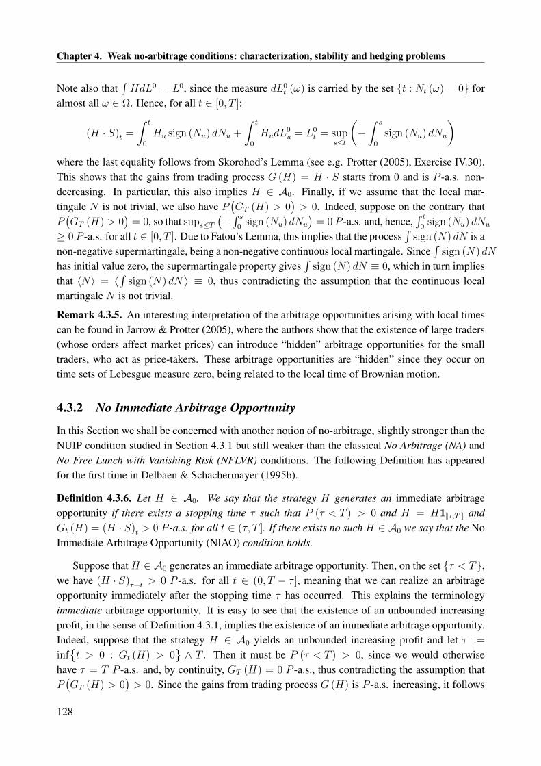
Chapter 4. Weak no-arbitrage conditions: characterization, stability and hedging problems
Note also that∫HdL0 = L0, since the measure dL0
t (ω) is carried by the set t : Nt (ω) = 0 foralmost all ω ∈ Ω. Hence, for all t ∈ [0, T ]:
(H · S)t =
∫ t
0
Hu sign (Nu) dNu +
∫ t
0
HudL0u = L0
t = sups≤t
(−∫ s
0
sign (Nu) dNu
)where the last equality follows from Skorohod’s Lemma (see e.g. Protter (2005), Exercise IV.30).This shows that the gains from trading process G (H) = H · S starts from 0 and is P -a.s. non-decreasing. In particular, this also implies H ∈ A0. Finally, if we assume that the local mar-tingale N is not trivial, we also have P
(GT (H) > 0
)> 0. Indeed, suppose on the contrary that
P(GT (H) > 0
)= 0, so that sups≤T
(−∫ s
0sign (Nu) dNu
)= 0 P -a.s. and, hence,
∫ t0
sign (Nu) dNu
≥ 0 P -a.s. for all t ∈ [0, T ]. Due to Fatou’s Lemma, this implies that the process∫
sign (N) dN is anon-negative supermartingale, being a non-negative continuous local martingale. Since
∫sign (N) dN
has initial value zero, the supermartingale property gives∫
sign (N) dN ≡ 0, which in turn impliesthat 〈N〉 =
⟨∫sign (N) dN
⟩≡ 0, thus contradicting the assumption that the continuous local
martingale N is not trivial.
Remark 4.3.5. An interesting interpretation of the arbitrage opportunities arising with local timescan be found in Jarrow & Protter (2005), where the authors show that the existence of large traders(whose orders affect market prices) can introduce “hidden” arbitrage opportunities for the smalltraders, who act as price-takers. These arbitrage opportunities are “hidden” since they occur ontime sets of Lebesgue measure zero, being related to the local time of Brownian motion.
4.3.2 No Immediate Arbitrage Opportunity
In this Section we shall be concerned with another notion of no-arbitrage, slightly stronger than theNUIP condition studied in Section 4.3.1 but still weaker than the classical No Arbitrage (NA) andNo Free Lunch with Vanishing Risk (NFLVR) conditions. The following Definition has appearedfor the first time in Delbaen & Schachermayer (1995b).
Definition 4.3.6. Let H ∈ A0. We say that the strategy H generates an immediate arbitrageopportunity if there exists a stopping time τ such that P (τ < T ) > 0 and H = H1]]τ,T ]] andGt (H) = (H · S)t > 0 P -a.s. for all t ∈ (τ, T ]. If there exists no such H ∈ A0 we say that the NoImmediate Arbitrage Opportunity (NIAO) condition holds.
Suppose that H ∈ A0 generates an immediate arbitrage opportunity. Then, on the set τ < T,we have (H · S)τ+t > 0 P -a.s. for all t ∈ (0, T − τ ], meaning that we can realize an arbitrageopportunity immediately after the stopping time τ has occurred. This explains the terminologyimmediate arbitrage opportunity. It is easy to see that the existence of an unbounded increasingprofit, in the sense of Definition 4.3.1, implies the existence of an immediate arbitrage opportunity.Indeed, suppose that the strategy H ∈ A0 yields an unbounded increasing profit and let τ :=
inft > 0 : Gt (H) > 0
∧ T . Then it must be P (τ < T ) > 0, since we would otherwise
have τ = T P -a.s. and, by continuity, GT (H) = 0 P -a.s., thus contradicting the assumption thatP(GT (H) > 0
)> 0. Since the gains from trading process G (H) is P -a.s. increasing, it follows
128

4.3 Characterization of weak no-arbitrage conditions
that the strategy H := H1]]τ,T ]] ∈ A0 realizes an immediate arbitrage opportunity. An example of amodel which satisfies the NUIP condition but which allows for immediate arbitrage opportunitieswill be presented at the end of this Section, thus showing that the NIAO condition is strictly strongerthan the NUIP condition.
Let us also give the following Definition, which formalizes an economically sound notion ofarbitrage opportunity.
Definition 4.3.7. Let H ∈ A0. We say that the strategy H generates a strong arbitrage opportunityif P(GT (H) > 0
)> 0. If there exists no such H ∈ A0, i.e.
GT (H) : H ∈ A0
∩ L0
+ = 0, wesay that the No Strong Arbitrage (NSA) condition holds.
The NSA condition introduced in Definition 4.3.7 corresponds to the NA+ property consideredin Strasser (2005). Intuitively, a strong arbitrage opportunity consists in a trading strategy whichdoes not require any initial capital nor any amount of credit at intermediate times and leads (withnon-zero probability) to a strictly positive final wealth. Of course, this sort of strategy should bebanned from any reasonable financial market model. We have the following simple Lemma.
Lemma 4.3.8. The NIAO condition and the NSA condition are equivalent.
Proof. By following the arguments used in the first part of the proof of Lemma 3.1 in Delbaen &Schachermayer (1995b), it can be shown that a strong arbitrage opportunity implies the existenceof an immediate arbitrage opportunity. Hence, NIAO implies NSA. Conversely, it is easy to seedirectly from Definitions 4.3.6 and 4.3.7 that an immediate arbitrage opportunity is also a strongarbitrage opportunity. Hence, NSA implies NIAO.
Remark 4.3.9 (On the NSA condition). Our definition of strong arbitrage opportunity is similarto the notion of arbitrage opportunity adopted in Loewenstein & Willard (2000). In particular, inthe context of a complete diffusion-based financial market model, Theorem 1 of Loewenstein &Willard (2000) shows that the absence of arbitrage opportunities should be regarded as a minimalcondition, in the absence of which there is no solution to any utility maximization problem. TheNSA condition has been also adopted as a minimal condition in Christensen & Larsen (2007), inlieu of the stronger classical No Arbitrage (NA) condition
GT (H) : H ∈ A
∩ L0
+ = 0. Fur-thermore, the notion of strong arbitrage opportunity corresponds to the notion of arbitrage adoptedin the context of the Benchmark Approach, see e.g. Section 10.3 of Platen & Heath (2006) andSection 7 of Platen (2009). However, we want to point out that typical applications of the bench-mark approach require stronger assumptions than the mere absence of strong arbitrage opportunities(or, equivalently, immediate arbitrage opportunities), namely the existence of the growth-optimalportfolio. In Karatzas & Kardaras (2007), the authors show that the existence of a non-explodinggrowth-optimal portfolio is equivalent to the No Unbounded Profit with Bounded Risk (NUPBR)condition. As we are going to show in Section 4.3.3, the NUPBR condition is strictly stronger thanthe NSA condition. This means that, in the context of the benchmark approach, not only strongarbitrage opportunities but also slightly weaker forms of arbitrage are ruled out from the market.
129

Chapter 4. Weak no-arbitrage conditions: characterization, stability and hedging problems
As we have seen, the NIAO condition (or, equivalently, the NSA condition) is stronger thanthe NUIP condition. Theorem 4.3.2 shows that the NUIP condition is equivalent to the existenceof an Rd-valued predictable process λ = (λt)0≤t≤T such that a = cλ holds P ⊗ B-a.e., where theprocesses a, c andB are as in (4.1). Hence, it seems natural to conjecture that the NIAO condition isequivalent to the existence of a process λ as above satisfying some additional integrability property.This conjecture is correct, as we are going to show in the following Theorem. As a preliminary, letus define the mean-variance tradeoff process K =
(Kt
)0≤t≤T as follows, for t ∈ [0, T ]:
Kt :=
∫ t
0
λ′ud〈M,M〉uλu =d∑
i,j=1
∫ t
0
λiuciju λ
judBu (4.4)
where the Rd-valued process λ = (λt)0≤t≤T is as in Theorem 4.3.2. Let also Kts := Kt−Ks, for all
s, t ∈ [0, T ] with s ≤ t. As in Levental & Skorohod (1995) and Strasser (2005), let us also definethe following stopping time:
α := inft > 0 : Kt+h
t =∞,∀h ∈ (0, T − t]
(4.5)
with the usual convention inf ∅ = ∞. The result of the following Theorem has been alreadyobtained in Strasser (2005), albeit with a slightly different proof.
Theorem 4.3.10. The NIAO condition holds if and only if there exists an Rd-valued predictableprocess λ = (λt)0≤t≤T such that a = cλ holds P ⊗B-a.e. and the stopping time α satisfies α =∞P -a.s., meaning that the process K does not jump to infinity.
Proof. We have already seen that the NIAO condition implies the NUIP condition. Hence, theexistence of an Rd-valued predictable process λ = (λt)0≤t≤T such that a = cλ holds P ⊗ B-a.e.follows from Theorem 4.3.2. The fact that the NIAO condition implies α = ∞ P -a.s. is shownin Theorem 3.6 of Delbaen & Schachermayer (1995b) (compare also with Kabanov & Stricker(2005), Section 3, and Strasser (2005), Theorem 3.5).
Conversely, suppose that there exists an Rd-valued predictable process λ = (λt)0≤t≤T such thata = cλ holds P ⊗ B-a.e. and α = ∞ P -a.s. and let the strategy H ∈ A0 yield an immediatearbitrage opportunity with respect to a stopping time τ with P (τ < T ) > 0. By assumption, sinceα = ∞ P -a.s., we have P
(Kτ+hτ =∞,∀h ∈ (0, T − τ ]
)= 0. For every n ∈ N, define the
stopping time ρn := inft > τ : Kt
τ ≥ n∧ T . Since K is continuous and does not jump to
infinity, it is clear that ρn > τ P -a.s. on the set τ < T, for all n ∈ N. Let us define the processλτ,n := λ1]]τ,ρn]], for every n ∈ N. Then, on the set τ < T:∫ T
0
(λτ,nt )′ d〈M,M〉tλτ,nt =
∫ T
0
1]]τ,ρn]]λ′td〈M,M〉tλt = Kρn
τ ≤ n P -a.s.
This implies that λτ,n ∈ L2 (M), for all n ∈ N, and we can meaningfully define the stochastic ex-ponential Zτ,n := E (−λτ,n ·M). The process Zτ,n is a strictly positive continuous local martingale(due to Novikov’s condition it is also a uniformly integrable martingale, see e.g. Protter (2005),
130

4.3 Characterization of weak no-arbitrage conditions
Theorem III.45). It is also obvious that Zτ,n ≡ 1 on the stochastic interval [[0, τ ]] and Zτ,n ≡ Zτ,nρn
on the stochastic interval ]]ρn, T ]]. Let us now compute the stochastic differential of the productZτ,n (H · S)ρn , where (H · S)ρn denotes the stochastic integral process H · S stopped at ρn:
d(Zτ,nt (H · S)ρnt
)= Zτ,n
t d (H · S)ρnt + (H · S)ρnt dZτ,nt + d
[Zτ,n, (H · S)ρn
]t
= Zτ,nt d (H ·M)ρnt + Zτ,n
t d (H · A)ρnt + (H · S)ρnt dZτ,nt − Z
τ,nt H ′td〈M,M〉tλτ,nt
= Zτ,nt d (H ·M)ρnt + (H · S)ρnt dZτ,n
t + Zτ,nt H ′t
(dAρnt − d〈M,M〉tλτ,nt
)= Zτ,n
t d (H ·M)ρnt + (H · S)ρnt dZτ,nt
(4.6)where the first equality follows from the integration by parts formula (see e.g. Protter (2005),Corollary 2 to Theorem II.22), the third equality uses the fact that Zτ,n
t d (H · A)ρnt = Zτ,nt H ′tdA
ρnt ,
since we have Zτ,n ∈ L (H · A) (being adapted and continuous, hence predictable and locallybounded) and H ∈ L (S), and, finally, the last equality is due to the fact that dA = d〈M,M〉λand H = H1]]τ,T ]]. Due to Theorem IV.29 of Protter (2005), equation (4.6) shows that the prod-uct Zτ,n (H · S)ρn is a non-negative local martingale and, due to Fatou’s Lemma, also a super-martingale, for all n ∈ N. Since Zτ,n
0 (H · S)ρn0 = 0, the supermartingale property implies thatZτ,nt (H · S)ρnt = 0 for all t ∈ [0, T ] P -a.s. Recall that, on the set τ < T, we have ρn > τ P -a.s.
and so Zτ,n > 0 P -a.s., for all n ∈ N. This implies that (H · S)ρn ≡ 0 on the set τ < T, forall n ∈ N. Hence, we can conclude that H · S ≡ 0 on
⋃n∈N ]]τ, ρn]]. Since P (τ < T ) > 0, this
contradicts the fact that (H · S)t > 0 P -a.s. for all t ∈ (τ, T ], thus showing that there cannot existan immediate arbitrage opportunity.
In particular, it is important to note that Theorem 4.3.10 shows that we can check whethera financial market model allows for immediate arbitrage opportunities by looking directly at thecharacteristics of the process S representing the discounted price of the risky assets.
Let us now formalize in the following Definition the concept of (weak) martingale deflator,which plays the role of a weaker counterpart to the classical concept of martingale measure (see thelast part of Section 4.3.3 for more details on this point) and bears a close similarity to the notion ofmartingale density introduced in Schweizer (1992),(1995).
Definition 4.3.11. Let Z = (Zt)0≤t≤T be a non-negative local martingale with Z0 = 1. We say thatZ is a weak martingale deflator if the product ZSi is a local martingale, for all i = 1, . . . , d. If Zsatisfies in addition ZT > 0 P -a.s. we say that Z is a martingale deflator.
Remark 4.3.12. Let the process Z = (Zt)0≤t≤T be a weak martingale deflator. Since Z is a non-negative local martingale, Fatou’s Lemma implies that Z is also a supermartingale (and, hence, atrue martingale if and only if E [ZT ] = E [Z0] = 1). Furthermore, if Z is a martingale deflator, sothat ZT > 0 P -a.s., the minimum principle for non-negative supermartingales (see e.g. Revuz &Yor (1999), Proposition II.3.4) implies that P
(Zt > 0 and Zt− > 0 for all t ∈ [0, T ]
)= 1.
The following Lemma shows the fundamental property of weak martingale deflators. For thedefinition and the main properties of σ-martingales we refer the reader to Section 2 of Delbaen &
131

Chapter 4. Weak no-arbitrage conditions: characterization, stability and hedging problems
Schachermayer (1998b), Section III.6e of Jacod & Shiryaev (2003), Kallsen (2004) and SectionIV.9 of Protter (2005). Observe that the following Lemma does not rely on the continuity of Sbut holds true also in the more general context where S is a general (possibly discontinuous andnon-locally bounded) semimartingale.
Lemma 4.3.13. Let the process Z = (Zt)0≤t≤T be a weak martingale deflator. Then, for anyH ∈ L (S), the product Z (H · S) is a σ-martingale. If in addition H ∈ A, then the productZ (H · S) is a local martingale.
Proof. Let Z = (Zt)0≤t≤T be a weak martingale deflator and let H ∈ L (S). Define the Rd+1-valued local martingale Y = (Yt)0≤t≤T by Yt :=
(ZtS
1t , . . . , ZtS
dt , Zt
)′ and let L (Y ) be the set ofall Rd+1-valued predictable Y -integrable processes, in the sense of Definition III.6.17 of Jacod &Shiryaev (2003). For all n ∈ N, define also Hn := H1‖H‖≤n. Then, using twice the integrationby parts formula:
Z(H (n) · S
)= Z− ·
(H (n) · S
)+(H (n) · S
)− · Z +
[Z,H (n) · S
]=(Z−H (n)
)· S +
(H (n) · S
)− · Z +H (n) · [S,Z]
= H (n) · (ZS − S− · Z) +(H (n) · S
)− · Z
= H (n) · (ZS) +((H (n) · S
)− −H (n)′ S−
)· Z = K (n) · Y
where, for every n ∈ N, the Rd+1-valued predictable process K (n) is defined as K (n)i := H (n)i,for all i = 1, . . . , d, and K (n)d+1 :=
(H (n) · S
)− −H (n)′ S−. Clearly, we have K (n) ∈ L (Y ),
sinceK (n) is a predictable and locally bounded process, for all n ∈ N. Define also the Rd+1-valuedpredictable process K by Ki := H i, for all i = 1, . . . , d, and Kd+1 := (H · S)− −H ′S−. Arguingas in the proof of Proposition 8 of Rheinländer & Schweizer (1997), note that H (n) · S convergestoH ·S in the semimartingale topology as n→∞, sinceH ∈ L (S). This implies thatK (n) ·Y =
Z(H (n) ·S
)also converges in the semimartingale topology, since the multiplication with the fixed
semimartingale Z is a continuous operation. Since the spaceK · Y : K ∈ L (Y )
is closed in the
semimartingale topology (see e.g. Jacod & Shiryaev (2003), Proposition III.6.26), we can concludethat Z (H · S) = K ·Y for some K ∈ L (Y ). But since K (n) converges to K (P -a.s. uniformly int, at least along a subsequence) as n→∞, we can conclude that K = K; see Mémin (1980). Thisshows thatK ∈ L (Y ). Since the process Y is a local martingale andK ∈ L (Y ), Theorem IV.90 ofProtter (2005) implies that Z (H · S) = K ·Y is a σ-martingale. Now, to prove the second assertionof the Lemma, suppose that we also have H ∈ A. Then, due to Definition 4.2.2, there exists apositive constant a such that (H · S)t ≥ −a P -a.s. for all t ∈ [0, T ]. The process Z (a+H · S) is aσ-martingale, being the sum of a local martingale and a σ-martingale. Furthermore, Exercise IV.43of Protter (2005) (see also Kallsen (2004), Proposition 3.1) implies that Z (a+H · S) is a localmartingale and also a supermartingale, being a non-negative σ-martingale. In turn, this implies thatthe process Z (H · S) is a local martingale, being the difference of two local martingales.
If the process Z = (Zt)0≤t≤T is a weak martingale deflator and H ∈ A1, Lemma 4.3.13 impliesthat Z (1 +H · S) is a non-negative local martingale and, hence, a supermartingale. According to
132

4.3 Characterization of weak no-arbitrage conditions
the terminology adopted in Becherer (2001), this means that the process Z = (Zt)0≤t≤T is a P -supermartingale density. Similarly, if Z is a martingale deflator, Lemma 4.3.13 implies that Z is anequivalent supermartingale deflator in the sense of Definition 4.9 of Karatzas & Kardaras (2007).The importance of supermartingale densities/deflators has been first recognized by Kramkov &Schachermayer (1999).
Our next goal consists in showing that the NIAO condition ensures the existence of a weakmartingale deflator. This can already be guessed by following the arguments used in the sec-ond part of the proof of Theorem 4.3.10, but we prefer to give full details. So, let us supposethat the NIAO condition holds and define the stopping time τ := inf
t ∈ [0, T ] : Kt = ∞
.
Then, due to Theorem 4.3.10, we have α = ∞ P -a.s. and, hence, τ > 0 P -a.s. (see also Del-baen & Schachermayer (1995b), Theorem 3.6). Let the process λ = (λt)0≤t≤T be as in Theorem4.3.10. Then, on the stochastic interval [[0, τ [[ , the stochastic integral λ · M is well-defined asa continuous local martingale. This allows us to define the process Z := E (−λ ·M)1[0,τ) =
exp(−λ ·M − 1
2
∫λ′d〈M,M〉λ
)1[0,τ). On the set τ ≤ T, the process Z hits zero not by a jump
and we haveZτ− = 0
=Kτ = ∞
, see also Section 4 of Kabanov & Stricker (2005). The
process Z is well-defined as a continuous local martingale (and furthermore, being non-negative,Fatou’s Lemma implies that it is a supermartingale). On the stochastic interval [[0, τ [[ , the samecalculations as in (4.6) allow to show the following, for any H ∈ L (S):
Z (H · S) =(ZH
)·M + (H · S) · Z
where we have also used the continuity of Z and S. Since H ∈ L (S) ⊆ L2loc (M) and Z is adapted
and continuous, hence predictable and locally bounded, we have ZH ∈ L2loc (M). Similarly, we
also have H · S ∈ L2loc
(Z). This shows that the process Z (H · S) is a continuous local martingale
on the stochastic interval [[0, τ [[ . Since Z remains frozen at zero after τ and Zτ = Zτ− on τ ≤ T,this implies that the process Z (H · S) is a continuous local martingale on the whole interval [0, T ].In a similar way, using the fact that, as a consequence of Theorem 4.3.10, we have dA = d〈M,M〉λ,we can easily show that ZSi is also a continuous local martingale, for all i = 1, . . . , d. Furthermore,the process Z is such that, for any local martingale N = (Nt)0≤t≤T strongly orthogonal (in thesense of Jacod & Shiryaev (2003), Definition I.4.11) to the local martingale partM in the canonicaldecomposition of S, the product ZN is a local martingale. This can be easily shown as follows:
ZN = Z− ·N +N− · Z +[Z, N
]= Z ·N +N− · Z − Zλ · 〈M,N〉 = Z ·N +N− · Z
where we have used the continuity of M and the orthogonality of M and N . Since the processes Zand N− are predictable and locally bounded, being adapted and left-continuous, and since Z and Nare both local martingales, Theorem IV.29 of Protter (2005) implies that ZN is a local martingale.Summing up, we have proved the following Proposition.
Proposition 4.3.14. Suppose that the NIAO condition holds and let τ :=inft ∈ [0, T ] : Kt=∞
.
Then the process Z := E (−λ ·M)1[0,τ) is a weak martingale deflator. Furthermore, for any localmartingale N = (Nt)0≤t≤T strongly orthogonal to the local martingale part M in the canonicaldecomposition of S, the product ZN is a local martingale.
133

Chapter 4. Weak no-arbitrage conditions: characterization, stability and hedging problems
Remark 4.3.15 (On the minimal martingale measure). The process Z := E (−λ ·M) representsthe candidate density process of the so-called minimal martingale measure, originally introduced byFöllmer & Schweizer (1991) and formally defined as a probability measure Q on (Ω,F) such thatQ = P onF0 and Q ∼ P , such that S is a local Q-martingale and such that Q preserves orthogonal-ity, in the sense that every local P -martingale which is strongly P -orthogonal to the martingale partM in the canonical decomposition of S (with respect to P ) is also a local Q-martingale. Proposition4.3.14 shows that the process Z is a weak martingale deflator and possesses such an orthogonality-preserving property. However, the process Z can fail to be the well-defined density process of theminimal martingale measure Q for two reasons. First, it could be that P
(ZT > 0
)< 1, so that
the measure Q on (Ω,F) defined by dQdP
:= ZT would fail to be equivalent to P , being only ab-solutely continuous to P . Second, Z may fail to be a true martingale, being instead a strict localmartingale (and a strict supermartingale), i.e. a local martingale which is not a true martingale,meaning that E
[ZT]< E
[Z0
]= 1. In the latter case, Q would fail to be a probability measure,
since Q (Ω) = E[ZT]< 1.
Remark 4.3.16 (On the tradeability of Z). The weak martingale deflator Z introduced in Propo-sition 4.3.14 has another interesting property. To see that, let us define the process X := 1/Z − 1
on the stochastic interval [[0, τ [[ . On the setZτ = 0
we let Xτ− = Xτ = ∞ and, since after τ
the process Z remains frozen at 0, we extend X in a natural way on the stochastic interval [[τ, T ]]
by letting X =∞. Note that, as soon as the NIAO condition holds, the stochastic integrals H ·Mand H · S are well-defined on the stochastic interval [[0, τ [[ and, hence, the process X satisfies thefollowing:
dXt = −Z−2t dZt + Z−3
t d⟨Z⟩t
= Z−1t λtdMt + Z−1
t λ′td〈M,M〉tλt = HtdSt
where the Rd-valued predictable process H ∈ L (S) is defined as H := Z−1λ. Since X ≥ −1 P -a.s., we also have that the strategy H is 1-admissible, i.e. H = Z−1λ ∈ A1. This means that, usingthe terminology introduced in Section 4.4 of Karatzas & Kardaras (2007), the weak martingaledeflator Z is tradeable, since it can be represented as the wealth process associated to a suitable 1-admissible trading strategy. Related results can also be found in Delbaen & Schachermayer (1995b)and Kabanov & Stricker (2005).
We conclude this Section by showing an example of a model which satisfies the NUIP conditionbut which allows for immediate arbitrage opportunities. In view of Theorem 4.3.10, the examplebelow exhibits a model which satisfies the weak structure condition dA d〈M,M〉 but for whichP (α < T ) > 0.
Example 4.3.17. This Example is a generalization of Example 3.4 of Delbaen & Schachermayer(1995b). Let M = (Mt)0≤t≤T be a real-valued continuous local martingale with M0 = 0 on thefiltered probability space (Ω,F ,F, P ) and define the discounted price process S = (St)0≤t≤T of asingle risky asset as S := M + 〈M〉γ , for some γ ≤ 1/2. Then, due to Itô’s formula:
dSt = dMt + γ〈M〉γ−1t d〈M〉t
134
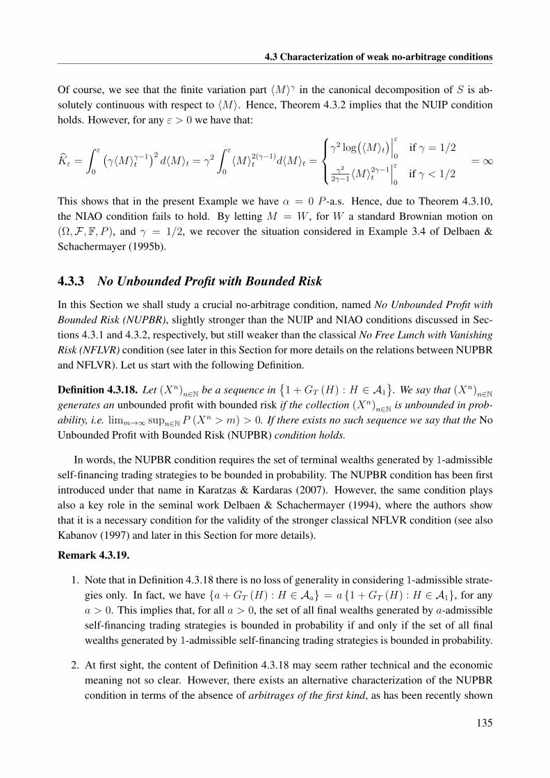
4.3 Characterization of weak no-arbitrage conditions
Of course, we see that the finite variation part 〈M〉γ in the canonical decomposition of S is ab-solutely continuous with respect to 〈M〉. Hence, Theorem 4.3.2 implies that the NUIP conditionholds. However, for any ε > 0 we have that:
Kε =
∫ ε
0
(γ〈M〉γ−1
t
)2d〈M〉t = γ2
∫ ε
0
〈M〉2(γ−1)t d〈M〉t =
γ2 log
(〈M〉t
)∣∣∣ε0
if γ = 1/2
γ2
2γ−1〈M〉2γ−1
t
∣∣∣ε0
if γ < 1/2=∞
This shows that in the present Example we have α = 0 P -a.s. Hence, due to Theorem 4.3.10,the NIAO condition fails to hold. By letting M = W , for W a standard Brownian motion on(Ω,F ,F, P ), and γ = 1/2, we recover the situation considered in Example 3.4 of Delbaen &Schachermayer (1995b).
4.3.3 No Unbounded Profit with Bounded Risk
In this Section we shall study a crucial no-arbitrage condition, named No Unbounded Profit withBounded Risk (NUPBR), slightly stronger than the NUIP and NIAO conditions discussed in Sec-tions 4.3.1 and 4.3.2, respectively, but still weaker than the classical No Free Lunch with VanishingRisk (NFLVR) condition (see later in this Section for more details on the relations between NUPBRand NFLVR). Let us start with the following Definition.
Definition 4.3.18. Let (Xn)n∈N be a sequence in
1 + GT (H) : H ∈ A1
. We say that (Xn)n∈N
generates an unbounded profit with bounded risk if the collection (Xn)n∈N is unbounded in prob-ability, i.e. limm→∞ supn∈N P (Xn > m) > 0. If there exists no such sequence we say that the NoUnbounded Profit with Bounded Risk (NUPBR) condition holds.
In words, the NUPBR condition requires the set of terminal wealths generated by 1-admissibleself-financing trading strategies to be bounded in probability. The NUPBR condition has been firstintroduced under that name in Karatzas & Kardaras (2007). However, the same condition playsalso a key role in the seminal work Delbaen & Schachermayer (1994), where the authors showthat it is a necessary condition for the validity of the stronger classical NFLVR condition (see alsoKabanov (1997) and later in this Section for more details).
Remark 4.3.19.
1. Note that in Definition 4.3.18 there is no loss of generality in considering 1-admissible strate-gies only. In fact, we have a+GT (H) : H ∈ Aa = a 1 +GT (H) : H ∈ A1, for anya > 0. This implies that, for all a > 0, the set of all final wealths generated by a-admissibleself-financing trading strategies is bounded in probability if and only if the set of all finalwealths generated by 1-admissible self-financing trading strategies is bounded in probability.
2. At first sight, the content of Definition 4.3.18 may seem rather technical and the economicmeaning not so clear. However, there exists an alternative characterization of the NUPBRcondition in terms of the absence of arbitrages of the first kind, as has been recently shown
135

Chapter 4. Weak no-arbitrage conditions: characterization, stability and hedging problems
in Kardaras (2010a). Formally, an arbitrage of the first kind is defined as a non-negativeF-measurable random variable ξ with P (ξ > 0) > 0 such that for all x > 0 there exists anx-admissible strategy Hx ∈ Ax satisfying x+GT (Hx) ≥ ξ P -a.s.
As we have seen in Sections 4.3.1 and 4.3.2, the NUIP and NIAO conditions exclude ratherblatant forms of arbitrage, which can be seen as pathologies of a given financial market model.The NUIP and NIAO conditions can therefore be regarded as indispensable “sanity checks” for anyfinancial market model. However, they do not guarantee the solvability of fundamental problemsin financial mathematics such as portfolio optimization, valuation and hedging problems. Theresult of Proposition 4.19 of Karatzas & Kardaras (2007) is therefore of great interest, since itshows that the failure of the NUPBR condition precludes the solvability of any utility maximizationproblem. In the particular case of a complete diffusion-based financial market model, an analogousresult has already been shown in Loewenstein & Willard (2000). Furthermore, as soon as theNUPBR condition holds, the benchmark approach proposed by Eckhard Platen and co-authorsprovides a coherent framework for dealing with valuation and hedging problems for non-negativecontingent claims, see e.g. Platen (2006), Platen & Heath (2006) and Platen (2009). Under theNUPBR condition, but not requiring the full strength of the classical NFLVR condition, valuationand hedging problems are also dealt with in Fernholz & Karatzas (2009), Fontana & Runggaldier(2011) and Ruf (2011b) in the context of diffusion-based financial market models. Summing up,these observations imply that the NUPBR condition not only excludes strong forms of arbitragefrom the market but also opens the doors to the solution of classical problems of mathematicalfinance and, hence, can be regarded as the fundamental no-arbitrage condition.
It is easy to show that if there is an immediate arbitrage opportunity, in the sense of Definition4.3.6, then there is also an unbounded profit with bounded risk, meaning that the NUPBR conditionis stronger than the NIAO condition. In fact, suppose that the strategy H ∈ A0 generates animmediate arbitrage opportunity with respect to a stopping time τ with P (τ < T ) > 0. Let ξ :=
GT (H) = 1τ<T (H · S)T , so that P (ξ ≥ 0) = 1 and P (ξ > 0) > 0. For all n ∈ N, let us definethe processHn := nH ∈ A0 ⊆ A1 and theF-measurable random variableXn := 1+(Hn · S)T =
1 + nξ. Clearly, the collection (Xn)n∈N ⊆
1 +GT (H) : H ∈ A1
is not bounded in probability,
meaning that (Xn)n∈N generates an unbounded profit with bounded risk. Equivalently (see part 2of Remark 4.3.19), the F-measurable random variable ξ is an arbitrage of the first kind. In fact, forall x > 0, we have x + GT (H) = x + ξ > ξ. An example of a model which satisfies the NIAOcondition but which allows for an unbounded profit with bounded risk will be presented later in thisSection, thus showing that the NUPBR condition is strictly stronger than the NIAO condition.
We now continue the study of the NUPBR condition by giving an equivalent criterion for itsvalidity. To this effect, let us first introduce the following Definition3, which is adapted fromChristensen & Larsen (2007).
Definition 4.3.20. Let (Hn)n∈N be a sequence in L (S) with Hn · S ≥ −1/n for all n ∈ N. Wesay that (Hn)n∈N generates an approximate arbitrage opportunity if GT (Hn) → f in probability
3We warn the reader that in Levental & Skorohod (1995) the term approximate arbitrage is used with a differentmeaning.
136

4.3 Characterization of weak no-arbitrage conditions
as n→∞, for some F-measurable non-negative random variable f such that P (f > 0) > 0.
Lemma 4.3.21. The NUPBR condition holds if and only if there do not exist approximate arbitrageopportunities.
Proof. It is clear that the set
1 + (H · S)T : H ∈ A1
cannot be bounded in probability if
there exists a sequence (Hn)n∈N which generates an approximate arbitrage opportunity. In fact,the strategy nHn is 1-admissible, for every n ∈ N, and the collection
1 + n (Hn · S)T : n ∈ N
is unbounded in probability (compare also with Delbaen & Schachermayer (1994), Proposition3.6). Conversely, suppose that the NUPBR condition fails to hold. Then there exists a sequence(Hn)n∈N ⊆ A1 such that P
((Hn · S)T ≥ n
)> β for all n ∈ N and for some β > 0. For every
n ∈ N, let Hn := 1nHn. Clearly, we have Hn ∈ A1/n and P
((Hn · S)T ≥ 1
)> β, for all
n ∈ N. Let gn := 1n
+(Hn · S
)T≥ 0 P -a.s., for all n ∈ N. Due to Lemma A1.1 of Delbaen &
Schachermayer (1994), there exists a sequence (fn)n∈N, with fn ∈ conv gn, gn+1, . . ., such that(fn)n∈N converges P -a.s. to a non-negative F-measurable random variable f . For all n ∈ N, letKn be the convex combination of the strategies
(Hm)m≥n corresponding to fn. It is easy to see
that Kn ∈ A1/n, for all n ∈ N. Furthermore, we have GT (Kn) = (Kn · S)T = fn + O (n−1),so that GT (Kn) → f P -a.s. and, hence, also in probability, as n → ∞. Furthermore, due to thelast part of Lemma A1.1 of Delbaen & Schachermayer (1994), we have that P (f > 0) > 0, thusshowing that the sequence (Kn)n∈N generates an approximate arbitrage opportunity.
Remark 4.3.22 (On approximate arbitrage opportunities and cheap thrills). The notion ofapproximate arbitrage opportunity is closely related to the concept of cheap thrill introduced inLoewenstein & Willard (2000). Formally, a cheap thrill is defined as a sequence (Hn)n∈N ⊆ L (S)
such thatHn ∈ Axn , for some xn ≥ 0, for all n ∈ N, with xn 0 as n→∞ and xn+GT (Hn)→∞ P -a.s. as n → ∞ on some set with non-zero probability. By reasoning as in the first part ofthe proof of Lemma 4.3.21, it can be easily shown that the set
1 + GT (H) : H ∈ A1
cannot
be bounded in probability if there exists a cheap thrill and, hence, due to Lemma 4.3.21, thereexists an immediate arbitrage opportunity. Conversely, one can easily construct a cheap thrill froma sequence (Hn)n∈N ⊆ L (S) which generates an approximate arbitrage opportunity. In fact, forall n ∈ N, let xn := log(n)
nand Hn := log (n)Hn. Then xn + Hn · S = log (n)
(1n
+Hn · S)≥ 0
P -a.s., since Hn ∈ A1/n, so that we have Hn ∈ Axn , for all n ∈ N. Furthermore, we have xn 0
as n → ∞. By assumption, GT (Hn) = (Hn · S)T → f in probability as n → ∞, for some F-measurable non-negative random variable f with P (f > 0) > 0. Passing to a subsequence, we canassume that the convergence takes place P -a.s. This implies GT
(Hn
)= log (n)GT (Hn) → ∞
P -a.s. as n → ∞ on some set with strictly positive probability, thus showing that there exists acheap thrill.
Summing up, by combining part 2 of Remark 4.3.19, Lemma 4.3.21 and Remark 4.3.22, wehave shown the equivalence between the following types of arbitrage opportunities:
• unbounded profit with bounded risk;
• arbitrage of the first kind;
137

Chapter 4. Weak no-arbitrage conditions: characterization, stability and hedging problems
• approximate arbitrage;
• cheap thrill.
We want to emphasize that all the above forms of arbitrage opportunities are stronger than theclassical Free Lunch with Vanishing Risk notion adopted in the context of the classical no-arbitragetheory as formulated in Delbaen & Schachermayer (1994),(1998b),(2006).
The following Theorem gives necessary and sufficient conditions for the validity of NUPBR inthe context of general financial market models based on continuous semimartingales.
Theorem 4.3.23. The following are equivalent:
(a) the NUPBR condition holds;
(b) there exists an Rd-valued predictable process λ = (λt)0≤t≤T such that a = cλ holds P ⊗B-a.e. and KT <∞ P -a.s., i.e. λ ∈ L2
loc (M);
(c) there exists a martingale deflator (in the sense of Definition 4.3.11).
Proof. We first show that (a) implies (b). We already know that the NUPBR condition is strongerthan the NIAO condition. Hence, due to Theorem 4.3.10, there exists an Rd-valued predictableprocess λ = (λt)0≤t≤T such that a = cλ holds P ⊗ B-a.e. and α := inf
t > 0 : Kt+h
t =∞,∀h ∈(0, T − t]
= ∞ P -a.s. It remains to show that KT < ∞ P -a.s. Suppose that, on the contrary,
we have P (τ ≤ T ) > 0, where τ := inft ∈ [0, T ] : Kt = ∞
, so that P
(ZT = 0
)= P
(KT =
∞)> 0, where the process Z is defined as in Proposition 4.3.14. Define the sequence of stopping
times (τn)n∈N by τn := inft ∈ [0, T ] : Kt ≥ n
, for every n ∈ N. Clearly, we have τn τ P -a.s.
as n→∞. For all n ∈ N, define the Rd-valued predictable process λn := λ1]]0,τn]] and note that:∫ T
0
(λnt )′ d〈M,M〉tλnt =
∫ T
0
λt1]]0,τn]]d〈M,M〉tλt = KT∧τn ≤ n P -a.s.
This implies that λn ∈ L2 (M) and, since dA = d〈M,M〉λ (due to Theorem 4.3.2), we also haveλn ∈ L0 (A), for all n ∈ N. Hence, we can conclude that λn ∈ L (S), for all n ∈ N. Furthermore,KT∧τn < ∞ P -a.s. implies that the stopped process Zτn satisfies Zτn > 0 P -a.s. and, hence, theprocess
(Zτn)−1 is well-defined for all n ∈ N. Being adapted and continuous, the process
(Zτn)−1
is also predictable and locally bounded, for all n ∈ N. Thus, we have that(Zτn)−1
λn ∈ L (S) forall n ∈ N. As in Remark 4.3.16, a simple application of Itô’s formula gives the following, for everyn ∈ N: (
Zτn)−1 − 1 =
((Zτn)−1
λn)· S (4.7)
Since Zτn > 0 P -a.s., this also gives(Zτn)−1
λn ∈ A1, meaning that the strategyHn := Z−1λ1]]0,τn]]
=(Zτn)−1
λn ∈ L (S) is 1-admissible for all n ∈ N. Furthermore:
1 + (Hn · S)T =1
ZT∧τn→ 1
ZT∧τP -a.s. as n→∞
138

4.3 Characterization of weak no-arbitrage conditions
Since ZT∧τ = 0 on the setKT =∞
, which is supposed to have strictly positive probability, this
shows that the collection
1 +GT (Hn) : n ∈ N
is not bounded in probability, thus contradictingthe assumption that NUPBR holds.
Let us now show that (b) implies (c). If λ ∈ L2loc (M) the stochastic integral λ ·M is well-
defined as a continuous local martingale. Moreover, the stochastic exponential Z := E (−λ ·M)
is well-defined on the whole interval [0, T ] as a P -a.s. strictly positive continuous local martingalewith Z0 = 1. Similarly to (4.6), the product rule, together with the fact that dA = d〈M,M〉λ,allows to show that, for all i = 1, . . . , d:
d(ZtS
it
)= ZtdS
it+S
itdZt+d
[Si, Z
]t
= ZtdMit+S
itdZt+Zt
(dAit−d〈M i,M〉tλt
)= ZtdM
it+S
itdZt
where we have also used the continuity of Z and Si. This shows that ZSi is a local martingale forall i = 1, . . . , d, meaning that Z is a martingale deflator.
Finally, it remains to show that (c) implies (a). Let the process Z = (Zt)0≤t≤T be a martingaledeflator and let H ∈ A1. Then, due to Lemma 4.3.13, the product Z
(1+(H · S)
)is a non-negative
continuous local-martingale and, hence, also a supermartingale, so that E[ZT(1 + (H · S)T
)]≤
E[Z0
(1 + (H · S)0
)]= 1, for allH ∈ A1. This shows that the set
ZT(1 + (H · S)T
): H ∈ A1
is bounded in L1 (P ) and, therefore, it is also bounded in probability. Since the multiplication bythe finite random variable ZT does not affect the boundedness in probability, this implies that the set
1 +GT (H) : H ∈ A1
is bounded in probability, meaning that the NUPBR condition holds.
We want to point out that results analogous to Theorem 4.3.23 have already been obtained inSection 4 of Kardaras (2010a) and Section 3 of Hulley & Schweizer (2010), always in the contextof general financial market models driven by continuous sermimartingales. However, our proof ofTheorem 4.3.23 emphasizes the role of the process Z = E (−λ ·M) as the natural martingale de-flator. Furthermore, our proof of Theorem 4.3.23 highlights the fact that the process Z is tradeable,in the sense of Remark 4.3.16, and, hence, the event
ZT = 0
corresponds to the explosion of
the final wealth generated by a suitable 1-admissible self-financing trading strategy. For a relateddiscussion, see also Section 6 of Christensen & Larsen (2007).
Note that, due to the equivalence between conditions (a) and (b) in Theorem 4.3.23, as soonas the NUPBR condition holds we have
∫ T0λ′td〈M,M〉λt = KT < ∞ P -a.s. and so ZT =
E (−λ ·M)T > 0 P -a.s. Due to the supermartingale property, this also implies P(Zt > 0 for all t ∈
[0, T ])
= 1. If compared with the previous results concerning the NIAO condition (see Remark4.3.15), this implies that the process Z =
(Zt)
0≤t≤T can fail to be the well-defined density processof a probability measure Q on (Ω,F) with Q ∼ P and such that S is a local Q-martingale for onlyone reason: Z can fail to be a true martingale, being instead a strict local martingale. In the lattercase we would have E
[ZT]< E
[Z0
]= 1 and so letting dQ
dP:= ZT would not define a probability
measure on (Ω,F). In the recent paper Kardaras (2010a) it is shown that the existence of a mar-tingale deflator is equivalent to the existence of a finitely additive measure Q on (Ω,F), weaklyequivalent to P and only locally countably additive (hence, Q is not a true probability measure),under which the discounted price process S of the risky assets has a sort of local martingale be-havior (see also Section 5 of Cassese (2005) for some related results). The following Proposition
139

Chapter 4. Weak no-arbitrage conditions: characterization, stability and hedging problems
shows the general structure of all martingale deflators. Note that a martingale deflator does notnecessarily have to be continuous.
Proposition 4.3.24. Suppose that the NUPBR condition holds. Then a process Z = (Zt)0≤t≤T is amartingale deflator, in the sense of Definition 4.3.11, if and only if it can be written as follows:
Z = E (−λ ·M +N) = Z E (N) (4.8)
for some local martingale N = (Nt)0≤t≤T strongly orthogonal to M with N0 = 0 and ∆N > −1
P -a.s.
Proof. Let Z = (Zt)0≤t≤T be a martingale deflator. Due to Remark 4.3.12, we know that Z isa local martingale with P
(Zt > 0 and Zt− > 0 for all t ∈ [0, T ]
)= 1. Since the process Z− is
adapted and left-continuous, it is also predictable and locally bounded. These observations, togetherwith Theorem IV.29 of Protter (2005), imply that the stochastic integral process L := Z−1
− · Z iswell-defined as a local martingale with L0 = 0. Clearly, the local martingale L is the stochasticlogarithm of Z, meaning that we can write Z = E (L), see e.g. Theorem II.8.3 of Jacod & Shiryaev(2003). Since the martingale part M in the canonical decomposition of S is continuous, L admitsa Galtchouk-Kunita-Watanabe decomposition with respect to M , see Ansel & Stricker (1993). So,we can write:
L = ψ ·M +N
for some Rd-valued predictable process ψ = (ψt)0≤t≤T such that ψ ∈ L2loc (M) and a local martin-
gale N = (Nt)0≤t≤T strongly orthogonal to M with N0 = 0. Then, for all i = 1, . . . , d:
ZSi = Z− · Si + Si− · Z +[Z, Si
]= Z− · Ai + Z− ·M i + Si− · Z +
[Z,M i
]+[Z,Ai
]= Z− ·
(∫d〈M i,M〉λ
)+ Z− ·M i + Si− · Z + Z− ·
[ψ ·M +N,M i
]+[Z,Ai
]= Z− ·
(∫d〈M i,M〉 (λ+ ψ)
)+ Z− ·M i + Si− · Z + Z− ·
[N,M i
]+[Z,Ai
] (4.9)
Observe now that Z− ·M i and Si− · Z are both local martingales (see e.g. Protter (2005), TheoremIV.29). Furthermore, Z− · [N,M i] is a local martingale, since [N,M i] is a local martingale due tothe strong orthogonality of N and M , and [Z,Ai] is also a martingale due to Yoeurp’s Lemma (seee.g. Jacod & Shiryaev (2003), Proposition I.4.49). Hence, equation (4.9) implies that the processZ− ·
(∫d〈M i,M〉 (λ+ ψ)
)is a local martingale, for all i = 1, . . . , d. Being a predictable process
of finite variation, Theorem III.15 of Protter (2005) implies that it is also constant and P -a.s. equalto 0. Since Z− > 0 P -a.s., this means that
∫d〈M i,M〉 (λ+ ψ) ≡ 0 for all i = 1, . . . , d, which
in turn gives∫ T
0(λt + ψt)
′ d〈M,M〉t (λt + ψt) = 0 P -a.s. This implies that the stochastic integralψ ·M is indistinguishable from −λ ·M , thus yielding the following representation:
Z = E (ψ ·M +N) = E (−λ ·M +N) = Z E (N)
where the last equality follows by using the definition of Z and Yor’s formula (see Protter (2005),Theorem II.38), since [M,N ] = 〈M,N〉 = 0 due to the continuity of M and the strong orthogo-nality of M and N . Since Z > 0 and Z > 0 P -a.s., we also have E (N) > 0 P -a.s., meaning that
140

4.3 Characterization of weak no-arbitrage conditions
∆N > −1 P -a.s. Conversely, if Z = (Zt)0≤t≤T is a process which admits the representation (4.8),then Z is obviously a P -a.s. strictly positive local martingale with Z0 = 1, due to the definitionof stochastic exponential. Furthermore, analogous computations as in (4.9) allow to show that ZSi
is a local martingale for all i = 1, . . . , d. Due to Definition 4.3.11, we can conclude that Z is amartingale deflator.
Theorem 4.3.23 and Proposition 4.3.24 show that the process Z = E (−λ ·M) can be rightfullyconsidered as the minimal and natural martingale deflator. Indeed, if Z fails to be a well-definedmartingale deflator then there cannot exist any martingale deflator.
Remark 4.3.25 (Extension to discontinuous semimartingales). We want to point out that thecontinuity of S does not play a crucial role in the proof of Proposition 4.3.24. In fact, suppose thatthe semimartingale S is not necessarily continuous but only locally square-integrable, in the senseof Definition II.2.27 of Jacod & Shiryaev (2003). Then, any martingale deflator Z = (Zt)0≤t≤Tsuch that Z is locally square-integrable can be represented as Z = E (−λ ·M +N) for somelocally square-integrable local martingale N = (Nt)0≤t≤T strongly orthogonal to M with N0 = 0.In fact, the process L := Z−1
− ·Z is well-defined as a locally square-integrable local martingale (seeProtter (2005), Theorem IV.28) with L0 = 0 and, as such, it admits a Galtchouk-Kunita-Watanabedecomposition with respect to M , since M is also a locally square-integrable local martingale,see Ansel & Stricker (1993). Then, the computations in (4.9) and the remaining part of the proofof Proposition 4.3.24 do not rely on the continuity of M . However, note that under the presentassumptions we cannot write Z = Z E (N), since the process [M,N ] is not necessarily equalto zero. Analogous results have been already obtained in Theorem 1 of Schweizer (1995) andTheorem 2.2 and Corollary 2.3 of Choulli & Stricker (1996) (compare also with Christensen &Larsen (2007), Lemma 6.3). We also want to point out that the equivalence between (a) and (b) inTheorem 4.3.23 holds true also in the more general context where the discounted price process Sof the risky assets is a general (possibly discontinuous and non-locally bounded) semimartingale,as has been recently shown in Kardaras (2010b) and Takaoka (2010).
Let us now exhibit a simple example of a model which satisfies the NIAO condition but forwhich the NUPBR condition fails to hold. A similar example can also be found in Section 3.1 ofLoewenstein & Willard (2000).
Example 4.3.26. Let W = (Wt)0≤t≤T be a standard Brownian motion on (Ω,F ,F, P ) and definethe discounted price process S = (St)0≤t≤T of a single risky asset as the solution to the followingSDE, for some fixed K > 0:
dSt = St
(K − log (St)
T − t+
1
2
)dt+ St dWt S0 = 1 (4.10)
The SDE (4.10) admits an unique strong solution S, which also satisfies St > 0 P -a.s. for allt ∈ [0, T ]. If we let Xt := log (St), Itô’s formula gives the following:
dXt =K −Xt
T − tdt+ dWt X0 = 0
141

Chapter 4. Weak no-arbitrage conditions: characterization, stability and hedging problems
This shows that X is a Brownian bridge (see e.g. Revuz & Yor (1999), Exercise IX.2.12) startingat time t = 0 at the level 0 and ending at time t = T at the level K > 0. From (4.10) it is easy tosee that the conditions of Theorem 4.3.10 are satisfied and, hence, there are no immediate arbitrage
opportunities, thus implying that the process K =∫ ·
0
(K−log(Su)
T−u + 12
)2
du does not jump to infinity.
However, we have Kt < ∞ P -a.s. for all t ∈ [0, T ) but KT = ∞ P -a.s. Theorem 4.3.23 thenimplies that the NUPBR condition fails to hold.
We close this Section by discussing the relations between the NUPBR condition and the clas-sical No Arbitrage (NA) and No Free Lunch with Vanishing Risk (NFLVR) conditions, formallydefined as follows.
Definition 4.3.27. Let C :=(GT (H) : H ∈ A
− L0
+
)∩ L∞, where L∞ denotes the set of all
P -a.s. bounded F-measurable random variables. We say that the No Arbitrage (NA) conditionholds if C ∩ L∞+ = 0. We say that the No Free Lunch with Vanishing Risk (NFLVR) conditionholds if C ∩ L∞+ = 0, where the bar denotes the closure in the norm topology of L∞.
Observe that the NA condition can be equivalently formulated asGT (H) : H ∈ A
∩ L0
+ =
0. It is easy to see that neither the NA nor the NFLVR condition can hold if there exist un-bounded increasing profits or immediate arbitrage opportunities. As pointed out in Karatzas &Kardaras (2007), there is no general relation between the NUPBR condition and the NA condition,in the sense that none of the two implies the other and they are not mutually exclusive. However,the fundamental results of Delbaen & Schachermayer (1994),(1998b) allow to state the followingProposition.
Proposition 4.3.28. Let the discounted price process S of the risky assets be a general (possiblydiscontinuous and non-locally bounded) semimartingale. Then the following hold:
(a) the NFLVR condition holds if and only if both the NUPBR and the NA conditions hold;
(b) the NFLVR condition holds if and only if there exists an Equivalent σ-Martingale Measure(EσMM)Q, i.e. a probability measureQ on (Ω,F) withQ ∼ P such that S is a σ-martingalewith respect to Q;
(c) if S is in addition locally bounded, the NFLVR condition holds if and only if there exists anEquivalent Local Martingale Measure (ELMM) Q, i.e. a probability measure Q on (Ω,F)
with Q ∼ P such that S is a local martingale with respect to Q.
Proof. Part (a) follows from Corollaries 3.4 and 3.8 of Delbaen & Schachermayer (1994), see alsoLemma 2.2 of Kabanov (1997) and Proposition 4.2 of Karatzas & Kardaras (2007). Part (b) is themain result of Delbaen & Schachermayer (1998b). Finally, part (c) corresponds to Theorem 1.1 ofDelbaen & Schachermayer (1994).
There exists a close relationship between the density process of an equivalent local martingalemeasure and the concept of martingale deflator, introduced in Definition 4.3.11. More precisely,assuming that F0 is trivial for simplicity, the density process of any ELMM defines a martingale
142

4.3 Characterization of weak no-arbitrage conditions
deflator. In fact, let Q be an ELMM for S and denote by ZQ =(ZQt
)0≤t≤T its density process with
respect to P , i.e. ZQt =
dQ|FtdP |Ft
for all t ∈ [0, T ]. Since Q ∼ P , we have P(ZQt > 0 and ZQ
t− >
0 for all t ∈ [0, T ])
= 1, see e.g. Proposition VIII.1.2 of Revuz & Yor (1999). Furthermore,Exercise IV.21 of Protter (2005) implies that the process ZQSi is a local P -martingale, for alli = 1, . . . , d, since Si is a local Q-martingale, for all i = 1, . . . , d. Conversely, if the processZ = (Zt)0≤t≤T is a martingale deflator with E [ZT ] = 1, we can define an ELMM Q for S byletting dQ
dP:= ZT . If we replace in Definition 4.3.11 the term “local martingale” with the term
“σ-martingale”, then an analogous relationships holds true between density processes of EσMMsand martingale deflators.
Part (a) of Proposition 4.3.28 shows that the NFLVR condition is stronger than the NUPBRcondition. In fact, it can be directly shown that if there exists an unbounded profit with bounded riskthen there also exists a free lunch with vanishing risk, see e.g. Propositions 3.1 and 3.6 of Delbaen& Schachermayer (1994) and Section 2 of Kabanov (1997). Moreover, the NFLVR condition isstrictly stronger than NUPBR, meaning that there are situations where the NUPBR condition issatisfied but the NA condition fails to hold and, hence (see part (a) of Proposition 4.3.28), alsothe NFLVR condition fails to hold. Instances of such situations have appeared in the context ofStochastic Portfolio Theory, see e.g. Fernholz & Karatzas (2009) for an overview, and in thecontext of the Benchmark Approach, see e.g. Platen (2006), Platen & Heath (2006) and Platen(2009). Classical examples of models for which the NUPBR condition holds but NFLVR failsinvolve Bessel processes, see e.g. Corollary 2.10 of Delbaen & Schachermayer (1995c), Example4.6 of Karatzas & Kardaras (2007), Section 12.1 of Fernholz & Karatzas (2009) and Hulley (2010).See also Fontana & Runggaldier (2011) for a related discussion in the context of diffusion-basedfinancial market models.
As can be seen from Theorems 4.3.2, 4.3.10 and 4.3.23, the validity of the NUIP, NIAO andNUPBR conditions can be directly ascertained by looking at the characteristics (and at their inte-grability properties) of the discounted price process S of the risky assets. On the contrary, thereis no general way of assessing the validity of the NFLVR condition in terms of the characteristicsof S alone, even when S is a continuous semimartingale, as shown by an explicit counterexamplein Section 4.3.2 of Karatzas & Kardaras (2007). This fact represents a severe limitation of theclassical NFLVR condition, also from an economic point of view, since it implies that there is nopractical and direct way of detecting the existence of arbitrages (in the sense of Definition 4.3.27)in a given financial market model4.
4For the sake of completeness, we want to point out that in some very special cases there exist characterizations ofthe NFLVR condition in terms of the characteristics of the discounted price process of the risky assets. Indeed, supposethat the discounted price process S = (St)0≤t≤T of a single risky asset satisfies the SDE dSt = µ (St) dt+σ (St) dWt,S0 > 0, with respect to a standard Brownian motion W = (Wt)0≤t≤T and where µ and σ are measurable functionssatisfying the Engelbert-Schmidt conditions (see e.g. Karatzas & Shreve (1991), Section 5.5). In this particular case,a deterministic necessary and sufficient condition (involving only integrability properties of the functions µ and σ) forthe validity of NFLVR has been recently obtained in Mijatovic & Urusov (2010b).
143

Chapter 4. Weak no-arbitrage conditions: characterization, stability and hedging problems
Remark 4.3.29 (On the martingale property of Z). As we have seen, as soon as the NUPBRcondition holds, the process Z =
(Zt)
0≤t≤T defined as Z := E (−λ ·M) is a martingale deflator,in the sense of Definition 4.3.11. Suppose now that the NFLVR condition is also satisfied. Then,due to part (c) of Proposition 4.3.28, there exists an ELMMQ for S. However, it is important to notethat this does not ensure that the measure Q on (Ω,F) defined by dQ
dP:= ZT is an ELMM for S. In
fact, even when the NFLVR condition holds, there are situations where the process Z =(Zt)
0≤t≤Tis a strict local martingale, i.e. a local martingale which is not a true martingale, as shown inDelbaen & Schachermayer (1998a). In other words, recalling Remark 4.3.15, this amounts tosaying that the NFLVR condition does not ensure the existence of the minimal martingale measure.
We end this Section with the following Table, which summarizes the weak no-arbitrage condi-tions studied so far, together with their characterizations (see Theorems 4.3.2, 4.3.10 and 4.3.23)and their equivalent formulations (see Lemma 4.3.8, part 2 of Remark 4.3.19, Lemma 4.3.21 andRemark 4.3.22).
CONDITION PROBABILISTIC CHARACTERIZATION EQUIVALENT FORMULATIONS
No Unbounded Increasing Profit (NUIP) ∃ Rd-valued predictable process λ suchthat a = cλ P ⊗B-a.e.
-
No Immediate Arbitrage Opportunity (NIAO) ∃ Rd-valued predictable process λ suchthat a = cλ P ⊗B-a.e. and K does notjump to infinity (α =∞ P -a.s.)
No Strong Arbitrage Opportunity
No Unbounded Profit with Bounded Risk(NUPBR)
∃ Rd-valued predictable process λ suchthat a = cλ P ⊗ B-a.e. and KT <∞P -a.s.
No Arbitrage of the First KindNo Approximate Arbitrage OpportunityNo Cheap Thrill
4.4 Stability properties of weak no-arbitrage conditions
This Section is devoted to the study of the robustness properties of the weak no-arbitrage conditionsdiscussed in Section 4.3. More specifically, we shall be concerned with the behavior of weak no-arbitrage conditions with respect to changes of numéraire, absolutely continuous changes of thereference probability measure and, finally, changes of the reference filtration. As we shall seethroughout this Section, the main message is that the weak no-arbitrage conditions considered inSection 4.3 enjoy stronger stability properties than the classical No Arbitrage (NA) and No FreeLunch with Vanishing Risk (NFLVR) conditions.
4.4.1 Changes of numéraire
We continue to work within the general setting described in Section 4.2, where the discounted priceprocess of the risky assets is given by the Rd-valued continuous semimartingale S = (St)0≤t≤T ,with canonical decomposition S = S0 + A + M . A numéraire asset is a traded asset (or, moregenerally, a portfolio composed of traded assets) with strictly positive price and in terms of whichthe prices of all other assets can be expressed. More formally, we have the following generalDefinition.
144

4.4 Stability properties of weak no-arbitrage conditions
Definition 4.4.1. Let H be a 1-admissible self-financing strategy, i.e. H ∈ A1, and let V :=
1+H ·S be its corresponding wealth process. The process V = (Vt)0≤t≤T is said to be a numérairefor S if Vt > 0 P -a.s. for all t ∈ [0, T ].
Recall that in Section 4.2 we have taken asset 0 as numéraire and we have expressed the pricesof all assets in terms of S0. Of course, passing to S0-discounted quantities, this means that thenuméraire has been implicitly assumed to be the constant 1 and, hence, the resulting price systemis fully characterized by the pair (S, 1). Now, let V be a numéraire for S, in the sense of Definition4.4.1. If we change the numéraire from the constant 1 to the non-trivial process V , we then needto rescale the pair (S, 1). Indeed, if we express all quantities in terms of the new numéraire V ,the resulting price system will then be described by the pair
(SV, 1V
), where S
Vrepresents the V -
discounted price process of the risky assets and 1V
represents the price process of the old numérairein terms of the new one. In particular, note that the V -discounted price system is characterized bythe Rd+1-valued process
(SV, 1V
), unlike the original price system which can be fully characterized
by the Rd-valued process S. Now, the main question we shall answer in this Section can be for-mulated in the following terms. Suppose that the pair (S, 1) satisfies one of the weak no-arbitrageconditions discussed in Section 4.3 and let V be a numéraire for S, in the sense of Definition 4.4.1.Does the pair
(SV, 1V
)satisfy the same no-arbitrage condition? In other words, how are the weak
no-arbitrage conditions studied in Section 4.3 affected by a change of numéraire? This question isnot only of theoretical interest. In fact, it comes up naturally when one considers currency markets,where different numéraires correspond to exchange ratios between different currencies. In that con-text, one needs to ensure that the no-arbitrage properties of the model do not depend on the chosencurrency, otherwise one would have inconsistencies within the financial market model.
Let us first introduce some notations. Suppose that V = 1 + HV · S is a numéraire for S, inthe sense of Definition 4.4.1, and define the Rd+1-valued process S =
(St)
0≤t≤T as S :=(SV, 1V
).
Furthermore, let us denote by L(S)
the set of all Rd+1-valued predictable S-integrable processesand by Aa the set of all processes H =
(Ht
)0≤t≤T in L
(S)
such that(H · S
)t≥ −a P -a.s. for
all t ∈ [0, T ]. We also let A :=⋃a>0 Aa denote the set of all admissible trading strategies with
respect to S. The following Lemma shows the relation between the gains from trading processesgenerated by admissible trading strategies with respect to different numéraires. Note that the proofof the following Lemma does not rely on the continuity of S and, hence, the result holds true alsofor more general financial market models based on general (possibly discontinuous and non-locallybounded) semimartingales. As a preliminary, note that, if V = 1 + HV · S is a numéraire for S(in the sense of Definition 4.4.1), then the process 1/V is a numéraire for S. In fact, by definingthe constant process HV := (0, . . . , 0, 1)′ ∈ Rd+1, which trivially belongs to L
(S), we can write
1V
= 1 + HV · S and, since V > 0 P -a.s., we also have HV ∈ A1.
Lemma 4.4.2. Let V be a numéraire for S, with V = 1 +HV · S. Then the following hold:H · S : H ∈ L (S)
= V
H · S : H ∈ L
(S)
(4.11)
145
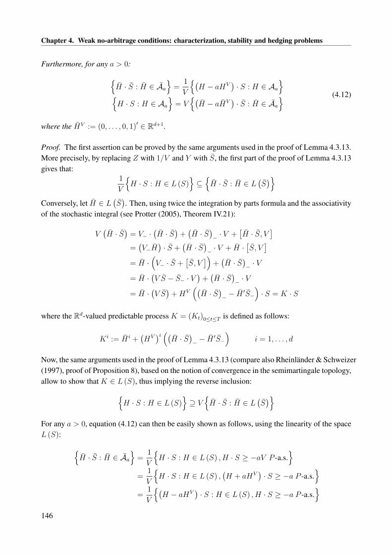
Chapter 4. Weak no-arbitrage conditions: characterization, stability and hedging problems
Furthermore, for any a > 0:H · S : H ∈ Aa
=
1
V
(H − aHV
)· S : H ∈ Aa
H · S : H ∈ Aa
= V
(H − aHV
)· S : H ∈ Aa
(4.12)
where the HV := (0, . . . , 0, 1)′ ∈ Rd+1.
Proof. The first assertion can be proved by the same arguments used in the proof of Lemma 4.3.13.More precisely, by replacing Z with 1/V and Y with S, the first part of the proof of Lemma 4.3.13gives that:
1
V
H · S : H ∈ L (S)
⊆H · S : H ∈ L
(S)
Conversely, let H ∈ L(S). Then, using twice the integration by parts formula and the associativity
of the stochastic integral (see Protter (2005), Theorem IV.21):
V(H · S
)= V− ·
(H · S
)+(H · S
)− · V +
[H · S, V
]=(V−H
)· S +
(H · S
)− · V + H ·
[S, V
]= H ·
(V− · S +
[S, V
])+(H · S
)− · V
= H ·(V S − S− · V
)+(H · S
)− · V
= H ·(V S)
+HV((H · S
)− − H
′S−
)· S = K · S
where the Rd-valued predictable process K = (Kt)0≤t≤T is defined as follows:
Ki := H i +(HV)i ((
H · S)− − H
′S−
)i = 1, . . . , d
Now, the same arguments used in the proof of Lemma 4.3.13 (compare also Rheinländer & Schweizer(1997), proof of Proposition 8), based on the notion of convergence in the semimartingale topology,allow to show that K ∈ L (S), thus implying the reverse inclusion:
H · S : H ∈ L (S)⊇ V
H · S : H ∈ L
(S)
For any a > 0, equation (4.12) can then be easily shown as follows, using the linearity of the spaceL (S):
H · S : H ∈ Aa
=1
V
H · S : H ∈ L (S) , H · S ≥ −aV P -a.s.
=
1
V
H · S : H ∈ L (S) ,
(H + aHV
)· S ≥ −a P -a.s.
=
1
V
(H − aHV
)· S : H ∈ L (S) , H · S ≥ −a P -a.s.
146

4.4 Stability properties of weak no-arbitrage conditions
Similarly, by using the representation 1V
= 1 + HV · S, where HV := (0, . . . , 0, 1)′ ∈ Rd+1, weobtain the following relation, for any a > 0:
H · S : H ∈ Aa
= VH · S : H ∈ L
(S), H · S ≥ − a
VP -a.s.
= V
H · S : H ∈ L
(S),(H + aHV
)· S ≥ −a P -a.s.
= V
(H − aHV
)· S : H ∈ L
(S), H · S ≥ −a P -a.s.
The following Theorem deals with the behavior of the No Unbounded Increasing Profit (NUIP)condition under a change of numéraire. The proof is based on some simple but lengthy computa-tions and is given in the Appendix.
Theorem 4.4.3. Let V = 1 + H · S be a numéraire for S. If S satisfies the NUIP condition, thenS admits the following canonical decomposition:
S = S0 + A+ M
where M is an Rd+1-valued continuous local martingale with M0 = 0 and A is an Rd+1-valuedcontinuous predictable process of finite variation with A0 = 0 and such that, for all t ∈ [0, T ]:
Ait =d+1∑j=1
∫ t
0
λjud⟨M i, M j
⟩u
i = 1, . . . , d+ 1 (4.13)
where λjt := Vtλjt , for all j = 1, . . . , d, and λd+1
t := Vt
(1−
∑dk=1 S
kt λ
kt
), for all t ∈ [0, T ], and
where the process λ = (λt)0≤t≤T is as in Theorem 4.3.2.Conversely, if S satisfies the NUIP condition, then the following hold for all t ∈ [0, T ]:
Ait =d∑j=1
∫ t
0
λjud〈M i,M j〉u, i = 1, . . . , d where λjt :=λjtVt
+
(1−
d+1∑k=1
Skt λkt
Vt
)Hjt
Vt, j = 1, . . . , d
whereA andM denote the finite variation and the local martingale part, respectively, in the canon-ical decomposition of the Rd-valued semimartingale S and where the process λ =
(λt)
0≤t≤T is theRd+1-valued predictable process which satisfies dA = d〈M, M〉λ.In particular, the NUIP condition holds for S if and only if the NUIP condition holds for S =(SV, 1V
).
From an economic point of view, the result of Theorem 4.4.3 is somewhat expected. In fact,as we argued in Section 4.3.1, the NUIP condition excludes only very strong (pathological) formsof arbitrage. Therefore, it is natural to conjecture that the validity of the NUIP condition shouldnot depend on the choice of the reference asset in terms of which we express all market prices. Itis worth pointing out that Theorem 4.4.3 not only shows that the NUIP condition is stable undera change of numéraire, but also gives the explicit canonical decomposition of the price process
147
Chapter 4. Weak no-arbitrage conditions: characterization, stability and hedging problems
under the new numéraire. Furthermore, we can also explicitly compute the mean-variance tradeoffprocess of S in terms of the original price process S, as shown in the following Corollary, the proofof which is given in the Appendix.
Corollary 4.4.4. Let V = 1 + H · S be a numéraire for S and suppose that S satisfies the NUIPcondition. Then the mean-variance tradeoff process K =
(Kt
)0≤t≤T for S =
(SV, 1V
)is explicitly
given as follows, for all t ∈ [0, T ]:
Kt :=d+1∑i,j=1
∫ t
0
λiuλjud〈M i, M j〉u =
∫ t
0
(Hu
Vu− λu
)′d〈M,M〉u
(Hu
Vu− λu
)(4.14)
Having shown the stability of the NUIP condition with respect to a change of numéraire, we nowmove to the No Immediate Arbitrage Opportunity (NIAO) condition, analyzed in Section 4.3.2. Thefollowing Theorem shows that also the NIAO condition is not affected by a change of numéraire.The proof of the following Theorem uses only Definition 4.3.6 and Lemma 4.4.2 and, hence, itholds true also for general (possibly discontinuous and non-locally bounded) semimartingales.
Theorem 4.4.5. Let V = 1 + H · S be a numéraire for S. Then the NIAO condition holds for S ifand only if the NIAO condition holds for S =
(SV, 1V
).
Proof. We shall argue by contradiction. Suppose first that the NIAO condition holds for S butthere exists a strategy K ∈ A0 which generates an immediate arbitrage opportunity for S, withrespect to a stopping time τ with P (τ < T ) > 0. Due to Lemma 4.4.2, there exists a strategyK ∈ L (S) such that K · S = V
(K · S
). Since K · S = 0 on the stochastic interval [[0, τ ]], we
can assume that K = K1]]τ,T ]]. On the set τ < T, we have (K · S)t = Vt(K · S
)t> 0 P -a.s.
for all t ∈ (τ, T ], since V > 0 P -a.s. Due to Definition 4.3.6, this shows that the strategy K ∈ A0
generates an immediate arbitrage opportunity for S, thus contradicting the assumption that NIAOholds for S. The converse implication can be shown in analogous way. Indeed, suppose that theNIAO condition holds for S and let K ∈ A0 generate an immediate arbitrage opportunity for S,with respect to a stopping time τ with P (τ < T ) > 0. Then, due to Lemma 4.4.1, there exists anelement K ∈ L
(S)
such that K · S = 1V
(K · S). Since K ·S = 0 on the stochastic interval [[0, τ ]],we can assume that K = K1]]τ,T ]]. On the set τ < T, we have
(K · S
)t
= 1Vt
(K · S)t > 0 P -a.s.for all t ∈ (τ, T ], since V > 0 P -a.s., which contradicts the assumption that the NIAO conditionholds for S.
Remark 4.4.6 (An alternative proof to Theorem 4.4.5). We want to point out that Theorem 4.4.5can also be proved by relying on Theorem 4.3.10 and Corollary 4.4.4. In fact, due to Corollary4.4.4 and to the Cauchy-Schwarz inequality, the mean-variance tradeoff process K for S satisfiesthe following inequalities, for all t ∈ [0, T ]:
Kt −∫ t
0
1
V 2u
H ′ud〈M,M〉uHu ≤∫ t
0
(Hu
Vu− λu
)′d〈M,M〉u
(Hu
Vu− λu
)= Kt =
∫ t
0
(Hu
Vu− λu
)′d〈M,M〉u
(Hu
Vu− λu
)≤∫ t
0
1
V 2u
H ′ud〈M,M〉uHu + Kt
(4.15)
148

4.4 Stability properties of weak no-arbitrage conditions
where the process K is as in (4.4). Due to Definition 4.4.1, we have H ∈ L (S) ⊆ L2loc (M),
thus implying that∫ t
01V 2uH ′ud〈M,M〉uHu < ∞ P -a.s. for all t ∈ [0, T ], since the process 1/V is
continuous and, hence, locally bounded. Thus, as can be seen from (4.15), we have that the processK jumps to infinity if and only if the process K jumps to infinity. Due to Theorem 4.3.10, thismeans that the NIAO condition holds for S if and only if the NIAO condition holds for S.
Let us now study the behavior of the crucial No Unbounded Profit with Bounded Risk (NUPBR)condition under a change of numéraire. The proof of the following Theorem is surprisingly simpleand follows easily from Lemma 4.4.2. As for Theorem 4.4.5, observe that the proof of the followingTheorem does not rely on the continuity of the semimartingale S. Hence, the result of Theorem4.4.7 holds true also in financial market models based on general (possibly discontinuous and non-locally bounded) semimartingales.
Theorem 4.4.7. Let V = 1 +H · S be a numéraire for S. Then the NUPBR condition holds for Sif and only if the NUPBR condition holds for S.
Proof. The second part of Lemma 4.4.2, for a = 1, implies that:(H · S)T : H ∈ A1
= VT
(H · S
)T
: H ∈ A1
− VT
(HV · S
)T
= VT
(H · S
)T
: H ∈ A1
− 1 + VT
where the second equality uses the fact that 1V
= 1 + HV · S and the fact that L(S)
is a linearspace. Since the random variable VT is finite and P -a.s. strictly positive and since boundednessin probability is not affected by the multiplication and the addition of VT , this shows that theset (H · S)T : H ∈ A1 is bounded in probability if and only if the set
(H · S
)T
: H ∈ A1
is
bounded in probability.
We want to point out that the necessity part of Theorem 4.4.7 has been shown also in the recentpaper Takaoka (2010). Furthermore, the result of Theorem 4.4.7 can be also obtained by combiningour Theorem 4.3.23 with Corollary 2.8 of Choulli & Stricker (1996). However, the continuity of Sis essential in the proof of Corollary 2.8 of Choulli & Stricker (1996), unlike the simple proof ofTheorem 4.4.7 here provided.
Remark 4.4.8 (An alternative proof to Theorem 4.4.7). Similarly as in Remark 4.4.6, we canalso give an alternative proof of Theorem 4.4.7 by relying on Theorem 4.3.23 and Corollary 4.4.4.In fact, equation (4.15) shows that we have KT < ∞ P -a.s. if and only if KT < ∞ P -a.s. Dueto Theorem 4.3.23, this means that the NUPBR condition holds for S if and only if the NUPBRcondition holds for S. For a related result on the finiteness of the mean-variance tradeoff processunder a change of numéraire, see also Lemma 4.5 of Delbaen & Shirakawa (1996).
Summing up, Theorems 4.4.3, 4.4.5 and 4.4.7 together show that all the weak no-arbitrageconditions considered in Section 4.3 are stable with respect to a change of numéraire. As we alreadyargued above, the robustness with respect to the choice of the numéraire should be regarded froman economic point of view as a fundamental property of a no-arbitrage condition.
149
Chapter 4. Weak no-arbitrage conditions: characterization, stability and hedging problems
Let us close this Section by comparing the stability properties of the weak no-arbitrage condi-tions discussed so far with the stability properties (or the lack thereof) of the classical No Arbitrage(NA) and No Free Lunch with Vanishing Risk (NFLVR) conditions. In Delbaen & Schachermayer(1995c), the authors study the impact of a change of numéraire on the classical NA and NFLVR con-ditions, showing that the NA condition (and hence, recalling part (a) of Proposition 4.3.28, also theNFLVR condition) is not necessarily stable with respect to a change of numéraire. More precisely(see Delbaen & Schachermayer (1995c), Theorem 4.4), assuming that the NFLVR condition holdsfor S, the NA condition (and, hence, in view of part (a) of Proposition 4.3.28 and Theorem 4.4.7,also the NFLVR condition) holds for S if and only if there exists a probability measureQ on (Ω,F)
with Q ∼ P such that S is a local Q-martingale and V is a uniformly integrable Q-martingale, i.e.an ELMM Q for S such that the numéraire process is a uniformly integrable Q-martingale. Itfollows that the NA condition is not necessarily preserved by a change of numéraire. For a sim-ple counterexample, we refer the interested reader to Example 4.1 in Delbaen & Schachermayer(1995c). In a nutshell, the reason why the NA condition is not stable under a change of numéraireis due to the definition of admissible strategy (see Definition 4.2.2). Indeed, it could be that thereis arbitrage with respect to S =
(SV, 1V
)but the NA condition still holds for S, since the strategy
which realizes the arbitrage with respect to S is not admissible for S because it fails to be lowerbounded by some constant. From an economic point of view, the fact that the NA and NFLVRconditions are affected by the choice of the reference numéraire represents a significant drawbackof the classical no-arbitrage theory based on NA and NFLVR.
4.4.2 Absolutely continuous changes of measure
This Section continues the study of the robustness properties of the weak no-arbitrage conditionsdiscussed in Section 4.3. More specifically, in the present Section we shall be concerned withthe stability of the NUIP/NIAO/NUPBR conditions under an absolutely continuous change of thereference probability measure. Recall that we started in Section 4.2 by considering an abstractfinancial market model formulated with respect to a fixed probability measure P on (Ω,F). Let usnow suppose that one of the NUIP/NIAO/NUPBR conditions holds with respect to P and consideranother probability measure Q on (Ω,F) with Q P . We can then ask the following question.Does the NUIP/NIAO/NUPBR condition still holds with respect to Q? What about the classicalNA and NFLVR conditions? In this Section, we shall provide an answer to these questions.
Let Q be a given probability measure on (Ω,F) with Q P and denote by ZQ =(ZQt
)0≤t≤T
its density process with respect to P , i.e. ZQt = E
[dQdP|Ft]
for all t ∈ [0, T ]. Recall that ZQ is a uni-formly integrable P -martingale, which also satisfiesQ
(ZQt > 0 and ZQ
t− > 0 for all t ∈ [0, T ])
= 1
(see e.g. Revuz & Yor (1999), Proposition VIII.1.2). Note that the P -martingale ZQ is not nec-essarily continuous. Recall also that S is supposed to be an Rd-valued continuous semimartingaleon the filtered probability space (Ω,F ,F, P ). Hence, due to Theorem II.2 of Protter (2005), theprocess S is also a semimartingale with respect to the probability measure Q. Furthermore, due tothe Girsanov-Lenglart Theorem for absolutely continuous changes of measure (see Protter (2005),Theorem III.41), we can compute the canonical decomposition of S with respect to Q, as shown in
150

4.4 Stability properties of weak no-arbitrage conditions
the following Lemma.
Lemma 4.4.9. Let Q be a probability measure on (Ω,F) with Q P . Then the density processZQ of Q with respect to P can be represented as follows:
ZQ = ZQ0 + θ ·M +N (4.16)
for some Rd-valued predictable process θ = (θt)0≤t≤T in L2loc (M) and for some real-valued local
martingale N = (Nt)0≤t≤T strongly orthogonal to M with N0 = 0. Moreover, the Rd-valuedcontinuous semimartingale S admits the canonical decomposition S = S0 +AQ+MQ with respectto Q, where AQ in an Rd-valued continuous predictable process of finite variation with AQ0 = 0
and MQ is an Rd-valued continuous local martingale with MQ0 = 0, explicitly given as follows:
AQ = A+
∫1
ZQ−d〈M,M〉θ and MQ = M −
∫1
ZQ−d〈M,M〉θ (4.17)
whereA andM denote the finite variation and the local martingale part, respectively, in the canon-ical decomposition of S with respect to P .
Proof. Equation (4.16) represents the Galtchouk-Kunita-Watanabe decomposition of the (uniformlyintegrable) martingale ZQ with respect to the continuous local martingale M , see Ansel & Stricker(1993). Then, Theorem III.41 of Protter (2005) implies that the process MQ =
(MQ
t
)0≤t≤T de-
fined by MQt := Mt−
∫ t0
1
ZQu−d〈M,ZQ〉u is a local Q-martingale. Note that, since M is continuous,
the predictable quadratic variation 〈M,ZQ〉 always exists. Hence, we get the following canonicaldecomposition of S with respect to Q:
S = S0 +
(A+
∫1
ZQ−d〈M,ZQ〉
)+
(M −
∫1
ZQ−d〈M,ZQ〉
)The expressions in (4.17) then follow from (4.16), using also the fact that 〈M,N〉 ≡ 0 due to thecontinuity of M and to the strong orthogonality of M and N .
By relying on the above Lemma, we can easily prove the stability of the NUIP condition withrespect to an absolutely continuous change of the reference probability measure.
Theorem 4.4.10. Let Q be a probability measure on (Ω,F) with Q P and suppose that theNUIP condition holds with respect to P . Then the NUIP condition holds with respect to Q as well.
Proof. Suppose that the NUIP condition holds with respect to P . Then, due to Theorem 4.3.2,there exists an Rd-valued predictable process λ = (λt)0≤t≤T such that dA = d〈M,M〉λ. Hence, ifQ is a probability measure on (Ω,F) with Q P , Lemma 4.4.9 implies the following:
AQ = A+
∫1
ZQ−〈M,M〉θ =
∫d〈M,M〉
(λ+
θ
ZQ−
)=
∫d〈MQ,MQ〉
(λ+
θ
ZQ−
)(4.18)
where we have also used the fact that 〈M,M〉 = 〈MQ,MQ〉. This shows that dAQ=d〈MQ,MQ〉λQ,where the Rd-valued predictable process λQ =
(λQt)
0≤t≤T is given by λQ := λ + θ
ZQ−. Theorem
4.3.2 then implies that the NUIP condition holds with respect to Q as well.
151

Chapter 4. Weak no-arbitrage conditions: characterization, stability and hedging problems
In order to study the stability of the NIAO and NUPBR conditions under an absolutely continu-ous change of measure, let us first compute the mean-variance tradeoff process KQ =
(KQt
)0≤t≤T
of S with respect to the probability measure Q.
Lemma 4.4.11. Let Q be a probability measure on (Ω,F) with Q P . Then the mean-variancetradeoff process KQ =
(KQt
)0≤t≤T of S with respect to the probability measure Q is explicitly
given as follows, for all t ∈ [0, T ]:
KQt :=
d∑i,j=1
∫ t
0
(λQu)i (
λQu)jd⟨(MQ
)i,(MQ
)j⟩u
=
∫ (λ+
θ
ZQ−
)′d〈M,M〉
(λ+
θ
ZQ−
)(4.19)
Furthermore, the process KQ satisfies the following inequality, for all t ∈ [0, T ]:
KQt ≤ Kt +
∫ t
0
1(ZQu−)2 θ
′ud〈M,M〉uθu (4.20)
Proof. Equation (4.19) follows directly from equation (4.18), using the fact that 〈M,M〉=〈MQ,MQ〉.Equation (4.20) is then a simple consequence of the Cauchy-Schwarz inequality together with(4.4).
We can now easily prove the following Theorem, which shows the stability of the NIAO andNUPBR conditions with respect to an absolutely continuous change of the reference probabilitymeasure.
Theorem 4.4.12. Let Q be a probability measure on (Ω,F) with Q P . If the NIAO conditionholds with respect to P then it holds with respect to Q as well. In addition, if the NUPBR conditionholds with respect to P then it holds with respect to Q as well.
Proof. Suppose first that the NIAO condition holds with respect to P . As pointed out in Section4.3.2, the NIAO condition implies the NUIP condition and Theorem 4.4.10 shows that the NUIPcondition holds with respect to Q. In particular, there exists an Rd-valued predictable processλQ =
(λQt)
0≤t≤T such that dAQ = d〈MQ,MQ〉λQ. Hence, in view of Theorem 4.3.10, to showthat the NIAO condition holds with respect to Q it suffices to show that the mean-variance tradeoffprocess KQ defined in (4.19) does not jump to infinityQ-a.s. Since the NIAO condition holds underP , Theorem 4.3.2 implies that α := inf
t > 0 : Kt+h
t = ∞,∀h ∈ (0, T − t]
= ∞ P -a.s. andalso Q-a.s., since Q P . Note that the second term in the right hand side of (4.20) is continuousand P -a.s. (and, hence, also Q-a.s.) finite, because θ ∈ L2
loc (M) and the process 1/ZQ− is locally
bounded, being left-continuous. Due to the inequality (4.20), this implies the following:
αQ := inft > 0 : KQ
t+h − KQt =∞,∀h ∈ (0, T − t]
= α =∞ Q-a.s.
Due to Theorem 4.3.10, we can conclude that the NIAO condition holds with respect toQ. Supposenow that the NUPBR condition holds with respect to P . In view of Theorem 4.3.23, since theNUPBR condition is stronger than the NUIP/NIAO conditions and since we already know that the
152

4.4 Stability properties of weak no-arbitrage conditions
latter hold under Q, to show that NUPBR holds with respect to Q it suffices to show that KQT <∞
Q-a.s. Since NUPBR holds under P , Theorem 4.3.23 implies that KT <∞ P -a.s. and also Q-a.s.,since Q P . Thus, equation (4.20) gives KQ
T < ∞ Q-a.s. Due to Theorem 4.3.23, we canconclude that the NUPBR condition holds with respect to Q.
Summing up, Theorems 4.4.10 and 4.4.12 show that the weak no-arbitrage conditions consid-ered in Section 4.3 are all stable with respect to an absolutely continuous change of the referenceprobability measure. However, this stability property is not enjoyed by the classical No Arbitrage(NA) and No Free Lunch with Vanishing Risk (NFLVR) conditions, as we are going to show in thenext Example, which is based on Delbaen & Schachermayer (1995a).
Example 4.4.13. Let W = (Wt)0≤t≤T be a standard Brownian motion starting from W0 = 1 anddefine the stopping time τ := inf t ∈ [0, T ] : Wt = 0∧T . We define the discounted price processS of a single risky asset as the stopped process S := W τ and we assume that the filtration F is theP -augmented natural filtration of S, with F = FT . Clearly, the process S is a martingale. Hence,recalling Proposition 4.3.28, the NA and NFLVR no-arbitrage conditions hold with respect to P .Let us also define a probability measure Q on (Ω,F) by letting dQ
dP:= ST = WT∧τ = Wτ . Clearly,
we have Q P but P Q does not hold, meaning that the probability measures Q and P are notequivalent. Observe that the process S represents also the density process of Q with respect to P .In fact, for all t ∈ [0, T ]:
E
[dQ
dP
∣∣∣Ft] = E [ST |Ft] = E [Wτ |Ft] = Wt∧τ = St
By the Girsanov-Lenglart Theorem for absolutely continuous changes of measure (see Protter(2005), Theorem III.41), the process N = (Nt)0≤t≤T defined by N := S −
∫1Sd〈S, S〉 is a con-
tinuous local Q-martingale. Note that 〈N,N〉t = 〈S, S〉t = t ∧ τ for all t ∈ [0, T ]. Furthermore,since Q (ST = 0) = E
[1ST=0ST
]= 0, so that τ = T Q-a.s., we have 〈N,N〉t = t Q-a.s.
for all t ∈ [0, T ]. Lévy’s characterization of Brownian motion (see e.g. Protter (2005), TheoremII.39) implies then that N is a Q-Brownian motion starting at N0 = 1. Let us denote by G the Q-augmented natural filtration of N (or, equivalently, of S). It can be easily seen that the filtration Gcoincides with F augmented by the subsets of ST = 0. We now show that S does not satisfy theNA condition on the filtered probability space (Ω,G,G, Q), with G = GT . Indeed, suppose on thecontrary that S satisfies the NA condition on (Ω,G,G, Q). Then, due to Theorem 4.4.12 togetherwith Proposition 4.3.28, there exists a probability measure Q′ on (Ω,G) with Q′ ∼ Q such that Sis a local Q′-martingale. Let us denote by ZQ′ the density process of Q′ with respect to Q. The(Q,G)-Brownian motion N enjoys the representation property, since G is its Q-augmented naturalfiltration. Hence, due to Corollary 2 to Theorem IV.43 of Protter (2005), we have the representationZQ′ = E (−θ ·N), for some G-predictable process θ = (θt)0≤t≤T such that
∫ T0θ2t dt < ∞ Q-a.s.
Let us compute the stochastic differential of the product ZQ′S:
d(ZQ′
t St)
= ZQ′
t dSt + StdZQ′
t + d〈ZQ′ , S〉t = ZQ′
t dNt +ZQ′
t
Stdt− ZQ′
t StθtdNt − ZQ′
t θtdt
153

Chapter 4. Weak no-arbitrage conditions: characterization, stability and hedging problems
Since ZQ′S is a local Q-martingale and ZQ′ > 0 Q-a.s., this implies that θt = 1StQ-a.s. for all
t ∈ [0, T ], thus yielding ZQ′ = E(− 1S·N). Equivalently, the process ZQ′ =
(ZQ′
t
)0≤t≤T is the
unique solution to the following SDE:
dZQ′
t = −ZQ′
t
1
StdNt ZQ′
0 = 1 (4.21)
On the other hand, Itô’s formula gives the following:
d1
St= − 1
S2t
dSt +1
S3t
d〈S〉t = − 1
S2t
dNt −1
S3t
dt+1
S3t
dt = − 1
S2t
dNt1
S0
= 1 (4.22)
Equations (4.21)-(4.22) show that the processes ZQ′ =(ZQ′
t
)0≤t≤T and 1/S =
(1/St
)0≤t≤T solve
the same SDE with the same initial condition and, hence, we must have ZQ′
t = 1StQ-a.s. for all
t ∈ [0, T ]. At this point, observe that the process S = (St)0≤t≤T , which satisfies dSt = dNt + 1Stdt
with respect to the (Q,G)-Brownian motion N , is a Bessel process of dimension three (see Revuz& Yor (1999), Section XI.1). It is well-known that the reciprocal of a 3-dimensional Bessel processis a strict local martingale, i.e. a local martingale which is not a true martingale (see e.g. Revuz& Yor (1999), Exercise XI.1.16). This implies that the process ZQ′ cannot be a true martingale,thus contradicting the existence of the measure Q′. Due to part (c) of Proposition 4.3.28, thisimplies that the NFLVR condition does not hold on (Ω,G,G, Q). On the other hand, observe thatthe process ZQ′ is a martingale deflator for S on (Ω,G,G, Q), so that, due to Theorem 4.3.23,the NUPBR condition holds. Hence, part (a) of Proposition 4.3.28 implies that the NA conditionfails on (Ω,G,G, Q). So, there exists a G-predictable S-integrable (with respect to (Q,G)) processH = (Ht)0≤t≤T with G (H) ≥ −a Q-a.s., for some a ∈ R+, and such that GT (H) ≥ 0 Q-a.s. andQ(GT (H) > 0
)> 0. As pointed out on page 360 of Delbaen & Schachermayer (1995a), there
also exists an F-predictable process K = (Kt)0≤t≤T which is Q-indistinguishable from H , so thatK ·S = H ·S, where both stochastic integrals are considered with respect to (Q,G). Since S andKare both F-predictable, Theorem 7 of Jacod (1980) shows that the stochastic integral K · S viewedwith respect to (Q,G) is the same as the stochastic integral viewed with respect to (Q,F). Thismeans that the F-predictable process K = (Kt)0≤t≤T is integrable with respect to S (with respectto (Q,F)) and satisfies G (K) ≥ −a Q-a.s. and GT (K) ≥ 0 Q-a.s. and Q
(GT (K) > 0
)> 0.
Hence, we can conclude that the NA condition fails on (Ω,F ,F, Q), thus finishing the Example.
Remark 4.4.14 (On equivalent changes of measure). We close this Section by pointing out that,if we consider an equivalent change of measure, rather than an absolutely continuous change ofmeasure, then the NA and NFLVR conditions are also preserved. Indeed, suppose that the NAcondition holds with respect to P and let Q be a probability measure on (Ω,F) with Q ∼ P .Arguing by contradiction, suppose that there exists an Rd-valued predictable S-integrable (withrespect to Q) process H = (Ht)0≤t≤T with G (H) ≥ −a Q-a.s., for some a ∈ R+, and suchthat GT (H) ≥ 0 Q-a.s. and Q
(GT (H) > 0
)> 0. Then, since Q ∼ P , Theorem IV.25 of
Protter (2005) shows that the process H is also S-integrable with respect to P and the stochasticintegral H · S viewed with respect to P coincides with the stochastic integral H · S viewed withrespect to Q. Since Q ∼ P , we also have G (H) ≥ −a P -a.s. and GT (H) ≥ 0 P -a.s. and
154

4.4 Stability properties of weak no-arbitrage conditions
P(GT (H) > 0
)> 0. Clearly, this contradicts the assumption that the NA condition holds with
respect to P , thus showing that an equivalent change of measure does not affect the validity of theNA condition. Due to part (a) of Proposition 4.3.28 together with Theorem 4.4.12, the same holdstrue for the NFLVR condition.
4.4.3 Changes of the reference filtration
In this Section we shall be concerned with the issue of the robustness of the weak no-arbitrageconditions analyzed in Section 4.3 with respect to changes in the reference filtration. Intuitively,this amounts to study the impact on the weak no-arbitrage conditions of restrictions/enlargementsof the information set available to market participants. This study is not only of theoretical interestbut has also important implications from an economic point of view. Indeed, it allows to show in arigorous way the relation between the possibility of making arbitrages (in a suitable sense) and thequality of the information available to the investors. Furthermore, these issues are also connectedto the analysis of economically relevant situations like insider trading and partial information. InSection 4.4.3 we shall consider the case where the information set is restricted, while Section 4.4.3will be devoted to the analysis of the case where the information set is expanded.
Restriction of the filtration
We continue to work within the general framework described in Section 4.2 and we let S be anRd-valued continuous semimartingale on the filtered probability space (Ω,F ,F, P ) with canonicaldecomposition S = S0 + A + M . Furthermore, we let E = (Et)0≤t≤T be a filtration satisfying theusual conditions on the probability space (Ω,F , P ) and such that E ⊆ F, meaning that Et ⊆ Ftfor all t ∈ [0, T ]. We also assume that the F-semimartingale S is E-adapted. The basic questionwe shall answer in this Section can be formulated in the following terms. Suppose that one of theNUIP/NIAO/NUPBR no-arbitrage conditions holds on the filtered probability space (Ω,F ,F, P ).Does the same no-arbitrage condition hold with respect to (Ω,F ,E, P ) as well? In other words:does the restriction of the information set affect the no-arbitrage condition? Our intuition suggeststhat, if there is no-arbitrage (in a suitable sense) in the original full-information financial market(i.e. with respect to F) and we restrict the information set available to market participants, thenarbitrage should not be possible in the restricted information financial market (i.e. with respect toE) as well. As will be shown below, this conjecture is indeed valid and can be rigorously justified.
As a preliminary, recall that S is a continuous (and, hence, special) F-semimartingale, withcanonical decomposition S = S0 + A + M , where A is an Rd-valued continuous F-predictableprocess of finite variation with A0 = 0 and M is an Rd-valued continuous F-local martingale withM0 = 0. Since E ⊆ F and S is supposed to be E-adapted, Stricker’s Theorem (see Protter (2005),Theorem II.4) implies that S is also a special E-semimartingale and we denote by S = S0 + A+M
its canonical decomposition with respect to E, where A is an Rd-valued continuous E-predictableprocess of finite variation with A0 = 0 and M is an Rd-valued continuous E-local martingale withM0 = 0. Furthermore, we denote by L (S,F) the set of all Rd-valued F-predictable S-integrable
155

Chapter 4. Weak no-arbitrage conditions: characterization, stability and hedging problems
(with respect to the filtration F) processes and, analogously, we denote by L (S,E) the set of allRd-valued E-predictable S-integrable (with respect to the filtration E) processes.
At this point, note that it is tempting to answer the questions formulated at the beginning ofthis Section by relying on the following reasoning. Suppose the one of the NUIP/NIAO/NUPBRconditions holds with respect to the filtration F and let H = (Ht)0≤t≤T be an element of L (S,E)
which realizes an arbitrage (in the sense of UIP/IAO/UPBR, respectively) in the filtration E. Then,since E ⊆ F, the process H is also F-predictable and, hence, can be viewed as a trading strategyin the filtration F (in plain words, nothing should prevent a more informed trader from neglectingpart of the information available to her). Hence, one is led to conjecture that L (S,E) ⊆ L (S,F),so that the strategy H , now viewed with respect to the filtration F, yields an arbitrage (in the senseof UIP/IAO/UPBR, respectively) also in the filtration F, thus contradicting the assumption thatNUIP/NIAO/NUPBR holds with respect to the filtration F. Hence, one would conclude that theNUIP/NIAO/NUPBR conditions are stable with respect to a restriction of the reference filtration.The flaw in this line of reasoning is that the inclusion L (S,E) ⊆ L (S,F) is not true in general,as shown by an explicit counterexample in Chou et al. (1980) (see also Jeulin (1980), Theorem3.23). The inclusion holds true if we restrict our attention to locally bounded integrands, as shownin Theorem 9.19 of Jacod (1979) and in Theorem IV.33 of Protter (2005). However, as pointed outin Remark 4.2.1, we have chosen to work with the most general class of integrands, which includesnon-locally bounded processes. Hence, the above reasoning fails and special care must be taken.
The following Theorem studies the impact of a restriction of the reference filtration on the NoUnbounded Increasing Profit (NUIP) condition. Furthermore, it gives a characterization of thefinite variation part A in the canonical decomposition of S with respect to the filtration E.
Theorem 4.4.15. Let E be a filtration with E ⊆ F and suppose that S is E-adapted. If the NUIPcondition holds with respect to F then it holds with respect to E as well. Furthermore, the finitevariation part A in the canonical decomposition of S with respect to E can be represented asfollows, for all t ∈ [0, T ]:
Ait =
∫ t
0
d〈M i, M〉u (p,E)λu i = 1, . . . , d
where M is the local martingale part in the canonical decomposition of S with respect to E and(p,E)λ denotes the E-predictable projection of the process λ, the latter being as in Theorem 4.3.2.
Proof. Note first that we have 〈M,M〉 = 〈S, S〉 = 〈M, M〉 and 〈S, S〉 does not depend on thechoice of the reference filtration. Indeed, due to the continuity of S, we have 〈S, S〉 = [S, S] andthe latter does not depend on the reference filtration, being the limit (in probability) of the pathwisequadratic variation of S (compare also Jacod (1979), part (b) of Theorem 9.19) For every n ∈ N,let us define the E-stopping time τn as follows:
τn := inf
t ∈ [0, T ] : ‖St − S0‖ ≥ n or
d∑i,j=1
〈Si, Sj〉t ≥ n
∧ T
156

4.4 Stability properties of weak no-arbitrage conditions
Clearly, since both S and 〈S, S〉 are P -a.s. finite valued, we have τn T P -a.s. as n → ∞. Forevery n ∈ N, the stopped process 〈M,M〉τn = 〈M τn ,M τn〉 is bounded and, hence, the F-localmartingale M τn is an Rd-valued uniformly integrable F-martingale. Similarly, the same holds truefor the stopped process M τn , for every n ∈ N, with respect to the filtration E. Note that, for everyn ∈ N, we have Aτn = Sτn − S0 −M τn ≤ n −M τn and, hence, Aτnt ∈ L1 (P ) for all t ∈ [0, T ].Similarly, the same holds true for the stopped process Aτn , for every n ∈ N, with respect to thefiltration E. So, for any E-stopping time τ and for every n ∈ N:
E [Aτnτ ] = E [Sτnτ − S0]− E [M τnτ ] = E [Sτnτ − S0] = E [Sτnτ − S0]− E
[M τn
τ
]= E
[Aτnτ]
where the second and the third equalities follow from the optional sampling theorem (see e.g.Protter (2005), Theorem I.16) together with the uniform integrability ofM τn and M τn , respectively.Due to Theorem 9.22 of Jacod (1979), we can conclude that Aτn is the dual predictable projectionof Aτn with respect to E, i.e. Aτn = (Aτn)(p,E), for every n ∈ N. Furthermore, the following holds:
Aτn = (Aτn)(p,E) =(1[[0,τn]] · A
)(p,E)= 1[[0,τn]] · A(p,E) =
(A(p,E)
)τnwhere the third equality follows from 9.23 of Jacod (1979), since τn is an E-stopping time for alln ∈ N. Since τn T P -a.s. as n → ∞, this shows that A = A(p,E) (see also Jacod (1979),Proposition 9.24). Suppose now that the NUIP condition holds with respect to F. Then, due toTheorem 4.3.2, there exists an Rd-valued F-predictable process λ = (λt)0≤t≤T such that dA =
d〈M,M〉λ. We can thus write the following (compare also with Kohlmann et al. (2007), Lemma2.2):
A = A(p,E) =
(∫d〈M,M〉λ
)(p,E)
=
(∫d〈M, M〉λ
)(p,E)
=
∫d〈M, M〉 (p,E)λ
where the last equality follows from 9.23 of Jacod (1979) and (p,E)λ denotes the predictable projec-tion of λ with respect to the filtration E. Due to Theorem 4.3.2, this shows that the NUIP conditionholds with respect to the filtration E as well.
Theorem 4.4.15 shows that, if the continuous E-adapted F-semimartingale S satisfies the NUIPcondition with respect to the filtration F, then it satisfies the NUIP condition with respect to thefiltration E as well. Note that the proof of Theorem 4.4.15 makes use of the continuity of thesemimartingale S. Our next goal consists in showing that the same result holds true also in the casewhere S is a general (possibly discontinuous and non-locally bounded) semimartingale, providedwe make the following natural assumption concerning the structure of the filtrations E and F.
Assumption 4.4.16. Every E-semimartingale is also an F-semimartingale.
Remark 4.4.17. In the theory of enlargement of filtrations, Assumption 4.4.16 is commonly knownas the (H ′)-hypothesis, see e.g. Chapter II of Jeulin (1980), where the interested reader can alsofind necessary and sufficient conditions for its validity (simpler results can also be found in Jacod(1979), Proposition 9.32). Observe that Assumption 4.4.16 automatically holds if one assumes the
157
Chapter 4. Weak no-arbitrage conditions: characterization, stability and hedging problems
stronger (H)-hypothesis, i.e. if every E-local martingale is also an F-local martingale, see e.g.Proposition 9.28 of Jacod (1979). However, there are situations where Assumption 4.4.16 holdsbut the (H)-hypothesis fails, see for instance part 2 of Remark 9.37 in Jacod (1979).
As soon as Assumption 4.4.16 holds, we are able to prove the following technical result, wherewe also allow the process S to be a general (possibly discontinuous and non-locally bounded)semimartingale.
Proposition 4.4.18. Let E be a filtration with E ⊆ F and assume that the Rd-valued (general) F-semimartingale S is E-adapted. Suppose that Assumption 4.4.16 holds. Then we have L (S,E) ⊆L (S,F).
Proof. The claim can be proved by relying on arguments similar to those used in the proofs ofTheorem 7 of Jacod (1980) and Theorem III.6.19 of Jacod & Shiryaev (2003). Suppose that H ∈L (S,E). Clearly, since E ⊆ F, the processH is F-predictable, being E-predictable. Let Y := H ·S,where the stochastic integral is viewed with respect to E, and define the set D := |∆S| > 1 ∪|∆Y | > 1 ⊂ Ω× [0, T ]. The optional set D is discrete, meaning that for all (ω, t) ∈ Ω× [0, T ],the set s ∈ [0, t] : (ω, s) ∈ D is finite. Therefore, we can define the processes SD =
(SDt)
0≤t≤T
and Y D =(Y Dt
)0≤t≤T as follows, for t ∈ [0, T ]:
SDt := S0 +∑s≤t
∆Ss1D (s) Y Dt :=
∑s≤t
∆Ys1D (s)
Since D is discrete we obviously have H ∈ L(SD,E
)and H · SD = Y D. Clearly, the stochastic
integral H · SD is a Stieltjes integral and, as such, does not depend on the choice of the referencefiltration. Hence, we also have H ∈ L
(SD,F
). Let us define SD := S − SD. Then, to show
that H ∈ L (S,F), it suffices to show that H ∈ L(SD,F
). In fact, due to part (d) of Theorem
III.6.19 of Jacod & Shiryaev (2003), if we have H ∈ L(SD,F
)∩ L
(SD,F
), then we also have
H ∈ L(SD + SD,F
)= L (S,F). To show that H ∈ L
(SD,F
), let us define the following
processes, for every n ∈ N:
Fn := 1‖H‖≤n H (n) := H1Fn Y D (n) := 1Fn · Y D = H (n) · SD
where Y D := Y − Y D and the stochastic integrals are viewed with respect to E. Note that theprocess Y D is a special E-semimartingale, since it has bounded jumps. Hence, due to Assumption4.4.16, it is also a special F-semimartingale, thus implying that the stochastic integral Y D (n) =
1Fn · Y D is also well-defined with respect to F. On the other hand, note that we have H (n) ∈L(SD,F
)∩ L
(SD,E
), for every n ∈ N, since H (n) is a bounded E-predictable (and, hence, also
F-predictable) process. Furthermore, due to part (c) of Theorem 9.19 of Jacod (1979), there existsa common version (i.e. with respect to both E and F) of the stochastic integralH (n) ·SD, for everyn ∈ N. This implies that we have, for every n ∈ N:
H (n) · SD = 1Fn · Y D (4.23)
158
4.4 Stability properties of weak no-arbitrage conditions
where both stochastic integrals are viewed with respect to F. Let us now denote by Y D = ND+CD
the canonical decomposition of Y D with respect to F, where ND is an F-locally square-integrableF-local martingale with ND
0 = 0 and CD is an F-predictable process of finite variation with CD0 =
0. Analogously, let us denote by SD = MD +AD the canonical decomposition of SD with respectto F, where MD is an Rd-valued F-locally square-integrable F-local martingale with MD
0 = 0 andAD is an Rd-valued F-predictable process of finite variation with AD0 = 0. Now, (4.23), togetherwith Proposition 2 of Jacod (1980), implies that, for every n ∈ N:
H (n) ·MD = 1Fn ·ND H (n) · AD = 1Fn · CD
As in Section 4.2, let B be a real-valued F-predictable increasing process of F-locally integrablevariation such thatAD =
∫adB and 〈MD,MD〉 =
∫cdB, where a and c are suitable F-predictable
processes taking values in Rd and Rd×d, respectively. Then, for every n ∈ N and t ∈ [0, T ]:((d∑
i,j=1
H icijHj
)1Fn ·B
)t
=
((d∑
i,j=1
H i (n) cijHj (n)
)·B
)t
=⟨H (n) ·MD, H (n) ·MD
⟩t
=(1Fn · 〈ND, ND〉
)t<∞ P -a.s.
Letting n→∞, we get (for t = T ):
d∑i,j=1
∫ T
0
H itcijt H
jt dBt = 〈ND, ND〉T <∞ P -a.s.
This shows that H ∈ L2loc
(MD,F
). Analogously, for every n ∈ N and t ∈ [0, T ]:((
1Fn
∣∣∣∣ d∑i=1
H iai∣∣∣∣)·B
)t
=
(∣∣∣∣ d∑i=1
H i (n) ai∣∣∣∣·B)t
=Var(H (n)·AD
)t=(1Fn·Var
(CD))
t<∞ P -a.s.
where Var denotes the total variation. Letting n→∞, we get (for t = T ):∫ T
0
∣∣∣∣ d∑i=1
H itait
∣∣∣∣dBt = Var(CD)t<∞ P -a.s.
This shows that H ∈ L0(AD,F
). Summing up, we have proved the following:
H ∈ L2loc
(MD,F
)∩ L0
(AD,F
)= L
(SD,F
)thus completing the proof of the Proposition.
Remark 4.4.19.
1. As can be seen by inspecting the proof of Proposition 4.4.18, we can actually replace As-sumption 4.4.16 with the weaker assumption that every E-semimartingale X such that X =
H · S, for some H ∈ L (S,E), is also an F-semimartingale.
159

Chapter 4. Weak no-arbitrage conditions: characterization, stability and hedging problems
2. Suppose that the stronger (H)-hypothesis (see Remark 4.4.17) holds. Then the proof ofProposition 4.4.18 can be substantially simplified. Indeed, let H ∈ L (S,E). According toDefinition III.6.17 of Jacod & Shiryaev (2003), there exists a decomposition S = S0 +B+N
of S with respect to E, withB an Rd-valued E-adapted process of finite variation withB0 = 0
and N an Rd-valued E-locally square-integrable E-local martingale with N0 = 0, such thatH ∈ L2
loc (N,E) ∩ L0 (B,E). Since E ⊆ F and every E-local martingale is also an F-localmartingale, due to the (H)-hypothesis, the decomposition S = S0 + B + N can also beviewed with respect to the larger filtration F. Clearly, the process H is F-predictable, beingE-predictable, and, hence, we have H ∈ L2
loc (N,F)∩L0 (B,F). Definition III.6.17 of Jacod& Shiryaev (2003) then implies that H is S-integrable with respect to the filtration F as well,thus showing that L (S,E) ⊆ L (S,F).
We can now state the following Corollary, the proof of which relies on Proposition 4.4.18. Inparticular, note that the result of Corollary 4.4.20 holds true also for financial market models basedon general (possibly discontinuous and non-locally bounded) semimartingales.
Corollary 4.4.20. Let E be a filtration with E ⊆ F and assume that the Rd-valued (general) F-semimartingale S is E-adapted. Suppose that Assumption 4.4.16 holds. Then the following hold:
(a) if the NUIP condition holds with respect to F then it holds with respect to E as well;
(b) if the NIAO condition holds with respect to F then it holds with respect to E as well;
(c) if the NUPBR condition holds with respect to F then it holds with respect to E as well;
(d) if the NA condition holds with respect to F then it holds with respect to E as well;
(e) if the NFLVR condition holds with respect to F then it holds with respect to E as well.
Proof. Part (a) directly follows from Definition 4.3.1 and Proposition 4.4.18, since the only prop-erty in Definition 4.3.1 that depends on the choice of the reference filtration is related to the S-integrability of the strategy generating the unbounded increasing profit. To show part (b), supposethat the NIAO condition holds with respect to F and let H = (Ht)0≤t≤T generate an immediatearbitrage opportunity with respect to E. Due to Definition 4.3.6, this means that H is an element ofL (S,E) such that H = H1]]τ,T ]] and (H · S)t > 0 P -a.s. on τ < T for all t ∈ (τ, T ], where τ isan E-stopping time such that P (τ < T ) > 0. Since E ⊆ F, we have that τ is also an F-stoppingtime and, due to Proposition 4.4.18, we also have H ∈ L (S,F). This implies that H generates animmediate arbitrage opportunity also with respect to F, thus contradicting the assumption that theNIAO condition holds with respect to F. To show part (c), note that, due to Proposition 4.4.18:
1+GT (H) :H ∈ L (S,E), G (H)≥−1 P -a.s.⊆
1+GT (H) :H ∈ L (S,F), G (H)≥−1 P -a.s.
Hence, the set on the right hand side cannot be bounded in probability if the set on the left handside is not bounded in probability. Similarly, part (d) directly follows from the following relation,which is due to Proposition 4.4.18, for any a > 0:GT (H) : H ∈ L (S,E), G (H) ≥ −a P -a.s.
⊆GT (H) : H ∈ L (S,F), G (H) ≥ −a P -a.s.
160

4.4 Stability properties of weak no-arbitrage conditions
Finally, part (e) is a direct consequence of (c)-(d) together with part (a) of Proposition 4.3.28.
Corollary 4.4.20 shows that, if Assumption 4.4.16 holds, then all the no-arbitrage conditionsconsidered in Section 4.3 are preserved under a restriction of the available information. In par-ticular, Corollary 4.4.20 shows the stability not only of the weak NUIP/NIAO/NUPBR conditionsbut also of the classical NA and NFLVR conditions. Of course, the result of Corollary 4.4.20 isvery natural from an economic point of view, since it amounts to saying that, if it is not possible toconstruct an arbitrage by using all the available information, then it should also not be possible toconstruct an arbitrage by using only a subset of the available information.
Enlargement of the filtration
In this Section we shall be concerned with the analysis of the impact on the weak no-arbitrage con-ditions discussed in Section 4.3 of an enlargement of the reference filtration. We continue to workwithin the general setting described in Section 4.2 and we let S be an Rd-valued continuous semi-martingale with canonical decomposition S = S0 + A+M on the probability space (Ω,F ,F, P ).Furthermore, we let G = (Gt)0≤t≤T be a filtration satisfying the usual conditions with F ⊆ G,meaning that Ft ⊆ Gt for all t ∈ [0, T ]. Intuitively, the basic question we shall try to answer inthe present Section can be formulated as follows. Suppose that one of the NUIP/NIAO/NUPBRno-arbitrage conditions holds with respect to the filtration F. Does the same no-arbitrage conditionhold with respect to the larger filtration G as well? In other words, assuming that there are no arbi-trage opportunities (in a suitable sense) in the original financial market (i.e. with respect to F), is itpossible that an enlargement of the information set available to the market participants introduces(suitable types of) arbitrage opportunities?
If compared to the results obtained in Section 4.4.3, the results of the present Section are slightlyless general, since they depend on how the original filtration F is enlarged. Indeed, many funda-mental properties, like the semimartingale property, the martingale property, the canonical decom-position, the integrability with respect to a semimartingale, are not necessarily preserved under anenlargement of the reference filtration. Hence, we shall distinguish different situations, dependingon the hypotheses we make on the enlarged filtration G. Let us first study a rather easy case, wherethe semimartingale S admits the same canonical decomposition with respect to both F and G. As apreliminary, let us state the following simple Lemma.
Lemma 4.4.21. Let S = S0 + A + M be the canonical decomposition of the semimartingale Swith respect to the filtration F and let G be a filtration with F ⊆ G. If the F-local martingale M isalso a G-local martingale, then the canonical decomposition of S with respect to the filtration G isalso given by S = S0 + A+M .
Proof. Let S = S0 + A + M be the canonical decomposition of S with respect to F, where Ais an Rd-valued F-predictable process of finite variation with A0 = 0 and M is an Rd-valued F-local martingale with M0 = 0. By assumption M is also a G-local martingale. Furthermore, sinceF ⊆ G, the process A is G-predictable, being F-predictable. Hence, S − S0 = A + M gives adecomposition of S − S0 into the sum of the Rd-valued G-predictable process of finite variation
161

Chapter 4. Weak no-arbitrage conditions: characterization, stability and hedging problems
A with A0 = 0 and the Rd-valued G-local martingale M with M0 = 0. Due to Theorem III.34 ofProtter (2005), such decomposition is unique and it coincides with the canonical decomposition ofS with respect to the filtration G.
Remark 4.4.22 (On the (H)-hypothesis). Suppose that the (H)-hypothesis holds, meaning thatevery F-local martingale is also a G-local martingale. In this case, the assumptions of Lemma4.4.21 are obviously satisfied (compare also with Jacod (1979), part (a) of Proposition 9.28). Con-versely, it can be easily shown that if the F-local martingale part M in the canonical decompositionof S (with respect to F) is also a G-local martingale and has the representation property with respectto the filtration F, then the (H)-hypothesis holds, see e.g. Theorem 9.30 of Jacod (1979). Equiv-alent characterizations of the (H)-hypothesis are well-known in the literature: see for instanceProposition 5.9.1.1 of Jeanblanc et al. (2009) or Proposition 3.2 of Fontana (2010b).
By relying on Lemma 4.4.21, we can immediately prove the following Corollary.
Corollary 4.4.23. Let S = S0 + A + M be the canonical decomposition of the semimartingaleS with respect to the filtration F and let G be a filtration with F ⊆ G. Assume that the F-localmartingale M is also a G-local martingale. Then the following hold:
(a) if the NUIP condition holds with respect to F then it holds with respect to G as well;
(b) if the NIAO condition holds with respect to F then it holds with respect to G as well;
(c) if the NUPBR condition holds with respect to F then it holds with respect to G as well.
Proof. Suppose first that S satisfies the NUIP condition with respect to F. Due to Theorem 4.3.2,this means that there exists an Rd-valued F-predictable process λ = (λt)0≤t≤T such that a = cλ
holds P ⊗ B-a.e. Clearly, the process λ is also G-predictable and, due to Lemma 4.4.21, thesemimartingale S admits the same canonical decomposition with respect to both F and G. Theorem4.3.2 then implies that the NUIP condition holds with respect to G as well. To show parts (b)and (c), recall that, due to Theorems 4.3.10 and 4.3.23 and since we already know that the NUIPcondition holds with respect to G, the validity of the NIAO/NUPBR conditions is characterized interms of the mean-variance tradeoff process K =
(Kt
)0≤t≤T . Since the latter depends only on the
canonical decomposition of S, which is the same with respect to both F and G, we can concludethat if the NIAO/NUPBR conditions hold in the filtration F then they also hold in the filtrationG.
Corollary 4.4.23 shows that, in the special situation considered in Lemma 4.4.21, all the weakno-arbitrage conditions discussed in Section 4.3 are stable with respect to an enlargement of thereference filtration. It is worth pointing out that the fact that the F-local martingale part M inthe canonical decomposition of S (with respect to F) is also a G-local martingale does not sufficeto ensure that the classical NA and NFLVR no-arbitrage conditions are stable with respect to anenlargement of the filtration. See also Coculescu et al. (2008) and Section 3.1 of Fontana (2010b)for a related discussion on the NFLVR condition with respect to an enlarged filtration G.
162

4.4 Stability properties of weak no-arbitrage conditions
Progressive enlargement of the reference filtrationLet us now consider the interesting situation which arises when the filtration F is progressivelyenlarged with respect to a random time τ . This type of enlargement of filtration has been studiedby several authors, starting already from the seventies, and represents one of the classical topicsin the theory of enlargement of filtrations, see Section VI.3 of Protter (2005) or Section 5.9 ofJeanblanc et al. (2009) for an overview of the main results and Chapter IV of Jeulin (1980) fora more detailed treatment. This type of enlargement of filtration comes up very naturally in thecontext of credit risk modeling, where the random time τ represents the random occurrence of adefault event, see for instance Chapter 7 of Jeanblanc et al. (2009).
In order to study the stability of the weak no-arbitrage conditions discussed in Section 4.3 withrespect to a progressively enlarged filtration, we first need some preliminaries. Let us start froma given random time τ , i.e. a random variable taking values in [0,∞]. Let us define the filtrationG0 = (G0
t )0≤t≤T by G0t := Ft ∨ σ τ ∧ t, for all t ∈ [0, T ], and define the enlarged filtration
G = (Gt)0≤t≤T by Gt := G0t+, for all t ∈ [0, T ]. It is well-known that the filtration G is the
smallest filtration satisfying the usual conditions which makes τ a G-stopping time. Let us alsodenote by Zτ =
(Zτt
)0≤t≤T the F-optional projection of the process 1[[0,τ [[ , i.e. a cadlag version
of the process(P (τ > t|Ft)
)0≤t≤T , and let ατ be the dual F-optional projection5 of the increasing
process 1[[τ,∞[[ . Then, the process µτ := Zτ +ατ is an F-martingale, see e.g. Lemma 9.51 of Jacod(1979). Furthermore, it can also be shown that µτ is a BMO F-martingale. Recall also that, for anyF-local martingale M = (Mt)0≤t≤T , the process m = (mt)0≤t≤T defined as:
mt := Mτ∧t −∫ τ∧t
0
1
Zτu−d〈M,µτ 〉u t ∈ [0, T ] (4.24)
is a G-local martingale (see e.g. Jeulin (1980), Proposition 4.16). We want to remark that, as shownin Theorem IV.13 of Protter (2005), the set
t ∈ [0, T ] : Zτ
t− = 0
is contained in the set (τ,∞], sothat the right hand side of (4.24) is indeed well-defined.
We are now in a position to study the impact of a progressive enlargement of the filtration Fwith respect to a random time τ on the weak no-arbitrage conditions studied in Section 4.3. Inthe following Proposition, we let τ be a general random time and we restrict our attention to whathappens on the stochastic interval [[0, τ ]]. Note that we do not make any assumption concerning thevalidity of the (H)-hypothesis, meaning that the following Proposition holds true even when notall F-local martingales are necessarily G-local martingales (to this effect, see also Barbarin (2008),Section 5).
Proposition 4.4.24. Let τ be a random time and let G be the progressive enlargement of the filtra-tion F with respect to τ . Then the following hold:
(a) if S satisfies the NUIP condition with respect to F, then the stopped process Sτ satisfies theNUIP condition with respect to G as well;
5Note that, as can be deduced from the proof of Lemma 9.51 of Jacod (1979), if the random time τ avoids F-stopping times, in the sense that P (τ = ρ) = 0 for any F-stopping time ρ, the process ατ coincides with the dualF-predictable projection of the process 1[[τ,∞[[ .
163

Chapter 4. Weak no-arbitrage conditions: characterization, stability and hedging problems
(b) if S satisfies the NIAO condition with respect to F, then the stopped process Sτ satisfies theNIAO condition with respect to G as well;
(c) if S satisfies the NUPBR condition with respect to F, then the stopped process Sτ satisfiesthe NUPBR condition with respect to G as well.
Proof. Suppose first that S satisfies the NUIP condition with respect to the filtration F. Then,due to Theorem 4.3.2, there exists an Rd-valued F-predictable process λ = (λt)0≤t≤T such thatdA = d〈M,M〉λ, where A and M denote the finite variation and the F-local martingale part,respectively, in the canonical decomposition of S with respect to F. Equation (4.24) gives then thefollowing decomposition of the stopped process Sτ , for all t ∈ [0, T ]:
Sτt = S0 +mt +
∫ τ∧t
0
d〈M,M〉uλu +
∫ τ∧t
0
1
Zτu−d〈M,µτ 〉u (4.25)
where the G-local martingale m is as in (4.24). Since the F-local martingale M is continuous, wehave the following Galtchouk-Kunita-Watanabe decomposition of the F-martingale µτ with respectto M , see Ansel & Stricker (1993):
µτ = µτ0 + ψ ·M +N (4.26)
for some Rd-valued F-predictable process ψ = (ψt)0≤t≤T ∈ L2loc (M,F) and for some F-local mar-
tingale N = (Nt)0≤t≤T strongly orthogonal to M with N0 = 0. In particular, strong orthogonalityand continuity of M imply that 〈M,N〉 ≡ 0. Hence, we can rewrite (4.25) as follows, for allt ∈ [0, T ]:
Sτt = S0 +mt+
∫ τ∧t
0
d〈M,M〉u(λu +
ψuZτu−
)= S0 +mt+
∫ τ∧t
0
d〈m,m〉u(λu +
ψuZτu−
)(4.27)
Due to Theorem 4.3.2, this shows that Sτ satisfies the NUIP condition with respect to the filtrationG. In order to prove parts (b) and (c), note that, due to equation (4.27), the mean-variance tradeoffprocess of S with respect to the filtration G satisfies the following inequality (compare also withLemma 4.4.11), for all t ∈ [0, T ]:
KGτ∧t =
∫ τ∧t
0
(λu +
ψuZτu−
)′d〈m,m〉u
(λu +
ψuZτu−
)≤ Kτ∧t +
∫ τ∧t
0
1(Zτu−)2ψ
′ud〈M,M〉uψu
(4.28)where K is as in (4.4). Note that the process 1/Zτ
− is F-predictable and locally bounded, being F-adapted and left-continuous. Since ψ ∈ L2
loc (M,F), this implies that∫ T
01
(Zτt−)2ψ′td〈m,m〉tψt <∞
P -a.s. Inequality (4.28) shows that, if the process KG jumps to infinity, then the process K jumpsto infinity as well. Due to Theorem 4.3.10 and given (a), this implies that, if S satisfies the NIAOcondition with respect to F, then Sτ satisfies the NIAO condition with respect to G. Similarly,inequality (4.28) (for t = T ) implies that, if KT < ∞ P -a.s., then also KG
τ∧T < ∞ P -a.s. Dueto Theorem 4.3.23, this shows that, if S satisfies the NUPBR condition with respect to F, then Sτ
satisfies the NUPBR condition with respect to G.
164

4.4 Stability properties of weak no-arbitrage conditions
Proposition 4.4.24 shows that, in the case where the enlarged filtration G is obtained as theprogressive enlargement of F with respect to a random time τ , the weak no-arbitrage conditionsconsidered in Section 4.3 are stable with respect to the expansion of the information set. Observethat the result of Proposition 4.4.24 is general in the sense that it does not need any hypothesis onthe random time τ . In the context of credit risk modeling, where the random time τ models therandom occurrence of a default event, the result of Proposition 4.4.24 can be rephrased as follows.Suppose that the filtration F represents the information set characterizing the default-free financialmarket while the enlarged filtration G represents the full market information, i.e. the informationassociated to the default-free financial market enriched with the knowledge of whether the defaultevent has occurred. Then, Proposition 4.4.24 says that if one of the NUIP/NIAO/NUPBR no-arbitrage conditions holds in the default-free financial market (i.e. with respect to F), then the sameno-arbitrage condition holds with respect to the defaultable market (i.e. with respect to G) as well(at least up to the occurrence of the default event). Observe that the proof of Proposition 4.4.24exploits the fact that the validity of the weak no-arbitrage conditions studied in Section 4.3 canbe directly checked by looking at the characteristics of the process S. As pointed out in Section4.3.3, this is not possible for the classical NA and NFLVR conditions and, hence, one needs tointroduce further assumptions in order to ensure the stability of the NA and NFLVR conditionsunder a progressive enlargement of the reference filtration.
Remark 4.4.25 (Extension to discontinuous semimartingales). We want to point out that Propo-sition 4.4.24 can be extended to the case where the semimartingale S is only assumed to be F-locally square-integrable, in the sense of Definition II.2.27 of Jacod & Shiryaev (2003), and notnecessarily continuous. In this case, the predictable quadratic variation 〈M,M〉 is still well-defined.Observe that the proof of Proposition 4.4.24 makes use of the continuity of S only in the Galtchouk-Kunita-Watanabe decomposition of the F-martingale µτ . However, as shown in Ansel & Stricker(1993), we can obtain an analogous Galtchouk-Kunita-Watanabe decomposition even if S is onlyassumed to be F-locally square-integrable. This is due to the fact that the F-martingale µτ is inBMO and, as such, also square-integrable (see e.g. Protter (2005), Section IV.4).
Our next goal consists in extending the analysis of Proposition 4.4.24 to see what happens afterthe random time τ . To this effect, we need to introduce some further hypotheses on τ . In particular,in view of credit risk applications, let us consider the case where the random time τ is an initialtime, in the sense of the following Definition.
Definition 4.4.26. A random time τ is said to be an initial time if there exists a measure η onB (R+) such that Qt (ω, du) η (du) holds P -a.s. for all t ∈ [0, T ], where Qt (ω, du) denotes theregular Ft-conditional distribution of τ .
As pointed out in Jeanblanc & Le Cam (2009), Definition 4.4.26 is equivalent to the exis-tence of a family of positive F-adapted processes (βut )0≤t≤T , u ∈ R+, such that P (τ > u|Ft) =∫∞uβst η (ds), for any t ∈ [0, T ], see also El Karoui et al. (2010). Furthermore, for every u ≥ 0, the
process βu = (βut )0≤t≤T is an F-martingale and satisfies the following:
ρτ := inft ∈ [0, T ] : βτt− = 0 or βτt = 0
=∞ P -a.s.
165
Chapter 4. Weak no-arbitrage conditions: characterization, stability and hedging problems
so that the processes βτ and βτ− are P -a.s. strictly positive. For any F-local martingale M =
(Mt)0≤t≤T , Theorem 3.1 of Jeanblanc & Le Cam (2009) shows that the process m = (mt)0≤t≤Tdefined as:
mt := Mt −∫ τ∧t
0
1
Zτu−d〈M,µτ 〉u −
∫ t
τ∧t
1
βθu−d〈M,βθ〉u
∣∣∣∣θ=τ
t ∈ [0, T ] (4.29)
is a G-local martingale. We are now in a position to state the following version of Proposition4.4.24 in the case where the random time τ is an initial time.
Proposition 4.4.27. Let τ be an initial time and let G be the progressive enlargement of the filtra-tion F with respect to τ . Then the following hold:
(a) if the NUIP condition holds with respect to F then it holds with respect to G as well;
(b) if the NIAO condition holds with respect to F then it holds with respect to G as well;
(c) if the NUPBR condition holds with respect to F then it holds with respect to G as well.
Proof. The proof is based on arguments similar to those used in the proof of Proposition 4.4.24.Indeed, suppose that the NUIP condition holds with respect to F. Then, due to Theorem 4.3.2,there exists an Rd-valued F-predictable process λ = (λt)0≤t≤T such that dA = d〈M,M〉λ, whereA and M denote the finite variation and the F-local martingale part, respectively, in the canonicaldecomposition of S with respect to F. Equation (4.29) gives then the following, for all t ∈ [0, T ]:
St = S0 +mt +
∫ t
0
d〈M,M〉uλu +
∫ τ∧t
0
1
Zτu−d〈M,µτ 〉u +
∫ t
τ∧t
1
βθu−d〈M,βθ〉u
∣∣∣∣θ=τ
(4.30)
Since βθ =(βθt)
0≤t≤T is an F-martingale, for every θ ≥ 0, and the F-local martingale M is contin-uous, we can write the following Galtchouk-Kunita-Watanabe decomposition of βθ with respect toM , see Ansel & Stricker (1993):
βθ = βθ0 + ϕ (θ) ·M + Lθ
for some Rd-valued F-predictable process ϕ (θ) =(ϕt (θ)
)0≤t≤T such that ϕ (θ) ∈ L2
loc (M,F), forsome F-local martingale Lθ =
(Lθt)
0≤t≤T strongly orthogonal to M with Lθ0 = 0, for every θ ≥ 0.Hence, using also the Galtchouk-Kunita-Watanabe decomposition (4.26), we can write as follows,for all t ∈ [0, T ]:
St = S0 +mt+
∫ t
0
d〈M,M〉u(λu + 1[[0,τ ]]
ψuZτu−
+ 1]]τ,T ]]ϕu (θ)
βθu−
)∣∣∣∣θ=τ
= S0 +mt+
∫ t
0
d〈m,m〉uλGu
where the Rd-valued G-predictable process λG =(λGt)
0≤t≤T is defined as follows:
λG := λ+ 1[[0,τ ]]ψ
Zτ−
+ 1]]τ,T ]]ϕ (θ)
βθ−
∣∣∣θ=τ
166
4.4 Stability properties of weak no-arbitrage conditions
We have thus obtained the canonical decomposition of S with respect to G and, due to Theorem4.3.2, we can conclude that the NUIP condition holds with respect to the enlarged filtration G, thusproving part (a). In order to prove parts (b) and (c), observe that the mean-variance tradeoff processKG of S with respect to G satisfies the following inequality, for all t ∈ [0, T ]:
KGt :=
d∑i,j=1
∫ t
0
(λGu)i(λGu)jd〈mi,mj〉u
≤ Kt +
∫ τ∧t
0
1
(Zτu−)2ψ
′ud〈M,M〉uψu +
∫ t
τ∧t
1(βθu−)2ϕu (θ)′ d〈M,M〉uϕu (θ)
∣∣∣∣θ=τ
Then, by relying on the same arguments used in the last part of the proof of Proposition 4.4.24, wecan easily prove parts (b) and (c).
In the context of credit risk modeling6, Proposition 4.4.27 shows that, if one of the NUIP/NIAO/NUPBR no-arbitrage conditions holds with respect to the default-free financial market (i.e. withrespect to F), then the same condition holds with respect to the defaultable financial market (i.e.with respect to G) as well, also after the random default time τ .
Remark 4.4.28 (Extension to discontinuous semimartingales). We want to point out that, simi-larly as in Remark 4.4.25, Proposition 4.4.27 can be extended to the more general situation whereS is only assumed to be an Rd-valued F-locally square-integrable semimartingale, in the senseof Definition II.2.27 of Jacod & Shiryaev (2003). Indeed, in this case the predictable quadraticvariation 〈M,M〉 is still well-defined. Furthermore, due to equation (4.30) together with theKunita-Watanabe inequality (see e.g. Protter (2005), Theorem II.25), the finite variation partin the canonical decomposition of S with respect to G is absolutely continuous with respect to〈m,m〉 = 〈M,M〉. The validity of the NUIP condition with respect to the filtration G then followsfrom Theorem 4.3.2. In order to extend parts (b) and (c) of Proposition 4.4.27 to the case whereS is not necessarily continuous, we need some further assumptions on the family of F-martingalesβu, u ∈ R+. In particular, suppose that βu, is an F-locally square-integrable F-martingale, forevery u ∈ R+. Then, due to Ansel & Stricker (1993), there exists a Galtchouk-Kunita-Watanabedecomposition of βu with respect to the F-locally square-integrable F-local martingale M . Sincethe remaining part of the proof of Proposition 4.4.27 does not rely on the continuity of S, wecan then prove parts (b) and (c) also in the case where S is a general F-locally square-integrablesemimartingale.
Remark 4.4.29 (Progressive enlargements with respect to honest times). Let us now brieflyconsider the case where the filtration G is obtained as the progressive enlargement of F with respectto a random time τ , where the latter is supposed to be an honest time. This means that for every
6As pointed out in Jeanblanc & Le Cam (2009), initial times are well-suited to the modeling of credit risk. Forinstance, typical intensity-based (or reduced-form) models for default risk assume that the random default time τ isgiven by the first jump time of a Poisson process with stochastic intensity (i.e. a doubly stochastic Poisson process),see e.g. Chapter 7 of Jeanblanc et al. (2009). It can be easily shown that such a random time is a particular example ofan initial time, see Section 5 of Jeanblanc & Le Cam (2009).
167

Chapter 4. Weak no-arbitrage conditions: characterization, stability and hedging problems
t ≥ 0 there exists an Ft-measurable random variable ξ (t) such that τ = ξ (t) P -a.s. on the setτ < t. Honest times have been extensively studied in the theory of enlargement of filtrations, seee.g. Chapter V of Jeulin (1980). In particular, Theorem 5.10 of Jeulin (1980) (compare also withProtter (2005), Theorem VI.18), shows that any F-local martingale M = (Mt)0≤t≤T with M0 = 0
can be decomposed as follows:
Mt = mt +
∫ τ∧t
0
1
Zτu−d〈M,µτ 〉u −
∫ τ∧t
τ
1
1− Zτu−d〈M,µτ 〉u (4.31)
where the process m = (mt)0≤t≤T is a G-local martingale and the F-martingale µτ is defined asbefore (4.24). Observe that 〈M,µτ 〉 = 〈m,µτ 〉 and, due to the Kunita-Watanabe inequality, thefinite variation part in equation (4.31) is absolutely continuous with respect to 〈m,m〉 = 〈M,M〉.Due to Theorem 4.3.2, this implies that, if the NUIP condition holds with respect to F, then it holdswith respect to G as well. However, stronger no-arbitrage conditions such as the NIAO and theNUPBR conditions (and, hence, also the classical NA and NFLVR conditions) are not necessarilypreserved by a progressive enlargement of the filtration with respect to an honest time7. Indeed,an honest time can be equivalently characterized as “the end of an optional set” (see Jeulin (1980),Proposition 5.1, and Protter (2005), Theorem VI.16) and, therefore, an honest time can representthe time at which the discounted price process S of the risky assets crosses for the last time agiven threshold or achieves its maximum value, see for instance Imkeller (2002). Therefore, froman economic point of view, the knowledge of an honest time allows one to construct very strongarbitrage strategies, which can also lead to immediate arbitrage opportunities, as pointed out inImkeller (2002) and Zwierz (2007).
Initial enlargement of the reference filtrationLet us close this Section by briefly considering a different but related situation, where the filtrationG is no longer supposed to be obtained as the progressive enlargement of F with respect to a randomtime τ but as the initial enlargement of F with respect to a random variable ξ. More formally, letus define the filtration G = (Gt)0≤t≤T as follows, for all t ∈ [0, T ]:
Gt :=⋂s>t
(Fs ∨ σ ξ
)Similarly as in Definition 4.4.26, we make the following Assumption, first introduced by Jacod(1985).
7The decomposition (4.31) looks rather similar to the decomposition (4.29). Hence, one may wonder what couldgo wrong if one were to apply the arguments used in the proof of Proposition 4.4.27 to the case where the filtration Gis obtained as the progressive enlargement of F with respect to an honest time τ . Technically, the problem is that ingeneral the process 1
1−Zτ−may fail to be locally bounded on the stochastic interval ]]τ, T ]]. Indeed, suppose for instance
that there exists a predictable set Γ ⊂ Ω× [0, T ] such that τ (ω) = sup t ∈ [0, T ] : (ω, t) ∈ Γ. Then the Theorem onpage 299 of Azéma (1972) gives that Zττ− = 1 P -a.s on the set τ > 0, thus implying that the process 1
1−Zτ−is not
locally bounded on the stochastic interval ]]τ, T ]].
168

4.4 Stability properties of weak no-arbitrage conditions
Assumption 4.4.30. There exists a positive σ-finite measure η on B (R+) such that Qt (ω, du) η (du) holds P -a.s. for all t ∈ [0, T ], where Qt (ω, du) denotes the regular Ft-conditional distribu-tion of the random variable ξ.
Due to Lemma 1.8 of Jacod (1985), there exists a family of positive F-martingales qu =
(qut )0≤t≤T , u ∈ R+, such that, for all t ∈ [0, T ], the measure η (du) qut (ω) is a version ofQt (ω, du).Due to Theorem 1.1 of Jacod (1985), the (H ′)-hypothesis holds between the filtrations F and G,meaning that any F-semimartingale is also a G-semimartingale. Furthermore, due to Theorem 2.5of Jacod (1985), any F-locally square-integrable F-local martingale M = (Mt)0≤t≤T with M0 = 0
admits the following G-canonical decomposition:
Mt = mt +
∫ t
0
1
qθu−d〈qθ,M〉u
∣∣∣θ=ξ
t ∈ [0, T ]
where m = (mt)0≤t≤T is a G-local martingale. Note that Corollary 1.11 of Jacod (1985) ensuresthat the process qξ− is P -a.s. strictly positive. Thus, the same arguments used in the proofs ofPropositions 4.4.24 and 4.4.27 allow to easily show the following result.
Proposition 4.4.31. Let G be the initial enlargement of the filtration F with respect to the randomvariable ξ and suppose that Assumption 4.4.30 holds. Then the following hold:
(a) if the NUIP condition holds with respect to F then it holds with respect to G as well;
(b) if the NIAO condition holds with respect to F then it holds with respect to G as well;
(c) if the NUPBR condition holds with respect to F then it holds with respect to G as well.
In the case where S is continuous, some related results on the preservation of the structurecondition under an initial enlargement of the reference filtration can also be found in Section 2 ofCampi (2005). Similarly as in Remark 4.4.28, the above Proposition can be extended to the casewhere S is a general (not necessarily continuous) F-locally square-integrable semimartingale.
Summing up, the results of the present Section show that the NUIP no-arbitrage conditionis stable with respect to an enlargement of the reference filtration under minimal conditions, re-gardless of the nature of the information added to the original filtration F. The NIAO/NUPBRno-arbitrage conditions also enjoy good stability properties with respect to an enlargement of thefiltration, at least under (not very restrictive) technical assumptions. However, in the present de-gree of generality, one cannot prove general results on the preservation of the classical NA andNFLVR no-arbitrage conditions under an enlargement of the filtration, the reason being that onecannot check the validity of these no-arbitrage conditions by looking only at the characteristics ofthe discounted price process S. Of course, this represents a limitation of the classical no-arbitragetheory based on the NA and NFLVR conditions.
169

Chapter 4. Weak no-arbitrage conditions: characterization, stability and hedging problems
4.5 General characterizations of hedgeable contingent claims
So far, we have been concerned with general characterizations of weak no-arbitrage conditions andwith the study of their stability properties with respect to changes in the structure of the underlyingfinancial market model. This last Section deals with a more “practical” issue, namely the problem ofcharacterizing the set of contingent claims which can be perfectly replicated in the financial market.Under the traditional No Free Lunch with Vanishing Risk (NFLVR) condition, general results on theattainability of contingent claims have been obtained in the classical works Jacka (1992), Ansel &Stricker (1994) and Delbaen & Schachermayer (1994),(1995c),(1998b). The novelty of the presentSection is represented by the fact that we do not assume that the NFLVR condition holds, but onlythat the weaker No Unbounded Profit with Bounded Risk (NUPBR) condition holds. This allowsus to extend the scope of the analysis of hedging problems towards interesting financial marketmodels which do not satisfy the NFLVR condition, as in the context of Stochastic Portfolio Theoryand Benchmark Approach, see Fernholz & Karatzas (2009) and Chapters 12-13 of Platen & Heath(2006), respectively.
As in Section 4.2, let us suppose that the discounted price process S = (St)0≤t≤T of d riskyassets is a continuous semimartingale on the filtered probability space (Ω,F ,F, P ). For simplicity,we assume that the initial σ-fieldF0 is trivial and we letF = FT . As we have seen in Section 4.3.3,as soon as the NUPBR condition holds, the process Z = E (−λ ·M) is well-defined as a martingaledeflator, in the sense of Definition 4.3.11, where the Rd-valued predictable process λ = (λt)0≤t≤T
is as in Theorem 4.3.2. Furthermore, the process 1/Z satisfies the following SDE (compare alsowith Remark 4.3.16):
d1
Zt= − 1
Z2t
dZt +1
Z3t
d〈Z〉t =1
ZtλtdMt +
1
Ztλ′td〈M,M〉tλt =
λt
ZtdSt
The process Z is continuous and, hence, also predictable and locally bounded and Theorem 4.3.23shows that λ ∈ L2
loc (M) if the NUPBR condition holds. This implies that, as soon as the NUPBRcondition holds, we have λ/Z ∈ L (S). We have thus shown that the martingale deflator Z can berepresented as the reciprocal of the wealth process V = (Vt)0≤t≤T corresponding to a self-financingtrading strategy HV =
(HVt
)0≤t≤T , namely8:
1/Z = V = 1 +HV · S where HVt = λt/Zt, t ∈ [0, T ]
Furthermore, since Z > 0 P -a.s., the strategy HV is 1-admissible, i.e. HV ∈ A1. In particular,due to Definition 4.4.1, the process V = (Vt)0≤t≤T can be viewed as a numéraire for S. In thefollowing we shall often use V = 1/Z as a numéraire for S and we denote by S =
(SV, 1V
)the
price process expressed in terms of the numéraire V , as in Section 4.4.1. At this point, observe the8It is well-known that, under the NUPBR condition, the wealth process V = (Vt)0≤t≤T generated by the strategy
HV = λ/Z corresponds to the so-called growth-optimal portfolio, see for instance Christensen & Larsen (2007),Karatzas & Kardaras (2007), Hulley & Schweizer (2010) and, in the special case of an Itô-process model, Fontana &Runggaldier (2011). Formally, the growth-optimal portfolio is defined as the element V = 1+H ·S with V > 0 P -a.s.such that E [log (V ′T /VT )] ≤ 0 for all V ′ = 1 +H ′ · S with H ′ ∈ A1.
170

4.5 General characterizations of hedgeable contingent claims
following fundamental fact. Since Z is a martingale deflator, the process S =(SV, 1V
)=(ZS, Z
)is a local P -martingale. In particular, this implies that the probability measure P is (trivially) anEquivalent Local Martingale Measure for S. Hence, due to part (c) of Proposition 4.3.28, the V -discounted price process S satisfies the NFLVR condition. In the following, this key property willbe used as follows. Suppose that the original price process S satisfies the NUPBR condition. As afirst step, apply a change of numéraire with respect to V = 1/Z. The V -discounted price processS then satisfies the NFLVR condition and, hence, we can apply the classical results of Delbaen &Schachermayer (1994),(1995c) with respect to the price process S =
(SV, 1V
). Finally, we go back
to the original price process S.
4.5.1 Maximal elements
In order to make this approach work, we first need some preliminaries. Let us denote by D theset of all martingale deflators for S, in the sense of Definition 4.3.11. Due to Theorem 4.3.23, assoon as the NUPBR condition holds, the set D is non-empty. Furthermore, in view of Proposition4.3.24, we have:
D =Z E (N) : N local martingale, with N0 = 0, N ⊥M,∆N > −1 P -a.s.
(4.32)
where⊥ denotes strong orthogonality, in the sense of Definition I.4.11 of Jacod & Shiryaev (2003).Furthermore, since S =
(SV, 1V
)satisfies the NFLVR condition, the set of all Equivalent Local
Martingale Measures (ELMMs) for S is non-empty (recall part (c) of Proposition 4.3.28). Let usdenote byMe
(P, S
)the set of all density processes of ELMMs:
Me(P, S
):=
ZQ =
(ZQt
)0≤t≤T : ZQ
t =dQ|FtdP |Ft
for all t ∈ [0, T ], Q is an ELMM for S
With a slight abuse of notation, we shall sometimes simply write Q ∈Me(P, S
)with the meaning
that the density process ZQ of Q with respect to P belongs to Me(P, S
). Since S is already a
local P -martingale, we have P ∈ Me(P, S
). Note however that the setMe
(P, S
)may contain
infinitely many elements other than P . The following Lemma shows the general structure of thesetMe
(P, S
).
Lemma 4.5.1. Suppose that the NUPBR condition holds and let the Rd+1-valued process S =(St)
0≤t≤T be defined as above. Then the following hold:
Me(P, S
)=E(N) :N local martingale, with N0 =0, N⊥M,∆N>−1 P -a.s. and E [E (N)T ]=1
where M denotes the local martingale part in the canonical decomposition of S.
Proof. As soon as the NUPBR condition holds, the process S is a local martingale. More precisely,due to equations (4.45) and (4.43) with H = λ/Z, for all t ∈ [0, T ]:
Sit = Si0 +
∫ t
0
1
Vu
(ei − Siuλu
Zu
)dMu = Si0 +
∫ t
0
(Zue
i − Siuλu)dMu i = 1, . . . , d
Sd+1t = 1−
∫ t
0
1
V 2u
λu
ZudMu = 1−
∫ t
0
ZuλudMu
(4.33)
171
Chapter 4. Weak no-arbitrage conditions: characterization, stability and hedging problems
Analogously as in Definition 4.3.11, a martingale deflator for S is a P -a.s. strictly positive localmartingale Z =
(Zt)
0≤t≤T with Z0 = 1 such that the product ZSi is a local martingale for alli = 1, . . . , d + 1. It can be easily seen (see the first part of the proof of Proposition 4.3.24)that every martingale deflator Z =
(Zt)
0≤t≤T for S can be represented as Z = E (N), for somelocal martingale N = (Nt)0≤t≤T strongly orthogonal to S with N0 = 0 and ∆N > −1 P -a.s.Furthermore, a martingale deflator Z for S is the density process of an ELMM for S if and onlyif E
[ZT]
= 1. Hence, to prove the Lemma it remains to show that N is strongly orthogonal to Sif and only if it is strongly orthogonal to M . If N is strongly orthogonal to M , it readily followsfrom (4.33), together with the integration by parts formula, that N is also strongly orthogonal to S.Conversely, suppose thatN is strongly orthogonal to S, so that 〈Si, N〉 ≡ 0 for all i = 1, . . . , d+1.Then, for i = 1, . . . , d, using the second equation in (4.33) and recalling that Si = ZSi:
0 = 〈Si, N〉 =
∫ (Zei − Siλ
)d〈M,N〉 =
∫Zd〈M i, N〉+
∫Sid〈Sd+1, N〉 =
∫Zd〈M i, N〉
Since Z > 0 P -a.s., this implies that 〈M i, N〉 ≡ 0 for all i = 1, . . . , d, meaning that N is stronglyorthogonal to M .
Let us now introduce the following Definition, in the spirit of Delbaen & Schachermayer(1994),(1995c). For any a > 0, the sets Aa and Aa are defined as in Sections 4.2 and 4.4.1,respectively.
Definition 4.5.2. For any a > 0, let the sets Ka and Ka be defined as follows:
Ka :=
(H · S)T : H ∈ Aa
Ka :=
(H · S)T : H ∈ Aa
For any a > 0, we say that an element f ∈ Ka is maximal in Ka if the properties g ≥ f P -a.s. andg ∈ Ka imply that g = f P -a.s. Analogously, for any a > 0, we say that an element f ∈ Ka ismaximal in Ka if the properties g ≥ f P -a.s. and g ∈ Ka imply that g = f P -a.s.
We have then the following simple Lemma, which refines the result of Lemma 4.4.2. As inLemma 4.4.2, we let HV := (0, . . . , 0, 1)′ ∈ Rd+1.
Lemma 4.5.3. Let V be a numéraire for S, with V = 1 + HV · S, and let a > 0. If H ∈ Aa, thenthere exists an element H ∈ Aa such that 1
V(H · S) =
(H − aHV
)· S. In addition, if (H · S)T
is maximal in Ka, then(H · S
)T
is maximal in Ka. Conversely, if H ∈ Aa, then there exists anelement H ∈ Aa such that V
(H · S
)=(H − aHV
)· S. In addition, if
(H · S
)T
is maximal inKa, then (H · S)T is maximal in Ka.
Proof. Let H ∈ Aa and suppose that (H · S)T is maximal in Ka. The existence of an elementH ∈ Aa such that 1
V(H · S) =
(H − aHV
)· S follows from Lemma 4.4.2. It remains to show
the maximality of(H · S
)T
in Ka. So, let K ∈ Aa and suppose that(K · S
)T≥(H · S
)TP -a.s.
Then:1
VT
(H · S
)T
=((H − aHV
)· S)T≤((K − aHV
)· S)T
P -a.s. (4.34)
172
4.5 General characterizations of hedgeable contingent claims
Due to Lemma 4.4.2, there exists an elementK ∈ Aa such that(K − aHV
)·S = 1
V(K · S). Then,
the inequality in (4.34) implies that (H · S)T ≤ (K · S)T P -a.s. Since (H · S)T is assumed to bemaximal in Ka, we have (H · S)T = (K · S)T P -a.s., which in turn implies
(H · S
)T
=(K · S
)T
P -a.s., thus showing the maximality of(H · S
)T
in Ka. The converse statement can be proved in asimilar way.
The following Proposition provides several equivalent characterizations of maximal elements.Its proof is based on a change of numéraire with respect to V = 1/Z, on Corollary 4.6 of Delbaen& Schachermayer (1995c) (applied to the V -discounted price process S) and on Lemma 4.5.3.
Proposition 4.5.4. Suppose that the NUPBR condition holds and let H ∈ Aa, for some a > 0. LetH be an element in Aa such that 1
V(H · S) =
(H − aHV
)· S. Then the following are equivalent:
(i) (H · S)T is maximal in Ka;
(ii)(H · S
)T
is maximal in Ka;
(iii) there exists an element Q ∈Me(P, S
)such that EQ
[(H · S
)T
]= 0;
(iv) there exists an element Q ∈Me(P, S
)such that H · S is a Q-martingale;
(v) there exists an element Z = (Zt)0≤t≤T ∈ D such that E[ZT(a+ (H · S)T
)]= a;
(vi) there exists an element Z = (Zt)0≤t≤T ∈ D such that Z (a+H · S) is a P -martingale.
Proof. The implication (i) ⇒ (ii) follows from Lemma 4.5.3. Since the Rd+1-valued continuoussemimartingale S satisfies the NFLVR condition, the equivalence (ii)⇔ (iii)⇔ (iv) follows fromCorollary 4.6 of Delbaen & Schachermayer (1995c). We now show that (iii) ⇒ (v). Let Q ∈Me
(P, S
)and suppose that EQ
[(H · S
)T
]= 0. Then, due to Lemma 4.5.1, this means that there
exists a local martingale N = (Nt)0≤t≤T strongly orthogonal to M with N0 = 0, ∆N > −1 P -a.s.and E [E (N)T ] = 1 such that:
0 = EQ[(H · S
)T
]= E
[dQ
dP
(H · S
)T
]= E
[E (N)T
(H · S
)T
](4.35)
Now observe that, by the definition of H in the statement of the Proposition:
H · S =1
V(H · S) + a
(HV · S
)=
1
V(H · S) + a
(1
V− 1
)(4.36)
By combining (4.35) and (4.36) we get:
0 = E
[E (N)TVT
(H · S)T
]+ aE
[E (N)TVT
]− a = E
[ZT E (N)T
(a+ (H · S)T
)]− a
Due to Proposition 4.3.24, the product Z E (N) is a martingale deflator for S, thus showing (v).To prove that (v)⇒ (vi), note that, due to Proposition 4.3.13, the product Z (a+H · S) is a non-negative local P -martingale for everyH ∈ Aa, and, due to Fatou’s Lemma, it is also a supermartin-gale. So, the product Z (a+H · S) is a P -martingale if and only if E
[ZT(a+ (H · S)T
)]=
173

Chapter 4. Weak no-arbitrage conditions: characterization, stability and hedging problems
E[Z0
(a+ (H · S)0
)]= a. It remains to show that (vi)⇒ (i). Suppose that Z is an element of D
such that Z (a+H · S) is a P -martingale and let K ∈ Aa with (K · S)T ≥ (H · S)T P -a.s. Then:
a = E[Z0
(a+ (H · S)0
)]= E
[ZT(a+ (H · S)T
)]≤ E
[ZT(a+ (K · S)T
)]≤ a
where the last inequality follows from the fact that the product Z (a+K · S) is a supermartingale,being a non-negative local martingale (see Lemma 4.3.13). This shows that E [ZT (H · S)T ] =
E [ZT (K · S)T ], thus implying (K · S)T = (H · S)T P -a.s. Due to Definition 4.5.2, this showsthat (H · S)T is maximal in Ka.
4.5.2 Attainable contingent claims and market completeness
We are now in a position to start dealing with the main theme of this Section, namely the charac-terization of those contingent claims which can be perfectly replicated by trading in the financialmarket according to a self-financing trading strategy. More precisely, let us give the followingDefinition.
Definition 4.5.5. A contingent claim is a non-negative F-measurable random variable. A contin-gent claim f is said to be attainable (or hedgeable) for S if there exists a pair (x,H) ∈ R+×Ax suchthat f = x+ (H · S)T holds P -a.s. and (H · S)T is maximal in Kx. Analogously, we say that f isattainable (or hedgeable) for S if there exists a pair
(x, H
)∈ R+×Ax such that f = x+
(H · S
)T
holds P -a.s. and(H · S
)T
is maximal in Kx.
As pointed out in Delbaen & Schachermayer (1995c), there is a good reason to require the useof maximal elements in Definition 4.5.5. In fact, let f be a given contingent claim and supposethat there exists a pair (x,H) ∈ R+ × Ax such that f = x + (H · S)T holds P -a.s. but (H · S)Tis not maximal in Kx. Then, there exists an element K ∈ Ax such that x + (K · S)T ≥ f P -a.s.,with strict inequality on some set with non-zero probability. Hence, an investor who starts from theinitial endowment x will obtain a better final payoff by trading according to the strategy K ∈ Ax.Clearly, in this case the contingent claim f cannot be the result of an optimal hedging policy. Thefollowing Theorem gives necessary and sufficient conditions for a given contingent claim f to beattainable. Again, the proof is based on a change of numéraire with respect to V = 1/Z combinedwith the classical results of Delbaen & Schachermayer (1995c), here applied to the V -discountedprice process S.
Theorem 4.5.6. Suppose that the NUPBR condition holds. Let f be a contingent claim and definef := fZT . Then the following are equivalent:
(i) f is attainable for S, i.e. there exists a pair (x,H) ∈ R+ ×Ax such that f = x + (H · S)Tholds P -a.s. and (H · S)T is maximal in Kx;
(ii) f is attainable for S, i.e. there exists a pair(x, H
)∈ R+ × Ax such that f = x+
(H · S
)T
holds P -a.s. and(H · S
)T
is maximal in Kx;
174

4.5 General characterizations of hedgeable contingent claims
(iii) there exists an element Q ∈Me(P, S
)such that:
EQ[f]
= supER[f]
: R ∈Me(P, S
)<∞
(iv) there exists an element Z∗ = (Z∗t )0≤t≤T ∈ D such that:
E [Z∗Tf ] = supE [ZTf ] : Z ∈ D
<∞
Furthermore, parts (i) and (ii) are related as follows:
x = x and H · S =1
V
((H − xHV
)· S)
(4.37)
Proof. Since the Rd+1-valued continuous semimartingale S satisfies the NFLVR condition andZT > 0 P -a.s., the equivalence (ii) ⇔ (iii) follows from Theorem 4.11 of Delbaen & Schacher-mayer (1995c). Let us now show that (ii)⇒ (i). Suppose that there exists a pair
(x, H
)∈ R+×Ax
such that f = x +(H · S
)T
holds P -a.s. and(H · S
)T
is maximal in Kx. Let H be an element ofAx such that H · S = 1
V
((H − xHV ) · S
), as in Lemma 4.5.3. Then:
f = fVT =(x+
(H · S
)T
)VT = xVT +
((H − xHV
)· S)T
= xVT + (H · S)T − x (VT − 1)
= x+ (H · S)T(4.38)
Furthermore, Lemma 4.5.3 implies that (H · S)T is maximal in Kx, thus showing that the contin-gent claim f is attainable for S, in the sense of Definition 4.5.5. Let us now show that (i)⇒ (iv). Iff is attainable for S, there exists a pair (x,H) ∈ R+×Ax such that f = x+ (H · S)T holds P -a.s.and (H · S)T is maximal in Kx. Due to Proposition 4.5.4, this implies that there exists an elementZ∗ = (Z∗t )0≤t≤T ∈ D such that E
[Z∗T(x+ (H · S)T
)]= x. Thus, for any Z = (Zt)0≤t≤T ∈ D:
E [Z∗Tf ] = E[Z∗T(x+ (H · S)T
)]= x ≥ E
[ZT(x+ (H · S)T
)]= E [ZTf ]
where the inequality follows since the product Z (x+H · S) is a non-negative local martingale(see Lemma 4.3.13) and, due to Fatou’s Lemma, also a supermartingale. This shows (iv).
Finally, let us prove that (iv) implies (ii). Due to Lemma 4.5.1 and (4.32), it can be easily seenthat the following holds:
supER[f]
: R ∈Me(P, S
)≤ sup
E [ZTf ] : Z ∈ D
= E [Z∗Tf ] <∞ (4.39)
Conversely, let N = (Nt)0≤t≤T be an arbitrary local martingale strongly orthogonal to M withN0 = 0 and ∆N > −1 P -a.s. and let (τn)n∈N be a localizing sequence for E (N). Then, for everyn ∈ N, the stopped process E (N)τn = E (N τn) is a martingale and, since strong orthogonalityis preserved under stopping (see Jacod & Shiryaev (2003), Lemma I.4.13), we have E (N τn) ∈Me
(P, S
). Thus, due to Fatou’s Lemma:
E[ZT E (N)T f
]= E
[limn→∞
ZT E (N)τn∧T f]≤ lim inf
n→∞E[E (N τn)T f
]≤ sup
ER[f]
: R ∈Me(P, S
) (4.40)
175

Chapter 4. Weak no-arbitrage conditions: characterization, stability and hedging problems
By combining (4.39) and (4.40) and recalling Proposition 4.3.24, we have thus shown the followingequality:
supER[f]
: R ∈Me(P, S
)= sup
E [ZTf ] : Z ∈ D
= E [Z∗Tf ] <∞
Since S is continuous and satisfies NFLVR, Corollary 3.5 of Delbaen & Schachermayer (1995c)gives the existence of an element H ∈ A such that f ≤ x +
(H · S
)T
holds P -a.s., where x :=
supER[f]
: R ∈Me(P, S
), and such that
(H · S
)T
is maximal in⋃a>0 Ka. Furthermore,
due to Proposition 3.5 of Delbaen & Schachermayer (1994), we have H ∈ Ax. Observe nowthat, due to Proposition 4.3.24, we can write Z∗ = Z E (N∗) for some local martingale N∗ =
(N∗t )0≤t≤T strongly orthogonal to M with N∗0 = 0 and ∆N∗ > −1 P -a.s. Furthermore, theproduct E (N∗)
(H · S
)is a local martingale. In fact, due to the integration by parts formula:
E (N∗)(H · S
)=((H · S)E (N∗)−
)·N∗ +
(E (N∗)− H
)· S +
(E (N∗)− H
)·[S, N∗
](4.41)
Since N∗ and S are strongly orthogonal local martingales (see the proof of Lemma 4.5.1), thisshows the local martingale property of E (N∗)
(H · S
). In particular, since H ∈ Ax, Fatou’s
Lemma implies that E (N∗)(x+ H · S
)is also a supermartingale. Hence:
x = E [Z∗Tf ] = E[E (N∗)T f
]≤ E
[E (N∗)T
(x+ (H · S)T
)]≤ x
We have thus shown that E[E (N∗)T f
]= E
[E (N∗)T
(x+ (H · S)T
)], which in turn implies
that f = x+(H · S
)T
holds P -a.s. Recalling that(H · S
)T
is maximal in Kx, we have thus proved(ii). The last assertion of the Theorem follows by elementary computations as in (4.38).
In particular, the most interesting result of Theorem 4.5.6 is given by the equivalence betweenparts (i) and (iv). This equivalence result represents an extension of the classical results of Jacka(1992), Ansel & Stricker (1994) and Delbaen & Schachermayer (1995c) on the attainability ofcontingent claims to the more general situation where, instead of the NFLVR condition, only theweaker NUPBR condition is supposed to hold. Furthermore, Theorem 4.5.6 highlights the fact thateven in the absence of a well-defined ELMM the situation is not hopeless, since we can easily workwith martingale deflators. In the special case of an Itô process model, the implication (iv)⇒ (i) hasbeen recently shown in Chapter 2 of Ruf (2011b), albeit with a different (and, to our mind, moreinvolved) proof.
Remark 4.5.7 (Comparison with the results of Stricker & Yan (1998)). The equivalence (i)⇔ (iv) in Theorem 4.5.6 bears a close similarity with the result of Theorem 3.2 of Stricker &Yan (1998). Indeed, working under the same set of assumptions as in the present Section, inStricker & Yan (1998) the authors show the equivalence between the condition in part (iv) of ourTheorem 4.5.6 and the replicability of the contingent claim f , in the sense that there exists a pair(x,H) ∈ R+ × L (S) such that f = x + (H · S)T holds P -a.s. and the product Z (x+H · S) isa martingale for some Z ∈ D. Our Proposition 4.5.4 shows that this definition of replicability isequivalent to our Definition 4.5.5. However, it seems to us more natural from an economic pointof view to define the concept of attainability as in our Definition 4.5.5, which does not involve the
176
4.5 General characterizations of hedgeable contingent claims
abstract concept of a martingale deflator and only uses the financially sound concept of maximalelement. Furthermore, the proof given in Stricker & Yan (1998) is entirely different from ours, sinceit relies on a generalization of the optional decomposition theorem, while our approach is based ona rather simple change of numéraire technique combined with the classical results of Delbaen &Schachermayer (1995c).
In the particular case where the contingent claim f is such that f := fZT is bounded we can alsosay something more, as shown in the next Proposition. As a preliminary, let us state the followingsimple Lemma.
Lemma 4.5.8. Let L = (Lt)0≤t≤T be a local martingale and let M1 = (M1t )0≤t≤T and M2 =
(M2t )0≤t≤T be two martingales such that M1
t ≤ Lt ≤ M2t P -a.s. for all t ∈ [0, T ]. Then L =
(Lt)0≤t≤T is a martingale.
Proof. Note first that the difference L−M1 is a non-negative local martingale, because it is differ-ence of a local martingale and a martingale and Lt ≥ M1
t P -a.s. for all t ∈ [0, T ]. Fatou’s Lemmaimplies then that L−M1 is also a supermartingale. Since M1 is a martingale, this shows that L is asupermartingale. Analogously, the difference M2−L is a non-negative supermartingale, again dueto Fatou’s Lemma together with the fact that M2 − L is a non-negative local martingale, becauseit is the difference of a martingale and a local martingale and M2
t ≥ Lt P -a.s. for all t ∈ [0, T ].However, M2 − L is also the difference of a martingale and a supermartingale and, hence, it is asubmartingale. We have thus shown thatM2−L is both a supermartingale and a submartingale and,hence, it is a martingale. In particular, this implies that L = M2 − (M2 − L) is also a martingale,being the difference of two martingales.
Proposition 4.5.9. Suppose that the NUPBR condition holds and let f be a contingent claim suchthat f := fZT is bounded. Then the following are equivalent:
(i) f is attainable for S, i.e. there exists a pair (x,H) ∈ R+ ×Ax such that f = x + (H · S)Tholds P -a.s. and (H · S)T is maximal in Kx, and the product Z (x+H · S) is a martingale;
(ii) f is attainable for S;
(iii) ER[f]
is constant as a function of R ∈Me(P, S
).
Proof. We first show that (iii) ⇒ (ii). Suppose that ER[f]
is constant as a function of R ∈Me
(P, S
). This obviously implies that the condition in part (iii) of Theorem 4.5.6 is satisfied
and, hence, due to the equivalence between parts (ii) and (iii) of Theorem 4.5.6, we can concludethat f is attainable for S. Let us now show that (ii) ⇒ (i). Suppose that f is attainable for S,meaning that there exists a pair
(x, H
)∈ R+ × Ax such that f = x +
(H · S
)T
holds P -a.s. and(H · S
)T
is maximal in Kx. Due to the equivalence between parts (i) and (ii) of Theorem 4.5.6, wehave f = x + (H · S)T P -a.s., where H ∈ Ax satisfies (4.37). Recall that, due to Lemma 4.3.13,the product Z (x+H · S) is a local martingale and, being non-negative, also a supermartingale.Recall also that, since P ∈ Me
(P, S
), the process H · S is a local P -martingale and let (τn)n∈N
177

Chapter 4. Weak no-arbitrage conditions: characterization, stability and hedging problems
be a localizing sequence for it. Due to Proposition 4.5.4, there is an element Q ∈ Me(P, S
)such
that H · S is a Q-martingale. Thus, for every n ∈ N:(H · S
)τn∧T
= EQ[(H · S
)T|Fτn∧T
]= EQ
[f |Fτn∧T
]− x
Since by assumption f is bounded, this shows that(H · S
)τn∧T
is bounded, for every n ∈ N.
Hence, due to the supermartingale property of Z (x+H · S) and to the dominated convergencetheorem:
x ≥ E[ZT(x+ (H · S)T
)]= E
[f]
= E[x+
(H · S
)T
]= x+ E
[limn→∞
(H · S
)τn∧T
]= x+ lim
n→∞E[(H · S
)τn∧T
]= x
Clearly, this shows the martingale property of Z (x+H · S), thus proving part (i) of the Corollary.Finally, let us show that (i)⇒ (iii). Suppose that f is attainable for S, meaning that there exists apair (x,H) ∈ R+ × Ax such that f = x + (H · S)T holds P -a.s. and (H · S)T is maximal in Kx,and suppose that Z (x+H · S) is a martingale. Due to the equivalence between parts (i) and (ii) inTheorem 4.5.6, this implies that f is attainable for S. Furthermore, due to equation (4.37), we havethat:
H · S =1
V
((H − xHV
)· S)
= Z(H · S − x (V − 1)
)= Z (x+H · S)− x
thus showing that H · S is a martingale. The martingale property implies the following, for allt ∈ [0, T ]: (
H · S)t
= E[(H · S
)T|Ft]
= E[f |Ft
]− x
Since f is bounded, this implies that there exists a positive constant K such that H · S ≤ K
P -a.s. Let now Q ∈ Me(P, S
), so that, due to Lemma 4.5.1, there exists a local martingale
N = (Nt)0≤t≤T strongly orthogonal to M with N0 = 0, ∆N > −1 P -a.s. and E [E (N)T ] = 1
such that dQdP
= E (N)T . As shown in (4.41), the product E (N)(H · S
)is a local martingale.
Furthermore, it is bounded from below by the martingale−xE (N), since H ∈ Ax, and from aboveby the martingale KE (N). Lemma 4.5.8 implies then that E (N)
(H · S
)is a martingale9, so that:
E[f]
= x+ E[(H · S
)T
]= x = x+ E
[E (N)T
(H · S
)T
]= x+ EQ
[(H · S
)T
]= EQ
[f]
Since Q ∈ Me(P, S
)is arbitrary, this shows that ER
[f]
is constant as a function of R ∈Me
(P, S
).
Remark 4.5.10. A probability measure Q on (Ω,F) is said to be an Absolutely Continuous LocalMartingale Measure (ACLMM) for S if Q P and S is a local Q-martingale. Let us denoteby M
(P, S
)the set of all ACLMMs for S. Clearly, we have Me
(P, S
)⊆ M
(P, S
). It can
9More succinctly, we can also argue as follows. We have shown that there exists a positive constant K such that∣∣(H · S)t
∣∣ ≤ K P -a.s. for all t ∈ [0, T ]. For any Q ∈Me(P, S
), the stochastic integral H · S is a local Q-martingale
and, being bounded, also a Q-martingale. Hence, for any Q ∈ Me(P, S
), we have E
[f]
= x + E[(H · S
)T
]=
x = x+ EQ[(H · S
)T
]= EQ
[f]. Compare also with Lemma 5.1 of Delbaen & Schachermayer (1994).
178

4.5 General characterizations of hedgeable contingent claims
be shown that condition (iii) of Proposition 4.5.9 is equivalent to the condition that ER[f]
isconstant as a function of R ∈M
(P, S
). As pointed out in the proof of Theorem 5.2 of Delbaen &
Schachermayer (1994), this is due to the fact that the setMe(P, S
)is dense in L1 (P ) inM
(P, S
)and, hence, ER
[f]
is constant onMe(P, S
)if and only if it is constant inM
(P, S
).
Remark 4.5.11 (Connections with the benchmark approach). Let us briefly comment on an in-teresting implication of Proposition 4.5.9 in the context of the Benchmark Approach (see Platen& Heath (2006) for a detailed account). As we have seen, the martingale deflator Z is the re-ciprocal of the wealth process V generated by the self-financing 1-admissible trading strategyHV = λ/Z. More precisely, it can be shown that V coincides with the so-called growth-optimalportfolio (GOP), see for instance Christensen & Larsen (2007), Karatzas & Kardaras (2007), Hul-ley & Schweizer (2010) and, in the special case of an Itô-process model, Fontana & Runggaldier(2011). A self-financing trading strategy H ∈ Aa, for some a ∈ R+, is said to be fair if theGOP-discounted (i.e. V -discounted) value of the corresponding wealth process a + H · S is amartingale. Since V = 1/Z, we can equivalently say that a trading strategy H ∈ Aa is fair if theproduct Z (a+H · S) is a martingale. In the context of the benchmark approach, the valuationof a given contingent claim f is performed by taking the expectation of its GOP-discounted valuef/VT = fZT under the original probability measure P , thus giving rise to the so-called real-worldpricing formula, see Section 10.4 of Platen & Heath (2006), Section 5 of Platen (2009) and Section5 of Fontana & Runggaldier (2011). However, the valuation via the real-world pricing formula isfully justified only for those contingent claims which can be perfectly replicated by means of a fairtrading strategy, see for instance Corollary 5.1 of Platen (2009). However, at the present time, weare not aware of any result in the literature providing a characterization of those contingent claimswhich can be attained by fair strategies. Hence, the result of our Proposition 4.5.9 can be of in-terest, since it provides a general characterization of those contingent claims f (such that fZT isbounded) which can be attained by fair strategies in the context of financial market models basedon continuous semimartingales.
Let us close this Section by studying the notion of market completeness, which intuitivelymeans that all contingent claims can be perfectly replicated by trading in the market. More pre-cisely, let us give the following Definition.
Definition 4.5.12. The financial market is said to be complete if every contingent claim f such thatE[ZTf
]<∞ is attainable for S, in the sense of Definition 4.5.5.
The following Theorem represents an extension of the so-called second fundamental theoremof asset pricing to financial market models based on continuous semimartingales which do notnecessarily satisfy the classical NFLVR condition. Theorem 4.5.13 is essentially a corollary toTheorem 4.5.6. However, due to its importance, we prefer to state it as a theorem.
Theorem 4.5.13. Suppose that the NUPBR condition holds. Then the financial market is complete,in the sense of Definition 4.5.12, if and only if there is an unique martingale deflator, i.e. D =
Z
.
Proof. Due to the equivalence between parts (i) and (iv) of Theorem 4.5.6, the financial marketis obviously complete if D =
Z
. Conversely, suppose that the financial market is complete.
179
Chapter 4. Weak no-arbitrage conditions: characterization, stability and hedging problems
Let ξ be a bounded F-measurable random variable and let ξ+, ξ− denote the positive and thenegative part of ξ, respectively. Let us define f± := ξ±/ZT , so that we have f± ≥ 0 P -a.s. andE[ZTf
±] = E [ξ±] < ∞. Since the financial market is complete, f± is attainable for S and, dueto the equivalence between parts (i) and (ii) of Theorem 4.5.6, f± := ξ± is attainable for S. Thisimplies that there exists a pair
(x±, H±
)∈ R+ × Ax± such that ξ± = x± +
(H± · S
)T
holdsP -a.s. Furthermore, since ξ± is bounded, (the proof of) Proposition 4.5.9 shows that H± · S is amartingale for all Q ∈ Me
(P, S
). In particular, H± · S is a P -martingale. Let x := x+ − x−
and H := H+ − H−. Since L(S)
is linear (see e.g. Protter (2005), Theorem IV.16), we haveH ∈ L
(S). Hence, we can write ξ = x +
(H · S
)T
and H · S is a P -martingale. Let nowN = (Nt)0≤t≤T be a bounded martingale strongly orthogonal to M with N0 = 0. By applying theprevious arguments to ξ := NT , we get the representation N = x + H · S, for some H ∈ L
(S)
such that H · S is a P -martingale. In particular, this implies that N has a continuous version. Thus:
〈N,N〉 = H · 〈S, N〉 =(Hλ)· 〈M,N〉 = 0
where the second equality follows from (4.33), for a suitable R(d+1)×d-valued process λ, and thelast is due to the strong orthogonality of M and N . Due to Corollary 1 to Theorem II.27 of Protter(2005), this implies that N is trivial, meaning that Nt = N0 P -a.s. for all t ∈ [0, T ]. In turn, dueto Corollary III.4.27 of Jacod & Shiryaev (2003), this implies that all local martingales stronglyorthogonal to M are trivial. Due to Proposition 4.3.24, we can conclude that Z is the uniquemartingale deflator, i.e. D =
Z
.
In the special case of an Itô-process-based financial market model, related results have beenrecently shown in Fontana & Runggaldier (2011) and Ruf (2011b). See also Corollary 2.1 ofStricker & Yan (1998), where a similar result is obtained by relying on a generalization of theoptional decomposition theorem.
Remark 4.5.14 (Connections with the benchmark approach). Recall that, as we have pointedout in Remark 4.5.11, the capability of replicating a given contingent claim by following a fairtrading strategy plays a crucial role in the context of the benchmark approach. Recall that a strategyH ∈ Aa is said to be fair if the product Z (a+H · S) is a P -martingale. We can now prove thefollowing fact: if the financial market is complete, in the sense of Definition 4.5.12, then everycontingent claim f with E
[ZTf
]< ∞ can be attained by a fair strategy. In fact, let f be a
contingent claim such that E[ZTf
]<∞ and suppose that the financial market is complete, so that
there exists a couple (x,H) ∈ R+ × Ax such that f = x + (H · S)T holds P -a.s. and (H · S)Tis maximal in Kx. Theorem 4.5.13 gives that D =
Z
and, therefore, the equivalence betweenparts (i) and (vi) of Proposition 4.5.4 implies that the product Z (x+H · S) is a P -martingale, thusshowing that the hedging strategy H is fair.
The following Proposition can be seen as a generalization of Theorem 5.4 of Delbaen & Schacher-mayer (1994) to financial market models which do not satisfy the classical NFLVR condition andgives a sufficient condition for the financial market to be complete, in the sense of Definition4.5.12. Recall that, as in Remark 4.5.10, the set M
(P, S
)is the set of the density processes of
all ACLMMs for S.
180
4.6 Conclusions and further developments
Proposition 4.5.15. Suppose that the NUPBR condition holds. If we haveM(P, S
)=Me
(P, S
),
then the financial market is complete.
Proof. Recall that, as soon as the NUPBR condition holds, the Rd+1-valued continuous semimartin-gale S satisfies the NFLVR condition and, since S is a local P -martingale, we have P ∈Me
(P, S
).
Theorem 5.4 of Delbaen & Schachermayer (1994) implies then that Me(P, S
)= M
(P, S
)=
1, meaning that P is the only ELMM for S. Due to Lemma 4.5.1, this means that there exists nonon-trivial local martingale N = (Nt)0≤t≤T strongly orthogonal to M with N0 = 0 and such that∆N > −1 P -a.s. and E [E (N)T ] = 1. Arguing by contradiction, suppose now that the set D con-tains more than one element. Due to Proposition 4.3.24, this implies that there exists a non-triviallocal martingale N = (Nt)0≤t≤T strongly orthogonal to M with N0 = 0 and such that ∆N > −1
P -a.s. Let (τn)n∈N be a localizing sequence for E (N), so that E[E (N)τn∧T
]= 1, for all n ∈ N.
Since strong orthogonality is preserved by stopping (see Jacod & Shiryaev (2003), Lemma I.4.13),the fact that E (N τn) ∈ Me
(P, S
)= 1 implies that N τn is trivial, for every n ∈ N. Since
τn T P -a.s. as n → ∞, this implies that N is trivial as well, thus contradicting the assumptionthat D contains more than one element. We have thus shown that D =
Z
. Due to Theorem4.5.13, this implies that the financial market is complete.
4.6 Conclusions and further developments
In the present Chapter, we have studied no-arbitrage conditions which are weaker than the classicalNo Free Lunch with Vanishing Risk (NFLVR) criterion, namely: the No Unbounded IncreasingProfit (NUIP) condition, the No Immediate Arbitrage Opportunity (NIAO) condition and the NoUnbounded Profit with Bounded Risk (NUPBR) condition. In the context of general financial marketmodels based on continuous semimartingales, we have shown that:
NFLVR ⇒ NUPBR ⇒ NIAO ⇒ NUIP (4.42)
Furthermore, we have shown by means of explicit counterexamples that the converse implica-tions fail, meaning that each of the NFLVR/NUPBR/NIAO/NUIP no-arbitrage conditions is strictlystronger than the following one in (4.42), and we have compared the above no-arbitrage conditionswhich other related notions which have appeared in the literature. A crucial aspect of the weakNUIP/NIAO/NUPBR conditions, not shared by the classical NFLVR condition, is represented bythe fact that their validity can be directly checked by looking at the properties of the characteristicsof the discounted price process of the risky assets. By relying on this key observation, we haveshown that the NUIP/NIAO/NUPBR conditions are robust with respect to changes of numéraire,absolutely continuous changes of the reference probability measure and restrictions/enlargementsof the reference filtration. In contrast, the classical NFLVR condition does not generally possessthese stability properties. Extending the classical results on the replication of contingent claimsto financial market models which do not necessarily satisfy the NFLVR condition, we have alsoprovided a general characterization of attainable contingent claims by relying on the concept of
181

Chapter 4. Weak no-arbitrage conditions: characterization, stability and hedging problems
martingale deflator, which can be regarded as a weaker counterpart to the classical notion of den-sity process of an Equivalent Local Martingale Measure.
Among the possible further developments of the present Chapter, the extension to general (pos-sibly discontinuous and non-locally bounded) semimartingales appears particularly interesting. Aswe have pointed out throughout this Chapter, not all of our results rely on the continuity of theunderlying discounted price process S and, hence, we have already given in the text some hintsat possible generalizations to discontinuous semimartingales. However, the results of Section 4.5on the attainability of contingent claims rely on the continuity of the process S. In fact, if S isa general (possibly discontinuous and non-locally bounded) semimartingale, the nice and naturalrelations linking the candidate density process Z = E (−λ ·M) of the minimal martingale mea-sure (see Remark 4.3.15) with the existence of a numéraire V for S such that the V -discountedprice process
(SV, 1V
)is a local martingale under the original probability measure P may fail, see
also Becherer (2001), Christensen & Larsen (2007) and Karatzas & Kardaras (2007). Hence, weexpect that the extension of the results of Section 4.5 to general semimartingales requires a moresubstantial effort.
Finally, we think that it would also be of interest to apply the rather abstract results of thepresent Chapter to specific financial market models. As an example, one could try to apply theresults on the preservation (or, symmetrically, on the failure) of the weak NUIP/NIAO/NUPBRconditions with respect to restrictions/enlargements of the filtration to financial market models inwhich a structure with multiple filtrations naturally arises. Typical instances of such models includecredit risk models and models representing incomplete/partial information situations.
4.7 Appendix
Proof of Theorem 4.4.3
The proof is based on some lengthy but rather simple computations, using integration by parts andItô’s formula. Suppose first that the NUIP condition holds for S. Then, due to Theorem 4.3.2,there exists an Rd-valued predictable process λ = (λt)0≤t≤T such that dA = d〈M,M〉λ, whereA and M denote the finite variation and the local martingale parts, respectively, in the canonicaldecomposition S = S0 +A+M of the semimartingale S. Let us start by computing the stochasticdifferential of 1
V(recall that V > 0 P -a.s., due to Definition 4.4.1):
d1
Vt= − 1
V 2t
dVt +1
V 3t
d〈V 〉t = − 1
V 2t
HtdSt +1
V 3t
H ′td〈M,M〉tHt
= − 1
V 2t
HtdMt +1
V 2t
H ′td〈M,M〉t(Ht
Vt− λt
) (4.43)
with quadratic variation:
d⟨ 1
V
⟩t
=1
V 4t
H ′td〈M,M〉tHt (4.44)
182

4.7 Appendix
Let us now compute the stochastic differential of the ratio Si/V , for i = 1, . . . , d:
dSitVt
=1
VtdSit + Sitd
1
Vt+ d⟨ 1
V, Si⟩t
=1
VtdSit − Sit
1
V 2t
HtdMt +SitV 2t
H ′td〈M,M〉t(Ht
Vt− λt
)− 1
V 2t
H ′td〈M,M i〉t
=1
VtdM i
t +1
Vtd〈M i,M〉tλt − Sit
1
V 2t
HtdMt +SitV 2t
H ′td〈M,M〉t(Ht
Vt− λt
)− 1
V 2t
H ′td〈M,M i〉t
=1
Vt
(ei − SitHt
Vt
)dMt +
1
Vt
(ei − SitHt
Vt
)′d〈M,M〉t
(λt −
Ht
Vt
)(4.45)
where ei denotes the vector in Rd with the i-th component equal to 1 and the remaining componentsequal to 0. Let us denote by S = S0 + A + M the canonical decomposition of the Rd+1-valuedcontinuous semimartingale S =
(SV, 1V
). Equations (4.43)-(4.45) imply the following, for all i =
1, . . . , d and t ∈ [0, T ]:
〈M i, Md+1〉t = −∫ t
0
1
V 3u
(ei − SiuHu
)′d〈M,M〉uHu
= −∫ t
0
1
V 3u
d〈M i,M〉uHu +
∫ t
0
SiuV 3u
H ′ud〈M,M〉uHu
(4.46)
and similarly, for all i, j = 1, . . . , d and t ∈ [0, T ]:
〈M i, M j〉t =
∫ t
0
1
V 2u
(ei − SiuHu
)′d〈M,M〉u
(ej − SjuHu
)=
∫ t
0
1
V 2u
(ei − SiuHu
)′d〈M,M j〉u −
∫ t
0
1
V 2u
(ei − SiuHu
)′d〈M,M〉uHuS
ju
(4.47)
The finite variation part Ad+1 in the canonical decomposition (4.43) of the process Sd+1 = 1/V
can be rewritten as follows, for all t ∈ [0, T ]:
Ad+1t =
∫ t
0
1
V 2u
H ′ud〈M,M〉u(Hu
Vu− λu
)=
∫ t
0
Vud〈Md+1, Md+1〉u +d∑j=1
∫ t
0
Vuλjud〈Md+1, M j〉u −
d∑j=1
∫ t
0
SjuV 2u
λjuH′ud〈M,M〉uHu
=
∫ t
0
Vu
(1−
d∑j=1
Sjuλju
)d〈Md+1, Md+1〉u +
d∑j=1
∫ t
0
Vuλjud〈Md+1, M j〉u
where the first equality follows from (4.43) and the second and third equalities from (4.44) and(4.46). Similarly, for all i = 1, . . . , d, the finite variation part Ai in the canonical decomposition
183

Chapter 4. Weak no-arbitrage conditions: characterization, stability and hedging problems
(4.45) of the process Si = Si/V can be rewritten as follows, for all t ∈ [0, T ]:
Ait =
∫ t
0
1
Vu
(ei − SiuHu
)′d〈M,M〉u
(λu −
Hu
Vu
)=
d∑j=1
∫ t
0
Vuλjud〈M i, M j〉u +
d∑j=1
∫ t
0
λjuVu
(ei − SiuHu
)′d〈M,M〉uHuS
ju
−∫ t
0
1
V 2u
(ei − SiuHu
)′d〈M,M〉uHu
=d∑j=1
∫ t
0
Vuλjud〈M i, M j〉u −
∫ t
0
1
V 2u
(ei − SiuHu
)′d〈M,M〉uHu
(1−
d∑j=1
Sjuλju
)
=d∑j=1
∫ t
0
Vuλjud〈M i, M j〉u +
∫ t
0
Vu
(1−
d∑j=1
Sjuλju
)d〈M i, Md+1〉u
where the first equality follows from (4.45) and the subsequent equalities from (4.47) and (4.46).We have thus shown the following, for all i = 1, . . . , d+ 1 and t ∈ [0, T ]:
Ait =d+1∑j=1
∫ t
0
λjud⟨M i, M j
⟩u
where λjt := Vtλjt , for all j = 1, . . . , d, and λd+1
t := Vt
(1−
∑dk=1 S
kt λ
kt
), for all t ∈ [0, T ].
Theorem 4.3.2 implies then that the NUIP condition holds for S as well, since dA d〈M, M〉.Conversely, suppose that S satisfies the NUIP condition. Recall that, as pointed out before
Lemma 4.4.2, if the process V = 1 + H · S is a numéraire for S, then the process 1/V is anuméraire for S and we have the trivial identity (S, 1) = S/ 1
V. Hence, the converse implication
can be proved similarly as in the first part of the Theorem, interchanging the roles of S and S and ofV and 1/V . However, for the sake of completeness, we prefer to give full details. Recall first that,due to Theorem 4.3.2, if S satisfies the NUIP condition, there exists an Rd+1-valued predictableprocess λ =
(λt)
0≤t≤T such that dAt = d〈M, M〉tλt, where A and M denote the finite variationand the local martingale part, respectively, in the canonical decomposition of S. Observe now thefollowing:
dVt = d1
Sd+1t
= − 1(Sd+1t
)2dSd+1t +
1(Sd+1t
)3d〈Md+1, Md+1〉t
Then, for all i = 1, . . . , d:
dSit = d(VtS
it
)= d
SitSd+1t
= Sitd1
Sd+1t
+1
Sd+1t
dSit + d⟨Si,
1
Sd+1
⟩t
= − Sit(Sd+1t
)2dSd+1t +
Sit(Sd+1t
)3d〈Md+1, Md+1〉t +
1
Sd+1t
dSit −1(
Sd+1t
)2d〈Mi, Md+1〉t
= − Sit(Sd+1t
)2dMd+1t − Sit(
Sd+1t
)2d〈Md+1, M〉tλt +
Sit(Sd+1t
)3d〈Md+1, Md+1〉t +
1
Sd+1t
dM it
+1
Sd+1t
d〈M i, M〉tλt −1(
Sd+1t
)2d〈Mi, Md+1〉t
184

4.7 Appendix
This shows that, for all i = 1, . . . , d, the finite variation part Ai in the canonical decomposition ofSi is given by the following expression, for all t ∈ [0, T ]:
Ait =
∫ t
0
1
Sd+1u
d〈M i, M〉uλu −∫ t
0
Siu(Sd+1u
)2d〈Md+1, M〉uλu −
∫ t
0
1(Sd+1u
)2d〈Mi, Md+1〉u
+
∫ t
0
Siu(Sd+1u
)3d〈Md+1, Md+1〉u
(4.48)and the predictable quadratic variation between the martingale parts M i,M j in the canonical de-compositions of Si, Sj is given by the following expression, for all i, j = 1, . . . , d and t ∈ [0, T ]:
〈M i,M j〉t =
∫ t
0
Siu(Sd+1u
)2
Sju(Sd+1u
)2d〈Md+1, Md+1〉u +
∫ t
0
1(Sd+1u
)2d〈Mi, M j〉u
−∫ t
0
Siu(Sd+1u
)3d〈Md+1, M j〉u −
∫ t
0
Sju(Sd+1u
)3d〈Md+1, M i〉u
(4.49)
Hence, identifying the common terms between (4.48) and (4.49), we can write (4.48) as follows,for all i = 1, . . . , d and t ∈ [0, T ]:
Ait =d∑j=1
∫ t
0
Sd+1u λjud〈M i,M j〉u +
∫ t
0
λd+1u
Sd+1u
d〈M i, Md+1〉u −∫ t
0
Siuλd+1u(
Sd+1u
)2d〈Md+1, Md+1〉u
−∫ t
0
1(Sd+1u
)2d〈Mi, Md+1〉u +
∫ t
0
Siu(Sd+1u
)3d〈Md+1, Md+1〉u
−d∑j=1
∫ t
0
SiuSjuλ
ju(
Sd+1u
)3d〈Md+1, Md+1〉u +
d∑j=1
∫ t
0
Sjuλju(
Sd+1u
)2d〈Md+1, M i〉u
=d∑j=1
∫ t
0
Sd+1u λjud〈M i,M j〉u −
∫ t
0
1(Sd+1u
)2
(1−
d∑j=1
Sjuλju − Sd+1
u λd+1u
)d〈M i, Md+1〉u
+
∫ t
0
Siu(Sd+1u
)3
(1−
d∑j=1
Sjuλju − Sd+1
u λd+1u
)d〈Md+1, Md+1〉u
(4.50)Recall now that, due to equations (4.43) and (4.45):
Md+1t = −
∫ t
0
(Sd+1u
)2HudMu and M i
t =
∫ t
0
Sd+1u
(ei − SiuHu
)dMu i = 1, . . . , d
185

Chapter 4. Weak no-arbitrage conditions: characterization, stability and hedging problems
Hence, we can rewrite (4.50) as follows:
Ait =d∑j=1
∫ t
0
Sd+1u λjud〈M i,M j〉u +
∫ t
0
Sd+1u
(1−
d+1∑j=1
Sjuλju
)(ei − SiuHu
)′d〈M,M〉uHu
+
∫ t
0
SiuSd+1u
(1−
d+1∑j=1
Sjuλju
)H ′ud〈M,M〉uHu
=d∑j=1
∫ t
0
Sd+1u λjud〈M i,M j〉u +
∫ t
0
Sd+1u
(1−
d+1∑j=1
Sjuλju
)d〈M i,M〉uHu
We have thus shown the following, for all i = 1, . . . , d and t ∈ [0, T ]:
Ait =d∑j=1
∫ t
0
λjud〈M i,M j〉u where λjt :=λjtVt
+
(1−
d+1∑k=1
Skt λkt
Vt
)Hjt
Vt, j = 1, . . . , d
We have thus shown that dA d〈M,M〉. Due to Theorem 4.3.2, this implies that S satisfies theNUIP condition.
Proof of Corollary 4.4.4
The claim can be shown by direct computations, using equations (4.44), (4.46) and (4.47):
Kt :=
∫ t
0
(λd+1u
)2d〈Md+1, Md+1〉u +
d∑i,j=1
∫ t
0
λiuλjud〈M i, M j〉u + 2
d∑i=1
∫ t
0
λiuλd+1u d〈M i, Md+1〉u
=
∫ t
0
1
V 2u
(1−
d∑k=1
Skuλku
)2
H ′ud〈M,M〉uHu +d∑
i,j=1
∫ t
0
λiuλju
(ei − Siu
VuHu
)′d〈M,M〉u
(ej − Sju
VuHu
)
− 2d∑i=1
∫ t
0
1
Vu
(1−
d∑k=1
Skuλku
)λiu
(ei − Siu
VuHu
)′d〈M,M〉uHu
=
∫ t
0
(1
V 2u
(1−
d∑k=1
Skuλku
)2
+d∑
i,j=1
λiuλju
SiuVu
SjuVu
+2d∑i=1
(1−
d∑k=1
Skuλku
)λiuVu
SiuVu
)H ′ud〈M,M〉uHu
− 2d∑
i,j=1
∫ t
0
λiuλju
SiuVuH ′ud〈M,M j〉u − 2
d∑i=1
∫ t
0
(1−
d∑k=1
Skuλku
)λiuVud〈M i,M〉uHu
+d∑
i,j=1
∫ t
0
λiuλjud〈M i,M j〉u
=
∫ t
0
1
V 2u
H ′ud〈M,M〉uHu −d∑i=1
∫ t
0
1
Vuλiud〈M i,M〉uHu −
d∑j=1
∫ t
0
1
VuH ′ud〈M,M j〉uλju + Kt
=
∫ t
0
(Hu
Vu− λu
)′d〈M,M〉u
(Hu
Vu− λu
)
186

Bibliography
AHLIP, R. & RUTKOWSKI, M. (2009), Forward start options under stochastic volatility andstochastic interest rates, International Journal of Theoretical and Applied Finance, 12(2):209–225.
ANSEL, J.P. & STRICKER, C. (1993), Décomposition de Kunita-Watanabe, Séminaire de Proba-bilités, XXVII: 30–32.
ANSEL, J.P. & STRICKER, C. (1994), Couverture des actifs contingents et prix maximum, Annalesde l’Institut Henri Poincaré, 30(2): 303–315.
AZÉMA, J. (1972), Quelques applications de le théorie générale des processus, Inventiones Math-ematicae, 18: 293–336.
BARBARIN, J. (2008), Local risk-minimization for payment processes. Application to insurancecontracts with surrender option or to default sensitive contingent claims, working paper, Uni-versité Catholique de Louvain.
BECHERER, D. (2001), The numeraire portfolio for unbounded semimartingales, Finance andStochastics, 5: 327-341.
BECHERER, D. (2003), Rational hedging and valuation of integrated risks under constant absoluterisk aversion, Insurance: Mathematics and Economics, 33: 1–28.
BECHERER, D. (2006), Bounded solutions to backward SDEs with jumps for utility optimizationand indifference hedging, Annals of Applied Probability, 16: 2027–2054.
BECHERER, D. (2010), Utility indifference valuation, in: Cont, R. (ed.), Encyclopedia of Quanti-tative Finance, 1854–1869, Wiley, Chichester.
BICHTELER, K. (2002), Stochastic Integration with Jumps, Cambridge University Press, Cam-bridge.
BIELECKI, T.R., JEANBLANC, M. & RUTKOWSKI, M. (2004), Hedging of defaultable claims, in:Carmona, R. et al. (eds.), Paris-Princeton Lectures on Mathematical Finance 2003, 1–132,Springer, Berlin - Heidelberg.
187

BIBLIOGRAPHY
BIELECKI, T.R. & RUTKOWSKI, M. (2002), Credit Risk: Modeling, Valuation and Hedging,Springer, Berlin - Heidelberg - New York.
BJÖRK, T., KABANOV, Y. & RUNGGALDIER, W.J. (1997), Bond market structure in the presenceof marked point processes, Mathematical Finance, 7(2): 211–223.
BLEI, S. & ENGELBERT, H.J. (2009), On exponential local martingales associated with strongMarkov continuous local martingales, Stochastic Processes and their Applications, 119:2859–2880.
BRUTI-LIBERATI, N., NIKITOPOULOS-SKLIBOSIOS, C. & PLATEN, E. (2010), Real-worldjump-diffusion term structure models, Quantitative Finance, 10(1): 23–37.
CAMPI, L. (2005), Some results on quadratic hedging with insider trading, Stochastics, 77(4):327–348.
CAMPI, L., POLBENNIKOV, S. & SBUELZ, A. (2009), Systematic equity-based credit risk: ACEV model with jump to default, Journal of Economic Dynamics and Control, 33: 93–108.
CARR, P. & LINETSKY, V. (2006), A jump to default extended CEV model: An application ofBessel processes, Finance and Stochastics, 10: 303–330.
CARR, P. & MADAN, D.B. (1999), Option valuation using the Fast Fourier Transform, Journal ofComputational Finance, 2(4): 61–73.
CARR, P. & MADAN, D.B. (2010), Local volatility enhanced by a jump to default, SIAM Journalof Financial Mathematics, 1: 2–15.
CARR, P. & SCHOUTENS, W. (2008), Hedging under the Heston model with jump-to-default,International Journal of Theoretical and Applied Finance, 11(4): 403–414.
CARR, P. & WU, L. (2010), Stock options and credit default swaps: A joint framework for valua-tion and estimation, Journal of Financial Econometrics, 8(4): 409–449.
CASSESE, G. (2005), A note on asset bubbles in continuous-time, International Journal of Theo-retical and Applied Finance, 8(4): 523–536.
CHAMBERLAIN, G. & ROTHSCHILD, M. (1983), Arbitrage, factor structure, and mean-varianceanalysis on large asset markets, Econometrica, 51: 1281–1304.
CHERIDITO, P., FILIPOVIC, D. & KIMMEL, R.L. (2007), Market price of risk specifications foraffine models: Theory and evidence, Journal of Financial Economics, 83: 123–170.
CHERIDITO, P., FILIPOVIC, D. & KIMMEL, R.L. (2010), A note on the Dai-Singleton canonicalrepresentation of affine term structure models, Mathematical Finance, 20(3): 509–519.
188

BIBLIOGRAPHY
CHERIDITO, P., FILIPOVIC, D. & YOR, M. (2005), Equivalent and absolutely continuous measurechanges for jump-diffusion processes, Annals of Applied Probability, 15(3): 1713–1732.
CHERIDITO, P. & WUGALTER, A. (2011), Pricing and hedging in affine models with possibilityof default, working paper, Princeton University.
CHOU, C.S., MEYER, P.A. & STRICKER, C. (1980), Sur les intégrales stochastiques de processusprévisibles non bornés, Séminaire de Probabilités, XIV: 128–139.
CHOULLI, T. & STRICKER, C. (1996), Deux applications de la décomposition de Galtchouk-Kunita-Watanabe, Séminaire de Probabilités, XXX: 12–23.
CHRISTENSEN, M.M. & LARSEN, K. (2007), No arbitrage and the growth optimal portfolio,Stochastic Analysis and Applications, 25: 255–280.
COCHRANE, J.H. (2005), Asset Pricing, revised edition, Princeton University Press, Princeton.
COCULESCU, D., JEANBLANC, M. & NIKEGHBALI, A. (2008), Default times, no arbitrage con-ditions and change of probability measures, preprint.
COCULESCU, D. & NIKEGHBALI, A. (2010), Hazard processes and martingale hazard processes,to appear in: Mathematical Finance.
COURTAULT, J.M., DELBAEN, F., KABANOV, Y. & STRICKER, C. (2004), On the law of oneprice, Finance and Stochastics, 8: 525–530.
COX, A.M.G. & HOBSON, D.G. (2005), Local martingales, bubbles and options prices, Financeand Stochastics, 9: 477–492.
CZICHOWSKY, C. & SCHWEIZER, M. (2010), Convex duality in mean-variance hedging underconvex trading constraints, NCCR FINRISK working paper No. 667, ETH Zürich.
CZICHOWSKY, C. & SCHWEIZER, M. (2011), Cone-constrained continuous-time Markowitzproblems, NCCR FINRISK working paper No. 683, ETH Zürich.
DAI, Q. & SINGLETON, K.J. (2000), Specification analysis of affine term structure models, Jour-nal of Finance, LV(5): 1943–1978.
DAVIS, M.H.A. (1997), Option pricing in incomplete markets, in: Dempster, M.A.H. & Pliska,S.R. (eds.): Mathematics of Derivative Securities, 227–254, Cambridge University Press.
DELBAEN, F. & SCHACHERMAYER, W. (1994), A general version of the fundamental theorem ofasset pricing, Mathematische Annalen, 300: 463–520.
DELBAEN, F. & SCHACHERMAYER, W. (1995a), Arbitrage possibilities in Bessel processes andtheir relations to local martingales, Probability Theory and Related Fields, 102: 357–366.
189
BIBLIOGRAPHY
DELBAEN, F. & SCHACHERMAYER, W. (1995b), The existence of absolutely continuous localmartingale measures, Annals of Applied Probability, 5(4): 926–945.
DELBAEN, F. & SCHACHERMAYER, W. (1995c), The no-arbitrage property under a change ofnuméraire, Stochastics, 53(3-4): 213–226.
DELBAEN, F. & SCHACHERMAYER, W. (1998a), A simple counterexample to several problems inthe theory of asset pricing, Mathematical Finance, 8: 1–12.
DELBAEN, F. & SCHACHERMAYER, W. (1998b), The fundamental theorem of asset pricing forunbounded stochastic processes, Mathematische Annalen, 312: 215–250.
DELBAEN, F. & SCHACHERMAYER, W. (2006), The Mathematics of Arbitrage, Springer, Berlin -Heidelberg - New York.
DELBAEN, F. & SHIRAKAWA, H. (1996), A note on the no-arbitrage condition for internationalfinancial markets, Asia-Pacific Financial Markets, 3(3): 239–251.
DRIESSEN, J. (2005), Is default event risk priced in corporate bonds?, Review of Financial Studies,18(1): 165–195.
DUFFEE, G.R. (1999), Estimating the price of default risk, Review of Financial Studies, 12(1):197–226.
DUFFEE, G.R. (2002), Term premia and interest rate forecasts in affine models, Journal of Finance,LVII(1): 405–443.
DUFFIE, D., ECKNER, A., HOREL, G. & SAITA, L. (2009), Frailty correlated default, Journal ofFinance, LXIV(5): 2089–2123.
DUFFIE, D. & KAN, R. (1996), A yield-factor model of interest rates, Mathematical Finance, 6(4):379–406.
DUFFIE, D., PAN, J. & SINGLETON, K.J. (2000), Transform analysis and asset pricing for affinejump-diffusions, Econometrica, 68(6): 1343–1376.
DUFFIE, D. & SINGLETON, K.J. (1999), Modeling term structures of defaultable bonds, Reviewof Financial Studies, 12(4): 687–720.
EL KAROUI, N., JEANBLANC, M. & JIAO, Y. (2010), What happens after a default: The condi-tional density approach, Stochastic Processes and Their Applications, 120: 1011–1032.
EL KAROUI, N. & MARTELLINI, L. (2001), A theoretical inspection of the market price for defaultrisk, working paper, University of Southern California.
ETHIER, S.N. & KURTZ, T.G. (1986), Markov Processes - Characterization and Convergence,Wiley, New York.
190

BIBLIOGRAPHY
FERNHOLZ, R. & KARATZAS, I. (2009), Stochastic portfolio theory: an overview, in: Bensous-san, A. & Zhang, Q. (eds.): Mathematical Modeling and Numerical Methods in Finance,Handbook of Numerical Analysis, vol. XV, 89–167, North-Holland, Oxford.
FILIPOVIC, D. (2009), Term-Structure Models: A Graduate Course, Springer, Berlin - Heidelberg.
FÖLLMER, H. & SCHWEIZER, M. (1991), Hedging of contingent claims under incomplete in-formation, in: Davis, M.H.A. & Elliott, R.J. (eds.), Applied Stochastic Analysis, Stochasticmonographs, vol. 5, 389–414, Gordon and Breach, London - New York.
FONTANA, C. (2010a), Credit risk and incomplete information: A filtering framework for pric-ing and risk management, to appear in: Perna, C. & Sibillo, M. (eds.), Mathematical andStatistical Methods for Actuarial Sciences and Finance, Springer.
FONTANA, C. (2010b), Mean-Variance Problems with Applications to Credit Risk Models, MASFinance thesis, ETH Zürich and University of Zürich.
FONTANA, C. & RUNGGALDIER, W.J. (2010), Credit risk and incomplete information: Filteringand EM parameter estimation, International Journal of Theoretical and Applied Finance,13(5): 683–715.
FONTANA, C. & RUNGGALDIER, W.J. (2011), Diffusion-based models for financial markets with-out martingale measures, preprint, University of Padova.
FONTANA, C. & SCHWEIZER, M. (2011), The mathematics and financial economics of mean-variance portfolio optimisation, preprint, ETH Zürich.
GALESSO, G. & RUNGGALDIER, W.J. (2010), Pricing without equivalent martingale measuresunder complete and incomplete observation, in: Chiarella, C. & Novikov, A. (eds.), Contem-porary Quantitative Finance: Essays in Honour of Eckhard Platen, 99–121, Springer, Berlin- Heidelberg.
GATHERAL, J. (2006), The Volatility Surface: A Practitioner’s Guide, Wiley, Hoboken (NJ).
GIESECKE, K. & GOLDBERG, L.R. (2008), The market price of credit risk: The impact of asym-metric information, working paper, Stanford University.
GOMBANI, A., JASCHKE, S. & RUNGGALDIER, W.J. (2007), Consistent price systems for subfil-trations, ESAIM: Probability and Statistics, 11: 35–39.
HANSEN, L.P. & RICHARD, S.F. (1987), The role of conditioning information in deducing testablerestrictions implied by dynamic asset pricing models, Econometrica, 55: 587–613.
HENDERSON, V. & HOBSON, D. (2009), Utility indifference pricing: An overview, in: Carmona,R. (ed.), Indifference Pricing: Theory and Applications, 44–74, Princeton University Press,Princeton.
191
BIBLIOGRAPHY
HESTON, S.L. (1993), A closed-form solution for options with stochastic volatility, with applica-tions to bond and currency options, Review of Financial Studies, 6: 327–343.
HESTON, S.L., LOEWENSTEIN, M. & WILLARD, G.A. (2007), Options and bubbles, Review ofFinancial Studies, 20(2): 359–390.
HODGES, S.D. & NEUBERGER, A. (1989), Optimal replication of contingent claims under trans-action costs, Review of Futures Markets, 8: 222–239.
HOU, C. & KARATZAS, I. (2004), Least-squares approximation of random variables by stochas-tic integrals, in: Kunita, H. et al. (eds.), Stochastic Analysis and Related Topics in Kyoto,Advanced Studies in Pure Mathematics, vol. 41: 141–166, Mathematical Society of Japan,Tokyo.
HUANG, C. & LITZENBERGER, R.H. (1988), Foundations for Financial Economics, North-Holland, New York.
HULLEY, H. (2010), The economic plausibility of strict local martingales in financial modelling, in:Chiarella, C. & Novikov, A. (eds.): Contemporary Quantitative Finance: Essays in Honourof Eckhard Platen, 53–75, Springer, Berlin - Heidelberg.
HULLEY, H. & SCHWEIZER, M. (2010), M6 - on minimal market models and minimal martin-gale measures, in: Chiarella, C. & Novikov, A. (eds.): Contemporary Quantitative Finance:Essays in Honour of Eckhard Platen, 35–51, Springer, Berlin - Heidelberg.
IMKELLER, P. (2002), Random times at which insiders can have free lunches, Stochastics, 74(1-2):465–487.
INGERSOLL, J.E. (1987), Theory of Financial Decision Making, Rowman & Littlefield, Totowa.
JACKA, S.D. (1992), A martingale representation result and an application to incomplete financialmarkets, Mathematical Finance, 2(4): 239–250.
JACOD, J. (1979), Calcul Stochastique et Problèmes de Martingales, Lecture Notes in Mathemat-ics, Vol. 714, Springer, Berlin - Heidelberg.
JACOD, J. (1980), Intégrales stochastiques par rapport à une semi-martingale vectorielle et change-ments de filtration, Séminaire de Probabilités, XIV: 161–172.
JACOD, J. (1985), Grossissement initial, hypothèse (H’), et théorème de Girsanov, in: Jeulin, T.& Yor, M. (eds): Grossissement de Filtrations: Exemples et Applications, Lecture Notes inMathematics, Vol. 1118, 15–35, Springer, Berlin - Heidelberg.
JACOD, J. & SHIRYAEV, A.N. (2003), Limit Theorems for Stochastic Processes, second edition,Springer, Berlin - Heidelberg - New York.
192

BIBLIOGRAPHY
JARROW, R.A., LANDO, D. & YU, F. (2005), Default risk and diversification: Theory and empir-ical implications, Mathematical Finance, 15(1): 1–26.
JARROW, R.A. & MADAN, D.B. (1999), Hedging contingent claims on semimartingales, Financeand Stochastics, 3: 111–134.
JARROW, R. & PROTTER, P. (2005), Large traders, hidden arbitrage, and complete markets, Jour-nal of Banking and Finance, 29: 2803–2820.
JARROW, R.A., PROTTER, P. & SHIMBO, K. (2007), Asset price bubbles in complete markets, in:Fu, M.C., Jarrow, R.A., Yen, J.-Y.J. & Elliott, R.J. (eds.), Advances in Mathematical Finance,97–122, Birkhäuser, Boston.
JARROW, R.A., PROTTER, P. & SHIMBO, K. (2010), Asset price bubbles in incomplete markets,Mathematical Finance, 20(2): 145–185.
JEANBLANC, M. & LE CAM, Y. (2009), Progressive enlargement of filtrations with initial times,Stochastic Processes and Their Applications, 119: 2523–2543.
JEANBLANC, M., YOR, M. & CHESNEY, M. (2009), Mathematical Methods for Financial Mar-kets, Springer, London.
JEULIN, T. (1980), Semi-Martingales et Grossissement d’une Filtration, Lecture Notes in Mathe-matics, Vol. 833, Springer, Berlin - Heidelberg - New York.
KABANOV, Y. (1997), On the FTAP of Kreps-Delbaen-Schachermayer, in: Kabanov, Y., Rozovskii,B.L. & Shiryaev, A.N. (eds.), Statistics and Control of Stochastic Processes: The LiptserFestschrift, 191–203, World Scientific, Singapore.
KABANOV, Y. & STRICKER, C. (2005), Remarks on the true no-arbitrage property, Séminaire deProbabilités, XXXVIII: 186–194.
KALLSEN, J. (2004), σ-localization and σ-martingales, Theory of Probability and its Applications,48: 152–163.
KALLSEN, J. & MUHLE-KARBE, J. (2010), Exponentially affine martingales, affine measurechanges and exponential moments of affine processes, Stochastic Processes and Their Ap-plications, 120: 163–181.
KALLSEN, J. & SHIRYAEV, A.N. (2002), The cumulant process and Esscher’s change of measure,Finance and Stochastics, 6: 397–428.
KARATZAS, I. & KARDARAS, K. (2007), The numeraire portfolio in semimartingale financialmodels, Finance and Stochastics, 11: 447–493.
KARATZAS, I. & SHREVE, S.E. (1991), Brownian Motion and Stochastic Calculus, second edi-tion, Springer, New York.
193

BIBLIOGRAPHY
KARATZAS, I. & SHREVE, S.E. (1998), Methods of Mathematical Finance, Springer, New York.
KARDARAS, C. (2010a), Finitely additive probabilities and the fundamental theorem of asset pric-ing, in: Chiarella, C. & Novikov, A. (eds.): Contemporary Quantitative Finance: Essays inHonour of Eckhard Platen, 19–34, Springer, Berlin - Heidelberg.
KARDARAS, C. (2010b), Market viability via absence of arbitrage of the first kind, to appear in:Finance and Stochastics.
KOHLMANN, M., XIONG, D. & YE, Z. (2007), Change of filtrations and mean-variance hedging,Stochastics, 79(6): 539–562.
KRAMKOV, D. & SCHACHERMAYER, W. (1999), The asymptotic elasticity of utility functions andoptimal investment in incomplete markets, Annals of Applied Probability, 9(3): 904–950.
KUSUOKA, S. (1999), A remark on default risk models, Advances in Mathematical Economics, 1:69–82.
LANDO, D. (1998), On Cox processes and credit risky securities, Review of Derivatives Research,2: 99–120.
LANDO, D. (2004), Credit Risk Modeling - Theory and Applications, Princeton University Press,Princeton (NJ).
LEIPPOLD, M., TROJANI, F. & VANINI, P. (2004), A geometric approach to multiperiod meanvariance optimization of assets and liabilities, Journal of Economic Dynamics and Control,28: 1079–1113.
LEITNER, D. (2000), Mean-variance efficiency and intertemporal price for risk, Discussion PaperCoFE 35, University of Konstanz.
LEPINGLE, D. & MÉMIN, J. (1978), Sur l’intégrabilité uniforme des martingales exponentielles,Zeitschrift für Wahrscheinlichkeitstheorie und verwandte Gebiete, 42(3): 175–203.
LEVENTAL, S. & SKOROHOD, A.S. (1995), A necessary and sufficient condition for absence ofarbitrage with tame portfolios, Annals of Applied Probability, 5(4): 906–925.
LI, D. & NG, W.L. (2000), Optimal dynamic portfolio selection: Multiperiod mean-varianceformulation, Mathematical Finance, 10: 387–406.
LOEWENSTEIN, M. & WILLARD, G.A. (2000), Local martingales, arbitrage, and viability, Eco-nomic Theory, 16: 135–161.
LONDONO, J.A. (2004), State tameness: a new approach for credit constraints, Electronic Com-munications in Probability, 9: 1–13.
LUENBERGER, D.G. (1998), Investment Science, Oxford University Press, New York.
194

BIBLIOGRAPHY
LUENBERGER, D.G. (2001), Projection pricing, Journal of Optimization Theory and Applications,109: 1–25.
MACLEAN, L.C., THORP, E.O. & ZIEMBA, W.T. (2010), Long-term capital growth: the good andbad properties of the Kelly and fractional Kelly capital growth criteria, Quantitative Finance,10(7): 681–687.
MARKOWITZ, H. (1952), Portfolio selection, Journal of Finance, 7: 77–91.
MARKOWITZ, H. (1987), Mean-variance Analysis in Portfolio Choice and Capital Markets, BasilBlackwell, Oxford New York.
MAYERHOFER, E., MUHLE-KARBE, J. & SMIRNOV, A.G. (2011), A characterization of themartingale property of exponentially affine processes, Stochastic Processes and their Appli-cations, 121: 568–582.
MCNEIL, A.J., FREY, R. & EMBRECHTS, P. (2005), Quantitative Risk Management - Concepts,Techniques and Tools, Princeton University Press, Princeton (NJ).
MÉMIN, J. (1980), Espaces des semimartingales et changement de probabilitè, Zeitschrift fürWahrscheinlichkeitstheorie und Verwandte Gebiete, 52: 9-39.
MERCURIO, F. (2001), Claim pricing and hedging under market incompleteness and “mean-variance” preferences, European Journal of Operations Research, 133: 635–652.
MERTON, R.C. (1974), On the pricing of corporate debt: On the risk structure of interest rates,Journal of Finance, 29(2): 449–470.
MIJATOVIC, A. & URUSOV, M. (2010a), On the martingale property of certain local martingales,to appear in: Probability Theory and Related Fields.
MIJATOVIC, A. & URUSOV, M. (2010b), Deterministic criteria for the absence of arbitrage inone-dimensional diffusion models, to appear in: Finance and Stochastics.
MØLLER, T. (2001), On transformations of actuarial valuation principles, Insurance: Mathematicsand Economics, 28: 281–303.
NAJNUDEL, J. & NIKEGHBALI, A. (2011), A new kind of augmentation of filtrations, ESAIM:Probability and Statistics - Supplement: In Honor of Marc Yor, 15: 39–57.
PAOLELLA, M.S. (2007), Intermediate Probability: A Computational Approach, Wiley, Chich-ester.
PHAM, H. (2000), On quadratic hedging in continuous time, Mathematical Methods of OperationsResearch, 51: 315–339.
195
BIBLIOGRAPHY
PLATEN, E. (2002), Arbitrage in continuous complete markets, Advances in Applied Probability,34: 540–558.
PLATEN, E. (2006), A benchmark approach to finance, Mathematical Finance, 16(1): 131–151.
PLATEN, E. (2009), A benchmark approach to investing and pricing, research paper No. 253,Quantitative Finance Research Centre, University of Technology Sydney.
PLATEN, E. & HEATH, D. (2006), A Benchmark Approach to Quantitative Finance, Springer,Berlin - Heidelberg.
PLATEN, E. & RUNGGALDIER, W.J. (2005), A benchmark approach to filtering in finance, Asia-Pacific Financial Markets, 11: 79–105.
PLATEN, E. & RUNGGALDIER, W.J. (2007), A benchmark approach to portfolio optimizationunder partial information, Asia-Pacific Financial Markets, 14: 25–43.
PROTTER, P. (2005), Stochastic Integration and Differential Equations, second edition, version2.1, Springer, Berlin - Heidelberg - New York.
PROTTER, P. & SHIMBO, K. (2008), No arbitrage and general semimartingales, in: Ethier, S.N.,Feng, J. & Stockbridge, R.H. (eds.), Markov Processes and Related Topics: A Festschrift forThomas G. Kurtz, 267–283, Institute of mathematical statistics, Beachwood (OH).
REVUZ, D. & YOR, M. (1999), Continuous Martingales and Brownian Motion, third edition,Springer, Berlin - Heidelberg.
RHEINLÄNDER, T. (1999), Optimal Martingale Measures and their Applications in MathematicalFinance, PhD thesis, Technische Universität Berlin.
RHEINLÄNDER, T. & SCHWEIZER, M. (1997), On L2-projections on a space of stochastic inte-grals, Annals of Probability, 25(4): 1810–1831.
RUF, J. (2011a), Hedging under arbitrage, working paper, Columbia University.
RUF, J. (2011b), Optimal trading strategies under arbitrage, PhD Thesis, Columbia University.
RUNGGALDIER, W.J. (2003), Jump-diffusion models, in: Rachev, S.T. (ed.), Handbook of HeavyTailed Distributions in Finance, Elsevier/North Holland, Amsterdam.
SCHÖNBUCHER, P.J. (2003a), Credit Derivatives Pricing Models - Models, Pricing and Imple-mentation, Wiley, Chichester.
SCHÖNBUCHER, P.J. (2003b), Information-driven default contagion, working paper, Departmentof Mathematics, ETH Zürich.
SCHWEIZER, M. (1992), Martingale densities for general asset prices, Journal of MathematicalEconomics, 21: 363–378.
196

BIBLIOGRAPHY
SCHWEIZER, M. (1995), On the minimal martingale measure and the Föllmer-Schweizer decom-position, Stochastic Analysis and Applications, 13: 573–599.
SCHWEIZER, M. (1996), Approximation pricing and the variance-optimal martingale measure,Annals of Probability, 24: 206–236.
SCHWEIZER, M. (1997), From actuarial to financial valuation principles, Proceedings of the 7thAFIR Colloquium and the 28th ASTIN Colloquium, Cairns (1997), Joint Day Volume, 261–282.
SCHWEIZER, M. (1999), Risky options simplified, International Journal of Theoretical and Ap-plied Finance, 2: 59–82.
SCHWEIZER, M. (2001a), From actuarial to financial valuation principles, Insurance: Mathematicsand Economics, 28: 31–47.
SCHWEIZER, M. (2001b), A guided tour through quadratic hedging approaches, in: Jouini, E. et al.(eds.), Option Pricing, Interest Rates and Risk Management, 538–574, Cambridge UniversityPress, Cambridge.
SCHWEIZER, M. (2010), Mean-variance hedging, in: Cont, R. (ed.), Encyclopedia of QuantitativeFinance, 1177–1181, Wiley, Chichester.
STEINBACH, M.C. (2001), Markowitz revisited: Mean-variance models in financial portfolio anal-ysis, SIAM Review, 43: 31–85.
STRASSER, E. (2005), Characterization of arbitrage-free markets, Annals of Applied Probability,15(1): 116–124.
STRICKER, C. & YAN, J.-A. (1998), Some remarks on the optional decomposition theorem, Sémi-naire de Probabilités, XXXII: 56–66.
SUN, W.G. & WANG, F.W. (2005), Claim hedging in an incomplete market, Journal of SystemsScience and Complexity, 18: 193–201.
SUN, W.G. & WANG, F.W. (2006), The mean-variance investment problem in a constrained fi-nancial market, Journal of Mathematical Economics, 42: 885–895.
TAKAOKA, K. (2010), On the condition of no unbounded profit with bounded risk, working paper,Hitotsubashi University.
WONG, B. & HEYDE, C.C. (2006), On changes of measure in stochastic volatility models, Journalof Applied Mathematics and Stochastic Analysis, 1-13.
XIA, J. & YAN, J.A. (2006), Markowitz’s portfolio optimization in an incomplete market, Mathe-matical Finance, 16: 203–216.
197

BIBLIOGRAPHY
ZHOU, X.Y. (2003), Markowitz’s world in continuous time, and beyond, in: Yao, D.D. et al. (eds.),Stochastic Modeling and Optimization, 279–310, Springer, New York.
ZWIERZ, J. (2007), On existence of local martingale measures for insiders who can stop at honesttimes, Bulletin of the Polish Academy of Sciences: Mathematics, 55(2): 183–192.
198