Essays in Financial Engineering - Columbia University

Essays in Financial Engineering

Andrew Jooyong Ahn

Submitted in partial fulfillment of the

requirements for the degree

of Doctor of Philosophy

in the Graduate School of Arts and Sciences

COLUMBIA UNIVERSITY

2014

©2014

Andrew Jooyong Ahn

All Rights Reserved

ABSTRACT

Essays in Financial Engineering

Andrew Jooyong Ahn

This thesis consists of three essays in financial engineering. In particular we study problems in

option pricing, stochastic control and risk management.

In the first essay, we develop an accurate and efficient pricing approach for options on leveraged

ETFs (LETFs). Our approach allows us to price these options quickly and in a manner that is

consistent with the underlying ETF price dynamics. The numerical results also demonstrate that

LETF option prices have model-dependency particularly in high-volatility environments.

In the second essay, we extend a linear programming (LP) technique for approximately solving

high-dimensional control problems in a diffusion setting. The original LP technique applies to finite

horizon problems with an exponentially-distributed horizon, T . We extend the approach to fixed

horizon problems. We then apply these techniques to dynamic portfolio optimization problems and

evaluate their performance using convex duality methods. The numerical results suggest that the

LP approach is a very promising one for tackling high-dimensional control problems.

In the final essay, we propose a factor model-based approach for performing scenario analysis in

a risk management context. We argue that our approach addresses some important drawbacks to

a standard scenario analysis and, in a preliminary numerical investigation with option portfolios,

we show that it produces superior results as well.

Table of Contents

List of Figures v

List of Tables vi

1 Introduction 1

2 Consistent Pricing of Options on Leveraged ETFs 5

2.1 Introduction . . . . . . . . . . . . . . . . . . . . . . . . . . . . . . . . . . . . . . . . . . . . 5

2.2 Modeling Leveraged ETF Dynamics . . . . . . . . . . . . . . . . . . . . . . . . . . . . . 9

2.2.1 Risk-Neutral Dynamics for the Leveraged ETF . . . . . . . . . . . . . . . . . . 11

2.3 Heston’s Stochastic Volatility Model . . . . . . . . . . . . . . . . . . . . . . . . . . . . . 14

2.4 The SVJ Model . . . . . . . . . . . . . . . . . . . . . . . . . . . . . . . . . . . . . . . . . . 16

2.4.1 The Jump Distribution Approximation . . . . . . . . . . . . . . . . . . . . . . . 19

2.5 The SVCJ Model . . . . . . . . . . . . . . . . . . . . . . . . . . . . . . . . . . . . . . . . . 20

2.5.1 The Jump Approximation for X . . . . . . . . . . . . . . . . . . . . . . . . . . . 22

2.6 Model Calibration . . . . . . . . . . . . . . . . . . . . . . . . . . . . . . . . . . . . . . . . 24

2.7 Numerical Results . . . . . . . . . . . . . . . . . . . . . . . . . . . . . . . . . . . . . . . . 25

2.7.1 Quality of Jump Distribution Approximation . . . . . . . . . . . . . . . . . . . 27

2.7.2 Computing Approximate LETF Option Prices . . . . . . . . . . . . . . . . . . 28

i

2.7.3 Comparing the LETF Implied Volatilities Across Different Models . . . . . . . 34

2.8 Conclusions . . . . . . . . . . . . . . . . . . . . . . . . . . . . . . . . . . . . . . . . . . . . 38

3 Linear Programming and the Control of Diffusion Processes 42

3.1 Introduction . . . . . . . . . . . . . . . . . . . . . . . . . . . . . . . . . . . . . . . . . . . . 42

3.2 The Portfolio Optimization Problem Formulation . . . . . . . . . . . . . . . . . . . . . 44

3.2.1 When the Horizon, T , is Fixed . . . . . . . . . . . . . . . . . . . . . . . . . . . . 46

3.2.2 When the Horizon, T , is Exponentially Distributed . . . . . . . . . . . . . . . . 46

3.3 Review of Han and Van Roy’s LP Approach . . . . . . . . . . . . . . . . . . . . . . . . 47

3.4 Extending the LP Approach to the Case of a Fixed Horizon, T . . . . . . . . . . . . . 51

3.4.1 An Alternative Formulation . . . . . . . . . . . . . . . . . . . . . . . . . . . . . . 54

3.5 Numerical Experiments . . . . . . . . . . . . . . . . . . . . . . . . . . . . . . . . . . . . . 58

3.5.1 Example I . . . . . . . . . . . . . . . . . . . . . . . . . . . . . . . . . . . . . . . . . 59

3.5.2 Example II . . . . . . . . . . . . . . . . . . . . . . . . . . . . . . . . . . . . . . . . 64

3.5.3 Example III . . . . . . . . . . . . . . . . . . . . . . . . . . . . . . . . . . . . . . . 67

3.6 Conclusions . . . . . . . . . . . . . . . . . . . . . . . . . . . . . . . . . . . . . . . . . . . . 69

4 A Factor Model-Based Approach to Scenario Analysis 71

4.1 Introduction . . . . . . . . . . . . . . . . . . . . . . . . . . . . . . . . . . . . . . . . . . . . 71

4.2 The Implied Volatility Surface . . . . . . . . . . . . . . . . . . . . . . . . . . . . . . . . . 74

4.3 Standard Scenario Analysis . . . . . . . . . . . . . . . . . . . . . . . . . . . . . . . . . . . 75

4.4 Factor Model-Based Scenario Analysis . . . . . . . . . . . . . . . . . . . . . . . . . . . . 78

4.4.1 Computing Realized Shocks . . . . . . . . . . . . . . . . . . . . . . . . . . . . . . 79

4.4.2 New Factor Model . . . . . . . . . . . . . . . . . . . . . . . . . . . . . . . . . . . . 79

ii

4.4.3 Factor model-based Methodology . . . . . . . . . . . . . . . . . . . . . . . . . . . 81

4.5 Modeling the Random Process Zt . . . . . . . . . . . . . . . . . . . . . . . . . . . . . . . 82

4.5.1 Distribution of Zt Conditional on Fs,t . . . . . . . . . . . . . . . . . . . . . . . . 85

4.6 Numerical Experiments . . . . . . . . . . . . . . . . . . . . . . . . . . . . . . . . . . . . . 87

4.6.1 Data Set . . . . . . . . . . . . . . . . . . . . . . . . . . . . . . . . . . . . . . . . . 89

4.6.2 Numerical Procedure . . . . . . . . . . . . . . . . . . . . . . . . . . . . . . . . . . 89

4.6.3 Numerical Results . . . . . . . . . . . . . . . . . . . . . . . . . . . . . . . . . . . . 91

4.7 Conclusion . . . . . . . . . . . . . . . . . . . . . . . . . . . . . . . . . . . . . . . . . . . . . 93

Bibliography 97

A Appendix for Chapter 2 103

A.1 Log-Price Characteristic Functions . . . . . . . . . . . . . . . . . . . . . . . . . . . . . . 103

A.2 The Jump Approximation for the SVJ Model . . . . . . . . . . . . . . . . . . . . . . . . 104

A.3 The SVCJ Model . . . . . . . . . . . . . . . . . . . . . . . . . . . . . . . . . . . . . . . . . 105

A.3.1 The Bivariate Exponential Distribution . . . . . . . . . . . . . . . . . . . . . . . 106

A.3.2 The Characteristic Function of the Approximated log-LETF Price . . . . . . . 107

A.3.3 The Jump Approximation for the SVCJ Model . . . . . . . . . . . . . . . . . . 108

A.3.4 Determining the Optimal Parameters for the SVCJ Approximation . . . . . . 109

A.4 Additional Numerical Results . . . . . . . . . . . . . . . . . . . . . . . . . . . . . . . . . 111

A.4.1 Jump Approximation Parameters for the SVJ and SVCJ Models . . . . . . . . 111

A.4.2 Results for Parameter Set I . . . . . . . . . . . . . . . . . . . . . . . . . . . . . . 111

A.5 Calibration to Market Data . . . . . . . . . . . . . . . . . . . . . . . . . . . . . . . . . . 116

iii

B Appendix for Chapter 3 125

B.1 Outline Proof of the Unique Optimality of V ∗ in (P2) . . . . . . . . . . . . . . . . . . . 125

B.2 The Myopic Trading Strategy . . . . . . . . . . . . . . . . . . . . . . . . . . . . . . . . . 126

B.3 Review of Duality Theory and Construction of Upper Bounds . . . . . . . . . . . . . . 127

B.3.1 Trading Constraints . . . . . . . . . . . . . . . . . . . . . . . . . . . . . . . . . . . 131

C Appendix for Chapter 4 135

C.1 Smoothing Volatility Surfaces . . . . . . . . . . . . . . . . . . . . . . . . . . . . . . . . . 135

C.2 Proof of Proposition 1 . . . . . . . . . . . . . . . . . . . . . . . . . . . . . . . . . . . . . . 136

iv

List of Figures

2.1 The Density Function of X . . . . . . . . . . . . . . . . . . . . . . . . . . . . . . . . . . . 20

2.2 Volatility skews for the underlying ETF . . . . . . . . . . . . . . . . . . . . . . . . . . . 27

2.3 Jump approximations in the SVJ model for parameter set II. The PDF of X =

(log(φ(Yi − 1)+ 1) ∣ φ(Yi − 1)+ 1 > 0) is plotted as a continuous curve , and the PDF

of X is plotted as a dotted curve. . . . . . . . . . . . . . . . . . . . . . . . . . . . . . . 28

A.1 Volatility skews for SPY options . . . . . . . . . . . . . . . . . . . . . . . . . . . . . . . . 117

v

List of Tables

2.1 Model Parameters . . . . . . . . . . . . . . . . . . . . . . . . . . . . . . . . . . . . . . . . 26

2.2 Option prices on underlying ETF for parameter set II computed via Monte-Carlo

and transform approaches. Approximate 95% confidence intervals are reported in

brackets. . . . . . . . . . . . . . . . . . . . . . . . . . . . . . . . . . . . . . . . . . . . . . 30

2.3 Option prices on underlying ETF for parameter set III computed via Monte-Carlo

and transform approaches. Approximate 95% confidence intervals are reported in

brackets. . . . . . . . . . . . . . . . . . . . . . . . . . . . . . . . . . . . . . . . . . . . . . . 30

2.4 Comparing leveraged ETFs option prices with approximate prices in parameter set

II. Approximate 95% confidence intervals are reported in brackets. . . . . . . . . . . . 31

2.5 Comparing leveraged ETFs option prices with approximate prices in parameter set

III. Approximate 95% confidence intervals are reported in brackets. . . . . . . . . . . 32

2.6 Comparison of LETF option prices obtained by Monte-Carlo simulation with dif-

ferent re-balancing frequencies in parameter set II. C(1)sim corresponds to daily re-

balancing and C(4)sim corresponds to re-balancing 4 times per day. Ctran refers to

prices that were obtained via numerical transform inversion. . . . . . . . . . . . . . . . 35

2.7 Comparison for the prices of options on the leveraged ETFs obtained by Monte-Carlo

simulation in parameter sets II and III . . . . . . . . . . . . . . . . . . . . . . . . . . . . 37

vi

2.8 Comparison of Black-Scholes Implied-Volatilities: Parameter Set II . . . . . . . . . . . 40

2.9 Comparison of Black-Scholes Implied-Volatilities: Parameter Set III . . . . . . . . . . 41

3.1 Algorithm II with Model I: Rows marked LBLP and LBm report estimates of the

CE returns from the strategy determined by algorithm II and the myopic strategy,

respectively. Approximate 95% confidence intervals are reported in parentheses.

Estimates are based on 1 million simulated paths. The row V u reports the optimal

value function for the problem. Rows marked UBLP and UBm report estimates of

the upper bound on the true value function computed using these strategies. . . . . . 62

3.2 Algorithm III with Model I: Rows marked LBLP and LBm report estimates of the

CE returns from the strategy determined by algorithm III and the myopic strategy,

respectively. Approximate 95% confidence intervals are reported in parentheses.

Estimates are based on 1 million simulated paths. The row V u reports the optimal

value function for the problem. Rows marked UBLP and UBm report estimates of

the upper bound on the true value function computed using these strategies. . . . . 63

3.3 Algorithm III with Model II: Rows LBLP , LBm and LBLT report estimated CE

returns from the strategy determined by algorithm III, the myopic strategy and

the buy-and-hold strategy on the long-term bond, respectively. Approximate 95%

confidence intervals are reported in parentheses. Estimates are based on 1 million

simulated paths. The rows marked UBLP , UBm and UBLT report estimates of the

upper bound on the true value function computed using these strategies. . . . . . . . 66

3.4 Parameters for Model III defining the instantaneous risk-free rate, risk premium and

state variable processes in (3.25a), (3.25b) and (3.25d), respectively. . . . . . . . . . . 68

vii

3.5 Algorithm III with Model III: Rows LBLP and LBm report estimates of the CE

returns from the strategy determined by algorithm III and the myopic strategy, re-

spectively. These estimates are based on 1 million simulated paths for the incomplete

market problem and 100 thousand paths for the no-borrowing problem. Approxi-

mate 95% confidence intervals are reported in parentheses. Rows UBLP and UBm

report the estimates of the corresponding upper bounds on the true value function. . 69

4.1 Numerical results when stress factor is underlying return . . . . . . . . . . . . . . . . . 94

4.2 Numerical results when stress factors are underlying return and skew shift . . . . . . 95

4.3 Numerical results when stress factors are skew and term structure shifts . . . . . . . 96

A.1 Optimized Jump Approximation Parameters for the SVJ and SVCJ Models . . . . . 112

A.2 The absolute volume between the density functions of the true and approximated

conditional joint jump distribution in the SVCJ model. . . . . . . . . . . . . . . . . . . 113

A.3 Option prices on underlying ETF for parameter set I computed via Monte-Carlo and

transform approaches. Approximate 95% confidence intervals are reported in brackets.113

A.4 Comparison of Black-Scholes implied-volatilities: parameter set I . . . . . . . . . . . . 114

A.5 Comparison for the prices of options on the leveraged ETFs obtained by Monte-Carlo

simulation and transform approach in parameter set I. Approximate 95% confidence

intervals are reported in brackets. . . . . . . . . . . . . . . . . . . . . . . . . . . . . . . . 115

A.6 Calibrated Model Parameters . . . . . . . . . . . . . . . . . . . . . . . . . . . . . . . . . 117

A.7 Market prices and implied volatilities for SPY options versus corresponding cali-

brated model prices and model implied volatilities. Root-mean-squared errors (RMSE)

are reported in the final row. . . . . . . . . . . . . . . . . . . . . . . . . . . . . . . . . . . 118

viii

A.8 Optimized jump approximation parameters in the SVJ and SVCJ models . . . . . . . 119

A.9 SSO (Double Long): Market Prices and Implied Volatilities Versus Calibrated Model

Prices and Implied Volatilities. . . . . . . . . . . . . . . . . . . . . . . . . . . . . . . . . . 121

A.10 SDS (Double Short): Market Prices and Implied Volatilities Versus Calibrated Model

Prices and Implied Volatilities. . . . . . . . . . . . . . . . . . . . . . . . . . . . . . . . . . 122

A.11 UPRO (Triple Long): Market Prices and Implied Volatilities Versus Calibrated

Model Prices and Implied Volatilities. . . . . . . . . . . . . . . . . . . . . . . . . . . . . 123

A.12 SPXU (Triple Short): Market Prices and Implied Volatilities Versus Calibrated

Model Prices and Implied Volatilities. . . . . . . . . . . . . . . . . . . . . . . . . . . . . 124

ix

CHAPTER 1. INTRODUCTION 1

Chapter 1

Introduction

This thesis addresses three problems in financial engineering. These problems are from the sub-

fields of derivatives pricing, dynamic portfolio optimization and risk management, respectively. Our

approach to dynamic portfolio optimization actually applies to diffusion-based control problems

more generally.

We begin in chapter 2 with the problem of pricing options on a leveraged ETF (LETF) and

the underlying security (or ETF) in a consistent manner. We show that if the underlying ETF has

Heston dynamics then the LETF also has Heston dynamics so that options on both the ETF and

the LETF can be priced analytically using standard transform methods. If the underlying ETF

has tractable jump-diffusion dynamics then the dynamics of the corresponding LETF are generally

intractable in that we cannot compute a closed-form expression for the characteristic function of

the log-LETF price. This is because we need to account for the limited liability of an LETF when

we model its dynamics. This is not an issue with diffusion processes but it does become an issue

once we introduce jumps. To address this problem we propose tractable approximations to the

LETF price dynamics under which the characteristic function of the log-LETF price can be found


in closed form. In a series of numerical experiments including both low and high volatility regimes,

we show that the resulting LETF option price approximations are very close to the true prices

which we calculate via Monte-Carlo. Because approximate LETF option prices can be computed

very quickly our methodology should be useful in practice for pricing and risk-managing portfolios

that contain options on both ETFs and related LETFs. Our numerical results also demonstrate

the model-dependency of LETF option prices and this is particularly noticeable in high-volatility

environments. This model dependency calls into question the market practice of pricing an LETF

option using the Black-Scholes formula with the strike and implied volatility scaled by the leverage

ratio.

In chapter 3 we study a linear programming (LP) technique to compute good sub-optimal

solutions to high-dimensional control problems in a diffusion-based setting. This LP approach was

recently introduced by Han and Van Roy (2011). Their problem formulation worked with finite

horizon problems where the horizon, T , is an exponentially-distributed random variable. As a

result, the time, t, is not a state variable in the associated HJB equation. A direct application of

their approach, however, does not work for problems with a fixed and finite horizon because of the

dependency of the HJB equation on t in that case. In this chapter we extend their approach to the

fixed and finite horizon case and apply it to a series of dynamic portfolio optimization problems.

We then simulate the resulting policies to obtain lower bounds on the optimal value functions for

these problems. An advantage of considering these portfolio optimization problems is that we can

use convex duality methods designed for these problems to construct upper bounds on the optimal

value functions. In our numerical experiments we find that the lower and upper bounds are very

close. We therefore provide strong evidence (beyond the results of Han and Van Roy 2011) that the

LP approach is a very promising approach for high-dimensional diffusion-based control problems.


Chapter 4 discusses our final problem which relates to factor model-based scenario analysis. Sce-

nario analysis is an important and widely used risk-management technique that is used throughout

the financial services industry. In the standard version of scenario analysis we shift a small pre-

defined subset of risk factors and compute the resulting profit-and-loss (P&L) on the portfolio. By

considering many shifts and many subsets of factors, it is then possible to get a good understand-

ing of the risk profile of the portfolio. Moreover, because this standard form of scenario analysis

does not require a probability distribution and produces a P&L for each considered scenario, it is

preferred by many practitioners to risk measures such as value-at-risk (VaR) or conditional value-

at-risk (CVaR) which are scalar and rely on knowledge of a probability distribution that is often

very hard to estimate.

But scenario analysis suffers from at least two important drawbacks: (i) In stressing a small

subset of risk factors it implicitly sets the shocks to non-stressed risk-factors to zero. This tends to

ignore any conditional dependence structure between the stressed and unstressed risk factors. It

also ignores the convexity of the portfolio with respect to the unstressed factors. (ii) In contrast

to VaR and CVaR, for example, this standard form of scenario analysis is not testable in that the

probability of any given scenario actually occurring is zero. In this sense then it is not possible

to quantify the performance of standard scenario analysis. In this chapter we propose a factor-

model based scenario analysis which is easy to implement and produces an expected P&L for each

proposed scenario. This allows us to overcome problem (i). Our factor modeling approach also

allows us to estimate realized shocks to the risk-factors and therefore compare the realized P&L

with the P&L we would have predicted conditioned on these realizations. We can therefore also

address problem (ii). We develop our modeling approach in the context of an options portfolio

with a single underlying security but it should be clear that our framework can also be applied in


other contexts. In preliminary numerical tests with S&P 500 options data, our factor model-based

scenario analysis performs well and outperforms the standard scenario analysis approach.

CHAPTER 2. CONSISTENT PRICING OF OPTIONS ON LEVERAGED ETFS 5

Chapter 2

Consistent Pricing of Options on

Leveraged ETFs

2.1 Introduction

According to various industry sources, there were more than 4,500 registered ETFs globally in

2010 with assets under management (AUM) of approximately $1.6 trillion. These ETFs are spread

among many asset classes including equity, fixed income, commodity and FX. There were liquid

options available on approximately 400 of these ETFs in 2010 and these ETFs accounted for

approximately $1 trillion of the $1.6 trillion in AUM. Moreover the total ETF options volume is

very large indeed: according to the Chicago Board Options Exchange [16], of the 4 billion exchange

traded options contracts in 2010, 1.3 billion were ETF options, with equity options and cash index

options accounting for 2.4 billion and 0.3 billion, respectively. In contrast, there were approximately

2 billion contracts traded in 2006, with a split of 1.5 billion equity options, 350 million ETF options

and 180 million cash index options. Between 2006 and 2010 the ETF options market therefore grew


by a factor of four and is now a very large market indeed.

An even more recent development has been the introduction of leveraged ETFs (LETFs). An

LETF is an exchange-traded derivative security based on a single underlying ETF or index. It is

intended to achieve a daily return of φ times the daily return of the underlying ETF and the LETF

manager needs to re-balances his portfolio on a daily basis in order to achieve this. The constant φ

is known as the leverage ratio of the LETF. As of 2010, there were approximately 150 LETFs with

a total of $30 billion in AUM and approximately 100 of these LETFs have liquid options traded on

them. Moreover, a given LETF typically has a very large and liquid ETF or index as its underlying

security with options traded on both the LETF and the underlying ETF.

Upon their introduction, there was considerable confusion among investors over the performance

of LETFs, particularly during the financial crisis when volatility levels spiked to unprecedented

levels. In particular, many investors did not appreciate that LETFs had a negative exposure to

the realized variance of the underlying ETF and therefore did not anticipate their potentially poor

performance during this period. Cheng and Madhavan [9] and Avellaneda [2] were the first to model

and explain this LETF performance. In a continuous-time diffusion framework they obtained an

expression (see (2.2) below) that highlighted this negative exposure to realized variance. Based on

results in Haugh and Jain [21], Haugh [20] also derived this expression as a simple case of a more

general expression for the realized wealth from following a constant proportion trading strategy in

a multi-security diffusion setting.

While these papers helped to explain LETF performance, there has been little work on the

pricing of LETF options and, in particular, on pricing them in a manner that is consistent with

the pricing of options on the underlying ETF. One approach for pricing LETF options is based

on using the Black-Scholes formula with the implied volatility taken from a related ETF option


and then scaled by the leverage ratio. But this approach is ad-hoc and has not been properly

justified. Concurrent with our work is the recent paper of Leung and Sircar [27] who use asymptotic

techniques in a diffusion setting to understand the link between implied volatilities of the underlying

ETF and related LETFs of a given leverage ratio. They then use the resulting insights to identify

possible mispricings in the market-place.

In this chapter we price LETF options quickly and consistently with options on the underlying

ETF under three different models: (i) Heston’s [24] stochastic volatility model (ii) the Bates [5]

jump-diffusion model and (iii) an affine jump-diffusion (AJD) model of Duffie, Pan and Single-

ton [15] which includes jumps in both the volatility and price processes. In the sequel we will often

refer to these models as the SV, SVJ and SVCJ models, respectively. It should also be clear that

the approximation techniques we develop in this chapter can be applied more generally and that

our treatments of the SV, SVJ and SVCJ models may be viewed as applications of a more general

approach. For example, other AJD models of Duffie et al. [15] should also be amenable to our

approximation techniques.

We show that if the underlying ETF has Heston dynamics then the LETF also Heston dynamics

so that options on both the ETF and the LETF can be priced analytically using standard transform

methods. If the underlying ETF has tractable jump-diffusion dynamics (as in (ii) and (iii) above)

then the dynamics of the corresponding LETF are generally intractable in that we cannot compute

a closed-form expression for the log-LETF price. Instead we propose tractable approximations to

the LETF dynamics where the characteristic function of the log-LETF price can be found in closed

form, thereby implying that we can calculate approximate option prices very quickly. The key to our

approach is that under our jump-diffusion models for the underlying ETF, the diffusion component

of the LETF dynamics remains “tractable”. We therefore only need to focus on approximating the


jump component of the LETF dynamics.

In a series of numerical experiments including both low and high volatility regimes, we show

that the resulting LETF option price approximations are very close to the true prices which we

calculate via Monte-Carlo. Our approximate LETF option prices can be computed very quickly

and therefore should be useful in practice for pricing and risk-managing portfolios that contain

options on both ETFs and related LETFs.

Our numerical experiments also show that the ratio of an LETF option implied volatility to

the corresponding ETF option implied volatility can be far from the LETF leverage ratio. The

difference between the two depends on whether or not the LETF is long or short and is model

dependent, thereby emphasizing the path dependence of the LETF price at any given time. In

order to illustrate just how model dependent the prices of LETF options can be, we also price these

options under the Barndorff-Nielsen and Shephard [3] model in addition to the three models listed

above. This model dependency calls into question the market practice of pricing an LETF option

using the Black-Scholes formula with the strike and implied volatility scaled by the leverage ratio.

Finally, it is worth emphasizing that our use of the word “consistent” in the title of this cahpter

refers to model or internal consistency. In particular, rather than using separate models for pricing

ETF options and LETF options our goal is to show how to consistently price these options at the

model level only. We therefore do not claim that any one model can always price these options

consistently with market prices. Indeed given the behavior of financial markets, we expect that

the only models capable of always fitting to market prices are those models which have too many

parameters and therefore tend to over-fit. Moreover, given the need to frequently re-calibrate even

parsimonious models throughout the derivatives markets, we suspect that such models may never

be found.


The remainder of this chapter is organized as follows. Section 2.2 describes our modeling as-

sumptions for LETF price dynamics. In Sections 2.3, 2.4 and 2.5 we consider the SV, SVJ and

SVCJ models, respectively, for the underlying ETF and describe how LETF options can be calcu-

lated for each of these models. Section 2.6 describes how we calibrated these models and Section 2.7

provides numerical results confirming the quality of our approximation. We conclude in Section 2.8.

The appendices contain further details on our approximation methods as well as some additional

numerical results. Our comments in the previous paragraph notwithstanding, in Appendix A.5 we

provide a snapshot of how these models perform when they have been calibrated to market data.

In particular, we will compare the model prices of LETF options with the corresponding market

prices when the models have been calibrated to the market prices of ETF options. We will see that

(at least on the day in question) the calibrated models produced very accurate prices for LETF

options.

2.2 Modeling Leveraged ETF Dynamics

We let St and Lt denote the time t prices of the underlying ETF and LETF, respectively. Rather

than working in discrete time we will work instead in continuous-time and assume that the LETF

is re-balanced continuously.

Modeling Leveraged ETF Dynamics When the Underlying Has Diffusion Dynamics

If St follows a diffusion then the mechanics of the LETF implies that Lt has dynamics

dLtLt

= φ ⋅dStSt

+ (1 − φ)rdt − fdt (2.1)


where r is the continuously compounded risk-free interest rate and f is the constant expense ratio

of the LETF. There is no difficulty incorporating dividends as long as we interpret the dSt term in

(2.1) to include any dividend payments. The (1 − φ)rdt term in (2.1) reflects the cost of funding

the leveraged position when φ > 1, or the risk-free income from an inverse ETF when φ < 0.

Assuming general diffusion dynamics of the form dSt = µtSt dt + σtSt dWt, Avellaneda and

Zhang [2] solved1 (2.1) to obtain

LTL0

= (STS0

)

φ

exp((1 − φ)rT − fT +1

2φ(1 − φ)∫

T

0σ2t dt) . (2.2)

They used this expression to explain the empirical performance of LETFs during the financial

crisis. Note that for leverage ratios satisfying ∣φ∣ > 1 it is clear from (2.2) that a long LETF

position is short realized variance for a given value of ST . Haugh and Jain [21] also derived a more

general form of (2.2) in a dynamic portfolio optimization context. It is also easy to show that this

negative exposure to variance could be interpreted as a (multiplicative) premium that must be paid

for obtaining a payoff of (ST /S0)φ rather than the payoff you would obtain from a buy-and-hold

portfolio with initial leverage of φ.

Modeling Leveraged ETF Dynamics When the Underlying Can Jump

Note also that if St can jump then (2.1) will still be valid as long as we truncate the jumps

appropriately to reflect the limited liability of the LETF. But of course the LETF manager must

implicitly pay for the truncation of these jumps since otherwise an arbitrage opportunity would

exist. When the underlying price process can jump we therefore assume dynamics for Lt of the

1 Cheng and Madhavan [9] obtained (2.2) under geometric Brownian motion dynamics.


form

dLtLt−

= φ ⋅dS∗tSt−

+ (1 − φ)rdt − fdt − ctdt (2.3)

where dS∗t denotes the possibly truncated increment in the underlying price at time t and ctdt is

the insurance premium paid at time t to insure against Lt violating limited liability in the next dt

units of time. This premium can be computed directly by calculating the (risk-neutral) expected

loss per unit time that the insurer would assume due to a possible jump in Lt to a negative value.

We can also calculate ct implicitly as the drift adjustment that ensures the discounted value of the

gains process associated with Lt is a martingale under our risk-neutral probability measure. Note

that we can also write (2.3) more explicitly as

dLtLt−

= φ ⋅dStSt−

+ (1 − φ)rdt − fdt − ctdt for 0 ≤ t < τ (2.4)

where τ is the first-passage time of the event φdSt/St− ≤ −1. Moreover we assume Lt ≡ 0 for all

t ≥ τ .

2.2.1 Risk-Neutral Dynamics for the Leveraged ETF

The dynamics in (2.1) to (2.4) are all P -dynamics where P is the objective or empirical probability

measure. But of course in order to price derivative securities we need to work with an equivalent

martingale measure, Q. We will take Q to be the risk-neutral probability measure associated with

the cash account as numeraire. We will also assume that the risk-free rate, r, is a constant2 but

note that it would be straightforward to relax this assumption if necessary.

All of our examples in this chapter will assume that the underlying security price has risk-neutral

2 Given the short expirations that are typical for LETF options the assumption of constant interest rates is easy

to justify.


dynamics of the form

dStSt−

= (r − q − λm)dt +√VtdW

St + dJt, (2.5)

where q is the dividend yield, λ is the intensity of the jump process, Jt, and Vt is some stochastic

volatility process. We will write Jt ∶= ∑Nti=1(Yi − 1) so that Yi − 1 represents the relative jump size in

the security price at the time of the ith jump. In particular, if the ith jump occurs at time τi, then

Sτi = Sτi−Yi. We set m = EQ(Yi − 1) which guarantees that the discounted gains process associated

with holding the underlying security is a Q-martingale.

Some simple algebra confirms that jumps, Yi, in the underlying security that satisfy φ(Yi−1) < −1

would cause the LETF to go negative in the absence of limited liability. In the presence of limited

liability we must therefore use a jump process for Lt of the form, JLt ∶= ∑Nti=1(Y

Li − 1) where

Y Li ∶= max (φ(Yi − 1), −1) + 1.

Continuing our insurance analogy, we could imagine the leveraged ETF investor being exposed to

all jumps, φ(Yi − 1), but that in addition he must insure against any jumps that would cause Lt to

go negative. The risk-neutral value of this insurance per unit time3 is then given by

ct ∶= λp∗ (EQ[−1 − φ(Yi − 1) ∣φ(Yi − 1) < −1])

= −λp∗ (EQ[φ(Yi − 1) ∣φ(Yi − 1) < −1] + 1) (2.6)

where p∗ ∶= P (φ(Yi − 1) < −1) so that λp∗ is the arrival rate for jumps that will drive Lt to zero.

The “+1” term on the right-hand-side of (2.6) is required because the insurance only covers that

part of the jump beyond −1 and indeed the jump event itself will drive the LETF price, Lt, to 0.

3 Because λ is a constant in our examples ct is in fact a constant. We could, however, also use our approach for

more general point processes such as affine processes which are also tractable.


Substituting (2.6) and (2.5) into (2.4) and also taking the insurance payoff, dJ inst say, into account

we obtain the following risk-neutral dynamics for Lt

dLtLt−

= φ ((r − q − λm)dt +√VtdW

St + dJt) + (1 − φ)rdt − fdt − ctdt + dJ

inst (2.7)

= (r − φq − f − λφm)dt + φ√VtdW

St + dJLt − ctdt

= (r − φq − f − λmL)dt + φ√VtdW

St + dJLt (2.8)

where we have used the fact that φdJt + dJinst = dJLt and used (2.6) and m = EQ(Yi − 1) to obtain

mL ∶= φm + ct/λ

= (1 − p∗) ⋅EQ[φ(Yi − 1)∣φ(Yi − 1) > −1] − p∗. (2.9)

Note that these dynamics are only valid for 0 ≤ t ≤ τ and that (2.7) does not contradict (2.4) since

the dJ inst term (which is absent in (2.4)) is only non-zero at time τ .

In the foregoing analysis we have implicitly assumed that dividends from the underlying ETF

will be multiplied by φ and then paid out, in the case where φ is positive, to investors in the

corresponding LETF. If φ is negative then the LETF investor will have to pay out these dividends.

We make this assumption in order to simplify the exposition but note that in practice the treatment

of dividends can vary with each LETF. For example, inverse LETFs with φ < 0 typically have a

dividend yield of zero and do not require their investors to make dividend payments while positively

leveraged ETFs typically pay a smaller dividend than φq. Moreover, because leveraged ETFs often

have other sources of income, e.g. interest income from the proceeds of short sales, understanding

dividend dynamics needs to be done on a case-by-case basis. We do note that it is also possible to

infer an implied LETF dividend yield in the usual manner using put-call parity. For the purpose

of this chapter, however, we will assume a dividend yield of φq + f as implied by (2.8) and simply

note that it would be straightforward to handle other dividend assumptions.


The Path Dependence of Leveraged ETFs

While clear from (2.2) in the case of a diffusion, it is worth emphasizing that the risk-neutral

dynamics of (2.8) yield a terminal value of LT that is path-dependent. In particular LT cannot be

expressed as a function of ST and so pricing an option on LT does not amount to simply pricing

some derivative of ST .

2.3 Heston’s Stochastic Volatility Model

The first model that we consider is Heston’s[24] stochastic volatility (SV) model and we will see

that it is particularly easy to price LETF options under this model. We assume the underlying

ETF price, St, has risk-neutral dynamics given by

dStSt

= (r − q)dt +√VtdW

St , (2.10)

dVt = κ(θ − Vt)dt + γ√VtdW

Vt (2.11)

where q is the dividend yield and WSt and W V

t are standard Brownian motions with constant

correlation parameter, ρ. Our first result is particularly straightforward and states that if St has

Heston dynamics then so too does Lt.

Proposition 1. Suppose the underlying ETF price St, has Heston dynamics given by (2.10) and

(2.11). Then assuming a leverage ratio of φ, the LETF price, Lt, has dynamics given by

dLtLt

= (r − qL)dt + sign(φ) ⋅√

V Lt dW

St (2.12)

dV Lt = κL(θL − V

Lt )dt + γL

√

V Lt dW

Vt (2.13)

where V Lt ∶= φ2Vt, qL ∶= φq + f , κL ∶= κ, γL ∶= ∣φ∣γ and θL ∶= φ

2θ. In particular the LETF also has

Heston dynamics.


Proof : Since St follows a diffusion we note that (2.1) and (2.3) are identical. If we therefore

substitute (2.10) into (2.3) we obtain dLt/Lt = (r − φq)dt + φ√VtdW

St which immediately yields

(2.12). Similarly, using (2.11) we obtain dV Lt = φ2κ(θ −Vt)dt+φ

2γ√VtdW

Vt which yields (2.13). ∎

Proposition 1 shows that if St has Heston dynamics with parameter set (q, κ, γ, θ, V0, ρ) then

Lt has Heston dynamics with parameter set

(qL, κL, γL, θL, VL

0 , ρL) ∶= (φq + f, κ, ∣φ∣γ,φ2θ, φ2V0, sign(φ) ⋅ ρ). (2.14)

Since it is easy to price options using transform methods under the Heston model, Proposition 1

implies that we can price options on ETFs and LETFs consistently with each other when the ETF

has Heston dynamics. While this result was very easy to derive we have not seen it elsewhere in

the literature. In his PhD thesis, for example, Zhang [38] considers the pricing of LETF options

when the underlying has Heston dynamics. He does not observe that Lt also has Heston dynamics,

however, probably because he worked with (2.2) rather than (2.1). Indeed Zhang proposed a

change of measure motivated by (2.2) and observed that Lt had Heston dynamics with time-

dependent parameters under this new measure. The time-dependency of the parameters under the

new measure does not allow options on the LETF to be calculated via transform methods, however.

One further remark is in order at this point. It should be clear that the tractability that the

LETF dynamics inherits from the underlying price dynamics will hold for diffusions in general and

not just the Heston model. This should be clear from (2.1).


2.4 The SVJ Model

The Bates [5] stochastic volatility (SVJ) model is an extension of the SV model that allows for the

possibility of jumps in the security price process. The risk-neutral dynamics for the SVJ model are

dStSt−


St + dJt, (2.15)


Vt (2.16)

where WSt and W V

t are standard Brownian motions with correlation coefficient ρ, Nt is a Poisson

process with intensity λ, and Jt ∶= ∑Nti=1(Yi − 1) so that Yi − 1 represents the relative jump size in

the security price at the time of the ith jump. In particular, if the ith jump occurs at time τi, then

Sτi = Sτi−Yi. The Yi’s are assumed to be IID log-normally distributed with logYi ∼ N(a, b2) with

m ∶= E(Yi − 1) = exp (a + b2

2 ) − 1.

Proposition 2. If St has risk-neutral dynamics given by (2.15) and (2.16) then the risk-neutral

dynamics of Lt satisfy

dLtLt−

= (r − qL − λmL)dt + sign(φ)√

V Lt dW

St + dJLt (2.17)


Lt )dt + γL

√

V Lt dW

Vt (2.18)

where V Lt ∶= φ2Vt, qL ∶= φq + f , κL ∶= κ, γL ∶= ∣φ∣γ, θL ∶= φ

2θ, and JLt ∶= ∑Nti=1(Y

Li − 1) where

Y Li ∶= max (φ(Yi − 1), −1) + 1

mL ∶= (1 − p∗) ⋅EQ[φ(Yi − 1)∣φ(Yi − 1) > −1] − p∗

and p∗ ∶= P (φ(Yi − 1) < −1) =

⎧⎪⎪⎪⎪⎪⎪⎪⎨⎪⎪⎪⎪⎪⎪⎪⎩

F (log (φ−1φ ) ;a, b) , if φ > 0

1 − F (log (φ−1φ ) ;a, b) , if φ < 0

(2.19)

where F ( ⋅ ;a, b) is the CDF of the N(a, b) distribution.


Proof : (2.17) follows from (2.8). Since V Lt ∶= φ2Vt it is also clear that (2.18) follows directly

from (2.16). ∎

We would like to price options on the LETF using standard transform methods based on

calculating the characteristic function of the log-LETF price. Since the diffusion component of

the LETF dynamics remains Heston, this component is easy to handle. Truncating the jumps to

preserve limited liability, however, means that the tractability of the jump component in (2.15) has

been lost in (2.17). We will approach this problem by approximating the jump process in (2.17)

with a more tractable jump-process.

But first, we will distinguish between two types of jumps. We say that a jump, Y , is of type I

if it satisfies max(φ(Y − 1)+ 1,0) = 0. Such a jump would drive Lt to zero. Otherwise, it is of type

II. A jump is type I with probability p∗ and type II with probability 1 − p∗ where p∗ is defined in

(2.19). Let N1(t) and N2(t) denote respectively the number of type I and type II jumps occurring

in [0, t]. By the thinning property of Poisson processes, N(t) = N1(t) + N2(t) where N1(t) and

N2(t) are independent Poisson processes with rates λp∗ and λ(1 − p∗), respectively. We then have

the following proposition.

Proposition 3. Let C(L0,K,T ) be the time t = 0 price of a call option on the LETF with strike

K, maturity T and initial LETF price, L0. Then C(L0,K,T ) = exp(−λp∗T ) C(L0,K,T ) where

C(L0,K,T ) ∶= EQ0 [e−rT (LT −K)+∣N1(T ) = 0] (2.20)

is the value of the option given that there are no type I jumps in [0, T ].

Proof: The proof is immediate once we note that a type I jump will cause the LETF price to

immediately fall to zero so that the call option will expire worthless in that event. ∎


We will compute LETF option prices4 in the SVJ model by approximating C(L0,K,T ) and

then using (2.20). We will approximate C(L0,K,T ) using numerical transform inversion methods5

applied to the characteristic function of an approximation to the log-LETF price, Lt, conditional

on N1(T ) = 0. As mentioned earlier, the dynamics of the LETF price has a Heston diffusion com-

ponent which is independent from the jump component. Since we can compute the characteristic

function of the log-security price under the Heston model, the only difficulty is in approximating

the characteristic function of the jump component of the log-LETF price conditional on N1(T ) = 0.

Towards this end, first note that the characteristic function, ΦJL2 (T ) say, of the jump component

of the log-LETF price conditional on N1(T ) = 0 is given by

ΦJL2 (T )(u) = EQ0⎡⎢⎢⎢⎢⎣

exp⎛

⎝iu ⋅

N(T )

∑j=1

log(Y Lj )

⎞

⎠∣ N1(T ) = 0

⎤⎥⎥⎥⎥⎦

= EQ0⎡⎢⎢⎢⎢⎣

exp⎛

⎝iu ⋅

N2(T )

∑j=1

log(Y Lj )

⎞

⎠

⎤⎥⎥⎥⎥⎦

= exp [λ(1 − p∗)T (ΦX(u) − 1)] (2.21)

where ΦX(⋅) is the characteristic function of X where

X ∶= (log(φ(Y − 1) + 1) ∣ φ(Y − 1) + 1 > 0) . (2.22)

Since we don’t have an analytic expression for ΦX(⋅) it follows from (2.21) that we can’t compute

an analytic expression for ΦJL2 (T )(⋅). Instead we will approximate X with a random variable, X,

whose characteristic function, ΦX(⋅), is computable analytically. We will therefore approximate

4 Put prices can then be obtained from put-call parity.

5 We use the Carr-Madan [8] Fourier inversion approach throughout this chapter.


the characteristic function of the log-LETF price conditional on N1(T ) = 0 with

ΦN1≡0L (u) = exp(−λmiuT ) ΦSV

T (u ; r, qL, κL, γL, θL, VL

0 , ρL, L0) × exp [λ(1 − p∗)T (ΦX(u) − 1)]

(2.23)

where

m ∶= −p∗ + (1 − p∗)E[exp(X) − 1]. (2.24)

We will use ΦN1≡0L (⋅) and transform methods to approximate C(L0,K,T ) as defined in (2.20). Note

that our definition of m ensures that the (unconditional) gains process from holding the LETF under

our approximate dynamics remains a martingale.

2.4.1 The Jump Distribution Approximation

As shown in Figure 2.1 below, the density function of X is skewed to the left irrespective of the

sign of φ. We will therefore approximate X with

X = N(a, b) −Exp(c) (2.25)

where the normal and exponential random variables are assumed to be independent. We choose

(a, b, c) by solving the following optimization problem

mina,b,c

∑x∈S

∣p(x) − q(x; a, b, c)∣2 (2.26)

subject to b, c ≥ 0

where S is a pre-specified set of points, and p(⋅) and q(⋅; a, b, c) are the density functions of X and

X, respectively. The details of this optimization problem can be found in Appendix A.2. Given

the optimal solution, (a∗, b∗, c∗), to (2.26), we can then compute

ΦX(u) = exp(a∗iu −1

2b∗

2u2

) ⋅c∗

c∗ + iu(2.27)


Figure 2.1: The Density Function of X

−6 −4 −2 0 20

0.2

0.4

(a) m = −0.2, b = 0.2, φ = 3

−4 −3 −2 −1 0 10

0.2

0.4

0.6

0.8

1

(b) m = 0, b = 0.2, φ = −3

and by (2.24)

m = −p∗ + (1 − p∗) (exp (a∗ + b∗2/2) ⋅

c∗

c∗ + 1− 1) . (2.28)

2.5 The SVCJ Model

The stochastic volatility model (SVCJ) with contemporaneous jumps in price and variance was

introduced by Duffie, Pan and Singleton [15]. The risk-neutral dynamics for this model are

dStSt−


St + dJSt , (2.29)


Vt + dJVt (2.30)

where JSt ∶= ∑Nti=1(Yi − 1), JVt ∶= ∑

Nti=1Zi and Nt is a Poisson process with intensity λ. As before

Yi − 1 represents the percentage change in the security price due to the ith jump size and Zi is the

corresponding change in variance. In particular if the ith jumps occur at time τi, then Sτi = Sτi−Yi

and Vτi = Vτi− +Zi. We also assume the jumps in security price and variance are correlated. More

precisely, we assume the Zi’s are exponentially distributed with mean, µv, and that conditional on


Zi, log(Yi), is normally distributed with mean, a + ρJZi, and variance, b2. In other words,

Zi ∼ Exp(µ−1v ) (2.31)

and

log(Yi) ∼ N(a, b2) + ρJZi ∼ N(a, b2) + sign(ρJ) ⋅Exp(c) (2.32)

where c ∶= ∣ρJµv ∣−1 and the normal and exponential components in (2.32) are independent. We also

have Corr(Zi, log(Yi)) = sign(ρJ) ⋅ ((bc)2 + 1)−1/2 which approaches ±1 as b goes to 0 and see that

m = E(Yi − 1) = exp (a + b2/2) c/(c − sign(ρJ)) − 1. Finally note that WSt and W V

t are standard

Brownian motions with constant correlation coefficient, ρ. We have the following proposition

describing the risk-neutral dynamics of Lt in the SVCJ model.

Proposition 4. If St has risk-neutral dynamics given by (2.29) and (2.30) then the LETF with

leverage ratio φ has risk-neutral dynamics

dLtLt−

= (r − qL − λmL)dt + sign(φ)√

V Lt dW

St + dJLt (2.33)


Lt )dt + γL

√

V Lt dW

Vt + d(φ2JVt ) (2.34)

where V Lt ∶= φ2Vt, qL ∶= φq + f , κL ∶= κ, γL ∶= ∣φ∣γ, θL ∶= φ

2θ, JLt ∶= ∑Nti=1(Y

Li − 1) and

Y Li ∶= max (φ(Yi − 1), −1) + 1

p∗ ∶= P (φ(Yi − 1) < −1) =

⎧⎪⎪⎪⎪⎪⎪⎪⎨⎪⎪⎪⎪⎪⎪⎪⎩

P (log(Yi) < log (φ−1φ )) , if φ > 0

P (log(Yi) > log (φ−1φ )) , if φ < 0

and mL ∶= (1 − p∗) ⋅EQ[φ(Y − 1)∣φ(Y − 1) > −1] − p∗. (2.35)

Proof : (2.33) follows directly from (2.8) and since V Lt ∶= φ2Vt, (2.34) follows immediately from

(2.30). ∎


The question that now arises is whether or not we can price options on the LETF with dynamics

given by (2.33) and (2.34). This appears difficult because truncating the jumps has rendered the

model less tractable. As with the SVJ model we will proceed by approximating the dynamics of

the LETF with more tractable dynamics. But first note that if we define Type I and Type II jumps

as before then Proposition 3 remains valid6 under the SVCJ model so that (2.20) still holds, i.e.

C(L0,K,T ) = exp(−λp∗T ) C(L0,K,T ) where C(L0,K,T ) ∶= EQ0 [e−rT (LT −K)+∣N1(T ) = 0] is the

value of the option given that there are no type I jumps in [0, T ]. Our goal will be to approximate

the option price by approximating C(L0,K,T ). To do this let

X ∶= ((log(φ(Yi − 1) + 1), φ2Zi) ∣ φ(Yi − 1) + 1 > 0)

= ((log(Y Li ), φ2Zi) ∣ φ(Yi − 1) + 1 > 0) (2.36)

be the bivariate random vector representing jumps in the log-LETF price and its variance process,

respectively. We would like to have a closed-form expression for the characteristic function, ΦX(⋅),

of X so that we could then apply the methodology of Duffie et al. [15] to compute the characteristic

function of the log-LETF price. We don’t have such a closed form expression, however, so we will

instead approximate X with another bivariate distribution whose characteristic function is available

in closed-form.

2.5.1 The Jump Approximation for X

We approximate X in (2.36) with

X ∶= (N −E1,E2) (2.37)

6 We also note that we could adapt Proposition 3 to handle the situation where the underlying jump process had

an affine rather than constant intensity. To do this we would simply need to replace the exp(−λp∗T ) term with the

(risk-neutral) probability of 0 type I jumps in [0, T ].


where N ∼ N(a, b) and (E1,E2) ∼ BVE(λ1, λ2, λ12) have a bivariate exponential distribution (see

[30]) that is independent of N . We are therefore using the same approximation that we used

in (2.25) for the log-LETF price jumps in the SVJ model. But using the bivariate exponential

distribution also allows us to approximate the variance jumps as well as the correlation between

the two components of X in (2.36). In order to determine the parameters (a, b, λ1, λ2, λ12) we could

solve an optimization problem of the form

mina,b,λ1,λ2,λ12

∑(x,y)∈S

∣p(x, y) − q(x, y; a, b, λ1, λ2, λ12)∣2 (2.38)

subject to b, λ1, λ2, λ12 ≥ 0

where S is a pre-determined set of points, p(⋅, ⋅) is the joint density of X and q(⋅, ⋅; a, b, λ1, λ2, λ12)

is the joint density function of X which we compute in Appendix A.3.3. Instead of solving (2.38),

however, we prefer instead to use a three-step algorithm which we describe in Appendix A.3.4.

We note that as in the SVJ model, the optimization problems of (2.38) are not convex and

so we are only guaranteed to find local mimina. Nonetheless, this was never a problem in our

numerical experiments. Moreover, it would be trivial to consider different starting points for each

such optimization problem and to only stop when the (squared) errors in (A.12), (A.13) and (A.14)

are sufficiently small.

We use X rather than X when we model the dynamics of Lt. In order to maintain the martingale

property of these dynamics, however, we replace mL in (2.33) with

m ∶= −p∗ + (1 − p∗) ⋅E[exp(N −E1) − 1]

= −p∗ + (1 − p∗)(exp(a∗ +1

2b∗

2)

λ∗1 + λ∗12

1 + λ∗1 + λ∗12

− 1) . (2.39)

The characteristic function, ΦX(⋅), of X is easily computed (see Appendix A.3.1) which means


we can employ the approach of Duffie et al. [15] to compute the characteristic function of the

log-LETF price conditional on N1(T ) = 0. This characteristic function may then be used with the

Carr-Madan [8] approach to approximate C(L0,K,T ). See Appendix A.3 for further details.

2.6 Model Calibration

We considered three different parameter sets for our numerical experiments. The first set was ob-

tained by calibrating each of the models to 6-month call options on the underlying security in a low

volatility environment. The call option strikes ranged from $60 to $140. The low volatility regime

was characterized by a relatively flat skew and an at-the-money (ATM) volatility of approximately

20%. The second parameter set was obtained by calibrating the three models to 6-month call op-

tions on the underlying security in a high volatility environment with a steeper skew and an ATM

volatility of approximately 72%. This high volatility environment was typical of the environment

that prevailed at the height of the financial crisis of 2008. The third parameter set was obtained by

calibrating each of the models to 1-month call option prices in the same high volatility environment

that we used for the second parameter set. These environments can be seen in Figure 2.2 where

we also assumed the underlying price, S0, was $100. To be clear, the three environments were

not obtained from any real market data and therefore constitute an artificially created data-set.

Nonetheless it is clear from Figure 2.2 that these environments are representative of what might

be seen in practice.

In each of our models we assumed r = 0.01 and q = f = 0. With the exception of ρ, the remaining

model parameters in each model were calibrated by minimizing the sum-of-squares between the

Black-Scholes implied volatilities in the given environment and the Black-Scholes volatilities implied


by the model. The parameter ρ was fixed in advance as is commonly the case when calibrating

Heston-style models. The reason for this is that it is well known that the sum-of-squares objective

function tends to have so-called “valleys” or directions along which the objective function changes

very little. This tends create a problem for optimization routines and for this reason it is common

to fix ρ in advance to some sensible value.

The Heston Model: We set ρ = −0.7571. The remaining parameters, (κ, γ, V0 = θ), were

obtained by minimizing the sum-of-squares as described above.

The SVJ Model: We set ρ = −0.7571 and then solved for the remaining six parameters,

(κ, γ, V0 = θ, λ,m, b).

The SVCJ Model: We set ρ = −0.82 and then solved for the remaining eight parameters,

(κ, γ, V0 = θ, λ,m, b, µv, ρJ).

Table 2.1 displays the calibrated parameters for each of the models in the three environments

while Figure 2.2 shows that all three models were calibrated successfully to the given implied

volatilities in each of the three environments. (The SV model doesn’t calibrate quite as well but

this is to be expected given that it has fewer parameters than the SVJ and SVCJ models.)

2.7 Numerical Results

In this section we compute LETF options prices by applying the Carr-Madan transform approach to

the characteristic function of the approximated log-LETF price. We will compare these approximate

prices with exact prices obtained via Monte-Carlo. The advantage of the transform approach is

that it is much faster than Monte-Carlo simulation and allows for the consistent calculation and

risk-management of ETF and LETF options in real time.


Table 2.1: Model Parameters

Parameter set I (Calibrated to 6-month option prices in the low volatility environment.)

Parameters SV Model SVJ Model SVCJ Model

Risk free rate r 0.01 0.01 0.01

Speed of mean reversion κ 10.95 0.5012 0.6097

Volatility of variance γ 0.2528 0.0895 0.0776

Long run mean variance θ 0.0421 0.0353 0.0393

Initial variance V0 0.0421 0.0353 0.0393

Correlation ρ -0.7571 -0.7571 -0.82

Jump arrival rate λ n/a 1.0808 0.1406

m n/a -0.01 -0.0128

b n/a 0.0745 0.1152

µv n/a n/a 0.01

ρJ n/a n/a 0.0013

Parameter set II (Calibrated to 6-month option prices in the high volatility environment.)







Correlation ρ -0.7571 -0.7571 -0.82


m n/a -0.0105 -0.2592

b n/a 0.2719 0.4588

µv n/a n/a 0.094

ρJ n/a n/a -0.2713

Parameter set III (Calibrated to 1-month option prices in the high volatility environment.)







Correlation ρ -0.7571 -0.7571 -0.82


m n/a -0.1286 -0.2635

b n/a 0.2384 0.3148

µv n/a n/a 0.0371

ρJ n/a n/a 0.01


Figure 2.2: Volatility skews for the underlying ETF

Parameter set I

60 80 100 120 1400.18

0.2

0.22

0.24

SV Calibration 6M Low Vol

BlackVolSVImpVol

60 80 100 120 1400.18

0.2

0.22

0.24

SVJ Calibration 6M Low Vol

BlackVolSVJImpVol

60 80 100 120 1400.18

0.2

0.22

0.24

SVCJ Calibration 6M Low Vol

BlackVolSVCJImpVol

Parameter set II

60 80 100 120 140

0.7

0.75

0.8SV Calibration 6M High Vol

BlackVolSVImpVol

60 80 100 120 140

0.7

0.75

0.8SVJ Calibration 6M High Vol

BlackVolSVJImpVol

60 80 100 120 140

0.7

0.75

0.8SVCJ Calibration 6M High Vol

BlackVolSVCJImpVol

Parameter set III

80 90 100 110 1200.65

0.7

0.75

0.8SV Calibration 1M High Vol

BlackVolSVImpVol

80 90 100 110 120

0.7

0.75

0.8SVJ Calibration 1M High Vol

BlackVolSVJImpVol

80 90 100 110 120

0.7

0.75

0.8SVCJ Calibration 1M High Vol

BlackVolSVCJImpVol

2.7.1 Quality of Jump Distribution Approximation

We first evaluate the quality of our jump approximations in the SVJ and SVCJ models since it

is the quality of these approximations that largely determines the accuracy of our approximate

option prices in the SVJ and SVCJ models. In the case of the SVJ model we can visually compare

the density of X with the density of X. Figure 2.3 displays these densities for a triple leveraged

ETF with φ = ±3, and parameter set II which corresponds to the high volatility environment. It

is clear that our jump approximation is very accurate and that from a visual inspection there is


Figure 2.3: Jump approximations in the SVJ model for parameter set II. The PDF of X =

(log(φ(Yi − 1) + 1) ∣ φ(Yi − 1) + 1 > 0) is plotted as a continuous curve , and the PDF of X is

plotted as a dotted curve.

−4 −2 0 20

0.1

0.2

0.3

0.4

0.5

leverage ratio = 3

−3 −2 −1 0 10

0.2

0.4

0.6

0.8

1leverage ratio = −3

little difference between the true density and the approximated density. These observations were

also true for other values of φ and the other two parameter sets.

It is more difficult to display the quality of the jump approximation in the SVCJ model as we

are dealing with two-dimensional random vectors in this case. Nonetheless our 3-step optimization

routine ensures that the marginals are approximated very accurately. Moreover since the log-price

marginal was fitted using the same distribution as our SVJ approximation, we obtained a similar

good fit in the SVCJ case. We also, however, computed the integrated absolute difference in volumes

between the true and approximated density functions using two-dimensional numerical integration.

Table A.2 in Appendix A.4 displays these results. The area differences are much smaller than one,

the total volume under each of the densities, and comparable to the observed errors for our SVJ

approximation.

2.7.2 Computing Approximate LETF Option Prices

We now compare our approximate option prices with the prices obtained via Monte-Carlo. The

Monte-Carlo prices were obtained using the scheme of Andersen [1] which was designed to simulate


the Heston model accurately. In the case of the SVJ and SVCJ models, we simply adapted Andersen

to account for the independent jump processes. We assumed a time increment of ∆ = 0.001 which,

assuming 250 trading days per year, corresponds to an interval of a quarter-day. Within the

Monte-Carlo we assumed the LETF was re-balanced every 4 periods which is equivalent to the

daily re-balancing that is performed in practice. Our first task is to compute option prices on the

underlying ETF using the transform approach of Carr-Madan and Andersen’s Monte-Carlo scheme.

Note that options on the underlying can be priced exactly using the transform approach as the

characteristic function of the log-ETF price is available in this case. The reason we compute option

prices on the underlying ETF is simply to check that the two sets of prices agree modulo statistical

error from the simulation and numerical inversion error from the Carr-Madan scheme.

Tables 2.2 and 2.3 display these ETF option prices for our three models under parameter sets II

and III respectively. (All of our results for parameter set I, which corresponds to the low volatility

6-month environment, are deferred to Appendix A.4.) The Monte-Carlo results were based on

simulating 108 sample paths which took several hours to run. We required this many paths to get

sufficiently narrow confidence intervals so as to allow a comparison of the Monte-Carlo prices with

the transform prices. It is clear from Tables 2.2 and 2.3 that both methods produce ETF option

prices that effectively coincide with one another. Given this agreement we are now in a position to

consider how well our approximate pricing of LETFs actually performs.

In Tables 2.4 and 2.5 we display prices of LETF options for parameter sets II and III, re-

spectively, for each of our three models and various leverage ratios. The most computationally

demanding task was the the 3-step optimization algorithm that we used to fit the jump approxima-

tion for the SVCJ model. Solving this optimization problem for a given leverage ratio, φ, and then

pricing the options with three different strikes via Carr-Madan took less than a second when coded


Table 2.2: Option prices on underlying ETF for parameter set II computed via Monte-Carlo and

transform approaches. Approximate 95% confidence intervals are reported in brackets.

Moneyness BS vol (%) BS price Option price (SV) Option price (SVJ) Option price (SVCJ)

KS0

ΣBS CBS Csim Ctran Csim Ctran Csim Ctran

0.75 75.44 33.66 33.66 33.66 33.66 33.66 33.65 33.65

[33.65, 33.66] - [33.65, 33.67] - [33.65, 33.66]

1 71.08 20.04 20.10 20.10 20.05 20.05 20.06 20.05

[20.09, 20.11] - [20.04, 20.06] - [20.05, 20.06] -

1.25 68.03 11.24 11.23 11.23 11.23 11.22 11.25 11.24

[11.23, 11.24] - [11.22, 11.23] - [11.24, 11.25] -

Table 2.3: Option prices on underlying ETF for parameter set III computed via Monte-Carlo and


Moneyness BS vol(%) BS price Option price (SV) Option price (SVJ) Option price (SVCJ)

KS0


0.9 74.42 13.98 14.01 14.01 13.98 13.98 13.97 13.98

[14.01, 14.01] - [13.98, 13.99] - [13.97, 13.98]

1 71.08 8.04 8.10 8.10 8.05 8.04 8.05 8.05

[8.10, 8.10] - [8.04, 8.05] - [8.04, 8.05] -

1.1 68.54 4.09 4.10 4.10 4.09 4.09 4.10 4.10

[4.10, 4.11] - [4.09, 4.09] - [4.09, 4.10] -

in Matlab on a standard desktop computer. It was faster for each of the SVJ approximations and

obviously faster still for the SV model which did not require any approximation.

Before analyzing the results, we first consider the possible sources of discrepancy between the

reported Monte-Carlo prices and the prices obtained via numerical transform inversion. There are

four such sources:

(i) Our Monte-Carlo assumed that the leveraged ETFs were re-balanced at a daily frequency

as is the case in practice. The transform approach, however, implicitly assumes that the


Table 2.4: Comparing leveraged ETFs option prices with approximate prices in parameter set II.

Approximate 95% confidence intervals are reported in brackets.

Leverage ratio Moneyness Option price (SV) Option price (SVJ) Option price (SVCJ)

φ KSS0

KLL0

Csim Ctran Csim Ctran Csim Ctran

2 0.75 0.5 60.74 60.66 61.51 61.41 61.66 61.62

[60.72, 60.76] - [61.49, 61.53] - [61.64, 61.68] -

1 1 37.87 37.78 38.43 38.41 38.50 38.50

[37.86, 37.89] - [38.41, 38.45] - [38.48, 38.51] -

1.25 1.5 24.18 24.11 24.45 24.52 24.66 24.72

[24.16, 24.19] - [24.43, 24.46] - [24.65, 24.68] -

3 0.75 0.25 81.98 81.82 83.25 83.08 82.39 82.28

[81.94, 82.01] - [83.21, 83.29] - [82.35, 82.43] -

1 1 53.09 52.77 54.07 53.98 52.93 52.83

[53.05, 53.12] - [54.03, 54.11] - [52.90, 52.97] -

1.25 1.75 37.60 37.30 37.84 37.91 37.33 37.32

[37.57, 37.63] - [37.80, 37.87] - [37.30, 37.36] -

-1 0.75 1.25 14.15 14.14 13.93 13.87 12.63 12.59

[14.14, 14.16] - [13.92, 13.94] - [12.62, 12.64] -

1 1 21.19 21.15 21.16 21.03 20.00 19.91

[21.18, 21.20] - [21.15, 21.17] - [19.99, 20.01] -

1.25 0.75 32.79 32.73 33.24 33.01 32.25 32.11

[32.78, 32.80] - [33.23, 33.25] - [32.24, 32.26] -

-2 0.75 1.5 32.09 31.88 31.29 30.92 27.94 27.76

[32.05, 32.14] - [31.24, 31.33] - [27.91, 27.97] -

1 1 41.95 41.68 41.60 41.13 38.81 38.56

[41.90, 41.99] - [41.56, 41.64] - [38.78, 38.84] -

1.25 0.5 60.25 60.02 61.09 60.56 59.08 58.84

[60.21, 60.30] - [61.04, 61.13] - [59.05, 59.11] -

-3 0.75 1.75 51.48 50.72 49.43 48.47 44.41 43.86

[51.19, 51.77] - [49.18, 49.69] - [44.31, 44.51] -

1 1 60.88 60.17 59.56 58.57 55.77 55.21

[60.59, 61.18] - [59.31, 59.82] - [55.67, 55.87] -

1.25 0.25 81.74 81.46 82.59 81.82 80.65 80.39

[81.45, 82.04] - [82.33, 82.85] - [80.55, 80.76] -


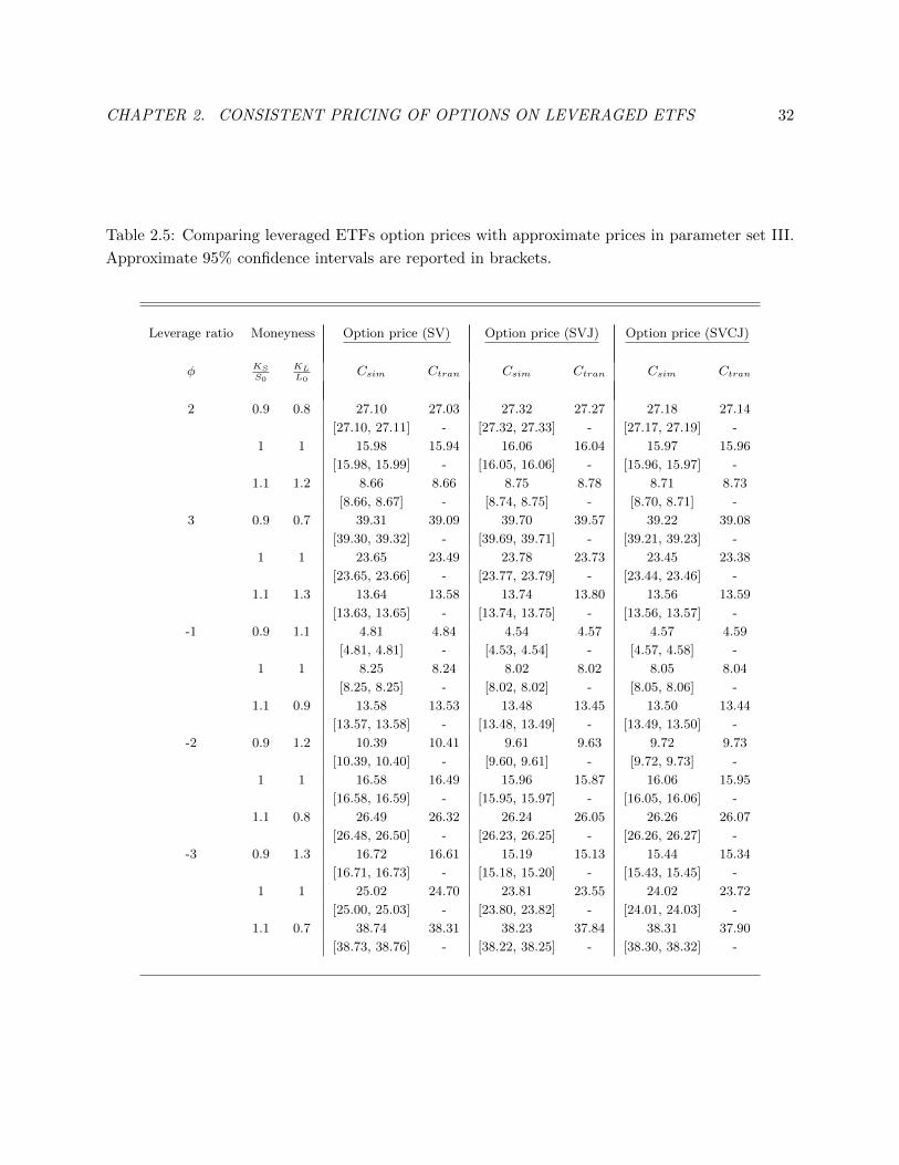
Table 2.5: Comparing leveraged ETFs option prices with approximate prices in parameter set III.

Approximate 95% confidence intervals are reported in brackets.


φ KSS0

KLL0


2 0.9 0.8 27.10 27.03 27.32 27.27 27.18 27.14

[27.10, 27.11] - [27.32, 27.33] - [27.17, 27.19] -

1 1 15.98 15.94 16.06 16.04 15.97 15.96

[15.98, 15.99] - [16.05, 16.06] - [15.96, 15.97] -

1.1 1.2 8.66 8.66 8.75 8.78 8.71 8.73

[8.66, 8.67] - [8.74, 8.75] - [8.70, 8.71] -

3 0.9 0.7 39.31 39.09 39.70 39.57 39.22 39.08

[39.30, 39.32] - [39.69, 39.71] - [39.21, 39.23] -

1 1 23.65 23.49 23.78 23.73 23.45 23.38

[23.65, 23.66] - [23.77, 23.79] - [23.44, 23.46] -

1.1 1.3 13.64 13.58 13.74 13.80 13.56 13.59

[13.63, 13.65] - [13.74, 13.75] - [13.56, 13.57] -

-1 0.9 1.1 4.81 4.84 4.54 4.57 4.57 4.59

[4.81, 4.81] - [4.53, 4.54] - [4.57, 4.58] -

1 1 8.25 8.24 8.02 8.02 8.05 8.04

[8.25, 8.25] - [8.02, 8.02] - [8.05, 8.06] -

1.1 0.9 13.58 13.53 13.48 13.45 13.50 13.44

[13.57, 13.58] - [13.48, 13.49] - [13.49, 13.50] -

-2 0.9 1.2 10.39 10.41 9.61 9.63 9.72 9.73

[10.39, 10.40] - [9.60, 9.61] - [9.72, 9.73] -

1 1 16.58 16.49 15.96 15.87 16.06 15.95

[16.58, 16.59] - [15.95, 15.97] - [16.05, 16.06] -

1.1 0.8 26.49 26.32 26.24 26.05 26.26 26.07

[26.48, 26.50] - [26.23, 26.25] - [26.26, 26.27] -

-3 0.9 1.3 16.72 16.61 15.19 15.13 15.44 15.34

[16.71, 16.73] - [15.18, 15.20] - [15.43, 15.45] -

1 1 25.02 24.70 23.81 23.55 24.02 23.72

[25.00, 25.03] - [23.80, 23.82] - [24.01, 24.03] -

1.1 0.7 38.74 38.31 38.23 37.84 38.31 37.90

[38.73, 38.76] - [38.22, 38.25] - [38.30, 38.32] -


re-balancing takes place continuously. We will see in Table 2.6 below that this is a principal

source of the discrepancy between the Monte-Carlo prices and the approximate prices.

(ii) Numerical transform inversion is also a source of error but we believe this error to be very

small and on the order of at most 1 or 2 cents. This claim is justified in part by the results

in Tables 2.2 and 2.3.

(iii) Statistical error in the reported Monte-Carlo prices. We ensured this error was small by

simulating sufficiently many paths so as to ensure that the approximate 95% confidence

intervals were just 1 or 2 cents wide.

(iv) The fourth source is of course the errors that arise from our approximations of the jump size

distributions in the SVJ and SVCJ models.

The main observation from Tables 2.4 and 2.5 is that the approximate LETF option prices as

reported in the Ctran columns are very close to the reported Monte-Carlo prices. In particular,

any discrepancy between the two should easily fall within the bid-ask spreads found in practice.

We also note that the Monte-Carlo prices are generally higher than the transform-based prices.

This is presumably due to the fact that prices computed via the transform approach are based

on continuous re-balancing of the LETFs whereas the Monte-Carlo prices are computed assuming

the LETF is re-balanced daily. We can confirm this observation by examining the option prices in

Table 2.6 where we also report Monte-Carlo prices that were estimated assuming the LETF was re-

balanced 4 times per day rather than just once per day. In that table we see that the Monte-Carlo

prices based on re-balancing four times per day are generally much closer to the transform based

prices. Presumably if we were to increase the LETF re-balancing frequency then the Monte-Carlo

and transform-based prices would be in even closer agreement. These observations justify our earlier


observation that most of the discrepancy in Tables 2.4 and 2.5 between the Monte-Carlo prices and

transform-based prices is due to the differences in re-balancing frequency rather than the quality of

our jump approximations. As stated above, however, this discrepancy in prices is sufficiently small

as to make little difference in practice. In contrast, we note that for the low-volatility environment

of parameter set I, the Monte-Carlo prices were generally lower (by just 1 or 2 cents) than the

transform prices. Again, if the LETF was re-balanced more frequently than daily re-balancing in

the Monte-Carlo then we would expect this difference to be even smaller.

Another observation from Tables 2.4 and 2.5 is that there is some discrepancy in LETF option

prices across the three different models. For example, in Table 2.4 we see that with φ = −3 and

KL/L0 = 1.75 the LETF call option price is approximately $51, $49 and $44 under the SV, SVJ

and SVCJ models, respectively. This is despite the fact that all three models were calibrated to the

same 6-month implied volatilities. Of course, this observation is not too surprising as the LETF

price is path-dependent and so it is not the case that the 6-month LETF option prices will only

depend on the risk-neutral distribution of St where t = 6 months. This difference in LETF option

prices across models is less noticeable in the 1-month options of parameter set III in Table 2.5. It

is also worth pointing out that the 6-month LETF option prices vary very little by model in the

low-volatility environment of parameter set I. These prices are displayed in Appendix A.4. We will

return to this issue in Section 2.7.3.

2.7.3 Comparing the LETF Implied Volatilities Across Different Models

We now report the LETF option prices of Section 2.7.2 in terms of their Black-Scholes implied

volatilities. We have already seen that there is some variability in these prices across the different

models but it would be interesting to see this variability expressed in units of implied volatility.


Table 2.6: Comparison of LETF option prices obtained by Monte-Carlo simulation with different

re-balancing frequencies in parameter set II. C(1)sim corresponds to daily re-balancing and C

(4)sim

corresponds to re-balancing 4 times per day. Ctran refers to prices that were obtained via numerical

transform inversion.


φ KSS0

KLL0

C(1)sim C

(4)sim Ctran C

(1)sim C

(4)sim Ctran C

(1)sim C

(4)sim Ctran

2 0.75 0.5 60.74 60.69 60.66 61.51 61.46 61.41 61.66 61.61 61.62

1 1 37.87 37.81 37.78 38.43 38.39 38.41 38.50 38.46 38.50

1.25 1.5 24.18 24.13 24.11 24.45 24.42 24.52 24.66 24.65 24.72

3 0.75 0.25 81.98 81.88 81.82 83.25 83.12 83.08 82.39 82.28 82.28

1 1 53.09 52.87 52.77 54.07 53.92 53.98 52.93 52.80 52.83

1.25 1.75 37.60 37.39 37.30 37.84 37.73 37.91 37.33 37.24 37.32

-1 0.75 1.25 14.15 14.14 14.14 13.93 13.90 13.87 12.63 12.62 12.59

1 1 21.19 21.16 21.15 21.16 21.12 21.03 20.00 19.97 19.91

1.25 0.75 32.79 32.74 32.73 33.24 33.18 33.01 32.25 32.21 32.11

-2 0.75 1.5 32.09 31.93 31.88 31.29 31.06 30.92 27.94 27.81 27.76

1 1 41.95 41.74 41.68 41.60 41.33 41.13 38.81 38.65 38.56

1.25 0.5 60.25 60.08 60.02 61.09 60.83 60.56 59.08 58.95 58.84

-3 0.75 1.75 51.48 50.80 50.72 49.43 48.59 48.47 44.41 43.99 43.86

1 1 60.88 60.24 60.17 59.56 58.72 58.57 55.77 55.36 55.21

1.25 0.25 81.74 81.43 81.46 82.59 81.96 81.82 80.65 80.48 80.39


This will also allow us to consider the commonly used practice of computing an LETF option

price via the Black-Scholes formula with the implied volatility taken (and scaled appropriately)

from a corresponding ETF option price. We will also introduce an additional model, namely the

Barndorff-Nielsen and Shephard (BNS) model (see [3]), as this model helps to provide an even

clearer demonstration of the fact that LETF option prices are strongly path dependent and are not

uniquely determined by the implied volatility surface of the underlying ETF. We first describe the

BNS model.

The BNS Model: The variance process is modeled by an Ornstein-Uhlenbeck process driven

by a Levy process with non-negative increments. In particular we will assume that the variance

process is a Gamma-OU process and that the risk-neutral dynamics for the security price and

instantaneous variance are

d logSt = (r − q −aλρ

b − ρ−Vt2)dt +

√VtdWt + ρdzλ⋅t

dVt = −λVtdt + dzλ⋅t

where Wt is a standard Brownian motion and zt is a compound Poisson process with zt = ∑Ntn=1 xn

where the Poisson process, Nt, has intensity, a, and the xi’s are IID exponential random variables

with mean 1/b. We also assume λ > 0 and V0 > 0 so that (since dzλ⋅t is always non-negative)

inf0≤t≤T Vt ≥ exp(−λT ) > 0. The parameter, ρ, is typically negative to account for the negative

correlation between variance and the underlying price process. Note that the variance can only

jump upwards and that between jumps it decays exponentially. With a negative value of ρ the

security price will jump downwards when a jump in variance occurs and it is worth noting in this

case that leveraged ETFs with φ < 0 can then only jump upwards in price. There is therefore no

need to truncate the jumps of the LETF price process in this case and indeed the LETF price


process will itself have BNS dynamics. When φ > 0 this will not be true as it will be necessary

to truncate the jumps of the underlying ETF. In this case we could try to approximate the jump-

process as we did with the SVJ and SVCJ models and then obtain approximate LETF option prices

using transform methods. Rather than doing this, however, we will simply price the LETF options

using Monte-Carlo because our goal in this section is to simply investigate how model dependent

LETF option prices are.

Table 2.7: Comparison for the prices of options on the leveraged ETFs obtained by Monte-Carlo

simulation in parameter sets II and III

Leverage ratio Moneyness Parameter Set II Moneyness Parameter Set III

φ KSS0

KLL0

CSVsim CSV Jsim CSV CJsim CBNSsimKSS0

KLL0

CSVsim CSV Jsim CSV CJsim CBNSsim

2 0.75 0.5 60.74 61.51 61.66 63.20 0.9 0.8 27.10 27.32 27.18 27.50

1 1 37.87 38.43 38.50 40.55 1 1 15.98 16.06 15.97 16.26

1.25 1.5 24.18 24.45 24.66 26.64 1.1 1.2 8.66 8.75 8.71 8.93

3 0.75 0.25 81.98 83.25 82.39 85.18 0.9 0.7 39.31 39.70 39.22 40.50

1 1 53.09 54.07 52.93 57.81 1 1 23.65 23.78 23.45 24.62

1.25 1.75 37.60 37.84 37.33 42.29 1.1 1.3 13.64 13.74 13.56 14.47

-1 0.75 1.25 14.15 13.93 12.63 11.53 0.9 1.1 4.81 4.54 4.57 4.39

1 1 21.19 21.16 20.00 18.92 1 1 8.25 8.02 8.05 7.86

1.25 0.75 32.79 33.24 33.25 31.48 1.1 0.9 13.58 13.48 13.50 13.35

-2 0.75 1.5 32.09 31.29 27.94 24.88 0.9 1.2 10.39 9.61 9.72 9.18

1 1 41.95 41.60 38.81 36.15 1 1 16.58 15.96 16.06 15.50

1.25 0.5 60.25 61.09 59.08 57.72 1.1 0.8 26.49 26.24 26.26 25.88

-3 0.75 1.75 51.48 49.43 44.41 39.00 0.9 1.3 16.72 15.19 15.44 14.36

1 1 60.88 59.56 55.77 51.48 1 1 25.02 23.81 24.02 22.97

1.25 0.25 81.74 82.59 80.65 79.48 1.1 0.7 38.74 38.23 38.31 37.64

We calibrated the BNS model to the same implied volatility skews of Figure 2.2 and note here

that this calibration was performed successfully so that all four models agreed on the prices of

options on the underlying ETF. This agreement can be seen in Tables 2.8 and 2.9 by noting that

the columns labeled ΣS are practically identical across the four models. The prices of the LETF

options across the four models and various leverage ratios are displayed in Table 2.7. The same


results, except in terms of implied volatilities, are displayed in Tables 2.8 and 2.9 for parameter sets

II and III, respectively. The LETF option implied volatilities are displayed in the columns labeled

ΣL and are calculated using the LETF option prices from Tables 2.4 and 2.5.

In order to compute the implied volatility ratios, ΣLΣS

, we aligned the options on the underlying

ETF and the leveraged ETF on a “strike-equivalent-basis” to account for the leverage. For example,

we align a 25% OTM option on the underlying ETF with a 50% OTM option on a double-long

LETF to account for the higher leverage of φ = 2. We note that the implied volatility ratio tends

to be close to the leverage ratio, φ, but that there can be a considerable discrepancy between the

two. The degree of this discrepancy is model dependent and is very notable for the BNS model

(which is why we have included the BNS model here). For a given model, it is also the case that

whether or not the ratio ΣLΣS

is greater than φ depends on whether or not the LETF is positively

or negatively leveraged. We emphasize again here that these observations are based on parameter

set II which models the 6-month, high volatility environment.

2.8 Conclusions

We have shown how to obtain accurate LETF option prices via transform pricing methods for the

Heston model as well as two related jump-diffusion models. Our approximations work well in both

low and high volatility environments and because they are consistent with the prices of options on

the underlying ETF, they permit consistent pricing and risk-management of derivatives portfolios

containing both ETF and LETF options. It should also be clear that similar approximation tech-

niques could be applied to other jump-diffusion models and so our examples should be viewed as

applications of a more general approximation technique.


In addition to confirming the accuracy of our LETF option prices, our numerical experiments

also showed that the ratio of an LETF option implied volatility to the corresponding ETF option

implied volatility can be far from the LETF leverage ratio. The difference between the two depends

on whether or not the LETF is long or short and is model dependent, thereby emphasizing the path

dependence of the LETF price at any given time. This calls into question the market practice of

pricing an LETF option using the Black-Scholes formula with the strike and implied volatility from

the underlying ETF scaled by the leverage ratio. In particular, it should be clear that using the

Black-Scholes formula in this manner amounts to the implicit assumption of (generally unspecified)

dynamics for the underlying ETF.


Tab

le2.8

:C

om

pari

son

ofB

lack

-Sch

oles

Imp

lied

-Vol

atil

itie

s:P

aram

eter

Set

II

Lev

erage

rati

oM

oney

nes

sIm

plied

Vola

tility

(SV

)Im

plied

Vola

tility

(SV

J)

Implied

Vola

tility

(SV

CJ)

Implied

Vola

tility

(BN

S)

φK

SS0

KL

L0

ΣS

ΣL

ΣL

ΣS

ΣS

ΣL

ΣL

ΣS

ΣS

ΣL

ΣL

ΣS

ΣS

ΣL

ΣL

ΣS

20.7

50.5

75.4

2149.1

01.9

875.4

4154.6

12.0

575.4

0155.7

32.0

775.4

1166.6

82.2

1

11

71.2

8139.1

11.9

571.1

0141.3

51.9

971.1

3141.6

21.9

971.0

9149.9

82.1

1

1.2

51.5

68.0

0133.1

21.9

667.9

8134.0

71.9

768.0

5134.8

51.9

868.0

4141.8

82.0

9

30.7

50.2

5224.1

82.9

7242.3

13.2

1230.0

53.0

5270.1

43.5

8

11

204.2

02.8

6208.7

62.9

4203.5

02.8

6226.6

63.1

9

1.2

51.7

5195.8

82.8

8196.7

62.8

9194.8

92.8

6213.5

23.1

4

-10.7

51.2

578.4

81.0

477.6

91.0

373.0

40.9

769.0

70.9

2

11

75.2

91.0

675.2

01.0

670.9

31.0

066.9

50.9

4

1.2

50.7

571.1

11.0

573.3

61.0

868.3

91.0

164.4

40.9

5

-20.7

51.5

161.4

72.1

4158.5

52.1

0146.5

21.9

4135.6

21.8

0

11

155.7

02.1

8154.2

62.1

7142.9

02.0

1132.2

31.8

6

1.2

50.5

145.6

02.1

4151.6

02.2

3137.0

82.0

1126.9

91.8

7

-30.7

51.7

5250.1

13.3

2241.6

73.2

0221.6

72.9

4201.0

72.6

7

11

242.0

43.4

0235.3

43.3

1216.7

93.0

5196.8

62.7

7

1.2

50.2

5220.8

23.2

5232.9

53.4

3205.0

73.0

1187.5

62.7

6


Tab

le2.

9:

Com

par

ison

ofB

lack

-Sch

oles

Imp

lied

-Vol

atil

itie

s:P

aram

eter

Set

III

Lev

erage

rati

oM

oney

nes

sIm

plied

Vola

tility

(SV

)Im

plied

Vola

tility

(SV

J)

Implied

Vola

tility

(SV

CJ)

Implied

Vola

tility

(BN

S)

φK

SS0

KL

L0

ΣS

ΣL

ΣL

ΣS

ΣS

ΣL

ΣL

ΣS

ΣS

ΣL

ΣL

ΣS

ΣS

ΣL

ΣL

ΣS

20.9

0.8

74.7

0149.2

92.0

074.4

3151.8

62.0

474.3

3150.1

92.0

274.4

7153.9

22.0

7

11

71.5

9142.2

81.9

971.0

9142.9

82.0

171.1

0142.1

82.0

071.0

9144.8

22.0

4

1.1

1.2

68.6

8136.3

71.9

968.5

5137.1

32.0

068.6

1136.7

81.9

968.5

7138.8

22.0

2

30.9

0.7

224.4

23.0

0229.5

03.0

8223.2

23.0

0239.8

93.2

2

11

212.5

12.9

7213.6

53.0

1210.6

22.9

6221.4

53.1

2

1.1

1.3

203.5

02.9

6204.4

22.9

8202.8

22.9

6210.9

23.0

8

-10.9

1.1

75.3

81.0

172.7

80.9

873.1

40.9

871.4

10.9

6

11

72.9

01.0

270.8

51.0

071.1

61.0

069.4

00.9

8

1.1

0.9

70.0

61.0

269.0

41.0

169.1

81.0

167.5

50.9

9

-20.9

1.2

152.1

42.0

4145.0

41.9

5146.0

81.9

7141.1

01.8

9

11

147.7

32.0

6142.0

92.0

0142.9

52.0

1137.9

41.9

4

1.1

0.8

142.1

32.0

7139.1

22.0

3139.4

32.0

3134.8

01.9

7

-30.9

1.3

231.0

03.0

9217.3

92.9

2219.5

72.9

5209.9

32.8

2

11

225.1

73.1

5213.9

53.0

1215.8

93.0

4206.2

12.9

0

1.1

0.7

216.9

63.1

6210.2

43.0

7211.2

53.0

8202.3

12.9

5

CHAPTER 3. LINEAR PROGRAMMING AND THE CONTROL OF DIFFUSIONPROCESSES 42

Chapter 3

Linear Programming and the Control

of Diffusion Processes

3.1 Introduction

Due to the so-called curse-of-dimensionality, solving high dimensional control problems is a no-

toriously difficult problem. It is not surprising then that sub-optimal control has been an active

area of research for many years. Moreover, the advent of ever-increasing computational power

has seen many developments1 in the related area of approximate dynamic programming (ADP),

particularly for discrete-time control problems. Linear programming (LP) methods have played

an important role in the development of several ADP techniques, beginning with Schweitzer and

Seidmann [34] and continuing with the important contributions of de Farias and Van Roy [12;

13] among others.

1 See Bertsekas [6] for a comprehensive introduction to classical sub-optimal control techniques. Bertsekas [7]

also contains an excellent treatment of approximate dynamic programming.


Recently, Han and Van Roy [19] proposed an LP-based approach for the approximate solution

of the HJB equation that arises from continuous-time control problems. Their approach applies to

diffusion problems with an exponentially-distributed horizon, T , and their numerical results were

promising, with the LP-based policy outperforming other base-case policies. In this chapter we

extend their approach to continuous-time control problems with a fixed horizon, T . We apply these

techniques to dynamic portfolio optimization problems and then simulate the resulting policies

to obtain primal, i.e. lower, bounds on the optimal value functions. We also use these policies

in conjunction with the convex duality methodology2 of Haugh, Kogan and Wang [22] (hereafter

HKW) to construct dual, i.e. upper, bounds on the optimal value functions. By comparing the

resulting primal and dual bounds we can easily assess the quality of the sub-optimal policy produced

by the LP-approach. In our numerical experiments we find that the primal and dual bounds are

very close and so we can conclude that, for these problems at least, the LP approach performs very

well indeed.

The remainder of this chapter is organized as follows. In Section 3.2 we formulate the continuous-

time portfolio optimization problem and also discuss here the exponentially distributed and fixed

horizon versions of the problem. In Section 3.3 we review the approach of Han and Van Roy for

approximately solving the HJB equation when the horizon is an exponentially distributed random

variable. We extend their methodology to the fixed horizon case in Section 3.4 and our numerical

results are presented in Section 3.5. We conclude in Section 3.6. The appendices contain additional

details including an overview of the aforementioned dual approach of HKW.

2See also Haugh and Jain [21].


3.2 The Portfolio Optimization Problem Formulation

We formulate the dynamic portfolio3 optimization problems that we will consider throughout the

chapter. We will follow the formulation of HKW. There are N risky stocks and an instantaneously

risk-free bond in a market. The vector of stock prices is denoted by Pt = (P1t,⋯, PNt)⊺ and the

instantaneously risk-free rate of return on the bond is denoted by rt. Without loss of generality, we

assume the stocks pay no dividends. Assets return dynamics depend on the M -dimensional vector

of state variables, Zt = (Z1t,⋯, ZMt)⊺, so that

rt = r(Zt), (3.1a)

dPtPt

= µP (Zt)dt +ΣP (Zt)dBt, (3.1b)

dZt = µZ(Zt)dt +ΣZ(Zt)dBt (3.1c)

where Bt = (B1t,⋯,BNt)⊺ is an N -dimensional standard Brownian motion. µZ(Zt) and µP (Zt) are

M - and N -dimensional drift vectors, while ΣZ(Zt),ΣP (Zt) are M ×N and N ×N diffusion matrices

of the state variable and security prices, respectively. We assume the diffusion matrix, ΣP (Zt), of

the asset return process is non-degenerate for each Zt so that x⊺ΣP (Zt)ΣP (Zt)⊺x ≥ ε∣∣x∣∣2 for all x

and some ε > 0. We can then define a process, ηt, according to

ηt(Zt) ∶= ΣP (Zt)−1

(µP (Zt) − r(Zt) ⋅ 1)

where 1 = (1,⋯,1)⊺. In a market without portfolio constraints, ηt corresponds to the market-price-

of-risk process (e.g. Duffie 1996 [14], Section 6.G). We make the standard assumption that the

3 We do note here, however, that the LP-based approach to solving the HJB equation applies to control problems

in diffusion settings more generally.


process ηt is square integrable so that4

E0[∫

T

0∥ ηt ∥

2 dt] <∞.

Under this opportunity set, our portfolio consists of positions in the N stocks and the risk-free

bond. We also assume that continuous re-balancing of the portfolio is permitted and that θt(Zt) ∶=

(θ1t(Zt),⋯, θNt(Zt))⊺ is the vector of risky security weights in the portfolio at time t. To rule out

arbitrage, we require the portfolio strategy to satisfy a square integrability condition, namely that

∫T

0 ∣∣θ∣∣2dt < ∞. The value of the portfolio, Wt, associated with θt then changes according to the

SDE:

dWt

Wt= [rt + θ

⊺t λt]dt + θ

⊺t ΣPtdBt (3.2)

where λt ∶= µPt − rt ⋅ 1.5 We also assume that the portfolio is constrained so that

θt(Zt) ∈ K, (3.3)

for all t and where K is some fixed convex set containing zero.

The portfolio optimization problem is to choose a self-financing trading strategy that maximizes

the expected utility of terminal wealth. The horizon, T , is assumed to be finite but it may be either

random or deterministic, depending on the specific formulation under consideration. The utility

function u(W ) is assumed to be strictly increasing, concave and smooth. Moreover, it is assumed to

satisfy the Inada conditions at zero and infinity so that limW→0 u′(W ) =∞ and limW→∞ u

′(W ) = 0.

In this chapter, we will use the constant relative risk aversion (CRRA) utility function so that

u(W ) ∶=W 1−γ

1 − γ

4 We use Et[⋅] to denote an expectation conditional on time t information throughout the chapter.

5 We use r, µP , µZ ,ΣP ,ΣZ , η, θ, λ (or rt, µPt , µZt ,ΣPt ,ΣZt , ηt, θt, λt) instead of r(Zt), µP (Zt), µZ(Zt),ΣP (Zt),ΣZ(Zt), ηt(Zt), θt(Zt), λ(Zt) for simplicity, if their meanings are clear.


with γ ≥ 1.

3.2.1 When the Horizon, T , is Fixed

When the problem has a fixed horizon, T , the investor’s portfolio optimization problem at time t

is to solve for

J∗(w, z, t) = sup{θs}

Et [u(WT )] subject to (1), (2) and (3) (3.4)

where w and z are the wealth and state vector values at time t. A well-known implication of CRRA

utility is that J∗ is separable in w and (z, t) so that we can write J∗(w, z, t) = u(w)V ∗(z, t). The

optimal strategy is therefore independent of the wealth process, wt.

In order to write the HJB equation for this problem we first define the HJB operator

HθV (z, t) ∶= (1 − γ)V (z, t)(θ⊺λ + r) + Vz(z, t)⊺µZ(z) +

1

2γ(γ − 1)V (z, t)θ⊺ΣPΣ⊺

P θ (3.5)

+(1 − γ)Vz(z, t)⊺ΣZΣ⊺

P θ +1

2tr[Vzz(z, t)ΣZΣ⊺

Z] + Vt(z, t).

Note that Vz is the M -dimensional gradient of V with respect to the state variable z. Similarly Vzz

is the M ×M Hessian matrix of V with respect to z. The HJB equation is then given by

0 =HV (z, t) ∶= infθ∈K

HθV (z, t) (3.6)

and we note that V ∗(z, t) = J∗(w, z, t)/u(w) is a solution to this equation.

3.2.2 When the Horizon, T , is Exponentially Distributed

When the horizon T is an exponentially distributed random variable with mean τ , the investor’s

problem is identical to (3.4) but now with the understanding that the expectation must also be

taken with respect to T . By first taking expectation with respect to T it is easy to see the problem


may also be formulated as

J∗(w, z) = sup{θs}

E [∫

∞

t=0e−t/τu(Wt)dt] subject to (1), (2) and (3). (3.7)

While t is no longer a state variable, J∗ is still separable so we can again write J∗(w, z) =

u(w)V ∗(z). The HJB operator for this problem is then defined as

HθV (z) ∶= (1 − γ)V (z)(θ⊺λ + r) + Vz(z)⊺µZ(z) +

1

2γ(γ − 1)V (z)θ⊺ΣPΣ⊺

P θ (3.8)

+(1 − γ)Vz(z)⊺ΣZΣ⊺

P θ +1

2tr[Vzz(z)ΣZΣ⊺

Z] −V (z)

τ+ 1.

and the HJB equation is given by

0 =HV (z) = infθ∈K

HθV (z). (3.9)

We note that V ∗(z) = J∗(w, z)/u(w) is a solution to this equation.

3.3 Review of Han and Van Roy’s LP Approach

In this section we review Han and Van Roy’s[19] LP approach for approximately solving (3.7) when

the horizon T is exponentially distributed. In a standard argument they show the optimal solution,

V ∗, to the HJB equation (3.9) is also the unique optimum of the following static optimization

problem:

maxV (z)

∫ V (z)ρ(dz)

subject to HθV (z) ≥ 0, ∀ θ, z (P1)

V ∈ C2

where ρ is a pre-specified positive measure for the integral. While the objective and constraints in

(P1) are linear the problem is still very challenging to solve as there are uncountably many decision


variables and constraints; indeed there is one constraint for every (θ, z) pair. We therefore solve

an approximation to (P1) and this approximation is obtained via the following steps:

1. We first choose a suitable set of basis functions {φ1(z),⋯, φk(z)} with the goal of finding

a linear combination, ∑kj=1 rjφj(z), that we will use to approximate V ∗(z). The original

problem then reduces to the problem of solving for k decision variables, r1, r2,⋯, rk. The

algorithm is initialized with a predetermined weight vector, r(0) = (r(0)1 ,⋯, r

(0)k ).

2. We generate a finite sample set z1, . . . , zQ and approximate the integral in (P1) by a corre-

sponding finite sum of Q terms. While any positive measure, ρ, can be used in theory, the

performance of the algorithm depends on how the samples are generated. Han and Van Roy

define

ρ(dz) ∶=1

τE[∫

∞

t=0e−t/τ1{Zt∈[z,z+dz]}dt]

and then generate z1, . . . , zQ by simulating (approximately) from this measure. In particular,

they first simulate the horizon T ∼ Exp(1/τ) and then simulate a discrete-time approximation

to the dynamics of the state variables (3.1c). The value of the state vector at the simulated

time T is taken as one of our Q samples.

3. For each sample, zj , we choose a single corresponding θj as follows: given an approximation,

Φr ∶= φ1r1 +⋯+ φkrk, to V ∗, we myopically choose a greedy action with respect to Φr. That

is, we select θj ∈ argminθ∈K

Hθ [(Φr) (zj)] for each j.

4. Given a weight vector r, we find a new weight vector r′ by solving an approximation of (P1)

(see phase 2 of the algorithm below); this approximation is a linear program that we obtain

from steps 1 to 3.


Steps 3 and 4 are repeated to obtain a sequence of weight vectors, {r(0), r(1), r(2),⋯}. We are

now ready to define the adaptive constraint selection algorithm of Han and Van Roy:

Adaptive Constraint Selection Algorithm I

for i = 1 to ∞ do

for j = 1 to Q do

θj ∈ argminθ∈K

Hθ [(Φr(i−1)

)(zj)] (phase 1)

end for

r(i) ∈ argmaxr∈Rk

Q

∑j=1

(Φr)(zj) (phase 2)

subject to Hθj [(Φr)(zj)] ≥ 0, ∀j = 1,⋯,Q

end for

This algorithm does not necessarily generate an optimal solution to (P1) and there is no6

theoretical guarantee that the sequence r(i) will converge. However, if it does converge then Han

and Van Roy[19] show it must converge to an optimal solution of the following problem which is

an approximation of (P1):

maxr

Q

∑j=1

(Φr)(zj)

subject to H [(Φr)(zj)] ≥ 0, ∀j = 1,⋯,Q. (3.10)

We now discuss in further detail the steps required to execute phases 1 and 2.

6 Han and Van Roy did not specify how they handled non convergence. We suspect they simply used a different

starting point, r(0), if that occurred.


Phase 1

We can expand the objective of phase 1 using (3.8). If we then remove terms that do not depend

on θ and eliminate the common factor, (γ − 1), then the problem of phase 1 can be expressed as:


1

2θ⊺[γ(Φr(i−1)

)(zj)ΣPΣ⊺P ]θ − [(Φr(i−1)

)(zj)λ(zj) +ΣPΣ⊺Z(Φr

(i−1))z(zj)]

⊺

θ. (3.11)

If (Φr(i−1))(zj) > 0, then (3.11) is a convex quadratic program and therefore easy to solve. Oth-

erwise the objective in (3.11) may be unbounded if K is not compact and some other heuristic

approach for computing θj would be required.

Phase 2

If we expand the constraints of the LP in phase 2 using (3.8), then we obtain the following LP:

maxr∈Rk

c⊺r

subject to Ar ≥ −1 (3.12)

where

Aij ∶=(1 − γ)φj(zi)[θ⊺i λ(zi) + r(zi)] + [(φj)z(zi)]

⊺µZ(zi) +

1

2γ(γ − 1)φj(zi)θ

⊺i ΣPΣ⊺

P θi

+ (1 − γ)[(φj)z(zi)]⊺

ΣZΣ⊺P θi +

1

2tr[(φj)zz(zi)ΣZΣ⊺

Z] −φj(zi)

τ

and ci ∶= φi(z1)+ φi(z2)+⋯+φi(zQ). This linear program has a k-dimensional decision vector and

Q linear constraints.


3.4 Extending the LP Approach to the Case of a Fixed Horizon,

T

The LP approach of the previous section applies to problems with an exponentially distributed

horizon, T , but we would also like to apply it to the case of a fixed horizon. As we shall see,

this extension is not immediate and requires some work due to the fact that time t is also a state

variable in this case. We show in Appendix B.1 that under some technical conditions, that the

solution to the HJB equation (3.6), V ∗, is also the unique optimum to the following optimization

problem:

maxV

∫ V (z, t)ρ(dz, dt)

subject to HθV (z, t) ≥ 0, ∀ θ, z, t (P2)

V (z, T ) ≤ 1, ∀ z (boundary condition)

V ∈ C2

where ρ is again some pre-specified measure. In contrast to problem (P1), the boundary condition

V (z, T ) ≤ 1 is required in this case.

The extension of the adaptive constraint selection algorithm seems straightforward: we choose

basis functions {φ1(z, t),⋯, φk(z, t)} to approximate V ∗(z, t) and generate {(z1, t1), (z2, t2),⋯, (zQ, tQ)}

as a representative sample of (z, t). As a simple heuristic for generating this sample, we first gen-

erate the tj ’s as IID ∼ U[0, T ] and then, for each tj , we set zj ∶= Ztj where Ztj is obtained by

simulating a discrete-time approximation to the market state dynamics (3.1c) and then terminat-

ing at time tj . The adaptive constraint selection algorithm in this case is as follows:


Adaptive Constraint Selection Algorithm II (For a Fixed Horizon T )

for i = 1 to ∞ do

for j = 1 to Q do


Hθ [(Φr(i−1)

)(zj , tj)] (phase 1)

end for


Q

∑j=1

(Φr)(zj , tj) (phase 2)

subject to Hθj [(Φr)(zj , tj)] ≥ 0, ∀ j = 1,⋯,Q,

(Φr)(z, T ) ≤ 1, ∀ z

end for

We note the boundary condition (Φr)(z, T ) ≤ 1 in phase 2 applies to all possible z rather than

just the sampled zj ’s. We could of course impose this boundary constraint on just a finite subset of

z values but we will see later that it is straightforward to impose the general constraint through an

appropriate choice of basis functions. For example, we could ensure that each non-constant basis

function has a common factor (T − t). As a result, the only contribution to the left-hand side of

the constraint (Φr)(z, T ) ≤ 1 will come from a constant basis function, say φ1 ≡ 1. We can then

impose the boundary condition by adding the linear constraint r1 ≤ 1 to the LP phase 2.

We now discuss the objectives and constraints in phases 1 and 2 in further detail and in par-

ticular, why this algorithm is problematic to implement in its current form.


Phase 1

If we substitute (3.5) into the objective function of phase 1, drop all terms that do not depend on

θ and eliminate the common factor, (γ − 1), then the problem of phase 1 may be written as:


1

2θ⊺[γ(Φr(i−1)

)(zj , tj)ΣPΣ⊺P ]θ (3.13)

−[(Φr(i−1))(zj , tj)λ(zj) +ΣPΣ⊺

Z(Φr(i−1)

)z(zj , tj)]⊺

θ.

If (Φr(i−1))(zj , tj) > 0, then the phase 1 problem is a convex quadratic program and therefore easy

to solve. Otherwise, depending on K, (3.13) may be unbounded. In this case we simply take θj to

be the myopic portfolio which is described in Appendix B.2. We note here, however, that in our

numerical experiments it only rarely7 occurred that (Φr(i−1))(zj , tj) < 0.

Phase 2

If we substitute (3.5) into the constraints of phase 2, then the problem of phase 2 can be formulated

as:

maxr∈Rk

c⊺r

subject to Ar ≥ 0 (3.14)

(Φr)(z, T ) ≤ 1, ∀z

where

Aij =(1 − γ)φj(zi, ti)[θ⊺

i λ(zi) + r(zi)] + (φj)z(zi, ti)⊺µZ(zi) +

1

2γ(γ − 1)φj(zi, ti)θ

⊺

i ΣP Σ⊺P θi

+ (1 − γ)[(φj)z(zi, ti)]⊺

ΣZΣ⊺P θi +1

2tr[(φj)zz(zi, ti)ΣZΣ⊺Z] + (φj)t(zi, ti),

7 In the numerical experiments of Section 3.5.1, we considered problems with various combinations of risk-aversion

parameter, γ, and horizon T . In the worst-case among all such problems, we observed (Φr(i−1))(zj , tj) < 0 only 1.46%

of the time. In most of these problems (Φr(i−1))(zj , tj) < 0 never actually occurred.


ci = φi(z1, t1) + φi(z2, t2) + ⋯ + φi(zQ, tQ). Ignoring the boundary conditions, (Φr) (⋅, T ) ≤ 1, (which

we can handle through the choice of basis functions as previously discussed), we see that phase 2

is an LP with a k-dimensional decision vector and Q linear constraints.

It turns out that phase 2 here is very problematic. In particular, the constraint Ar ≥ 0 of

(3.14) is much more difficult to handle than the constraint Ar ≥ −1 of (3.12) which occurs in

the exponentially distributed horizon case. This latter set of constraints is always satisfied by all

points in some ball around the zero vector 0. This is not true in the fixed horizon case where

the corresponding constraints are Ar ≥ 0. Since r is k-dimensional, each of the Q constraints in

Ar ≥ 0 defines a k-dimensional closed half-space containing 0 on its boundary. Any feasible point

must therefore lie in the intersection of these Q half-spaces. Moreover, since Q is typically much

larger than k the intersection is generally just a single-point, namely the origin {0}. This makes

the problem (3.14) trivial to solve but the solution is hardly desirable.

One ad-hoc approach for resolving this issue would be to relax the constraint Ar ≥ 0 to Ar ≥ −ε⋅1

where ε is some small positive number. For example, in our initial numerical experiment of Section

3.5.1, the value ε = 1 appeared to yield the best results among several different values of ε. We did

not, however, have a sensible rule for choosing an appropriate value of ε in advance. Moreover, in

Section 3.4.1 below we propose an alternative problem formulation that yields superior results.

3.4.1 An Alternative Formulation

We propose here a new problem formulation that is based on the certainty equivalent return,

rce, which is defined as the certain annualized rate of return which makes the investor indifferent

between accepting it and following his optimal trading strategy. It is therefore given implicitly via

u(w)V ∗(z, t) = u (werce(z,t)(T−t)) ,


which implies

ln (V ∗(z, t)) = rce(z, t)(T − t)(1 − γ). (3.15)

Because rce(z, t) is generally “less non-linear” than the value function (especially when γ is large),

it makes some sense to approximate the log-value function rather than the value function itself.

We assume basis functions of the form

{φ1(z, t),⋯, φk(z, t)} = {(T − t)φ1(z, t),⋯, (T − t)φk(z, t)} (3.16)

and will use a linear combination of them to approximate ln (V ∗(z, t)). We also note that any such

linear combination of these functions will automatically satisfy the boundary condition e(Φr)(z,T ) ≤ 1

so that this constraint does not need to be explicitly imposed in our new adaptive constraint selec-

tion algorithm:


Adaptive Constraint Selection Algorithm III (For a Fixed Horizon T )

for i = 1 to ∞ do

for j = 1 to Q do


Hθ [e(Φr(i−1))(zj ,tj)] (phase 1)

end for


Q

∑j=1

e(Φr)(zj ,tj) (phase 2)

subject to Hθj [e(Φr)(zj ,tj)] ≥ 0, ∀ j = 1,⋯,Q

end for

We provide further details on the steps required for phases 1 and 2 below.

Phase 1

If we substitute (3.5) into the objective function of phase 1, drop terms that do not depend on θ

and then eliminate the common factor, eΦr(i−1)(γ −1), then the problem of phase 1 may be reduced

to:


1

2θ⊺[γΣPΣ⊺

P ]θ − [λ (zj) +ΣPΣ⊺Z (Φr(i−1)

)z(zj , tj)]

⊺

θ (3.17)

where the subscript z in (3.17) denotes a gradient vector. In contrast to the previous algorithm,

phase 1 is always a convex quadratic program and therefore easy to solve.


Phase 2

Similarly, if we substitute (3.5) into the constraints of phase 2, eliminate the common factor eΦr

and rearrange, we obtain:8

(Φr)z(z, t)⊺µZ(z) + (1 − γ)(Φr)z(z, t)

⊺ΣZΣ⊺P θ +1

2tr[((Φr)zz(z, t) + (Φr)z(z, t)(Φr)z(z, t)

⊺)ΣZΣ⊺Z]

+ (Φr)t(z, t) ≥ − (1 − γ)(θ⊺λ + r) −1

2γ(γ − 1)θ⊺ΣP Σ⊺P θ. (3.18)

for (z, t) = (z1, t1), . . . , (zQ, tQ). Note the phase 2 objective function contains the exponential term

e(Φr)(zj ,tj) and the constraint (3.18) contains the term (Φr)z(z, t)(Φr)z(z, t)⊺ which is quadratic

in r. Phase 2 is therefore not an LP.

We resolve this problem by: (i) linearizing the objective function using a first-order Taylor series

expansion of ex around zero and (ii) simply dropping9 the terms in (3.18) that quadratic in r. This

yields the following LP for phase 2

maxr∈Rk

c⊺r

subject to Ar ≥ −d (3.19)

where

Aij ∶= (φj)z (zi, ti)⊺

µZ (zi) + (1 − γ) [(φj)z (zi, ti)]⊺

ΣZΣ⊺P θi+

1

2tr [(φj)zz (zi, ti)ΣZΣ⊺Z] + (φj)t (zi, ti) ,

di ∶= (1 − γ) [θ⊺i λ (zi) + r (zi)] +1

2γ(γ − 1)θ⊺i ΣP Σ⊺P θi,

ci ∶= φi (z1, t1) + φi (z2, t2) +⋯ + φi (zQ, tQ) .

8 Note that if we used the alternative formulation based on approximating the log-value function for the case of

the exponentially distributed horizon, we would not be able to eliminate the factor eΦr due to the constant term “1”

that appears in the HJB operator in (3.8).

9 We could of course also have used a Taylor expansion to linearize the constraints but in our numerical experiments

we obtained very good results by simply dropping the quadratic terms.


In our numerical experiments with this algorithm we will choose φ1(z, t) =T−tT as one of our basis

function. It is then easy to see that A1j =T−tjT > 0 for all j so regardless of d, we can ensure Ar ≥ −d

holds by taking r1 sufficiently large. We therefore do not need to relax the constraints, Ar ≥ −d,

as we needed to do with (3.14) in our original problem formulation for the problem with a fixed

horizon, T .

3.5 Numerical Experiments

We now illustrate the performance of the LP-based algorithms of Section 3.4. We consider several

portfolio optimization problems and assume that in each of them the horizon, T , is fixed. We

consider three different trading strategies: the strategies that are greedy with respect to the ap-

proximate value functions that are obtained from the adaptive constraint selection algorithms II

and III, respectively, as well as the well-known myopic strategy10 which we will use as a benchmark.

The LB-based strategies at any state (t,Zt) are found by solving

θLP1t = argmin

θ∈K

1

2θ⊺[γ (Φr∗) (Zt, t)ΣPΣ⊺

P ]θ (3.20)

−[(Φr∗) (Zt, t)λ +ΣPΣ⊺Z (Φr∗)z (Zt, t)]

⊺

θ,

θLP2t = argmin

θ∈K

1

2θ⊺[γΣPΣ⊺

P ]θ − [λ +ΣPΣ⊺Z (Φr∗)z (Zt, t)]

⊺

θ. (3.21)

We note that θLP1t and θLP2

t are obtained from (3.13) and (3.17), i.e. phase 1 of Algorithms II and

III, respectively, by replacing Φr with Φr∗, where r∗ is the solution we obtain from implementing

these algorithms. Similarly the myopic strategy in state (t,Zt) is found by solving the convex

10 The myopic strategy is known to perform well under the various numerical experiments in HKW [22] and Haugh

and Jain [21]. Indeed when γ = 1 it is known to be the optimal strategy. Further details on the myopic strategy can

be found in Appendix B.2.


quadratic program

θmt = argminθ∈K

1

2θ⊺ [γΣPΣ⊺

P ] θ − λ⊺θ (3.22)

where λ is the time t vector of excess returns.

We use a simple Euler scheme to generate sample paths of the security prices and state vector,

Zt. At each time step all three strategies are found by solving (3.20), (3.21) and (3.22), respectively.

By simulating many paths and averaging the utility of terminal wealth across all paths for each

strategy we can obtain estimates of the value functions associated with each of the strategies. In

our numerical results we will report these value functions as certainly equivalent (CE) annualized

returns. Since these strategies are all feasible their CE returns are therefore lower bounds on the

CE return for the (in general) unknown optimal strategy. Finally we can use the dual approach of

HKW11 to construct upper bounds on the optimal value. These upper bounds are also reported as

CE returns.

3.5.1 Example I

Our first numerical example is from HKW who in turn based their model on the discrete-time

market model in Lynch [29]. They consider a financial market with three risky assets and a single

state variable associated with a four-dimensional Brownian motion. In our framework of Section

3.2 we assumed (without loss of generality) that the volatility matrix, ΣP , is invertible. We can

enforce this here by simply assuming that the state variable is in fact a fourth risky security that

we are not allowed to trade. We assume the drift term of risky assets returns is affine in the state

variable which itself follows an Ornstein-Uhlenbeck process with a long-term mean of zero. The

11See Appendix B.3 for a review of their dual methodology.


asset return dynamics therefore satisfy:

rt ≡ r,

dPtPt

= (µ0 +Ztµ1)dt +ΣPdBt,

dZt = −kZtdt +ΣZdBt

where r = .01, k = 0.366 and

µ0 =

⎡⎢⎢⎢⎢⎢⎢⎢⎢⎢⎢⎢⎢⎣

0.142

0.109

0.089

⎤⎥⎥⎥⎥⎥⎥⎥⎥⎥⎥⎥⎥⎦

, µ1 =

⎡⎢⎢⎢⎢⎢⎢⎢⎢⎢⎢⎢⎢⎣

0.065

0.049

0.049

⎤⎥⎥⎥⎥⎥⎥⎥⎥⎥⎥⎥⎥⎦

, ΣP =

⎡⎢⎢⎢⎢⎢⎢⎢⎢⎢⎢⎢⎢⎢⎢⎢⎢⎢⎣

0.256 0 0 0

0.217 0.054 0 0

0.207 0.062 0.062 0

−0.741 0.04 0.034 0.288

⎤⎥⎥⎥⎥⎥⎥⎥⎥⎥⎥⎥⎥⎥⎥⎥⎥⎥⎦

, ΣZ =

⎡⎢⎢⎢⎢⎢⎢⎢⎢⎢⎢⎢⎢⎢⎢⎢⎢⎢⎣

−0.741

0.04

0.034

0.288

⎤⎥⎥⎥⎥⎥⎥⎥⎥⎥⎥⎥⎥⎥⎥⎥⎥⎥⎦

⊺

.

Note that r,ΣP and ΣZ are constant in this model. When performing simulations, we set the

initial value, Z0 = 0, of the state variable. We use a discretization time step of dt = 1/100 in our

simulations as well as in the simulations of the later models of Sections 3.5.2 and 3.5.3. The horizon

T is fixed at either 5 or 10 years, and the parameter γ of the CRRA utility function can be either

1.5, 3 or 5. We also consider two sets of trading constraints:

(i) The unconstrained case where the agent does not face any trading constraints (except of

course for the fourth asset which is really the state variable and therefore not tradeable). We

refer to this as the “Incomplete Markets” case.

(ii) There are no short-sales on all the risk securities as well as a no-borrowing constraint. We

refer to this as the “Incomplete Markets + No Short-Sales and No Borrowing” case.

In each of our numerical experiments (here and elsewhere in the chapter), we use Q = 10,000 sample

points in our two LP-based algorithms. When we use the adaptive constraint selection algorithm


II, we use

B = {1} ∪ {Pi(z) ⋅ (T − t

T)

j

∣ 0 ≤ i ≤ 5, 1 ≤ j ≤ 5}

as our basis functions where Pi(⋅) is the Chebyshev polynomial of degree i. Note that except for

the first one, all of our basis functions contain a factor of (T − t). As stated earlier, this allows us

to easily impose the constraint (Φr) (z, T ) ≤ 1. In phase 2 of algorithm II we set ε = 1 to relax the

constraints in the linear program (3.14). When using algorithm III associated with our alternative

formulation, we use

B = {Pi(z) ⋅ (T − t

T)

j

∣ 0 ≤ i ≤ 5, 1 ≤ j ≤ 5} .

as our set of basis functions.

Tables 3.1 and 3.2 present the results. We observe the two trading strategies driven by the LP

approach perform better than the myopic strategy even when γ is close to one. In the incomplete

markets case it is actually possible to compute the optimal solution by solving a system of ODEs.

This optimal solution is reported in the row labeled V u. If we compare the performances of the

LP strategies to the optimal strategy, we see they are generally very close to each other although

their performances do deteriorate somewhat with T and γ.

In comparing Tables 3.1 and 3.2 more closely, we also note that algorithm III is clearly superior

to algorithm II and this is especially12 noticeable when (T, γ) = (10,5). This seems to suggest that

the error due to the linearization in phase 2 of algorithm III is quite small. We also noticed similar

behavior in our other numerical experiments and for this reason we will only report results from

algorithm III henceforth.

12 While algorithm III has performed very well, we suspect that we could improve it even further via a more

careful linearization of the constraints in phase 2.


Algorithm II with Model I

T = 5 T = 10

γ = 1.5 γ = 3 γ = 5 γ = 1.5 γ = 3 γ = 5

Incomplete Markets

LBLP 16.79 10.25 6.98 17.73 11.32 7.80

(16.77, 16.80) (10.23, 10.28) (6.96, 7.00) (17.71, 17.74) (11.30, 11.35) (7.78, 7.83)

UBLP 16.81 10.37 7.25 17.77 11.53 8.29

(16.78, 16.84) (10.26, 10.47) (7.10, 7.40) (17.74, 17.79) (11.38 , 11.69) (7.93, 8.66)

LBm 16.64 9.87 6.61 17.45 10.58 7.09

(16.62, 16.66) (9.86, 9.89) (6.59, 6.62) (17.44, 17.47) (10.56, 10.59) (7.08, 7.10)

UBm 16.83 10.43 7.31 17.81 11.65 8.37

(16.81, 16.86) (10.32, 10.54) (7.16, 7.47) (17.79, 17.83) (11.48, 11.82) (7.94, 8.81)

V u 16.79 10.32 7.06 17.76 11.55 8.12

Incomplete Markets + No Short-Sales and No Borrowing

LBLP 10.16 7.82 5.63 10.38 8.48 6.36

(10.16, 10.17) (7.81, 7.83) (5.61, 5.65) (10.37, 10.38) (8.47, 8.49) (6.35, 6.38)

UBLP 10.17 7.87 5.78 10.39 8.59 6.63

(10.17, 10.18) (7.84, 7.91) (5.67, 5.89) (10.38, 10.39) (8.56, 8.62) (6.43, 6.84)

LBm 10.16 7.63 5.34 10.37 8.17 5.80

(10.15, 10.16) (7.63, 7.64) (5.33, 5.35) (10.36, 10.37) (8.16, 8.18) (5.79, 5.80)

UBm 10.21 7.98 5.85 10.46 8.85 6.80

(10.21, 10.22) (7.94, 8.02) (5.74, 5.97) (10.45, 10.46) (8.80, 8.90) (6.56, 7.05)

Table 3.1: Algorithm II with Model I: Rows marked LBLP and LBm report estimates of the

CE returns from the strategy determined by algorithm II and the myopic strategy, respectively.

Approximate 95% confidence intervals are reported in parentheses. Estimates are based on 1 million

simulated paths. The row V u reports the optimal value function for the problem. Rows marked

UBLP and UBm report estimates of the upper bound on the true value function computed using

these strategies.


Algorithm III with Model I

T = 5 T = 10

γ = 1.5 γ = 3 γ = 5 γ = 1.5 γ = 3 γ = 5

Incomplete Markets

LBLP 16.79 10.32 7.05 17.77 11.50 8.07

(16.77, 16.81) (10.29, 10.35) (7.00, 7.09) (17.75, 17.78) (11.44, 11.55) (8.01, 8.14)

UBLP 16.79 10.34 7.06 17.77 11.54 8.29

(16.76, 16.82) (10.26, 10.43) (6.87, 7.25) (17.75, 17.80) (11.42 , 11.67) (8.04, 8.55)

LBm 16.63 9.86 6.59 17.46 10.57 7.09

(16.61, 16.64) (9.84, 9.87) (6.58, 6.61) (17.45, 17.47) (10.56, 10.58) (7.08, 7.10)

UBm 16.82 10.41 7.12 17.82 11.72 8.50

(16.79, 16.84) (10.33, 10.50) (6.93, 7.32) (17.80, 17.85) (11.59, 11.84) (8.24, 8.77)

V u 16.79 10.32 7.06 17.76 11.55 8.12

Incomplete Markets + No Short-Sales and No Borrowing

LBLP 10.16 7.83 5.68 10.38 8.52 6.55

(10.15, 10.16) (7.82, 7.84) (5.66, 5.71) (10.38, 10.38) (8.51, 8.53) (6.52, 6.58)

UBLP 10.16 7.83 5.67 10.38 8.53 6.63

(10.15, 10.16) (7.80, 7.86) (5.55, 5.80) (10.38, 10.39) (8.50, 8.55) (6.50, 6.77)

LBm 10.15 7.63 5.33 10.37 8.17 5.80

(10.15, 10.16) (7.62, 7.64) (5.32, 5.34) (10.36, 10.37) (8.16, 8.18) (5.79, 5.80)

UBm 10.20 7.96 5.77 10.46 8.84 6.98

(10.20, 10.21) (7.91, 8.00) (5.62, 5.91) (10.45, 10.47) (8.79, 8.89) (6.81, 7.15)

Table 3.2: Algorithm III with Model I: Rows marked LBLP and LBm report estimates of the

CE returns from the strategy determined by algorithm III and the myopic strategy, respectively.

Approximate 95% confidence intervals are reported in parentheses. Estimates are based on 1 million

simulated paths. The row V u reports the optimal value function for the problem. Rows marked

UBLP and UBm report estimates of the upper bound on the true value function computed using

these strategies.


3.5.2 Example II

The second model we consider is taken from from Haugh, Kogan and Wu [23] who in turn based

their model and parameters on Wachter and Sangvinatsos [37]. In this model there is only one

risky asset which is a long-term bond maturing at time T . The bond has no risk premium and

there is a three-dimensional state variable and three-dimensional Brownian motion. In contrast to

the previous model (and the duality development in Appendix B.3), we do not explicitly define

artificial assets so that the number of risky assets equals the dimension of the Brownian motion (in

which case ΣP will be invertible). Instead we directly set the risk premium of the risky bond as

well as the market price of risk process, ηt, to be zero. With these choices, it is clear that ΣP η = λ

will be satisfied. Therefore if necessary we could explicitly define artificial asset price dynamics so

that our choice of η, i.e. zero in this example, would be the unique market price of risk process

in the unconstrained market. Clearly then we don’t need13 to explicitly define artificial asset price

dynamics in order to apply the dual methodology.

Assume that the state variable which follows a three-dimensional Ornstein-Uhlenbeck process

reverting to zero vector. More precisely, the asset return dynamics satisfy the following SDEs:

rt = δ0 + δ1Zt,

dPtPt

= rtdt +ΣPdBt,

dZt = −KZtdt +ΣZdBt

13 See also the final paragraph of Appendix B.3 where we explain why the choice of artificial asset price dynamics

does not impact the dual bound in our numerical examples.


where

K =

⎡⎢⎢⎢⎢⎢⎢⎢⎢⎢⎢⎢⎢⎣

0.576 0 0

0 3.343 0

−0.421 0 0.083

⎤⎥⎥⎥⎥⎥⎥⎥⎥⎥⎥⎥⎥⎦

, ΣZ =

⎡⎢⎢⎢⎢⎢⎢⎢⎢⎢⎢⎢⎢⎣

1 0 0

0 1 0

0 0 1

⎤⎥⎥⎥⎥⎥⎥⎥⎥⎥⎥⎥⎥⎦

, δ0 = 0.056, δ1 =

⎡⎢⎢⎢⎢⎢⎢⎢⎢⎢⎢⎢⎢⎣

0.018

0.007

0.010

⎤⎥⎥⎥⎥⎥⎥⎥⎥⎥⎥⎥⎥⎦

⊺

and ΣP = −δ1K−1(I −e−(T−t)K)ΣZ , which forces the bond price to equal the face value at maturity.

Note that the diffusion vector, ΣP , of the asset return is time-dependent in this model.

The initial state variable is Z0 = 0, the time to maturity is T = 5 years and the risk aversion

coefficient is γ = 15, which reflects a high degree of risk aversion. This is intentional because we

can guess in this case that the policy of holding all of the portfolio in the long-term bond should be

very close to optimal. In this particular model then can we consider the buy-and-hold policy which

invests all in the long-term bond as another benchmark. Note that the myopic strategy in this case

will simply invest everything in the cash account, since the risk premium on the long-term bond is

zero. In this model (and model III below), we consider two sets of trading constraints. In the first,

the investor does not face any trading constraints and simply has an incomplete markets problem.

In the second case the investor faces a no-borrowing constraint in addition to an incomplete market.

In applying algorithm III, we choose

B = {Pi(z1) ⋅ Pj(z2) ⋅ Pk(z3) ⋅ (T − t

T)

l

∣ 0 ≤ i + j + k ≤ 3, 1 ≤ l ≤ 3}

as our set the of basis functions where once gain Pi denotes the Chebyshev polynomial of degree i.

Table 3.3 displays the results of this experiment. As expected, due to the high value of γ, we

observe that the performance of the buy-and-hold policy on the long-term bond is much better

than that of the myopic policy. Surprisingly, however, the LP approach performs even better and

produces lower and upper bounds that, to two decimal places at least, are identical.


Algorithm III with Model II

Incomplete Markets Incomplete Markets + No Borrowing

LBLP 5.52 5.52

(5.52, 5.52) (5.52, 5.52)

UBLP 5.52 5.52

(5.52, 5.52) (5.52, 5.52)

LBm 4.41 4.41

(4.40, 4.41) (4.41, 4.42)

UBm 5.52 5.52

(5.52, 5.52) (5.52, 5.52)

LBLT 5.51 5.51

(5.51, 5.51) (5.51, 5.51)

UBLT 5.53 5.58

(5.52, 5.53) (5.57, 5.59)

Table 3.3: Algorithm III with Model II: Rows LBLP , LBm and LBLT report estimated CE re-

turns from the strategy determined by algorithm III, the myopic strategy and the buy-and-hold

strategy on the long-term bond, respectively. Approximate 95% confidence intervals are reported

in parentheses. Estimates are based on 1 million simulated paths. The rows marked UBLP , UBm

and UBLT report estimates of the upper bound on the true value function computed using these

strategies.


3.5.3 Example III

In our final model, which is again taken from Haugh, Kogan and Wu [23], there are three risky

assets: two bonds with maturities three years and ten years, respectively, and a stock index. There

is a four-dimensional state variable and a five-dimensional Brownian motion. As was the case with

Model II, we explicitly define the market price of risk process ηt instead of defining additional

artificial risky assets that the investor will not be permitted to trade. We assume the state vector

follows a four-dimensional mean-reverting Ornstein-Uhlenbeck process with mean the zero vector.

The asset return and the risk premium dynamics satisfy the SDEs:

rt = δ0 + δ1Zt, (3.25a)

ηt = λ0 + λ1Zt, (3.25b)

dPtPt

= (rt ⋅ 1 +ΣP ηt)dt +ΣPdBt, (3.25c)

dZt = −KZtdt +ΣZdBt (3.25d)

where Q =K +ΣZλ1 and

ΣP =

⎡⎢⎢⎢⎢⎢⎢⎢⎢⎢⎢⎢⎢⎣

−δ1Q−1(I − e−3⋅Q)ΣZ

−δ1Q−1(I − e−10⋅Q)ΣZ

−0.0126 0.0057 − 0.0295 0.143 0

⎤⎥⎥⎥⎥⎥⎥⎥⎥⎥⎥⎥⎥⎦

.

The particular forms of the first and second rows of ΣP imply that we use dynamic rollover strategies

for the three-year and ten-year bonds so that the duration of the bonds should be maintained at

three and ten years by continuous reinvestment. The other parameter values are K,ΣZ , δ0, δ1, λ0

and λ1 are reported in Table 3.4. The initial state vector is Z0 = 0, the horizon is T = 5 years and

the constant relative risk aversion coefficient γ is set to 1.5, 3 and 5.


When we use the adaptive constraint selection algorithm III, we use

B = {Pi(z1)Pj(z2)Pk(z3)Pl(z4) (T − t

T)

m

∣ 0 ≤ i + j + k + l ≤ 2, 1 ≤m ≤ 10}

as our set of basis functions.

Parameter Value

K 0.576 0 0 0

0 3.343 0 0

-0.421 0 0.083 0

0 0 0 0.080

ΣZ 1.0000 0 0 0 0

0 1.0000 0 0 0

0 0 1.0000 0 0

0 0 0 0.1600 0.3664

δ0 0.056

δ1 0.018 0.007 0.010 0

λ⊺0 -0.5630 -0.2450 -0.2190 0.4400 0

λ⊺1 0 0 0.5370 0.1110 0

1.7540 -1.8150 0.3760 0.3050 0

0 0 -0.0820 -0.0170 0

0 0 0 0.0700 0

Table 3.4: Parameters for Model III defining the instantaneous risk-free rate, risk premium and

state variable processes in (3.25a), (3.25b) and (3.25d), respectively.

Table 3.5 displays the numerical results for this model. The results are consistent with our

earlier examples in that, regardless of the market trading constraints, the LP strategy outperforms


Algorithm III with Model III

Incomplete Markets Incomplete Markets + No Borrowing

γ = 1.5 γ = 3 γ = 5 γ = 1.5 γ = 3 γ = 5

LBLP 59.47 35.82 24.65 32.26 20.59 15.45

(59.39, 59.54) (35.67, 35.98) (24.20, 25.14) (32.12, 32.40) (20.46, 20.72) (15.31, 15.59)

UBLP 59.49 35.97 25.91 32.31 20.77 15.79

(59.38, 59.61) (35.53, 36.41) (24.97, 26.89) (32.11, 32.52) (20.40, 21.15) (15.15, 16.44)

LBm 59.06 34.59 23.61 32.15 20.23 15.09

(59.00, 59.13) (34.52, 34.66) (23.55, 23.67) (32.03, 32.28) (20.13, 20.32) (15.02, 15.17)

UBm 60.01 37.54 27.40 32.55 21.18 16.34

(59.90, 60.12) (37.17, 37.92) (26.39, 28.44) (32.34, 32.75) (20.74, 21.64) (15.45, 17.27)

Table 3.5: Algorithm III with Model III: Rows LBLP and LBm report estimates of the CE returns

from the strategy determined by algorithm III and the myopic strategy, respectively. These esti-

mates are based on 1 million simulated paths for the incomplete market problem and 100 thousand

paths for the no-borrowing problem. Approximate 95% confidence intervals are reported in paren-

theses. Rows UBLP and UBm report the estimates of the corresponding upper bounds on the true

value function.

the myopic strategy. The gap between the two trading strategies is more visible here than in Model

I, for example. When γ = 5 in the incomplete markets case, the duality gap of 25.91−24.65 = 1.26%

suggests that the LP-based strategy is still reasonably far from the optimal strategy. As stated

earlier, we suspect that we could improve the LP-based strategy via a more careful linearization of

the constraints in phase 2 of algorithm III.

3.6 Conclusions

We have extended the linear programming approach of Han and Van Roy [19] to compute good

sub-optimal solutions for high-dimensional control problems in a diffusion-based setting with fixed


time horizons. In considering numerical examples drawn from portfolio optimization, we were able

to show that our sub-optimal solutions are indeed very good by using them to construct tight lower

and upper bounds on the optimal value functions for these problems. These results suggest that

the LP approach is a very promising one for tackling high-dimensional control problems.

There are several possible directions for future research. First, it would be interesting to extend

the methodology to jump-diffusions and other more general settings. There is also scope for addi-

tional theoretical work in order to better understand the properties of these LP-based algorithms.

Given some of the necessary ad-hoc steps of the LP approach in this chapter and the original work

of Han and Van Roy [19], this may be particularly challenging.

CHAPTER 4. A FACTOR MODEL-BASED APPROACH TO SCENARIO ANALYSIS 71

Chapter 4

A Factor Model-Based Approach to

Scenario Analysis

4.1 Introduction

Scenario analysis is an important and widely used risk-management technique that is used through-

out the financial services industry. In the standard version of scenario analysis we shift a small

pre-defined subset of risk factors and compute the resulting profit-and-loss (P&L) on the portfolio.

By considering many shifts and many subsets of factors, it is then possible to get a good understand-

ing of the risk profile of the portfolio. Moreover, because this standard form of scenario analysis

does not require a probability distribution and produces a P&L for each considered scenario, it is

preferred by many practitioners to risk measures such as value-at-risk (VaR) or conditional value-

at-risk (CVaR) which are scalar risk measures and rely on knowledge of a probability distribution

that is often very hard to estimate.

But standard scenario analysis suffers from at least two important drawbacks. First, in stressing


a small subset of risk factors it implicitly sets the shocks to non-stressed risk-factors equal to zero.

This tends to ignore any conditional dependence structure between the stressed and unstressed risk

factors. For example, when the underlying security price falls, the implied volatility surface tends to

increase and volatility skews often steepen. A stress test that only shocks the underlying security

price will therefore not account properly for likely movements in these other risk factors. It is

also important to note that implicitly setting other risk-factors shocks to zero (or their conditional

expected values) ignores the convexity of the portfolio with respect to these unstressed factors.

This convexity can be significant for derivatives portfolios. A second issue with standard scenario

analysis is that it is not testable in that the probability of any given scenario actually occurring is

zero. In this sense then it is not possible to quantify the performance of standard scenario analysis.

This is in contrast to estimated risk measures such as VaR and CVaR. For example, if we produce

a daily estimate of a portfolio’s 99% VaR then on average we should see losses exceeding the VaR

1% of the time and it is straightforward to test that this is so.

In this chapter we propose a factor model-based scenario analysis which is easy to implement

and produces an expected P&L for each proposed scenario. The expected P&L is estimated using

a Monte Carlo simulation that conditions on the proposed shocks to the risk factors that we want

to stress. This allows us to overcome the first problem above. Our factor modeling approach also

allows us to estimate realized shocks to the risk-factors and therefore compare the realized P&L

with the P&L we would have predicted conditioned on these realizations. We can therefore also

address the second problem.

We develop our modeling approach in the context of an options portfolio with a single underlying

security but it should be clear that our framework can also be applied in other contexts. In

preliminary numerical tests with S&P 500 options data, our factor model-based scenario analysis


performs well and outperforms the standard scenario analysis approach in that it produces more

accurate estimates of realized losses conditioned on realized shocks to the stress factors under

consideration. We also mention that our overall approach can be viewed as estimating the joint

stationary distribution of risk-factor shocks but we would expect better results if we were to estimate

the joint distribution of risk-factor shocks conditional on current market conditions. This is the

main direction we intend to pursue in extending this work.

The literature on factor modeling in finance is vast1 but it has focused mainly on vanilla equities

and fixed income markets. Factor models are also popular among industry practitioners and there

are now several companies2 devoted to constructing and providing factor models to asset managers

as well as risk managers. Researchers including Meucci [32] and Da Fonseca and Cont [10] among

others have also constructed factor models for derivatives portfolios. Their focus has been more on

understanding the nature of these risk factors or on using these models for portfolio construction.

Since the financial crisis of 2008 there has been an enormous interest in the area of stress testing

and scenario analysis. We can’t do justice to that literature here but a notable3 recent contribution

has been the text of Rebonato [33] who adopts a Bayesian approach to stress testing and scenario

analysis. It is worth emphasizing that our focus in this chapter, however, is on using a factor model

for scenario analysis and then comparing its performance with the performance of a standard

scenario analysis. To the best of or knowledge, this aspect of our work is new.

The remainder of this chapter is organized as follows. In Section 4.2 we introduce the implied

1 This literature begins with the CAPM [35; 28], and has been an active field ever since with other notable

contributions including the Fama-French 3-factor model[17].

2 BARRA is a notable player in this space and indeed there are some similarities between their modeling approach

(see [4] for example) and the one we propose in this chapter.

3 The text by McNeil, Frey and Embrechts [31] is also an important reference for quantitative risk management

more generally.


volatility surface of a security as well as some associated terminology and notation. In Section

4.3 we describe what we have been referring to as standard scenario analysis while in Section 4.4

we describe our factor-model based approach to scenario analysis. We describe our factor model

estimation procedure in Section 4.5 and describe some preliminary numerical results in Section 4.6.

We conclude in Section 4.7. The appendix provides some additional details.

4.2 The Implied Volatility Surface

Let Cbs (t, St,K,T, σ) denote the time t Black-Scholes price of a European call option with strike

K, maturity T and volatility σ when the underling security price is St. The implied volatility of

an option whose market price is Cmkt (t,K,T ) is then defined to be the unique value of σt(K,T )

satisfying

Cbs (t, St, T,K,σt(K,T )) = Cmkt(t,K,T ).

The mapping σt ∶ (K,T ) ↦ σt(K,T ) is then called the implied volatility surface of the security at

time t. Letting m ∶= K/St denote the so-called moneyness of the option, we note that the implied

volatility surface can also be represented in the relative coordinates, (m,τ), and so we define

It(m,τ) ∶= σt(mSt, t + τ)

to be the implied volatility mapping in this coordinate system. For a fixed time-to-maturity, τ ,

and moneyness, m, we use

yt(m,τ) = It(m,τ) − It−1(m,τ), (4.1)


to denote the change in the implied volatility4 between periods t−1 and t. In practice we will observe

these changes at a fixed grid of points on R+ × R+, representing the strike-maturity combinations

of liquidly traded options. We use

O = {(m1, τ1), (m2, τ2), . . . , (mN , τN)} (4.2)

to denote these strike-maturity combinations and we will use the N -dimensional vector

yt ∶= (yt(m1, τ1), yt(m2, τ2), . . . , yt(mN , τN))⊺ (4.3)

to represent the volatility surface at time t. In this work we will assume that the investor or risk

manager has a portfolio of options on a single underlying stock in addition to a possible position5

in the stock itself.

4.3 Standard Scenario Analysis

In a standard scenario analysis we fix a number of stresses, M , say which represent the various

types of stresses we wish to apply to the implied volatility surface. These stresses might represent

parallel “bumps” in the surface, the steepening or flattening of the volatility skew, the steepening or

flattening of term structure of volatility etc. Because we are considering portfolios with N possible

strike-maturity combinations we can represent all M stresses as N -dimensional vectors b1, . . . ,bM .

4 Cont and Da Fonseca [10] and Da Fonseca and Gottschalk [18] considered the daily variation of the log of the

implied volatility and so the defined

yt(m,τ) ∶= log It(m,τ) − log It−1(m,τ).

One advantage of working in the log space is that positive implied volatilities are always guaranteed when we generate

samples of yt. In our modeling approach, however, we found it more convenient to work with (4.1).

5 Instead of a position in the stock there may be a position in a futures contract with the stock as the underlying

security.


We emphasize here that the bi’s are fixed and pre-defined vectors. If for example the first stress

represents a parallel shift in the implied volatility surface then b1 would be set6 to a vector of one’s.

We can view the standard approach to scenario analysis as implicitly assuming the following

factor model for yt:

yt = BmFm,t + εm,t (4.4)

where:

� Bm is an N ×M matrix with the ith column of Bm equal to bi.

� Fm,t is an M-dimensional random vector that represents random shocks to the bi’s. Then

the ith component, F(i)m,t, of this vector represents the random shock to the ith stress or risk

factor.

� εm,t is an N -dimensional vector representing an idiosyncratic error term so that εm,t and Fm,t

are uncorrelated.

It is important to recognize here that risk managers, traders, asset managers etc. may never

actually explicitly work with the factor model in (4.4). In considering shocks to the bi’s (which

are imposed via the F(i)m,t’s) , however, it seems reasonable to assume they have such a model in

mind. We do of course also include7 the return, Rt, on the underlying security as a risk factor. We

therefore define

St = {Rt, F(1)m,t, . . . , F

(M)

m,t } (4.5)

to be the set of all risk factors shocks that apply between periods t− 1 and t. In our standard form

of scenario analysis we will assume that all the shocks we will want to consider are in St.

6 Or equivalently, a vector with each component set equal to the same constant value.

7 For ease of exposition we will assume throughout this chapter that dividends and risk-free interest rates are

deterministic and are therefore not risk factors.


In a standard scenario analysis, it is common to consider many scenarios where each scenario

is given by a combination of L ≤M + 1 stress directions to shock. Suppose, for example, that L = 2

and that the two factors we wanted to stress were b1 and b3. We would then consider a range of

shock values for F(1)m,t and F

(3)m,t and then compute the resulting P&L on the options portfolio for

each such combination of shocks. An implicit and key assumption of this approach is that εm,t and

all of the other factors would have their shock values, St / {F(1)m,t, F

(3)m,t}, set to zero. We could then

compute a scenario report of the form

F(3)m,t = −10% ⋯ F

(1)m,t = 10%

F(1)m,t = −20% * ⋯ *

⋮ ⋮ ⋮ ⋮

F(1)m,t = 20% * ⋯ *

where each entry in the main body of the table would be the P&L on the options portfolio in

the event that the corresponding stress occurred. For example, the first element in the main

body of the table (F(1)m,t = −20% and F

(3)m,t = −10%) would then represent the P&L on the portfolio

between periods t − 1 and t when F(1)m,t = −20%, F

(3)m,t = −10%, εm,t = 0 and all random variables in

St / {F(1)m,t, F

(3)m,t} are also set to 0.

In practice many of these reports would be computed, using various L-combinations of the

M + 1 possible stresses. We note that these reports can be computed very quickly and can be very

informative. This approach to scenario analysis does have some important weaknesses, however.

Writing ∆Vt for the portfolio P&L, we note the following:

� Standard scenario analysis implicitly assumes the expected shock values are zero, i.e. E[F(i)m,t] =

0 for i = 1, . . . ,M . In general, however, the shocks will be dependent so that their conditional


expected values are non-zero. This is ignored in standard scenario analysis when the non-

stressed factors simply have their shocks set to zero.

� Since ∆Vt is in general a nonlinear8 function of St, the reported P&L numbers in a given cell

in a scenario table may not be at all close to E[∆Vt ∣ F(1)m,t = f1, F

(3)m,t = f3] even if we set the

shocks of the non-stressed factors equal to their conditional expected values.

We therefore believe that a scenario analysis that addresses these two weaknesses would be very

informative and useful. The goal of the work in this chapter is to do this via a factor-model approach

to scenario analysis and to compare empirically our approach with the standard approach. Rather

than working with the factor model of (4.4) we prefer to embed it in a factor-model that is better

able to capture the dynamics of the implied volatility surface.

4.4 Factor Model-Based Scenario Analysis

As discussed in the previous section we wish to embed the factor model (4.4) in a larger model. An

alternative possibility would be to build our own factor model from scratch and to simply ignore

(4.4). But that would be problematic because the primary goal of this work is to compare the per-

formance of our factor model-based scenario analysis with the standard scenario analysis of Section

4.3. In order to do that, we need to be able to estimate the realized9 shocks to each factor on a

per-period basis. We can do this by simply regressing the N observations in yt on their correspond-

ing components in the bi’s to estimate the realized factor shocks, F(1)m,t, . . . , F

(M)

m,t . Unfortunately,

however, these estimates depend in general on the specific factor model that we’re using. In order

8 This non-linearity of often referred to as simply “option convexity”.

9 The factor shock Rt is of course observable.


to compare the factor model in (4.4) with our proposed factor model, both approaches must be

able to agree on their estimates of the realized shocks. To do this we must therefore embed model

(4.4) in our proposed factor model.

But this is not enough: in order to agree on estimates of the realized shocks both approaches

must use the same model when estimating these realized shocks. For this reason both approaches

will use the factor model (4.4) to do this.

4.4.1 Computing Realized Shocks

Given our discussion above, we need to solve the following optimization problem at each time t to

estimate the realized factor shocks:

min(a1,⋯,aM )

∥yt −M

∑i=1

aibi∥

2

(P1)

That is, we must project yt onto the subspace spanned by b1,⋯,bM . The solution to problem (P1)

is at = (B⊺mBm)

−1B⊺myt with at = (a1, . . . , aM).

4.4.2 New Factor Model

We are now ready to construct our alternative factor model. We define rt as that part of yt that

is not explained by b1,⋯,bM . That is,

rt ∶= yt −M

∑i=1

aibi. (4.6)

where the ai’s are optimal in (P1). We then perform a principal component analysis (PCA) on the

rt’s. But first we normalize the rt’s. If they have sample mean µ and the sample variance of the

ith component of rt is σ2i , then we define

rt ∶= S−1

(rt − µ) (4.7)


where S is a diagonal matrix with the σi’s along the diagonal. Each r(i)t ) will now have a (sample)

mean of zero and a (sample) standard deviation of 1 for all i = 1,2,⋯,N . Letting Σ denote the

covariance matrix of rt we can perform a spectral decomposition of Σ to obtain

Σ = Γ∆Γ⊺

where

∆ ∶=

⎛⎜⎜⎜⎜⎜⎜⎜⎜⎝

λ1 0

⋱

0 λN

⎞⎟⎟⎟⎟⎟⎟⎟⎟⎠

is a diagonal matrix of eigen values of Σ arranged in such a way that λ1 ≥ λ2 ≥ ⋯ ≥ λN ≥ 0, and Γ

is an N ×N matrix whose ith column contains the unit eigen vector γi with eigen value λi so that

Σγi = λiγi and γ⊺i γj = δi,j .

The vector of principal components is defined as

Pt = Γ⊺rt, (4.8)

and we note that the Pt’s have mean zero and variance-covariance matrix equal to ∆. We can easily

invert (4.8) to obtain

rt = ΓPt =N

∑i=1

γiP(i)t . (4.9)

Combining (4.7) and (4.9), we see that rt can be expressed as

rt = S ΓPt + µ =N

∑i=1

γiP(i)t + µ, (4.10)

where γi ∶= Sγi. A low dimensional model of the residuals rt can then be obtained by taking the

first p terms (0 ≤ p < N −M) in the summation in (4.10) and writing

rt =p

∑i=1

γiP(i)t + µ + εt, (4.11)


where

εt ∶=N

∑i=p+1

γiP(i)t , (4.12)

is now interpreted as an idiosyncratic noise term. Combining (4.4) and (4.11), we have our new

factor model

yt = BmFm,t + µ +Br,tFr,t + εt, (4.13)

where

� Bm and Fm,t are as defined in (4.4).

� Br,t is an N × p matrix whose ith column is γi.

� Fr,t = (P(1)t , . . . , P

(p)t )

⊺

is a p-dimensional random vector representing the first p principal

components of rt.

� εt is an N -dimensional random vector representing an idiosyncratic mean zero noise term that

is now assumed to be uncorrelated with the M risk factor shocks and the first p principal

components.

4.4.3 Factor model-based Methodology

Our factor model-based scenario analysis is based on the model of (4.13) and we will use this

model to generate time t + 1 options prices and therefore portfolio P&L’s. Towards this end let

Yt ∶= (St, It(mi, τi))⊺ denote the vector of security price and implied volatility that are needed to


price an option with moneyness and maturity mi and τi, respectively. By (4.13) we then have

Yt+1 = (St exp (Z(1)t+1) , It+1(mi, τi))

⊺

= (St exp (Z(1)t+1) , It(mi, τi) + y

(i)t+1)

⊺

=⎛

⎝St exp (Z

(1)t+1) , It(mi, τi) + µ

(i)+M

∑j=1

b(i)j Z

(j+1)t+1 +

p

∑j=1

γ(i)j Z

(j+M+1)t+1 + ε

(i)t+1

⎞

⎠

⊺

. (4.14)

Returning to scenario analysis, note that the set of risk factors that we might want to shock

are the same factors, b1, . . . , bM , that we described in Section 4.3. Let us denote by Fs,t ∈ RL the

vector of L shocks in St (defined in (4.5)) that we want to stress. The expected P&L conditional

on Fs,t = f is then given by

P&Lex = Et−1 [∆Vt (Rt, Fm,t, Fr,t, εt) ∣ Fs,t = f] . (4.15)

In general we can’t compute (4.15) analytically but we will be able to estimate it by simulating

(Rt, Fm,t, Fr,t, εt) (and therefore Yt+1 in (4.14)) conditional on Fs,t = f . Since εt is an idiosyncratic

noise term that is assumed to be independent of Rt and Fm,t, its distribution conditional on Fs,t = f

is equal to its unconditional distribution. We therefore need to focus on being able to simulate

Zt = (Rt, F⊺m,t, F

⊺r,t)

⊺(4.16)

conditional on Fs,t = f . We will discuss this in Section 4.5 below after we first describe our

probabilistic model for Zt and how we fit this model.

4.5 Modeling the Random Process Zt

We first introduce the class of generalised hyperbolic distributions of which the t and skewed t

distributions are examples. A generalised hyperbolic distribution Z has the following convenient


normal mean-variance mixture representation:

Zd=m(W ) +

√WCX, (4.17)

where

i) X ∼ Nn (0, In).

ii) W follows a generalized inverse Gaussian (GIG) distribution: W ∼ N− (λ,χ, θ), and its

density, f(w), satisfies

f(w)∝ wλ−1 exp(−1

2(χw−1

+ θw)) (4.18)

iii) Z ∣ W = w ∼ Nn (m(W ),wΣ).

iv) m(W ), the mean function of Z, can be any [0,∞) → Rn measurable function. We consider

the specification

m(W ) = µ +Wγ

for µ, γ ∈ Rn.

v) Σ = CC⊺, with C an n × n matrix.

This multivariate generalised hyperbolic family is known to be very flexible. For example,

i) If λ = −ν/2, χ = ν, and θ = 0, then Z has the skewed t distribution. In this case W has an

inverse gamma distribution, i.e., W ∼ GIG (−ν/2, ν,0)d= IG (ν/2, ν/2).

ii) If an addition γ = 0, then Z has a multivariate t distribution, i.e., Z ∼ tn (ν,µ,Σ).

In our numerical experiments, we will assume Zt has a multivariate t or skewed t distributions10

which are limiting cases of the generalised hyperbolic distribution. A multivariate t distributed

10 We assume that Zt are i.i.d. but note that in general this assumption would be violated.


random variable, Z, has three parameters (ν,µ,Σ) with E(Z) = µ and Cov(Z) = νν−2Σ. Note that

the covariance matrix is only defined for ν > 2. If Z has a skewed t distribution then there is an

additional skewness parameter γ. The mean and the covariance matrix are equal to

E(Z) = µ + γν

ν − 2,

Cov(Z) =ν

ν − 2Σ + γγ′

2ν2

(ν − 2)2(ν − 4)

where the mean is only defined for ν > 2 and the covariance matrix is only defined for ν > 4.

Since our principal components have mean zero and are uncorrelated, we expect the mean and the

covariance matrix of the calibrated model to have approximately the following forms

E(Z) ≈ (∗,⋯,∗,0,⋯,0)⊺

and

E(Z) ≈

⎛⎜⎜⎜⎜⎜⎜⎜⎜⎜⎜⎜⎜⎜⎜⎜⎜⎜⎜⎝

∗ ⋯ ∗

⋱ ⋮

⋮ λ1 ⋯ 0

⋮ ⋱ ⋮

∗ ⋯ 0 ⋯ λn

⎞⎟⎟⎟⎟⎟⎟⎟⎟⎟⎟⎟⎟⎟⎟⎟⎟⎟⎟⎠

although we did not impose this structure in our estimation procedure. Given historical time-

series data Zt1 ,⋯, Ztn , we actually fit the t (or skewed t) distribution to this data using11 the EM

algorithm as described in Hu [25].

11 Alternatively, we can simply do moment matching for each fixed ν. So we have

µ = E (Zt)

Λ = ν − 2

νCov (Zt)

for each fixed ν. We then compute the profile log-likelibood for ν and find the value, ν, that maximizes this profile

likelihood.


4.5.1 Distribution of Zt Conditional on Fs,t

In this subsection12 we aim to derive the conditional distribution of Zt, given Fs,t under a few

stylized distributional assumptions of Zt.13 Even though Fs is a sub-vector of Z in our case, here

we will consider the more general situation and assume that Fs = AZ with an (M + p + 1) × L

loading matrix, A, i.e.

F (i)s =

M+p+1

∑j=1

Ai,jZ(j).

considering more general cases.

It is well-known that if n-dimensional random vector Z belongs to the elliptical family with

characteristic generator ψ, then

1) a linear combination of Z, l(Z), remains elliptical with the same characteristic generator ψ.

Moreover,

2) the distribution of Z conditional on l(Z) also remains elliptical, but in general with a different

characteristic generator ψ.

Although the previous two properties imply that the distribution of ZA,f ∶= [Z ∣ AZ = f] remains

in the elliptical family, for practical purposes we will focus our attention on a class of generalised

hyperbolic distributions for which we have the following result.

Proposition 1 (Conditional Distribution of Z Given Fs = f). Define

Zf ∶= Z ∣ Fs = f

= (m(W ) +√WCX) ∣ AZ = f.

12 The material of this subsection is based on private discussions with Yixi Shi who also provided the explicit

calculations that were required for Proposition 1.

13 In this section, we use Z,Fs instead of Zt, Fs,t if their meanings are clear.


The conditional distribution of Zf is characterized by the following:

1) The characteristic function of Zf is given by

φZf (t) = E [exp(it (m(W ) +√Wµf,W ) −

1

2W t⊺Σt) ∣ AZ = f] , (4.19)

where

µf,W = ΣA⊺ (AΣA⊺)−1

(f −Am(W )) /√W

Σ = Σ −ΣA⊺ (AΣA⊺)−1

AΣ. (4.20)

2) The conditional distribution of W given Fs = f remains a generalised inverse Gaussian (GIG)

distribution:

(W ∣ AZ = f) ∼ N− (λ, χ, θ) , (4.21)

where

λ = λ −1

2L

χ = χ + (f −Aµ)⊺ (AΣA⊺)−1

(f −Aµ)

θ = θ + γ⊺A⊺ (AΣA⊺)−1

Aγ (4.22)

Proof. See Appendix.

Note that (4.19) implies a conditional normal distribution of Z with mean µf,W and variance

W Σ, given W and AZ = f . Therefore Proposition 1 provides us with a very convenient method

for simulating the unstressed factors conditional on the stressed scenarios.

Simulating Z Given Fs = f

At the beginning of simulation #i, for i = 1, . . . ,N we:


1. Draw Wi from N− (λ, χ, θ).

2. Draw Zi from N (m(Wi) +√Wiµf,Wi

,WiΣ).

This algorithm will allow us to estimate the expected P&L of (4.15).

4.6 Numerical Experiments

As a summary of our work in previous Sections, we describe the overall procedure of our factor

model-based scenario analysis as a sequence of the following steps.

1) We get the time series of the daily variation of the implied volatilities, yt, using daily implied

volatility surface data for past T trading days. Given all possible shifts b1,⋯,bM , we also

compute time series data of rt via solving the optimization (P1).

2) We perform PCA on the sample covariance matrix of rt, normalization of rt. Time series data

of the random vector process Zt = (Rt, Fm,t⊺, Fr,t

⊺)⊺

can be obtained from the PCA results

as well as the historical underlying asset prices.

3) We fit the multivariate t distribution or skewed t distribution to the time series data of Zt

using the EM algorithm.

4) We estimate a conditional expectation (4.15) of each options portfolio P&L by simulating the

idiosyncratic error εt and

[Zt+1 ∣ Fs,t+1 = f]

via the numerical scheme in Section 4.5.1 for each stressed values f .14

14 Note that using each sample of conditional Zt+1, we can get sample P&L’s of options with different strikes and

maturities simultaneously.


Now we have an estimate of expectation (4.15) for each stressed values f under our factor model-

based methodology. To estimate the conditional expected P&L under the standard methodology

as well,

5) We also calculate ∆Vt+1 (Rt, Fm,t, εm,t) by simply plugging in Fs,t+1 = f and zeros for the

non-stressed factors as described in Section 4.3.

To compare the performance of the standard and our factor model-based methodologies, for each

options portfolio,

6) We compute difference between realized P&L and predicted P&L under each methodology.

Note that we use the realized stressed values f at time t + 1 to compute the predicted P&L.

Repeating steps 1-6 each day, we obtain a following 2-dimensional table

T1 T2 ⋯ Tnt

K1 (a1,1, b1,1) (a1,2, b1,2) (a1,nt , b1,nt)

K2 (a2,1, b2,1) (a2,2, b2,2) (a2,nt , b2,nt)

⋮

Knk (ank,1, bnk,1) (ank,2, bnk,2) (ank,nt , bnk,nt)

whose each (i, j) component corresponds to a portfolio of a single out-of-the-money option with

strike Ki and maturity Tj . In each cell we have two values (ai,j , bi,j) for the portfolio. These values

are the averages of the absolute differences that we have collected in step 6. Each average ai,j is

obtained from the standard methodology and each bi,j is obtained from our factor model-based


methodology. We will display tables with actual values as results of our numerical experiments in

Section 4.6.3.

4.6.1 Data Set

We took the S&P 500 as the underlying asset and we looked at the daily implied volatilities for

options with moneynesses

m ∈ {0.5,0.6,0.7,0.75,0.8,0.85,0.9,0.95,0.975,1,1.025,1.05,1.1,1.2,1.25,1.3,1.4,1.5}

and days-to-maturities

τ ∈ {30,60,90,180,365} .

Note that we used the data from Bloomberg between October 19th, 2010 and November 26th,

2013. In fact, we used the data after smoothing it by ourselves in order to remove noise. In

particular, we smooth the given implied volatility data using Nadaraya-Watson estimator15 based

on an independent bivariate Gaussian kernel. Especially we use bandwidths h1 = 0.006, h2 = 0.14

as per Da Fonseca and Gottschalk [18]. We simply viewed the smoothed data as true implied

volatilities. For the simplicity, we assume constant interest rate r = 0.02 and constant dividend

yield q = 0.01 throughout the period of time. Note that we can easily calculate call, put option

prices using implied volatilities and constant r, q.16

4.6.2 Numerical Procedure

The following steps are the details of our numerical procedure which was briefly described earlier

in this Section.

15 Please see Appendix C.1.

16 Put-call parity is automatically satisfied as long as we use the same implied volatility and r, q for call and put

options corresponding to the same moneyness and maturity.


1) We use a rolling T = 250 days window. So each day t, we obtain time series {rt−249,⋯, rt} of

the residual vector using a data set Dt which is a market data of option prices and underlying

asset prices between t − 249 and t.

2) We then perform PCA on the sample covariance matrix of ru. Let us denote by γ1, γ2,⋯,

the eigenvectors associated with the eigenvalues λ1 ≥ λ2 ≥ ⋯ ≥ 0. We include the first 4

principal components in our factor model (4.13), i.e. p = 4. Note that we only look at those

options which are worth at least 50 cents at time t, i.e. we only use the components of ru

corresponding to those options for PCA.

3) For each out-of-the-money option with given moneyness and days-to-maturity, we determine

the position in the option by using 95% historical VaR. Historical VaR is calculated using the

daily changes in the price of one unit of option for past 250 days. We determine the position

that gives 95% VaR of $ 1 million.

4) Using the data set Dt and PCA results, we get time series {Zt−249,⋯, Zt} of the random

vector process Zu. We fit the multivariate t distribution and skewed t distribution to this

time series via the EM algorithm to find model parameters.

5) Using the fitted parameters, we simulate 104 sample Zt+1’s conditional on the realized Fs,t+1

as per the numerical scheme described in Section 4.5.1. We also simultaneously simulate

the idiosyncratic term εt+1.17 Given each simulated Zt+1, εt+1, we calculate simulated option

17 In our new factor model (4.13), εt in (4.12) is assumed to be independent of Fm,t and Fr,t. When simulating εt

numerically, we truncate the summation (4.12) and approximate εt as

εt ≈k

∑i=p+1

γiP(i)t

for some p + 1 ≤ k ≤ N and further assume that each P(i)t follows an independent normal distribution, N (0, λi).

Particularly we set k = 10. Of course, the other distributions such as a t distribution could be used instead of a


price of each option at t + 1. Averaging the sample option prices gives an estimation of the

conditional expectation (4.15) for each single option portfolio P&L. This is an estimation

under our factor model-based methodology.

6) We also estimate a conditional expected P&L under the standard methodology quickly as

described in Section 4.3.

7) The above steps all together take about 5 to 10 seconds when coded in Matlab on a standard

desktop computer. We repeat these steps each day until the last available trading day. Then

we finally create the table described earlier in this Section while considering those options

which were worth at least 50 cents for more than half of total number of days.

Note that we consider the following three different shifts in the implied volatility surface after

normalization: (i) b1, one vol point parallel shift, (ii) b2, linear skew shift (with positive one vol

point shift for options with moneyness 0.5, negative on vol point shift for options with moneyness

1.5 and linearly interpolated in between), (iii) b3, term structure shift proportional to the square

root of time-to-maturity.

4.6.3 Numerical Results

We mainly report three tables associated with different stress factors shocks: (i) the underlying

return Table 4.1, (ii) the underlying return and the skew shift for Table 4.2, (iii) the skew shift

and the term structure shift Table 4.3. Note that we only display our numerical results using t

distributions as we could not observe significant improvement when using skewed t distributions.

When we evaluate performance of each methodology in each scenario analysis, we focus on the

normal distribution.


following statistics.

� Eabsst = E [∣realized P&L − expected P&L∣] for each single out-of-the-money option portfolio

under the standard scenario analysis,

� Eabsfm = E [∣realized P&L − expected P&L∣] for each single out-of-the-money option portfolio

under the improved scenario analysis.

Each table consists of four subtables. The first one shows the ratio Eabsfm/Eabsst for each option.

The small numbers below 100% implies that our factor model-based methodology performs better

than the standard methodology. The second subtable analyzes the performance of our methodology

from a different angle. It shows the proportion of days that the P&L predicted by our factor

model-based methodology is closer to the realized P&L than the one predicted by the standard

methodology. We would like to highlight that even if one methodology performs better, sometimes

the P&L predicted by another methodology could happen to be closer to the realized P&L. However,

in the long run, realized P&L should be more likely to be closer to the P&L predicted by the better

methodology. The third and last subtables show Eabsst and Eabsfm for each option.

In all three table, we could observe that our new methodology outperforms the standard method-

ology. In Table 4.1, we see that the absolute difference between realized and expected P&L has

been decreased by 30% on average when using our new methodology. For each option, our new

methodology also gives more accurate prediction each day with probability around 60% to 70%.

This is a quite high probability considering the fact that the realized P&L can be viewed as a

random number drawn from some true distribution. However this improvement is what we have

expected since, when the future underlying return is given, the information of the future move-

ment in the implied volatility surface is also incorporated in the given condition. For example,


when the underlying asset price moves down, it is likely that the implied volatilities increase and

the volatility curves have steeper skews. Through effectively extracting the information, we could

make more accurate predictions than when we simply assume that the implied volatility surface

remains unchanged. In the other two tables, we could observe significant improvements for the

same reason.

Eabsst and Eabsfm are smaller in Table 4.2 than in Table 4.1 since we have more information about

the future event in the second experiment. Eabsst and Eabsfm are even smaller in Table 4.3 than in

Table 4.2 and it is because the changes in option prices are more sensitive to the implied volatility

than the underlying price in general.

4.7 Conclusion

We have developed a factor modeling approach for performing scenario analysis for options portfo-

lios with a single underlying security. We use principal components analysis to estimate the factor

model but only after already including a pre-specified set of stress factors. The expected portfolio

loss in each possible scenario is estimated using an efficient Monte-Carlo scheme that conditions on

the values of the shocks to each of the stressed factors under consideration. Our approach appears

to perform very well, and certainly in comparison to the more standard form of scenario analysis.

Clearly it can also be extended to other asset classes. We also note that it should also be possible

to use other approaches

There are many possible directions for future research. Of immediate concern is to extend

the modeling approach to account for current market conditions. This will require a time series


Table 4.1: Numerical results when stress factor is underlying return

Ratio of Eabsfm to Eabsst

30D 60D 90D 180D 365D

50% 78%

60% 75%

70% 71% 70%

75% 70% 69%

80% 66% 68% 68%

85% 63% 65% 66% 67%

90% 59% 63% 64% 65% 67%

95% 63% 64% 65% 66% 69%

97.5% 66% 67% 67% 68% 71%

100% 72% 72% 72% 73% 77%

102.5% 67% 68% 69% 70% 73%

105% 65% 67% 68% 69% 71%

110% 69% 70% 71% 69%

115% 67% 76% 70%

120% 81% 73%

125% 75%

130% 77%

140% 76%

Probability that our new method beats the standard method

30D 60D 90D 180D 365D

50% 63%

60% 64%

70% 63% 65%

75% 65% 66%

80% 66% 66% 67%

85% 67% 66% 65% 68%

90% 72% 68% 68% 66% 67%

95% 68% 68% 68% 67% 66%

97.5% 67% 66% 65% 66% 66%

100% 62% 62% 62% 63% 63%

102.5% 65% 65% 64% 64% 65%

105% 64% 64% 63% 64% 66%

110% 60% 60% 61% 65%

115% 61% 59% 63%

120% 59% 62%

125% 61%

130% 62%

140% 62%

Eabsst = E [∣realized P&L − expected P&L∣] (unit: $105)

30D 60D 90D 180D 365D

50% 3.0

60% 3.4

70% 2.7 3.8

75% 3.0 4.0

80% 2.9 3.4 4.2

85% 2.9 3.2 3.7 4.3

90% 3.3 3.3 3.6 4.0 4.4

95% 3.5 3.8 4.0 4.1 4.4

97.5% 3.9 4.1 4.1 4.2 4.4

100% 4.1 4.1 4.1 4.1 4.4

102.5% 3.8 3.9 4.0 4.1 4.4

105% 3.2 3.5 3.7 3.9 4.3

110% 2.6 2.9 3.3 4.0

115% 2.3 2.9 3.6

120% 2.5 3.3

125% 3.0

130% 2.8

140% 2.8

Eabsfm = E [∣realized P&L − expected P&L∣] (unit: $105)

30D 60D 90D 180D 365D

50% 2.4

60% 2.6

70% 1.9 2.7

75% 2.1 2.8

80% 1.9 2.3 2.8

85% 1.8 2.1 2.5 2.9

90% 1.9 2.1 2.3 2.6 3.0

95% 2.2 2.5 2.6 2.7 3.1

97.5% 2.6 2.7 2.8 2.8 3.2

100% 2.9 3.0 3.0 3.0 3.4

102.5% 2.5 2.7 2.7 2.8 3.2

105% 2.1 2.4 2.5 2.7 3.1

110% 1.8 2.0 2.3 2.8

115% 1.5 2.2 2.5

120% 2.1 2.4

125% 2.2

130% 2.1

140% 2.1


Table 4.2: Numerical results when stress factors are underlying return and skew shift


30D 60D 90D 180D 365D

50% 84%

60% 76%

70% 62% 68%

75% 60% 65%

80% 54% 58% 62%

85% 53% 55% 57% 60%

90% 48% 55% 55% 56% 58%

95% 56% 56% 57% 56% 56%

97.5% 56% 56% 56% 55% 54%

100% 56% 56% 56% 55% 52%

102.5% 56% 55% 55% 54% 50%

105% 54% 55% 55% 53% 49%

110% 58% 58% 57% 48%

115% 55% 62% 50%

120% 68% 51%

125% 52%

130% 52%

140% 54%


30D 60D 90D 180D 365D

50% 53%

60% 60%

70% 63% 63%

75% 65% 64%

80% 68% 66% 65%

85% 67% 66% 67% 66%

90% 71% 68% 68% 68% 68%

95% 67% 67% 67% 68% 68%

97.5% 67% 68% 68% 68% 70%

100% 67% 68% 67% 69% 71%

102.5% 68% 68% 68% 70% 72%

105% 67% 68% 68% 70% 72%

110% 65% 65% 66% 72%

115% 67% 65% 70%

120% 63% 70%

125% 70%

130% 71%

140% 75%


30D 60D 90D 180D 365D

50% 2.1

60% 2.4

70% 2.1 3.0

75% 2.4 3.4

80% 2.5 2.9 3.7

85% 2.6 2.9 3.4 4.1

90% 3.1 3.1 3.4 3.9 4.6

95% 3.5 3.9 4.1 4.3 5.0

97.5% 4.2 4.4 4.5 4.7 5.4

100% 4.9 4.9 5.0 5.1 6.0

102.5% 4.3 4.6 4.7 5.0 6.0

105% 3.7 4.1 4.4 4.8 6.0

110% 3.1 3.4 4.1 5.5

115% 2.8 3.5 5.1

120% 3.0 4.7

125% 4.4

130% 4.1

140% 3.8


30D 60D 90D 180D 365D

50% 1.8

60% 1.9

70% 1.3 2.0

75% 1.5 2.2

80% 1.3 1.7 2.3

85% 1.4 1.6 1.9 2.5

90% 1.5 1.7 1.9 2.2 2.6

95% 2.0 2.2 2.3 2.4 2.8

97.5% 2.4 2.5 2.5 2.6 2.9

100% 2.8 2.8 2.8 2.8 3.1

102.5% 2.4 2.5 2.6 2.7 3.0

105% 2.0 2.3 2.4 2.6 2.9

110% 1.8 2.0 2.3 2.7

115% 1.5 2.2 2.5

120% 2.1 2.4

125% 2.3

130% 2.1

140% 2.1


Table 4.3: Numerical results when stress factors are skew and term structure shifts


30D 60D 90D 180D 365D

50% 98%

60% 97%

70% 60% 96%

75% 62% 96%

80% 56% 66% 95%

85% 63% 65% 71% 94%

90% 70% 73% 73% 76% 93%

95% 84% 80% 78% 79% 92%

97.5% 86% 80% 78% 78% 89%

100% 87% 81% 78% 77% 86%

102.5% 83% 77% 75% 74% 80%

105% 79% 74% 72% 70% 75%

110% 69% 69% 69% 71%

115% 58% 67% 69%

120% 65% 68%

125% 66%

130% 65%

140% 71%


30D 60D 90D 180D 365D

50% 51%

60% 52%

70% 64% 54%

75% 64% 54%

80% 66% 62% 55%

85% 65% 63% 62% 56%

90% 67% 63% 62% 61% 57%

95% 60% 62% 62% 62% 58%

97.5% 60% 62% 62% 61% 60%

100% 61% 63% 62% 62% 62%

102.5% 62% 64% 63% 63% 62%

105% 62% 63% 62% 63% 64%

110% 61% 61% 62% 66%

115% 65% 62% 65%

120% 62% 65%

125% 65%

130% 65%

140% 66%


30D 60D 90D 180D 365D

50% 1.7

60% 1.9

70% 1.5 2.3

75% 1.8 2.5

80% 1.8 2.2 2.7

85% 1.8 2.1 2.5 3.0

90% 2.0 2.2 2.5 2.9 3.3

95% 2.3 2.8 3.0 3.2 3.5

97.5% 2.7 3.1 3.2 3.4 3.6

100% 2.9 3.2 3.3 3.5 3.8

102.5% 2.8 3.2 3.4 3.6 4.1

105% 2.4 3.0 3.2 3.7 4.4

110% 2.1 2.5 3.2 4.3

115% 2.0 2.7 4.1

120% 2.3 3.9

125% 3.7

130% 3.5

140% 3.3


30D 60D 90D 180D 365D

50% 1.7

60% 1.8

70% 0.9 2.2

75% 1.1 2.4

80% 1.0 1.4 2.6

85% 1.2 1.4 1.8 2.8

90% 1.4 1.6 1.9 2.2 3.0

95% 2.0 2.2 2.3 2.5 3.2

97.5% 2.4 2.5 2.5 2.6 3.2

100% 2.5 2.6 2.6 2.7 3.3

102.5% 2.3 2.5 2.5 2.7 3.3

105% 1.9 2.2 2.3 2.6 3.3

110% 1.5 1.7 2.2 3.1

115% 1.1 1.8 2.9

120% 1.5 2.6

125% 2.4

130% 2.3

140% 2.4


approach18 but it should yield superior expected loss forecasts as they should properly account for

the stress under consideration as well as current market conditions. We would also like to see how

the factor-model approach works for other types of portfolios and asset classes. Finally, we would

like to perform a more detailed numerical study than the preliminary study presented here.

18 See Tsay [36] and McNeil, Frey and Embrechts [31] for time series applications to risk-management.

BIBLIOGRAPHY 98

Bibliography

[1] L. Andersen. Efficient simulation of the Heston stochastic volatility model, January 2007.

[2] M. Avellaneda and S.J.Zhang. Path-dependence of leveraged ETF returns. SIAM Journal of

Financial Mathematics, 1:586–603, 2010.

[3] O.E. Barndorff-Nielsen and N. Shephard. Non-Gaussian Ornstein-Uhlenbeck-based models

and some of their uses in financial economics. Journal of the Royal Statistical Society: Series

B, 63(2):167–241, 2001.

[4] BARRA. The Barra US equity model (USE4), 2011.

[5] D. Bates. Exchange rate processes implicit in deutsche mark options. Review of Financial

Studies, 7:69–107, 1996.

[6] D.P. Bertsekas. Dynamic Programming and Optimal Control Vol I, 3rd edition. Athena Sci-

entific, 2005.

[7] D.P. Bertsekas. Dynamic Programming and Optimal Control Vol II, 4th edition. Athena

Scientific, 2012.

BIBLIOGRAPHY 99

[8] P. Carr and D. Madan. Option valuation using the fast Fourier transform. Journal of Com-

putational Finance, 2:61–73, 1998.

[9] M. Cheng and A. Madhavan. The dynamics of leveraged and inverse exchange traded funds.

Journal of Investment Management, Winter 2009, 2009.

[10] R. Cont and J. Da Fonseca. Dynamics of implied volatility surfaces. Quantitative Finance,

2(1):45–60, 2002.

[11] J. Cox and C.F. Huang. Optimal consumption and portfolio policies when asset prices follow

a diffusion process. Journal of Economics Theory, 49:33–83, 1989.

[12] D. P. de Farias and B. Van Roy. The linear programming approach to approximate dynamic

programming. Operations Research, 51(6):850–865, 2003.

[13] D. P. de Farias and B. Van Roy. On constraint sampling in the linear programming approach

to approximate dynamic programming. Mathematics of Operations Research, 29(3):462–478,

2004.

[14] D. Duffie. Dynamic Asset Pricing Theory. Princeton University Press, 1996.

[15] D. Duffie, J. Pan, and K. Singleton. Transform analysis and asset pricing for affine jump-

diffusions. Econometrica, 68(6):1343–1376, 2000.

[16] Chicago Board Options Exchange. CBOE 2010 market statistics, 2010.

[17] E. F. Fama and K. R. French. Common risk factors in the returns on stocks and bonds.

Journal of Financial Economics, 33(1):3–56, 1993.

BIBLIOGRAPHY 100

[18] J. Da Fonseca and K. Gottschalk. A joint analysis of the term structure of credit default swap

spreads and the implied volatiltiy surface. Journal of Futures Markets, 33(6):494–517, 2013.

[19] J. Han and B. Van Roy. Control of diffusions via linear programming. In Gred Infanger, editor,

Stochastic Programming: The State of the Art, in Honor of George B. Dantzig, pages 329–354.

Springer, 2011.

[20] M.B. Haugh. A note on constant proportion trading strategies. Operations Research Letters,

39(3):172–179, 2011.

[21] M.B. Haugh and A. Jain. The dual approach to portfolio evaluation: A comparison of the

static, myopic and generalized buy-and-hold strategies. Quantitative Finance, 11(1):81–99,

2011.

[22] M.B. Haugh, L. Kogan, and J. Wang. Evaluating portfolio strategies: A duality approach.

Operations Research, 54(3):405–418, 2006.

[23] M.B. Haugh, L. Kogan, and Z. Wu. Portfolio optimization with position constraints: An

approximate dynamic programming approach. Columbia University and MIT, Working paper,

2006.

[24] S. Heston. A closed-form solution for options with stochastic volatility with applications to

bond and currency options. Review of Financial Studies, 6:327–343, 1993.

[25] W. Hu. Calibration of Multivariate Generalized Hyperbolic Distributions using the EM Al-

gorithm, with Applications in Risk Management, Portfolio Optimization and Portfolio Credit

Risk. PhD thesis, Florida State University, 2005.

[26] I. Karatzas and S. Shreve. Methods of Mathematical Finance. Springer-Verlag, 1998.

BIBLIOGRAPHY 101

[27] T. Leung and R. Sircar. Implied volatility of leveraged ETF options, October 2012.

[28] J. Lintner. The valuation of risk assets and the selection of risky investments in stock portfolios

and capital budgets. The Review of Economics and Statistics, pages 13–37, 1965.

[29] A. Lynch. Portfolio choice and equity characteristics: Characterizing the hedging demends

induced by return predictability. Journal of Financial Economics, 62:67–130, 2001.

[30] A.W. Marshall and I. Olkin. A multivariate exponential distribution. Journal of the American

Statistical Association, 62:30–44, 1967.

[31] A. J. McNeil, R. Frey, and P. Embrechts. Quantitative Risk Management: Concepts, Tech-

niques, and Tools. Princeton University Press, 2010.

[32] A. Meucci. Risk and Asset Allocation. Springer, 2009.

[33] R. Rebonato. A Bayesian approach to stress testing and scenario analysis. Journal of Invest-

ment Management, 8(3):1–13, 2010.

[34] P. Schweitzer and A. Seidmann. Generalized polynomial approximations in Markovian decision

processes. Journal of Mathematical Analysis and Applications, 110:568–582, 1985.

[35] W. F. Sharpe. Capital asset prices: A theory of market equilibrium under conditions of risk.

The Journal of Finance, 19(3):425–442, 1964.

[36] R. S. Tsay. Analysis of Financial Time Series, volume 543. John Wiley & Sons, 2005.

[37] J. Wachter and A. Sangvinatsos. Does the failure of the expectations hypothesis matter for

long-term investors? Journal of Finance, 60:179–230, 2005.

BIBLIOGRAPHY 102

[38] J. Zhang. Path Dependence Properties of Leveraged Exchange-Traded Funds: Compounding,

Volatility and Option Pricing. PhD thesis, NYU, 2010.

[39] J. Zhu. Applications of Fourier Transform to Smile Modeling. Springer, 2010.

APPENDIX A. APPENDIX FOR CHAPTER 2 103

Appendix A

Appendix for Chapter 2

A.1 Log-Price Characteristic Functions

The Heston Model: The characteristic function of the log-security price under the Heston model

is (see [39], for example) given by

ΦSVT (u; r, q, κ, γ, θ, V0, ρ, S0) = exp [iu(log(S0) + (r − q)T )]

× exp [θκγ−2((κ − ργui − d)T − 2 log((1 − g exp(−dT ))/(1 − g)))]

(A.1)

× exp [V0γ−2

(κ − ργui − d) (1 − exp(−dT )) / (1 − g exp(−dT ))]

where d ∶=√

(ργui − κ)2 + γ2(iu + u2) and g ∶= (κ − ργui − d)/(κ − ργui + d).

The Bates Model: The characteristic function of the log-security price under the SVJ model

is

ΦSV JT (u; r, q, κ, γ, θ, V0, ρ, S0, λ, a, b) = ΦSV

T (u ; r, q, κ, γ, θ, V0, ρ, S0) × exp(−λmiuT )

× exp [λT (exp(aiu −b2u2

2) − 1)] . (A.2)


where m ∶= exp (a + b2

2 ) − 1.

BN-S Model: The characteristic function of the log-security price under the BNS model is

ΦBNST (u; r, q, a, b, V0, λ, ρ, S0) = exp [iu (log(S0) + (r − q − aλρ(b − ρ)−1

)T)]

× exp [−λ−1(u2

+ ui)(1 − exp(−λT ))V0/2] (A.3)

× exp

⎡⎢⎢⎢⎢⎣

a(b − f2)−1

(b log(b − f1

b − uiρ) + f2λT)

⎤⎥⎥⎥⎥⎦

where

f1 = f1(u) = uiρ − λ−1

(u2+ ui)(1 − exp(−λT ))/2

f2 = f2(u) = uiρ − λ−1

(u2+ ui)/2.

A.2 The Jump Approximation for the SVJ Model

First recall that X ∶= [log(φ(Y − 1) + 1) ∣ φ(Yi − 1) + 1 > 0] which we write as

X = [g(log(Yi)) ∣ φ(Yi − 1) + 1 > 0] where g(x) ∶= log(φ(ex − 1) + 1)). We can now compute the

density, p(⋅), of X. Letting f(⋅;a, b) denote the density function of log(Y ) ∼ N(a, b) we obtain

p(x) =f(g−1(x);a, b)

P(φ(Yi − 1) + 1 > 0)⋅ ∣d

dx(g−1

(x))∣

=sign(φ)

1 − p∗⋅ f (log (

ex + φ − 1

φ) ;a, b) ⋅

ex

ex + φ − 1.

Similarly we can compute the density function, q(⋅), of the N(a, b)−Exp(c) distribution. Indeed it

is straightforward to show that

q(x; a, b, c) = c ⋅ exp(c(x − a) +b2c2

2) ⋅ F (

−x + a − b2c

b) (A.4)


where F (⋅) is the CDF of the standard normal distribution. We would like to choose (a, b, c) by

minimizing the

∫ (p(x) − q(x; a, b, c))2dx (A.5)

subject to b, c ≥ 0. The interval of integration in (A.5) depends on the sign of φ: it is (−∞,∞) if

φ > 0 and (−∞, log(1 − φ)) if φ < 0. Instead of minimizing (A.5) we instead solve

mina,b,c

n

∑i=1

∣p(xi) − q(xi; a, b, c)∣2 (A.6)


where x1 < x2 < ⋯ < xn are equally spaced points with most of the probability mass of p in

[x1, xn]. Since the optimization problem in (A.6) is non-convex we can only obtain a local minimum

rather than a global minimum. This was never a problem in our numerical experiments, however.

Moreover, it would be easy to choose several different starting points for this problem and terminate

once a sufficiently good solution was found. Note that this could all be easily automated.

A.3 The SVCJ Model

Following Duffie et al [15] we can use the SVCJ model to price options on the underlying ETF.

Indeed the characteristic function of the log-ETF price under the SVCJ model is given by

ΦSV CJT (u; r, q, κ, γ, θ, V0, ρ, S0, λ, a, b, ρJ , µv) = exp(A(0, T, u) + iu log(S0) +C(0, T, u)V0) (A.7)

where

C(t, T, u) = −a1(1 − e

−a4τ)

2a4 − (a2 + a4)(1 − e−a4τ)

and A(t, T, u) = A0(t, T, u) − λτ(1 +miu) + λ exp(iau −b2u2

2)A1(t, T, u)


where a1 = iu(1 − iu), a2 = iγρu − κ, a3 = 1 − iρJµvu, a4 =√a2

2 + a1γ2, τ = T − t and

A0(t, T, u) = i(r − q)uτ − κθ (a2 + a4

γ2τ +

2

γ2log [1 −

a2 + a4

2a4(1 − e−a4τ)]) ,

A1(t, T, u) =a4 − a2

(a4 − a2)a3 + µva1τ −

2µva1

(a3a4)2 − (a2a3 − µva1)

2log [1 −

(a2 + a4)a3 − µva1

2a3a4(1 − e−a4τ)] .

A.3.1 The Bivariate Exponential Distribution

The bivariate exponential (BVE) distribution is a bivariate distribution with exponential marginals.

It has joint density

f(x, y) =

⎧⎪⎪⎪⎪⎪⎪⎪⎨⎪⎪⎪⎪⎪⎪⎪⎩

λ2(λ1 + λ12)F (x, y), x > y,

λ1(λ2 + λ12)F (x, y), x < y

where

F (s, t) ∶= P (X > s, Y > t) = exp [−λ1s − λ2t − λ12 max(s, t)] , s, t > 0. (A.8)

The marginal distribution functions then satisfy F1(x) = e−(λ1+λ12)x and F2(y) = e

−(λ2+λ12)y, and

we write (X,Y ) ∼ BVE(λ1, λ2, λ12). The characteristic function for the BVE is given by

∫

∞

0∫

∞

0eisx+itydF (x, y) =

(λ − is − it)(λ1 + λ12)(λ2 + λ12) + stλ12

(λ − is − it)(λ1 + λ12 − is)(λ2 + λ12 − it)(A.9)

where λ ∶= λ1+λ2+λ12. Using (A.9) we can calculate the joint characteristic function of X in (2.37)

to obtain

ΦX(u1, u2;a, b, λ1, λ2, λ12) = E[exp((N −E1)iu1 +E2iu2)]

= E[exp(Niu1)] ⋅E[exp(E1(−iu1) +E2(iu2))]

= exp(aiu1 −1

2b2u2

1) ⋅(λ + iu1 − iu2)(λ1 + λ12)(λ2 + λ12) − u1u2λ12

(λ + iu1 − iu2)(λ1 + λ12 + iu1)(λ2 + λ12 − iu2). (A.10)


A.3.2 The Characteristic Function of the Approximated log-LETF Price

The characteristic function of the approximated log-LETF price conditional on N1(T ) = 0 is given

by

ΦN1≡0L (u;φ, r, q, f, κ, γ, θ, V0, ρ,L0, λ, a, b, ρJ , µv) = exp(A(0, T, u)+B(0, T, u) log(L0)+C(0, T, u)V L

0 )

where A, B, C satisfy the following ODEs1:

dB

dt= 0,

dC

dt= −

1

2B2

− BCρLγL −1

2C2γ2

L +1

2B + κLC,

dA

dt= −(r − qL − λm)C − κLθLB + λL − λL ⋅ΦX(u, B; a, b, λ1, λ2, λ12),

with boundary conditions B(T,T, u) = iu, C(T,T, u) = 0 and A(T,T, u) = 0, and where

(qL, κL, γL, θL, VL

0 , ρL, L0, λL, a, b,λ1, λ2, λ12) ∶=

(φq + f, κ, ∣φ∣γ,φ2θ, φ2V0, sign(φ)ρ,L0, λ(1 − p∗), a∗, b∗, λ∗1 , λ

∗2 , λ

∗12).

Note that m and ΦX are specified in equation (2.39) and (A.10). We solved these ODEs and they

have the following explicit solution:

B(t, T, u) = iu,

C(t, T, u) = −a1(1 − e

−a3τ)

2a3 − (a2 + a3)(1 − e−a3τ),

A(t, T, u) = A0(t, T, u) − λτ(1 + miu) + λL exp(aiu −b2u2

2) A1(t, T, u),

where a1 = iu(1 − iu), a2 = γLρLiu − κL, a3 =√a2

2 + a1γ2L, τ = T − t,

α(x) =a3 − a2

x(a3 − a2) + a1τ −

2a1

(xa3)2 − (xa3 − a1)

2log [1 −

(a2 + a3)x − a1

2a3(1 − e−a3τ)]

1See Duffie et al [15] for the derivation of these ODEs.


and

A0(t, T, u) = i(r − qL)uτ − κLθL (a2 + a3

γ2L

τ +2

γ2L

log [1 −a2 + a3

2a3(1 − e−a3τ)]) ,

A1(t, T, u) = α(λ2 + λ12) ⋅λ2 + λ12

(λ1 + λ12 + iu)(λ1 + iu)[(λ1 + λ12)(λ1 + iu) + iuλ12]

− α(λ1 + λ2 + λ12 + iu) ⋅iuλ12(λ + iu)

(λ1 + λ12 + iu)(λ1 + iu).

A.3.3 The Jump Approximation for the SVCJ Model

Let h(⋅) denote the density of log(Yi) ∼ N(a, b) + sign(ρJ) ⋅ Exp(c), where c = ∣ρJµv ∣−1 and where

Yi − 1 is the relative jump size in the SVCJ model. It is easy to see that

h(x) =

⎧⎪⎪⎪⎪⎪⎪⎪⎨⎪⎪⎪⎪⎪⎪⎪⎩

c exp (c(x − a) + b2c2

2 ) ⋅ F (−x+a−b2c

b ) , ρJ < 0,

c exp (−c(x − a) + b2c2

2 ) ⋅ F (x−a−b2c

b ) , ρJ > 0

(A.11)

where as before F (⋅) denotes the standard normal CDF. Recall that p1(⋅) is the marginal density

of the first component of X as defined in (2.36). It satisfies

p1(x) =sign(φ)

1 − p∗⋅ h(log (

ex + φ − 1

φ)) ⋅

ex

ex + φ − 1

where h(⋅) is given in (A.11). Note that h(x) is well-defined only for x < log(1−φ) when φ < 0. We

can also see that q1(⋅), the marginal density of the first component of X in (2.37), is given by

q1(x; a, b, c) = c exp(c(x − a) +b2c2

2) ⋅ F (

−x + a − b2c

b)

which of course has the same form as (A.4). Recall also that p2(⋅) is the marginal density of the

second component of X. It may be calculated as

p2(y) =

⎧⎪⎪⎪⎪⎪⎪⎪⎨⎪⎪⎪⎪⎪⎪⎪⎩

11−p∗ ⋅ (1 − F (log (

φ−1φ ) −

ρJφ2 y; a, b)) ⋅ 1

φ2µvexp (− 1

φ2µvy) , φ > 0,

11−p∗ ⋅ F (log (

φ−1φ ) −

ρJφ2 y; a, b) ⋅ 1

φ2µvexp (− 1

φ2µvy) , φ < 0


for all y ≥ 0. The marginal density of the second component of X is simply q2(y; d) = d exp(−dy).

Finally, we need to compute the joint densities. The joint density of X is given by

p(x, y) =sign(φ)

1 − p∗⋅ f (log (

ex + φ − 1

φ) −

ρJφ2y;a, b) ⋅

1

φ2µvexp(−

1

φ2µvy) ⋅

ex

ex + φ − 1.

The joint density of X can be calculated as

q(x, y; a, b, λ1, λ2, λ12) = ∫

y

0

1√

2πbexp(−

(x + z − a)2

2b2) ⋅ λ1(λ2 + λ12) exp (−λ1z − (λ2 + λ12)y)dz

+ ∫

∞

y

1√

2πbexp(−

(x + z − a)2

2b2) ⋅ λ2(λ1 + λ12) exp (−(λ1 + λ12)z − λ2y)dz

+1

√

2πbexp(−

(x + y − a)2

2b2) ⋅ λ12 exp (−(λ1 + λ2 + λ12)y)

which after some algebra yields

q(x, y; a, b, λ1, λ2, λ12) = λ1(λ2 + λ12) exp((x − a)λ1 +b2λ2

1

2− (λ2 + λ12)y)

⋅ (F (−x + a − b2λ1

b) − F (

−x − y + a − b2λ1

b))

+ λ2(λ1 + λ12) exp((x − a)(λ1 + λ12) +b2(λ1 + λ12)

2

2− λ2y)

⋅ F (−x − y + a − b2(λ1 + λ12)

b)

λ12 exp (−(λ1 + λ2 + λ12)y) ⋅ f (x + y − a

b) .

A.3.4 Determining the Optimal Parameters for the SVCJ Approximation

We use the following three-step algorithm to solve the optimization problem (2.38) of Section 2.5.1.


Step 1: First fit the marginal distribution of the price jump, N −E1. More specifically, we solve

mina,b,c

∑x∈S1

∣p1(x) − q1(x; a, b, c)∣2 (A.12)


where S1 is a set of equally spaced points x1, . . . , xn with almost all of the probability mass falling

in [x1, xn], p1(⋅) is the marginal density of the first component of X in (2.36) and q1(⋅; a, b, c) is the

marginal density of the first component of X in (2.37).

Step 2: We then fit the marginal distribution of the variance jump, E2. We do this by solving

mind

∑y∈S2

∣p2(y) − q2(y; d)∣2 (A.13)

subject to d ≥ 0

where S2 is a set of equally spaced points 0 = y1, . . . , yn with almost all of the probability mass

falling in [y1, yn], p2(⋅) is the marginal density of the second component of X in (2.36) and q2(⋅; d)

is the marginal density of the second component of X in (2.37).

Step 3: The last step is to fit the joint distribution but keeping the solutions to steps 1 and 2

fixed. In particular, if the optimal solutions for (A.12) and (A.13) are (a∗, b∗, c∗) and d∗, respec-


tively, then the third step solves the following optimization problem over (a, b, λ1, λ2, λ12) :

minλ1,λ2,λ12

∑(x,y)∈S

∣p(x, y) − q(x, y;a∗, b∗, λ1, λ2, λ12)∣2 (A.14)

subject to λ1 + λ12 = c∗,

λ2 + λ12 = d∗,

λ1, λ2, λ12 ≥ 0.

where S = {(xi, yj) ∣ i = 1,2,⋯,m and j = 1,2,⋯, n} is a set of equally spaced sample points repre-

senting almost all of the probability mass of X. If the optimal solution to (A.14) is (λ∗1 , λ∗2 , λ

∗12),

then (a∗, b∗, λ∗1 , λ∗2 , λ

∗12) constitutes our fitted parameter set in (2.37).

A.4 Additional Numerical Results

A.4.1 Jump Approximation Parameters for the SVJ and SVCJ Models

We report here the optimized jump approximation parameters for the three parameter sets of

Section 2.7.

A.4.2 Results for Parameter Set I

We report here our numerical results for the low-volatility environment of parameter set I.


Table A.1: Optimized Jump Approximation Parameters for the SVJ and SVCJ Models

Parameter Set Leverage Ratio SVJ model SVCJ model

φ a∗ b∗ c∗ a∗ b∗ λ∗1 λ∗2 λ∗12

I 2 0.0506 0.1321 12.1236 0.101 0.1936 6.4174 24.9997 0.0003

3 0.111 0.1801 5.8972 0.2149 0.2492 3.0934 11.111 0.0002

-1 0.0589 0.0577 19.2356 0.1013 0.0785 10.3518 99.9389 0.0611

-2 0.1302 0.1029 8.1678 0.2196 0.131 4.5105 24.9996 0.0004

-3 0.2076 0.1375 4.8989 0.34 0.1655 2.8205 11.1111 0

II 2 0.3611 0.3712 1.849 0.269 0.5753 0.8521 2.6362 0.0902

3 0.6249 0.4201 1.1857 0.601 0.6237 0.8409 1.2026 0.0323

-1 0.2721 0.1085 3.4312 0.5015 0.071 3.5228 10.625 0

-2 0.52 0.1542 1.8643 0.8448 0.0945 2.3258 2.647 0

-3 0.7233 0.1802 1.4727 1.1011 0.1064 1.9714 1.1733 0

III 2 0.1157 0.3574 1.7521 0.0084 0.4603 1.0777 6.7364 0.0001

3 0.3202 0.4239 1.0788 0.2361 0.5379 0.8916 2.9924 0

-1 0.2968 0.0914 5.1514 0.4163 0.0775 5.0428 26.9542 0

-2 0.5503 0.1315 2.7564 0.7243 0.1069 3.022 6.7387 0

-3 0.7583 0.1534 2.0794 0.9625 0.1221 2.4156 2.9951 0


Table A.2: The absolute volume between the density functions of the true and approximated

conditional joint jump distribution in the SVCJ model.

Parameter set Leveraged ratio φ Volume

I 2 0.0177

3 0.0228

-1 0.0373

-2 0.0363

-3 0.0364

II 2 0.0254

3 0.0358

-1 0.0661

-2 0.0692

-3 0.0674

III 2 0.0187

3 0.0353

-1 0.0451

-2 0.0479

-3 0.0499

Table A.3: Option prices on underlying ETF for parameter set I computed via Monte-Carlo and


Moneyness BS vol(%) BS price Option price (SV) Option price (SVJ) Option price (SVCJ)

KS0


0.85 21.47 16.37 16.38 16.38 16.37 16.37 16.37 16.37

[16.38, 16.38] - [16.37, 16.37] - [16.37, 16.37] -

1 20.17 5.92 5.99 5.99 5.92 5.92 5.94 5.94

[5.99, 5.99] - [5.92, 5.92] - [5.94, 5.94] -

1.15 19.20 1.23 1.27 1.27 1.22 1.22 1.23 1.23

[1.27, 1.27] - [1.22, 1.22] - [1.23, 1.23] -


Table A.4: Comparison of Black-Scholes implied-volatilities: parameter set I

Leverage ratio Moneyness Implied Volatility (SV) Implied Volatility (SVJ) Implied Volatility (SVCJ)

φ KSS0

KLL0

ΣS ΣLΣLΣS

ΣS ΣLΣLΣS

ΣS ΣLΣLΣS

2 0.85 0.7 21.51 43.11 2.00 21.43 43.14 2.01 21.43 43.21 2.02

1 1 20.41 40.66 1.99 20.17 40.22 1.99 20.22 40.33 1.99

1.15 1.3 19.44 38.82 2.00 19.18 38.26 1.99 19.24 38.41 2.00

3 0.85 0.55 64.92 3.02 65.48 3.06 65.22 3.04

1 1 60.79 2.98 60.26 2.99 60.27 2.98

1.15 1.45 58.17 2.99 57.30 2.99 57.48 2.99

-1 0.85 1.15 21.43 1.00 21.20 0.99 21.25 0.99

1 1 20.49 1.00 20.21 1.00 20.28 1.00

1.15 0.85 19.39 1.00 19.27 1.00 19.25 1.00

-2 0.85 1.3 42.91 1.99 42.38 1.98 42.51 1.98

1 1 41.16 2.02 40.60 2.01 40.75 2.02

1.15 0.7 38.77 1.99 38.81 2.02 38.64 2.01

-3 0.85 1.45 64.45 3.00 63.59 2.97 63.82 2.98

1 1 62.00 3.04 61.18 3.03 61.40 3.04

1.15 0.55 58.04 2.99 58.82 3.07 58.24 3.03


Table A.5: Comparison for the prices of options on the leveraged ETFs obtained by Monte-Carlo

simulation and transform approach in parameter set I. Approximate 95% confidence intervals are

reported in brackets.


φ KSS0

KLL0


2 0.85 0.7 31.81 31.80 31.81 31.82 31.82 31.80

[31.80, 31.81] - [31.80, 31.81] - [31.81, 31.82] -

1 1 11.65 11.65 11.53 11.56 11.56 11.55

[11.65, 11.66] - [11.53, 11.54] - [11.56, 11.57] -

1.15 1.3 2.91 2.91 2.80 2.82 2.83 2.83

[2.91, 2.91] - [2.79, 2.80] - [2.82, 2.83] -

3 0.85 0.55 46.75 46.74 46.80 46.82 46.78 46.76

[46.74, 46.76] - [46.79, 46.81] - [46.77, 46.78] -

1 1 17.23 17.21 17.08 17.13 17.08 17.08

[17.22, 17.23] - [17.07, 17.09] - [17.08, 17.09] -

1.15 1.45 4.98 4.98 4.79 4.84 4.83 4.84

[4.97, 4.98] - [4.78, 4.79] - [4.82, 4.83] -

-1 0.85 1.15 1.66 1.66 1.61 1.63 1.62 1.63

[1.66, 1.66] - [1.61, 1.61] - [1.62, 1.62] -

1 1 6.01 6.01 5.93 5.96 5.95 5.96

[6.01, 6.02] - [5.93, 5.94] - [5.95, 5.96] -

1.15 0.85 16.10 16.10 16.09 16.10 16.08 16.09

[16.10, 16.10] - [16.08, 16.09] - [16.08, 16.08] -

-2 0.85 1.5 3.78 3.80 3.67 3.72 3.69 3.71

[3.78, 3.78] - [3.66, 3.67] - [3.69, 3.70] -

1 1 11.79 11.79 11.64 11.69 11.68 11.69

[11.79, 11.80] - [11.63, 11.64] - [11.67, 11.68] -

1.15 0.5 31.34 31.33 31.35 31.37 31.33 31.33

[31.34, 31.35] - [31.34, 31.35] - [31.32, 31.34] -

-3 0.85 1.75 6.43 6.46 6.23 6.30 6.28 6.31

[6.43, 6.44] - [6.22, 6.23] - [6.28, 6.29] -

1 1 17.56 17.55 17.33 17.38 17.39 17.38

[17.55, 17.56] - [17.33, 17.34] - [17.39, 17.40] -

1.15 0.25 46.22 46.20 46.27 46.28 46.23 46.21

[46.21, 46.22] - [46.26, 46.28] - [46.22, 46.24] -


A.5 Calibration to Market Data

The focus of this chapter has been on model-consistent pricing of ETF and LETF options. While

not our main focus, it is also of interest to see how the LETF option prices generated by these

(calibrated) models compare with the corresponding LETF option prices in the market-place. In

this appendix we perform such a study using Bloomberg price data as of the market close on June

14th, 2013. We emphasize that the observations we make only apply to the market data as of that

date and that a more thorough2 empirical study would be required to investigate how these models

perform across time and different market regimes.

We took the SPDR S&P 500 ETF (ticker SPY) as our underlying security and considered 3-

month options on the corresponding3 double long, double short, triple long and triple short LETFs.

The underlying price at the close was 163.18, the 3-month call option strikes ranged from 150 to

174 and the ATM volatility was approximately 15.2%. The 3-month risk-free rate was 0.29%.

According to Bloomberg the dividend yield for the underlying ETF was 1.63%. Rather than using

this value and the LETF dynamics in (2.4) to determine the dividend yields of the LETFs we again

used the dividend yields provided by Bloomberg. These yields were 0.06% and .03% for SSO and

UPRO, respectively. The inverse LETFs, SDS and SPXU, do not pay dividends and therefore have

dividend yields of zero.

In calibrating the SV, SVJ and SVCJ models we again fixed the parameter ρ and determined the

remaining parameters by minimizing the sum-of-squares between the market implied volatilities and

the model’s implied volatilities. Table A.6 displays the calibrated parameters for the three models

2We also investigated how the model performed on June 30th, 2013 and obtained similar results.

3 With tickers SSO, SDS, UPRO and SPXU, respectively. Note also that all options had 99 days to-maturity

rather than exactly 3 months.


while Figure A.1 displays the market and model implied volatility skews on the calibration date.

Table A.7 also reports the calibration performance for the three models in terms of pricing error

and implied volatility error. We see that the calibration was successful for each model with any

pricing error well inside the bid-offer spread we would expect to see in the market.

Table A.6: Calibrated Model Parameters


Risk free rate r 0.0029 0.0029 0.0029





Correlation ρ -0.7571 -0.7571 -0.82


m n/a -0.0252 -0.0121

b n/a 0.0100 0.0411

µv n/a n/a 0.0117

ρJ n/a n/a -0.6917

Figure A.1: Volatility skews for SPY options

150 155 160 165 1700.1

0.15

0.2

0.25

SV Calibration SPY Mkt 99 days

MktVolSVImpVol

150 155 160 165 1700.1

0.15

0.2

0.25

SVJ Calibration SPY Mkt 99 days

MktVolSVJImpVol

150 155 160 165 1700.1

0.15

0.2

0.25

SVCJ Calibration SPY Mkt 99 days

MktVolSVCJImpVol

In the case of the calibrated SVJ and SVCJ models, we first had to solve for the optimal

jump distribution approximations. The optimal parameters are reported in Table A.8. We then


Table A.7: Market prices and implied volatilities for SPY options versus corresponding calibrated

model prices and model implied volatilities. Root-mean-squared errors (RMSE) are reported in the

final row.

Moneyness Implied Volatility(%) Option Price

Mkt ImpVol SV ImpVol SVJ ImpVol SVCJ ImpVol Mkt Price SV Price SVJ Price SVCJ Price

KS0

Σmkt ΣSV ΣSV J ΣSV CJ Cmkt CSV CSV J CSV CJ

0.919 18.95 18.96 18.96 18.97 21.00 20.97 20.93 21.01

0.925 18.65 18.68 18.68 18.69 20.09 20.05 20.02 20.08

0.932 18.42 18.41 18.41 18.41 19.16 19.14 19.12 19.17

0.938 18.12 18.12 18.13 18.12 18.25 18.24 18.22 18.26

0.944 17.84 17.84 17.84 17.84 17.37 17.35 17.34 17.36

0.950 17.57 17.55 17.56 17.55 16.46 16.47 16.46 16.46

0.956 17.30 17.26 17.27 17.26 15.57 15.59 15.59 15.58

0.962 17.00 16.97 16.97 16.97 14.72 14.73 14.73 14.71

0.968 16.69 16.68 16.68 16.68 13.85 13.87 13.89 13.85

0.974 16.41 16.38 16.38 16.38 13.00 13.03 13.05 13.00

0.981 16.08 16.09 16.09 16.09 12.17 12.20 12.23 12.17

0.987 15.76 15.79 15.79 15.79 11.36 11.38 11.41 11.35

0.993 15.42 15.49 15.49 15.49 10.56 10.58 10.62 10.54

0.999 15.20 15.19 15.19 15.19 9.76 9.79 9.83 9.76

1.005 14.89 14.89 14.89 14.89 3.25 3.23 3.19 3.26

1.011 14.57 14.60 14.59 14.60 2.77 2.75 2.70 2.78

1.017 14.31 14.30 14.30 14.30 2.34 2.32 2.26 2.35

1.023 14.03 14.01 14.01 14.01 1.95 1.93 1.87 1.95

1.030 13.73 13.73 13.72 13.72 1.61 1.58 1.54 1.60

1.036 13.45 13.45 13.45 13.44 1.30 1.29 1.25 1.29

1.042 13.18 13.18 13.18 13.17 1.04 1.03 1.01 1.03

1.048 12.92 12.92 12.92 12.91 0.82 0.82 0.82 0.81

1.054 12.65 12.68 12.68 12.68 0.64 0.64 0.66 0.63

1.060 12.49 12.45 12.46 12.46 0.49 0.50 0.53 0.49

1.066 12.25 12.24 12.25 12.27 0.38 0.39 0.43 0.39

RMSE 0.02 0.02 0.03 0.01 0.01 0.01


Table A.8: Optimized jump approximation parameters in the SVJ and SVCJ models

Ticker Leverage Ratio SVJ model SVCJ model

φ a∗ b∗ c∗ a∗ b∗ λ∗1 λ∗2 λ∗12

SSO 2 -0.0501 0.0205 597.1613 0.01 0.0773 17.0741 12.3376 9.1189

SDS -2 0.0559 0.0175 145.5139 0.0729 0.0666 19.0482 21.4565 0

UPRO 3 -0.0768 0.0316 524.4489 0.0301 0.1105 10.1514 6.485 3.0512

SPXU -3 0.0836 0.0252 89.927 0.1159 0.0935 11.3475 9.5362 0

computed the calibrated model prices and implied volatilities of European call options on the

LETFs and compared them with their corresponding market prices and implied volatilities. These

prices are reported in Tables A.9 to A.12 for SSO (double long), SDS (double short), UPRO (triple

long) and SPXU (triple short), respectively, and for different values of money-ness.

We note that for each model-LETF combination, the root-mean-squared pricing error is rela-

tively small and typically within the (non-reported) bid-ask price ranges that we see in the market.

On the date in question at least, we can conclude that all three calibrated models are capable of

reproducing market prices of LETF options. We also note, however, that the current market regime

could be characterized as a low-volatility regime (compare Figure A.1 with the low-volatility graphs

in Figure 2.2) and so it is not surprising given the results in Table A.5 that the LETF option prices

broadly agree across all three models. In contrast, the results in Tables 2.4 and 2.5 suggest that

we would expect considerably less agreement among the three models in a high volatility regime.

We might also conclude that in the current low-volatility environment, market participants could

use any of the three models to hedge an ETF-LETF option portfolio by trading in the underlying

ETF only rather than in the leveraged ETF. This might be preferable as the underlying ETF


typically has a lower bid-offer spread than the corresponding LETFs. This of course also allows

the possibility of combining an ETF options trading book with LETF options trading books and

risk-managing them together rather than separately. That said, we do acknowledge that a more

rigorous study would be required before we would recommend risk-managing such portfolios using

these models. Moreover, in a high volatility environment we expect that only one of our three

models might be suitable for hedging.

More specific observations can also be made. We note that the pricing error is generally smaller

for the negative LETFs than for the positive LETFs on the date in question. The root-mean-

squared pricing error for the negative LETFs is less than 7 cents in all three models whereas the

corresponding number for the positive LETFs is 18 cents. We also observe that the implied volatility

ratios (the ratios of implied volatilities of the LETF to the corresponding implied volatilities of the

underlying ETF) are generally close to the leverage multiple. In our particular data-set we see that

the ratios for the negative LETFs are almost always higher than the ratios for the positive leverage

ETFs. Whether or not these are persistent features would require a more thorough time-series

study which would also include a broader cross-section of ETFs.


Tab

leA

.9:

SS

O(D

ou

ble

Lon

g):

Mar

ket

Pri

ces

and

Imp

lied

Vol

atil

itie

sV

ersu

sC

alib

rate

dM

od

elP

rice

san

dIm

pli

edV

ola

tili

ties

.

Lev

erage

rati

oM

on

eyn

ess

Imp

lied

Vola

tility

(%)

Op

tion

Pri

ce

Mkt

Imp

Vol

SV

Imp

Vol

SV

JIm

pV

ol

SV

CJ

Imp

Vol

Mkt

Pri

ceS

VP

rice

SV

JP

rice

SV

CJ

Pri

ce

φK

LL

0ΣL

ΣL

ΣS

ΣL

ΣL

ΣS

ΣL

ΣL

ΣS

ΣL

ΣL

ΣS

Cmkt

CSV

CSVJ

CSVCJ

20.8

50

35.6

71.8

837.6

71.9

937.6

81.9

937.4

81.9

813.3

013.5

113.5

113.4

9

0.8

62

34.9

51.8

737.0

61.9

837.0

71.9

836.9

01.9

712.4

512.6

812.6

812.6

6

0.8

75

34.3

71.8

736.4

41.9

836.4

61.9

836.3

11.9

711.6

311.8

711.8

711.8

6

0.8

88

34.2

31.9

235.8

22.0

135.8

42.0

135.7

22.0

010.8

811.0

811.0

811.0

7

0.9

00

33.6

51.9

235.2

12.0

135.2

22.0

135.1

42.0

010.1

010.3

010.3

010.2

9

0.9

13

33.1

51.9

234.5

92.0

034.6

02.0

034.5

52.0

09.3

59.5

59.5

59.5

4

0.9

26

32.4

91.9

133.9

72.0

033.9

82.0

033.9

72.0

08.6

08.8

18.8

18.8

1

0.9

38

32.1

61.9

333.3

42.0

033.3

62.0

033.3

92.0

07.9

28.1

08.1

08.1

0

0.9

51

31.7

11.9

332.7

22.0

032.7

42.0

032.8

12.0

07.2

57.4

07.4

17.4

2

0.9

64

31.0

91.9

332.1

02.0

032.1

12.0

032.2

42.0

06.5

86.7

46.7

46.7

6

0.9

76

30.5

41.9

431.4

81.9

931.4

91.9

931.6

72.0

15.9

56.1

06.1

06.1

3

0.9

89

30.0

11.9

530.8

61.9

930.8

71.9

931.1

02.0

15.3

55.4

95.4

95.5

3

1.0

02

29.4

71.9

430.2

51.9

930.2

51.9

930.5

42.0

14.7

84.9

14.9

14.9

5

1.0

14

28.9

81.9

529.6

41.9

929.6

41.9

929.9

82.0

14.2

54.3

64.3

64.4

1

1.0

27

28.3

51.9

529.0

41.9

929.0

41.9

929.4

32.0

23.7

33.8

43.8

43.9

1

1.0

40

27.7

51.9

428.4

41.9

928.4

41.9

928.9

02.0

23.2

53.3

63.3

63.4

3

1.0

52

27.2

61.9

427.8

61.9

927.8

61.9

928.3

82.0

32.8

22.9

12.9

13.0

0

1.0

65

26.7

31.9

527.2

81.9

927.2

91.9

927.8

82.0

32.4

22.5

02.5

12.6

0

1.0

78

26.2

31.9

526.7

31.9

926.7

31.9

927.4

02.0

42.0

62.1

32.1

32.2

3

1.0

91

25.7

71.9

626.2

01.9

926.2

01.9

926.9

42.0

51.7

41.8

01.8

01.9

0

1.1

03

25.2

11.9

525.6

91.9

925.6

91.9

926.5

22.0

51.4

41.5

01.5

01.6

1

1.1

16

24.7

71.9

625.2

01.9

925.2

11.9

926.1

42.0

61.1

91.2

41.2

41.3

6

1.1

29

24.2

31.9

424.7

51.9

924.7

71.9

925.7

92.0

70.9

61.0

21.0

21.1

4

1.1

41

23.8

81.9

524.3

31.9

924.3

51.9

925.4

92.0

80.7

80.8

30.8

30.9

5

RM

SE

1.14

1.15

1.36

0.15

0.15

0.18


Tab

leA

.10:

SD

S(D

ou

ble

Sh

ort

):M

ark

etP

rice

san

dIm

plied

Vol

atil

itie

sV

ersu

sC

alib

rate

dM

od

elP

rice

san

dIm

pli

edV

ola

tili

ties

.

Lev

erage

rati

oM

oney

nes

sIm

plied

Vola

tility

(%)

Opti

on

Pri

ce

Mkt

ImpV

ol

SV

Imp

Vol

SV

JIm

pV

ol

SV

CJ

ImpV

ol

Mkt

Pri

ceSV

Pri

ceSV

JP

rice

SV

CJ

Pri

ce

φK

LL

0ΣL

ΣL

ΣS

ΣL

ΣL

ΣS

ΣL

ΣL

ΣS

ΣL

ΣL

ΣS

Cmkt

CSV

CSVJ

CSVCJ

-20.8

74

25.1

42.0

125.4

12.0

425.4

12.0

426.4

52.1

25.4

55.4

65.4

65.5

1

0.8

99

26.9

52.0

926.5

22.0

526.4

92.0

527.2

42.1

14.7

54.7

24.7

24.7

7

0.9

24

28.0

22.0

827.7

52.0

627.7

02.0

628.2

22.1

04.1

04.0

84.0

84.1

1

0.9

49

29.5

82.1

129.0

22.0

728.9

72.0

729.3

02.0

93.5

73.5

33.5

23.5

5

0.9

74

30.8

42.1

230.3

02.0

830.2

52.0

730.4

32.0

83.1

03.0

63.0

53.0

7

0.9

99

32.3

32.1

331.5

52.0

831.5

02.0

731.5

52.0

82.7

22.6

62.6

52.6

6

1.0

24

33.5

52.1

332.7

62.0

732.7

12.0

732.6

52.0

72.3

82.3

12.3

12.3

1

1.0

49

34.6

12.1

133.9

22.0

733.8

72.0

733.7

22.0

62.0

82.0

22.0

22.0

1

1.0

74

35.8

42.1

135.0

22.0

634.9

82.0

634.7

52.0

51.8

41.7

71.7

71.7

5

1.0

99

36.9

72.1

036.0

72.0

636.0

32.0

535.7

52.0

41.6

31.5

61.5

61.5

4

1.1

24

37.9

32.0

937.0

82.0

537.0

32.0

436.7

02.0

31.4

41.3

81.3

71.3

5

1.1

49

38.9

22.0

938.0

32.0

437.9

92.0

337.6

22.0

11.2

81.2

21.2

11.1

9

RM

SE

0.69

0.73

0.92

0.05

0.06

0.07


Tab

leA

.11:

UP

RO

(Tri

ple

Lon

g):

Mar

ket

Pri

ces

and

Impli

edV

olat

ilit

ies

Ver

sus

Cal

ibra

ted

Mod

elP

rice

san

dIm

pli

edV

ola

tiliti

es.

Lev

erage

rati

oM

on

eyn

ess

Imp

lied

Vola

tility

(%)

Op

tion

Pri

ce

Mkt

Imp

Vol

SV

Imp

Vol

SV

JIm

pV

ol

SV

CJ

Imp

Vol

Mkt

Pri

ceS

VP

rice

SV

JP

rice

SV

CJ

Pri

ce

φK

LL

0ΣL

ΣL

ΣS

ΣL

ΣL

ΣS

ΣL

ΣL

ΣS

ΣL

ΣL

ΣS

Cmkt

CSV

CSVJ

CSVCJ

30.7

72

57.6

73.0

456.5

62.9

856.5

92.9

856.4

92.9

816.8

016.7

116.7

116.7

0

0.7

79

55.6

02.9

856.1

63.0

156.1

93.0

156.1

03.0

016.2

516.3

016.3

016.2

9

0.7

87

54.7

62.9

455.7

62.9

855.7

92.9

955.7

22.9

815.8

015.8

815.8

915.8

8

0.7

95

56.2

03.0

555.3

63.0

155.4

03.0

155.3

43.0

115.5

515.4

815.4

815.4

7

0.8

02

53.0

22.8

854.9

62.9

955.0

02.9

954.9

62.9

914.9

015.0

715.0

815.0

7

0.8

10

57.0

33.1

054.5

62.9

654.6

12.9

754.5

82.9

714.9

014.6

714.6

714.6

7

0.8

18

56.0

33.0

954.1

72.9

954.2

12.9

954.2

02.9

914.4

514.2

714.2

814.2

8

0.8

25

54.5

03.0

153.7

72.9

753.8

22.9

753.8

32.9

713.9

513.8

813.8

813.8

8

0.8

33

53.9

93.0

353.3

82.9

953.4

22.9

953.4

53.0

013.5

513.4

913.4

913.5

0

0.8

41

51.9

62.9

152.9

92.9

753.0

32.9

753.0

82.9

813.0

013.1

013.1

113.1

1

0.8

48

51.9

02.9

152.5

92.9

552.6

42.9

552.7

12.9

512.6

512.7

212.7

312.7

3

0.8

56

50.8

42.8

952.2

02.9

752.2

52.9

852.3

42.9

812.2

012.3

412.3

512.3

6

0.8

64

51.1

62.9

151.8

12.9

551.8

52.9

551.9

72.9

611.9

011.9

711.9

711.9

9

0.8

79

49.8

22.8

851.0

32.9

651.0

72.9

651.2

42.9

711.1

011.2

411.2

411.2

6

0.9

17

48.8

52.9

349.1

02.9

449.1

42.9

549.4

22.9

69.4

59.4

89.4

89.5

2

0.9

55

46.8

02.9

147.1

92.9

347.2

32.9

447.6

52.9

67.8

07.8

57.8

67.9

1

0.9

93

44.1

02.8

645.3

22.9

345.3

52.9

345.9

22.9

66.2

06.3

76.3

76.4

5

1.0

32

42.5

12.8

643.5

02.9

243.5

22.9

244.2

52.9

74.9

05.0

35.0

45.1

4

1.0

70

41.2

02.8

841.7

52.9

241.7

62.9

242.6

72.9

83.8

03.8

73.8

74.0

0

1.1

08

40.1

82.9

940.0

92.9

840.1

02.9

841.1

93.0

72.9

02.8

92.8

93.0

3

1.1

46

37.9

92.9

438.5

42.9

838.5

62.9

839.8

73.0

92.0

22.0

82.0

92.2

4

1.1

84

37.1

22.9

737.1

52.9

837.1

82.9

838.7

53.1

11.4

51.4

51.4

61.6

2

1.2

23

35.9

22.9

335.9

42.9

435.9

92.9

437.8

73.0

90.9

80.9

80.9

91.1

5

RM

SE

1.06

1.07

1.39

0.11

0.11

0.15


Tab

leA

.12:

SP

XU

(Tri

ple

Sh

ort

):M

ark

etP

rice

san

dIm

pli

edV

olat

ilit

ies

Ver

sus

Cal

ibra

ted

Mod

elP

rice

san

dIm

pli

edV

ola

tili

ties

.

Lev

erage

rati

oM

oney

nes

sIm

plied

Vola

tility

(%)

Opti

on

Pri

ce

Mkt

ImpV

ol

SV

Imp

Vol

SV

JIm

pV

ol

SV

CJ

ImpV

ol

Mkt

Pri

ceSV

Pri

ceSV

JP

rice

SV

CJ

Pri

ce

φK

LL

0ΣL

ΣL

ΣS

ΣL

ΣL

ΣS

ΣL

ΣL

ΣS

ΣL

ΣL

ΣS

Cmkt

CSV

CSVJ

CSVCJ

-30.7

97

35.4

02.8

937.7

53.0

937.7

93.0

839.6

43.2

35.0

55.1

05.1

05.1

4

0.8

39

38.4

42.9

739.6

23.0

739.5

83.0

640.8

23.1

64.3

04.3

44.3

44.3

7

0.8

81

42.1

63.1

441.7

63.1

041.6

83.1

042.4

73.1

63.7

03.6

83.6

83.7

1

0.9

23

44.2

13.1

543.9

83.1

443.8

93.1

344.3

33.1

73.1

53.1

43.1

43.1

6

0.9

65

46.4

03.1

846.1

83.1

646.0

83.1

646.2

63.1

72.7

02.6

92.6

82.6

9

1.0

07

48.9

53.1

748.2

93.1

248.1

93.1

148.1

63.1

12.3

52.3

22.3

12.3

1

1.0

49

50.5

23.1

450.2

83.1

350.1

93.1

249.9

83.1

12.0

22.0

12.0

01.9

9

1.0

91

52.1

63.1

352.1

53.1

352.0

73.1

251.7

23.1

01.7

51.7

51.7

51.7

3

1.1

33

54.2

93.0

953.9

13.0

753.8

33.0

753.3

83.0

41.5

51.5

31.5

31.5

1

1.1

75

55.5

93.0

755.5

63.0

755.4

73.0

654.9

43.0

31.3

51.3

51.3

41.3

2

1.2

17

57.2

93.0

757.1

03.0

657.0

13.0

556.4

33.0

21.2

01.1

91.1

91.1

6

RM

SE

0.85

0.88

1.57

0.02

0.03

0.04

APPENDIX B. APPENDIX FOR CHAPTER 3 125

Appendix B


B.1 Outline Proof of the Unique Optimality of V ∗ in (P2)

Applying Ito’s lemma to J(Wt, Zt, t) = u(Wt)V (Zt, t) for an arbitrary twice-differentiable V satis-

fying the constraints of (P2), we have

J(WT , ZT , T ) = J(Wt, Zt, t) + ∫T

tu(Wu)Hθ∗ [V (Zu, u)] du (B.1-1)

+∫

T

t(Jw(Wu, Zu, u)Wuθ

∗⊺u ΣPu + J

⊺z (Wu, Zu, u)ΣZu)dBu,

if Wt is the wealth process associated with the optimal policy, θ∗t . Since Hθ∗V ≥ 0 and V (ZT , T ) ≤ 1,

(B.1-1) implies

u(WT ) ≤ J(Wt, Zt, t) + ∫T

t(Jw(Wu, Zu, u)Wuθ

∗⊺u ΣPu + J

⊺z (Wu, Zu, u)ΣZu)dBu. (B.1-2)

By the martingale property of the stochastic integral, the second term on the right-hand side of

(B.1-2) has mean zero. Taking expectations conditional on Ft on both sides of (B.1-2), we obtain

Et,θ∗[u(WT )] ≤ J(Wt, Zt, t).


Since θ∗ is the optimal policy, we have

J∗(Wt, Zt, t) = Et,θ∗[u(WT )] ≤ J(Wt, Zt, t),

or equivalently since u(WT ) < 0 (since γ > 1)

V ∗(Zt, t) ≥ V (Zt, t).

Noting that V ∗(z, t) is also feasible for (P2), the result follows.

B.2 The Myopic Trading Strategy

The myopic strategy assumes the instantaneous moments of asset returns are fixed at their current

values for the remainder of the investment horizon. It therefore ignores the hedging component of

the optimal trading strategy. At each time t, the myopic strategy, θmt , is obtained as the solution

to the following quadratic optimization problem:

θmt = argminθ∈K

1

2θ⊺ [γΣPΣ⊺

P ] θ − λ⊺θ. (B.2-3)

where λ = µPt − rt ⋅ 1. The optimization problem in (B.2-3) is the HJB equation that the myopic

investor formulates at time t if she observes the instantaneous moments of asset returns, µPt and

ΣPt , at that time and then assumes these moments are fixed thereafter. Because we do not have a

closed-form expression for the terminal wealth resulting from the myopic strategy, we estimate its

expected utility by simulating the stochastic differential equations for Zt, Pt and Wt, and solving

(B.2-3) at each point on each simulated path.

The myopic strategy is popular1 in the financial literature for several reasons. For example, it

is expected that the the myopic policy will be very close to optimal when the hedging component

1 See, for example, Kroner and Sultan (1993), Lioui and Poncet (2000), Brooks, Henry and Persand (2002) and

Basak and Chabakauri (2008)


of the optimal trading strategy is not significant. The myopic strategy can also be used to estimate

the magnitude of this hedging component. Moreover it’s clear from (B.2-3) that solving for the

myopic policy is very straightforward.

B.3 Review of Duality Theory and Construction of Upper Bounds

Here we briefly review the duality approach of HKW [22] for analyzing the quality of a suboptimal

strategy. This is done by using the suboptimal strategy to construct a lower and upper bound on

the true value function. If the difference between the two bounds is large, i.e. the duality gap is

wide, then it suggests that the suboptimal policy is not close to the optimal solution. If the duality

gap is narrow, then (i) we know that the suboptimal strategy is close to optimal and (ii) we know

approximately the optimal value function. In this chapter we will use the myopic policy and the

policy driven by LP approach to construct upper bounds on the optimal dynamic trading strategy

and compare performances of these two trading strategies.

Starting with the portfolio optimization problem of Section 3.2, we can define a fictitious prob-

lem (P(ν)), based on a different financial market and without the portfolio constraints. First we

define the support function of the trading constraint K, δ(⋅) ∶ RN → R ∪∞, by setting

δ(ν) = supx∈K

(−ν⊺x). (B.3-4)

The effective domain of the support function is given by

K = {ν ∈ K ∶ δ(ν) <∞}. (B.3-5)

Because the constraint set K is convex and contains zero, the support function is continuous and

bounded from below on its effective domain K. We then define the set D of Ft-adapted RN valued


processes to be

D = {νt,0 ≤ t ≤ T ∶ νt ∈ K, E0 [∫

T

0δ(νt)dt] +E0 [∫

T

0∥νt∥

2 dt] <∞} . (B.3-6)

For each process ν in D, we define a fictitious market M (ν), in which the N stocks and the risk-free

bond are traded. The diffusion matrix of stock returns in M (ν) is the same as in the original market.

However, the risk-free rate and the vector of expected stock returns are different. In particular, the

risk-free rate process and the market price of risk in the fictitious market are defined respectively

by

r(ν)t = r(Zt) + δ(νt) (B.3-7a)

η(ν)t = ηt +Σ−1

P νt (B.3-7b)

where δ(ν) is the support function defined in (B.3-4). We assume that η(ν)t is square-integrable.

Following Cox and Huang [11], the state-price density process π(ν)t in the fictitious market is given

by

π(ν)t = exp(−∫

t

0r(ν)s ds −

1

2∫

t

0η(ν)s

⊺η(ν)s ds − ∫

t

0η(ν)s

⊺dBs) (B.3-8)

and the vector of expected returns is given by

µ(ν)Pt = r

(ν)t +ΣP η

(ν)t .

The dynamic portfolio choice problem in the fictitious market without position constraints can be

equivalently formulated in a static form2:

V (ν)≡ sup

{WT }

E0 [u(WT )] subject to E0 [π(ν)T WT ] ≤W0. (P(ν))

2 See Cox and Huang [11], or Section 3 of Karatzas and Shreve [26].


Due to its static nature, the problem (P(ν)) is easy to solve. Since we assume that the utility

function is of the CRRA type with relative risk aversion γ so that u (W ) = W 1−γ/(1 − γ), the

corresponding value function in the fictitious market is given explicitly by

V(ν)

0 =W 1−γ

0

1 − γE0 [π

(ν)T

γ−1γ

]

γ

. (B.3-9)

It is easy to see that for any admissible choice of ν ∈ D, the value function in (B.3-9) gives an upper

bound for the optimal value function of the original problem. In the fictitious market, the wealth

dynamics of the portfolio are given by

dW(ν)t =W

(ν)t [(r

(ν)t + θ⊺t ΣP η

(ν)t ) dt + θ⊺t ΣP dBt]

so that

dW(ν)t

W(ν)t

−dWt

Wt= [(r

(ν)t − rt) + θ

⊺t ΣP (η

(ν)t − ηt)] dt = (δ(νt) + θ

⊺t νt) dt.

The last expression is non-negative according to (B.3-4) since θt ∈ K. Therefore, W(ν)t ≥ Wt

∀ t ∈ [0, T ] and so

V(ν)

0 ≥ V0. (B.3-10)

Under fairly general assumptions, it can be shown that there exists a process, ν∗, such that (B.3-

10) holds with equality. While one can pick any fictitious market from the admissible set D to

compute an upper bound, HKW showed how a given suboptimal strategy, θt, may be used to select

a particular νt ∈ D. If the suboptimal strategy is in fact optimal, then the lower bound associated

with the suboptimal strategy will equal the associated upper bound, thereby demonstrating its

optimality.

Given an approximation to the optimal portfolio policy θt, one can compute the corresponding

approximation to the value function, J(w, z, t), defined as the conditional expectation of the utility


of terminal wealth, under the portfolio policy θt. Assuming that the approximate value function J

is sufficiently smooth, we can define3 ηt as

ηt ∶= −Wt (∂wwJ

∂wJ)Σ⊺

P θt − (∂wJ)−1

Σ⊺Z (∂wzJ)

where ∂w denotes the partial derivatives with respect to W , and ∂wz and ∂ww are corresponding

second partial derivatives. We then define νt as a solution to (B.3-7b) where η(ν)t replaced by ηt.

Since we consider a CRRA utility function, the expression for ηt simplifies. In the case of a

CRRA utility function, for a given trading strategy, θt, the corresponding value function is of the

following form

J(Wt, Zt, t) = u(Wt)V (Zt, t).

Hence, the market price of risk in the dual problem simplifies to

ηt = γΣ⊺P θt −

Σ⊺Z

J(∂J

∂Zt) = γΣ⊺

P θt −Σ⊺Z

V(∂V

∂Zt) (B.3-11)

and one only needs to compute the first derivative of the value function with respect to the state

variables, Zt, to evaluate the second term in (B.3-11). This simplifies numerical implementation,

since it is easier to estimate first-order than second-order partial derivatives of the value function.

In the case of LP approach, we can approximate the value function through the adaptive constraint

selection algorithm. But for more general strategies such as the myopic strategy, we do not have

an approximation of an analytical solution for the value function and its derivatives.

Obviously, ηt is a candidate for the market price of risk in the fictitious market. However, there

is no guarantee that ηt and the corresponding process νt belong to the feasible set D defined by

(B.3-6). In fact, for many important classes of problems the support function δ(νt) may be infinite

3 See HKW [22] who motivate this definition of ηt.


for some values of its argument. We therefore look for a price-of-risk process ηt ∈ D that is “close” to

ηt by formulating a simple quadratic optimization problem. Depending on the portfolio constraints,

this problem may be solved analytically. Otherwise, we solve it numerically at each discretization

point on each simulated path of the underlying SDE’s. The lower bound is then computed by

simulating the given portfolio strategy. The same simulated paths of the SDE’s are then used to

estimate the upper bound given by (B.3-9). At each discretization point on each simulated path

we solve a quadratic optimization problem to find the appropriate ηt ∈ D. See HKW for further

details.

It is also worth noting here that the definition of ηt in (B.3-11) will not depend on any artificial

assets that we might add to the market in order to make4 it complete. To see this, suppose the

last n rows of ΣP correspond to some artificial assets that were introduced to complete the market.

Since these artificial assets cannot be traded the corresponding components of θt will be zero and

so the final n rows of ΣP will not contribute on the right-hand-side of (B.3-11).

B.3.1 Trading Constraints

We consider three different sets of trading constraints, K, in the numerical experiments of Section

3.5. For each K, we describe here how to compute a price-of-risk process, ηt, associated with νt ∈ D

that is close to ηt. The objective is to minimize the Euclidean distance between the process η, used

to compute the upper bound, and the candidate process for the market price of risk, η. To find η

and ν, we must solve:

4 In numerical examples with incomplete markets it would be necessary to add artificial assets (that cannot be

traded) in order to be consistent with the assumption of complete markets made in Section 3.2 and also assumed

here. This assumption of complete markets is without loss of generality since incompleteness can then be modeled

via our choice of K.


minη

1

2(η − η)⊺(η − η) (B.3-12)

subject to

η = η +Σ−1P ν

ν ∈ K

where K is the effective domain defined in (B.3-5).

Incomplete Markets

Assume that only the first L stocks are traded. Then the set of feasible portfolio policies is given

by

K = {θ ∣ θi = 0 for L < i ≤ N}

and hence the support function δ(ν) in (B.3-4) is equal to zero if νi = 0, 1 ≤ i ≤ L and is infinite

otherwise. So the effective domain is:

K = {ν ∣ ν1 = ν2 = ⋯ = νL = 0}.

In this case, the constraints η = η +Σ−1P ν in the optimization problem (B.3-12) can be simplified as

Aη = Aη where A is an L ×N matrix consisting of the first L rows of ΣP . Relaxing this constraint

with a Lagrange multiplier λ it’s easy to see that the optimal η and λ must satisfy the following

system of linear equations:

η − η = A⊺λ

Aη = Aη.

Therefore the optimal solution to (B.3-12) is η = η +A⊺ (AA⊺)−1A (η − η).


Incomplete Markets and No Borrowing Constraints

Consider the market in which only the first L stocks can be traded and borrowing is not allowed.

The set of admissible portfolios is given by:

K = {θ ∣ θ1 + θ2 +⋯ + θL ≤ 1, θi = 0 for L < i ≤ N}.

The support function is equal to −ν1 when ν1 = ν2 = ⋯ = νL ≤ 0, and is infinite otherwise. So the

effective domain is:

K = {ν ∣ ν1 = ν2 = ⋯ = νL ≤ 0}.

In this case, the constraints of (B.3-12) can be simplified as:

Aη = Aη + c ⋅ 1, c ≤ 0

where 1 = (1,⋯,1)⊺. Then using the Lagrangian relaxation of (B.3-12) with Lagrangian multiplier

λ and its first-order conditions, one can show that, in the optimal case, the following system of

linear equations:

η − η −A⊺λ = 0,

A (η − η) − c ⋅ 1 = 0,

1⊺λ = 0

should be satisfied with c ≤ 0. Otherwise we must set c = 0. After some calculation, we obtain the

following optimal solution:

η = η +A⊺ (AA⊺)−1A (η − η) + c ⋅A⊺ (AA⊺)

−11,

where

c ∶= min(−1⊺ (AA⊺)

−1A (η − η)

1⊺ (AA⊺)−1 1

, 0) .


Incomplete Markets with No Short-Sales and No Borrowing Constraints

Consider the same market as in the previous case, but in addition neither short-sales nor borrowing

are now allowed. The set of admissible portfolios is then given by:

K = {θ ∣ θ ≥ 0, θ1 + θ2 +⋯ + θL ≤ 1, θi = 0 for L < i ≤ N}.

The support function is given by ε(ν) = max (0,−ν1,⋯,−νL), which is finite for any vector ν. So

the effective domain is K = RN . In this case η = η is feasible for (B.3-12) and therefore solves that

problem.

APPENDIX C. APPENDIX FOR CHAPTER 4 135

Appendix C


C.1 Smoothing Volatility Surfaces

We smoothed the implied volatilities in a non-parametric way using Nadaraya-Watson estimator

based on an independent bivariate Gaussian kernel, i.e.

It(m,τ) =∑Ni=1 It(mi, τi)g(m −mi, τ − τi)

∑Ni=1 g(m −mi, τ − τi)

where g(x, y) = 12π exp (− x2

2h1−

y2

2h2) is the Gaussian kernel and {(mi, τi) ; i = 1,⋯,N} is the set of

moneyness, time-to-maturity pairs of options available at time t. The important parameters are

the bandwidth parameters h1, h2, which determine the degree of smoothing. For the optimal choice

of these parameters we may refer to the standard literature mentioned in Cont and Da Fonseca

[10]. However, Da Fonseca and Gottschalk [18] found it more convenient to set the values directly.

Especially they took h1 = 0.006 and h2 = 0.14 for the S&P 500.


C.2 Proof of Proposition 1

Proof. We first prove (4.19). The characteristic function for Zf is

φZf (t) = E [exp (it (m(W ) +√WCX)) ∣ AZ = f]

= E [E [exp (it (m(W ) +√WCX)) ∣ W,AZ = f] ∣ AZ = f]

= E [E [exp (it (m(W ) +√WCX)) ∣ W,A

√WCX = fm] ∣ AZ = f] (C.2-1)

Let

Y ∶= CX ∣ W,ACX =fm√W.

where fm ∶= f −Am(W ). Since Y is a multivariate normal given another multivariate normal, it is

not difficult to show that

Y ∼ N (µf,W , Σ) , (C.2-2)

where µf,W and Σ are defined in (4.20).

Therefore, continuing from (C.2-1), we have

φZf (t) = E [E [exp (it⊺ (m(W ) +√WCX)) ∣ W,A

√WCX = fm] ∣ AZ = f]

= E [eit⊺m(W )E [exp (it⊺

√WY ) ∣ W,A

√WCX = fm] ∣ AZ = f]

= E [exp(it⊺ (m(W ) +√Wµf,W ) −

1

2W t⊺Σt) ∣ AZ = f] (C.2-3)


It remains to prove (4.21). Note that

P (W ∈ w + dw ∣ AC√WX +Am(W ) = f)

=P (W ∈ w + dw,AC

√WX +Am(W ) ∈ f + df)

P (AC√WX +Am(W ) ∈ f + df)

∝ P (AC√WX +Am(W ) ∈ f + df ∣ W ∈ w + dw)P (W = w + dw)

= P (ACX ∈ w−1/2f −w−1/2Am(w) +w−1/2df)P (W = w + dw)

∝ w−L/2[wλ−1 exp(−

1

2(χ

w+ θw))]

⋅ [exp(−1

2

1

w(f −Am(w))

⊺(AΣA⊺)

−1(f −Am(w)))]

∝ w−L/2[wλ−1 exp(−

1

2(χ

w+ θw))]

⋅ exp(−1

2

(f −Aµ)⊺ (AΣA⊺)−1

(f −Aµ)

w) ⋅ exp(−

1

2γ⊺A⊺ (AΣA⊺)

−1Aγw)

= wλ−1 exp(−1

2(χ

w+ θw)) , (C.2-4)

for λ, χ and θ defined in (4.22).

Essays in Financial Engineering - Columbia University

Documents

Transcript of Essays in Financial Engineering - Columbia University