Course Introduction to Matlaband Simulink Simulink/1 · Course Introduction to Matlaband Simulink...
35
Course Introduction to Matlab and Simulink Simulink/1 Emanuele Ruffaldi May 11, 2017 Scuola Superiore Sant’Anna, Pisa https://github.com/eruffaldi/course_simulink
Transcript of Course Introduction to Matlaband Simulink Simulink/1 · Course Introduction to Matlaband Simulink...

Course Introduction to Matlab and SimulinkSimulink/1
Emanuele RuffaldiMay 11, 2017
Scuola Superiore Sant’Anna, Pisa
https://github.com/eruffaldi/course_simulink

© 2016 Scuola Superiore Sant’Anna
Simulink Use Cases
Airbus used Model-Based Design to model the A380’s fuel management system, validate requirements through simulation, and clearly communicate the functional specification [MW]
NASA X-43A
DLR Robotics
Nissan 350Z
PERCRO BE
Doheny Eye

© 2016 Scuola Superiore Sant’Anna
Simulink Features
1. Visual Programming– Defining a program by means of a graphical representation of the problem
– Alternative to Textual Programming2. Model-based Simulation– Connections to the dynamics and physics of the problems
3. From Simulation to Embedding– Code Generation– Live Connection to the Embedded Target

© 2016 Scuola Superiore Sant’Anna
Simulink History
• Introduced in 1990 inside MATLAB (1984)• Real-Time Workshop (2002)• Concepts are a bit older (1968)
"Doing With Images Makes Symbols: Communicating With Computers” (1968)

© 2016 Scuola Superiore Sant’Anna
Alternatives
• As concerns MATLAB there are Open Source alternatives with similar capabilities (Python+packages, Julia, SciLab) or clones (Octave).
• As concerns Simulink the most similar solution is Scicos (INRIA), while Ptolemy II (Berkeley) is worth mentioning

© 2016 Scuola Superiore Sant’Anna
Simulink Material
• Inside MATLAB– doc simulink
• Online PDF (3000 pages)• Online Web

© 2016 Scuola Superiore Sant’Anna
Simulink Concepts
• System, Block, Signals• Execution Modes• Sampling Time• Scopes and Logging

© 2016 Scuola Superiore Sant’Anna
Starting Simulink
• From MATLAB command line• simulink• From Toolbar (version dependent)
• Opening Simulink SLX/MDL file• Command line for opening a model– modelname– Open_system(‘modelname’)

© 2016 Scuola Superiore Sant’Anna
Simulink Model Window (Design)
Usual New/Open/Save
Simulation Duration (seconds or Inf)
Execution Mode
Show values Debug
Model Browser
Model Explorer
Library Browser
Zoom Integrator
Play/Stop

© 2016 Scuola Superiore Sant’Anna
Visual Programming
A B
What does it mean?
This is an example of Dataflow/Graph based Visual Programming that is alternative to the approach called Block Visual Programmingas used in Scratch (MIT)

© 2016 Scuola Superiore Sant’Anna
Simulink Block
BlockInput u(t) Output y(t)State x(t)
Parameters
(time)
Example of minimal plot of sinus

© 2016 Scuola Superiore Sant’Anna
Nature of a Simulink Block
Enabler
Input
Output
Label
INSIDE
OUTSIDE
SampleTime
State
Parameters Costant/Tunable
Discrete/ContinuousType of sampling time
Trigger

© 2016 Scuola Superiore Sant’Anna
Simulink Block and Lines
• Blocks are computational units• Blocks can be non-virtual and virtual• Blocks are connected by lines• Lines have the meaning of signals
• Signals are• Typed / Loggable / Viewable
• A Simulink system describes the time-based relationship between blocks and their signals

© 2016 Scuola Superiore Sant’Anna
Block Types
• Source – generates data• Sink – receives data• Virtual Block – deals with logical structure• Subsystem – aggregation of blocks (real or virtual)• Custom Blocks (S-Functions) – C or M-code based
Source Output y(t)
SinkInput u(t)
BlockInput u(t) Output y(t)
Plot, Store, Send to Network …, Goto
Load from File, Workspace, CurveConstant, …, Label, From Network …

© 2016 Scuola Superiore Sant’Anna
Simulink Data Types
• Defined at Start of Simulation• Types– float/double– various integers: [u]int8/16/32– fixed types– boolean– enumeration– structures (BUS next lecture)
• Dimensionality: from scalar to matrices• Conversion is possible

© 2016 Scuola Superiore Sant’Anna
Example Data TypesEnter “datatypedemo” at the MATLAB command window

© 2016 Scuola Superiore Sant’Anna
Signal Routing
• Signals can be routed– Mux/Demux– From/GoTo– Switch– Selection

© 2016 Scuola Superiore Sant’Anna
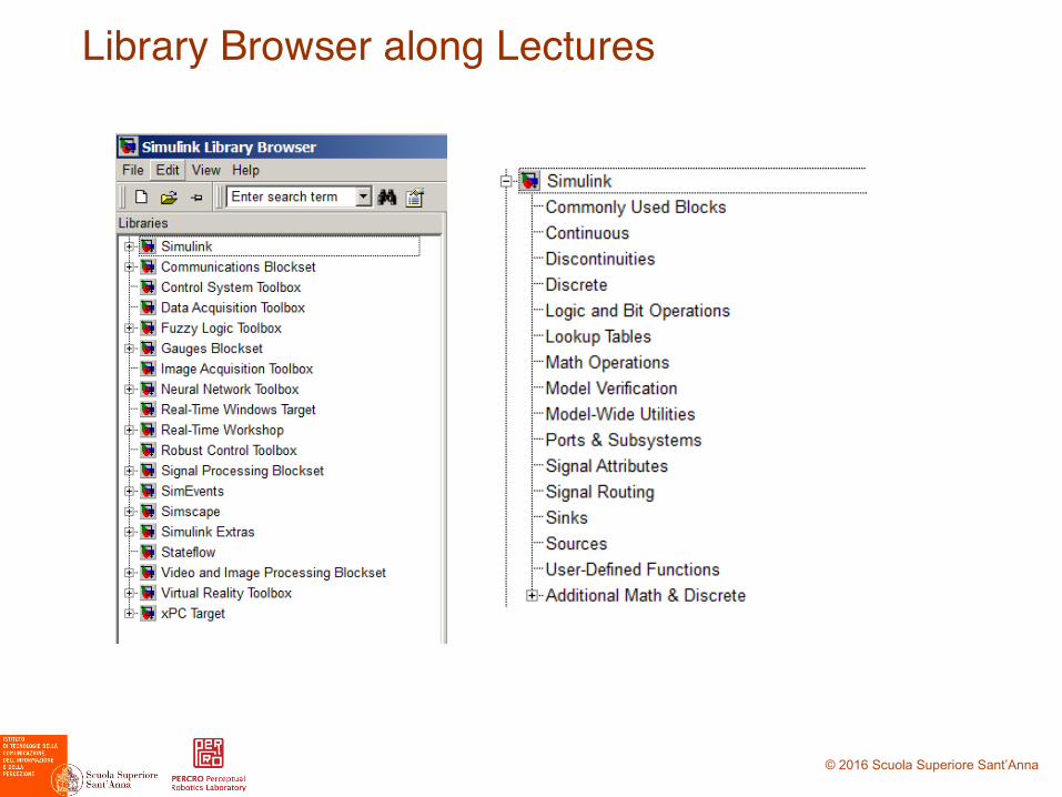
Simulink Library Browser
Search Block by Name and Description
Block list
Description
Library Tree
New Model (CTRL+N)
The library browser manages the available blocks
Explore it for understanding and finding solutions
© 2016 Scuola Superiore Sant’Anna
Library Browser along Lectures
© 2016 Scuola Superiore Sant’Anna
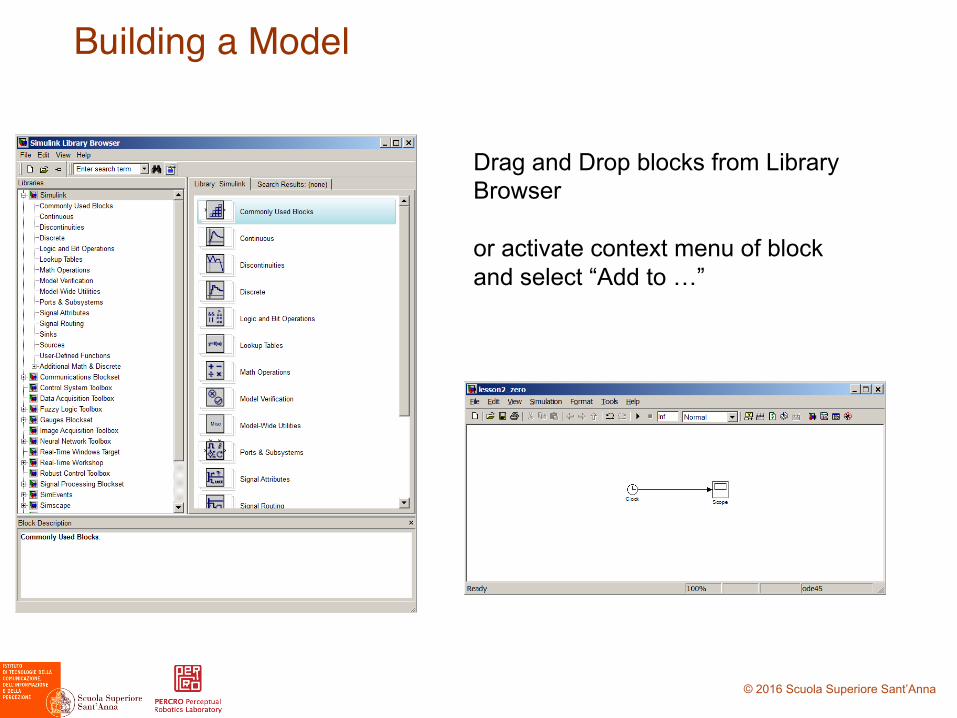
Building a Model
Drag and Drop blocks from Library Browser
or activate context menu of block and select “Add to …”

© 2016 Scuola Superiore Sant’Anna
Manipulating Blocks
• Selection• Multiple Selection with Shift• Multiple Selection with Box Selection
• Clone• Drag with CTRL
• Move Blocks• Drag• Rotate (CTRL+R)
• Connect Blocks• Select first and select second using CTRL/CMD• Branch line by holding CTRL from an existing line• Disconnect block by drag a block holding SHIFT

© 2016 Scuola Superiore Sant’Anna
Simulation
• Execution of the Simulation from startTime to stopTime times• Expressed in simulation seconds• Can be an expression• Can be up to Infinity (Inf)• Can be stopped by the “Stop Block”
• Simulation is decomposed in Time Steps as Fixed or Variable steps

© 2016 Scuola Superiore Sant’Anna
Running a Model
Pause/Stop
Current TimeStatus Integration Time
• Ex: Play with time step min/max• Try other function generators

© 2016 Scuola Superiore Sant’Anna
Invoking Simulation from Matlab
• The “sim” command allows to run a model from MATLAB changing parameters and input data– sim(modelname,param,paramvalue…)– sim(modelname,struct)
• Example Options– SimulationMode– SaveState– StateSaveName
• The model(..) command allows for finer control of the Simulation

© 2016 Scuola Superiore Sant’Anna
Looking at Results
• Insert Scope/Floating Scope/XY Graph• Context menu: Create and Connect Viewer
• Use Signal selector for modifying the signal
Signal selector
AutozoomZoom
Parameters
Properties

© 2016 Scuola Superiore Sant’Anna
Bouncing Ball - Integrator
• Integrates a differential equation
• Inputs and Ports– Input (always)– Reset– Initial Condition– Saturation– State

© 2016 Scuola Superiore Sant’Anna
Bouncing Ball
• This is an example of Continuous System with Simulink

© 2016 Scuola Superiore Sant’Anna
Bouncing Ballsldemo_bounce_two_integrators
© 2016 Scuola Superiore Sant’Anna
Heat Example
• From Mathworks website• https://it.mathworks.com/help/simulink/gs/define-system.html?s_cid=learn_doc

© 2016 Scuola Superiore Sant’Anna
Bacteria Example
• Birth rate = b x– b = 1/hour
• Death rate = p x2– p=0.5

© 2016 Scuola Superiore Sant’Anna
Exercise
• Create a 2D source (e.g. sin wave and )• Compute the polar coordinates (modulus and angle) and plot them

© 2016 Scuola Superiore Sant’Anna
Exercise
• Cannon Dynamics with bouncing• Ballistics with air resistance (1D)– Fd = -D v|v|– F = Fd – mg = ma
• Parameters– m=0.145kg– D=0.02– x0=(0,0)– v0=(0.1,0.2) m/s

© 2016 Scuola Superiore Sant’Anna
Exercise/2
• Based on the previous Simulation modify the initial conditions from Matlab and use the “sim” function to execute the simulation and collect the final end position

© 2016 Scuola Superiore Sant’Anna
Reference of Blocks in this Lecture
IC (initial value)Signal Attributes
Mux/DeMuxSignal Routing
SwitchSignal Routing
From/GoToSignal Routing
SelectorSignal Routing
ScopeSinks
DisplaySinks
STOPSinks
To WorkspaceSinks

© 2016 Scuola Superiore Sant’Anna
Reference of Blocks in this Lecture / 2
ConstantSources
GroundSources
Sine WaveSources
ClockSources
IntegratorContinuous
ComparisonLogical
GainMath
Product/SumMath
From WorkspaceSources
TrigonometricMath
SQRTMath