Concept Design and Performance Evaluation of a Fossil-Free ...

sustainability

Article

Concept Design and Performance Evaluation of aFossil-Free Operated Cargo Ship withUnlimited Range

Enric Julià, Fabian Tillig and Jonas W. Ringsberg *

Department of Mechanics and Maritime Sciences, Division of Marine Technology, Chalmers University ofTechnology, SE-412 96 Gothenburg, Sweden; [email protected] (E.J.); [email protected] (F.T.)* Correspondence: [email protected]; Tel.: +46-76-772-1489

Received: 12 July 2020; Accepted: 11 August 2020; Published: 15 August 2020��

Abstract: To meet the IMO goals of emissions reduction in shipping, drastic actions must betaken. Wind-assisted propulsion and renewable energy sources are today discussed frequently asrealistic alternatives for future ship propulsion and energy production. This study presents a newand innovative concept of a fossil-free operated cargo ship aiming to achieve an unlimited range.The purpose of the study is to present the feasibility but also the limitations of a ship propelledand operated purely on renewable energy harnessed at sea, independent from shore-based energysources. Aside from Flettner rotors for propulsion, the ship concept incorporates photovoltaicgenerators, wind turbines, and a dual-mode propeller to produce energy for the auxiliary systemsand for the Flettner rotors, as well as batteries to balance the energy production and consumption.The dual-mode propeller can be used for energy generation and propulsion, thus levelling out anyspeed drops or peaks and thereby ensuring more reliable operation. The whole system is modellednumerically, and full ship voyages are simulated using the ship performance model ShipCLEAN.Results show feasible achieved speeds on a route with realistic weather conditions. However, negativeenergy balances limit the pure renewable sailing conditions. Further logistic and technical challengesare discussed.

Keywords: fossil-free shipping; renewable energy; ship design; wind propulsion

1. Introduction

Global trade is one of the pillars of the modern world, where shipping stands for about 90%of the total cargo volume [1]. Today, ships are mainly powered by fossil fuels, and the combustionis responsible for the emission of pollutant gases such as NOx and SOx and about 3% of the totalCO2 emissions. Additionally, it is predicted that emissions will increase between 150–250% until2050 [2]. Climate change is the main effect caused by emissions and has already become a criticalsituation for society. In the last decades, renewable energies have been reintroduced in the shippingindustry. These energy sources have been incorporated mainly as a complementary technology,hybridizing traditional fossil fuel-powered systems, see e.g., [3–12], but some projects substitute fossilfuels completely [13].

Some studies have investigated the viability of using the wind to propel ships: [3,4] studied wingsails propulsion, [5] evaluated the application of Flettner rotors, and in [6,7] the benefits of using kitesfor propulsion were evaluated. In all these studies, the primary conclusion was that fuel consumptioncan be reduced by 20% to more than 30% for normal sailing conditions in merchant shipping. With thewind as an energy source, [8,9] considered wind turbines to generate electric power. This technologyreaches fuel savings of more than 35%, contributing to a relevant reduction of emissions. The study

Sustainability 2020, 12, 6609; doi:10.3390/su12166609 www.mdpi.com/journal/sustainability

http://www.mdpi.com/journal/sustainability

http://www.mdpi.com

https://orcid.org/0000-0001-6950-1864

http://www.mdpi.com/2071-1050/12/16/6609?type=check_update&version=1

http://dx.doi.org/10.3390/su12166609

http://www.mdpi.com/journal/sustainability

Sustainability 2020, 12, 6609 2 of 23

presented in [10] considered a set of solar panels and a battery system as a hybrid electric generator. It ishighlighted that the time zone and the local time are the parameters that mainly influence the energyproduction. In [11,12], the impact of installing a hydro turbine under the ship hull was investigated,showing energy savings of more than 3%. Finally, [13] studied the journey of a fossil-free ship withsails and wave-foils as the main power systems. It was concluded that the achievable speed for a routefrom Funchal to Punta Delgada was about 5–6 knots with a standard deviation of 4 knots.

The solutions and innovations presented in these studies show a positive impact of alternativepropulsion and renewable energies regarding the reduction of emissions and fuel cost. However, to keeptoday’s shipping schedules, more energy is often required than could be produced by renewablesources. This aspect has not been considered sufficiently in most recent research studies. Thus,the objective of this study is to define the benefits and limitations of a ship purely powered withrenewable energy systems by developing a reference concept vessel without fossil fuel technologiesand simulate its performance for different routes and weather conditions.

In Section 2, the method used in the study is presented together with the case study vessel.The section explains the modelling of renewable energy systems and its integration with the shipperformance prediction model ShipCLEAN to simulate journeys for different routes and weatherconditions. In the concept ship design process, ship dimensions and renewable energy systemcharacteristics are defined. Section 3 presents the results of different simulation cases to analyze howweather conditions and restrictions on ship speed influence voyage time and energy consumption.The conclusions of the study are presented in Section 4. The project focuses on the study of the technicaland practical feasibility of the installed technology; the economic viability of the project has not beenevaluated in the present work.

2. Concept Vessel and Methodology

In this section, a numerical model to calculate the ship speed, energy consumption, and energyproduction from an established set of renewable systems in a defined meteorological condition ispresented. The model was used to evaluate the performance of a ship in variable weather conditionsalong a route.

The study in [14] demonstrated the potential of the renewable systems used in the present work.Some assumptions have been made regarding the purpose and characteristics of the concept shipduring the selection of renewable technologies.

• Low-speed ship: It was assumed that the renewable power possible to obtain from systemsinstalled in a ship is reduced compared to the energetical density of a fossil fuel. This assumptionwas made when deciding the velocity considered as acceptable on the fossil-free operated shipconcept. From a previous study on pure renewable-powered ships ([13]), the speed considered asacceptable is between 5 and 6 knots average speed.

• High blockage hull: The low ship speed considered limits the ship cargo purpose to those shiptypes carrying cargo with low volume freight price. A high blockage ship hull was assumed forthe present study. A high blockage ship is referred to as a tanker ship or bulk carrier, which hasspeeds that stay in the range between 13 and 18 knots. It was assumed that corresponding speedreduction from a fossil-based to a fossil-free operated ship can be accepted by the market.

• Open deck space: As most of the current existing renewable technologies are installed in theweather deck area, the concept of ship design cannot require the open deck for cargo handlinglabors. Therefore, the ship type is limited to tanker ships, where cargo can be handled with pipes,or bulk carriers, in which cargo can be handled with side openings.

• Autonomous systems: The systems onboard must be designed to have the minimum impact onthe crew operation working autonomously or with minimum interaction.

Additionally, the current study aims to demonstrate the applicability of the ship performancemodel ShipCLEAN [15] to define and simulate the propulsion system of the fossil-free concept ship


with wind technologies as the main propulsor. From the ship dimensions, the wind propulsion systemcharacteristics and weather conditions, ShipCLEAN evaluated the equilibrium of forces and momentsin 4 degrees of freedom (surge, sway, yaw, and heel) and predicted the obtained ship speed andenergy demand for the rotors for pure sailing (see Section 2.1). With the same weather parameters,the power generation from wind turbines, solar panels, and a dual-mode propeller/hydro turbine inhydro turbines mode was calculated (see Section 2.2). To facilitate certain control of the speed duringthe journey, a parameter to limit the ship’s minimum speed was introduced in the model. If the attainedship speed in pure sailing mode was lower than the minimum speed, the hydro turbine turned topropeller mode to provide the additional thrust to achieve the minimum speed, using energy stored inbatteries (see Sections 2.1 and 2.2). The method focused on being open and generic to facilitate futuremodifications of routes and weather characteristics. The simulation procedure is presented in Figure 1.

Sustainability 2020, 12, x FOR PEER REVIEW 3 of 25

system characteristics and weather conditions, ShipCLEAN evaluated the equilibrium of forces and moments in 4 degrees of freedom (surge, sway, yaw, and heel) and predicted the obtained ship speed and energy demand for the rotors for pure sailing (see Section 2.1). With the same weather parameters, the power generation from wind turbines, solar panels, and a dual-mode propeller/hydro turbine in hydro turbines mode was calculated (see Section 2.2). To facilitate certain control of the speed during the journey, a parameter to limit the ship’s minimum speed was introduced in the model. If the attained ship speed in pure sailing mode was lower than the minimum speed, the hydro turbine turned to propeller mode to provide the additional thrust to achieve the minimum speed, using energy stored in batteries (see Sections 2.1 and 2.2). The method focused on being open and generic to facilitate future modifications of routes and weather characteristics. The simulation procedure is presented in Figure 1.

Figure 1. Flowchart of the simulation procedure.

2.1. Propulsion Systems

In this section, two wind propulsion systems (wing sails and Flettner rotors) are compared and evaluated. The VPP model ShipCLEAN was used to evaluate the main propulsion system, and a dual-mode propeller/hydro turbine was introduced as a support propulsion system while using propeller mode.

2.1.1. Flettner Rotors Versus Wing Sails

To select the most adequate wind propulsion system, it was required to compare the most feasible technologies currently available in the market. In this study, Flettner rotors and wing sails were compared. Both systems have pros and cons. This section motivates the selection of the most effective system according to the requirements of the concept ship.

Thrust and side force coefficients (𝐶( ) and 𝐶( ) respectively) are the parameters required to evaluate the forces generated by the sails. These parameters were used in Equations (1) and (2) to calculate the thrust and the side force of the ship (𝐹( ) and 𝐹( ), respectively). 𝐹( ) = 𝐶( ) × 𝐴 × 𝑛 × 𝜌2 × 𝑎𝑤𝑠 (1)

𝐹( ) = 𝐶( ) × 𝐴 × 𝑛 × 𝜌2 × 𝑎𝑤𝑠 (2)

where 𝐴 is the sail area, 𝑛 is the number of sails, 𝜌 is the density of the air, and 𝑎𝑤𝑠 is the apparent wind speed.

Figure 2 shows the value of the coefficients as a function of the apparent wind angle for a standard wing sail and a Flettner rotor. It was shown that the Flettner rotor produces higher forces in most of the conditions. This means that a wing sail always requires more sail area to generate the same thrust power (note that the sail area is the projected area of the cylinder or the sail).

Figure 1. Flowchart of the simulation procedure.

2.1. Propulsion Systems

In this section, two wind propulsion systems (wing sails and Flettner rotors) are compared andevaluated. The VPP model ShipCLEAN was used to evaluate the main propulsion system, and adual-mode propeller/hydro turbine was introduced as a support propulsion system while usingpropeller mode.

2.1.1. Flettner Rotors Versus Wing Sails

To select the most adequate wind propulsion system, it was required to compare the most feasibletechnologies currently available in the market. In this study, Flettner rotors and wing sails werecompared. Both systems have pros and cons. This section motivates the selection of the most effectivesystem according to the requirements of the concept ship.

Thrust and side force coefficients (C(t) and C(s) respectively) are the parameters required toevaluate the forces generated by the sails. These parameters were used in Equations (1) and (2) tocalculate the thrust and the side force of the ship (F(x) and F(y), respectively).

F(x) = C(t) ×A× n×ρ

2× aws2 (1)

F(y) = C(s) ×A× n×ρ

2× aws2 (2)

where A is the sail area, n is the number of sails, ρ is the density of the air, and aws is the apparentwind speed.

Figure 2 shows the value of the coefficients as a function of the apparent wind angle for a standardwing sail and a Flettner rotor. It was shown that the Flettner rotor produces higher forces in most of


the conditions. This means that a wing sail always requires more sail area to generate the same thrustpower (note that the sail area is the projected area of the cylinder or the sail).Sustainability 2020, 12, x FOR PEER REVIEW 4 of 25

Figure 2. Coefficients for Flettner rotor and wing sail [14].

The effect that these forces are producing when deciding to use Flettner rotors or wing sails in

the concept ship is the resultant effect in sailing equilibrium. In both cases, the thrust force follows a

similar pattern despite the higher values of rotors, with no production on for front winds, a peak in

the range between 90°–130°, and a considerable reduction for back winds. However, the change in

sailing behavior for the different systems is driven by the side forces.

In the case of wing sails, the side force appeared on the first range of speeds. From 0° to 55°, the

side forces are higher than thrust. Therefore, in this period, the ship gradually started the movement

with prominent drift. After 55°, the thrust increased while the side force started decreasing, achieving

at 90°–110° maximum thrust with lateral force close to 0, this being the best condition for navigation.

In the following range (110°–140°), the lateral force increased, but in a lower volume than thrust, so

the drift was reduced. Finally, in the last section up to back winds, the thrust was reduced, and the

lateral force was cancelled so that the drift was zero.

In the case where Flettner rotors were installed, in the first angles up to 65°, the side force was

higher than the thrust with a starting of the movement with strong drift. After this critical point, the

thrust force increased while the lateral force decreased, reaching the most optimal point at 110° when

the thrust was maximum, and the lateral force was zero (condition where there is no drift). Finally,

in the wind range from 110° to 180°, the lateral force increased while the thrust decreased, creating a

situation for back winds with prominent drift and reduced thrust.

The effect of the thrust and side force was further evaluated with the speed calculation of the

two different systems on an example vessel. Figure 3a shows a polar plot of the ship speed produced

by one wing sail of 1800 m2 of sail area (blue line) and a Flettner rotor of 150 m2 of sail area (pink line)

when the sails are individually installed in a high blockage hull with a length of 183 m [14]. The polar

plot was produced using the VPP model ShipCLEAN, with an optimization of the rpm/angle of attack

of the Flettner rotor and wing sail to achieve the highest possible ship speed. It was shown that with

a Flettner rotor, the ship experienced significant decreasing in front and back winds. Instead, wing

sails showed a more constant pattern for back winds.

Figure 2. Coefficients for Flettner rotor and wing sail [14].

The effect that these forces are producing when deciding to use Flettner rotors or wing sails inthe concept ship is the resultant effect in sailing equilibrium. In both cases, the thrust force follows asimilar pattern despite the higher values of rotors, with no production on for front winds, a peak in therange between 90◦–130◦, and a considerable reduction for back winds. However, the change in sailingbehavior for the different systems is driven by the side forces.

In the case of wing sails, the side force appeared on the first range of speeds. From 0◦ to 55◦,the side forces are higher than thrust. Therefore, in this period, the ship gradually started the movementwith prominent drift. After 55◦, the thrust increased while the side force started decreasing, achievingat 90◦–110◦ maximum thrust with lateral force close to 0, this being the best condition for navigation.In the following range (110◦–140◦), the lateral force increased, but in a lower volume than thrust, so thedrift was reduced. Finally, in the last section up to back winds, the thrust was reduced, and the lateralforce was cancelled so that the drift was zero.

In the case where Flettner rotors were installed, in the first angles up to 65◦, the side force washigher than the thrust with a starting of the movement with strong drift. After this critical point,the thrust force increased while the lateral force decreased, reaching the most optimal point at 110◦

when the thrust was maximum, and the lateral force was zero (condition where there is no drift).Finally, in the wind range from 110◦ to 180◦, the lateral force increased while the thrust decreased,creating a situation for back winds with prominent drift and reduced thrust.

The effect of the thrust and side force was further evaluated with the speed calculation of the twodifferent systems on an example vessel. Figure 3a shows a polar plot of the ship speed produced byone wing sail of 1800 m2 of sail area (blue line) and a Flettner rotor of 150 m2 of sail area (pink line)when the sails are individually installed in a high blockage hull with a length of 183 m [14]. The polarplot was produced using the VPP model ShipCLEAN, with an optimization of the rpm/angle of attackof the Flettner rotor and wing sail to achieve the highest possible ship speed. It was shown that with aFlettner rotor, the ship experienced significant decreasing in front and back winds. Instead, wing sailsshowed a more constant pattern for back winds.

Figure 3b shows the pattern of power consumption of the same example Flettner rotor. It isremarkable that in those angles where there is an extreme side force (50◦ and 180◦), the consumptionrose drastically to reach the optimum rotational speed.

Achieved speeds from Figure 3 show that for the two evaluated sails there was a higher thrustfrom a single wing sail than for a single Flettner rotor. However, from a practical point of view thesail area of the wing sail is twelve times bigger than the Flettner rotor; thus, the comparison is notdeterminant. Further research from [16] simulated two different routes for a tanker ship and comparedthe fuel savings when Flettner rotors or wing sails were installed onboard as wind-assisted propulsion


systems. The result of the study showed that fuel savings using Flettner rotors are slightly higher thanusing wing sails (0.1–0.4% higher), even considering the power required to spin the rotors.Sustainability 2020, 12, x FOR PEER REVIEW 5 of 25

(a) (b)

Figure 3. (a) Ship speeds polar plot for a high blockage ship powered with wind power systems for

10 m/s wind speed [14]; pink line: speed with one Flettner rotor (A = 150 m2); blue line: speed with

one wing sail (A = 1800 m2); (b) Power consumption of a single Flettner (A = 150 m2) for 10 m/s wind

speed and optimized rotational speed [14].

Figure 3b shows the pattern of power consumption of the same example Flettner rotor. It is

remarkable that in those angles where there is an extreme side force (50° and 180°), the consumption

rose drastically to reach the optimum rotational speed.

Achieved speeds from Figure 3 show that for the two evaluated sails there was a higher thrust

from a single wing sail than for a single Flettner rotor. However, from a practical point of view the

sail area of the wing sail is twelve times bigger than the Flettner rotor; thus, the comparison is not

determinant. Further research from [16] simulated two different routes for a tanker ship and

compared the fuel savings when Flettner rotors or wing sails were installed onboard as wind-assisted

propulsion systems. The result of the study showed that fuel savings using Flettner rotors are slightly

higher than using wing sails (0.1–0.4% higher), even considering the power required to spin the

rotors.

To evaluate and motivate the most suitable wind propulsion technology for the project, other

factors than the achievable ship speed must be considered. From a practical point of view,

autonomous control of the system is essential. Flettner rotors are easier to operate as the rotational

speed is the only parameter that needs to be adjusted for maximum efficiency; cf. [14,17]. It is also

necessary to reduce negative interactions of the sail with other renewable systems. Due to the smaller

required sail area, Flettner rotors are more suitable to save space and reduce negative interaction with

other systems, e.g., solar panels ([14,18]).

Flettner rotors have been selected in the study as the main propulsion system for their high

efficiency in real environmental conditions, their flexibility and simplicity in operation, and their

small sail area that reduces their interference with other renewable technologies on deck.

Additionally, the ShipCLEAN model has already been validated proving reliable results using

Flettner rotors as a wind-assisted propulsion system [15].

2.1.2. The ShipCLEAN Model

ShipCLEAN is a ship performance prediction model developed to estimate the energy

consumption of a vessel based on a limited number of required inputs. The design of the model has

an open format to enable simulations for different ship types and weather conditions. It was

developed and prepared for the possibility to include wind-assisted propulsion to present the

Figure 3. (a) Ship speeds polar plot for a high blockage ship powered with wind power systems for10 m/s wind speed [14]; pink line: speed with one Flettner rotor (A = 150 m2); blue line: speed withone wing sail (A = 1800 m2); (b) Power consumption of a single Flettner (A = 150 m2) for 10 m/s windspeed and optimized rotational speed [14].

To evaluate and motivate the most suitable wind propulsion technology for the project, other factorsthan the achievable ship speed must be considered. From a practical point of view, autonomouscontrol of the system is essential. Flettner rotors are easier to operate as the rotational speed is the onlyparameter that needs to be adjusted for maximum efficiency; cf. [14,17]. It is also necessary to reducenegative interactions of the sail with other renewable systems. Due to the smaller required sail area,Flettner rotors are more suitable to save space and reduce negative interaction with other systems, e.g.,solar panels ([14,18]).

Flettner rotors have been selected in the study as the main propulsion system for their highefficiency in real environmental conditions, their flexibility and simplicity in operation, and their smallsail area that reduces their interference with other renewable technologies on deck. Additionally,the ShipCLEAN model has already been validated proving reliable results using Flettner rotors as awind-assisted propulsion system [15].

2.1.2. The ShipCLEAN Model

ShipCLEAN is a ship performance prediction model developed to estimate the energy consumptionof a vessel based on a limited number of required inputs. The design of the model has an open format toenable simulations for different ship types and weather conditions. It was developed and prepared forthe possibility to include wind-assisted propulsion to present the positive influence that wind energycan have in the maritime market, see [18] for detailed information. In the current study, the model wasused to evaluate the performance of a ship with wind power as the main propulsion system.

To predict the ship’s performance, the model is designed to follow the process in Figure 4.ShipCLEAN requires some static inputs, i.e., ship design characteristics (main dimensions, designspeed, ship type, and propeller dimensions), dynamic inputs as the weather parameters (wind speedand direction, currents and water temperature), and wind technology characteristics (sail area, numberof sails, thrust coefficient, and side coefficient).



positive influence that wind energy can have in the maritime market, see [18] for detailed information. In the current study, the model was used to evaluate the performance of a ship with wind power as the main propulsion system.

To predict the ship’s performance, the model is designed to follow the process in Figure 4. ShipCLEAN requires some static inputs, i.e., ship design characteristics (main dimensions, design speed, ship type, and propeller dimensions), dynamic inputs as the weather parameters (wind speed and direction, currents and water temperature), and wind technology characteristics (sail area, number of sails, thrust coefficient, and side coefficient).

The static part of the model uses empirical formulations to convert the basic ship dimensions into a set of detailed parameters that define hull shape, stability, and resistance (calm water resistance and air resistance). Results from the static part are then used for the dynamic analysis where, together with the weather characteristics and the sail system dimensions, a balance of applied forces is evaluated for 4 degrees of freedom (DOF). According to [17], the analysis for 4 DOF (surge, sway, yaw, and heel) in the balance of forces is a requirement when using wind power propulsion in a ship. For this type of analysis, the forces and moments that take place are divided into aerodynamic (mainly consistent in the wind-assisted system but also other structures above the waterline) and hydrodynamic (underwater structures such as the hull and rudder are analyzed against the water flow). The center of forces is then defined as the point where lift and drag are applied. As the aerodynamic and hydrodynamic forces have their center of forces in a different longitudinal point of the ship, a yaw moment is generated, which must be compensated by the rudder.

Figure 4. Schematic view of ShipCLEAN system model [18].

The method used in ShipCLEAN to simulate the behavior of Flettner rotors has been designed to give highly accurate results. Interaction effects between sails and other elements of the vessel have relevant attention on the simulation model design. Aerodynamic interaction effects are modelled considering the influence of multiple rotors on the ship, and the vertical wind speed distribution is simulated. The optimal rpm of the rotors is found by optimizing the individual rpm for best performance considering power consumption and added resistance from drift and rudder. The induced speeds and resulting local wind speeds and angles for a ship with four rotors are shown in Figure 5. Additionally, a parameter defining the maximum allowed power consumption of the rotors is introduced. In this case, the conditions were re-optimized; see [15,17] for details. In the current study, ShipCLEAN was used to predict ship speed and Flettner rotor power consumption, respecting 4 DOF.

Figure 4. Schematic view of ShipCLEAN system model [18].

The static part of the model uses empirical formulations to convert the basic ship dimensions intoa set of detailed parameters that define hull shape, stability, and resistance (calm water resistance andair resistance). Results from the static part are then used for the dynamic analysis where, together withthe weather characteristics and the sail system dimensions, a balance of applied forces is evaluated for4 degrees of freedom (DOF). According to [17], the analysis for 4 DOF (surge, sway, yaw, and heel) inthe balance of forces is a requirement when using wind power propulsion in a ship. For this type ofanalysis, the forces and moments that take place are divided into aerodynamic (mainly consistent in thewind-assisted system but also other structures above the waterline) and hydrodynamic (underwaterstructures such as the hull and rudder are analyzed against the water flow). The center of forces is thendefined as the point where lift and drag are applied. As the aerodynamic and hydrodynamic forceshave their center of forces in a different longitudinal point of the ship, a yaw moment is generated,which must be compensated by the rudder.

The method used in ShipCLEAN to simulate the behavior of Flettner rotors has been designed togive highly accurate results. Interaction effects between sails and other elements of the vessel haverelevant attention on the simulation model design. Aerodynamic interaction effects are modelledconsidering the influence of multiple rotors on the ship, and the vertical wind speed distribution issimulated. The optimal rpm of the rotors is found by optimizing the individual rpm for best performanceconsidering power consumption and added resistance from drift and rudder. The induced speeds andresulting local wind speeds and angles for a ship with four rotors are shown in Figure 5. Additionally,a parameter defining the maximum allowed power consumption of the rotors is introduced. In thiscase, the conditions were re-optimized; see [15,17] for details. In the current study, ShipCLEAN wasused to predict ship speed and Flettner rotor power consumption, respecting 4 DOF.Sustainability 2020, 12, x FOR PEER REVIEW 7 of 25

Figure 5. Induced velocities in an array of four Flettner rotors [15].

2.1.3. Dual-Mode Propeller/Hydro Turbine (Propeller Mode)

The dual-mode propeller/hydro turbine is ideated as a system that, in propeller mode, generates thrust when sail propulsion does not provide enough thrust to achieve the minimum ship speed. In conditions when the propeller mode is not required, it can make use of the water flow through the blades to generate electricity as a hydro turbine. Considering these operational conditions, the hydro turbine is always working in the highest range of ship speeds, while the propeller mode is used in the lowest range of speeds to reach the minimum required ship speed.

The system, not common yet in the market, has been previously studied and simulated in [11] as an efficient energy source for wind propelled ships. The study evaluated three different propellers with different pitch ratios. In all cases, it was shown that, even for low speeds, the system produced high power showing technical viability.

The design of this propeller with double functionality is a challenge, as it must work in both propeller and turbine mode. The propeller was designed using the Matlab open-source code “OpenProp” [19] by optimizing a profile “NACA 65A010”. The parameters that have been evaluated in the process were the camber, the ship speed design, and the design RPMs of the propeller. The rest of the parameters were optimized automatically for each case. The optimization was done to have a good relation of power coefficient and drag coefficient for hydro turbine mode and a maximum peak of propeller efficiency for propeller mode. For the calculation of the thrust in propeller mode, propeller curves were obtained from “OpenProp”. The curves required were the thrust coefficient (KT) and the efficiency (EFFY) of the propeller shown in Figure 6.

Figure 6. Propeller coefficient curves from “OpenProp”.

The calculation of the power consumption of the propeller to reach the minimum speed defined was evaluated with Equation (3) [11]:

0.5 1 1.5 2Js (advance coefficient)

-0.2

0

0.2

0.4

0.6

0.8

1

KT ,

EFFY

KTEFFY



The dual-mode propeller/hydro turbine is ideated as a system that, in propeller mode, generatesthrust when sail propulsion does not provide enough thrust to achieve the minimum ship speed.In conditions when the propeller mode is not required, it can make use of the water flow through theblades to generate electricity as a hydro turbine. Considering these operational conditions, the hydro


turbine is always working in the highest range of ship speeds, while the propeller mode is used in thelowest range of speeds to reach the minimum required ship speed.

The system, not common yet in the market, has been previously studied and simulated in [11] asan efficient energy source for wind propelled ships. The study evaluated three different propellerswith different pitch ratios. In all cases, it was shown that, even for low speeds, the system producedhigh power showing technical viability.

The design of this propeller with double functionality is a challenge, as it must work in bothpropeller and turbine mode. The propeller was designed using the Matlab open-source code“OpenProp” [19] by optimizing a profile “NACA 65A010”. The parameters that have been evaluatedin the process were the camber, the ship speed design, and the design RPMs of the propeller. The restof the parameters were optimized automatically for each case. The optimization was done to have agood relation of power coefficient and drag coefficient for hydro turbine mode and a maximum peakof propeller efficiency for propeller mode. For the calculation of the thrust in propeller mode, propellercurves were obtained from “OpenProp”. The curves required were the thrust coefficient (KT) and theefficiency (EFFY) of the propeller shown in Figure 6.




The dual-mode propeller/hydro turbine is ideated as a system that, in propeller mode, generates thrust when sail propulsion does not provide enough thrust to achieve the minimum ship speed. In conditions when the propeller mode is not required, it can make use of the water flow through the blades to generate electricity as a hydro turbine. Considering these operational conditions, the hydro turbine is always working in the highest range of ship speeds, while the propeller mode is used in the lowest range of speeds to reach the minimum required ship speed.

The system, not common yet in the market, has been previously studied and simulated in [11] as an efficient energy source for wind propelled ships. The study evaluated three different propellers with different pitch ratios. In all cases, it was shown that, even for low speeds, the system produced high power showing technical viability.

The design of this propeller with double functionality is a challenge, as it must work in both propeller and turbine mode. The propeller was designed using the Matlab open-source code “OpenProp” [19] by optimizing a profile “NACA 65A010”. The parameters that have been evaluated in the process were the camber, the ship speed design, and the design RPMs of the propeller. The rest of the parameters were optimized automatically for each case. The optimization was done to have a good relation of power coefficient and drag coefficient for hydro turbine mode and a maximum peak of propeller efficiency for propeller mode. For the calculation of the thrust in propeller mode, propeller curves were obtained from “OpenProp”. The curves required were the thrust coefficient (KT) and the efficiency (EFFY) of the propeller shown in Figure 6.


The calculation of the power consumption of the propeller to reach the minimum speed defined was evaluated with Equation (3) [11]:

0.5 1 1.5 2Js (advance coefficient)

-0.2

0

0.2

0.4

0.6

0.8

1

KT ,

EFFY

KTEFFY


The calculation of the power consumption of the propeller to reach the minimum speed definedwas evaluated with Equation (3) [11]:

Pprop = ∆T vship ηprop ηmot (3)

where ∆T is the increment of thrust needed to reach the minimum required speed, vmin, vship is thespeed reached by the ship making use of the propeller (corresponding to vmin), ηprop is the propellerefficiency from OpenProp curves, and ηmot is the efficiency of the electric motor set as a constant valueof 95% [11,20].

2.1.4. Speed Limit and Velocity Made Good (VMG)

The speed limit was introduced into the simulation model to control the sailing performance on aroute. The limitation is defined by a minimum speed (vmin). If the pure sailing propulsion does notgive enough thrust to reach vmin, the dual-mode propeller/hydro turbine will provide additional thrust.

The performance of wind propulsion is highly dependent on the wind angle and speed.Thus, wind-powered vessels require an adapted trip plan, depending on the wind characteristics.


The adaptation was done by the velocity made good (VMG) optimization function. This functionavoids conditions where no wind thrust is produced and optimizes the deviation angles (tacks) formaximum speed towards the target. Under regular, pure wind propulsion conditions, the VMGfunction evaluated the Flettner rotor performance and ship resistance from ShipCLEAN for differentdeviation angles from the direct course. The optimal condition was obtained as the maximum VMG byprocessing the ship speeds and deviation angles, see [14] for details.

In conditions where the total thrust is partly produced by the propeller (because vmin cannot bereached with pure sailing), the optimization function calculated the angle that requires the lowestenergy consumption to reach a VMG equal to vmin. vmin is always considered in the VMG function.This means that although the real ship speed accomplishes the limit, VMG is the speed that needs to beabove the limit considering the deviation angles.

2.2. Power Energy System

A challenging aspect of the study is the generation of energy onboard. The configuration ofrenewable technologies must be optimal for maximum energy production. In the former study [14],the strength and disadvantages of some of the most developed renewable systems in the market wereshown. A basic diagram of the systems energy flow considered in this study is shown in Figure 7.The figure shows the energetical connections of the system. The electrical consumers are divided intotwo groups, the propulsion systems and the non-propulsive systems. The first group is explainedin Section 2.1. The non-propulsive systems group compromises all the additional consumers tooperate the ship, like machinery, governance, navigation, communication, and habitability. The electricproducers evaluated were the renewable systems installed onboard. The considered systems werevertical axis wind turbines, PV solar panels, and the turbine mode of the dual-mode propeller-hydroturbine, all of them highly dependent on weather conditions. Finally, to balance the power in thoseconditions where there is a surplus or insufficient power, the concept was supported by a batterystorage system. This section presents a summary of the electric producers and battery systems andhow they were implemented and coupled with ShipCLEAN.Sustainability 2020, 12, x FOR PEER REVIEW 9 of 25

Figure 7. System power structure diagram.

2.2.1. Wind Turbine

The vertical axis wind turbine was motivated due to its stability and functionality reasons, see [14] for details. The system has the function to generate electrical energy from the wind, which is used directly or stored in batteries. The wind turbine model assumes conditions of constant wind speed and direction for a fixed period, then, energy production is constant. The power generated by the wind turbine was calculated according to Equation (4): 𝑃 = 0.5 𝐶𝑝 𝜌 𝜂 𝐴 𝑣 (4)

where 𝐶𝑝 is the power coefficient from [21] shown in Figure 8, a factor that determines the conversion efficiency from the wind to the electrical generator. 𝜌 is the density of the air, and 𝜂 is the efficiency of the generator (assumed in [21] as 85%). 𝐴 is the area of the turbine, i.e., the length of the blades multiplied by the diameter of the rotor, and 𝑣 is the wind speed.

Figure 8. Power coefficient of wind turbines versus tip speed ratio from [21]. Cp represents the power coefficient and 𝜆 the tip speed ratio (𝜆 = tip speed of the turbine/wind speed).

The wind turbine has three reference speeds: minimum, nominal, and a cut-off speed. The minimum speed corresponds to the minimum wind speed required for the generator to start producing energy. Once the generator surpasses this limit, it increases its production until the wind speed is equal to the nominal wind speed where the production efficiency is maximum (from Figure 8, λ ≈ 4). Above the nominal speed, the rotational speed is maintained with the same power coefficient


2.2.1. Wind Turbine

The vertical axis wind turbine was motivated due to its stability and functionality reasons, see [14]for details. The system has the function to generate electrical energy from the wind, which is useddirectly or stored in batteries. The wind turbine model assumes conditions of constant wind speed and


direction for a fixed period, then, energy production is constant. The power generated by the windturbine was calculated according to Equation (4):

Pwind = 0.5 Cpwind ρair ηwind Awind vwind3 (4)

where Cpwind is the power coefficient from [21] shown in Figure 8, a factor that determines theconversion efficiency from the wind to the electrical generator. ρair is the density of the air, and ηwind isthe efficiency of the generator (assumed in [21] as 85%). Awind is the area of the turbine, i.e., the lengthof the blades multiplied by the diameter of the rotor, and vwind is the wind speed.



2.2.1. Wind Turbine

The vertical axis wind turbine was motivated due to its stability and functionality reasons, see [14] for details. The system has the function to generate electrical energy from the wind, which is used directly or stored in batteries. The wind turbine model assumes conditions of constant wind speed and direction for a fixed period, then, energy production is constant. The power generated by the wind turbine was calculated according to Equation (4): 𝑃 = 0.5 𝐶𝑝 𝜌 𝜂 𝐴 𝑣 (4)

where 𝐶𝑝 is the power coefficient from [21] shown in Figure 8, a factor that determines the conversion efficiency from the wind to the electrical generator. 𝜌 is the density of the air, and 𝜂 is the efficiency of the generator (assumed in [21] as 85%). 𝐴 is the area of the turbine, i.e., the length of the blades multiplied by the diameter of the rotor, and 𝑣 is the wind speed.

Figure 8. Power coefficient of wind turbines versus tip speed ratio from [21]. Cp represents the power coefficient and 𝜆 the tip speed ratio (𝜆 = tip speed of the turbine/wind speed).

The wind turbine has three reference speeds: minimum, nominal, and a cut-off speed. The minimum speed corresponds to the minimum wind speed required for the generator to start producing energy. Once the generator surpasses this limit, it increases its production until the wind speed is equal to the nominal wind speed where the production efficiency is maximum (from Figure 8, λ ≈ 4). Above the nominal speed, the rotational speed is maintained with the same power coefficient

Figure 8. Power coefficient of wind turbines versus tip speed ratio from [21]. Cp represents the powercoefficient and λ the tip speed ratio (λ = tip speed of the turbine/wind speed).

The wind turbine has three reference speeds: minimum, nominal, and a cut-off speed.The minimum speed corresponds to the minimum wind speed required for the generator to startproducing energy. Once the generator surpasses this limit, it increases its production until the windspeed is equal to the nominal wind speed where the production efficiency is maximum (from Figure 8,λ ≈ 4). Above the nominal speed, the rotational speed is maintained with the same power coefficientand a constant energy generation. When the wind reaches the cut-off speed, the turbine stops for safetyreasons, and energy production becomes zero. The current numerical model does not consider thedrag force generated by the turbine, as it is assumed to have a low impact considering the total shipresistance and forces generated by the Flettner rotors [8].

2.2.2. Solar Panels

Solar panels were placed on the weather deck of the concept ship covering the free available area.Photovoltaic installation is a system that requires an extensive open area to generate the amount ofpower demanded by a vessel. As is discussed in the assumptions from Section 2, a ship that requires theopen deck to handle the cargo is not considered in the present study. It is assumed that the placement ofthe panels does not interfere with the ship operation or other systems onboard. The energy productionof the solar panels was calculated using Equation (5); see [10,22,23].

PPV(t) = ηpv Apv I(t) (5)

where I(t) is the solar radiation intensity, Apv is the area of the solar panels, and ηpv is the efficiency fordifferent generation parameters. The efficiency ηpv is defined by Equation (6):

ηpv = ηre f(1− β

(Tc − Tre f

))ηconv (6)


where ηre f is the reference efficiency determined by the manufacturer, β is the temperature coefficientof the cell material, Tre f is the cell reference temperature, Tc is the photovoltaic (PV) cell temperature,and ηconv refers to other conversion loses from radiation to electric energy independent of the installation.The losses considered for solar panels with regular leaning and maintenance are the module degradationloss of 1%, dust and salt losses of 2%, reflection loses of 2.5%, and other electrical losses of 4% from thepanel to the main bus of the grid [24,25]. Note that the current model does not account for shadowlosses. Apv is the area of the PV surface defined in Equation (7). It is defined as the number of panels, n,multiplied by the area of each panel, Apanel.

Apv = n Apanel (7)

The solar radiation intensity, I(t), received by the photovoltaic panel surface was calculatedaccording to Equation (8). The parameter IB,N denotes the direct radiation perpendicular to the surfacedefined by the weather data. θ is the angle between the board and the solar rays, φ is the tilt anglefrom the horizontal surface, χ is the zenith angle or angle between the sun, and the vertical and ρ is theAlbedo or reflection index ([10,23]).

I(t) = IB,N

(cos(θ) + cos2

(φ

2

)sin(χ) +ρ cos(χ) sin2

(φ

2

))(8)

2.2.3. Dual-Mode Propeller/Hydro Turbine (Hydro Turbine)

Numerical calculations of the propeller-hydro turbine system were evaluated from the resultsobtained in the open code “OpenProp” [18]. The simulation of the hydro turbine generation systemrequired from “Open Prop” the turbine curves of the drag coefficient (CD) and power coefficient(CPH/T) shown in Figure 9. The curves were used to calculate the power generation and drag force ofthe propeller by using the Equations (9) and (10):

P =12

CPH/T ρwater Aprop vship3 ηH/T (9)

Fdrag = 0.5 CD ρwater vship2 Aprop (10)

where ρwater is the water density, Aprop is the circular propeller area, vship is the ship velocity, and ηH/Tare the efficiencies of the gearbox and the generator, set to 89% [11,26].


Figure 9. Hydro turbine coefficient curves from “OpenProp”.

The hydro turbine function starts working when the ship speed produced with wind propulsion reaches the minimum allowed speed. At this point, the power supply to the propeller stops, and the propeller starts a free rotating movement caused by the water flow through the blades. The free rotation is referred to the lowest value of drag coefficient, but as the torque from the electric generator is not applied, CD is zero, and the generation of electric power is zero (as a reference, this point is defined in Figure 9 as Phase 1). From the first condition, if the thrust from the sails increases, torque to the generator is applied, reducing the rotational speed of the propeller and increasing its advance coefficient (J) that results in a higher CP and CD that maintain the ship to the minimum ship speed and increase the power production (defined as Phase 2 in Figure 9). The advance coefficient increases with the sails’ thrust to the point where CP reaches its maximum. Then CD and CP stay stable independently of the thrust. In this condition, the ship speed increases with the maximum power coefficient (represented as Phase 3 in Figure 9).

2.2.4. Batteries

In the concept ship model, battery functions control the energy distribution around the ship by storing the surplus of the energy generation or by supplying energy to the ship consumers when not enough power is produced. If the global power balance is positive, the charging battery function is activated. With this mode, the system first stores the energy from DC producers as PV panels, and afterwards, the AC generators as hydro turbines and wind turbines as it optimizes the electric conversions. For this system, charging efficiency of 85% was assumed [27].

The discharging battery function is used when the power balance is negative. For this case, if the ship speed is higher than the minimum velocity requirement, the model reduces the delivered power for the Flettner rotors adapting the ship speed to 𝑣 . If the ship reaches 𝑣 and the power balance is still negative, the discharging battery function uses the energy stored in the batteries to fulfil the demand. For the energy discharging from the batteries, the efficiency is assumed to be 85% [27].

If additional energy is required, and all the energy produced by renewable systems and stored is already used, additional energy is required to fulfil the demand. It was assumed that shore-based electricity is stored in the batteries before the start of the trip. It was also assumed that there are always enough batteries in the ship. The resulting energy balance from route simulations defines the necessary number of batteries.

0.6 0.8 1 1.2 1.4 1.6 1.8Js (advance coefficient)

0

0.1

0.2

0.3

0.4

0.5

0.6

0.7

0.8

CP

, CD

Phase 1 Phase 2 Phase 3

CPCD

Figure 9. Hydro turbine coefficient curves from “OpenProp”.


The hydro turbine function starts working when the ship speed produced with wind propulsionreaches the minimum allowed speed. At this point, the power supply to the propeller stops, and thepropeller starts a free rotating movement caused by the water flow through the blades. The freerotation is referred to the lowest value of drag coefficient, but as the torque from the electric generatoris not applied, CD is zero, and the generation of electric power is zero (as a reference, this pointis defined in Figure 9 as Phase 1). From the first condition, if the thrust from the sails increases,torque to the generator is applied, reducing the rotational speed of the propeller and increasing itsadvance coefficient (J) that results in a higher CP and CD that maintain the ship to the minimum shipspeed and increase the power production (defined as Phase 2 in Figure 9). The advance coefficientincreases with the sails’ thrust to the point where CP reaches its maximum. Then CD and CP staystable independently of the thrust. In this condition, the ship speed increases with the maximumpower coefficient (represented as Phase 3 in Figure 9).

2.2.4. Batteries

In the concept ship model, battery functions control the energy distribution around the ship bystoring the surplus of the energy generation or by supplying energy to the ship consumers when notenough power is produced. If the global power balance is positive, the charging battery functionis activated. With this mode, the system first stores the energy from DC producers as PV panels,and afterwards, the AC generators as hydro turbines and wind turbines as it optimizes the electricconversions. For this system, charging efficiency of 85% was assumed [27].

The discharging battery function is used when the power balance is negative. For this case, if theship speed is higher than the minimum velocity requirement, the model reduces the delivered powerfor the Flettner rotors adapting the ship speed to vmin. If the ship reaches vmin and the power balanceis still negative, the discharging battery function uses the energy stored in the batteries to fulfil thedemand. For the energy discharging from the batteries, the efficiency is assumed to be 85% [27].

If additional energy is required, and all the energy produced by renewable systems and storedis already used, additional energy is required to fulfil the demand. It was assumed that shore-basedelectricity is stored in the batteries before the start of the trip. It was also assumed that there are alwaysenough batteries in the ship. The resulting energy balance from route simulations defines the necessarynumber of batteries.

2.3. Environmental Conditions

An accurate definition of the weather condition is essential to estimate realistic ship behavior andtrustable results. The process to generate the environmental conditions starts from average weatherdata source provided by [28]. It is based on global historical data from 1983 to the present. It is definedin a grid of 0.5 × 0.5 degrees covering all of the surface of the planet, and it gives the result for eachmonth of the year. Within this data source, it is defined as the mean value and the variance of windspeed and direction, solar radiation, and temperature.

To mimic realistic weather conditions, the average data must be converted to include variation intime, although the continuous variation would create an infinite number of calculations. The mostpractical and accurate way to deal with this is to define a period when the weather variables areassumed to be constant. In this study, it was set as one hour.

For each period, the weather values changes. The mean and variance of each weather parameterwere used in Monte Carlo simulations to generate random weather variables assuming Weibulldistributions for the wind speed and Normal distributions for the wind angle, solar radiation andtemperature. As this process was done to obtain the time at sea, and uncertainties in weather data arecrucial for the results, a total of 100 random values for each weather variable were generated.

The process starts when the ship enters a square of the grid and average data is defined, the randomvalues are generated, and the simulation calculates results for the sequence of random values with the


time advance. When the ship reaches the end of a square, new random values are generated with thenew average data. This process is continued until the end of the voyage.

2.4. Concept Ship

2.4.1. Ship Characteristics

The 183 m length high blockage ship (with block coefficient of 0.80) previously studied in [14]was used in this study. The ship characteristics are defined in Table 1.

Table 1. Concept ship dimensions.

Ship Dimension Value

LOA (Length Overall) 183 mDraft 11 m

Breadth 32.2 mDisplacement 50,618 t

Renewable systems weight 1050–1520 tBlock coefficient 0.80

The vessel is equipped with six Flettner rotors (5 × 30 m), a dual-mode propeller/hydro turbine,two vertical axis wind turbines, and 1564 solar panels. A schematic of the concept ship with thesystem distribution is shown in Figure 10. The energy consumption for the propulsive systems wascalculated with the simulation model, while the non-propulsive consumption was estimated fromprevious studies. According to [29], a ship with the previously mentioned characteristics duringsailing condition has 153.9 kW power demand from machinery services, 11 kW power demand fromgovernance service, 20 kW power demand from navigation assistance and communication service,and 41.9 kW power demand from habitability service. In total, it was considered that the powerconsumption while sailing is 226.8 kW. It was assumed that the power demand is constant during allthe simulation. A weight evaluation was done to see the influence of renewable systems on ship loads.The total added weight on the ship is in the range between 1050 and 1520 tons, which corresponds to2–3% of the total ship displacement [30–32]. Considering that the weight of the fossil fuel machineryand the fuel are removed, it is assumed that the weight increment produced can be easily balancedwith cargo weight reduction.Sustainability 2020, 12, x FOR PEER REVIEW 13 of 25

Figure 10. Schematic of the concept ship.

2.4.2. Flettner Rotors

Six Flettner rotors are symmetrically positioned on both sides of the ship (three on each side). Each rotor is 30 m high and 5 m in diameter. The rotors are installed in the front of the ship to advance the center of forces. An advanced position of the rotors, and the high side forces of the Flettner systems, are proved to give the most adequate drift condition for the studied ship to maximize the range of wind angles that the ship is able to sail and to minimize the required rudder angle for each sailing condition [15]. The previous studies [14,15] demonstrated that the configuration established with the respective rotor dimension is the most beneficial, assuming the attained speeds and energetical efficiency as the most critical aspects.

2.4.3. Vertical Wind Turbine

Two vertical axis wind turbines with three 13 m long blades, a rotor diameter of 15 m, and a nominal power generation of 70 kW were installed. The reference wind speeds for the turbine are 3 m/s as the minimum wind speed, 12 m/s of nominal wind speed and 26 m/s cut-off speed; see [8,21].

2.4.4. Photovoltaic Solar Panels

Solar panels cover the whole weather deck. There is a total of 1780 solar panels with an area of 2.16 m2, a nominal power of 460 W each, and a panel efficiency of 21.3%. The supporting structures for the panels were not considered, but it is assumed that these structures do not interfere with the crew operations.

2.4.5. Dual-Mode Propeller/Hydro Turbine

The system is composed of one propeller / hydro turbine with a diameter of 4 m and four blades. The propeller is designed for good performance in propeller mode below a 𝑣 of 5 knots speed and for good turbine mode above that speed. The optimization process gave as the optimum result a propeller without camber with its maximum efficiency rotating with an advance coefficient of 1.4. The propeller and turbine diagrams are shown in Figures 6 and 9. A 3D model of the propeller used is shown in Figure 11.

Figure 10. Schematic of the concept ship.


2.4.2. Flettner Rotors

Six Flettner rotors are symmetrically positioned on both sides of the ship (three on each side).Each rotor is 30 m high and 5 m in diameter. The rotors are installed in the front of the ship to advancethe center of forces. An advanced position of the rotors, and the high side forces of the Flettner systems,are proved to give the most adequate drift condition for the studied ship to maximize the range ofwind angles that the ship is able to sail and to minimize the required rudder angle for each sailingcondition [15]. The previous studies [14,15] demonstrated that the configuration established withthe respective rotor dimension is the most beneficial, assuming the attained speeds and energeticalefficiency as the most critical aspects.

2.4.3. Vertical Wind Turbine

Two vertical axis wind turbines with three 13 m long blades, a rotor diameter of 15 m, and anominal power generation of 70 kW were installed. The reference wind speeds for the turbine are3 m/s as the minimum wind speed, 12 m/s of nominal wind speed and 26 m/s cut-off speed; see [8,21].

2.4.4. Photovoltaic Solar Panels

Solar panels cover the whole weather deck. There is a total of 1780 solar panels with an area of2.16 m2, a nominal power of 460 W each, and a panel efficiency of 21.3%. The supporting structuresfor the panels were not considered, but it is assumed that these structures do not interfere with thecrew operations.

2.4.5. Dual-Mode Propeller/Hydro Turbine

The system is composed of one propeller / hydro turbine with a diameter of 4 m and four blades.The propeller is designed for good performance in propeller mode below a vmin of 5 knots speed andfor good turbine mode above that speed. The optimization process gave as the optimum result apropeller without camber with its maximum efficiency rotating with an advance coefficient of 1.4.The propeller and turbine diagrams are shown in Figures 6 and 9. A 3D model of the propeller used isshown in Figure 11.Sustainability 2020, 12, x FOR PEER REVIEW 14 of 25

Figure 11. Propeller-hydro turbine 3D model from “OpenProp”.

3. Results

This section presents results from the numerical model, simulating the performance of the concept ship on routes under realistic weather conditions, intending to identify the optimal operation of the concept ship under varying conditions

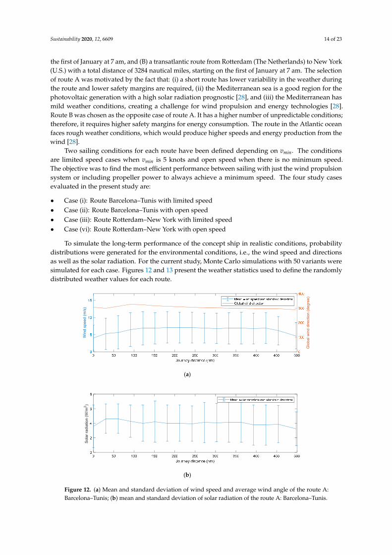
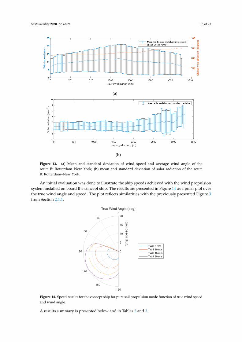
Two different routes were evaluated: (A) a short distance route in the Mediterranean Sea between the ports of Barcelona (Spain) and Tunis (Tunisia) with a total distance of 496 nautical miles, starting on the first of January at 7 am, and (B) a transatlantic route from Rotterdam (The Netherlands) to New York (U.S.) with a total distance of 3284 nautical miles, starting on the first of January at 7 am. The selection of route A was motivated by the fact that: (i) a short route has lower variability in the weather during the route and lower safety margins are required, (ii) the Mediterranean sea is a good region for the photovoltaic generation with a high solar radiation prognostic [28], and (iii) the Mediterranean has mild weather conditions, creating a challenge for wind propulsion and energy technologies [28]. Route B was chosen as the opposite case of route A. It has a higher number of unpredictable conditions; therefore, it requires higher safety margins for energy consumption. The route in the Atlantic ocean faces rough weather conditions, which would produce higher speeds and energy production from the wind [28].

Two sailing conditions for each route have been defined depending on 𝑣 . The conditions are limited speed cases when 𝑣 is 5 knots and open speed when there is no minimum speed. The objective was to find the most efficient performance between sailing with just the wind propulsion system or including propeller power to always achieve a minimum speed. The four study cases evaluated in the present study are:

• Case (i): Route Barcelona–Tunis with limited speed • Case (ii): Route Barcelona–Tunis with open speed • Case (iii): Route Rotterdam–New York with limited speed • Case (vi): Route Rotterdam–New York with open speed

To simulate the long-term performance of the concept ship in realistic conditions, probability distributions were generated for the environmental conditions, i.e., the wind speed and directions as well as the solar radiation. For the current study, Monte Carlo simulations with 50 variants were simulated for each case. Figures 12 and 13 present the weather statistics used to define the randomly distributed weather values for each route.

Figure 11. Propeller-hydro turbine 3D model from “OpenProp”.

3. Results

This section presents results from the numerical model, simulating the performance of the conceptship on routes under realistic weather conditions, intending to identify the optimal operation of theconcept ship under varying conditions

Two different routes were evaluated: (A) a short distance route in the Mediterranean Sea betweenthe ports of Barcelona (Spain) and Tunis (Tunisia) with a total distance of 496 nautical miles, starting on


the first of January at 7 am, and (B) a transatlantic route from Rotterdam (The Netherlands) to New York(U.S.) with a total distance of 3284 nautical miles, starting on the first of January at 7 am. The selectionof route A was motivated by the fact that: (i) a short route has lower variability in the weather duringthe route and lower safety margins are required, (ii) the Mediterranean sea is a good region for thephotovoltaic generation with a high solar radiation prognostic [28], and (iii) the Mediterranean hasmild weather conditions, creating a challenge for wind propulsion and energy technologies [28].Route B was chosen as the opposite case of route A. It has a higher number of unpredictable conditions;therefore, it requires higher safety margins for energy consumption. The route in the Atlantic oceanfaces rough weather conditions, which would produce higher speeds and energy production from thewind [28].

Two sailing conditions for each route have been defined depending on vmin. The conditionsare limited speed cases when vmin is 5 knots and open speed when there is no minimum speed.The objective was to find the most efficient performance between sailing with just the wind propulsionsystem or including propeller power to always achieve a minimum speed. The four study casesevaluated in the present study are:

• Case (i): Route Barcelona–Tunis with limited speed• Case (ii): Route Barcelona–Tunis with open speed• Case (iii): Route Rotterdam–New York with limited speed• Case (vi): Route Rotterdam–New York with open speed

To simulate the long-term performance of the concept ship in realistic conditions, probabilitydistributions were generated for the environmental conditions, i.e., the wind speed and directionsas well as the solar radiation. For the current study, Monte Carlo simulations with 50 variants weresimulated for each case. Figures 12 and 13 present the weather statistics used to define the randomlydistributed weather values for each route.


(a)

(b)

Figure 12. (a) Mean and standard deviation of wind speed and average wind angle of the route A: Barcelona–Tunis; (b) mean and standard deviation of solar radiation of the route A: Barcelona–Tunis.

(a)

Win

d sp

eed

(m/s

)

Glo

bal w

ind

dire

ctio

n (d

egre

e)

Sola

r rad

iatio

n (W

/m2 )

Win

d sp

eed

(m/s

)

Glo

bal w

ind

dire

ctio

n (d

egre

e)

Figure 12. (a) Mean and standard deviation of wind speed and average wind angle of the route A:Barcelona–Tunis; (b) mean and standard deviation of solar radiation of the route A: Barcelona–Tunis.



(a)

(b)

Figure 12. (a) Mean and standard deviation of wind speed and average wind angle of the route A: Barcelona–Tunis; (b) mean and standard deviation of solar radiation of the route A: Barcelona–Tunis.

(a)

Win

d sp

eed

(m/s

)

Glo

bal w

ind

dire

ctio

n (d

egre

e)

Sola

r rad

iatio

n (W

/m2 )

Win

d sp

eed

(m/s

)

Glo

bal w

ind

dire

ctio

n (d

egre

e)


(b)

Figure 13. (a) Mean and standard deviation of wind speed and average wind angle of the route B: Rotterdam–New York; (b) mean and standard deviation of solar radiation of the route B: Rotterdam–New York.

An initial evaluation was done to illustrate the ship speeds achieved with the wind propulsion system installed on board the concept ship. The results are presented in Figure 14 as a polar plot over the true wind angle and speed. The plot reflects similarities with the previously presented Figure 3 from Section 2.1.1.

Figure 14. Speed results for the concept ship for pure sail propulsion mode function of true wind speed and wind angle.

A results summary is presented below and in Tables 2 and 3.

Table 2. Summary of simulations results for route A (Barcelona–Tunis).

Simulation Restricted Speed Open Speed Average speed 5.36 knots 1.10 knots

Time 93 h 454 h Average power consumption 729 kW 258 kW

Average power generation 149 kW 153 kW Shore-based energy used 55702 kWh 58198 kWh

Sola

r rad

iatio

n (W

/m2 )

0

30

60

90

120

150

180

True Wind Angle (deg)

0

5

10

15

20

Ship

spe

ed (k

n)

TWS 5 m/sTWS 10 m/sTWS 15 m/sTWS 20 m/s

Figure 13. (a) Mean and standard deviation of wind speed and average wind angle of theroute B: Rotterdam–New York; (b) mean and standard deviation of solar radiation of the routeB: Rotterdam–New York.

An initial evaluation was done to illustrate the ship speeds achieved with the wind propulsionsystem installed on board the concept ship. The results are presented in Figure 14 as a polar plot overthe true wind angle and speed. The plot reflects similarities with the previously presented Figure 3from Section 2.1.1.


(b)

Figure 13. (a) Mean and standard deviation of wind speed and average wind angle of the route B:

Rotterdam–New York; (b) mean and standard deviation of solar radiation of the route B: Rotterdam–

New York.

An initial evaluation was done to illustrate the ship speeds achieved with the wind propulsion system

installed on board the concept ship. The results are presented in Figure 14 as a polar plot over the

true wind angle and speed. The plot reflects similarities with the previously presented Figure 3 from

Section 2.1.1.

Figure 14. Speed results for the concept ship for pure sail propulsion mode function of true wind

speed and wind angle.



Simulation Restricted Speed Open Speed

Average speed 5.36 knots 1.10 knots

Time 93 h 454 h

Average power consumption 729 kW 258 kW

Average power generation 149 kW 153 kW

Shore-based energy used 55702 kWh 58198 kWh

Figure 14. Speed results for the concept ship for pure sail propulsion mode function of true wind speedand wind angle.





Average speed 5.36 knots 1.10 knotsTime 93 h 454 h

Average power consumption 729 kW 258 kWAverage power generation 149 kW 153 kWShore-based energy used 55702 kWh 58198 kWh

Table 3. Summary of simulations results for route B (Rotterdam–New York).


Average speed 7.32 knots 4.29 knotsTime 448 h 765 h

Average power consumption 464 kW 305 kWAverage power generation 401 kW 395 kWShore-based energy used 84589 kWh 47189 kWh

Case (i): Route Barcelona–Tunis with limited speed

The first study case analyzes the Barcelona–Tunis route with a minimum speed of 5 knots.The voyage took (on average) 93 h, which gave an average speed of 5.3 knots. The average powerconsumption of the systems onboard was 729 kW, while the average power generation was 149 kW.At the end of the voyage, the energy balance showed that 55702 kWh were required in addition to theavailable renewable sources at sea. This is equivalent to 446 fully charged commercial marine batteriesof 125 kWh each and a weight of about 713 tons, considering that each battery weighs 1.6 tons [33].

Case (ii): Route Barcelona–Tunis with open speed

The second study case analyzes the Barcelona—Tunis route when the ship speed is not restricted.The voyage took (on average) 454 h, which gave an average speed of 1.10 knots. The average powerconsumption of the systems onboard was 258 kW, while the average power generation was 153 kW.At the end of the voyage, the energy balance showed that 58198 kWh were required in addition to theavailable renewable sources at sea. This is equivalent to 474 fully charged commercial marine batteriesof 125 kWh each and a weight of about 757 tons, considering that each battery weighs 1.6 tons [33].

Case (iii): Route Rotterdam–New York with limited speed

The third study case analyzes the Rotterdam–New York route for a minimum restricted speed to5 knots. The voyage took (on average) 448 h, which gave an average speed of 7.3 knots. The averagepower consumption of the systems onboard was 464 kW, while the average power generation was401 kW. At the end of the voyage, the energy balance showed that 84589 kWh were required in additionto the available renewable sources at sea. This is equivalent to 677 fully charged commercial marinebatteries of 125 kWh each and a weight of about 1082 tons, considering that each battery weighs1.6 tons [33].

Case (vi): Route Rotterdam–New York with open speed

The fourth study case analyzes the Rotterdam–New York route when the ship speed is notrestricted. The voyage took (on average) 765 h, which gave an average speed of 4.3 knots. The averagepower consumption of the systems onboard was 305 kW, while the average power generation was395 kW. At the end of the voyage, the energy balance showed that 47189 kWh were required inaddition to the available renewable sources at sea. This is equivalent to 378 fully charged commercialmarine batteries of 125 kWh each and a weight of about 604 tons, considering that each battery weighs1.6 tons [33].


In Figures 15 and 16, a comparison of the resulting ship speeds is presented for the route fromBarcelona to Tunis and from Rotterdam to New York. The plots represent in blue the study cases (i)and (iii) for limited speed and in red the study cases (ii) and (vi) with open speed mode. As the resultwas calculated for 50 different simulations, the plot presents the average speed together with the upperand lower speed levels.Sustainability 2020, 12, x FOR PEER REVIEW 18 of 25

Figure 15. Speed comparison route A (Barcelona–Tunis).

Figure 16. Speed comparison route B (Rotterdam–New York).

Results from route A, in Figure 15, show a considerable reduction in average ship speed (480%

reduction) when moving from limited speed (case i) to open speed (case ii). The average speed for

case (i) stays close to the limiting velocity; therefore, the wind propulsion is assisted with the

propeller in most of the trip.

The other route B, presented in Figure 16, shows similar average and speed variation curves for

both conditions (cases iii and iv). This result indicated that for both cases, the wind propulsion takes

a lead role in the ship propulsion.

As a comparison between routes A and B, it is shown that from a velocity point of view, the

restriction of the minimum speed of the ship is essential when considering the route A, but not as

relevant in route B. In route A, the energy produced from the wind is extremely reduced in some

parts of the route, and the thrust produced by the propeller eliminates those periods of low ship

speed. However, route B shows that additional thrust from the propeller does not have a relevant

influence to achieve the minimum speed.

Figures 17 and 18 present a comparison of the energy production for the different installed

technologies. Route A is presented in Figure 17 for study cases (i) and (ii), and route B in Figure 18

for cases (iii) and (iv). The plots present the mean energy production value for solar panels, wind

turbine, and hydro turbine. The plots show that for the same route, the average power production is

similar despite the minimum speed restriction. Minor differences can be noticed in hydro turbine

generation for route A, showing higher production levels for the open case (average case (ii) = 58.5

kW) than for limited cases (average case (i) = 36.0 kW). This is because the limited case does not

sacrifice speed (increasing drag coefficient) to produce energy if the minimum speed is not reached.

Comparing the routes A and B, it is noted that on route B, the energy produced by the hydro turbine

becomes predominant with respect to the other technologies presented above; this is caused by

stronger wind speeds and higher ship speed.





Results from route A, in Figure 15, show a considerable reduction in average ship speed (480%

reduction) when moving from limited speed (case i) to open speed (case ii). The average speed for

case (i) stays close to the limiting velocity; therefore, the wind propulsion is assisted with the

propeller in most of the trip.

The other route B, presented in Figure 16, shows similar average and speed variation curves for

both conditions (cases iii and iv). This result indicated that for both cases, the wind propulsion takes

a lead role in the ship propulsion.

As a comparison between routes A and B, it is shown that from a velocity point of view, the

restriction of the minimum speed of the ship is essential when considering the route A, but not as

relevant in route B. In route A, the energy produced from the wind is extremely reduced in some

parts of the route, and the thrust produced by the propeller eliminates those periods of low ship

speed. However, route B shows that additional thrust from the propeller does not have a relevant

influence to achieve the minimum speed.

Figures 17 and 18 present a comparison of the energy production for the different installed

technologies. Route A is presented in Figure 17 for study cases (i) and (ii), and route B in Figure 18

for cases (iii) and (iv). The plots present the mean energy production value for solar panels, wind

turbine, and hydro turbine. The plots show that for the same route, the average power production is

similar despite the minimum speed restriction. Minor differences can be noticed in hydro turbine

generation for route A, showing higher production levels for the open case (average case (ii) = 58.5

kW) than for limited cases (average case (i) = 36.0 kW). This is because the limited case does not

sacrifice speed (increasing drag coefficient) to produce energy if the minimum speed is not reached.

Comparing the routes A and B, it is noted that on route B, the energy produced by the hydro turbine

becomes predominant with respect to the other technologies presented above; this is caused by

stronger wind speeds and higher ship speed.


Results from route A, in Figure 15, show a considerable reduction in average ship speed(480% reduction) when moving from limited speed (case i) to open speed (case ii). The average speedfor case (i) stays close to the limiting velocity; therefore, the wind propulsion is assisted with thepropeller in most of the trip.

The other route B, presented in Figure 16, shows similar average and speed variation curves forboth conditions (cases iii and iv). This result indicated that for both cases, the wind propulsion takes alead role in the ship propulsion.

As a comparison between routes A and B, it is shown that from a velocity point of view,the restriction of the minimum speed of the ship is essential when considering the route A, but notas relevant in route B. In route A, the energy produced from the wind is extremely reduced in someparts of the route, and the thrust produced by the propeller eliminates those periods of low ship speed.However, route B shows that additional thrust from the propeller does not have a relevant influence toachieve the minimum speed.

Figures 17 and 18 present a comparison of the energy production for the different installedtechnologies. Route A is presented in Figure 17 for study cases (i) and (ii), and route B in Figure 18 forcases (iii) and (iv). The plots present the mean energy production value for solar panels, wind turbine,and hydro turbine. The plots show that for the same route, the average power production is similardespite the minimum speed restriction. Minor differences can be noticed in hydro turbine generationfor route A, showing higher production levels for the open case (average case (ii) = 58.5 kW) than for


limited cases (average case (i) = 36.0 kW). This is because the limited case does not sacrifice speed(increasing drag coefficient) to produce energy if the minimum speed is not reached. Comparingthe routes A and B, it is noted that on route B, the energy produced by the hydro turbine becomespredominant with respect to the other technologies presented above; this is caused by stronger windspeeds and higher ship speed.Sustainability 2020, 12, x FOR PEER REVIEW 19 of 25

Figure 17. Power production comparison route A (Barcelona–Tunis).

Figure 18. Power production comparison route B (Rotterdam–New York).

The energy consumption is presented in Figure 19 for route A and in Figure 20 for route B. The plots show the consumption of the Flettner rotors, the propeller, and the non-propulsive loads. For both routes, the propeller power demand naturally becomes zero for open speed cases (ii and iv). However, comparing the limited cases (i and iii), some differences can be noticed. Case (i) shows a mean energy demand of the propeller of 474 kW, while case (iii) has a mean value of 145 kW. These numbers highlight the influence of the propeller demand to the final ship consumption. While in case (i), propeller demand corresponds to 65% of the ship consumption, in case (iii) it corresponds to 31%. Small differences in the power demand from Flettner rotors are seen when comparing open and limited speed cases. Route B shows a slightly higher demand due to the more favorable wind conditions.

Figure 19. Power consumption comparison Route A (Barcelona–Tunis).

0 50 100 150 200 250 300 350 400 450 500Journey distance (nm)

0

50

100

150

200

250Average photovoltaic production case i)Average wind turbine production case i)Average hydro turbine production case i)

Average PV production case ii)Average wind turbine production case ii)Average Hydro-turbine production case ii)

0 500 1000 1500 2000 2500 3000 3500Journey distance (nm)

0

200

400

600

800 Average photovoltaic production case iii)Average wind turbine production case iii)Average hydro turbine production case iii)

Average PV production case iv)Average wind turbine production case iv)Average Hydro-turbine production case iv)


-600

-400

-200

0

200 Average non-propulsive consumption case i) and ii)Average Flettner rottor consumption case i)Average propeller consumption case i)

Average Flettner rottor consumption case ii)Average propeller consumption case ii)








0

50

100

150

200




0

200

400

600




-600

-400

-200

0




The energy consumption is presented in Figure 19 for route A and in Figure 20 for route B.The plots show the consumption of the Flettner rotors, the propeller, and the non-propulsive loads.For both routes, the propeller power demand naturally becomes zero for open speed cases (ii and iv).However, comparing the limited cases (i and iii), some differences can be noticed. Case (i) shows a meanenergy demand of the propeller of 474 kW, while case (iii) has a mean value of 145 kW. These numbershighlight the influence of the propeller demand to the final ship consumption. While in case (i),propeller demand corresponds to 65% of the ship consumption, in case (iii) it corresponds to 31%.Small differences in the power demand from Flettner rotors are seen when comparing open and limitedspeed cases. Route B shows a slightly higher demand due to the more favorable wind conditions.

Figures 21 and 22 present a comparison of the energy consumption and energy productiononboard for routes A and B, respectively. The presented values are the average and upper and lowervalue of the consumed and produced power. The limited speed cases (i and iii) are shown in blue,and the open speed cases (ii and iv) in red. Values above zero represent power generation, values belowzero power consumption.








0

50

100

150

200




0

200

400

600




-600

-400

-200

0



Figure 19. Power consumption comparison Route A (Barcelona–Tunis).Sustainability 2020, 12, x FOR PEER REVIEW 20 of 25

Figure 20. Power consumption comparison route B (Rotterdam–New York).

Figures 21 and 22 present a comparison of the energy consumption and energy production onboard for routes A and B, respectively. The presented values are the average and upper and lower value of the consumed and produced power. The limited speed cases (i and iii) are shown in blue, and the open speed cases (ii and iv) in red. Values above zero represent power generation, values below zero power consumption.

Figure 21. Power production—power consumption comparison route A (Barcelona–Tunis).

Figure 22. Power production—power consumption comparison route B (Rotterdam–New York).

From an energetical efficiency perspective, the results show that for route A, case (i) has an average demand of 729 kW, while the average production is 149 kW. For this case, the power required is about five times the energy produced by the renewable systems. This results in a challenging situation for the energy supply system. For the same route, case (ii), with similar average energy production (153 kW), has a smaller energy consumption of 258 kW. Even if the power balance stays in negative values, the power deficit is reduced.


-600

-400

-200

0

200 Average non-propulsive consumption case iii) and iv)Average Flettner rottor consumption case iii)Average propeller consumption case iii)

Average Flettner rottor consumption case iv)Average propeller consumption case iv)




Figures 21 and 22 present a comparison of the energy consumption and energy production

onboard for routes A and B, respectively. The presented values are the average and upper and lower

value of the consumed and produced power. The limited speed cases (i and iii) are shown in blue,

and the open speed cases (ii and iv) in red. Values above zero represent power generation, values

below zero power consumption.



From an energetical efficiency perspective, the results show that for route A, case (i) has an

average demand of 729 kW, while the average production is 149 kW. For this case, the power required

is about five times the energy produced by the renewable systems. This results in a challenging

situation for the energy supply system. For the same route, case (ii), with similar average energy

production (153 kW), has a smaller energy consumption of 258 kW. Even if the power balance stays

in negative values, the power deficit is reduced.




Figures 21 and 22 present a comparison of the energy consumption and energy production

onboard for routes A and B, respectively. The presented values are the average and upper and lower

value of the consumed and produced power. The limited speed cases (i and iii) are shown in blue,

and the open speed cases (ii and iv) in red. Values above zero represent power generation, values

below zero power consumption.



From an energetical efficiency perspective, the results show that for route A, case (i) has an

average demand of 729 kW, while the average production is 149 kW. For this case, the power required

is about five times the energy produced by the renewable systems. This results in a challenging

situation for the energy supply system. For the same route, case (ii), with similar average energy

production (153 kW), has a smaller energy consumption of 258 kW. Even if the power balance stays

in negative values, the power deficit is reduced.



From an energetical efficiency perspective, the results show that for route A, case (i) has an averagedemand of 729 kW, while the average production is 149 kW. For this case, the power required is aboutfive times the energy produced by the renewable systems. This results in a challenging situation for theenergy supply system. For the same route, case (ii), with similar average energy production (153 kW),has a smaller energy consumption of 258 kW. Even if the power balance stays in negative values,the power deficit is reduced.

The results on route B are similar for the two simulated cases (iii and iv). The average productionand demand are 401 kW and 464 kW for case (iii) and 395 kW and 305 kW for case (iv), respectively.

The results show that route A is energetically less appropriate than B for the ship concept.From a power balance point of view, the restriction of the minimum speed, i.e., cases (i) and (iii),is not beneficial.

Figures 23 and 24 present the average and upper and lower values for the energy accumulated inbatteries. Figure 23 shows results for route A (cases i and ii) and Figure 24 for route B (cases iii and iv).


The results on route B are similar for the two simulated cases (iii and iv). The average production

and demand are 401 kW and 464 kW for case (iii) and 395 kW and 305 kW for case (iv), respectively.

The results show that route A is energetically less appropriate than B for the ship concept. From

a power balance point of view, the restriction of the minimum speed, i.e., cases (i) and (iii), is not

beneficial.

Figures 23 and 24 present the average and upper and lower values for the energy accumulated

in batteries. Figure 23 shows results for route A (cases i and ii) and Figure 24 for route B (cases iii and

iv).

Figure 23. Energy storage comparison route A (Barcelona–Tunis).

Figure 24. Energy storage comparison route B (Rotterdam–New York).

For both routes, the non-restricted speed cases (ii and iv) show better performance. Comparing

the two routes, route B shows better performance with average energy stored on board of 538 kWh

for case (iii) and 992 kWh for case (iv). Route A fluctuates in a range of energy stored closer to zero.

Average stored energy is 7.07 kWh for case (i) and 22.4 kWh for case (ii).

Finally, the shore-based energy consumed is shown in Figures 25 and 26. Figure 25 shows results

for route A (cases i and ii) and Figure 26 for route B (cases iii and iv). The figure shows the total

energy required by the consumers that cannot be produced by the renewable systems beforehand.



The results on route B are similar for the two simulated cases (iii and iv). The average production

and demand are 401 kW and 464 kW for case (iii) and 395 kW and 305 kW for case (iv), respectively.

The results show that route A is energetically less appropriate than B for the ship concept. From

a power balance point of view, the restriction of the minimum speed, i.e., cases (i) and (iii), is not

beneficial.

Figures 23 and 24 present the average and upper and lower values for the energy accumulated

in batteries. Figure 23 shows results for route A (cases i and ii) and Figure 24 for route B (cases iii and

iv).



For both routes, the non-restricted speed cases (ii and iv) show better performance. Comparing

the two routes, route B shows better performance with average energy stored on board of 538 kWh

for case (iii) and 992 kWh for case (iv). Route A fluctuates in a range of energy stored closer to zero.

Average stored energy is 7.07 kWh for case (i) and 22.4 kWh for case (ii).

Finally, the shore-based energy consumed is shown in Figures 25 and 26. Figure 25 shows results

for route A (cases i and ii) and Figure 26 for route B (cases iii and iv). The figure shows the total

energy required by the consumers that cannot be produced by the renewable systems beforehand.


For both routes, the non-restricted speed cases (ii and iv) show better performance. Comparingthe two routes, route B shows better performance with average energy stored on board of 538 kWhfor case (iii) and 992 kWh for case (iv). Route A fluctuates in a range of energy stored closer to zero.Average stored energy is 7.07 kWh for case (i) and 22.4 kWh for case (ii).

Finally, the shore-based energy consumed is shown in Figures 25 and 26. Figure 25 shows resultsfor route A (cases i and ii) and Figure 26 for route B (cases iii and iv). The figure shows the total energyrequired by the consumers that cannot be produced by the renewable systems beforehand.

On route A, the ship requires (on average) 55,702 kWh of shore-based energy in case (i) and58,198 kWh in case (ii). Similar final results show that the increment in time for the route (ii) does notprovide energetical benefits. On route B, the ship requires 84589 kWh in case (iii) and 47189 kWh incase (iv), on average. On this route, the energy efficiency is improved for an extended time at sea, i.e.,


for the case without a minimum speed limit. Considering the amount of shore-based energy used permile, case (i) requires 112 kWh/nautical mile, case (ii) 117 kWh/nautical mile, case (iii) 25.8 kWh/nauticalmile, and case (iv) 14.4 kWh/nautical mile. These results show that the efficiency and viability of sailingpurely with renewable energy are considerably higher on route B.Sustainability 2020, 12, x FOR PEER REVIEW 22 of 25

Figure 25. Shore-based energy consumption comparison route A (Barcelona–Tunis).

Figure 26. Shore-based energy consumption comparison route B (Rotterdam–New York).

On route A, the ship requires (on average) 55702 kWh of shore-based energy in case (i) and 58198

kWh in case (ii). Similar final results show that the increment in time for the route (ii) does not provide

energetical benefits. On route B, the ship requires 84589 kWh in case (iii) and 47189 kWh in case (iv),

on average. On this route, the energy efficiency is improved for an extended time at sea, i.e., for the

case without a minimum speed limit. Considering the amount of shore-based energy used per mile,

case (i) requires 112 kWh/nautical mile, case (ii) 117 kWh/nautical mile, case (iii) 25.8 kWh/nautical

mile, and case (iv) 14.4 kWh/nautical mile. These results show that the efficiency and viability of

sailing purely with renewable energy are considerably higher on route B.

4. Discussion and Conclusions

This study presents a novel method and model of a concept ship to evaluate the possibilities that

renewable technologies can offer to the marine shipping industry. The numerical model used was

developed to simulate the performance of a fossil-free operated cargo ship in realistic weather

conditions. The presented methodology integrated real route conditions with the ship performance

model ShipCLEAN [15,17], which simulated the ship performance using Flettner rotors together with

renewable electric generators and an energy storage system to estimate the available energy. This

integration made it possible to evaluate ship journey times, energy consumption, and energy

production for different routes, ship types, sailing conditions, and renewable energy system

configurations. Four study cases were compared, two on a Mediterranean route between Barcelona

and Tunis and two on a transoceanic route between Rotterdam and New York.

The route Barcelona—Tunis is the most challenging for a fossil-free cargo ship. The route is

shorter, with favorable solar radiation but low wind speeds. The results show low ship speeds,

resulting in a long time at sea (case ii) or in an increase of energy demand from the propeller to

provide the additional thrust that requires much more energy than produced by renewable

systems.





On route A, the ship requires (on average) 55702 kWh of shore-based energy in case (i) and 58198

kWh in case (ii). Similar final results show that the increment in time for the route (ii) does not provide

energetical benefits. On route B, the ship requires 84589 kWh in case (iii) and 47189 kWh in case (iv),

on average. On this route, the energy efficiency is improved for an extended time at sea, i.e., for the

case without a minimum speed limit. Considering the amount of shore-based energy used per mile,

case (i) requires 112 kWh/nautical mile, case (ii) 117 kWh/nautical mile, case (iii) 25.8 kWh/nautical

mile, and case (iv) 14.4 kWh/nautical mile. These results show that the efficiency and viability of

sailing purely with renewable energy are considerably higher on route B.


This study presents a novel method and model of a concept ship to evaluate the possibilities that

renewable technologies can offer to the marine shipping industry. The numerical model used was

developed to simulate the performance of a fossil-free operated cargo ship in realistic weather

conditions. The presented methodology integrated real route conditions with the ship performance

model ShipCLEAN [15,17], which simulated the ship performance using Flettner rotors together with

renewable electric generators and an energy storage system to estimate the available energy. This

integration made it possible to evaluate ship journey times, energy consumption, and energy

production for different routes, ship types, sailing conditions, and renewable energy system

configurations. Four study cases were compared, two on a Mediterranean route between Barcelona

and Tunis and two on a transoceanic route between Rotterdam and New York.

The route Barcelona—Tunis is the most challenging for a fossil-free cargo ship. The route is

shorter, with favorable solar radiation but low wind speeds. The results show low ship speeds,

resulting in a long time at sea (case ii) or in an increase of energy demand from the propeller to

provide the additional thrust that requires much more energy than produced by renewable

systems.



This study presents a novel method and model of a concept ship to evaluate the possibilitiesthat renewable technologies can offer to the marine shipping industry. The numerical modelused was developed to simulate the performance of a fossil-free operated cargo ship in realisticweather conditions. The presented methodology integrated real route conditions with the shipperformance model ShipCLEAN [15,17], which simulated the ship performance using Flettner rotorstogether with renewable electric generators and an energy storage system to estimate the availableenergy. This integration made it possible to evaluate ship journey times, energy consumption,and energy production for different routes, ship types, sailing conditions, and renewable energy systemconfigurations. Four study cases were compared, two on a Mediterranean route between Barcelonaand Tunis and two on a transoceanic route between Rotterdam and New York.

• The route Barcelona—Tunis is the most challenging for a fossil-free cargo ship. The route is shorter,with favorable solar radiation but low wind speeds. The results show low ship speeds, resultingin a long time at sea (case ii) or in an increase of energy demand from the propeller to provide theadditional thrust that requires much more energy than produced by renewable systems.

• Route Rotterdam—New York, has a longer distance, but the ship shows better speed performanceand energy results in both study cases (iii and iv). The favorable wind conditions along mostof the route provide high enough speeds to avoid the use of the propeller and to produce high


energy levels with the hydro turbine. As a result, the energy balance is improved requiring lessstored energy.

• In all four study cases, it has been shown that it is not possible to achieve current freight marketspeeds with purely renewable-powered ships. Marine shipping speeds must be readapted.Further, the sailing region and routing become important parameters for the speed selection.

• When considering the dual-mode propeller and wind turbine technology, it is essential toevaluate the balance between speed and energy production. The technology can produce highenergy production, but always with a considerably high sacrifice in ship speed due to the dragforce created.

• In all studied cases, energy stored in the batteries onboard before the start of the trip is required,to compensate the additional energy consumption not produced by the renewable systems(shore-based energy).

A fossil-free operated cargo ship was introduced and simulated effectively, the advantages andchallenges of the renewable systems onboard were highlighted, and the multiple study cases definedthose sailing conditions where a vessel with similar characteristics would provide high efficiency.The impact of the present study for future research is to demonstrate that with the existing technologies,there is the possibility to operate a fossil-free vessel. Future research from the conclusions is requiredto investigate how particular ship designs, renewable systems, and sailing conditions can influence theefficiency of the journey to be able to optimize a renewable power vessel for its unique operation.

Author Contributions: Conceptualization: E.J., F.T., and J.W.R.; methodology: E.J. and F.T.; software: E.J. andF.T.; validation: E.J. and F.T.; formal analysis: E.J. and F.T.; investigation: E.J. and F.T.; resources: E.J. and F.T.;data curation: E.J. and F.T.; writing—original draft preparation: E.J.; writing—review and editing: F.T. and J.W.R.;visualization: E.J. and F.T.; supervision: F.T. and J.W.R.; project administration: F.T. and J.W.R.; funding acquisition:J.W.R. All authors have read and agreed to the published version of the manuscript.

Funding: This work was supported by The Swedish Energy Agency (grant number P44454-1) for funding theproject “ShipCLEAN—Energy efficient marine transport through optimization of coupled transportation logisticsand energy systems analyses”.

Conflicts of Interest: The authors declare no conflict of interest.

References

1. Harrould-Kolieb, E. Shipping Impacts on Climate: A Source with Solution. Available online: https://usa.oceana.org/sites/default/files/reports/Oceana_Shipping_Report1.pdf (accessed on 2 February 2019).

2. Margaritou, M.D.; Tzannatos, E. A multi-criteria optimization approach for solar energy and wind powertechnologies in shipping. FME Trans. 2018, 46, 374–380. [CrossRef]

3. Atkinson, G.; Nguyen, H.; Binns, J. Considerations regarding the use of rigid sails on modern powered ships.Cogent Eng. 2018, 5, 1–20. [CrossRef]

4. Ouchi, K.; Uzawa, K.; Kanai, A. Huge Hard Wing Sails for the Propulsor of Next Generation Sailing Vessel.In Proceedings of the Second International Symposium on Marine Propulsors, Hamburg, Germany, 15–17 June 2011.

5. Talluri, L.; Nalianda, D.K.; Giuliani, E. Techno economic and environmental assessment of Flettner rotors formarine propulsion. Ocean Eng. 2018, 154, 1–15. [CrossRef]

6. Leloup, R.; Roncin, K.; Behrel, M.; Bles, G.; Leroux, J.B.; Jochum, C.; Parlier, Y. A continuous and analyticalmodeling for kites as auxiliary propulsion devoted to merchant ships, including fuel saving estimation.Renew. Energy 2016, 86, 483–496. [CrossRef]

7. Traut, M.; Gilbert, P.; Walsh, C.; Bows, A.; Filippone, A.; Stansby, P.; Wood, R. Propulsive power contributionof a kite and a Flettner rotor on selected shipping routes. Appl. Energy 2013, 113, 362–372. [CrossRef]

8. Kim, T.K.; Yaakob, O. Adaptation of Wind Power for Ship Essential Service System Onboard. J. Transp.Syst. Eng. 2016, 1, 8–19.

9. Clarson, O.; Nilsson, P. Wind Turbines on Ships. Available online: http://publications.lib.chalmers.se/

publication/217076 (accessed on 13 August 2020).10. Lan, H.; Wen, S.; Hong, Y.Y.; Yu, D.C.; Zhang, L. Optimal sizing of hybrid PV/diesel/battery in ship power

system. Appl. Energy 2015, 158, 26–34. [CrossRef]

https://usa.oceana.org/sites/default/files/reports/Oceana_Shipping_Report1.pdf

https://usa.oceana.org/sites/default/files/reports/Oceana_Shipping_Report1.pdf

http://dx.doi.org/10.5937/fmet1803374M

http://dx.doi.org/10.1080/23311916.2018.1543564

http://dx.doi.org/10.1016/j.oceaneng.2018.02.020

http://dx.doi.org/10.1016/j.renene.2015.08.036

http://dx.doi.org/10.1016/j.apenergy.2013.07.026

http://publications.lib.chalmers.se/publication/217076

http://publications.lib.chalmers.se/publication/217076

http://dx.doi.org/10.1016/j.apenergy.2015.08.031


11. Liu, P.; Bose, N.; Chen, K.; Xu, Y. Development and optimization of dual-mode propellers for renewableenergy. Renew. Energy 2018, 119, 566–576. [CrossRef]

12. YUTUC, W. Use of hydro generator on a tanker ship: A computer-generated simulation study. Lect. NotesComput. Sci. (Incl. Subser. Lect. Notes Artif. Intell. Lect. Notes Bioinform.) 2013, 7972, 207–219.

13. Bøckmann, E. Wave Propulsion of Ships. Ph.D. Thesis, Norwegian University of Science and Technology,Trodheim, Norway, 2015.

14. Julià, E. Concept Development of a Fossil Free Operated Cargo Ship. Master’s Thesis, Chalmers Universityof Technology, Gothenburg, Sweden, 2019.

15. Tillig, F.; Ringsberg, J. Design, operation and analysis of wind-assisted cargo ships. Ocean Eng. 2020, 211,107603. [CrossRef]

16. Lu, R.; Ringsberg, J.W. Ship energy performance study of three windassisted ship propulsion technologiesincluding a parametric study of the Flettner rotor technology. Ships Offshore Struct. 2020, 15, 249–258. [CrossRef]

17. Tillig, F.; Ringsberg, J.W. A 4 DOF simulation model developed for fuel consumption prediction of ships atsea. Ships Offshore Struct. 2018, 14, 112–120. [CrossRef]

18. Epps, B. On the rotor lifting line wake model. J. Sh. Prod. Des. 2017, 33, 31–45. [CrossRef]19. Swoboda, R. Shaft Generators: Propelling Vessels toward Leaner, Greener Power Generation. Available

online: https://www.wartsila.com/twentyfour7/in-detail/shaft-generators-propelling-vessels-toward-leaner-greener-power-generation (accessed on 15 October 2019).

20. Möllerström, E.; Ottermo, F.; Tillig, F.; Ringsberg, J.W.; Psaraftis, H.N.; Zis, T. ShipCLEAN–An integrated model fortransport efficiency, economics and CO2 emissions in shipping. In Proceedings of the 2nd International Conferenceon Modelling and Optimisation of Ship Energy Systems, Glasgow, UK, 8–10 May 2019.

21. Goude, A.; Eriksson, S.; Hylander, J.; Bernhoff, H. Turbulence influence on wind energy extraction for amedium size vertical axis wind turbine. Wind Energy 2016, 19, 1963–1973.

22. Yu, D.; Wen, S.; Dai, J.; Lan, H.; Bai, Y.; Hong, Y. Optimal Tilt Angle of Photovoltaic Arrays and EconomicAllocation of Energy Storage System on Large Oil Tanker Ship. Energies 2015, 8, 11515–11530.

23. Vieira Da Rosa, A. Fundamentals of Renewable Energy Processes, 3rd ed.; Elsevier: Oxford, UK, 2005; pp. 455–493.24. Ekici, S.; Kopru, M.A. Investigation of PV system cable losses. Int. J. Renew. Energy Res. 2017, 7, 807–815.25. Setiawan, F.; Dewi, T.; Yusi, S. Sea Salt Deposition Effect on Output and Efficiency Losses of the Photovoltaic

System; a case study in Palembang, Indonesia. J. Phys. Conf. Ser. 2019, 1167, 1–11. [CrossRef]26. Shaft Generators for Low-Speed Main Engines. Available online: https://marine.mandieselturbo.com/docs/

librariesprovider6/technical-papers/shaft-generators-for-mc-and-me-engines.pdf?sfvrsn=22 (accessed on23 November 2019).

27. Fetcenko, M.A.; Ovshinsky, S.R.; Reichman, B.; Young, K.; Fierro, C.; Koch, J.; Ouchi, T. Recent advances inNiMH battery technology. J. Power Sources 2007, 165, 544–551. [CrossRef]

28. Miglietta, M.M.; Huld, T.; Monforti-Ferrario, F. Local Complementarity of Wind and Solar Energy Resourcesover Europe: An Assessment Study from a Meteorological Perspective. J. Appl. Meteorol. Climatol. 2017, 56,217–234. [CrossRef]

29. Peral Pérez, I. Diseño de la Instalación Eléctrica de un Petrolero Para Transporte de Crudo. Master’s Thesis,Polytechnic University of Catalonia, Barcelona, Spain, 2013.

30. Verkinderen, E.; Boulent, I. A simplified dynamic model for mast design of H-Darrieus vertical axis windturbines (VAWTs). Eng. Struct. 2015, 100, 564–576. [CrossRef]

31. Tao, Y. Selection of a 50 kW Small Wind Turbine for Calgary. Master’s Thesis, University of Calgary, Calgary,AB, Canada, 2018.

32. Premier Solar Module Mounting Structures. Available online: https://www.premierispat.com/uploads/products/489960667brochure.pdf (accessed on 30 June 2020).

33. Corvus Energy. Available online: https://corvusenergy.com (accessed on 20 January 2020).

© 2020 by the authors. Licensee MDPI, Basel, Switzerland. This article is an open accessarticle distributed under the terms and conditions of the Creative Commons Attribution(CC BY) license (http://creativecommons.org/licenses/by/4.0/).

http://dx.doi.org/10.1016/j.renene.2017.12.041

http://dx.doi.org/10.1016/j.oceaneng.2020.107603

http://dx.doi.org/10.1080/17445302.2019.1612544

http://dx.doi.org/10.1080/17445302.2018.1559912

http://dx.doi.org/10.5957/JSPD.33.1.150035

https://www.wartsila.com/twentyfour7/in-detail/shaft-generators-propelling-vessels-toward-leaner-greener-power-generation

https://www.wartsila.com/twentyfour7/in-detail/shaft-generators-propelling-vessels-toward-leaner-greener-power-generation

http://dx.doi.org/10.1088/1742-6596/1167/1/012028

https://marine.mandieselturbo.com/docs/librariesprovider6/technical-papers/shaft-generators-for-mc-and-me-engines.pdf?sfvrsn=22

https://marine.mandieselturbo.com/docs/librariesprovider6/technical-papers/shaft-generators-for-mc-and-me-engines.pdf?sfvrsn=22

http://dx.doi.org/10.1016/j.jpowsour.2006.10.036

http://dx.doi.org/10.1175/JAMC-D-16-0031.1

http://dx.doi.org/10.1016/j.engstruct.2015.06.041

https://www.premierispat.com/uploads/products/489960667brochure.pdf

https://www.premierispat.com/uploads/products/489960667brochure.pdf

https://corvusenergy.com

http://creativecommons.org/

http://creativecommons.org/licenses/by/4.0/.

Concept Design and Performance Evaluation of a Fossil-Free ...

Documents

Transcript of Concept Design and Performance Evaluation of a Fossil-Free ...