Finance and Economics Discussion SeriesDivisions of Research & Statistics and Monetary Affairs

Federal Reserve Board, Washington, D.C.

Collateral Runs

Sebastian Infante and Alexandros P. Vardoulakis

2018-022

Please cite this paper as:Infante, Sebastian, and Alexandros P. Vardoulakis (2018). “Collateral Runs,” Finance andEconomics Discussion Series 2018-022. Washington: Board of Governors of the FederalReserve System, https://doi.org/10.17016/FEDS.2018.022.

NOTE: Staff working papers in the Finance and Economics Discussion Series (FEDS) are preliminarymaterials circulated to stimulate discussion and critical comment. The analysis and conclusions set forthare those of the authors and do not indicate concurrence by other members of the research staff or theBoard of Governors. References in publications to the Finance and Economics Discussion Series (other thanacknowledgement) should be cleared with the author(s) to protect the tentative character of these papers.

Collateral Runs∗

Sebastian Infante Alexandros P. Vardoulakis

Federal Reserve Board

March 28, 2018

Abstract: This paper models an unexplored source of liquidity risk faced by large broker-

dealers: collateral runs. By setting different contracting terms on repurchase agreements

with cash borrowers and lenders, dealers can source funds for their own activities. Cash

borrowers internalize the risk of losing their collateral in case their dealer defaults, prompting

them to withdraw it. This incentive creates strategic complementarities for counterparties

to withdraw their collateral, reducing a dealer’s liquidity position and compromising her

solvency. Collateral runs are markedly different than traditional wholesale funding runs

because they are triggered by a contraction in dealers’ assets, rather than their liabilities.

JEL classification: G23, G33, G01, C72

Keywords : runs, repo, rehypothecation, dealer, liquidity, default, collateral

∗We are grateful to brown bag participants at the Federal Reserve Board and Duke Fuqua School ofBusiness for fruitful comments and suggestions. All remaining errors are ours. The views of this paper aresolely the responsibility of the authors and should not be interpreted as reflecting the views of the Board ofGovernors of the Federal Reserve System or of any other person associated with the Federal Reserve System.Please send comments to sebastian.infantebilbao@frb.gov or alexandros.vardoulakis@frb.gov.

1

1 Introduction

This paper presents a theoretical model to characterize a relatively unexplored risk that can

affect large broker-dealers: a run from their collateral providers (cash borrowers). Broker-

dealers are unique because they transform liquidity on both sides of their balance sheet.

On the liabilities side, they borrow funds, typically short-term, from cash lenders, using

financial securities as collateral. On the asset side, they extend credit, also typically short-

term, against similar collateral provided by cash borrowers. In the context of the 2007–09

financial crisis, a large literature has noted that financial institutions faced run risk from their

wholesale funding lenders (see, for example, Gorton and Metrick, 2012; Krihnamurthy, Nagel,

and Orlov, 2014; and Copeland, Martin, and Walker, 2014). In this paper, we highlight an

alternative channel, which operates on the asset side of the balance sheet. Unlike traditional

wholesale funding runs, where dealers risk an abrupt withdrawal of funds from cash lenders,

in collateral runs, dealers risk an abrupt withdrawal of collateral from collateral providers.

The main set-up of the model considers a dealer providing short-term secured financing,

interpreted as repurchase agreements (repos), to a large number of counterparties, called

hedge funds. Hedge funds borrow from the dealer because they want to take leveraged

positions in the asset that they pledge as collateral. The dealer is able to extend said

financing by re-using the collateral she receives to issue secured debt to cash lenders, called

money market funds, a process known as rehypothecation.1 The dealer’s market power

allows her to set favorable contracting terms on both secured financing transactions. In

particular, she has incentives to distribute only a fraction of the cash she raises from money

funds and use the difference to finance higher-yielding risky assets, which are illiquid. In

case the dealer defaults, money funds have immediate access to the collateral and can sell it

to make their claims whole, essentially insulating them from the dealer. In contrast, hedge

funds risk losing their collateral altogether, which is more valuable than the initial loan they

received. This arrangement effectively gives hedge funds an unsecured claim on the dealer

and creates incentives for them to withdraw their collateral early, rather than roll over their

repos.

1We assume that hedge funds cannot contact money market funds directly—that is, their only source ofsecured financing for the hedge fund is through the dealer. This assumption captures the idea that manyhedge funds are small and relatively opaque firms, which wholesale cash lenders will not (or cannot) interactwith directly. Note that we will use the terms re-use and rehypothecation interchangeably.

2

The incentive to withdraw the collateral creates strategic complementarities amongst

hedge funds’ actions because each hedge fund’s optimal action and payoff can depend on what

other hedge funds do. For example, if all other hedge funds roll over their repo positions,

then the dealer does not need to liquidate any of her illiquid assets, making it optimal for an

individual hedge fund to roll over as well. On the contrary, if all other hedge funds withdraw

their collateral, then the dealer may need to sell off all of her illiquid assets, making it

optimal for an individual hedge fund to withdraw their collateral. Hence, an individual

hedge fund’s payoff not only depends on the dealer’s solvency, but also on its beliefs about

the actions/beliefs of other hedge funds. There are also extreme cases in which a hedge

fund’s actions are independent of other hedge funds’ actions. For example, if the value

of the dealer’s illiquid assets are low enough, she will be insolvent, making it individually

optimal for a hedge fund to withdraw, independent of others’ actions. Conversely, if the

value of the dealer’s illiquid assets are high enough, she will have ample liquidity to repay

all counterparties, making it individually optimal for a hedge fund to roll over, independent

of others’ actions. We establish when such extreme cases arise and show the existence of

intermediate situations where the dealer is solvent but illiquid.

The situation of a solvent but illiquid dealer introduces a coordination problem among

hedge funds akin to coordination problems in currency attacks (Morris and Shin, 1998), risky

debt rollover and bank runs (Diamond and Dybvig, 1983; Morris and Shin, 2004; Rochet

and Vives, 2004; Goldstein and Pauzner, 2005; He and Xiong, 2012; Vives, 2014), credit

market freezes (Bebchuk and Goldstein, 2011), and investment funds (Chen, Goldstein, and

Jiang, 2010; Liu and Mello, 2011). As is generally the case in coordination games, multiple

equilibria may exist. In order to find a unique equilibrium and characterize the optimal

contracting terms that give rise to it, we model an incomplete information game (global

game), similar to Goldstein and Pauzner (2005), where hedge funds receive noisy signals

about the (fundamental) expected value of the dealer’s risky investment. Moreover, we

extend their framework by introducing a stochastic liquidation value for the risky investment,

which is proportional to its fundamental value (see also Kashyap et al., 2017, for such an

extension under a different source of stochastic uncertainty). On the one hand, a stochastic

liquidation value enables the endogenous derivation of the regions for fundamentals where

individual actions are independent of other funds’ actions.2 On the other hand, it adds

2These are known as upper and lower dominance regions and are essential for the existence of equilibrium.

3

additional complexity in the proof of the uniqueness of a run equilibrium. Thus, we extend

the proof in Goldstein-Pauzner to account for stochastic liquidation values.

Establishing a unique threshold equilibrium shows the existence of a panic-based run.

That is, even though fundamentals may not be bad enough to make the dealer insolvent,

hedge funds incentives to withdraw early can render the dealer illiquid. This mechanism

highlights a novel fragility in the short-term funding intermediation process: a coordination

failure amongst collateral providers. The main contribution of this paper is to formalize

counterparties’ strategic complementarities and to characterize how these complementarities

can lead to a dealer’s endogenous default due to fundamental- or panic-based collateral runs.

Moreover, we underscore the relationship between the amount of overcollateralization (i.e.,

repo haircuts), the repo rate, and the dealer’s stability.

Note that the underlying collateral pledged by hedge funds and re-used by the dealer can

differ significantly from the risky asset purchased by the dealer. Specifically, the underlying

collateral can be extremely safe, yet there can still can be a collateral run. The risk that

collateral providers face does not come from their own assets, but rather from the dealer’s use

of the excess funds she raises with them. Duffie (2013) recognizes that an important source

of liquidity for dealers stems from their levered counterparties’ assets pledged as collateral,

while Infante (2017) characterizes the optimal contracting terms that lead to a liquidity

windfall whenever a dealer intermediates repos from one cash lender to one cash borrower.

However, neither of these two papers examines how such liquidity windfalls can introduce

dealer illiquidity, coordination failures, and run risk.3

An important motivating example of our paper is the demise of Bear Stearns in March

2008. Anecdotally, in the days leading up to its collapse, the firm suffered a large outflow of

counterparties that not only pulled their cash but also their collateral from the firm. Using

the Federal Reserve Bank of New York’s (FRBNY) weekly survey of primary dealers (FR

The upper dominance region is defined as the area where fundamentals are so good that an individual hedgefund rolls over its repo even if all other funds choose to withdraw. Allowing the liquidation value of riskyinvestment to move with the realization of fundamentals facilitates the endogenous derivation of the upperdominance region. The lower dominance region is defined as the area where fundamentals are so bad thatan individual hedge fund withdraws its collateral even if all other funds choose to roll over. The fact thatthe dealer defaults in some state of the world is sufficient to guarantee the existence of the lower dominanceregion.

3Infante (2017) provides a brief discussion of the relevant institutional details surrounding the re-use ofcollateral in the United States. In particular, in the context of repo, there are no limits to rehypothecation.

4

2004), we can estimate a lower bound on the total amount of cash that Bear Stearns accessed

through rehypothecation. Specifically, the FR 2004 asks primary dealers to report the total

amount of secured financing extended (Securities In), the total amount of secured financing

received (Securities Out), and their outright positions for different asset classes. Importantly,

the survey asks dealers to report the total amount of funds received and distributed though

secured financing transactions, not the value of the collateral posted. Therefore, these data

can be used to estimate the amount of liquidity obtained through contracting differences.

Figure 1 shows Bear Stearns’ repo activity in the months leading up to its default. The

difference between Securities Out (green line) and Securities In plus the firm’s net position

(red line) is an estimate of a lower bound on the total amount of funds raised through

differences in haircuts.4 From the figure, it can be appreciated that 1) the lion’s share of

securities the firm could post in secured financing transactions came from collateral sourced

from their counterparties (blue line), and 2) before the sharp drop in activity, the estimated

cash stemming from different contracting terms reached $50 billion, approximately a third of

the firm’s entire repo book. A withdrawal of collateral effectively eliminated this additional

liquidity windfall. To put this magnitude into perspective, Figure 2 plots the estimated cash

windfall as a fraction of the total repo book for both Bear Stearns and the average fraction

for the remaining primary dealers. These estimates suggest that, relative to its peers, Bear

Stearns relied heavily on differences in contracting terms as a source of liquidity.

Our paper is also related to the theoretical literature that characterizes optimal contract-

ing terms and instability in collateralized short-term funding markets. Fostel and Geanako-

plos (2015) derive the optimal haircuts on secured debt. Geanakoplos (2003), Fostel and

Geanakoplos (2008)—including a series of subsequent papers—and Simsek (2013) study the

interlinkages between asset prices, haircuts and leverage over the cycle as well as the im-

plications for investment and financial stability. Martin et al. (2014) detail the contracting

terms that lead to traditional cash-driven repo runs.5 We differ from these papers because

4The lower bound depends on an important restriction that securities dealers face: the box constraint.Broadly speaking, the box constraint is a physical restriction that forces dealers to have access to securities,either by owning them outright or by borrowing them, in order to deliver to a counterparty. Huh and Infante(2017) characterize how this constraint is important for bond market intermediation and how to interpretthe data in the FR 2004. Details on the lower-bound calculation and some potential caveats are in subsectionC of the Appendix.

5Many other theoretical papers have studied spirals and freezes in short-term funding markets. Someexamples are Brunnermeier and Pedersen (2009), Acharya et al. (2011), Diamond and Rajan (2011), and

5

we examine a distinct source of instability in repo intermediation. In the aforementioned

papers, the instability stems from the liability side of the balance sheet; cash lenders may be

less willing to provide funding and either require higher margins, leading to borrower delever-

aging, or withdraw their funding altogether in a coordinated run episode. In contrast, the

instability we study in this paper is borne from the asset side of an intermediaries balance

sheet; borrowers may collectively withdraw their collateral even if cash-lenders’ claims are

safe with stable haircuts (and not procyclical) and have no incentive to run.6

The rest of the paper is structured as follows. Section 2 presents the model setup, detailing

the economic environment, the main actors, and their incentives. Section 3 characterizes the

coordination problem hedge funds face, their threshold strategies, and the regions where

fundamental- or panic-based runs can materialize. Section 4 presents the problem the dealer

faces given hedge funds’ threshold strategies, characterizes the optimal contracting terms,

and numerically shows how the equilibria can change with fundamentals. Finally, section 5

gives some concluding remarks. All proofs are relegated to the Appendix.

2 Model Setup

The model consists of three periods t ∈ 0, 1, 2 and is populated by three types of agents; a

broker-dealer (D), a continuum of hedge funds (H), and a continuum of money market funds

(M). The money fund sector is assumed to be competitive. The dealer is (potentially) risk

averse, with a payoff function u that satisfies u(0) = 0, hedge funds are risk-neutral, and

money market funds are “very” risk averse.7 All agents discount the future the same way.

The timeline is presented in Figure 3.

Hedge funds would like to borrow to invest in a (safe) asset T , which is in perfect elastic

supply and is worth 1 in every period. Abusing notation, T will also denote the amount of

the asset purchased. Each hedge fund borrows money from the dealer at t = 0 (a reverse

repo from the dealer’s point of view), purchases the asset, and pledges it as collateral.

Ahnert (2016). As mentioned, we differ from this literature because we mute the rollover risk of cash-lenderspositions.

6In the context of micro finance, Bond and Rai (2009) also study instabilities arising from coordinateddefaults impacting the asset side of a lender’s balance sheet.

7The assumption that the dealer’s payoff function has u(0) = 0 is merely for simplicity. “Very” risk aversemoney funds will be useful to focus on the collateral channel, rather than the traditional repo-run channel.

6

Securities Out

Securities In + Net Position

Securities In

0

50

100

150

2006 2007 2008

Bear Stearns All SecuritiesBillions of dollars

Weekly

Source: FR 2004C and FR2004A

March 12th 2008

Figure 1: Securities Position of a Bear StearnsFigure shows the total amount of secured financing extended (securities in—blue line),the total amount of secured financing received (securities out—green line), and the sumbetween securities in and the dealers’ net-securities position (red line). The differencebetween the green line and the red line proxies for the additional liquidity the dealerreaps from re-using collateral. Source: FR 2004.

7

Bear Stearns

All Primary Dealers Excluding Bear Stearns

−60

−40

−20

0

20

40

60

2006 2007 2008

Estimated Cash Windfall as a Fraction of Total Repo BookPercent

Weekly

Note: Fraction calculated by (Securities Out − (Securities In + Net Position))/ Securities Out

Source: FR 2004C and FR2004A

March 12th 2008

Figure 2: Liquidity from Rehypothecation as a Fraction of Total Repo ActivityFigure shows the lower-bound estimate of the liquidity sourced through dealers’ repoactivity (securities out minus securities in and net position) as a fraction of their totalsecured financing (securities out) for both Bear Stearns and average fraction for the restof the primary dealer community. Source: FR 2004.

8

t = 0

D offers rev repo to HD offers repo to M

H purchases repo collateralD purchases risky asset cash surplus

t = 1

D offers new reposH decides to withdraw or roll overD may sell fraction risky position

t = 2

Asset uncertainty realizedCash flows distributed

Contracts settled

Figure 3: Model Timeline

Simultaneously, the dealer enters into a repo contract with money market funds, whereby

she rehypothecates the pledged collateral. We assume that the “number” of reverse repo

contracts is equal to the “number” of repo contracts, or in other words, an individual money

market fund is anonymously funding an individual hedge fund through dealer intermediation.

Repo contracts are short term, i.e., they mature after one period, and can be rolled over at

t = 1 as we describe further below.

Apart from intermediating between hedge funds and money funds, the dealer can also

invest at t = 0 in a risky asset R which pays off RU with probability θ and RD otherwise

in t = 2 per unit purchased, where RU > 1 > RD ≥ 0. The state of the world θ is realized

at t = 1 and follows a uniform distribution θ ∼ U [0, 1]. The risky asset has price of 1, is in

perfect elastic supply, and its expected value, conditional on θ, is denoted by Eθ(R) = Rθ.

Although the risky asset fully pays the random return if it is allowed to mature, it can be

liquidated at t = 1 for a discount. The liquidation value is a fraction, λ ∈ (0, 1), of Rθ.

We will assume that the unconditional expected liquidation value is higher than the initial

price of the asset, i.e., λ(RU +RD)/2 > 1. Thus, there is liquidity risk because liquidation is

generally inefficient, but unconditionally the project has a positive net present value even if

liquidated. In particular, we impose a stricter version of this condition—λRU > 2—to also

allow RD to go arbitrarily close to 0 without altering the other parameters.

At t = 1, the dealer offers new repo contracts to counterparties, and both hedge funds

and money funds decide whether to roll over their positions. Given our assumptions, de-

scribed in detail later, money funds will always roll over their repos as along as the dealer

rehypothecates the safe asset. In other words, the collateral from hedge fund repos that are

rolled over are then used to issue repos to money funds.8 If the repo is rolled over, we assume

8We intentionally abstract from the dynamics governing the roll over decision of cash providers (moneyfunds), which have received ample attention in the literature, in order to focus on the dynamics governingthe roll-over decision of the providers of collateral (hedge funds).

9

that the closing leg of existing repos (morning) and the opening leg of new repos (evening)

happen simultaneously and, thus, we focus on net flows of funds.

However, an individual hedge fund may decide against rolling over its repo and rather

withdraw its collateral at t = 1. If enough hedge funds withdraw their collateral, the dealer

must sell a fraction of its risky asset position at its liquidation value in order to collect

the collateral from money funds, which are the property of the withdrawing hedge funds.

If asset sales are not enough to recuperate withdrawing hedge funds’ collateral, the dealer

is liquidated. Upon the dealer’s liquidation, money funds that were not repaid keep the

collateral, and hedge funds that were not served receive nothing.

At t = 2, conditional that the dealer survives, the final payoff on the risky investment is

realized, cash flows are distributed, and contracts are settled. The payoffs accruing to the

three agents will not only depend on the repo contract terms, but also on the realization of

θ and the portion of hedge funds that withdraw their collateral at t = 1, which we denote

by µ ∈ [0, 1]. In section 2.1-2.3 we present the payoffs to the dealer, the hedge funds, and

the money funds as function of the contract terms, as well as the level of fundamentals, θ,

and the portion of hedge funds withdrawing, µ.

2.1 Dealer

The dealer offers repo contracts to hedge funds and money funds. The repo contracts

issued at time t, to/from counterparty j ∈ H,M,9 have two terms: haircut mjt and

repurchase price F jt .

10 It will be useful to introduce some additional notation. Let ∆mt =

(T −mMt ) − (T −mH

t ) = mHt −mM

t be the incremental cash flow the dealer receives from

intermediating the initial leg of the repo at t. Moreover, denote by ∆Ft = FHt − FM

t the

incremental cash flow that the dealer receives from the closing leg of the repo at t, paid at

t+ 1.11

The net cash flow to the dealer in t = 0, i.e., ∆m0, is used to purchase the risky asset.

9Note that repo counterparties are with respect to the dealer.10Hence, FH

t /(T −mHt )− 1 and FM

t /(T −mMt )− 1 are the implied interest rates promised to D from H

and to M from D, when the reverse repo and repo contracts mature, respectively. In addition, the marketpractice to quote haircuts is 1 minus the loan amount over the collateral value, which in the model translatesto mj

t/T .11Throughout the paper we will assume that in equilibrium ∆Ft ≤ 0 and ∆mt ≥ 0. We prove that this is,

indeed, the case in section 4.

10

That is, the dealer will use the funds stemming from the difference in haircuts to invest in

a risky position.

At t = 1, the dealer needs to unwind the repos for the µ hedge funds withdrawing, which

is achieved by repurchasing the collateral from money fund at a price FM0 and returning it

to hedge funds at a price FH0 . The net cash flow from these operations is µ∆F0 < 0. The

available resources to meet this negative cash flow can come either from collecting additional

cash from hedge funds that roll over their repos or from liquidating (part of) the risky asset.

The former yields (1 − µ)((FH0 − FM

0 ) + (T − mM1 ) − (T − mH

1 )) = (1 − µ)(∆F0 + ∆m1),

i.e., the sum of cash owed from repos in t = 0 and cash received from repos in t = 1 can be

positive or negative. The latter yields ξ(µ, θ)λRθ∆m0, where ξ(µ, θ) ∈ [0, 1] is the fraction of

the risky asset the dealer liquidated as a function of the portion µ of hedge fund withdrawing

their collateral. For the subsequent analysis, we shall consider the case in which the dealer

will have a positive net cash flow in the interim period from hedge funds rolling over their

position. That is, the positive cash flow from the rehypothecation of collateral at t = 1 is

higher than the outflow from closing the existing repo contracts:

C0: ∆m1 +∆F0 ≥ 0. (1)

Depending on the number of hedge funds withdrawing for given θ, three outcomes are

possible at t = 1. First, for µ ∈ [0, µS], the dealer can raise additional funds at t = 1 to meet

the withdrawals and refrain from selling a fraction of the risky asset. Second, for µ ∈ (µS, µR]

the dealer need to additionally liquidate part of the risky asset to meet the withdrawals of

collateral, i.e. ξ ∈ (0, 1). Third, for µ ∈ (µR, 1] the dealer cannot meet all the withdrawals

even if she liquidates all of the risky assets. We have implicitly considered that the dealer

will first use all the excess cash in hand to meet outflows before liquidating the risky asset.

The threshold µS is the maximum number of withdrawals that can be fulfilled by the

additional cash collected, that is,

µ∆F0 + (1− µ)(∆F0 +∆m1) > 0

⇒µ < µS ≡ 1 +∆F0

∆m1

. (2)

Given that ∆m1 > 0 and ∆F0 < 0, µS is less than one but is strictly positive only if hedge

11

funds that roll over contribute additional cash, i.e., ∆F0 +∆m1 > 0.

The threshold µR is the maximum number of withdrawals that can be fulfilled by the

additional cash collected plus the liquidation of all the risky holdings, that is,

µ∆F0 + (1− µ)(∆F0 +∆m1) + λRθ∆m0 > 0

⇒µ < µR ≡ 1 +∆F0 + λRθ∆m0

∆m1

. (3)

For µ ∈ [µR, 1], only a fraction of the hedge funds withdrawing will collect their collateral.

That is, a fraction f(µ, θ)µ of money funds get their repayment back and deliver the collateral

to the dealer, which is routed back to the hedge funds that decided to withdraw, following

a sequential service constraint. The fraction that gets repaid, whenever all risky assets are

sold, is given by

f(µ, θ)µ∆F0 + (1− µ)(∆F0 +∆m1) + λRθ∆m0 = 0

⇒f(µ, θ) = −λRθ∆m0 + (1− µ)(∆F0 +∆m1)

µ∆F0

. (4)

Comparing (2)) and (3) it is clear that µS < µR. Consequently, the fraction of the risky

asset holdings that are liquidated for µ ∈ (µS, µR) is

ξ(µ, θ) = −∆F0 + (1− µ)∆m1

λRθ∆m0

. (5)

For µ < µR, the dealer survives the collateral withdrawals and can continue to the final

period. However, depending on the level of µ and the realization of R, the available resources

may not be enough to guarantee repayment of the money funds that rolled over their repos.

In that case, the dealer defaults, money funds seize and sell the collateral, and any remaining

resources are distributed pro rata to the hedge funds that rolled over their repos at t = 1.

First, consider the case that the dealer has enough money to serve early withdrawals

without liquidating any assets, i.e., µ ∈ [0, µS). The cash flow to the dealer in the final

period is equal to R∆m0 + ∆F0 + (1 − µ)∆m1 + (1 − µ)∆F1. When there is no selling at

t = 1, dealer optimization should result in positive cash flow if RU realizes. However, if RD

realizes, the cash flow may be negative, resulting in dealer default. In that case, the available

12

resources are distributed pro rata to the 1 − µ hedge funds that rolled over at t = 1, and

each individual hedge fund receives:

GDS (µ, θ) =

RD∆m0 +∆F0 + (1− µ)∆m1

1− µ. (6)

To keep the model interesting, we ensure that after a bad outcome the amount raised in the

interim period is not enough to make all money funds whole in the final one; that is,

C1: RD∆m0 +∆F0 +∆m1 +∆F1 ≤ 0. (7)

Condition (7) implies that even if all hedge funds roll over in the interim period (i.e., µ = 0),

there is not enough wealth to payoff cash lenders’ entire claim if RD realizes. This restriction

is important to guarantee the existence of a region for fundamentals where an individual

hedge fund withdraws its collateral independent of their beliefs about the actions of other

hedge funds, i.e., the lower dominance region (see section 3.2 for details).

Similarly, condition (8) below implies that the dealer is solvent at t = 2 if RU realizes and

all funds decide to roll over at t = 1. This condition will always hold in equilibrium, because

the dealer would optimally choose contract terms yielding positive profit in the good state,

i.e., RU∆m0 +∆F0 +∆m1 +∆F1 > 0, even if condition (1) binds.

C2: RU∆m0 +∆F1 > 0. (8)

Second, consider the case that the dealer has to liquidate some, but not all, of her assets

to serve early withdrawals, i.e., µ ∈ [µS, µR). The cash flow to the dealer in the final period

is equal to R∆m0(1 − ξ(µ, θ)) + (1 − µ)∆F1, where ξ(µ, θ) is given by (5). For realization

R = RD it is obvious, given condition (7), that the dealer defaults for all µ ∈ [µS, µR).

Hence, what is left in the dealer’s portfolio is distributed pro rata to hedge funds that rolled

over at t = 1, and each individual hedge fund receives

GDI (µ, θ) =

RD∆m0 +RD

λRθ(∆F0 + (1− µ)∆m1)

1− µ, (9)

or, in other words, they collect the payoff on the risky assets not liquidated at t = 1, since

∆F0 + (1− µ)∆m1 ≤ 0 for µ ∈ [µS, µR).

13

µ = 0

No run

No asset liquidation

No default for R = RU

Default for R = RD

µ = µS

No run

Asset liquidation

No default for R = RU

Default for R = RD

µ = µI

No run

Asset liquidation

Default for R = RU

Default for R = RD

µ = µR

Run

Full liquidation

µ = 1

Figure 4: Outcomes as µ Varies for Zero to One for Given Fundamental θ.

Yet, the dealer may also default when R = RU . That is, if a large fraction of the asset

has to be liquidated, the portfolio payoff may not cover the costs of returning the collateral

to hedge funds that rolled over. Denote by µI the maximum number of withdrawals after

which the dealer default. Then, for µ ∈ [0, µI) the dealer is solvent if RU realizes, while for

µ ∈ [µI , µR) she defaults. In the latter case, what is left in the dealer’s portfolio is distributed

pro-rate to hedge funds that rolled over at t = 1, and each individual hedge fund receives

GUI (µ, θ) =

RU∆m0 +RU

λRθ(∆F0 + (1− µ)∆m1)

1− µ. (10)

Therefore, the threshold µI is determined at the largest µ ∈ [µS, µR), such that the dealer

is just solvent at t = 2 if RU realizes, i.e.,

RU∆m0

(

1 +∆F0 + (1− µ)∆m1

λRθ∆m0

)

+ (1− µ)∆F1 ≥ 0

⇒µ ≤ µI ≡ 1 +RU

(∆F0 + λRθ∆m0

)

λRθ∆F1 +RU∆m1

. (11)

Lemma 1. The maximum level of withdrawals that the dealer is solvent in the good state at

t = 2 is above the level that she starts liquidating assets and below the level that she is fully

liquidated at t = 1, i.e., µS < µI < µR.

Lemma 1 will be useful to show the existence and uniqueness of a run equilibrium in

section 3.2.

Figure 4 summarizes the different outcomes for given fundamental θ depending on the

number of hedge funds withdrawing at t = 1.

14

2.2 Hedge Funds

There are a continuum of hedge funds, each of which approaches the dealer to finance the

purchase of the riskless asset T , such as Treasuries. Hedge funds are ex ante identical and

value holding T above and beyond its fair value. That is, the hedge fund receives non-

pecuniary benefits for holding the asset, which potentially accrue from hedging motives,

demand for safe assets or other reasons, which magnify its value by η > 1. Without loss of

generality, we assume that hedge funds get the extra valuation for assets held at the final

period. Hedge funds start out with an initial endowment of W0 which, along with the repo

issued to the dealer, allows them to purchase T .

The payoff to an individual hedge fund depends on the realization of θ, the number of

hedge funds that withdraw, µ, and the action that it takes in the roll-over stage. Denote by

α = 0, 1 the strategy set of a hedge fund, where α = 0 stands for withdrawing and α = 1

for rolling over. The utility that a hedge fund receives can be expressed by UH(µ, θ;α).

Note that in equilibrium either all hedge funds will roll over, i.e., α = 1 implying µ = 0,

or all hedge funds will withdraw, i.e., α = 0 implying µ = 1. But, in writing the utility

payoff for out-of-equilibrium paths, it is important to determine the threshold strategy in

the incomplete information game described in section 3.2.

First, consider the case that a hedge fund rolls over at t = 1, i.e., α = 1. The available

cash at the end of t = 1 after rolling over, which can be invested in additional Treasuries, is

equal to W0 + (T −mH0 )− FH

0 + (T −mH1 )− T , i.e., what is left of the initial wealth after

receiving cash from the starting leg of both repos (T −mH0 ) + (T −mH

1 ), paying the closing

leg of the initial repo FH0 , and purchasing the collateral at the onset of the game T .12 Note

that the available cash at t = 1 is independent of the realization of fundamentals, θ, and the

portion of hedge funds withdrawing, µ. However, the final payoff at t = 2 will depend on θ

and µ as they determine whether a run occurs and the probability that the dealer defaults

at t = 2.

For a given realization of fundamentals θ and µ < µS, a hedge fund that rolls over

can repurchase its collateral at price FH1 and enjoy a utility payoff ηT if the dealer does not

default at t = 2. This occurs with probability θ. On the other hand, if RD realizes, the dealer

defaults and the hedge fund is repaid its share of the dealer’s remaining portfolio: GDS (µ, θ)

12Recall that Treasury holdings at t = 2 yield a utility payoff η > 1, thus a hedge fund will invest allavailable cash at t = 1 in Treasuries.

15

in cash which does not yield the utility benefit η. The expected utility of an individual hedge

fund that rolls over is, then,

UH(µ < µS, θ; 1) = θ(ηT − FH1 ) + (1− θ)GD

S (µ, θ) + η(W0 −mH

0 + T − FH0 −mH

1

). (12)

If µ ∈ [µS, µI), a hedge fund that rolls over can still repurchase its collateral if RU realizes

at t = 2, but it receives a cash payment GDI (µ, θ) otherwise, which is different than GD

S (µ, θ)

because the dealer had to liquidate some assets at t = 1 to serve the higher early withdrawals.

The expected utility is, then,

UH(µS ≤ µ < µI , θ; 1) = θ(ηT − FH1 ) + (1− θ)GD

I (µ, θ) + η(W0 −mH

0 + T − FH0 −mH

1

).

(13)

If more hedge funds withdraw, the dealer will default in the good state as well, for

µ ∈ [µI , µR), receiving its share of the dealer’s remaining portfolio in either state,

UH(µI ≤ µ < µR, θ; 1) = θGUI (µ, θ)+(1−θ)GD

I (µ, θ)+η(W0 −mH

0 + T − FH0 −mH

1

). (14)

If the withdrawals continue, the dealer will eventually run out of money and will be fully

liquidated at t = 1 for µ ∈ [µR, 1]. In this case, a hedge fund that rolled over at t = 1 will

receive utility

UH(µR ≤ µ ≤ 1, θ; 1) = η(W0 −mH

0 + T − FH0 −mH

1

). (15)

In these last two cases, the hedge fund cannot repurchase back its collateral and the

utility benefit η applies only to the additional Treasuries purchased with the remaining cash

at t = 1.

On the other hand, a hedge fund that does not roll over at t = 1, i.e., α = 0, is able

to invest W0 − mH0 in Treasuries, plus any incremental cash from closing the initial repo

position. The latter will depend on whether the dealer is fully liquidated at t = 1. If the

dealer has enough resources to serve all early withdrawals, a hedge fund that does not roll

over can repurchase its collateral at t = 1 at price FH0 , receiving a net cash flow T −FH

0 and

16

final utility equal to

UH(µ < µR, θ; 0) = η(W0 −mH

0 + T − FH0

). (16)

If the dealer cannot serve all of the early withdrawals, then a hedge fund that does not

roll over will only be able to repurchase its collateral with probability f(µ, θ) given by (4),

and the expected utility is equal to

UH(µR ≤ µ ≤ 1, θ; 0) = η(W0 −mH

0 + f(µ, θ) · (T − FH0 )

). (17)

It is important to note that η plays a dual role. First, it generates gains from trade to

induce the hedge fund to participate. But, it also creates incentives for the hedge fund to

roll over. Specifically, in equation (12), when the hedge fund rolls over it enjoys the entire

benefit of having T , that is, in the good state it receives ηT − FH1 . From equation (16), if

the hedge fund withdraws it uses the net amount of funds to purchase Treasuries, that is, it

earns η(T −FH0 ). This is the effect of leverage: allowing investors to increase their exposure,

which in the model creates incentives to roll over.

As derived later in section 3.2, hedge funds will follow a strategy such that all roll over

at t = 1 if the realization of fundamentals, θ, is above a threshold θ∗, and all withdraw their

collateral if θ is below θ∗. Moreover, every individual hedge fund should be willing to enter

into a repo contract both at t = 0 and t = 1 given that all other hedge funds follow the

equilibrium strategy. An individual hedge fund would not choose to deviate and will enter

the repo contract at t = 0 if the following participation constraint is satisfied:

PC0 :

∫ 1

θ∗η · (T − FH

0 )dθ +

∫ θ∗

0

η · f(1, θ) · (T − FH0 )dθ − η ·mH

0 ≥ 0, (18)

where f(1) is given by (4) for µ = 1. In other words, an individual hedge fund will not

deviate from the equilibrium strategy at t = 0 if the expected cash flow at t = 1 is higher

than the original margin contribution. Cash flows are scaled by η because the hedge fund

can use the cash to invest in Treasuries at t = 1 and, thus, receive the utility benefit by

holding them until the final period.

Moreover, an individual hedge fund will not deviate from the equilibrium strategy at

17

t = 1 if for every θ ≥ θ∗ the following participation constraint is satisfied:

PC1 : θ(η · T − FH1 ) + (1− θ)GD

S (0, θ)− η ·mH1 ≥ 0, (19)

where GDS (0, θ) is given by (6) for µ = 0. In other words, an individual hedge fund will

only roll over at t = 1 for θ ≥ θ∗ if the expected benefit is higher than the outside option

of investing the margin in Treasuries, which is equal to η ·mH1 . The former is equal to the

utility benefit of repurchasing the collateral, η ·T , minus the repurchase price, FH1 occurring

with probability θ plus the cash flow received when the dealer defaults, GDS (0, θ), occurring

with probability 1 − θ. Given that the right-hand side in (19) is increasing in θ, it suffices

that the participation constraint is satisfied for θ∗. We establish this in Corollary 1 in section

3.2.

Note that the decision to enter a repo at t = 0 is independent of the decision to enter a

repo at t = 1. If PC0 is not satisfied, but PC1 is, then an individual hedge fund will deviate

from the equilibrium strategy at t = 0, and vice versa. Hence, both (18) and (19) need

to hold in equilibrium, which restricts the ability of the dealer to extract all surplus from

hedge fund. As we discuss later, (19) will not be binding in equilibrium because hedge funds

need to have the proper incentives to roll over in the incomplete information game, while a

binding (18) restricts the ability of the dealer to set a very high margin, mH0 , or repurchase

price, FH0 . Finally, integrating (19) over [θ∗, 1], and adding (18) as well as η · W0 on both

sides yields∫ 1

θ∗UH(0, θ; 1)dθ+

∫ θ∗

0UH(1, θ; 0)dθ ≥ η ·W0. Hence, the overall utility of a hedge

fund playing the equilibrium strategy is higher than the utility in autarky. UH(µ = 0, θ; 1)

and UH(µ = 1, θ; 0) are given by (12) through to (17).

Finally, using the period 0 participation constraint and condition (1), we can prove the

following Lemma, which will be useful in later analysis.

Lemma 2. The contract terms are such that:

1. The dealer’s liabilities at t = 0 are higher than the cash inflow from the rehypothecation

of collateral, i.e., −∆F0 > ∆m0.

2. The cash inflow from the rehypothecation of collateral at t = 1 is higher than at t = 0,

i.e., ∆m1 > ∆m0.

18

As discussed in section 4, the dealer will choose contract terms that push hedge funds

to their period 0 participation constraint in equilibrium. Hence, we can rewrite (18) as

−∆F0 ≥ g(θ∗)∆m0, where g(θ∗) > 1 from Lemma 2 and given by

g(θ∗) =1− λ

[(RU −RD

)θ∗2

2+ θ∗RD

]

1− θ∗. (20)

2.3 Money Funds

Money funds are the providers of cash and enter into reverse repo contracts with the dealer

at t = 0 and t = 1. There is a continuum of identical money funds, each providing the dealer

with T −mMt at t, where mM

t is the margin that the dealer has to contribute and T is the

value of the Treasuries pledged as collateral. Denote by FMt the repurchase price agreed at

t.

Our focus is on the incentives of collateral providers (cash borrowers) to withdraw their

collateral rather than on the incentive of cash lenders to withdraw their funding, which has

received a lot of attention in the literature. Hence, we make assumptions such that the cash

lenders do not face a coordination problem which prompts a run on the dealer. This will

allow us to isolate our mechanism and focus on the run dynamics stemming, instead, from a

coordination problem among the providers of collateral. As we will discuss in detail, a run

by collateral providers can occur even when repo contracts are over-collateralized and the

dealer does not face any funding risk. Combining the two sources of run risk could open

interesting avenues for future research.

Specifically, we assume that money funds are “very risk averse” (i.e., infinitely risk averse)

such that they will not tolerate a loss. Thus, they must be covered even if there is a run

or dealer default. In other words, the repo contracts between the dealer and money funds

are over-collateralized or, equivalently, FMt ≤ T . All contracts that satisfy this condition

are acceptable because they completely eliminate the money fund’s exposure to the dealer.

In case of a run or insolvency of the dealer, the money fund would have immediate access

to the collateral (because repo are exempt from automatic stay), selling it onto the market

for a value of T—and possibly returning any surplus above and beyond it was owed. It is

in the dealer’s interest to maximize the funds she obtains from money funds at t = 0 and

t = 1 rather than receiving some residual cash at t = 2 when she is insolvent and protected

19

DH M

T −mH0

T

T −mM0

T

Figure 5: Open Leg of Repo in t = 0

by limited liability. In other words, using the safe asset as collateral, the dealer can borrow

(from a competitive money fund market) at zero haircuts, i.e., mMt = 0, and at repurchase

prices FMt = T , which implies that the recovery value from the sale of Treasuries upon a

dealer default is zero.

2.4 Illustration of Rehypothecation and the Dealer’s Balance Sheet

In order to summarize the model setup, we provide visual representations of the rehypothe-

cation process and how the dealer’s balance sheet can change. Figures 5–7 illustrate how the

intermediation process evolves over time when the dealer meets all its obligations. Figure 5

shows the initial leg of the rehypothecation process, with cash coming into the dealer T−mM0 ,

a portion of which is then distributed to the hedge fund T −mH0 . Simultaneously, the hedge

fund delivers the collateral T to the dealer, which then passes it on to the money fund. Figure

6 shows an individual hedge fund’s choice between rolling over (left panel) and withdrawing

(right panel). If the hedge fund decides to roll over, the dealer settles the net contracting

difference between the hedge fund (T − mH1 ) − FH

0 and the money fund (T − mM1 ) − FM

0 .

In this case there is only cash settlement, that is, the collateral stays with the money fund.

If the hedge fund decides to withdraw, the hedge fund pays its repurchase price FH0 while

the dealer pays the corresponding repurchase price FM0 , with the collateral begin returned

to its original owner. In order to repay FM0 the dealer may have to sell a fraction of her risky

portfolio at a discount λRθ. Finally, for completeness, Figure 7 illustrates the final closing

leg of the t = 1 repo.

To understand how the dealer might default in t = 1, and the nature of hedge funds’

coordination problem, it is useful to illustrate the composition of her balance sheet at t = 0

and t = 1. For simplicity, payables and receivables are marked at book value, and we omit

20

DH M

(T −mH1 )− FH

0(T −mM

1 )− FM0

(a) Hedge Fund Rolls Over

DH M

T

FH0

FM0

T

ξλRθ

(b) Hedge Fund Withdraws

Figure 6: Close Leg of Repo in t = 0/Open Leg of Repo in t = 1

DH M

T

FH1

FM1

T

Figure 7: Closing Leg of Repo in t = 2

changes in equity because of mark-to-market accounting. Figure 8 shows the dealer’s balance

sheet at the end of t = 0. The liability side contains the dealer’s total obligations to money

funds, FM0 . The asset side contains the dealer’s total holdings of hedge fund obligations,

FH0 , plus her investment in the risky portfolio, R∆m0.

Figure 9 illustrates how the dealer’s balance sheet can change for different fractions of

hedge fund withdrawals. In the left panel, only a small fraction of hedge fund withdraw

(µ < µS), swapping t = 0’s outstanding payables and receivables to t = 1 payables and

receivables. In this case, contracting terms are such that there is no need to liquidate any

of the dealer’s risky portfolio. In the middle panel, an intermediate amount of hedge funds

withdraw (µ ∈ (µS, µR)), implying a reduction in the dealer’s balance sheet illustrated by the

purple boxes. In this case, the dealer is forced to sell a fraction ξ of its risky asset position

in order to repay money funds that hold the withdrawing hedge funds’ collateral. Note that

the reduction assets equals the reduction in liabilities. In the right panel, a large amount of

hedge funds withdraw (µ > µR), implying a severe reduction in the dealer’s balance sheet,

illustrated by the red boxes. In this case the dealer is forced to sell the entire risky asset

21

Asset Liability

R∆m0

FH0

FM0

Figure 8: Dealer Balance Sheet at End of t = 0The dealer’s liabilities are all the claims she issued to money funds FM

0 , and the dealer’sassets are all the claims she purchased from hedge funds FH

0 , plus the risky investmentR∆m0.

position, the proceeds of which are not enough to repay the money funds that hold the

withdrawing hedge funds’ collateral, implying a run on the dealer. Note that in this final

case, the cash the dealer is able to raise is not enough to recuperate the collateral from

money funds. Thus, the dealer is in default.

3 Collateral Runs and Coordination Failure

This section examines the decision of an individual hedge fund to withdraw its collateral

or roll over its repo contract in the intermediate period. The decision not only depends on

the hedge fund’s belief of the dealer’s solvency, but also on its beliefs of other hedge funds’

actions/beliefs. Section 3.1 discusses the case that all hedge funds have full knowledge of

the fundamental value θ and shows how the coordination problem arises for certain regions

of the parameter space, giving rise to multiple equilibria. Section 3.2 introduces incomplete

information whereby each hedge fund receives a private noisy signal about the realization

of θ. These signals do not only provide information about θ, but also about other hedge

funds signals, allowing an inference about their actions. The higher the signal, the higher

the posterior belief about θ and the smaller is the likelihood that other hedge funds receives

low signals urging them to withdraw. Both effects reduce the incentive to withdraw. As a

22

Asset Liability

R∆m0

FH1

FM1

(a) µ < µS

Asset Liability

R∆m0×(1− ξ)

FH1

FM1

(b) µ ∈ (µS , µR)

Asset Liability

FH1

FM1

(c) µ > µR

Figure 9: Dealer Balance Sheet at End of t = 1The figures shows the dealer’s new balance sheet in the refinancing period. Left-handpanel is after the dealer does not sell any risky assets and is able to roll over her repos.Middle panel is after the dealer sells a fraction of her risky assets and returns the collateralto withdrawing hedge funds (purple boxes). Right-hand panel is after the dealer sells allof her risky assets and cannot return all the collateral to withdrawing hedge funds (redboxes). In this final case, the dealer is said to be run on.

result, incomplete information forces hedge funds to coordinate their actions such that they

withdraw only for one range of fundamentals in what is known in the literature as a Global

Game (see also Carlsson and van Damme, 1993).

In sections 3.1 and 3.2 we derive results assuming that contract terms are pre-determined.

Section 4 derives the optimal contract terms in equilibrium and shows the conditions under

which they are consistent with the existence of a coordination problem.

3.1 Complete Information

Assume that all hedge funds receive a signal that fully reveals the realization of θ at t = 1.13

The signal provides information about dealer’s insolvency at t = 2, i.e., the probability that

13Recall that contract terms mjt and F j

t , for both t = 0, 1 and j = H,M are set before the signals arriveand cannot be made contingent of the realization of θ. As a result, the decision to withdraw based on theinformation received takes the contract terms as pre-determined. The dealer and money funds do not adjusttheir behavior after information arrives, so we focus the analysis on hedge funds and abstract from anyinformation the dealer may receive.

23

θ = 0

Unique equilibrium

Withdraw collateral

θ = θLD

Multiple equilibria

Coordination problem

θ = θUD

Unique equilbrium

Roll over collateral

θ = 1

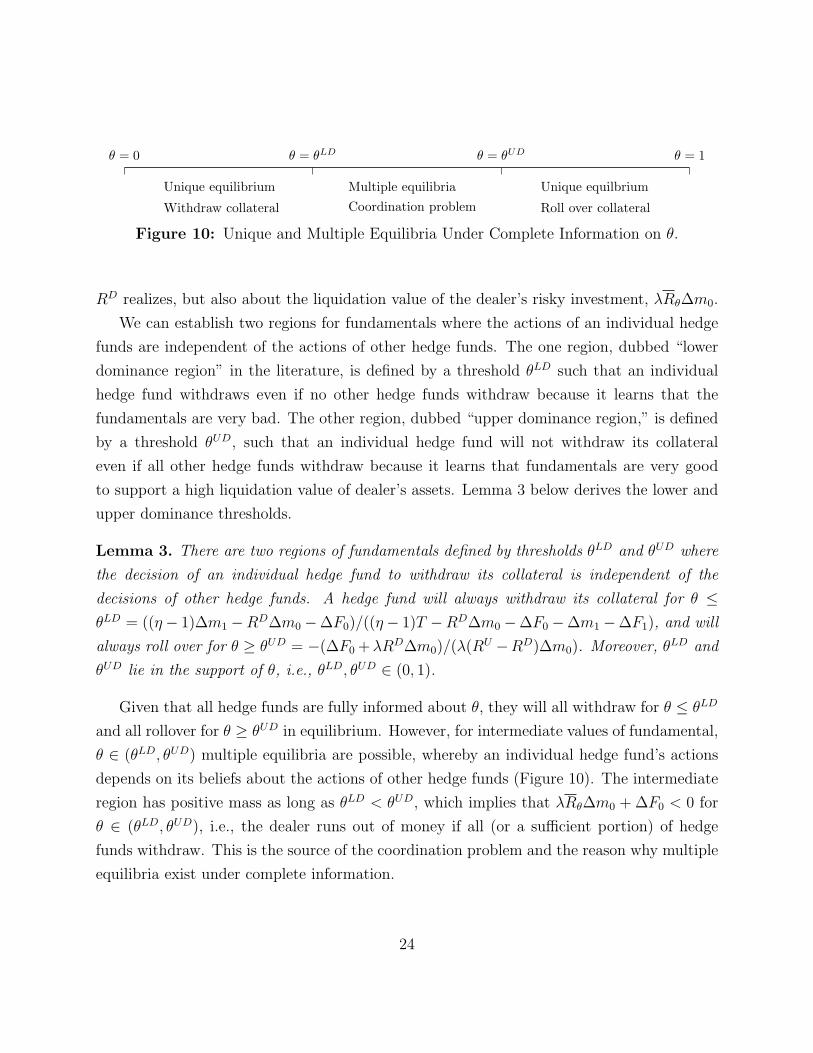
Figure 10: Unique and Multiple Equilibria Under Complete Information on θ.

RD realizes, but also about the liquidation value of the dealer’s risky investment, λRθ∆m0.

We can establish two regions for fundamentals where the actions of an individual hedge

funds are independent of the actions of other hedge funds. The one region, dubbed “lower

dominance region” in the literature, is defined by a threshold θLD such that an individual

hedge fund withdraws even if no other hedge funds withdraw because it learns that the

fundamentals are very bad. The other region, dubbed “upper dominance region,” is defined

by a threshold θUD, such that an individual hedge fund will not withdraw its collateral

even if all other hedge funds withdraw because it learns that fundamentals are very good

to support a high liquidation value of dealer’s assets. Lemma 3 below derives the lower and

upper dominance thresholds.

Lemma 3. There are two regions of fundamentals defined by thresholds θLD and θUD where

the decision of an individual hedge fund to withdraw its collateral is independent of the

decisions of other hedge funds. A hedge fund will always withdraw its collateral for θ ≤

θLD = ((η− 1)∆m1 −RD∆m0 −∆F0)/((η− 1)T −RD∆m0 −∆F0 −∆m1 −∆F1), and will

always roll over for θ ≥ θUD = −(∆F0 +λRD∆m0)/(λ(RU −RD)∆m0). Moreover, θLD and

θUD lie in the support of θ, i.e., θLD, θUD ∈ (0, 1).

Given that all hedge funds are fully informed about θ, they will all withdraw for θ ≤ θLD

and all rollover for θ ≥ θUD in equilibrium. However, for intermediate values of fundamental,

θ ∈ (θLD, θUD) multiple equilibria are possible, whereby an individual hedge fund’s actions

depends on its beliefs about the actions of other hedge funds (Figure 10). The intermediate

region has positive mass as long as θLD < θUD, which implies that λRθ∆m0 +∆F0 < 0 for

θ ∈ (θLD, θUD), i.e., the dealer runs out of money if all (or a sufficient portion) of hedge

funds withdraw. This is the source of the coordination problem and the reason why multiple

equilibria exist under complete information.

24

3.2 Incomplete Information

In order to resolve the coordination problem described in section 3.1, we introduce incomplete

information such that at t = 1, each hedge fund i receives a private noisy signal of the state of

nature xi = θ+ ǫi where the error terms ǫi are independently and uniformly distributed over

[−ǫ, ǫ]. An individual hedge fund’s decision to roll over depends on the signal it receives. The

signal provides information regarding the quality of the risky asset in the dealer’s balance

sheet. In other words it helps inform the probability that the dealer will eventually default

at t = 2 and the hedge fund will forfeit its collateral. The signal also provides information

about other hedge funds’ signals, which allows an inference regarding their actions. An

individual hedge fund may decide to withdraw its collateral not only because it believes that

fundamentals are bad, but also because the conjectured portion of hedge funds withdrawing

is high enough to push the dealer into illiquidity.

We seek a symmetric equilibrium characterized by two thresholds (x∗, θ∗) such that an

individual hedge fund will withdraw its collateral if its private signal realization xi is lower

than a threshold x∗ and the dealer will be fully liquidated at t = 1 if the fundamentals

realization θ is lower than a threshold θ∗.

Under such a threshold strategy, the portion of hedge funds that withdraw their collateral

at a given level of fundamentals θ is

µ(θ, x∗) =

1 if θ < x∗ − ǫ

Prob(xi ≤ x∗|θ) if x∗ − ǫ ≤ θ ≤ x∗ + ǫ

0 if θ > x∗ + ǫ.

(21)

If the fundamental value θ is lower than x∗− ǫ, then all hedge funds receives signals xi < x∗.

Hence, all hedge funds, following a threshold strategy, withdraw and µ(θ, x∗) = 1. The

opposite is true for θ > x∗ + ǫ, whereby all hedge funds roll over and µ(θ, x∗) = 0. Finally, if

fundamentals are not sufficiently higher or lower than x∗, i.e., θ ∈ [x∗− ǫ, x∗+ ǫ], some hedge

funds will receive signals that are lower than x∗ and, thus, will withdraw their collateral.

Given that private noise, ǫi, is independently and identically distributed, from the law of large

numbers the portion of hedge funds withdrawing for a given level of θ in the intermediate

region is µ(θ, x∗) = Prob(xi ≤ x∗|θ) = (x∗ − θ + ǫ)/2ǫ.

The signal and fundamentals thresholds are derived in two steps as follows. First, given

25

the threshold strategy x∗, we can derive the threshold for fundamentals, θ∗, which determines

whether the dealer is fully liquidated at t = 1 or survives to t = 2. Because the portion of

hedge funds withdrawing is decreasing in θ from (21), the dealer is fully liquidated only if

θ < θ∗ where θ∗ is the unique solution to f(µ(θ∗, x∗), θ∗) = 1 given by equation (4):

θ∗ = x∗ − ǫ∆m1 + 2∆F0 + 2λRθ∗∆m0

∆m1

. (22)

In other words, for threshold strategy x∗, if θ is lower than θ∗, then the portion of hedge

funds withdrawing is higher than what the dealer can serve by liquidating her assets and

f(µ(θ, x∗), θ) < 1. On the contrary, if θ is higher than θ∗, fewer hedge funds withdraw,

allowing the dealer to decrease asset liquidations and survive to t = 2.14

Second, given the fundamentals threshold θ∗, an individual hedge fund can compute the

signal threshold x∗, below which it is optimal to withdraw conditional on its expectation

over the portion of hedge funds withdrawing and the private signal it receives. This signal

threshold depends on the utility differential between rolling over and withdrawing for a

given level of θ and µ. The difference in expected payoff is given by UH(µ, θ; a = 1)-

UH(µ, θ; a = 0) derived from (12)-(17). Given that in equilibrium FMt = T and mM

t = 0,

the utility differential ν(µ, θ) is given by the following piecewise function:

ν(µ, θ) =

θ [(η − 1)T −∆F1] + (1− θ)GDS (µ, θ)− η∆m1 µ ∈ [0, µS)

θ [(η − 1)T −∆F1] + (1− θ)GDI (µ, θ)− η∆m1 µ ∈ [µS, µI)

θGUI (µ, θ) + (1− θ)GD

I (µ, θ)− η∆m1 µ ∈ [µI , µR)

−η λRθ∆m0+∆F0+∆m1

µµ ∈ [µR, 1]

(23)

whereGDS (µ, θ) =

(RD∆m0 +∆F0 + (1− µ)∆m1

)/ (1− µ), GD

I (µ, θ) = (RD∆m0+RD/λRθ·

(∆F0 + (1− µ)∆m1))/(1− µ), and θGUI (µ, θ) + (1− θ)GD

I (µ, θ) = (Rθ∆m0 + 1/λ · (∆F0 +

(1− µ)∆m1))/(1− µ) from (6), (9) and (10).

We plot the utility differential ν(µ, θ) for a certain level of θ in Figure 11. Looking at the

two first legs, the payment in the bad state for a hedge fund that rolled over is decreasing in

14The fraction of assets distributed is strictly decreasing in µ, i.e., ∂f(µ, θ)/∂µ = (λRθ∆m0 + ∆F0 +∆m1)/(µ

2∆F0) < 0 given condition in equation (1).

26

µ and limµ→µS− GD

S (µ, θ) = limµ→µS+ GD

I (µ, θ).15 The third leg is also decreasing in µ for

λRθ∆m0 +∆F0 < 0, i.e., for θ < θUD. The utility differential is discontinuous at µI because

the hedge fund fails to receive the non-pecuniary benefit η if the dealer defaults. However,

limµ→µI− ν(µ, θ)− limµ→µI

+ ν(µ, θ) = θ(η − 1)T > 0, and, thus, ν(µ, θ) is strictly decreasing

in µ ∈ [0, µR) for θ < θUD which is the relevant region where a coordination problem may

occur. The final leg in (23) is increasing in µ given that λRθ∆m0+∆F0+∆m1 > 0 from the

condition in equation (1). Thus, the model features one-sided, rather than global, strategic

complementarities as in Goldstein and Pauzner (2005). Once the dealer is fully liquidated, a

hedge fund has fewer incentives to withdraw as withdrawals increase. Note that ν “crosses”

zero as µ increases from above. That is, depending on the contract terms, this can happen

within any of the first two legs or at the jump, but not within the third and fourth legs

where ν(µ, θ) always takes negative values.16

Consider an individual hedge fund that receives signal xi. The hedge fund will use the

signal to update its beliefs about the realization of θ. Given that both θ and ǫi are uniformly

distributed, the posterior distribution of θ given xi is θ|xi ∼ U [xi−ǫ, xi+ǫ]. This implies that

the utility differential between rolling over and withdrawing for a hedge fund that receives

signal xi as a function of the cutoff value is

∆(xi, x∗) =

1

2ǫ

∫ xi+ǫ

xi−ǫ

ν(µ(θ, x∗), θ)dθ. (24)

In a threshold equilibrium, a hedge fund prefers to withdraw, i.e., ∆(xi, x∗) < 0, for all

xi < x∗, and prefers to roll over, i.e., ∆(xi, x∗) > 0, for all xi > x∗. ∆(xi, x

∗) is continuous

in xi because a change in the signal only changes the limits of integration [xi − ǫ, xi + ǫ] and

the integrand is bounded. Hence, a hedge fund that receives signal xi = x∗ is indifferent

between rolling over and withdrawing, i.e.,

∆(x∗, x∗) =1

2ǫ

∫ x∗+ǫ

x∗−ǫ

ν(µ(θ, x∗), θ)dθ = 0. (25)

15∂GDS (µ, θ)/∂µ = (RD∆m0 +∆F0)/(1− µ)2 < 0, because RD < 1 and ∆m0 +∆F0 < 0 from Lemma 2,

while ∂GDI (µ, θ)/∂µ = RD/(λRθ(λRθ∆m0 +∆F0)/(1− µ)2 < 0 for θ < θUD.

16ν(µ, θ) < 0 for µ ∈ [µI , µR) —third leg— requires µ > 1+(λRθ∆m0+∆F0)/∆m1 > µI , which is alwaystrue.

27

µS µI

0

µRµ

ν

Figure 11: Indifference Function ν(µ, θ) as a Function of µ for Arbitrary θ ∈ (θLD, θUD)and Arbitrary Contract Terms.

Equations (22) and (25) jointly determine the threshold for fundamentals θ∗ and the

threshold strategy x∗. Proposition 1 establishes the existence and uniqueness of a threshold

equilibrium.17

Proposition 1. Given contract terms satisfying θLD < θUD in Lemma 3, there exist a

threshold, x∗, such that a hedge fund rolls over if xi > x∗ and withdraws if xi < x∗, and a

threshold θ∗, such that the dealer does not experience any withdraws if θ ≥ θ∗ and is fully

liquidated if θ < θ∗. Moreover, the thresholds are unique if noise is not too large.

Hereafter, we focus on the case that the noise goes arbitrarily close to zero. Taking

the limit ǫ → 0 implies that x∗ → θ∗ from (22). A hedge fund that receives signal x∗,

the posterior distribution of θ is uniform over the interval [x∗ − ǫ, x∗ + ǫ]. Thus, that hedge

17As already mentioned, the model features one-sided strategic complementarities. Hence, we follow thesteps in Goldstein-Pauzner and make the same assumptions, most importantly that noise is uniformly dis-tributed, to show the uniqueness of a threshold equilibrium. However, our framework features two additionalcomplications. First, due to limited liability, the dealer’s default threshold is endogenous. Second, the liqui-dation value matters for the payoff in a run and, thus, state monotonicity of ν(µ, θ) is not straightforward.We explicitly address these complications in the proof of Proposition 1. But to simplify the analysis werestrict attention to a uniformly distributed probability of a good realization, while Goldstein-Pauzner allowfor more general distributions of the probability of a good realization, p(θ), where θ is uniformly distributedand p′(θ) > 0. In our case, p(θ) = θ and p′(θ) = 1.

28

fund’s belief of the portion of hedge funds withdrawing as a function of θ, µ(θ, x∗), is uniform

over [0, 1].18 In other words, as θ decreases from x∗ + ǫ to x∗ − ǫ, µ increases from 0 to 1.

Changing variables in ∆(x∗, x∗) = 0 provides the indifference condition that determines the

unique value θ∗:

V (θ∗) =

∫ 1

0

ν(µ, θ∗)dµ = 0. (26)

The detailed expression for V (θ∗), with its derivatives with respect to θ∗ and the contract

terms, are shown in equation (B.28) in Appendix B. Moreover, (26) implies that ν(0, θ∗) > 0

given that ν is decreasing in µ when positive, which can be used to establish the following

Corollary.

Corollary 1. The period 1 participation constraint (19) is always slack for all θ ≥ θ∗.

Contrary to the complete information case, the introduction of noisy private signals

eliminates the possibility of multiple equilibria in the intermediate region of fundamentals,

i.e., θ ∈ (θLD, θUD). The dealer is fully liquidated for θ < θ∗. Figure 12 shows the regions

where full liquidation (a “run”) occurs. The region of θ below the threshold θLD corresponds

to a fundamental run similar to the complete information case. The region between θLD and

θ∗ corresponds to a panic-based run due to dealer illiquidity. The overall run probability is

equal to Prob(θ < θ∗), and can be split between a fundamental run probability, Prob(θ <

θLD), and a panic-based run probability, Prob(θLD ≤ θ < θ∗).

θ = 0

Fundamental run

θ = θLD

Panic-based run

θ = θ∗

No run

θ = θUD

No run

θ = 1

Figure 12: Unique equilibrium under Incomplete Information on θ.

4 Threshold Equilibrium

Having characterized hedge funds’ threshold strategy under incomplete information, we turn

to see the effective take-it-or-leave-it contracting terms the dealer chooses, anticipating hedge

18This is true because limx∗→θ∗ Prob(µ(θ, x∗) ≤ N) = Prob(µ(θ, θ∗) ≤ N) = 1−Prob(θ ≤ θ∗+ǫ−2ǫN) =1− (θ∗ + ǫ− 2ǫN − θ∗ + ǫ)/(2ǫ) = N . Hence, µ(θ, θ∗) ∼ U [0, 1].

29

funds’ optimal strategy. Because a hedge fund’s problem is scalable, we normalize T = 1

for simplicity. This implies that feasible contract terms should satisfy ∆mt ∈ [0, 1] and

∆Ft ∈ [−1, 0].

Given threshold for fundamentals θ∗ defined in (26), all hedge funds withdraw their

collateral for θ < θ∗, inducing the dealer to default and receive zero profits. Conversely, if

the realization of θ is above θ∗ all hedge funds roll over their repos to period t = 2 and the

dealer is exposed to the risky asset’s payoff. With probability θ, the good state realizes and

the dealer enjoys positive profits. Otherwise, the bad state realized and the dealer defaults

receiving nothing. Her expected utility is, then, given by:

UD =

∫ θ∗

0

θu(0)dθ +

∫ 1

θ∗

[θu(RU∆m0 +∆m1 +∆F0 +∆F1) + (1− θ)u(0)

]dθ

=(1− θ∗2)

2u(RU∆m0 +∆m0 +∆F0 +∆F1), (27)

where u(·) is a concave utility function–not excluding linear utility–with u(0) = 0.19.

The dealer will internalize that changing the contracting terms directly affects hedge

funds’ threshold strategy θ∗ through the “global game” condition (26), and, thus, the prob-

ability of a collateral run. In many global games applications, the run threshold can derived

in closed-form using a condition similar to (26). Given the complexity herein, we are not able

to solve for the threshold in closed-form to substitute it in the dealer’s problem.20 Instead,

we will explicitly impose (26) as a constraint that the dealer faces and have her optimize

also over θ∗ respecting its relationship with the other contract terms.

Hence, the dealer chooses ∆m0,∆m1,∆F0,∆F1, θ∗ to maximize (27) subject to the

period-0 hedge funds participation constraint (18), the global game constraint (26), the

19It is important to note that a coordination problem can exist only if ∆m0 > 0. If hedge funds donot have an unsecured claim on the dealer, i.e., ∆m0 = 0, there cannot be an advantage to withdrawearly. This situation can be appreciated graphically through Figure 8 and 9: if there is nothing hedgefunds’ can claim, beyond their collateral, there is no reason to withdraw. In this case the dealer would notinvest in the risky asset, and the only feasible contracting terms that give dealer non-negative profits are∆m0 = ∆m1 = ∆F0 = ∆F1 = 0, i.e., u(0) = 0. This implies that the dealer is better off setting contractingterms that expose her to a run as long as the profits in the good state are positive and θ∗ < 1

20A closed-form solution is attainable in Goldstein and Pauzner (2005) because the liquidation value doesnot depend on fundamentals. In Rochet and Vives (2004), the liquidation value depends on fundamentals,but the payoff structure does not, allowing for a closed-form solution.

30

positive liquidity injection constraint (1), and the bad-state default constraint (7).21 We

have imposed the last constraint in the dealer’s problem to guarantee the existence of a

lower dominance region, which is essential for the existence of a threshold equilibrium in

the incomplete information game. Note that the coordination failure examined in this paper

would be present even without the lower dominance region. Instead of imposing default in

the bad-state, one could consider equilibrium refinements that give rise to the same threshold

strategy. We will elaborate further on the presence of these four constraints below, after we

have established the existence of contract terms that give rise to a coordination problem

and, hence, the possibility of collateral runs.22

Proposition 2. For λRU > 2, RD < ηRU/(η + RU), and dealer’s risk-aversion not suffi-

ciently low, there exist optimal contracting terms ∆mt(θ∗) and ∆Ft(θ

∗) under which hedge

funds adopt a threshold strategy θ∗.

Note that the existence result in Proposition 2 requires a high degree of dealer risk

aversion so that that the marginal utility of the dealer is low enough to push θ∗ to its upper

bound θUD. In other words, conditional on survival at θUD the dealer would prefer a lower

run probability over higher profits in the good state. As we will see in the following corollary,

this can be true when the dealer is risk-neutral, but under stricter parameter conditions.

The optimal contracting terms of Proposition 2 are only a function of the threshold θ∗

and given by ∆m0(θ∗) = −θ∗(η− 1)µI/f(θ

∗), ∆m1(θ∗) = g(θ∗)∆m0(θ

∗), ∆F0(θ∗) = −g(θ∗),

∆m0(θ∗), and ∆F1(θ

∗) = −RD∆m0(θ∗), where g(θ∗) and f(θ∗) are given by (20) and (A.25),

respectively. Finally, the run threshold is the solution to the following optimization condition:

1

2(1− θ∗2)u′((RU −RD)∆m0(θ

∗))(RU −RD) +θ∗u

((RU −RD)∆m0(θ

∗))f(θ∗)

∂V∂θ∗

−∆m0(θ∗)g′(θ∗)(

∂V∂∆F0

− ∂V∂∆m1

) = 0,

(28)

which can be easily interpreted. The first term captures the incremental utility to the dealer

21Alternatively, the problem can be stated with θ∗ determined implicitly, and the dealer internalizing howcontracting terms change the threshold. These approaches are mathematically equivalent.

22The participation constraint in period one is always slack from Corollary 1, and the contract terms willbe interior. Thus, for the sake of conciseness, we do not include (19), 0 ≤ ∆mt ≤ 1 and −1 ≤ ∆Ft ≤ 0 inthe dealer’s optimization problem. The Lagrangian and the first-order optimization conditions are reportedin (A.18)-(A.23) in Appendix A.

31

from an increase in the initial risky investment while keeping the run probability unchanged.

The second term captures the effect on the probability that the dealer suffers a run, and,

hence, forfeits any profits in the final period (note that the term is negative). So, the dealer

balances the higher profits conditional on a run not occurring, with the associated increase

in the probability of a run.

The optimal contracting terms of Proposition 2 are characterized by four binding con-

straints: the global game constraint, the initial participation constraint, the positive liquidity

injection constraint, and the dealer default constraint. The last three constraints allow us to

write the contract terms ∆F0, ∆m1, and ∆F1 as function of ∆m0 and θ∗. The first one gives

∆m0 as a function of θ∗. As already mentioned, the global game and initial participation

constraints will always be binding. We, now, discuss in more detail the intuition behind the

other two binding constraints.

The binding liquidity injection constraint implies that the dealer does not collect any net

funds in t = 1. The intuition behind the tightness of this restriction stems from inspecting

θ∗’s sensitivity to both ∆m1 and ∆F0. To see this, consider contracting terms which do not

have a binding PC0 constraint. In that case, the only difference between ∆m1 and ∆F0 is how

those variables affect θ∗. In the proposed equilibrium we have, ∂θ∗/∂∆m1−∂θ∗/∂∆F0 > 0.23

Intuitively this is because a hedge fund loss due to an increase in ∆m1 only affects hedge

funds that roll over. A hedge fund loss due to an increase in ∆F0 is mutualized between

those that roll over and those that do not. That is, the dealer gets more “bang for her buck”

by altering the roll over haircut. Thus, to increase the possibility for hedge funds to rollover

(i.e., lower θ∗), it is optimal to reduce hedge funds’ loss via a reduction in ∆m1 rather than

∆F0, which is pinned down by the initial participation constraint.

Interestingly, the choice of ∆m1 versus ∆F0 highlights a tradeoff which can be lost without

considering hedge fund’s rollover decision. Given that the sum of these two contracting terms

results in the effective net payment from hedge funds that roll over, their direct marginal

impact on the dealer’s utility is identical. The difference stems from considering how these

contracting terms affect the marginal hedge fund’s decision to roll over or not. In this regard,

the contracting terms are very different, because ∆F0 is paid by all whereas ∆m1 is only

23From the implicit function theorem ∂θ∗/∂∆m1 − ∂θ∗/∂∆F0 = (∂V/∂∆F0 − ∂V/∂∆m1)(∂V/∂θ∗)−1.

∂V/∂∆F0 − ∂V/∂∆m1 pins down the value of the multiplier on the participation constraint (see (A.26)),and thus is positive. Given that ∂V/∂θ∗ > 0 from the proof of Proposition 1, ∂θ∗/∂∆m1 − ∂θ∗/∂∆F0 ispositive as well.

32

paid by those who continue.

The final active constraint is the dealer’s default condition. The intuition behind this

active constraint is that an increase in ∆F1 affects the dealer’s payoff directly with a minimal

impact on the sensitivity of θ∗: It has a small impact on µI , and only affects the final

repayment of hedge funds’ that roll over directly, with no effect on the incentives between

rolling over and withdrawing. This is why in equilibrium the dealer decides to set contracting

terms in which she is on the verge of defaulting in the bad state.

Having a general characterization of the equilibrium in Proposition 2 we focus on a

specific case that gives a more precise characterization of the equilibrium outcome, and also

allows us to do comparative statics. Specifically, we shall assume that the risky asset payoff

is zero in the down state RD = 0 and the dealer is risk neutral. In this case, we have the

following result,

Corollary 2. For RD = 0, λRU ∈(

2, 4+8√2

7

)

, and risk neutral dealer, there exist optimal

contracting terms

∆m0(θ∗) = θ∗(η−1)

ηg(θ∗)

(

1−ln

(

λRθg(θ)

)) , ∆m1(θ∗) = g(θ∗)∆m0(θ

∗)

∆F0(θ∗) = −g(θ∗)∆m0(θ

∗), ∆F1(θ∗) = 0

under which hedge funds adopt a threshold strategy θ∗ that solves,

2

(

1− θ∗ − 3θ∗2 + θ∗(1 + θ∗)λRθ∗

g(θ∗)

)

= ln

(λRθ∗

g(θ∗)

)(

1− θ∗ − 4θ∗2 + θ∗(1 + θ∗)λRθ∗

g(θ∗)

)

with ∂θ∗

∂RU < 0.

The optimal contracting terms have the same functional form as in Proposition 2 with

many of the expressions simplified, because in this case µI = µR. Since RD = 0, the no

default condition can be replaced by the reasonable restriction of having the ∆F1 ≤ 0. If

this were not the case, the dealer would never default.

Note that we present the comparative statics with respect to RU , but these are identical

to the ones with respect to λ.24 As the asset becomes more valuable at liquidation, either

24With dealer risk aversion this would not be the case, because the dealer’s marginal utility is affected bythe final payoff (see equation (28)).

33

due to a higher payment on the good state or a lower liquidity discount, the possibility of a

run becomes smaller. That is, the dealer would have more funds to compensate hedge funds

in case they were to withdraw, reducing their incentives to do so.

Changes in η do not affect the equilibrium threshold, again because of the dealer’s risk

neutrality. But changes in η do materially change the optimal contrasting terms. As hedge

funds have higher profits through their preference for holding safe assets, the initial repo

margin ∆m0 can be higher.

The following subsection presents a numerical example of the model’s comparative statics

whenever the dealer is risk averse and the asset value is positive in the down state.

4.1 Numerical Example

Proposition 2 characterizes equilibria which we can calculate numerically. Figure 13 shows

the hedge fund’s utility differential under the optimal strategies for one particular set of

parameters. As stated in the equilibrium of Proposition 2, it’s optimal for the dealer not to

collect any additional payments in the interim period ∆m0 +∆F1 = 0 =⇒ µS = 0. As with

all threshold equilibria, we have that µI < µR < 1.

Figure 14 shows how the equilibrium threshold θ∗, and its associated upper and lower

dominance, change with model parameters. The interpretation of the top two and bottom

right panels shows that as the assets unconditional liquidation value increases, the possibility

of a threshold strategy is smaller. In particular, the interval with panic-based runs (i.e.,

(θLD, θ∗) shrinks. This might seem like a beneficial outcome: it is less likely to have a panic

based equilibrium. In addition, the range where both panic-based and fundamental runs is

also smaller (i.e., (0, θ∗)).

But changes in η shows that there are cases where the panic-based equilibrium interval

is larger, while both panic-based and fundamental runs are overall smaller. That is, in these

cases, the larger coordination problem in fact decreases the probability of a run, highlighting

the case where coordination can be helpful.

34

µI µRµ

ν

0

Figure 13: Marginal Hedge Funds Indifference Function νFigure shows the indifference function ν of the optimal contract for a marginal HedgeFund with a safe asset valuation of η = 5, asset parameters RU = 2, RD = 0.5, λ = 0.8,and the Dealer with with CARA utility, risk aversion γ = 5. Dashed red line highlightswhere ν crosses zero.

The numerical exercise also highlights how contracting terms change as the equilibrium

changes with underlying parameters. For illustration purposes, Figure 15 shows the equilib-

rium haircuts (top panel) and equilibrium interest rates (bottom panel) in t=0 and t=1 as

a function of the equilibrium θ∗ for different values of RD. The top panel shows that the

haircut in t = 0 is lower than the haircut in t = 1. This is merely a graphical representation

of Lemma 2 and stems from the fact that −∆F0 > ∆m0, so as to compensate hedge funds to

participate initially, and in equilibrium there is no liquidity injection ∆m1 = −∆F0. That

is, even though there is no transfer of payments in t = 1, observing haircuts in isolation gives

an increase in haircuts from the initial to rollover period. This can change the interpretation

of an increase in haircuts: dealers may not be putting more onerous contracting terms to

their counterparties, but rather they just reviving enough funds to pay off existing contracts.

The bottom panel shows that the interest rate in t = 0 is lower that the interest rate

in t = 1. Moreover, the interest rate in t = 0 is negative, indicating dealers are willing to

get a negative return when contracting with hedge funds to incentivize them to participate.

This is somewhat similar to a well-known market outcome when there is high demand for

35

0.1 0.15 0.2 0.25 0.3 0.35 0.4 0.45 0.5 0.55 0.60.25

0.3

0.35

0.4

0.45

0.5

0.55

0.6

0.65

0.7

2 2.2 2.4 2.6 2.8 3 3.20.3

0.35

0.4

0.45

0.5

0.55

0.6

0.65

0.7

0.75

2 2.5 3 3.5 4 4.5 50.32

0.34

0.36

0.38

0.4

0.42

0.44

0.46

0.48

0.5

0.68 0.7 0.72 0.74 0.76 0.78 0.8 0.82 0.84 0.86 0.880.25

0.3

0.35

0.4

0.45

0.5

0.55

0.6

0.65

0.7

θθ

θθ

θ∗θ∗

θ∗θ∗

θUDθUD

θUDθUD

θLDθLD

θLDθLD

η λ

RD RU

Figure 14: Changes in θ∗ for Different Model ParametersFigure shows how the threshold strategy changes with different underlying parameters(solid blue line). The figure also shows how the upper dominance (dashed red line) andlower dominance (dotted green line) thresholds change. Equilibria are around the initialparameter valuations of η = 5, RU = 2.5, RD = 0.5, λ = 0.8, and the dealer with CARAutility, risk aversion γ = 5.

36

0.385 0.39 0.395 0.4 0.4050.16

0.18

0.2

0.22

0.24

0.26

0.28

0.3

0.32

0.34

0.385 0.39 0.395 0.4 0.405-0.1

-0.05

0

0.05

0.1

0.15

0.2

0.25

0.3

mH

r

θ∗

θ∗

r0r1

m0

m1

Net Interest Rates in t = 0 and t = 1

Haircuts in t = 0 and t = 1

Figure 15: Changes in Contracting Terms as Equilibrium Changes with RD

Figure shows how contracting terms change as the equilibrium changes for different valuesof RD. Equilibria are with a safe asset valuation of η = 5, asset parameters RU = 2.5,RD ∈ [0.1, 0.64], λ = 0.8, and the Dealer with CARA utility, risk aversion γ = 5.

a particular asset, known as repo specialness. In this context, the safe asset is not trading

special because counterparties need to source collateral for short positions, but rather because

the dealer can make a profit by purchasing a risky asset position with liquidity stemming

from rehypothecation.

5 Conclusion

This paper presents a model which highlights fragility that can arise from the re-use of

collateral in a short-term collateralized lending context. Specifically, the paper characterizes

a coordination failure that can arise amongst cash borrowers, inducing a panic-based default

on an intermediary. In contrast to traditional wholesale funding runs, the model shows

that when intermediating secured financing fragility can materialize on the asset side of an

37

intermediary’s balance sheet. The model delivers a unique threshold equilibria in which

panic-based runs can ensue. In addition, the paper shows how different repo contracting

terms, specifically the haircut and repurchase price, can have a differential effects on collateral

providers’ incentives to run. This provides another mechanism in which to disentangle

different repo contracting terms.

The results in this paper also pose a challenge for regulators concerned with the fragility

of large broker dealers. Much of the regulation introduced since the 2007–09 is designed to

monitor and restrict the composition of banks liabilities. This paper cautions that this focus

is too narrow. Given that the total amount of collateral received is an important source of

liquidity, fragility can present itself on the asset side of bank’s balance sheet, as well.

References

Acharya, V. V., Gale, D. and Yorulmazer, T. (2011), ‘Rolloever risk and market freezes’,

Journal of Finance 66(4), 1177–1209.

Ahnert, T. (2016), ‘Rollover risk, liquidity and macroprudential regulation’, Journal of

Money, Credit and Banking 48(8), 1753–1785.

Bebchuk, L. A. and Goldstein, I. (2011), ‘Self-fulfilling credit market freezes’, Review of

Financial Studies 24(11), 3519–3555.

Bond, P. and Rai, A. S. (2009), ‘Borrower runs’, Journal of Development Economics

88(2), 185 – 191.

URL: http://www.sciencedirect.com/science/article/pii/S0304387808000667

Brunnermeier, M. K. and Pedersen, L. H. (2009), ‘Market liquidity and funding liquidity’,

Review of Financial Studies 22(6), 2201–2238.

Carlsson, H. and van Damme, E. (1993), ‘Global games and equilibrium selection’, Econo-

metrica 61(5), 989–1018.

Chen, Q., Goldstein, I. and Jiang, W. (2010), ‘Payoff complementarities and financial

fragility: Evidence from mutual fund outflows’, Journal of Financial Economics 97(2), 239

– 262.

38

Copeland, A., Martin, A. and Walker, M. (2014), ‘Repo runs: evidence from the tri-party

repo market’, The Journal of Finance 69(6), 2343–2380.

Diamond, D. W. and Dybvig, P. H. (1983), ‘Bank runs, deposit insurance, and liquidity’,

Journal of Political Economy 91(3), 401–419.

Diamond, D. W. and Rajan, R. G. (2011), ‘Fear of fire sales, illiquidity seeking, and credit

freezes’, Quarterly Journal of Economics 127(2), 557–591.

Duffie, D. (2013), ‘Replumbing our financial system: Uneven progress’, International Journal

of Central Banking 9(1), 251–279.

Fostel, A. and Geanakoplos, J. (2008), ‘Leverage cycles and the anxious economy’, American

Economic Review 98(4), 1211–1244.

Fostel, A. and Geanakoplos, J. (2015), ‘Leverage and default in binomial economies: A

complete characterization’, Econometrica 83(6), 2191–2229.

Geanakoplos, J. (2003), ‘Liquidity, default, and crashes: Endogenous contracts in general

equilibrium’, Advances in Economics and Econometrics: Theory and Applications, Eighth

World Conference, Volume II, Econometric Society Monographs pp. 170–205.

Goldstein, I. and Pauzner, A. (2005), ‘Demand-deposit contracts and the probability of bank

runs’, Journal of Finance 60(3), 1293–1327.

Gorton, G. B. and Metrick, A. (2012), ‘Securitized banking and the run on repo’, Journal

of Financial Economics 104(3), 425–451.

He, Z. and Xiong, W. (2012), ‘Dynamic debt runs’, Review of Financial Studies 25(6), 1799–

1843.

Huh, Y. and Infante, S. (2017), ‘Bond market liquidity and the role of repo’.

Infante, S. (2017), ‘Liquidity windfalls: The consequences of repo rehypothecation’.

Kashyap, A. K., Tsomocos, D. P. and Vardoulakis, A. P. (2017), ‘Optimal bank regulation

in the presence of credit and run risk’, Working Paper .

39

Krishnamurthy, A., Nagel, S. and Orlov, D. (2014), ‘Sizing up repo’, The Journal of Finance

69(6), 2381–2417.

Liu, X. and Mello, A. S. (2011), ‘The fragile capital structure of hedge funds and the limits

to arbitrage’, Journal of Financial Economics 102(3), 491 – 506.

Martin, A., Skeie, D. and Von Thadden, E.-L. (2014), ‘Repo runs’, Review of Financial

Studies 27(4), 957–989.

Morris, S. and Shin, H. (1998), ‘Unique equilibrium in a model of self-fulfilling currency

attacks’, American Economic Review 88(3), 587–597.

Morris, S. and Shin, H. S. (2004), ‘Coordination risk and the price of debt’, European Eco-

nomic Review 48(1), 133–153.

Rochet, J.-C. and Vives, X. (2004), ‘Coordination failures and the lender of last resort: Was

bagehot right after all?’, Journal of the European Economic Association 2(6), 1116–1147.

Simsek, A. (2013), ‘Belief disagreements and collateral constraints’, Econometrica 81(1), 1–

53.

Vives, X. (2014), ‘Strategic complementarity, fragility and regulation’, Review of Financial

Studies 27(12), 3547–3592.

40

Appendices

A Proofs

Proof of Lemma 1

For values of θ such that a run of the dealer is possible, i.e., µR < 1, or equivalently ∆F0+λRθ∆m0 < 0,

the default threshold, µI , is always lower than the run threshold, µR, if λRθ∆F1 + RU∆m1 > 0. The

latter expression can be written as λRθ∆F1 + RU∆m1 > (RU∆m0∆m1 − ∆F0∆F1)/∆m0 using the fact

that ∆F0 + λRθ∆m0 < 0 and ∆F0,∆F1 < 0. Given that ∆m1 ≥ −∆F0 from condition C0 in (1),

RU∆m0∆m1 −∆F0∆F1 > −∆F0(RU∆m0 +∆F1) > 0, using condition C2 in (8).

Finally, to ensure that the dealer will begin to sell before it comes insolvent, i.e., µS < µI , we also need

RU∆m1∆m0 −∆F1∆F0 > 0, which we proved above.

Proof of Lemma 2

From (18) we get that:

−∆F0

[∫ 1

θ∗

dθ +

∫ θ∗

0

f(1, θ)dθ

]

≥ ∆m0 ⇒ −∆F0 > ∆m0, (A.1)

because∫ 1

θ∗dθ +

∫ θ∗

0f(1, θ)dθ < 1. This proves claim 1.

Combining (A.1) and (1), we get that ∆m1 > ∆m0. This proves claim 2.

Proof of Lemma 3

The lower dominance region is defined by the values of θ for which an individual hedge fund chooses to

withdraw even if other hedge funds do not. The utility differential between rolling over and withdrawing

when µ = 0 from (12) and (16) is UH(0, θ; 1)− UH(0, θ; 0) = θ[(η − 1)T −∆F1] + (1− θ)[RD∆m0 +∆F0 +

∆m1] − η∆m1, where we have substituted the equilibrium conditions FMt = T and mM

t = 0 derived in

section 2.3. Given that the differential is increasing in θ the lower dominance region comprises of values for

θ ≤ θLD, where θLD is the solution to UH(0, θLD; 1)− UH(0, θLD; 0) = 0, i.e.,

θLD =(η − 1)∆m1 −RD∆m0 −∆F0

(η − 1)T −RD∆m0 −∆F0 −∆m1 −∆F1.

The lower dominance threshold θLD is greater than zero because, from Lemma 2 and RD < 1, RD∆m0 +

∆F0 < (RD − 1)∆m0 < 0, and from condition (7) RD∆m0 +∆F0 +∆m1 +∆F1 < 0. It is also lower than

one because (η − 1)T −∆F1 > η∆m1 from the period 1 participation constraint (19).

The upper dominance region is defined by the values of θ for which an individual hedge fund rolls over

even if all other hedge funds withdraw. First, we need to guarantee that for θ ≥ θUD, the dealer has enough

liquidity to serve all early withdraws, i.e., λRθ∆m0 +∆F0 ≥ 0. Given that the last expression is increasing

41

in θ, the upper dominance threshold is the root, i.e.,

θUD = −∆F0 + λRD∆m0

λ(RU −RD)∆m0.

The upper dominance threshold θUD is greater than zero because, from Lemma 2 and λRD < 1, ∆F0 +

λRD∆m0 < (λRD − 1)∆m0 < 0. To show that θUD is lower than one, we impose a binding partic-

ipation constraint (18), which is always the case under the equilibrium contract terms. Then, θUD =

(g(θ∗) − λRD)/(λRU − λRD), where g(θ∗) is given by (20), and is smaller than one if g(θ∗) < λRU .

Substituting the expression for g(θ∗), the latter condition can be written as X (θ∗) ≡ λ(RU − RD)θ∗2 −

2λ(RU − RD)θ∗ + 2(λRU − 1) > 0. X does not have real roots because the discriminant 4λ(RU −

RD)[λ(RU −RD)− 2(λRU − 1)

]< 0 given the restriction λ(RU +RD)/2 > 1.

We have shown that for θ ≥ θUD, the hedge fund believes the liquidation price is high enough to avoid a

liquidity default. Now we must ensure that the hedge fund in fact wants to roll over. To conclude the proof,

we need to show that for θ ≥ θUD and µ → 1, the utility differential between rolling and withdrawing for

an individual hedge fund is positive. Technically, we need to check whether an infinitesimal hedge fund with

mass ε that deviates from the strategy of other fund that withdraw can repurchase its collateral at t = 2. In

other words, we need to check whether the dealer default on the remaining −ε∆F1 obligations when ε → 0.

The dealer will not default if the value of her remaining asset is higher that her remaining obligations, i.e.,

limµ→1 GUI (µ, θ)/(−∆F1) > 1 with GU

I (µ, θ) given by (10). Changing variables such that µ = 1 − ε and

substituting λRθ∆m0 = λRθUD∆m0 +Ω(θ)∆m0, where Ω(θ) ≥ 0 because θ ≥ θUD, we get that:

limε→0

GUI (1− ε, θ)

−∆F1=−

RU

λRθ

limε→0

λRθUD∆m0 +Ω(θ)∆m0 +∆F0 + ε∆m1

ε∆F1

= −RU

λRθ

∆m1

∆F1+

Ω(θ)∆m0

∆F1limε→0

1

ε,

where we used the fact that λRθUD∆m0+∆F0 = 0 from the definition of θUD. Given that limε→0Ω(θ)∆m0

ε∆F1

→

∞ for θ > θUD, it suffices to show that for θ = θUD, i.e., Ω(θ) = 0 irrespective of the value of ε, the limit

converges to a value higher than 1. Using λRθUD∆m0 + ∆F0 = 0, we get that the limit converges to

−(RU∆m1/(λRθUD∆F1) = RU∆m0∆m1/(∆F0∆F1), which is greater than 1 because, as proved in Lemma

1, RU∆m0∆m1 − ∆F0∆F1 > 0. Hence, the dealer will not default at t = 2 if RU realizes and the hedge

fund will be able to repurchase its collateral.

If, instead RD realizes at t = 2, the limit is

limε→0

GUI (1− ε, θ)

−∆F1= −

RD

λRθ

∆m1

∆F1+

Ω(θ)∆m0

∆F1limε→0

1

ε.

Again, for the θ > θUD, the second term goes to infinity and the dealer does not default. But, for θ = θUD,

the limit goes to −(RD∆m1/(λRθUD∆F1) = RD∆m0∆m1/(∆F0∆F1). Using conditions (1) and (7) we get

that RD∆m0 + ∆F1 < 0 and, hence, the limit is higher than 1 for ∆m1 > ∆F0∆F1/(RD∆m0) > −∆F0

42

and less than one otherwise. If the former case, the dealer does not default and the hedge fund is able to

repurchase its collateral. In the latter case, the dealer defaults and the hedge fund gets −RD∆m1∆m0/∆F0.

In most cases described above the dealer does not default either in the good or in the bad state and it is

straightforward that the hedge fund’s period 1 participation constraint (19) is satisfied. Thus, the hedge fund

rolls over its collateral. However, for the special cases that θ = θUD and ∆m1 ∈ [−∆F0,∆F0∆F1/(RD∆m0)],

the dealer defaults in the bad state. A sufficient condition such that the period 1 participation con-

straint is satisfied is −RD∆m1∆m0/∆F0 ≥ GDS (0, θ) = RD∆m0 + ∆F0 + ∆m1. For the lower bound

on ∆m1 = −∆F0 the latter relationship becomes RD∆m0 ≥ RD∆m0, while for the upper bound on

∆m1 = ∆F0∆F1/(RD∆m0) it becomes ∆F1 < RD∆m0 + ∆F0 + ∆F1, which is always true because of

condition (7). Given that both sides of the inequality are monotonically increasing in ∆m1, we conclude

that the repayment is the case of default is higher than GDS (0, θ) and, thus, the participation constraint is

satisfied.

Note that the participation constraint (19) holds for θ ≥ θ∗, while in all the aforementioned cases the

utility differential is computed for θUD > θ∗. Hence, the participation constraint is easily satisfied for

θ ≥ θUD and an individual hedge fund will always roll over even if all other hedge fund withdraw.

Proof of Proposition 1

The proof follows Goldstein and Pauzner (2005), but introduces additional steps and derivations due to

the complexity accruing from the limited liability of the dealer and the fact that the liquidation value of the

risky asset depends on θ.

An equilibrium with threshold x∗ exists only if ∆(x∗, x∗) = 0 given by (25). Consider a potential

threshold x′. We will show that x′ exists and it satisfies (25) at exactly one point, ξ′ = ξ∗.

By the existence of θLD and θUD in Lemma 3, ∆(x′, x′) is negative for x′ < θLD − ǫ and positive for

x′ > θUD + ǫ. Thus, it suffices to show that ∆(x′, x′) is continuous is x′ to establish that a threshold

equilibrium exists. It is convenient to write the utility differential ∆(x′, x′) as ∆(x+∆x, x+∆x) for some

x such that ∆x is the change in both the signal that the marginal hedge fund receives and the threshold

strategy. Then,

∆(x+∆x, x+∆x) =1

2ǫ

∫ x+∆x+ǫ

x+∆x−ǫ

ν(µ(θ, x+∆x), θ)dθ

=1

2ǫ

∫ x+ǫ

x−ǫ

ν(µ(θ +∆x, x+∆x), θ +∆x)dθ

=1

2ǫ

∫ x+ǫ

x−ǫ

ν(µ(θ, x), θ +∆x)dθ, (A.2)

because µ(θ+∆x, x+∆x) = µ(θ, x) from (21). In other words, the marginal hedge fund’s belief about how

many other hedge funds withdraw is unchanged when its private signal and the threshold strategy change by

the same amount. Yet, it expects the θ to be higher for ∆x > 0 and lower for ∆x < 0 which is reflected in

the calculation of ν(µ(θ, x), x+∆x). Thus, we need to show that for a given distribution of µ′s the integral

43

in (A.2) is continuous in ∆x.

The integrand ν(µ(θ, x), θ+∆x) in (A.2) is a piecewise function such that each sub-function is computed

over a distribution of µ unaffected by ∆x, but the interval for each sub-function depends on ∆x apart from

µ ∈ [0, µS) in (2). In other words, µI and µR given by (11) and (3), respectively, move with θ+∆x. Note that

θ always lies between x−ǫ and x+ǫ, hence only ∆x will matter. Given that the distribution of µ is unchanged,

we can compute the levels of threshold θ′s as functions of ∆x, such that µ(θµS(∆x), x) = µS(θµS

(∆x)+∆x),

µ(θµI(∆x), x) = µI(θµI

(∆x) + ∆x) and µ(θµR(∆x), x) = µR(θµR

(∆x) + ∆x) as follows:25

µ(θµS(∆x), x) = µS(θµS

(∆x) + ∆x)

⇒x− θµS

(∆x) + ǫ

2ǫ= 1 +

∆F0

∆m1, (A.3)

µ(θµI(∆x), x) = µI(θµI

(∆x) + ∆x)

⇒x− θµI

(∆x) + ǫ

2ǫ= 1 +

RU (∆F0 + λRθµI(∆x)+∆x∆m0)

λRθµI(∆x)+∆x∆F1 +RU∆m1

, (A.4)

µ(θµR(∆x), x) = µR(θµR

(∆x) + ∆x)

⇒x− θµR

(∆x) + ǫ

2ǫ= 1 +

∆F0 + λRθµR(∆x)+∆x∆m0

∆m1. (A.5)

Because the number of hedge funds withdrawing decreases as fundamentals improve for given strategy

threshold (see equation (21)), we have θµR(∆x) < θµI

(∆x) < θµS(∆x), which is the reverse ordering of µS ,

µI and µR from Lemma 1. Thus, using (23), (A.2) can be written as:

∆(x+∆x, x+∆x) =

1

2ǫ

∫ θµR(∆x)

x−ǫ

−ηλRθ+∆x∆m0 +∆F0 +∆m1

µ(θ, x)dθ

+1

2ǫ

∫ θµI(∆x)

θµR(∆x)

[(θ +∆x)GU

I (µ(θ, x), θ +∆x) + (1− (θ +∆x))GDI (µ(θ, x), θ +∆x)− η∆m1

]dθ

+1

2ǫ

∫ θµS(∆x)

θµI(∆x)

[(θ +∆x)[(η − 1)T −∆F1] + (1− (θ +∆x))GD

I (µ(θ, x), θ +∆x)− η∆m1

]dθ

+1

2ǫ

∫ x+ǫ

θµS(∆x)

[(θ +∆x)[(η − 1)T −∆F1] + (1− (θ +∆x))GD

S (µ(θ, x), θ +∆x)− η∆m1

]dθ. (A.6)

25Note that for θ∗ and x∗, then µ(θ∗, x∗) = µR(θ∗), which yields (22).

44

Then, ∆(x+∆x, x+∆x) in (A.6) is continuous in ∆x, because all the integrand are bounded and continuous,

θµIand θµR

change continuously with ∆x from (A.4) and (A.5) (θµSdoesn’t move from (A.3)), and the

discontinuity in ν occurs only at one discrete point, θµI. Hence, a threshold equilibrium exists.

We will now establish that the threshold equilibrium is unique. By implicitly differentiating (A.4) and

(A.5) we get:

dθµI(∆x)

d∆x= −

2ǫΓθµI(RU −RD)

1 + 2ǫΓθµI(RU −RD)

< 0 (A.7)

because ΓθµI≡ λRU (RU∆m0∆m1 −∆F0∆F1)/(λRθµI

(∆x)+∆x∆F1 +RU∆m1)2 > 0 from Lemma 1, and

dθµR(∆x)

d∆x= −

2ǫΓθµR(RU −RD)

1 + 2ǫΓθµR(RU −RD)

< 0, (A.8)

because ΓθµR≡ λ∆m0/∆m1 > 0

The derivative of (A.6) with respect to ∆x is:

∆(x+∆x, x+∆x)

∆x=

−1

2ǫ

∫ θµR(∆x)

x−ǫ

ηλ(RU −RD)

µ(θ, x)dθ −

1

2ǫ

dθµI(∆x)

d∆x(θµI

(∆x) + ∆x)(η − 1)T +1

2ǫ

∫ θµI(∆x)

θµR(∆x)

RU −RD

1− µ(θ, x)∆m0dθ

+1

2ǫ

∫ θµS(∆x)

θµI(∆x)

[

(η − 1)T −∆F1 −GDI (µ(θ, x), θ +∆x) + (1− θ −∆x)

GDI (µ(θ, x), θ +∆x)

d∆x

]

dθ

+1

2ǫ

∫ x+ǫ

θµS(∆x)

[(η − 1)T −∆F1 −GD

S (µ(θ, x), θ +∆x)]dθ. (A.9)

The third, fourth and fifth terms in (A.9) are positive – dGDI (µ(θ, x), θ + ∆x)/d∆x = −(RD(RU −

RD)(∆F0 + (1− µ)∆m1)/(λ(1− µ)R2

θ+∆x) > 0 in the respective region of fundamentals. The second term

in (A.9) represents the utility change from changing the threshold θµI(∆x) where default occurs and hedge

funds forfeit the extra benefit η − 1 and is positive due to (A.7). However, the first term, which correspond

to the change in the range that the run occurs, is negative. In order to establish that the positive terms

outweigh the negative term we will evaluate (A.9) at a candidate threshold x, which we know that exists. If

the derivative is positive at candidate threshold, we can conclude that (A.6) does not cross zero from above

and, given continuity, the threshold is unique. Using (A.6), we can derive the following lower bound for

45

(A.9):

∆(x+∆x, x+∆x)

∆x>

1

2ǫ

∫ θµR(∆x)

x−ǫ

ηλRθ+∆x∆m0 +∆F0 +∆m1 − λ(RU −RD)∆m0

µ(θ, x)dθ

−1

2ǫ

dθµI(∆x)

d∆x(θµI

(∆x) + ∆x)(η − 1)T

+1

2ǫ

∫ θµI(∆x)

θµR(∆x)

[

η∆m1 +RU −RD

1− µ(θ, x)∆m0 −

Rθ+∆x∆m0 + 1/λ[∆F0 + (1− µ(θ, x))∆m1]

1− µ(θ, x)

]

dθ

+1

2ǫ

∫ θµS(∆x)

θµI(∆x)

[

η∆m1 −GDI (µ(θ, x), θ +∆x) + (1− θ −∆x)

GDI (µ(θ, x), θ +∆x)

d∆x

]

dθ

+1

2ǫ

∫ x+ǫ

θµS(∆x)

[η∆m1 −GD

S (µ(θ, x), θ +∆x)]dθ. (A.10)

From the lower dominance region, the last three terms on the right-hand side are positive. The second term

in also positive as mentioned above. The first term is always positive if (x−ǫ−1)(RU −RD)+RD > 0, which

in general would not be true for low values of RD and certainly not true for RD = 0. Thus, we consider that

(x− ǫ− 1)(RU −RD) +RD < 0 and show that the negative part is outweighed by the other positive terms

given that noise is not too big. Taking the first and third terms in (A.10) in isolation we obtain:

1

2ǫ

[(θµI(∆x) − θµR(∆x)

)η∆m1 − 2ǫ(θµR(∆x) − x+ ǫ)ηλ∆m0(R

U −RD)]+Ω

=η[(µ(θµR

(∆x), x)− µ(θµI(∆x), x))∆m1 − 2ǫλ∆m0(R

U −RD)µ(θµR(∆x), x)

]+Ω, (A.11)

where

Ω =1

2ǫ

∫ θµI(∆x)

θµR(∆x)

[(RU −RD)∆m0 −Rθ+∆x∆m0 − 1/λ[∆F0 + (1− µ(θ, x))∆m1]

1− µ(θ, x)

]

dθ

+1

2ǫ

∫ θµR(∆x)

x−ǫ

ηλ∆m0R

D +∆F0 +∆m1

µ(θ, x)dθ

− ηλ∆m0(RU −RD)(1− x− ǫ) [1− ln (µ(θµR

(∆x), x))] ln(2ǫ) > 0. (A.12)

(A.11) is positive for small enough noise, satisfying

ǫ < ǫA ≡(µR(θµR

(∆x) + ∆x)− µI(θµI(∆x) + ∆x))∆m1

2λ∆m0(RU −RD)µR(θµR(∆x) + ∆x)

, (A.13)

46

using (A.4) and (A.5).

The second and third terms in (A.12) are positive given that ǫ < 1/2. The first term is unambiguously

positive if (1− θ)(RU −RD)−RD > 0. Thus, θ should be lower than (RU − 2RD)/(RU −RD). Given that

a threshold equilibrium exists, the threshold for fundamentals θ∗ is between the upper and lower dominance

regions and, thus, bounded above by a hypothetical threshold θ, which solves λRθ − g(θ) = 0, where g(·) is

given by (20). This threshold is given by:

θ = 1−

√

1−2(1− λRD)

λ(RU −RD). (A.14)

From (22) the upper bound for the signal threshold is θ+ ǫ, and a hedge fund that receives threshold signals

believes that θ∗ can be at most θ. Hence, the first term in (A.12) is positive if

ǫ < ǫB ≡1

2

(RU − 2RD

RU −RD− θ

)

, (A.15)

where ǫB > 0 because λRU > 2. In sum, the threshold equilibrium is uniqueness for ǫ < min (ǫA, ǫB) given

by (A.13) and (A.13).

To conclude the proof we need to show that the threshold equilibrium is indeed an equilibrium, i.e.,

∆(xi, x∗) in (24) is positive for all xi > x∗, and negative for all xi < x∗. The steps (and notation) below are

the same as in Goldstein and Pauzner (2005).

First, consider that xi < x∗. Then we can decompose the intervals [xi − ǫ, xi + ǫ] and [x∗ − ǫ, x∗ + ǫ]

into a common part c = [xi − ǫ, xi + ǫ] ∩ [x∗ − ǫ, x∗ + ǫ], and two disjoint parts di = [xi − ǫ, xi + ǫ]\c and

d∗ = [x∗ − ǫ, x∗ + ǫ]\c. Thus, (24) and (25) can be written as:

∆(xi, x∗) =

1

2ǫ

∫

θ∈c

ν(µ(θ, x∗), θ)dθ +1

2ǫ

∫

θ∈di

ν(µ(θ, x∗), θ)dθ, (A.16)

∆(x∗, x∗) =1

2ǫ

∫

θ∈c

ν(µ(θ, x∗), θ)dθ +1

2ǫ

∫

θ∈d∗

ν(µ(θ, x∗), θ)dθ. (A.17)

From (23), ν is always one over di, thus∫

θ∈di ν(µ(θ, x∗), θ)dθ < 0. As a result, it suffices to show

that∫

θ∈cν(µ(θ, x∗), θ)dθ < 0. ν only crosses zero once and it is positive for higher values of θ and neg-

ative for lower values of θ in the interval [x∗ − ǫ, x∗ + ǫ]. Hence, given that (A.17) is zero, we get that∫

θ∈d∗ν(µ(θ, x∗) > 0 and

∫

θ∈cν(µ(θ, x∗), θ)dθ < 0, since the fundamentals are higher over d∗ than c. Es-

sentially, observing a signal xi below x∗ shifts probability from positive values of ν to negative values of ν

because noise is uniformly distributed. Note that the argument goes through even if the interval c is empty.

The proof for xi > x∗ is similar.

Proof of Proposition 2 In a threshold strategy equilibrium, the dealer’s optimization problem has the following

47

Lagrangian,

L =1

2(1− θ∗2)u(RU∆m0 +∆F1 +∆F0 +∆m1)

−ξ0(∆F0 + g(θ∗)∆m0) + ξPL(∆m1 +∆F0)− ξDD(RD∆m0 +∆F0 +∆m1 +∆F1) + ξV V (θ∗).(A.18)

Taking the first order conditions with respect to the contract terms and the run threshold gives:

∂L

∂∆m0=

1

2(1− θ∗2)u′(RU∆m0 +∆F1 +∆F0 +∆m1)R

U − ξ0g(θ∗)− ξDDRD + ξV

∂V

∂∆m0= 0, (A.19)

∂L

∂∆m1=

1

2(1− θ∗2)u′(RU∆m0 +∆F1 +∆F0 +∆m1) + ξPL − ξDD + ξV

∂V

∂∆m1= 0, (A.20)

∂L

∂∆F0=

1

2(1− θ∗2)u′(RU∆m0 +∆F1 +∆F0 +∆m1)− ξ0 + ξPL − ξDD + ξV

∂V

∂∆F0= 0, (A.21)

∂L

∂∆F1=

1

2(1− θ∗2)u′(RU∆m0 +∆F1 +∆F0 +∆m1)− ξDD + ξV

∂V

∂∆F1= 0, (A.22)

∂L

∂θ∗= −θ∗u(RU∆m0 +∆F1 +∆F0 +∆m1)− ξ0g

′(θ∗)∆m0 + ξV∂V

∂θ∗= 0, (A.23)

where g(θ∗) is given by (20) and g′(θ∗) = (g(θ∗)− λRθ∗)/(1− θ∗).

The global games expression holds always will equality in equilibrium, i.e., ξV 6= 0. Moreover, we

conjecture that the participation constraint in t = 0, the positive liquidity injection constraint, and the

dealer default constraint are all binding in equilibrium, i.e., ξ0, ξPL, ξDD > 0.

The last three binding constraints pin down the optimal ∆F0, ∆m1 and ∆F1 as functions of θ∗ and

∆m0 such that ∆F0 = −g(θ∗)∆m0, ∆m1 = −∆F0 = g(θ∗)∆m0 and ∆F1 = −RD∆m0. Substituting in the

conjectured contract terms, the global game expression V (θ∗) = 0 (the detailed expression is reported in

(B.28) in Appendix B) becomes:

θ∗(η − 1)µI + f(θ∗)∆m0 = 0, (A.24)

where µI = λRθ∗(RU −RD)/(g(θ∗)RU − λRθ∗RD), µR = λRθ∗/g(θ∗), and

f(θ∗) = θ∗RDµI − ηg(θ∗)µR +g(θ∗)

λ(µR − µI) +

(λRθ∗ − g(θ∗))

λln

(1− µI

1− µR

)

+ ηλRθ∗ ln(µR)

+ (1− θ∗)RD

λRθ∗

[g(θ∗)µI − (λRθ∗ − g(θ∗)) ln(1− µI)

]. (A.25)

Finally, evaluating the first-order conditions (A.20)-(A.23) at the conjectured equilibrium we obtain the

48

following expressions for the Lagrange multipliers:

ξV =θ∗u

((RU −RD)∆m0

)

∂V∂θ∗

−∆m0g′(θ∗)(

∂V∂∆F0

− ∂V∂∆m1

) , ξ0 = ξV

(∂V

∂∆F0−

∂V

∂∆m1

)

,

ξDD =1

2u′ ((RU −RD)∆m0

)+ ξV

∂V

∂∆F1, ξPL = ξV

(∂V

∂∆F1−

∂V

∂∆m1

)

. (A.26)

Using the derived Lagrange multipliers and the conjectured contract terms the first-order condition

(A.19) can be written as:

1

2(1− θ∗2)u′((RU −RD)∆m0(θ

∗))(RU −RD) +θ∗u

((RU −RD)∆m0(θ

∗))f(θ∗)

∂V∂θ∗

−∆m0(θ∗)g′(θ∗)(

∂V∂∆F0

− ∂V∂∆m1

) = 0, (A.27)

where we used the fact the f(θ∗) = ∂V∂∆m0

− g(θ∗)(

∂V∂∆F0

− ∂V∂∆m1

)

− ∂V∂∆F1

RD when the partial derivatives

of V (θ∗) are evaluated at the conjectured contract terms (the detailed expressions for these derivatives are

reported in (B.29)-(B.33) in Appendix B). ∆m0(θ∗) = −θ∗(η − 1)µI/f(θ

∗) is given by (A.24).

We have reduced the problem down to one equation (A.27) and one unknown θ∗. We proceed to show

that a solution θ∗ ∈ (θLD, θUD) exists. Recall that 0 < θLD, θUD < 1 from Lemma 3.

As a first step, consider the hypothetical upper bound θ = 1 −√

(λRU + λRD − 2)/(λ(RU −RD)).

Recall that we utilized this threshold to show the uniqueness of threshold strategy and derived it in (A.14).

Then, ∆m0(θ) = θ(η − 1)/(ηλRθ −RD), which is strictly positive if RD < ηRU/(η +RU ).

Next, consider a θ′ relatively close to θ. In that case, because ∆m0(θ) is continuous and ∆m0(θ) =

θ(η − 1)/(ηλRθ −RD) is strictly greater than zero, ∆m0(θ′) is strictly positive. In addition, (λRθ′ − g(θ′))

is very close to zero, ∂V/∂θ is finite and positive, and f(θ′) is negative. Thus for a dealer sufficiently risk

averse, i.e., u′ small enough, the left-hand side of equation (A.27) is negative. Moreover, for θ′′ = 0, f(0)

is finite, because λRD < 1 implying that µI , µR ∈ (0, 1), and therefore ∆m0(0) = 0. Hence, for θ′′ = 0,

the left-hand side of (A.27) becomes 1/2u′(0)(RU − RD) > 0. Given that the left-hand side of (A.27) is

continuous, there exists θ∗ between zero and θ. Given that λRθ − g(θ) is an increasing function in θ, then

λRθ∗ − g(θ∗) < 0, and hence lower than θUD. To finalize the proof, we need to show that θLD < θ∗. For any

∆m0(θ∗) solving (A.24), we know from Corollary 1 that the participation constraint (19) in period 1 is not

binding for θ∗. Rearranging (19), we get that η− 1−∆F1 > (η∆m1 − (1− θ∗)(RD∆m0 +∆F0 +∆F1))/θ∗,

which implies that θLD < θ∗ by substituting the latter expression in the definition of θLD in Lemma 3.

Proof of Corollary 2

With RD = 0 we have that the proposed equilibrium ∆F1 = 0, therefore µI = µR = λRθ∗

g(θ∗) reducing

49

f(θ∗) and ∆m0(θ∗) to,

f(θ∗) = −ηλRθ∗

(

1− ln

(λRθ∗

g(θ∗)

))

∆m0(θ∗) =

θ∗(η − 1)

ηg(θ∗)(

1− ln(

λRθ∗

g(θ∗)

))

To find the expression for the first order condition characterized in equation (28), we first observe that,

∂V

∂θ∗= (η − 1)

2 +ln(

λRθ∗

g(θ∗)

)

1− ln(

λRθ∗

g(θ∗)

)

λRθ∗

g(θ∗)

∂V

∂∆F0−

∂V

∂∆m1= η

(

2− ln

(λRθ∗

g(θ∗)

))λRθ∗

g(θ∗)

reducing equation (28) to

T (θ∗) := 2

(

1− θ∗ − 3θ∗2 + θ∗(1 + θ∗)λRθ∗

g(θ∗)

)

− ln

(λRθ∗

g(θ∗)

)(

1− θ∗ − 4θ∗2 + θ∗(1 + θ∗)λRθ∗

g(θ∗)

)

= 0

To ensure the existence of an equilibrium we have to determine under what conditions T (θ∗) = 0 has a

solution. Given that T is continuous, it suffices to show under what conditions T is positive and negative

for the possible limits of θ∗. Recall that from the proof of Proposition 28 we know that θ∗ must be below θ,

defined by λRθ = g(θ), which in this case equals 1−√

1− 2/λRU .26

Note that,

limθ−→0

T (θ) = ∞

limθ−→θ

T (θ) = 2(1− θ − 3θ2 + θ(1 + θ)) = 2(1− 2θ2)

therefore we have to ensure that 1 < 2θ2, that is, 7(λRU )2 − 8λRU − 16 < 0 which holds for λRU < 4+8√2

7 .

From Proposition 28 we also know that λRU needs to be greater than 2. Therefore, an equilibrium exists if

λRU ∈(

2, 4+8√2

7

)

.

Finally, comparative statics of the equilibrium are given by taking the implicit derivative of T with

respect to RU . For notational purposes, consider h(RU , θ) = λRUθg(θ) , therefore we can write T as,

T (θ) = (2− ln(h(RU , θ)))(1− θ − 4θ2 + θ(1 + θ)h(RU , θ)

)+ 2θ2

Taking the partial derivative of T with respect to RU gives,

26θ∗ must be below θ because λRθ − g(θ) is increasing and any feasible threshold equilibria requires thatthe liquidation value λRθ∆m0 be below ∆F0.

50

∂T

∂RU=

[

(2− ln(h(RU , θ)))θ(1 + θ)−1

h(RU , θ)

(1− θ − 4θ2 + θ(1 + θ)h(RU , θ)

)]

∂h

∂RU

=

[

(1− ln(h(RU , θ)))θ(1 + θ)−1

h(RU , θ)

(1− θ − 4θ2

)]

︸ ︷︷ ︸

>0,when θ=θ∗

∂h

∂RU

where the term in brackets is positive in θ∗ because in the equilibrium 1− θ∗ − 4θ∗2 = −2θ∗2

2−ln(h(RU ,θ∗)− θ(1 +

θ∗)h(RU , θ∗) < 0. Taking the partial derivative of T with respect to θ gives,

∂T

∂θ=

[

(1− ln(h(RU , θ)))θ(1 + θ)−1

h(RU , θ)

(1− θ − 4θ2

)]

︸ ︷︷ ︸

>0,when θ=θ∗

∂h

∂θ+

(2− ln(h(RU , θ)))(−1− 8θ + (1 + 2θ)h(RU , θ)) + 4θ︸ ︷︷ ︸

>0,when θ=θ∗

.

The second line is positive in θ∗ because in the equilibrium 2− ln(h(RU , θ∗)) = −2θ∗2

1−θ∗−4θ∗2+θ∗(1+θ∗)h(RU ,θ∗),

implying that the sign of the second line has the same sign as −2θ∗2(−1−8θ∗+(1+2θ∗)h(RU , θ∗))+4θ∗(1−

θ∗ − 4θ∗2 + θ∗(1 + θ∗)h(RU , θ∗)) = 2θ∗(2− θ∗) + 2θ∗2h(RU , θ∗) > 0.

Finally, note that,

∂h

∂θ=

λRU

(1− λRU θ2

2

)

[

1− 2θ + λRU θ2

2

]

>λRU

(1− λRU θ2

2

) (θ − 1)2 > 0

∂h

∂θ=

λ(1− λRU θ2

2

)θ(1− θ) > 0

where the first inequality holds because λRU > 2. Therefore, applying the implicit function theorem we

have,

∂θ∗

∂RU= −

∂T

∂RU

/ ∂T

∂θ∗< 0

51

B Detailed expression for V (θ∗) and its derivatives

Expanding (26), the threshold θ∗ is the solution to the V (θ∗) = 0 shown in (B.28) below.

V (θ∗) =θ∗ [(η − 1)−∆F1]µI − η∆m1µR +∆m1

λ(µR − µI) + (1− θ∗)∆m1µS

− (1− θ∗)∆F0 ln(1− µS) +∆F0 + λRθ∗∆m0

λln

(1− µI

1− µR

)

+ η(λRθ∗∆m0 +∆F0 +∆m1) ln(µR)

+ (1− θ∗)RD

λRθ∗

[

−λRθ∗∆m0 ln(1− µS) + (∆F0 + λRθ∗∆m0) ln

(1− µS

1− µI

)

+∆m1(µI − µS)

]

.

(B.28)

The derivative of V (θ∗) with respect to the contract terms and θ∗ are shown in (B.29)–(B.33) below.

∂V

∂∆m0= θ∗(η − 1)

∂µI

∂∆m0+Rθ∗ ln

(1− µI

1− µR

)

+ ηλRθ∗ ln(µR) + (1− θ∗)RD

[

− ln(1− µS) + ln

(1− µS

1− µI

)]

,

(B.29)

∂V

∂∆m1= θ∗(η − 1)

∂µI

∂∆m1− ηµR +

(µR − µI)

λ+ (1− θ∗)µS + η ln(µR) + (1− θ∗)

RD

λRθ∗

(µI − µS), (B.30)

∂V

∂∆F0= θ∗(η − 1)

∂µI

∂∆F0− (1− θ∗) ln(1− µS) +

1

λln

(1− µI

1− µR

)

+ η ln(µR) + (1− θ∗)RD

λRθ∗

ln

(1− µS

1− µI

)

,

(B.31)

∂V

∂∆F1= θ∗(η − 1)

∂µI

∂∆F1− θ∗µI , (B.32)

∂V

∂θ∗= θ∗(η − 1)

∂µI

∂θ∗+ [(η − 1)−∆F1]µI −∆m1µS

+∆F0 ln(1− µS) + (RU −RD)∆m0 ln

(1− µI

1− µR

)

+ ηλ(RU −RD)∆m0 ln(µR)

−RD

λRθ∗

[

−λRθ∗∆m0 ln(1− µS) + (∆F0 + λRθ∗∆m0) ln

(1− µS

1− µI

)

+∆m1(µI − µS)

]

+ (1− θ∗)RD

[

−∆F0(RU −RD)

λR2

θ∗

ln

(1− µS

1− µI

)

−∆m1(RU −RD)

λR2

θ∗

(µI − µS)

]

, (B.33)

52

with

∂µI

∂θ∗=

λ(RU −RD)RU(RU∆m0∆m1 −∆F0∆F1

)

(λRθ∗∆F1 +RU∆m1)2,

∂µI

∂∆m0=

RUλRθ∗

λRθ∗∆F1 +RU∆m1

,

∂µI

∂∆m1= −

RU (∆F0 + λRθ∗∆m0)RU

(λRθ∗∆F1 +RU∆m1)2=

RU (1− µI)

λRθ∗∆F1 +RU∆m1

,∂µI

∂∆F0=

RU

λRθ∗∆F1 +RU∆m1

,

∂µI

∂∆F1= −

RU (∆F0 + λRθ∗∆m0)λRθ∗

(λRθ∗∆F1 +RU∆m1)2=

λRθ∗(1− µI)

λRθ∗∆F1 +RU∆m1

.

C Interpretation of FRBNY’s Primary Dealer Survey

The model’s notation is useful to interpret the data from FRBNY’s primary dealer survey. The total amount

of funds distributed and collected (i.e., Securities In and Securities Out) can be interpreted as loans made

to hedge funds TI −mH and loans received from money funds TO −mM , respectively. In this case, TI is the

total amount of collateral received from hedge funds and TO is the total amount of collateral posted with

money funds. It is important to note that the total amount of collateral posted with money funds TO may

not necessarily come from hedge fund counterparties. That is, a fraction of collateral posted in Securities

Out can be part of the dealer’s own asset position. But when dealing in cash and secured financing markets,

dealers have a natural collateral restriction to follow, known as the box constraint. This constraint forces

dealers to have a non-negative stock of collateral. That is, denoting L and S the dealer’s long and short

position, respectively, the box constraint can be translated into

(L− S) + (TI − TO) ≥ 0.

That is, the amount of collateral owned and sourced must be larger than the amount of collateral sold and

posted.

In figure 1 we argue that the difference between Securities Out and Securities In plus net position is a

lower bound for the amount of liquidity coming from different haircuts. In effect,

(TO −mM )︸ ︷︷ ︸

sec−out

−((TI −mH)︸ ︷︷ ︸

sec−in

+(L− S)) ≤ (TO − TI) +mH −mM + (TI − TO) = mH −mM

where the inequality comes from imposing the box constraint.

An important caveat to this lower bound is that survey asks respondents to also report the total amount

of long and short positions in forward contracts.27 Because forward contracts are derivatives, they do not

enter into the box constraint, which is strictly a cash market restriction. Regrettably, we cannot tease out

27Forwards are the only derivative contracts that are reported in the FR 2004.

53

how much the lower bound is attributable to haircut differences and how much is due to large forward

positions.

From Figures 1 and 2, we can see that in the last year of Bear Stearn’s activity, the estimated amount

of liquidity the firm captured through rehypothecation was at least between $10 and $50 billion, equivalent

to 1/10 or 1/3 of its entire repo activity.

54