Front. Bus. Res. China 2010, 4(2): 325–339 DOI 10.1007/s11782-010-0015-1

Received May 27th, 2009

Zhiqiang Zhang ( ) School of Business, Renming University of China, Beijing 100872, China E-mail: zhqzh66@yahoo.com.cn

RESEARCH ARTICLE

Zhiqiang Zhang

Certainty Equivalent, Risk Premium and Asset Pricing

© Higher Education Press and Springer-Verlag 2010

Abstract This paper attempts to determine the certainty equivalent of an uncertain future cash flow or value through the option pricing method, and builds models of certainty equivalent and certainty equivalent coefficient. Based on the model of certainty equivalent coefficient, this paper further derives models of risk premium and risk-adjusted discount rate. The latter is a new capital asset pricing model (CAPM) accounting for total risk rather than with only the systematic risk accounted for as in the current CAPM. The reliability in relevant financial analysis, valuation, decision making and risk management may be enhanced with these new models.

Keywords certainty equivalent, certainty equivalent coefficient, risk premium, CAPM, real option, put option

1 Introduction

Decision making is always future-oriented. Financial decision making is no exception. All financial analyses and decisions, including those concerning investment, financing, risk assessment and valuation, should be based on forecasted future cash flows. Those forecasted or estimated future cash flows are their expected values, and their actual values are supposed to be around the expected values following the normal distribution. Therefore, such kind of expected values contain uncertainty or risk.

In order to reduce risk and improve decision under uncertainty, people hope to convert the forecasted future cash flows or values into their “certainty equivalent”. Theoretically, the certainty equivalent is the certain cash flow or value which is

326 Zhiqiang Zhang

equally attractive to the investors as the forecasted uncertain cash flow or value. However, neither academic research nor practical efforts so far have provided a reliable method to derive such a certainty equivalent. The current method to get the certainty equivalent at best is an experience-based fuzzy subjective estimation. Specifically speaking, in order to convert the forecasted value into its “certainty equivalent,” we determine a “certainty equivalent coefficient” based on experience; then multiply the predicted value by the “certainty equivalent coefficient” to get the certainty equivalent. Understandably, the certainty equivalent coefficient is bigger than 0 and smaller than 1, which implies the certainty equivalent is smaller than its corresponding forecasted or expected value.

Regarding the certainty equivalent coefficient, all we know so far is that it is bigger than 0 and smaller than 1, and it increases with the decrease of the estimated risk. Beyond that, the common influential factors and the relationships between the certainty equivalent coefficient and its influencing variables remain unknown. Many people even believe that the influencing factors of the certainty equivalent coefficient vary too much across different cases. Therefore, it is impossible to abstract into the common variables. As a result, to put effort into building a general model is a waste of time. Accordingly, people in financial community have to be “satisfied” with the experience-based method to determine the certainty equivalent.

Although the concept of the certainty equivalent is correct and suggestive, it is hard to expect it play a proper role in theory and practice due to the lack of the reliable estimating method. In other words, to make the certainty equivalent be supportive of the related analyses and decisions, a more objective method or model has to be found. Actually, most of the financial calculations are lack of theoretical foundation without the certainty equivalent. Take NPV (net present value) as an example, being widely regarded as one of the most reliable methods in capital budgeting, the NPV actually could be unreliable.

A discount rate is needed to derive the NPV of a project. Traditionally, the discount rate is set as something around the weighted average cost of capital (WACC) of the firm. This does not always leads to the right decision. Just think that two firms facing the same investment opportunity. Suppose the WACC of firm A is 10%; the WACC of firm B, however, is 60%, due to a careless financing decision. If the return of the investment opportunity is 50%, according to the NPV rule, firm A should accept it; firm B should reject it. However, is it a rational decision for firm B to reject the project? Of course not, because it may be impossible for firm B to find a project with return over 60% or even 50%. Logically, the capital budgeting or investment decision precedes the financing decision. Hence the cost of capital or WACC is irrelevant to the investment decision. It is improper to use the WACC or something based on it as the discount rate in calculating NPV, although it is the popular method to determine

Certainty Equivalent, Risk Premium and Asset Pricing 327

the discount rate in most finance textbooks. A more proper way is to determine the discount rate based on the risk of the

project, called the risk-adjusted discount rate. The basic approach to determine the risk-adjusted discount rate so far is to use the capital asset pricing model (CAPM). The model takes the form as follows: E(Ri) = Rf + βI [E(Rm) – Rf ], (1) where: E(Ri) is the expected return or required rate of return on the ith capital asset, Rf is the risk-free rate of interest such as interest arising from government bonds, βi (the beta coefficient) is the sensitivity of the asset returns to market returns, E(Rm) is the expected return of the market, E(Rm) – Rf is known as the market risk premium.

The model, introduced by William Sharpe (1964),1 is based on the earlier work of Harry Markowitz’s diversification and modern portfolio theory. Sharpe’s CAPM is probably the only model available now for describing the relationship between return and risk.2 Although this approach has been widely used in determining the appropriate discount rate, it has some serious limitations. For instance, it takes into account only the systematic risk or market risk rather than the total risk or firm risk. In reality, when a firm makes investment decision on a project, both the systematic risk and the non-systematic risk should be taken into account. Therefore, Sharpe’s CAPM is not comprehensive enough for determining the appropriate or risk-adjusted discount rate.

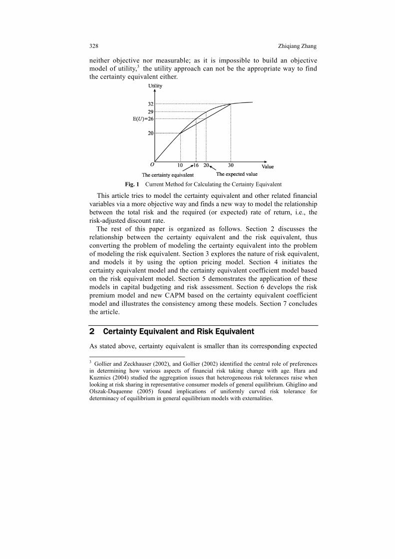
Another way to improve the NPV method is to use the certainty equivalent instead of the forecasted or expected cash flows, i.e., discount the certainty equivalents by risk-free discount rate. There are indeed (but not many) studies on the certainty equivalent, such as Hennessy and Lapan (2006), Kimball (1993), Eeckhoudt et al. (1996), Gollier and Pratt (1996), Becker and Sarin (1987), etc. However, these studies basically rely on the same assumption: the certainty equivalent of an uncertain future value is the certain value that can bring in the same expected utility without risk, as what shown in Fig. 1. By doing so, the problem of modeling the equivalent is converted into the problem of modeling the utility. Therefore, the utility function is the key for these studies. Unfortunately, the utility, as a useful economic concept, is 1 Lintner (1965) and Mossin (1966) also introduced the model independently. 2 Arbitrage pricing theory (APT) also describes the relationship between return and risk, which holds that the expected return of a financial asset can be modeled as a linear function of various macro-economic factors or theoretical market indices, where sensitivity to changes in each factor is represented by a factor-specific beta coefficient. However, as the number of factors taken into account are variable, the APT has no certain model form, thus it is less popular in academic and practical research. The theory was initiated by economist Stephen Ross in 1976.

328 Zhiqiang Zhang

neither objective nor measurable; as it is impossible to build an objective model of utility,3 the utility approach can not be the appropriate way to find the certainty equivalent either.

Fig. 1 Current Method for Calculating the Certainty Equivalent

This article tries to model the certainty equivalent and other related financial variables via a more objective way and finds a new way to model the relationship between the total risk and the required (or expected) rate of return, i.e., the risk-adjusted discount rate.

The rest of this paper is organized as follows. Section 2 discusses the relationship between the certainty equivalent and the risk equivalent, thus converting the problem of modeling the certainty equivalent into the problem of modeling the risk equivalent. Section 3 explores the nature of risk equivalent, and models it by using the option pricing model. Section 4 initiates the certainty equivalent model and the certainty equivalent coefficient model based on the risk equivalent model. Section 5 demonstrates the application of these models in capital budgeting and risk assessment. Section 6 develops the risk premium model and new CAPM based on the certainty equivalent coefficient model and illustrates the consistency among these models. Section 7 concludes the article.

2 Certainty Equivalent and Risk Equivalent

As stated above, certainty equivalent is smaller than its corresponding expected 3 Gollier and Zeckhauser (2002), and Gollier (2002) identified the central role of preferences in determining how various aspects of financial risk taking change with age. Hara and Kuzmics (2004) studied the aggregation issues that heterogeneous risk tolerances raise when looking at risk sharing in representative consumer models of general equilibrium. Ghiglino and Olszak-Duquenne (2005) found implications of uniformly curved risk tolerance for determinacy of equilibrium in general equilibrium models with externalities.

Certainty Equivalent, Risk Premium and Asset Pricing 329

value (i.e., predicted value). Here, we define the difference between the expected value and the certainty equivalent as the risk equivalent. Using X to represent the expected value, d to represent certainty equivalent coefficient, then the certainty equivalent is Xd, and: Risk equivalent = X – Xd (2) Therefore, Certainty equivalent = Xd = X – risk equivalent (3)

Equation (2) converts the problem of the certainty equivalent into the risk equivalent. In other words, the so-called certainty equivalent of a cash flow or value is its expected value minus the value reduction caused by the risk.

Therefore, the next step is naturally to scrutinize further the risk. As a general definition, risk is an uncertainty. According to the situation here, risk is the uncertainty of the forecasted cash flow or value. Of course, as an intuition or convention, risk here is mainly referred to the situation that the actual value is lower than the predicted one.

As shown in Fig. 2, X represents the expected value of the forecasted cash flow or value; S represents the possible value of the cash flow or value. Because both the abscissa (horizontal) axis and the ordinate (vertical) axis represent the identical cash flow or value, the line representing the forecasted (possible) values is the straight line x starting from the zero point and up-wards at 45 Degrees. The expected value is point E in the straight line, its scales at both abscissa and coordinate are X. Therefore, the risk is represented by the lower part of the straight line x, i.e., the part below the point E.

Fig. 2 Risk Equivalent = Guarantee Value = Put Option Value

In order to eliminate the following risk, i.e., when S is smaller than X, the straight line x does not fall below E, we need a guarantee. The guarantee

330 Zhiqiang Zhang

functions (provides value) as shown by the dashed line in Fig. 2. Therefore, comparing with the risk-free situation, the forecasted cash flow or value needs a guarantee. This implies that the certainty equivalent equals to the expected value minus the guarantee value. Or, the risk equivalent equals to the guarantee value. According to Fig. 2, just as what revealed in the extant real options research, the guarantee is a standard European put option.4 Therefore, value of the guarantee equals to the value of the corresponding put. The risk equivalent equals to the value of the put, accordingly.

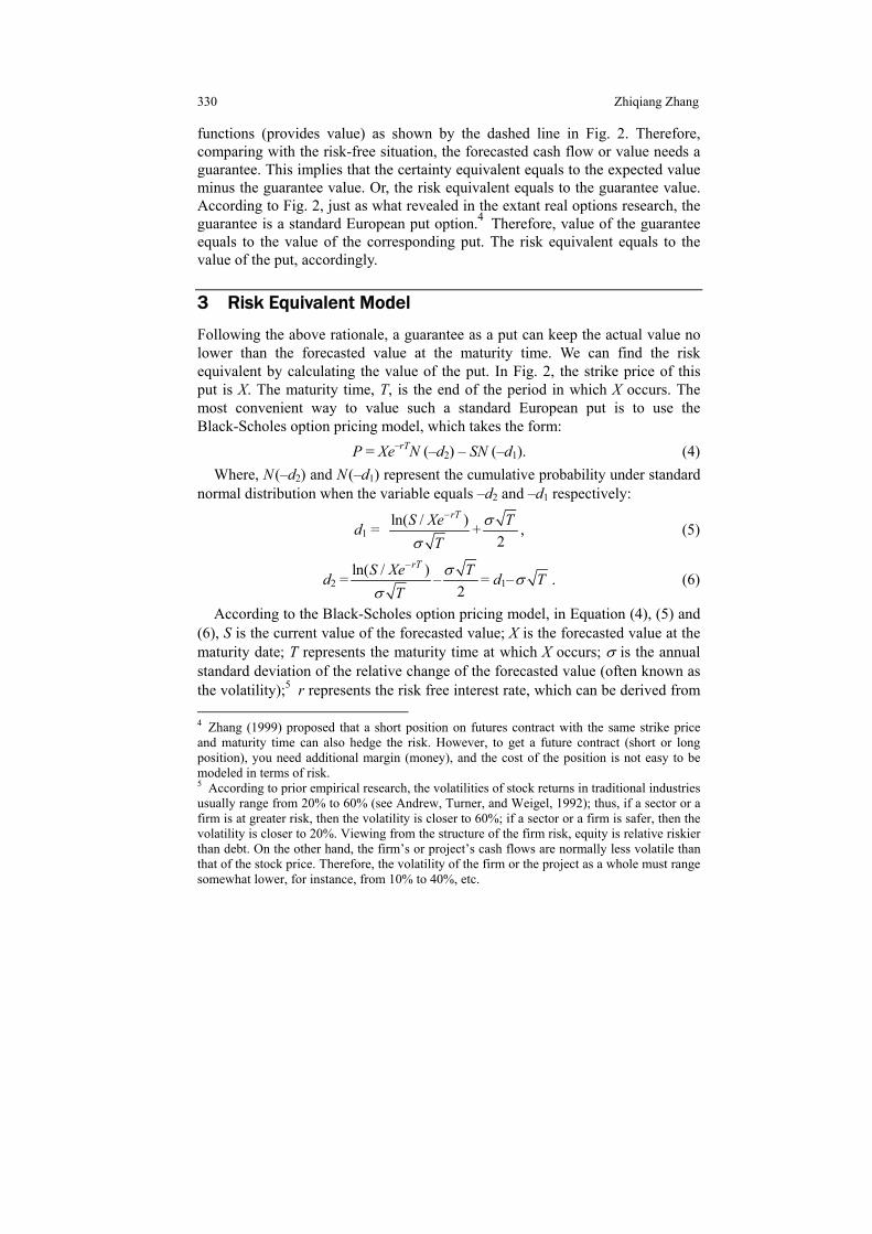
3 Risk Equivalent Model

Following the above rationale, a guarantee as a put can keep the actual value no lower than the forecasted value at the maturity time. We can find the risk equivalent by calculating the value of the put. In Fig. 2, the strike price of this put is X. The maturity time, T, is the end of the period in which X occurs. The most convenient way to value such a standard European put is to use the Black-Scholes option pricing model, which takes the form: P = Xe–rTN (–d2) – SN (–d1). (4)

Where, N (–d2) and N (–d1) represent the cumulative probability under standard normal distribution when the variable equals –d2 and –d1 respectively:

d1 = ln( / )rTS XeTσ

−

+2

Tσ , (5)

d2 =ln( / )rTS Xe

Tσ

−

–2

Tσ = d1– Tσ . (6)

According to the Black-Scholes option pricing model, in Equation (4), (5) and (6), S is the current value of the forecasted value; X is the forecasted value at the maturity date; T represents the maturity time at which X occurs; σ is the annual standard deviation of the relative change of the forecasted value (often known as the volatility);5 r represents the risk free interest rate, which can be derived from 4 Zhang (1999) proposed that a short position on futures contract with the same strike price and maturity time can also hedge the risk. However, to get a future contract (short or long position), you need additional margin (money), and the cost of the position is not easy to be modeled in terms of risk. 5 According to prior empirical research, the volatilities of stock returns in traditional industries usually range from 20% to 60% (see Andrew, Turner, and Weigel, 1992); thus, if a sector or a firm is at greater risk, then the volatility is closer to 60%; if a sector or a firm is safer, then the volatility is closer to 20%. Viewing from the structure of the firm risk, equity is relative riskier than debt. On the other hand, the firm’s or project’s cash flows are normally less volatile than that of the stock price. Therefore, the volatility of the firm or the project as a whole must range somewhat lower, for instance, from 10% to 40%, etc.

Certainty Equivalent, Risk Premium and Asset Pricing 331

the yield of the government bonds. Option pricing model usually assumes a risk neutral environment, and assumes that various values or cash flows grow or discount at the risk free interest rate in the way of continuous compounding.

The put or the guarantee is to ensure the forecasted value no less than X at time T. Therefore, the X and T in this paper are identical as that in the Black-Scholes option pricing model. The S in this paper is the present value of the relevant variable (variable X) in time T. Then S = Xe–rT and ln (S/Xe–rT) = ln (Xe–rT/Xe–rT) = 0. According to Equation (5) and (6), for the purpose of valuing the risk equivalent:

P = Xe–rT N (–d2) – SN (–d1) = Xe–rT [N (–d2) – N (–d1)] = Xe–rT [N ( / 4Tσ ) – N (– / 4Tσ )] = Xe–rT{N ( / 4Tσ ) –[1 – N ( / 4Tσ )].

Or, P = Xe–rT [2N ( / 4Tσ ) –1]. (9)

Notice that certainty equivalent and risk equivalent as well as the corresponding expected value are all occurring at the same future time T, rather than a present value. However, the value of the put derived from the Black-Scholes model is a present value. Therefore, the derived value of the put should be adjusted to its “future value” for the purpose of valuing the risk equivalent: Risk equivalent = PerT

= Xe–rT [2N ( / 4Tσ ) –1] erT = X [2N ( / 4Tσ ) –1]. (10)

Equation (10) is the model of risk equivalent.

4 Certainty Equivalent Model

Based on Equation (3) and (10), Certainty equivalent = X – Risk equivalent

= X – X [2N ( / 4Tσ ) – 1] = 2X [1 – N ( / 4Tσ ) ]. (11)

Equation (11) is the model of certainty equivalent. Accordingly, the model of certainty equivalent coefficient is:

d = 2[1 – N ( / 4Tσ )]. (12)

For convenience, we refer to Equation (12) as ZZ model of certainty equivalent coefficient, or ZZ certainty coefficient model. If we regard the certainty equivalent as corresponding to the certainty equivalent coefficient, then

332 Zhiqiang Zhang

the risk equivalent should also correspond to a coefficient. Here we define such a coefficient as risk equivalent coefficient, or risk coefficient v:

v = 1 – d = 2N( / 4Tσ ) – 1. (13)

Likewise, we refer to Equation (13) as ZZ risk coefficient model. Based on Equation (12) and (13), both the certainty equivalent coefficient and the risk coefficient depend on two factors, i.e., two common influencing factors: One is the volatility of the forecasted value, the other is the time horizon. According to Equation (12) and (13), when the σ or T equals 0, / 4Tσ = 0, N ( / 4Tσ ) = 0.5, d = 1 and v = 0; when the σ or T approaches ∞, / 4Tσ = ∞, N ( / 4Tσ ) = 1, d = 0 and v = 1. Therefore, these models illustrate that: the certainty equivalent coefficient reaches its maximum of 1 and the risk coefficient reaches its minimum of 0 under the situation of current or certain “forecasted” value; the certainty equivalent coefficient reaches its minimum value of 0 and the risk coefficient reaches its maximum value of 1 under the condition of infinite future or completely uncertain “forecasted” value; the larger of the volatility or/and the further of the time horizon, the bigger of the risk equivalent and the smaller of the certainty equivalent.

5 A Demonstration Example

For example, the initial capital investment of Project G and the following forecasted cash flows each year during the 10 years’ project life are shown in Table 1, in which the annual risk free interest rate is 5% (assumed to remain unchanged in the 10 years). Table 1 Cash Flow Forecast for Project G

Year 0 1 2 3 4 5 6 7 8 9 10

Cash flow –200 10 30 50 70 90 90 70 50 30 10

5.1 Improving the NPV Calculation If we are not concerned about potential risk, we can use the risk free rate 5% to discount the forecasted cash flows. Accordingly, the NPV of this project is:

NPV =10

1 (1 5%)t

tt

CF

= +∑ – CF0 = 384.26 – 200 = 184.26.

Now, managers of the firm want to consider risk through the certainty equivalent (or the risk equivalent). If they believe the appropriate volatility is 25%, then the ZZ certainty coefficient and the certainty equivalent are shown in

Certainty Equivalent, Risk Premium and Asset Pricing 333

Table 2.

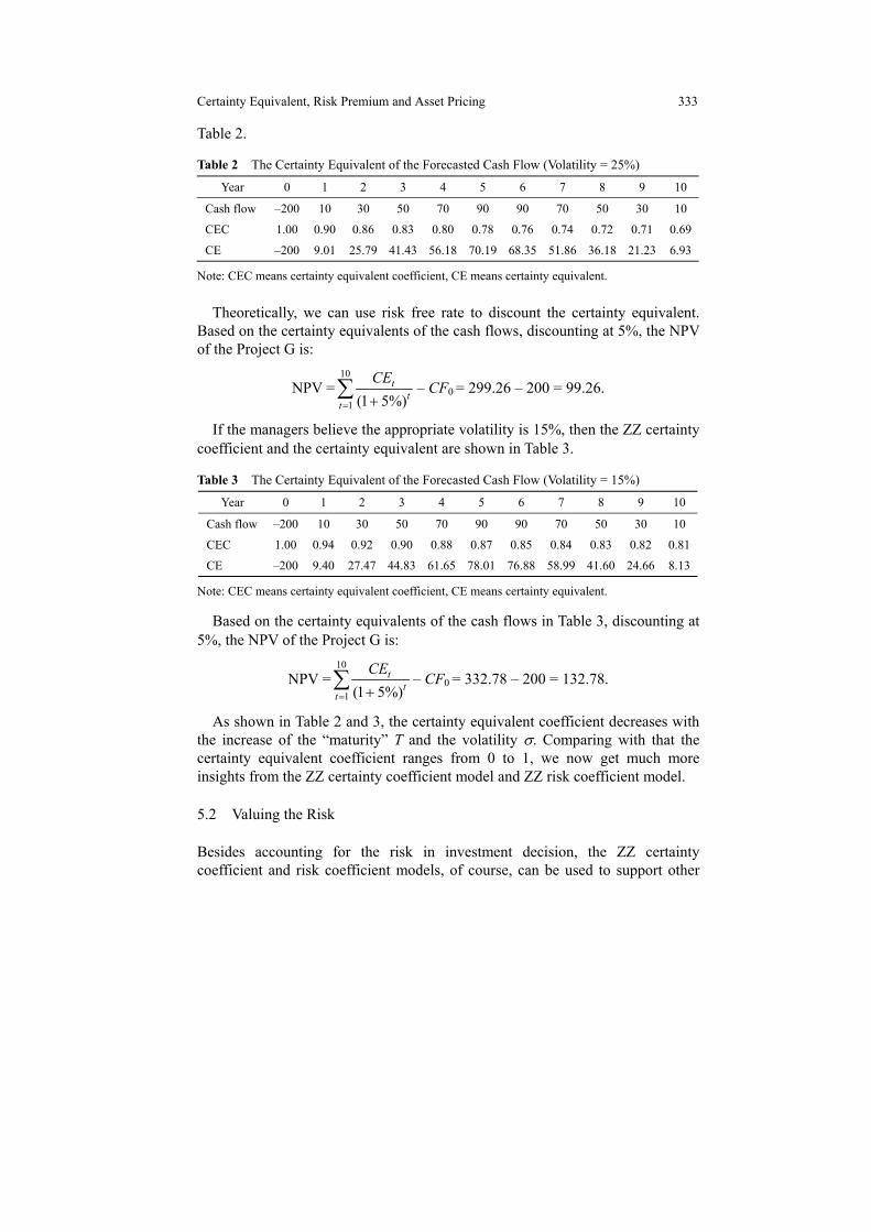
Table 2 The Certainty Equivalent of the Forecasted Cash Flow (Volatility = 25%)

Year 0 1 2 3 4 5 6 7 8 9 10

Cash flow –200 10 30 50 70 90 90 70 50 30 10

CEC 1.00 0.90 0.86 0.83 0.80 0.78 0.76 0.74 0.72 0.71 0.69

CE –200 9.01 25.79 41.43 56.18 70.19 68.35 51.86 36.18 21.23 6.93

Note: CEC means certainty equivalent coefficient, CE means certainty equivalent.

Theoretically, we can use risk free rate to discount the certainty equivalent. Based on the certainty equivalents of the cash flows, discounting at 5%, the NPV of the Project G is:

NPV =10

1 (1 5%)t

tt

CE

= +∑ – CF0 = 299.26 – 200 = 99.26.

If the managers believe the appropriate volatility is 15%, then the ZZ certainty coefficient and the certainty equivalent are shown in Table 3.

Table 3 The Certainty Equivalent of the Forecasted Cash Flow (Volatility = 15%)

Year 0 1 2 3 4 5 6 7 8 9 10

Cash flow –200 10 30 50 70 90 90 70 50 30 10

CEC 1.00 0.94 0.92 0.90 0.88 0.87 0.85 0.84 0.83 0.82 0.81

CE –200 9.40 27.47 44.83 61.65 78.01 76.88 58.99 41.60 24.66 8.13

Note: CEC means certainty equivalent coefficient, CE means certainty equivalent.

Based on the certainty equivalents of the cash flows in Table 3, discounting at 5%, the NPV of the Project G is:

NPV =10

1 (1 5%)t

tt

CE

= +∑ – CF0 = 332.78 – 200 = 132.78.

As shown in Table 2 and 3, the certainty equivalent coefficient decreases with the increase of the “maturity” T and the volatility σ. Comparing with that the certainty equivalent coefficient ranges from 0 to 1, we now get much more insights from the ZZ certainty coefficient model and ZZ risk coefficient model. 5.2 Valuing the Risk Besides accounting for the risk in investment decision, the ZZ certainty coefficient and risk coefficient models, of course, can be used to support other

334 Zhiqiang Zhang

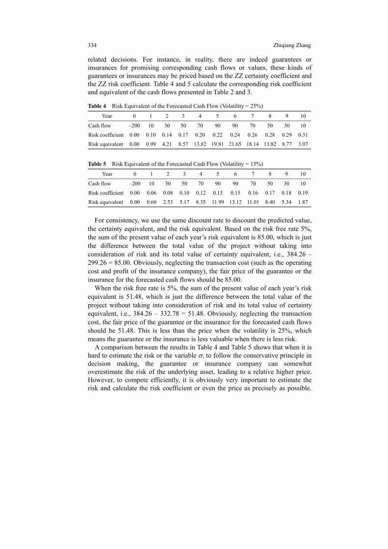
related decisions. For instance, in reality, there are indeed guarantees or insurances for promising corresponding cash flows or values, these kinds of guarantees or insurances may be priced based on the ZZ certainty coefficient and the ZZ risk coefficient. Table 4 and 5 calculate the corresponding risk coefficient and equivalent of the cash flows presented in Table 2 and 3.

Table 4 Risk Equivalent of the Forecasted Cash Flow (Volatility = 25%)

Year 0 1 2 3 4 5 6 7 8 9 10

Cash flow –200 10 30 50 70 90 90 70 50 30 10

Risk coefficient 0.00 0.10 0.14 0.17 0.20 0.22 0.24 0.26 0.28 0.29 0.31

Risk equivalent 0.00 0.99 4.21 8.57 13.82 19.81 21.65 18.14 13.82 8.77 3.07

Table 5 Risk Equivalent of the Forecasted Cash Flow (Volatility = 15%)

Year 0 1 2 3 4 5 6 7 8 9 10

Cash flow –200 10 30 50 70 90 90 70 50 30 10

Risk coefficient 0.00 0.06 0.08 0.10 0.12 0.13 0.15 0.16 0.17 0.18 0.19

Risk equivalent 0.00 0.60 2.53 5.17 8.35 11.99 13.12 11.01 8.40 5.34 1.87

For consistency, we use the same discount rate to discount the predicted value,

the certainty equivalent, and the risk equivalent. Based on the risk free rate 5%, the sum of the present value of each year’s risk equivalent is 85.00, which is just the difference between the total value of the project without taking into consideration of risk and its total value of certainty equivalent, i.e., 384.26 – 299.26 = 85.00. Obviously, neglecting the transaction cost (such as the operating cost and profit of the insurance company), the fair price of the guarantee or the insurance for the forecasted cash flows should be 85.00.

When the risk free rate is 5%, the sum of the present value of each year’s risk equivalent is 51.48, which is just the difference between the total value of the project without taking into consideration of risk and its total value of certainty equivalent, i.e., 384.26 – 332.78 = 51.48. Obviously, neglecting the transaction cost, the fair price of the guarantee or the insurance for the forecasted cash flows should be 51.48. This is less than the price when the volatility is 25%, which means the guarantee or the insurance is less valuable when there is less risk.

A comparison between the results in Table 4 and Table 5 shows that when it is hard to estimate the risk or the variable σ, to follow the conservative principle in decision making, the guarantee or insurance company can somewhat overestimate the risk of the underlying asset, leading to a relative higher price. However, to compete efficiently, it is obviously very important to estimate the risk and calculate the risk coefficient or even the price as precisely as possible.

Certainty Equivalent, Risk Premium and Asset Pricing 335

Of course, it is equally important to know the precise risk coefficient and the price of the guarantee or the insurance for the guaranteed or the insured firms.

Furthermore, discovering a new and effective pricing method can play a role far more important than what has been illustrated in the above example, i.e., set a standard or guidance for pricing. For the guarantee or insurance firms or other risk-related financial firms, the new and more effective pricing method may be a necessary precondition for new business development as pricing is an essential step for new business. As to financial products, such as the insurance or guarantee, pricing model or method is a must for the practical pricing. As empirical pricing model is seriously lacking, the invention of new theoretical pricing model determines the feasibility of the new financial business, to some extent. The celebrated Black-Scholes model and its applications have been a key ingredient to the booming of various financial derivatives in the past decades.

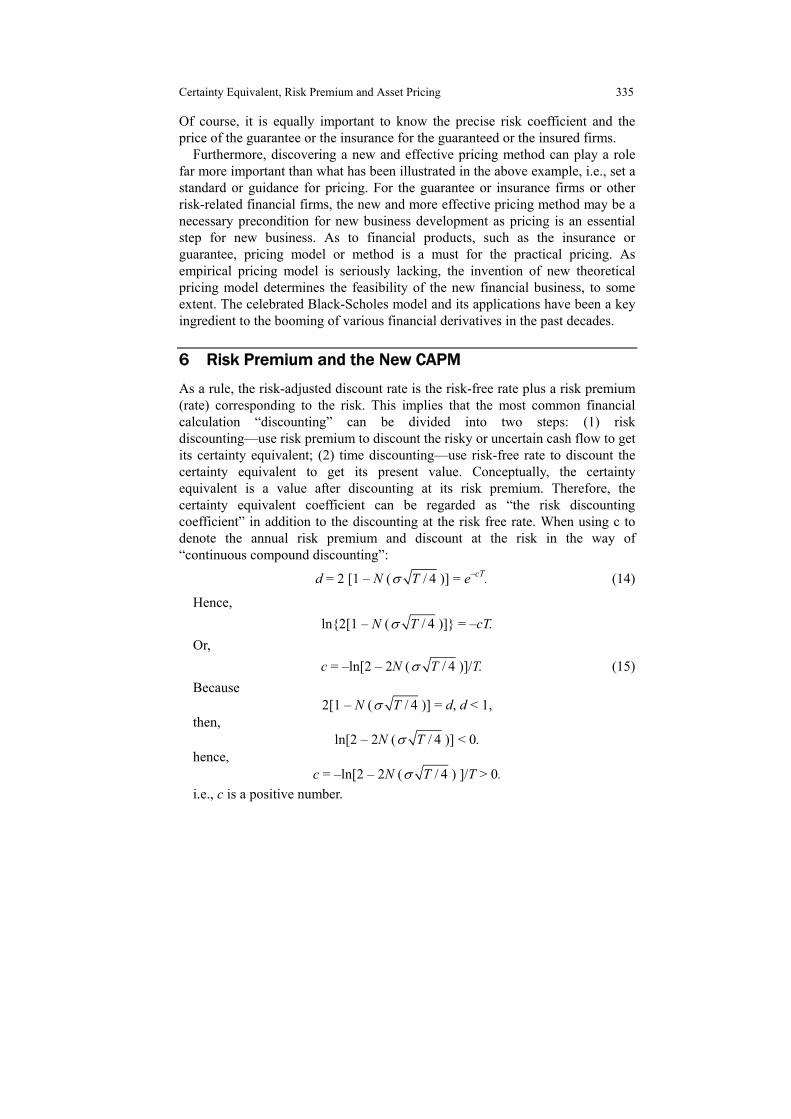
6 Risk Premium and the New CAPM

As a rule, the risk-adjusted discount rate is the risk-free rate plus a risk premium (rate) corresponding to the risk. This implies that the most common financial calculation “discounting” can be divided into two steps: (1) risk discounting—use risk premium to discount the risky or uncertain cash flow to get its certainty equivalent; (2) time discounting—use risk-free rate to discount the certainty equivalent to get its present value. Conceptually, the certainty equivalent is a value after discounting at its risk premium. Therefore, the certainty equivalent coefficient can be regarded as “the risk discounting coefficient” in addition to the discounting at the risk free rate. When using c to denote the annual risk premium and discount at the risk in the way of “continuous compound discounting”:

d = 2 [1 – N ( / 4Tσ )] = e–cT. (14)

Hence, ln{2[1 – N ( / 4Tσ )]} = –cT.

Or, c = –ln[2 – 2N ( / 4Tσ )]/T. (15)

Because 2[1 – N ( / 4Tσ )] = d, d < 1,

then, ln[2 – 2N ( / 4Tσ )] < 0.

hence, c = –ln[2 – 2N ( / 4Tσ ) ]/T > 0.

i.e., c is a positive number.

336 Zhiqiang Zhang

Using k to represent the risk adjusted discount rate, and r the risk free rate, then: k = r + c = r – ln{2[1 – N ( / 4Tσ )]}/T. (16)

Obviously, as a rate of return or cost of capital, k in Equation (16) accounts for the total risk. To maintain consistency, Equation (15) is referred to as the ZZ risk premium model and Equation (16) the ZZ risk-adjusted discount rate model or the ZZ capital asset pricing model or ZZ CAPM.

ZZ CAPM, different from Sharpe’s CAPM, accounts for not only the systematic risk but also the non-systematic risk. Another difference worthy mentioning is that ZZ CAPM accounts for the effect of diversification among periods, while Sharpe’s CAPM only accounts for the effect of perfect diversification among all securities or infinite securities. Thus the ZZ CAPM reveals explicitly an almost forgotten principle: regarding an investment in a security, the longer the holding period, the lower the risk. Hence, the successful experience from long-term investment (such as Warren E. Buffett) can be explained. Therefore, the ZZ CAPM implies that the risk premium and the risk-adjusted discount rate decrease with the increase of the number of the investment (holding) periods.

Again in the previous example in Section 5, when the volatility level is 15% and 25% respectively, the corresponding c and k are calculated based on the ZZ risk premium model and the ZZ CAPM as shown in Table 6 and 7 respectively.

Table 6 Estimation of Risk Adjusted Discount Rate k (Volatility = 15%)

Year 1 2 3 4 5 6 7 8 9 10

c 0.062 0.044 0.036 0.032 0.029 0.026 0.024 0.023 0.022 0.021

d 0.940 0.916 0.897 0.881 0.867 0.854 0.843 0.832 0.822 0.813

k 0.112 0.094 0.086 0.082 0.079 0.076 0.074 0.073 0.072 0.071

e–kT 0.894 0.828 0.772 0.721 0.675 0.633 0.594 0.558 0.524 0.493

Note: e–kT is the coefficient of present value taking into consideration both the systematic and non-systematic risk, and e–kT = e–(r + c)T = e–rTe–cT, means that the discounting can be divided into two steps: risk discounting and time discounting.

In Table 6 and 7, the c, or the annual risk premium rate as well as the risk-adjusted discount rate, decreases with the extension of the due time. As explained above, this is because the investment is better diversified with the increase of the periods and more risks are eliminated in longer periods. Nevertheless, the certainty equivalent coefficient still keeps decreasing progressively year by year. Similarly, the total coefficient of present value, e–kT, calculated based on the total discount rate k, also keeps decreasing progressively year by year. This implies that as time goes by, the larger part of its value is

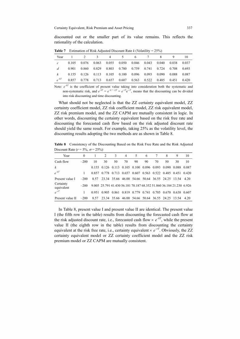
Certainty Equivalent, Risk Premium and Asset Pricing 337

discounted out or the smaller part of its value remains. This reflects the rationality of the calculation.

Table 7 Estimation of Risk Adjusted Discount Rate k (Volatility = 25%)

Year 1 2 3 4 5 6 7 8 9 10

c 0.105 0.076 0.063 0.055 0.050 0.046 0.043 0.040 0.038 0.037

d 0.901 0.860 0.829 0.803 0.780 0.759 0.741 0.724 0.708 0.693

k 0.155 0.126 0.113 0.105 0.100 0.096 0.093 0.090 0.088 0.087

e–kT 0.857 0.778 0.713 0.657 0.607 0.563 0.522 0.485 0.451 0.420

Note: e–kT is the coefficient of present value taking into consideration both the systematic and non-systematic risk, and e–kT = e–(r + c)T = e–rTe–cT, means that the discounting can be divided into risk discounting and time discounting.

What should not be neglected is that the ZZ certainty equivalent model, ZZ certainty coefficient model, ZZ risk coefficient model, ZZ risk equivalent model, ZZ risk premium model, and the ZZ CAPM are mutually consistent in logic. In other words, discounting the certainty equivalent based on the risk free rate and discounting the forecasted cash flow based on the risk adjusted discount rate should yield the same result. For example, taking 25% as the volatility level, the discounting results adopting the two methods are as shown in Table 8. Table 8 Consistency of the Discounting Based on the Risk Free Rate and the Risk Adjusted Discount Rate (r = 5%, σ = 25%)

Year 0 1 2 3 4 5 6 7 8 9 10

Cash flow –200 10 30 50 70 90 90 70 50 30 10

k 0.155 0.126 0.113 0.105 0.100 0.096 0.093 0.090 0.088 0.087

e–kT 1 0.857 0.778 0.713 0.657 0.607 0.563 0.522 0.485 0.451 0.420

Present value I –200 8.57 23.34 35.66 46.00 54.66 50.64 36.55 24.25 13.54 4.20 Certainty equivalent –200 9.005 25.791 41.430 56.181 70.187 68.352 51.860 36.184 21.230 6.926

e–rT 1 0.951 0.905 0.861 0.819 0.779 0.741 0.705 0.670 0.638 0.607

Present value II –200 8.57 23.34 35.66 46.00 54.66 50.64 36.55 24.25 13.54 4.20

In Table 8, present value I and present value II are identical. The present value

I (the fifth row in the table) results from discounting the forecasted cash flow at the risk adjusted discount rate, i.e., forecasted cash flow × e–kT, while the present value II (the eighth row in the table) results from discounting the certainty equivalent at the risk free rate, i.e., certainty equivalent × e–rT. Obviously, the ZZ certainty equivalent model or ZZ certainty coefficient model and the ZZ risk premium model or ZZ CAPM are mutually consistent.

338 Zhiqiang Zhang

7 Conclusion

It has become an accepted practice that the certainty equivalent, the certainty equivalent coefficient as well as the risk adjusted discount rate are all estimated via the subjective or experience-based method. To propose a more objective and empirical approach, this article establishes the ZZ certainty equivalent model, ZZ certainty coefficient model, ZZ risk coefficient model, ZZ risk equivalent model, ZZ risk premium model and ZZ CAPM. These models are mutually consistent in logic and capable of completing the related financial calculations, such as the estimation of the risk and equivalent, valuation of risk and NPV of an investment, understanding of the relationship between risk and return, and estimation of the risk-adjusted discount rate or required rate of return on an investment, etc. They are both sound in theory and feasible in practice, which can be used to assist managers in making financial decisions, as well as to improve related financial analysis, appraisal, and management.

References

Becker J L, Sarin R K (1987). Lottery dependent utility. Management Science, 33: 1367–1382 Diamond P, Stiglitz J E (1974). Increases in risk and in risk aversion. Journal of Economic

Theory, 8: 337–360 Fama E (1977). Risk-adjusted discount rates and capital budgeting under uncertainty. Journal

of Financial Economics, 5(1): 3–24 Gollier C (2002a). Discounting an uncertain future. Journal of Public Economics, 85:

149–166 Gollier C (2002b). Time diversification, liquidity constraints, and decreasing aversion to risk

on wealth. Journal of Monetary Economics, 49(8): 1439–1459 Gollier C (2002c). Time horizon and the discount rate. Journal of Economic Theory, 107(3):

463–473 Gollier C, Pratt J W (1996). Risk vulnerability and the tempering effect of background risk.

Econometrica, 64(6): 1109–1123 Gollier C, Zeckhauser R J (2002). Horizon length and portfolio risk. Journal of Risk and

Uncertainty, 24(4): 195–212 Gordon A S (1986). A certainty-equivalent approach to capital budgeting. Financial

Management, 15(4): 23–32 Gray D F, Merton R C, Bodie Z (2007). Contingent claims approach to measuring and

managing sovereign credit risk. Journal of Investment Management, 5(4): 5–28 Grinblatt M, Titman S (1998). Financial Markets and Corporate Strategy, Chapter 10.

McGraw-Hill Inc. Groom B, Koundouri P, Panopoulou E, Pantelidis T (2004). Model selection for estimating

certainty equivalent discount rates. Working paper, University College London, London, UK Hong C S, Herk L F (1996). Increasing risk aversion and diversification preference. Journal of

Economic Theory, 70(2): 180–200 Kimball M S (1993). Standard risk aversion. Econometrica, 61(4): 589–611

Certainty Equivalent, Risk Premium and Asset Pricing 339

Machina M J (1987). Choice under uncertainty: Problems solved and unsolved. Economic Perspectives, 1: 121–154

Merton R C (2000). Future possibilities in finance theory and finance practice. Working paper, Harvard Business School

Myers S C, Turbull S M (1977). Capital budgeting and the capital asset pricing model: Good news and bad news. Journal of Finance, 32(2): 321–333

Ogaki M, Zhang Q (2001). Decreasing relative risk aversion and tests of risk sharing. Econometrica, 69(3): 515–526

Pearce D, Groom B, Hepburn C, Koundouri P (2003). Valuing the future: Recent advances in social discounting. World Economics, 4(3): 121–141

Rabin M (2000). Risk aversion and expected-utility theory: A calibration theorem. Econometrica, 68(6): 1281–1292

Robichek A A, Myers S C (1966). Conceptual problems in the use of risk-adjusted discount rates. Journal of Finance, 21(1): 727–730

Samuelson A (1967). General proof that diversification pays. Journal of Financial and Quantitative Analysis, 2(2): 1–13

Schmalensee R (1981). Risk and return on long-lived tangible assets. Journal of Financial Economics, 2(2): 185–205

Trippi R R (1989). A discount rate adjustment for calculation of expected net present values and internal rates of return of investments whose lives are uncertain. Journal of Economics and Business, 41(2): 143–151

Turner A L, Weigel E J (1992). Daily stock market volatility: 1928–1989. Management Science, 38(11): 1586–1609

Weitzman M (1998). Why the far distant future should be discounted at its lowest possible rate. Journal of Environmental Economics and Management, 36: 201–208

Weitzman M (2001). Gamma discounting. American Economic Review, 91(1): 261–271 Zhang Z (2009). Determine optimal capital structure based on revised definitions of tax shield

and bankruptcy cost. Frontiers of Business Research in China, 3(1): 120–144