Analysis of Adaptive Certainty-Equivalent … of Adaptive Certainty-Equivalent Techniques for ... in...

eeh power systemslaboratory

Jose Sebastian Espejo-Uribe

Analysis of Adaptive Certainty-EquivalentTechniques for the Stochastic Unit

Commitment Problem

Master ThesisPSL1707

EEH – Power Systems LaboratorySwiss Federal Institute of Technology (ETH) Zurich

Examiner: Prof. Dr. Gabriela HugSupervisor: Dr. Tomas Tinoco De Rubira

Zurich, April 21, 2017

Abstract

The unit commitment problem aims to schedule the most cost-effective com-bination of generating units to meet the demand while taking into accounttechnical and operational constraints. With the projected large-scale pene-tration of renewable energy sources, in particular wind and solar, which arehighly variable and intermittent, uncertainty must be properly considered.In this thesis, the applicability and performance of the Adaptive Certainty-Equivalent algorithm for solving the stochastic unit commitment problemwith large penetration of renewable energy is studied. This approach hasbeen previously applied to the stochastic economic dispatch problem withpromising results, but the presence of binary restrictions in the stochasticunit commitment problem pose both practical and theoretical challengesthat warrant investigation. It is shown in this work that despite a lackof theoretical guarantees, the Adaptive Certainty-Equivalent algorithm canfind commitment schedules in reasonable times that are better than thoseobtained with benchmark algorithms.

i

Contents

List of Acronyms iii

List of Symbols iv

1 Introduction 1

2 Stochastic Unit Commitment Problem 42.1 Problem Formulation . . . . . . . . . . . . . . . . . . . . . . . 42.2 Model of Uncertainty . . . . . . . . . . . . . . . . . . . . . . . 6

3 Sample-Average Approximation 83.1 Benders Decomposition . . . . . . . . . . . . . . . . . . . . . 8

4 Stochastic Hybrid Approximation 104.1 Adaptive Certainty-Equivalent . . . . . . . . . . . . . . . . . 114.2 Applicability to Stochastic Unit Commitment . . . . . . . . . 114.3 Noise Reduction . . . . . . . . . . . . . . . . . . . . . . . . . 14

5 Numerical Experiments 165.1 Implementation . . . . . . . . . . . . . . . . . . . . . . . . . . 165.2 Test Cases . . . . . . . . . . . . . . . . . . . . . . . . . . . . . 175.3 Renewables . . . . . . . . . . . . . . . . . . . . . . . . . . . . 185.4 Benders Validation . . . . . . . . . . . . . . . . . . . . . . . . 205.5 Performance and Solutions . . . . . . . . . . . . . . . . . . . . 20

5.5.1 Case A . . . . . . . . . . . . . . . . . . . . . . . . . . 215.5.2 Case B . . . . . . . . . . . . . . . . . . . . . . . . . . 225.5.3 Case C . . . . . . . . . . . . . . . . . . . . . . . . . . 23

6 Conclusions 27

Bibliography 29

ii

List of Acronyms

AdaCE Adaptive Certainty-Equivalent

CE Certainty-Equivalent

ED Economic Dispatch

LP Linear Program

MILP Mixed-Integer Linear Programming

MIQP Mixed-Integer Quadratic Programming

MINLP Mixed-Integer Non-Linear Programming

MISO Midcontinent Independent System Operator

NR Noise Reduction

SAA Sample-Average Approximation

SHA Stochastic Hybrid Approximation

UC Unit Commitment

iii

List of Symbols

Latin Letters

ak Constant term of under estimator at iteration k

A Sparse matrix

bk Linear term of under estimator at iteration k

cdi Shut-down cost of generator i

cui Start-up cost of generator i

d Vector of supplied load powers

d Vector of requested load powers

D Sparse matrix

E [ · ] Expectation with respect to w

F First stage start-up and shut-down cost function

J Sparse matrix

k Algorithm iterations

L Sparse matrix

m Number of realizations drawn of renewable power vectors

n Number of conventional generation units

nr Number of renewable sources

N Node distance parameter

p Vector of generator output powers

pi,t Output power of generator i during time t

pmax Vector of maximum generator power limits

pmin Vector of minimum generator power limits

P Sparse matrix

Q Recourse function that quantifies total operating cost

iv

CONTENTS v

Q Recourse function with piece-wise linear generating costs

Q0 Initial function approximation

Qk Function approximation at iteration k

r Number of linear segments

s Vector of utilized powers from renewable sources

S Sparse matrix

T Time horizon

T ui Minimum up time for generator i

T di Minimum down time for generator i

u Vector of on-off states of generators

ui,0 Initial on-off state of generator i

ui,t On-off state of generator i during time t

uk Candidate solution at iteration k

U Set of minimum up and down time restrictions

w Vector of powers from renewable energy sources

wmax Vector of power capacities of renewable energy sources

wk Sample of random vector w drawn at iteration k

wk,i One of many samples of random vector w drawn at iteration k

wt Vector of non-negative base powers

x Second-stage cost epigraph auxiliary variable

yi,t Start-up cost epigraph auxiliary variable

zi,t Shut-down cost epigraph auxiliary variable

zmax Vector of maximum branch flow limits

zmin Vector of minimum branch flow limits

Greek Letters

αk Step length at iteration k

βi,j Constant of piecewise linear approximation

γ Load not serve cost

δmax Vector of maximum generator ramping limits

δmin Vector of minimum generator ramping limits

CONTENTS vi

ζi,j Constant of piecewise linear approximation

θ Vector of bus voltage angles

µ Expectation of noisy subgradient

µki Lagrange multiplier

ξk Noisy subgradient of recourse function at iteration k

ξk,i One of many noisy subgradients of recourse function at iteration k

πki Lagrange multiplier

Πc Projection operator

ρ Correlation coefficient parameter

Σ Covariance of noisy subgradient

Σm Covariance of averaged noisy subgradients

Σt Covariance of renewable powers

Σt Positive semidefinite matrix

ϕ Generation cost function

ϕ Piece-wise linear generation cost function

Chapter 1

Introduction

The Unit Commitment (UC) problem aims to schedule the most cost-effectivecombination of generating units to meet the demand while taking into ac-count technical and operational constraints [1]. Due to strong temporal limi-tations of some units, e.g., long start-up times, the schedule must be plannedin advance. Usually, this is done the day before for a time horizon of 24 hourswith hourly resolution. Due to its non-convexity and scale, the UC problemposes serious computational challenges, especially since the time availableto solve it is limited in practice [2]. For example, the Midcontinent Indepen-dent System Operator (MISO) needs to solve a UC problem with around1400 generating units in about 20 minutes [3]. Until recently, uncertaintycame mainly from demand variations and potential fault occurrences, wasrelatively low, and hence deterministic UC models were acceptable. How-ever, with the projected large-scale penetration of renewable energy sources,in particular wind and solar, which are highly variable and intermittent, un-certainty must be properly considered. If not, operating costs of the systemcould become excessively high and also security issues could arise [4] [5].For this reason, algorithms that can solve UC problems with high levels ofuncertainty efficiently are highly desirable.

For the past 40 years, there has been extensive research by the scien-tific community on the UC problem. In particular, research has focusedon analyzing the practical issues and economic impacts of UC in verticallyintegrated utilities and in deregulated markets, and on leveraging advancesin optimization algorithms. With regards to algorithms, the most exploredapproaches have been based on the following: dynamic programming [6],Mixed-Integer Linear Programming (MILP) [7] [8], and heuristics [9]. Ap-proaches for dealing with uncertainty in UC have been mostly based onrobust optimization [10], chance-constrained optimization [11], and stochas-tic optimization. Those based on the latter have typically used scenarios,or Sample-Average Approximations (SAA), combined with Benders decom-position [12] or with Lagrangian relaxation [13]. For example, in [8], the

1

CHAPTER 1. INTRODUCTION 2

authors explore the benefits of stochastic optimization over a deterministicapproach for solving a UC problem with large amounts of wind power. Un-certainty is represented with a scenario tree and the resulting problem issolved directly using an MILP solver. The authors in [12] also use scenariosto model wind uncertainty in UC but use Benders decomposition to exploitthe structure of the resulting two-stage problem combined with heuristics toimprove its performance. In [14], the authors use Lagrangian relaxation todecompose a multi-stage stochastic UC problem into single-scenario prob-lems and exploit parallel computing resources. For more information onapproaches for solving the UC problem, the interested reader is referred to[2].

Stochastic Hybrid Approximation (SHA) algorithms are a family of al-gorithms for solving stochastic optimization problems. They were initiallyproposed in [15] and are characterized by working directly with stochas-tic quantities at every iteration, and using these to improve deterministicmodels of expected-value functions. They have the key property that theycan leverage accurate initial approximations of expected-value functions pro-vided by the user, and that the improvements to these functions made duringthe execution of the algorithm do not change their structure. Algorithms ofthis type have been recently applied to stochastic Economic Dispatch (ED)problems, which are closely related to the stochastic UC problem but focusexclusively on determining generator power levels and not on-off states. Inparticular, in [16], the authors apply the SHA algorithm proposed in [15]to a two-stage stochastic ED problem by using a certainty-equivalent modelfor constructing the initial approximation of the expected second-stage cost.The resulting “Adaptive Certainty-Equivalent” (AdaCE) approach is shownto have superior performance compared to some widely-used approacheson the test cases considered. The same authors also later extend this ap-proach to solve more complex versions of the stochastic ED problem thatinclude expected-value constraints and multiple planning stages [17] [18],and show promising performance. The close connection between UC andED problems suggests that perhaps the combination of SHA and certainty-equivalent models may also lead to a promising approach for solving stochas-tic UC problems. However, the theoretical and practical issues that couldarise due to the binary variables present in the UC problem warrant furtherinvestigation in order to validate this hypothesis.

In this thesis, the applicability and performance of the AdaCE algo-rithm, which combines SHA with initial expected-value function approxi-mations based on certainty-equivalent models, is studied. More specifically,the stochastic UC problem is formulated as a two-stage mixed-integer opti-mization problem that captures the essential properties of the problem thatmake it challenging to solve, namely, binary variables, causality, and uncer-tainty. The theoretical and practical challenges associated with the use ofthe AdaCE algorithm for solving this problem are explored. In particular,

CHAPTER 1. INTRODUCTION 3

possible outcomes and practical limitations on the types of approximationsare investigated. Additionally, ideas inspired from the mini-batch techniqueused in Machine Learning are considered for improving the performance ofthe algorithm on this problem. Furthermore, the performance of the algo-rithm is compared against that of a deterministic approach and that of thewidely-used SAA or scenario approach combined with Benders decomposi-tion on test cases constructed from several power networks and renewableenergy distributions. The results obtained show that despite a lack of theo-retical guarantees, the AdaCE algorithm can find commitment schedules inreasonable times that are better than the ones obtained with the benchmarkalgorithms considered.

This thesis is organized as follows: In Chapter 2, the two-stage mixed-integer model of the stochastic UC problem used in this work is presented.In Chapter 3, a benchmark algorithm based on SAA and Benders decom-position is described. In Chapter 4, the AdaCE algorithm is introduced,and potential theoretical and practical issues and solutions are discussed.In Chapter 5, the experiments performed to compare the performance ofthe algorithms described in this work are presented and the results obtainedare discussed. Lastly, in Chapter 6, key findings are summarized and nextresearch directions are outlined.

Chapter 2

Stochastic Unit CommitmentProblem

As already mentioned, the stochastic UC problem consists of determiningthe most cost-effective schedule of power generating units to meet the de-mand while taking into account device limits, operational constraints, anduncertainty. Typically, the scheduling period of interest is 24 hours with aresolution of one hour. In a vertically integrated utility, the schedule de-fines periods of time during which each generating unit will be on or off,respecting its minimum up and down times. Power production levels aretypically determined shortly before delivery in a process known as ED, andare therefore not part of the unit commitment schedule. On the other hand,in a deregulated electricity market, both on-off states and power productionlevels are determined jointly during market clearing [19]. The schedules arechosen to maximize profit or social welfare, and special attention is paid toenergy pricing and payments [20]. Traditionally, the uncertainty in a systemhas been small and it has come mainly from the demand and potential con-tingencies. However, with the projected large-scale penetration of renewableenergy in power systems, in particular of wind and solar, the uncertainty isexpected to be quite high, and hence a proper treatment of this is crucial forensuring system reliability and economic efficiency in next-generation powersystems.

2.1 Problem Formulation

In this thesis, the stochastic UC problem is modeled as a stochastic two-stage mixed-integer optimization problem. This model, albeit simplified,allows capturing the following key properties that make this problem com-putationally challenging:

• The commitment decisions are restricted to be either on or off, i.e.,they are binary.

4

CHAPTER 2. STOCHASTIC UNIT COMMITMENT PROBLEM 5

• The commitment schedule needs to be determined ahead of operation.

• The commitment schedule needs to respect the inter-temporal con-straints of the generating units.

• The operation of the system is strongly affected by the availability ofrenewable energy, which is highly uncertain.

• Network security constraints can impose restrictions on the utilizationof the available generation resources.

Hence, it serves as an adequate model for performing an initial assessment ofthe applicability and performance of an algorithm for solving the stochasticUC problem.

Mathematically, the problem is given by

minimizeu

F (u) + E [Q(u,w)] (2.1)

subject to u ∈ U ∩ {0, 1}nT ,

where u is the vector of on-off states ui,t for each power generating uniti ∈ {1, . . . , n} and time t ∈ {1, . . . , T}, w is the vector of random powersfrom renewable energy sources during the operation period, and E [ · ] denotesexpectation with respect to w. The function F is an LP-representable costfunction, i.e., it can be represented as a linear program. It is given by

F (u) =n∑i=1

T∑t=1

(cui max{ui,t − ui,t−1, 0}+ cdi max{ui,t−1 − ui,t, 0}

),

for all u ∈ {0, 1}nT , where cui and cdi are the start-up and shut-down costsfor generator i, respectively, and ui,0 ∈ {0, 1} are known constants. Theconstraint u ∈ U represents the minimum up and down time restrictions ofthe generating units, which serve to prevent the erosion caused by frequentchanges of thermal stress. They are given by

ui,t − ui,t−1 ≤ ui,τ , ∀i ∈ {1, . . . , n},∀(t, τ) ∈ Suiui,t−1 − ui,t ≤ 1− ui,τ , ∀i ∈ {1, . . . , n},∀(t, τ) ∈ Sdi ,

where

Sui :={

(t, τ)∣∣∣ t ∈ {1, . . . , T

}, τ ∈

{t+ 1, . . . ,min{t+ T ui − 1, T}

}}Sdi :=

{(t, τ)

∣∣∣ t ∈ {1, . . . , T}, τ ∈

{t+ 1, . . . ,min{t+ T di − 1, T}

}},

and T ui and T di are the minimum up and down times for unit i, respectively.The “recourse” function Q(u,w) quantifies the operation cost of the sys-

tem for a given commitment schedule u of generating units and available


powers w from renewable energy sources. It is modeled as the optimal ob-jective value of the following multi-period DC Optimal Power Flow (OPF)problem:

minimizep,θ,s,d

ϕ(p) + γ∥∥d− d∥∥

1(2.2a)

subject to Pp+ Ss− Ld−Aθ = 0 (2.2b)

diag(pmin)u ≤ p ≤ diag(pmax)u (2.2c)

δmin ≤ Dp ≤ δmax (2.2d)

zmin ≤ Jθ ≤ zmax (2.2e)

0 ≤ d ≤ d (2.2f)

0 ≤ s ≤ w, (2.2g)

where p are generator powers, s are the utilized powers from renewableenergy sources, d and d are the requested and supplied load powers, re-spectively, and θ are bus voltage angles during the operation period. Thefunction ϕ is a separable convex quadratic function that quantifies the gen-eration cost, and γ‖d − d‖1 quantities the cost of load not served (γ ≥ 0).Constraint (2.2b) enforces power flow balance using a DC network model[21], constraint (2.2c) enforces generator power limits, constraint (2.2d) en-forces generator ramping limits, constraint (2.2e) enforces branch flow limitsdue to thermal ratings, and constraints (2.2g) and (2.2f) impose limits onthe utilized renewable powers and on the supplied load. Lastly, P , S, L,A, D, J are sparse matrices. It can be shown that the function Q( · , w) isconvex for all w [22].

It is assumed for simplicity that the second-stage problem (2.2) is feasiblefor all u ∈ U∩{0, 1}nT and almost all w. This property is commonly referredto as relatively complete recourse, and guarantees that E [Q(u,w)] < ∞ forall u ∈ U ∩ {0, 1}nT . Typically, allowing emergency load curtailment, as inproblem (2.2), or other sources of flexibility such as demand response, areenough to ensure this property in practical problems.

2.2 Model of Uncertainty

The vector of available powers from renewable energy sources for each timet ∈ {1, . . . , T} is modeled by

wt := Πc(wt + δt),

where wt is a vector of non-negative “base” powers and δt ∼ N (0,Σt). Πc isthe projection operator given by

Πc(z) := arg min{‖z − w‖2

∣∣ 0 ≤ w ≤ wmax}, ∀z,


where wmax is the vector of power capacities of the renewable energy sources.The random vector w in (2.1) is therefore composed of (w1, . . . , wT ). Thecovariance matrix Σt is assumed to be given by Σt := (t/T )Σt, where Σt

is a positive semidefinite matrix whose diagonal is equal to the element-wise square of wt, and off-diagonals are such that the correlation coefficientbetween powers of sources at most N branches away equals some pre-definedρ and zero otherwise. With this model, the forecast uncertainty increaseswith time and with base power levels.

Chapter 3

Sample-AverageApproximation

Since evaluating the function E [Q( · , w)] in (2.1) accurately is computation-ally expensive, algorithms for solving problems of the form of (2.1) resortto approximations. A widely used approximation consists of the sample av-erage m−1

∑mi=1Q( · , wi), where m ∈ Z++ and wi are realizations of the

random vector w, which are often called scenarios. Hence, this approach istypically referred to as sample-average approximation or scenario approach[23]. The resulting approximate problem is given by

minimizeu

F (u) +1

m

m∑i=1

Q(u,wi) (3.1)

subject to u ∈ U ∩ {0, 1}nT ,

which is a deterministic optimization problem. It can be shown that bymaking m sufficiently large, the solutions of problem (3.1) approach thoseof problem (2.1) [23]. However, as m increases, problem (3.1) becomes verydifficult to solve due to its size. For this reason it becomes necessary toexploit the particular structure of this problem.

3.1 Benders Decomposition

A widely used strategy for dealing with the complexity of problem (3.1)is to use decomposition combined with a cutting-plane method [22]. Thisapproach, which is known as Benders decomposition, replaces the sample-average function m−1

∑mi=1Q( · , wi) with a gradually-improving piece-wise

linear approximation. The “pieces” of this piece-wise linear approximationare constructed from values and subgradients of the sample-average function,and these can be computed efficiently using parallel computing resources[22].

8

CHAPTER 3. SAMPLE-AVERAGE APPROXIMATION 9

More specifically, the algorithm performs the following steps at eachiteration k ∈ Z+:

uk = arg min{F (u) +Qk(u)

∣∣∣ u ∈ U ∩ {0, 1}nT } (3.2a)

Qk+1(u) =

{ak + bTk (u− uk) if k = 0,max

{Qk(u), ak + bTk (u− uk)

}else,

(3.2b)

where

ak :=1

m

m∑i=1

Q(uk, wi), bk ∈1

m

m∑i=1

δQ(uk, wi), Q0 := 0.

From (2.2), it can be shown that bk can be chosen as

bk = − 1

m

m∑i=1

(diag(pmax)µki − diag(pmin)πki

),

where µki and πki are the Lagrange multipliers associated with the right andleft inequality of constraint (2.2c), respectively, for (u,w) = (uk, wi).

From the properties of subgradients, it can be shown that

Qk(u) ≤ 1

m

m∑i=1

Q(u,wi)

for all u ∈ U ∩ {0, 1}nT . Hence, F (uk) +Qk(uk) gives a lower bound of theoptimal objective value of problem (3.1). Moreover, since uk is a feasiblepoint, F (uk)+m−1

∑mi=1Q(uk, wi) gives an upper bound. The gap between

these lower and upper bounds in theory goes to zero as k increases, andhence it can be used as a stopping criteria for the algorithm [22]. Note thatthe gap approaching zero suggests that uk is close to being a solution of(3.1), but not necessarily of (2.1).

In practice, in order to avoid dealing in with the non-differentiabilityof the functions F and Qk, step (3.2a) is carried out by solving instead thefollowing equivalent optimization problem, which uses an epigraph represen-tation of the functions:

minimizeu,x,y,z

n∑i=1

T∑t=1

(cui yi,t + cdi zi,t

)+ x

subject to aj + bTj (u− uj) ≤ x, j = 0, . . . , k − 1

ui,t − ui,t−1 ≤ yi,t, i = 1, . . . , n, t = 1, . . . , T

ui,t−1 − ui,t ≤ zi,t, i = 1, . . . , n, t = 1, . . . , T

0 ≤ yi,t, i = 1, . . . , n, t = 1, . . . , T

0 ≤ zi,t, i = 1, . . . , n, t = 1, . . . , T

u ∈ U ∩ {0, 1}nT .

Chapter 4

Stochastic HybridApproximation

Motivated by problems arising in transportation, the authors in [15] pro-posed a stochastic hybrid approximation algorithm to solve two-stage stochas-tic optimization problems. For problems of the form of

minimizeu

F (u) + E [Q(u,w)] (4.1)

subject to u ∈ U ,

where F +Q( · , w) are convex functions and U is a convex compact set, theprocedure consist of producing iterates

uk := arg min{F (u) +Qk(u)

∣∣∣ u ∈ U } (4.2)

for each k ∈ Z+, where Qk are deterministic approximations of E [Q( · , w)]such that F +Qk are strongly convex and differentiable. The initial approxi-mation Q0 is given by the user. Then, at every iteration, the approximationis updated with a linear correction term based on the difference between anoisy subgradient of E [Q( · , w)] and the gradient of the approximation atthe current iterate. That is, for each k ∈ Z+,

Qk+1(u) = Qk(u) + αk(ξk −∇Qk(uk)

)Tu, (4.3)

for all u ∈ U , where ξk ∈ δQ(uk, wk), wk are independent and identically dis-tributed (i.i.d) samples of the random vector w, and αk are step lengths thatsatisfy conditions that are common in stochastic approximation algorithms[24]. As discussed in [15], the strengths of this algorithm are its abilityto exploit a potentially accurate initial approximation Q0, and the fact thestructure of the approximation is not changed by the linear correction terms.

10

CHAPTER 4. STOCHASTIC HYBRID APPROXIMATION 11

4.1 Adaptive Certainty-Equivalent

In [16], [17], and [18], the authors apply the SHA algorithm outlined aboveand extensions of it to different versions of the stochastic ED problem. In-spired by the fact that in power systems operations and planning, certainty-equivalent models are common, the authors consider using these modelsfor constructing initial approximations of the expected-cost functions. Forexample, for problem (4.1), the certainty-equivalent model is given by

minimizeu

F (u) +Q(u,E [w])

subject to u ∈ U ,

and hence the initial function approximation based on this model is givenby Q0 := Q( · ,E [w]). Using this type of initial approximations, the afore-mentioned authors obtain promising performance of the resulting AdaCEalgorithms on several instances and types of stochastic ED problems com-pared to some widely-used benchmark algorithms.

For the stochastic UC problem (2.1), the function Q is defined as theoptimal objective value of problem (2.2), and hence it can be shown thatthe initial function approximationQ0 = Q( · ,E [w]) for the AdaCE approachis a piece-wise quadratic function [25].

4.2 Applicability to Stochastic Unit Commitment

The authors in [15] show that the SHA algorithm is guaranteed to solveproblems of the form of (4.1). However, for the stochastic UC problem(2.1), theoretical and practical issues arise due to the binary restrictionsu ∈ {0, 1}nT .

The first issue has to do with the use of slope corrections (4.3). Theselocal corrections aim to make the slope of the approximations Qk closer tothat of E [Q( · , w)] at the current iterate. This allows the algorithm to im-prove its knowledge about neighboring feasible points around the iteratesuk. This knowledge gradually becomes more accurate since the distancebetween consecutive iterates decreases and hence the slope corrections accu-mulate. However, when binary restrictions exist such as in the stochastic UCproblem, neighboring feasible points of the iterates are not necessarily closeenough for local slope information to be helpful to assess their goodness.Moreover, the distance between consecutive iterates is no longer guaran-teed to decrease, and hence slope corrections are no longer guaranteed toaccumulate.

Figure 4.1 illustrates qualitatively the possible outcomes of the SHAalgorithm on a simple one-dimensional problem with convex objective func-tion f and binary restrictions. The exact objective function is shown in bluewhile the (convex) approximations constructed by the algorithm are shown


in green. The two feasible points are represented with vertical dashed lines.Three possible outcomes are shown: the algorithm gets stuck in a sub-optimal point (left column), the algorithm cycles between two points (oneof which is sub-optimal) (middle column), and the algorithm finds an op-timal point (right column). The progression of the algorithm for each ofthese outcomes is shown after (roughly) k1, k2, and k3 iterations, wherek1 < k2 < k3. In the left column of Figure 4.1, after k1 iterations, the slopesof the approximation and exact function are equal at the current point ukand this point is optimal with respect to the approximation, but due tocurvature discrepancies, it is sub-optimal with respect to the exact function.Hence, the algorithm remains stuck in this sub-optimal point in later itera-tions k2 and k3. In the middle column of Figure 4.1, after k1 iterations, theslopes match at the current point uk and this point is sub-optimal for bothfunctions. Hence, uk moves to the other point and after k2 iterations theslopes match again at this other point. However, due to curvature discrepan-cies, the new point becomes sub-optimal with respect to the approximationand hence after k3 iterations uk is back at the previous point, resulting ina cycling behavior. Lastly, in the right column of Figure 4.1, after k1 it-erations, the slopes of the approximation and exact function match at thecurrent point uk and this point is sub-optimal for both functions. Hence,uk moves to the other point and after k2 iterations the slopes match againat this other point. This new point is now optimal for both functions anduk remains there after k3 iterations. These examples illustrate that even forthe simplest of problems with binary restrictions, the SHA algorithm canget stuck, cycle, or find an optimal point. Unlike in the continuous caseanalyzed in [15], the resulting outcome when binary restrictions are presentdepends heavily on the quality of the initial function approximation.

The second issue has to do with the strong convexity requirement forthe initial function approximation F + Q0. This property is required toensure convergence in the continuous case [15], but it makes step (4.2) com-putationally heavy in the case with binary restrictions. In particular, itmakes step (4.2) consist of solving a Mixed-Integer Quadratic Programming(MIQP) problem at best. This is clearly too computationally demandingfor a task that needs to be executed in every iteration of the SHA algo-rithm. For this reason, and since theoretical guarantees are already lost dueto the binary restrictions regardless of the properties of F +Q0, this initialfunction approximation should be limited to be a piece-wise linear function.This practical restriction also results in the initial approximation also beingin general not necessarily differentiable, and hence requires using in generalsubgradients instead of gradients in the update (4.3).

For the specific case of the stochastic UC problem (2.1), the initial func-tion approximation for the AdaCE approach is Q0 = Q( · ,E [w]), whichis a convex piece-wise quadratic function in general. In order to make itpiece-wise linear, the approach proposed here is to approximate the sepa-


Stuck, k = k1

uk

f(u

)

Cycling, k = k1

uk

f(u

)

Works, k = k1

f(u

)

uk

Stuck, k = k2

uk

f(u

)

Cycling, k = k2

f(u

)

uk

Works, k = k2f(u

)

uk

Stuck, k = k3

uk

f(u

)

Cycling, k = k3

uk

f(u

)

Works, k = k3

f(u

)

uk

Objective function Approximation

Figure 4.1: SHA possible outcomes with binary restrictions


rable convex quadratic generation cost function ϕ with a separable convexpiece-wise linear function ϕ. More specifically, the proposed function ϕ isgiven by

ϕ(p) :=n∑i=1

T∑t=1

max1≤j≤r

(ζi,j + βi,jpi,t), ∀p, (4.4)

where r ∈ Z++, ζi,j and βi,j are constant scalars, and pi,t denotes the outputpower of generator i during time t. Hence, the proposed alternative initialfunction approximation for the AdaCE algorithm is Q0 = Q( · ,E [w]), whereQ(u,w) is the optimal objective value of the optimization problem obtainedby replacing ϕ with ϕ in problem (2.2).

4.3 Noise Reduction

As discussed above, a piece-wise linear function Q0 based on the certainty-equivalent model is proposed for applying the AdaCE algorithm to thestochastic UC problem. With this, the resulting step (4.2) of the SHA algo-rithm consists of solving an MILP problem. Although less computationallydemanding than solving MIQP or Mixed-Integer Non-Linear Programming(MINLP) problems, this still constitutes a severe computational bottleneckfor the approach since this has to be done in every iteration. Furthermore,since only a single noisy subgradient ξk ∈ ∂Q(uk, wk) is observed at eachiteration, many iterations are required in order to average out the noise andget some accurate information about the slope of E [Q( · , w)]. Hence, toalleviate this, we propose in this thesis applying the mini-batch techniquefrom Machine Learning [26], and replace (4.3) with the following update foreach k ∈ Z+:

Qk+1(u) = Qk(u) + αk

(1

m

m∑i=1

ξk,i −∇Qk(uk))T

u, (4.5)

for all u ∈ U , where m ∈ Z++, ξk,i ∈ δQ(uk, wk,i), and wk,i are i.i.d samplesof the random vector w drawn at iteration k. As shown below, this averagingreduces the noise in the noisy subgradient of E [Q( · , w)] used in iterationk. In addition, it can be done efficiently since ξk,i, i ∈ {1, . . . ,m}, can becomputed in parallel.

Lemma 1. The covariance Σm of the noisy subgradient m−1∑m

i=1 ξk,i usedin (4.5) satisfies Σm = Σ/m, where Σ is the covariance of the noisy subgra-dient ξk used in (4.3).

Proof. Letting µ := E [ξk] = E [ξk,i] and using the definition of covariance,


it follows that

Σm = E

( 1

m

m∑i=1

ξk,i −1

m

m∑i=1

µ

) 1

m

m∑j=1

ξk,j −1

m

m∑j=1

µ

T

= E

1

m

m∑i=1

(ξk,i − µ

) 1

m

m∑j=1

(ξk,j − µ

)T= E

1

m2

m∑i=1

m∑j=1

(ξk,i − µ

)(ξk,j − µ

)T=

1

m2E

m∑i=1

(ξk,i − µ

)(ξk,i − µ

)T+

m∑i=1

m∑j 6=i

(ξk,i − µ

)(ξk,j − µ

)T=

1

m2

m∑i=1

E[(ξk,i − µ

)(ξk,i − µ

)T ]+

1

m2

m∑i=1

m∑j 6=i

E[(ξk,i − µ

)(ξk,j − µ

)T ].

Since ξk,i are i.i.d., it holds that

1

m2

m∑i=1

m∑j 6=i

E[(ξk,i − µ

)(ξk,j − µ

)T ]= 0.

Therefore, it follows that

Σm =1

m2

m∑i=1

E[(ξk,i − µ

)(ξk,i − µ

)T ]=

1

m2

m∑i=1

Σ = Σ/m.

Chapter 5

Numerical Experiments

This chapter describes the numerical experiments carried out in this workto assess and compare the performance of the AdaCE algorithm and thealgorithm based on sample-average approximation and Benders decompo-sition. The experimental results provide important information about thecomputational requirements of the algorithms, their efficiency, and the prop-erties of the solutions obtained. Furthermore, they also provide informationabout the impact of the noise reduction technique described in Section 4.3for the AdaCE algorithm on a network of realistic size. The test cases usedfor the experiments consist of several instances of the stochastic UC prob-lem described in Chapter 2 constructed from three power networks and fivedifferent load profiles and wind distributions. Details regarding the imple-mentation of the algorithms as well as a validation of the algorithm basedon Benders decomposition are also included in this chapter.

5.1 Implementation

The two algorithms were implemented in the Python programming languageusing different packages and frameworks. The modeling of the power net-works was done with the Python wrapper of the library PFNET 1. The op-timization problems were modeled via CVXPY [27]. For solving the MILPproblems, the solver GUROBI 6.5.1 was used [28]. For solving the quadraticoptimization problems, the second-order cone solver ECOS was used [29].The spatial covariance matrix of the powers of renewable energy sourceswas constructed using routines available in PFNET.

1http://pfnet-python.readthedocs.io

16

CHAPTER 5. NUMERICAL EXPERIMENTS 17

5.2 Test Cases

Three different power networks were used to construct the test cases for theexperiments. More specifically, the power networks used were a simple ap-proximation of the American power system (IEEE 14 2), a mid-scale network(IEEE 300 2), and a accurate representation of the European high voltagenetwork (PEGASE 1354 [30]). A 24-hour time horizon with hourly resolu-tion was considered, and all generators were assumed to be off before thestart of the operation period. Table 5.1 shows important information of thecases, including name, number of buses in the network, number of branches,number of conventional generation units (“gens”), time horizon, number ofbinary variables in problem (2.1), and number of renewables energy sources(“res”).

Table 5.1: Properties of test cases

name buses branches gens horizon binary res

Case A 14 20 5 24 235 5

Case B 300 411 69 24 3243 69

Case C 1354 1991 260 24 12220 260

Due to the absence of inter-temporal limits and costs of generators, datafrom five different generation technologies was obtained from the IEEE RTS

96 test case [31]. Table 5.2 shows this data, including technology name,generation cost function (ϕ(p) in $), minimum and maximum powers (pmin

and pmax in MW), maximum ramping rates (δmin and δmax in MW/hour),minimum up and down times (T u and T d in hours), and start-up costs (cu

in $). Shut-down costs (cd) were assumed to be zero for every technology.The ramping rates used here are consistent with those described in [32]. Ad-ditionally, the load shedding cost γ was set to 10 times the highest marginalcost of generation. This ensured that load shedding was regarded by thealgorithms as an emergency resource.

Table 5.2: Properties of generators by technology

name ϕ(p) pmin pmax δmin δmax T d T u cu

nuclear 0.02p2 + 3.07p 100 400 -280 280 24 168 40000

IGCC 0.25p2 + 10.6p 54 155 -70 80 16 24 2058

CCGT 0.14p2 + 7.72p 104 197 -310 310 3 4 230

OCGT 2.26p2 + 13.7p 8 20 -90 100 1 2 46

coal 0.11p2 + 12.2p 140 350 -140 140 5 8 12064

2http://www2.ee.washington.edu/research/pstca/


For each test case, each generator was assigned the properties associatedwith a technology (except pmax and pmin) in order to get a distribution ofcapacity per technology that was approximately consistent with that of atarget generation mix. This was done by assigning generators to technologiesin order of decreasing pmax until the capacity share of that technology wasreached, and then moving to the technology with the next largest capacityshare. Tables 5.3 and 5.4 show the number of generating units of eachtechnology and the resulting generation mix, respectively, for the three testcases.

Table 5.3: Number of generating units per technology

name nuclear IGCC CCGT OCGT Coal

Case A 1 1 3 0 0

Case B 12 12 26 16 3

Case C 27 25 152 50 6

Table 5.4: Total capacity per generation technology in %

name nuclear IGCC CCGT OCGT Coal

Case A 44 18 38 0 0

Case B 48 18 23 5 6

Case C 48 18 23 5 6

Five daily load profiles were obtained from a North American powermarketing administration. Each load profile was normalized and used tomodulate the (static) loads of each of the power networks. Figure 5.1 showsthe resulting aggregate load profiles.

5.3 Renewables

For each of the test cases, renewable energy sources were added to the net-work at the buses with conventional generators. The capacity wmax

i for eachsource i ∈ {1, . . . , nr}, where nr is the number of sources, was set to thepeak total load divided by nr. The base powers wt were obtained by mul-tiplying 0.5wmax by a normalized daily wind power profile obtained from aNorth American power marketing administrator, yielding a high penetra-tion setting. For constructing Σt, N = 5 and ρ = 0.1 were used. Figure 5.2shows sampled realizations (gray) and expected realizations (red) of aggre-gate powers from renewable energy sources for five different days for CaseA.


Day 1

5 10 15 20

time [hour]

0

20

40

60

80

100

120

pow

er[%

ofm

axlo

ad]

Day 2

5 10 15 20

time [hour]

0

20

40

60

80

100

120

pow

er[%

ofm

axlo

ad]

Day 3

5 10 15 20

time [hour]

0

20

40

60

80

100

120

pow

er[%

ofm

axlo

ad]

Day 4

5 10 15 20

time [hour]

0

20

40

60

80

100

120

pow

er[%

ofm

axlo

ad]

Day 5

5 10 15 20

time [hour]

0

20

40

60

80

100

120

pow

er[%

ofm

axlo

ad]

Figure 5.1: Load profiles

Day 1

5 10 15 20

time [hour]

0

20

40

60

80

100

pow

er[%

ofm

axlo

ad]

Day 2

5 10 15 20

time [hour]

0

20

40

60

80

100

pow

er[%

ofm

axlo

ad]

Day 3

5 10 15 20

time [hour]

0

20

40

60

80

100

pow

er[%

ofm

axlo

ad]

Day 4

5 10 15 20

time [hour]

0

20

40

60

80

100

pow

er[%

ofm

axlo

ad]

Day 5

5 10 15 20

time [hour]

0

20

40

60

80

100

pow

er[%

ofm

axlo

ad]

Expected Sampled

Figure 5.2: Powers from renewable energy sources for Case A


5.4 Benders Validation

In order to validate the implementation of the algorithm based on Ben-ders decomposition, the algorithm was tested on Case A without renewableenergy sources. Theoretically, as stated in Section 3.1, as the number of it-erations increases, the “gap” between the upper and lower bounds producedby the algorithm of the optimal objective value of the SAA problem (3.1)approaches zero. Experimental results testing this property are shown inFigure 5.3.

0 20 40 60 80 100

iterations

0.6

0.8

1.0

1.2

1.4

norm

aliz

edco

st

Upper bound Lower bound Optimal

Figure 5.3: Benders validation on deterministic Case A

As Figure 5.3 shows, the lower bound gradually increases towards theoptimal objective value. The upper bound has a general trend of decreas-ing towards the optimal objective value but it shows significant variationson this validation case. In particular, it can be seen that even after manyiterations the upper bound has sudden “jumps” to very high values. Thereason for these jumps is that the piece-wise linear approximation built bythe algorithm fails to fully capture the properties of the exact recourse func-tion, resulting in the algorithm making “mistakes”. Some of these mistakesconsist of choosing generator commitments that are poor with respect tothe exact recourse function as they result in load shedding, which incurs avery high cost. It is interesting to note that, if the option of load sheddingwas not available, then the second-stage problem could be infeasible for suchpoor generator commitments, resulting in an operation cost of infinity.

5.5 Performance and Solutions

To evaluate the performance of the AdaCE algorithm and the benchmarkalgorithm based on Benders decomposition, or “Benders algorithm” for sim-plicity, the algorithms were tested on each test case with five different loadprofiles and wind distributions. As a termination criteria for the algorithms,


a maximum number of iterations was used. Details for this are shown inTable 5.5. For Benders, a candidate solution uk was evaluated every 25 it-erations for Case A, and every 5 iterations for Case B. This algorithm wasnot applied to Case C since its performance was already not satisfactory onCases A and B, which are significantly smaller. The number m of scenariosused for Benders was 300, and the evaluation of the recourse function forthese scenarios at each iteration of the algorithm was done using 24 and 10parallel processors for Cases A and B, respectively. For AdaCE, a candidatesolution uk was evaluated every 5 iterations for Case A, every 2 iterationsfor Case B, and every iteration for Case C. The number r of linear segmentsin the individual piece-wise linear generation cost functions in (4.4) was setto 3 for each test case. For Case C only, the noise reduction strategy wasapplied using 10 random samples at each iteration, and the evaluation ofthe recourse function for these samples was done using 10 parallel proces-sors. For evaluating the candidates solutions from the algorithms, a set of1000 new independent samples of the random powers from renewable energysources was used. That is, the expected first stage cost associated with acandidate solution uk was approximated with F (uk) + 1

1000

∑1000i=1 Q(uk, wi).

The results obtained are shown and discussed in the subsections below. Thecomputer system used for the experiments was the ETH Euler cluster, whichis equipped with computing nodes having Intel Xeon E5-2697 processor andrunning CentOS 6.8.

Table 5.5: Maximum number of iterations

name Benders AdaCE

Case A 400 100Case B 100 30Case C - 10

5.5.1 Case A

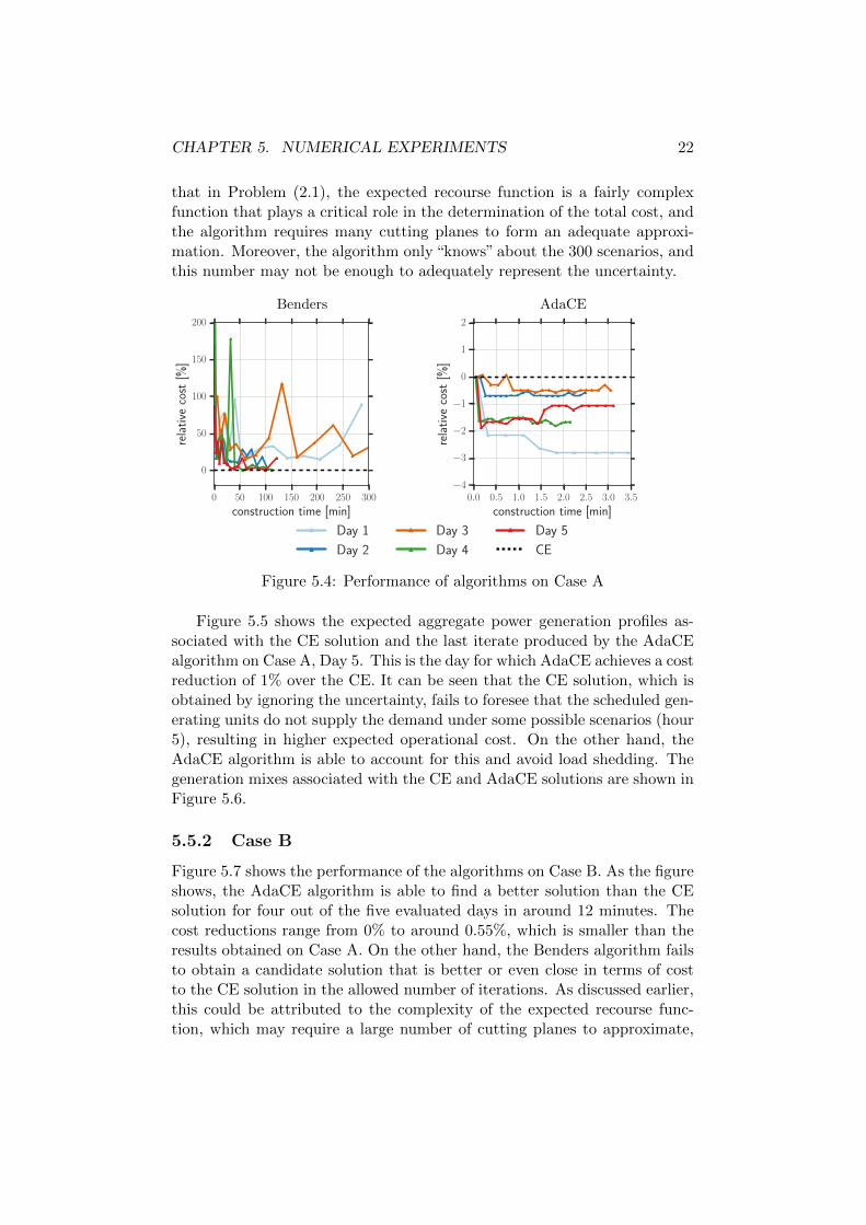
Figure 5.4 shows the performance of the algorithms on Case A. The ex-pected costs shown are relative to the cost obtained with the solution of thecertainty-equivalent (CE) problem for the corresponding day (dashed line).From the figure, several observations can be made: First, the AdaCE algo-rithm is able to exploit user-provided knowledge of the problem in the formof an initial approximation of the expected resource function, and achievecost reductions ranging from 0.5% (Day 3) to 2.8% (Day 1) relatively fast.This also shows that the CE solution is a relatively good solution for theoriginal problem under the given conditions. On the other hand, the Ben-ders algorithm struggles to find a candidate solution that is better than theCE solution on each day, with its best performance being a cost reductionof −0.5% achieved in Day 5. This outcome may be attributed to the fact


that in Problem (2.1), the expected recourse function is a fairly complexfunction that plays a critical role in the determination of the total cost, andthe algorithm requires many cutting planes to form an adequate approxi-mation. Moreover, the algorithm only “knows” about the 300 scenarios, andthis number may not be enough to adequately represent the uncertainty.

Benders

0 50 100 150 200 250 300

construction time [min]

0

50

100

150

200

rela

tive

cost

[%]

AdaCE

0.0 0.5 1.0 1.5 2.0 2.5 3.0 3.5


−4

−3

−2

−1

0

1

2

rela

tive

cost

[%]

Day 1

Day 2

Day 3

Day 4

Day 5

CE

Figure 5.4: Performance of algorithms on Case A

Figure 5.5 shows the expected aggregate power generation profiles as-sociated with the CE solution and the last iterate produced by the AdaCEalgorithm on Case A, Day 5. This is the day for which AdaCE achieves a costreduction of 1% over the CE. It can be seen that the CE solution, which isobtained by ignoring the uncertainty, fails to foresee that the scheduled gen-erating units do not supply the demand under some possible scenarios (hour5), resulting in higher expected operational cost. On the other hand, theAdaCE algorithm is able to account for this and avoid load shedding. Thegeneration mixes associated with the CE and AdaCE solutions are shown inFigure 5.6.

5.5.2 Case B

Figure 5.7 shows the performance of the algorithms on Case B. As the figureshows, the AdaCE algorithm is able to find a better solution than the CEsolution for four out of the five evaluated days in around 12 minutes. Thecost reductions range from 0% to around 0.55%, which is smaller than theresults obtained on Case A. On the other hand, the Benders algorithm failsto obtain a candidate solution that is better or even close in terms of costto the CE solution in the allowed number of iterations. As discussed earlier,this could be attributed to the complexity of the expected recourse func-tion, which may require a large number of cutting planes to approximate,


CE

5 10 15 20

time [hour]

0

20

40

60

80

100

exp

ecte

dp

ower

[%of

max

load

]AdaCE

5 10 15 20

time [hour]

0

20

40

60

80

100

exp

ecte

dp

ower

[%of

max

load

]

Generation

Demand not served

Renewable used

Renewable curtailed

Figure 5.5: Expected generation profile for Case A, Day 5

and to the insufficiency of the 300 scenarios for adequately capturing theuncertainty.

Figure 5.8 shows the expected aggregate generation profiles associatedwith the CE solution and the last iterate produced by the AdaCE algorithmon Case B, Day 1. As the figure shows, neither of these candidate solu-tions results in load shedding. Furthermore, as in Case A, the scheduledgeneration is quite flexible and is able to accommodate a high utilizationof renewable energy. The key differences between these two candidate solu-tions becomes clear when the production by technology is considered. Thisis shown in Figure 5.9. As this and Figure 5.2 show, around hour 10, whenwind production is low, and around hour 20, when wind uncertainty is highand there are sudden drops, the AdaCE solution has more flexible generat-ing units scheduled and hence is able to accommodate these changes moreefficiently.

5.5.3 Case C

As stated before, the Benders algorithm was not tested on Case C due toits poor performance on the other two test cases, which are much smaller.Instead, the impact of using the noise reduction strategy in the AdaCE al-gorithm was analyzed on this case. Figure 5.10 shows the performance ofthe AdaCE algorithm with and without noise reduction (NR) on this caseunder five different load profiles and wind distributions. It can be seen thatthe general trend is that the noise reduction strategy eventually makes theAdaCE algorithm find better commitment schedules than without it. An-other important observation is that, unlike on Cases A and B, not all can-didate solutions obtained with the AdaCE algorithm have a equal or lower


CE

5 10 15 20

time [hour]

0

1

2

3

4

5

onlin

eun

its

AdaCE

5 10 15 20

time [hour]

0

1

2

3

4

5

onlin

eun

its

5 10 15 20

time [hour]

0

20

40

60

80

100

exp

ecte

dp

ower

[%of

max

load

]

5 10 15 20

time [hour]

0

20

40

60

80

100

exp

ecte

dp

ower

[%of

max

load

]

Nuclear IGCC Coal CCGT OCGT

Figure 5.6: Generation mix for Case A, Day 5

cost compared with the CE solution, especially without noise reduction.


Benders

0 50 100 150 200 250 300


0

100

200

300

400

500

rela

tive

cost

[%]

AdaCE

0 2 4 6 8 10 12 14 16 18


−0.6

−0.5

−0.4

−0.3

−0.2

−0.1

0.0

rela

tive

cost

[%]

Day 1

Day 2

Day 3

Day 4

Day 5

CE

Figure 5.7: Performance of algorithms on Case B

CE

5 10 15 20

time [hour]

0

20

40

60

80

100

exp

ecte

dp

ower

[%of

max

load

]

AdaCE

5 10 15 20

time [hour]

0

20

40

60

80

100

exp

ecte

dp

ower

[%of

max

load

]

Generation

Demand not served

Renewable used

Renewable curtailed

Figure 5.8: Expected generation profile for Case B, Day 1


CE

5 10 15 20

time [hour]

0

10

20

30

40

50

60

onlin

eun

its

AdaCE

5 10 15 20

time [hour]

0

10

20

30

40

50

60

onlin

eun

its

5 10 15 20

time [hour]

0

20

40

60

80

100

exp

ecte

dp

ower

[%of

max

load

]

5 10 15 20

time [hour]

0

20

40

60

80

100ex

pec

ted

pow

er[%

ofm

axlo

ad]

Nuclear IGCC Coal CCGT OCGT

Figure 5.9: Generation mix for Case B, Day 1

Without NR

0 20 40 60 80 100 120 140 160


−0.3

−0.2

−0.1

0.0

0.1

0.2

rela

tive

cost

[%]

With NR

0 20 40 60 80 100 120 140 160


−0.3

−0.2

−0.1

0.0

0.1

0.2

rela

tive

cost

[%]

Day 1

Day 2

Day 3

Day 4

Day 5

CE

Figure 5.10: Performance of AdaCE on Case C

Chapter 6

Conclusions

In this work, the applicability and performance of the AdaCE algorithmfor solving the stochastic UC problem was explored. To do this, the prob-lem was first modeled as a stochastic two-stage mixed-integer optimizationproblem, which captured the essential properties that make the problemcomputationally challenging. Then, theoretical and practical issues associ-ated with the applicability of the AdaCE algorithm for solving this problemwere investigated. In particular, it was determined that the binary restric-tions present in the UC problem could make the algorithm cycle or getstuck in a sub-optimal point. Through some illustrative qualitative exam-ples, it was shown that the outcome depends heavily on the quality of theinitial approximation of the expected second-stage cost function providedto the algorithm. Furthermore, the computational challenges of the algo-rithm were investigated. It was concluded that the initial approximationsof the expected second-stage cost should be limited to be piece-wise linear,deviating from the requirements that make the algorithm work for problemswith continuous variables. To try to alleviate the computational burden ofsolving MILP problems during potentially many iterations of the algorithm,the use of noise reduction techniques was proposed. The performance ofthe algorithm was investigated along with that of a widely-used algorithmconsisting of SAA combined with Benders decomposition on test cases con-structed from three different power networks and five different load profilesand wind distributions. The results obtained showed that despite a lack oftheoretical guarantees, the AdaCE algorithm could find commitment sched-ules that are better than ones obtained with deterministic models and withthe Benders-based algorithm.

Future research steps include a sensitivity analysis of the performanceof the algorithm with respect to the number of segments of the piece-wiselinear approximations of the generator cost functions. Also, an extensionof the SHA framework that allows a richer type of updates beyond slopecorrections needs to be investigated in order to determine whether theoreti-

27

CHAPTER 6. CONCLUSIONS 28

cal guarantees can be obtained in problems with binary restrictions. Lastly,an interesting research direction consists of investigating the performanceof the AdaCE algorithm on stochastic UC problems that include market-based elements, such as power production levels in the first-stage problemand different pricing schemes.

Bibliography

[1] P. Ruiz, C. Philbrick, E. Zak, K. Cheung, and P. Sauer. Uncertaintymanagement in the unit commitment problem. IEEE Transactions onPower Systems, 24(2):642–651, May 2009.

[2] M. Tahanan, W. Van Ackooij, A. Frangioni, and F. Lacalandra. Large-scale unit commitment under uncertainty. 4OR, 13(2):115–171, 2015.

[3] Y. Chen, A. Casto, X. Wang, J. Wan, and F. Wang. Day-ahead mar-ket clearing software performance improvement. https://www.ferc.

gov/june-tech-conf/2015/abstracts/m1-2.html, 2015. [Online; ac-cessed 11-April-2017 ].

[4] International Energy Agency. System integration of renewables - Im-plications for electricity security. Technical Report to the G7, February2016. [Online; accessed 11-April-2017 ].

[5] R. Bessa, C. Moreira, B. Silva, and M. Matos. Handling renewableenergy variability and uncertainty in power systems operation. Wi-ley Interdisciplinary Reviews: Energy and Environment, 3(2):156–178,2014.

[6] P. Singhal and R. Sharma. Dynamic programming approach for largescale unit commitment problem. In International Conference on Com-munication Systems and Network Technologies, pages 714–717, June2011.

[7] A. Ott. Evolution of computing requirements in the pjm market: Pastand future. In IEEE PES General Meeting, pages 1–4, July 2010.

[8] A. Tuohy, P. Meibom, E. Denny, and M. O’Malley. Unit commitmentfor systems with significant wind penetration. IEEE Transactions onPower Systems, 24(2):592–601, May 2009.

[9] R. Ma, Y. Huang, and M. Li. Unit commitment optimal research basedon the improved genetic algorithm. In Fourth International Confer-ence on Intelligent Computation Technology and Automation, volume 1,pages 291–294, March 2011.

29

BIBLIOGRAPHY 30

[10] D. Bertsimas, E. Litvinov, X. Sun, J. Zhao, and T. Zheng. Adaptiverobust optimization for the security constrained unit commitment prob-lem. IEEE Transactions on Power Systems, 28(1):52–63, Feb 2013.

[11] W. Van Ackooij. Decomposition approaches for block-structuredchance-constrained programs with application to hydro-thermalunit commitment. Mathematical Methods of Operations Research,80(3):227–253, 2014.

[12] J. Wang, J. Wang, C. Liu, and J. Ruiz. Stochastic unit commitmentwith sub-hourly dispatch constraints. Applied Energy, 105:418 – 422,2013.

[13] L. Wu, M. Shahidehpour, and T. Li. Stochastic security-constrainedunit commitment. IEEE Transactions on Power Systems, 22(2):800–811, May 2007.

[14] A. Papavasiliou, S. Oren, and B. Rountree. Applying high performancecomputing to transmission-constrained stochastic unit commitment forrenewable energy integration. IEEE Transactions on Power Systems,30(3):1109–1120, May 2015.

[15] R. Cheung and W. Powell. SHAPE - A stochastic hybrid approximationprocedure for two-stage stochastic programs. Operations. Research.,48(1):73–79, 2000.

[16] T. Tinoco De Rubira and G. Hug. Adaptive certainty-equivalent ap-proach for optimal generator dispatch under uncertainty. In EuropeanControl Conference (ECC), pages 1215–1222, June 2016.

[17] T. Tinoco De Rubira and G. Hug. Primal-dual stochastic hybrid ap-proximation algorithm. Computational Optimization and Applications(under review), 2016.

[18] T. Tinoco De Rubira, L. Roald, and G. Hug. Multi-stage stochastic op-timization via parameterized stochastic hybrid approximation. (underreview).

[19] H. Dai, N. Zhang, and W. Su. A literature review of stochastic program-ming and unit commitment. Journal of Power and Energy Engineering,3:206–214, 2015.

[20] European Commission. Launching the public consultation processon a new energy market design. Technical Report SWD(2015) 142Final, January 2015. https://ec.europa.eu/energy/sites/ener/

files/publication/web_1_EN_ACT_part1_v11_en.pdf, [Online; ac-cessed 11-April-2017].

BIBLIOGRAPHY 31

[21] J. Zhu. Optimization of Power System Operation. John Wiley & Sons,Inc., 2009.

[22] J. R. Birge and F. Louveaux. Introduction to Stochastic Program-ming. Springer Series in Operations Research and Financial Engineer-ing, 2011.

[23] T. Homem de Mello and G. Bayraksan. Monte carlo sampling-basedmethods for stochastic optimization. Surveys in Operations Researchand Management Science, 19(1):56 – 85, 2014.

[24] H. Kushner and G. Yin. Stochastic Approximation and Recursive Algo-rithms and Applications. Stochastic Modelling and Applied Probability.Springer-Verlag, 2003.

[25] F. Louveaux. Piecewise convex programs. Mathematical Programming,15(1):53–62, 1978.

[26] R. Byrd, G. Chin, J. Nocedal, and Y. Wu. Sample size selection in op-timization methods for machine learning. Mathematical Programming,134(1):127–155, 2012.

[27] S. Diamond and S. Boyd. CVXPY: A Python-embedded modeling lan-guage for convex optimization. Journal of Machine Learning Research,17(83):1–5, 2016.

[28] Gurobi Optimization, Inc. Gurobi optimizer reference manual, 2016.

[29] A. Domahidi, E. Chu, and S. Boyd. ECOS: An SOCP solver for embed-ded systems. In European Control Conference (ECC), pages 3071–3076,2013.

[30] C. Josz, S. Fliscounakis, J. Maeght, and P. Panciatici. AC power flowdata in MATPOWER and QCQP format: iTesla, RTE snapshots, andPEGASE, 2016. arXiv:1603.01533.

[31] C. Grigg, P. Wong, P. Albrecht, R. Allan, M. Bhavaraju, R. Billinton,Q. Chen, C. Fong, S. Haddad, S. Kuruganty, W. Li, R. Mukerji, D. Pat-ton, N. Rau, D. Reppen, A. Schneider, M. Shahidehpour, and C. Singh.The ieee reliability test system-1996. A report prepared by the reliabilitytest system task force of the application of probability methods subcom-mittee. IEEE Transactions on Power Systems, 14(3):1010–1020, Aug1999.

[32] Black and Veatch Holding Company. Cost and performance data forpower generation technologies. Prepared for the National RenewableEnergy Laboratory. https://www.bv.com/docs/reports-studies/

nrel-cost-report.pdf, [Online; accessed 11-April-2017].

Analysis of Adaptive Certainty-Equivalent … of Adaptive Certainty-Equivalent Techniques for ... in...

Documents

Transcript of Analysis of Adaptive Certainty-Equivalent … of Adaptive Certainty-Equivalent Techniques for ... in...