By Riyaj Shamsudeen - Oracle database internals by Riyaj · PDF file©OraInternals Riyaj...

©OraInternals Riyaj Shamsudeen

Performance tuning for developers

By Riyaj Shamsudeen

©OraInternals Riyaj Shamsudeen 2

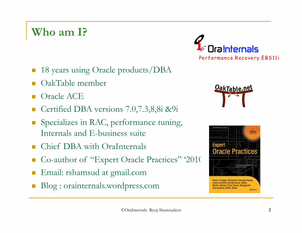
Who am I?

  18 years using Oracle products/DBA   OakTable member   Oracle ACE   Certified DBA versions 7.0,7.3,8,8i &9i   Specializes in RAC, performance tuning,

Internals and E-business suite   Chief DBA with OraInternals   Co-author of “Expert Oracle Practices” ‘2010   Email: rshamsud at gmail.com   Blog : orainternals.wordpress.com


Disclaimer

These slides and materials represent the work and opinions of the author and do not constitute official positions of my current or past employer or any other organization. This material has been peer reviewed, but author assume no responsibility whatsoever for the test cases.

If you corrupt your databases by running my scripts, you are solely responsible for that.

This material should not should not be reproduced or used without the authors' written permission.


Agenda

  Tracing SQL execution

  Analyzing Trace files

  Understanding Explain plans

  Joins

  Writing optimal SQL

  Good hints and no-so good hints

  Effective indexing

  Partitioning for performance


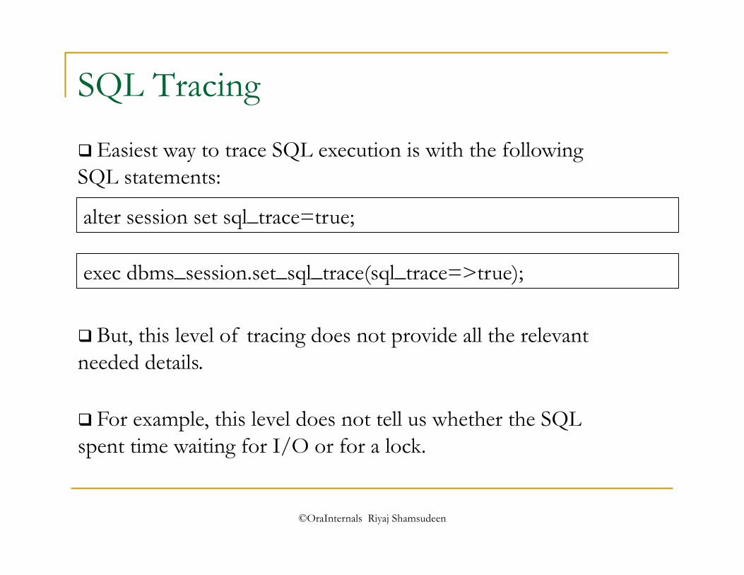
SQL Tracing

  Easiest way to trace SQL execution is with the following SQL statements:

  But, this level of tracing does not provide all the relevant needed details.

  For example, this level does not tell us whether the SQL spent time waiting for I/O or for a lock.

alter session set sql_trace=true;

exec dbms_session.set_sql_trace(sql_trace=>true);


Waits

  SQL statement execution is in one of two states (We will ignore OS scheduling waits for now):

  On CPU executing the statement (or)   Waiting for an event such as I/O, lock etc.

  If you don’t know where the time is spent, you can reduce the time spent scientifically.

  For example, SQL statement waiting for I/O will wait for one of these events:

  db file sequential read   db file scattered read etc.


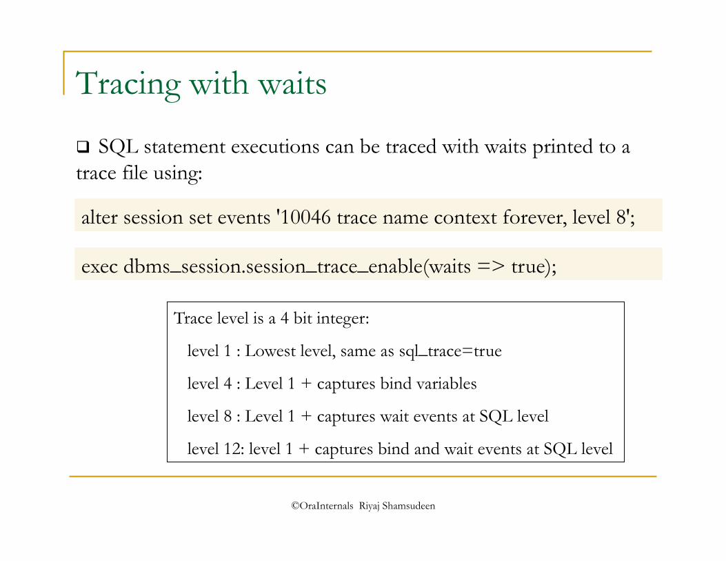
Tracing with waits

  SQL statement executions can be traced with waits printed to a trace file using:

alter session set events '10046 trace name context forever, level 8';

exec dbms_session.session_trace_enable(waits => true);

Trace level is a 4 bit integer:

level 1 : Lowest level, same as sql_trace=true

level 4 : Level 1 + captures bind variables

level 8 : Level 1 + captures wait events at SQL level

level 12: level 1 + captures bind and wait events at SQL level


Trace file explained …1 PARSING IN CURSOR #3 len=83 dep=0 uid=173 oct=3 lid=173 tim=12972441295985 hv=855947554 ad='fa2e5530' select transaction_id from mtl_transaction_accounts where transaction_id=1682944981 END OF STMT PARSE #3:c=10000,e=5080,p=0,cr=0,cu=0,mis=1,r=0,dep=0,og=1,tim=12972441295971 EXEC #3:c=0,e=198,p=0,cr=0,cu=0,mis=0,r=0,dep=0,og=1,tim=12972441296397 WAIT #3: nam='SQL*Net message to client' ela= 8 driver id=1650815232 #bytes=1 p3=0 obj#=38149 tim=12972441296513 WAIT #3: nam='db file sequential read' ela= 8337 file#=803 block#=213006 blocks=1 obj#=38172 tim=12972441305307 WAIT #3: nam='db file sequential read' ela= 12840 file#=234 block#=65037 blocks=1 obj#=38172 tim=12972441318487 WAIT #3: nam='gc cr grant 2-way' ela= 807 p1=803 p2=213474 p3=1 obj#=38172 tim=12972441320096 WAIT #3: nam='db file sequential read' ela= 4095 file#=803 block#=213474 blocks=1 obj#=38172 tim=12972441324278

  Highlighted lines indicates that SQL statement is being parsed.


Trace file explained …2 PARSING IN CURSOR #3 len=83 dep=0 uid=173 oct=3 lid=173 tim=12972441295985 hv=855947554 ad='fa2e5530' select transaction_id from mtl_transaction_accounts where transaction_id=1682944981 END OF STMT PARSE #3:c=10000,e=5080,p=0,cr=0,cu=0,mis=1,r=0,dep=0,og=1,tim=12972441295971 EXEC #3:c=0,e=198,p=0,cr=0,cu=0,mis=0,r=0,dep=0,og=1,tim=12972441296397 WAIT #3: nam='SQL*Net message to client' ela= 8 driver id=1650815232 #bytes=1 p3=0 obj#=38149 tim=12972441296513

WAIT #3: nam='db file sequential read' ela= 8337 file#=803 block#=213006 blocks=1 obj#=38172 tim=12972441305307 WAIT #3: nam='db file sequential read' ela= 12840 file#=234 block#=65037 blocks=1 obj#=38172 tim=12972441318487 WAIT #3: nam='db file sequential read' ela= 4095 file#=803 block#=213474 blocks=1 obj#=38172 tim=12972441324278

Event waited for Elapsed time (micro seconds)

  Later, we will show how tkprof utility can aggregate these events and print formatted output.


Tracing with binds

  SQL statement executions can be traced with bind variable values also:

alter session set events '10046 trace name context forever, level 12';

exec dbms_session.session_trace_enable(waits => true,binds=>true);

  Generally, you wouldn’t need to trace with binds unless you want to find the bind variables also.

  If there are many executions of SQL statements (millions) in a process then turning on trace with binds can reduce performance.


Agenda




  Joins






tkprof

  Trace files generated from SQLTrace is not exactly readable.

tkprof trace_file outfile sort=option explain=user/pwd sys=no

  tkprof utility provides formatted output from the trace files.

tkprof devl_ora_123.trc /tmp/devl_ora_tkp.out sort=exeela,fchela Example:

  tkprof comes with help options. Just type tkprof and enter to see help.


Sort option

  Sort option in tkprof is useful. For example, sort=exeela will sort the SQL statements by Elapsed time at execution step.

  Top SQL statements by elapsed time will show up at the top of the tkprof output file.

  Generally, I use sort=exeela, fchela to sort the SQL statements.

  Other common options are: execpu, fchcpu, prsela etc.


explain option

  But, SQL Trace also prints execution plan in the trace file.

  Explain=userid/password@dev can be supplied to print execution plan of that SQL statement.

  Explain option logs on to the database and executes explain plan for every SQL in the trace file.

  It is a good practice not to use explain option and use the execution plan in the trace file itself.

  If you are using SQLPlus or TOAD to execute SQL, make sure to close the connection or exit so that trace files will be complete.


More on tracing…

  Trace at program level

  Using alter session command:

alter session set events ' 10046 trace name context forever, level 12';

 Using dbms_system in another session (mostly used by DBAs):

Exec dbms_System.set_ev( sid, serial#, 10046, 12, '');

Exec dbms_System.set_Sql_Trace_in_session(sid, serial#, true);


Agenda




  Joins






Execution plan

  Understanding execution plan is an important step in resolving performance issues.

explain plan for select t1.id, t1.vc10 , t2.id From t1,t2 where t1.id=t2.id and t2.id <1000;

Select * from table(dbms_xplan.display);

  There are many ways to generate execution plans and easiest way is (Not necessarily always correct as we see later):


Simple SELECT Select * from table(dbms_xplan.display);

-------------------------------------------------------------------------------------- | Id | Operation | Name | Rows | Bytes | Cost (%CPU)| Time |

-------------------------------------------------------------------------------------- | 0 | SELECT STATEMENT | | 975 | 22425 | 512 (1)| 00:00:02 | |* 1 | HASH JOIN | | 975 | 22425 | 512 (1)| 00:00:02 |

|* 2 | INDEX RANGE SCAN | T2_N1 | 976 | 5856 | 5 (0)| 00:00:01 | | 3 | TABLE ACCESS BY INDEX ROWID| T1 | 1000 | 17000 | 506 (1)| 00:00:02 |

|* 4 | INDEX RANGE SCAN | T1_N1 | 1000 | | 5 (0)| 00:00:01 | --------------------------------------------------------------------------------------

Predicate Information (identified by operation id): ---------------------------------------------------

1 - access("T1"."ID"="T2"."ID") 2 - access("T2"."ID"<1000) 4 - access("T1"."ID"<1000)

(i) Index T2_N1 was scanned with access predicate t2.id <1000 [ Step 2] (ii) Index T1_N1 was scanned with access predicate t1.id <1000 [ Step 4] (iii) Table T1 is accessed to retrieve non-indexed column using rowids returned from step 2. [ Step 3]. (iv) Rows from step 2 and 3 are joined to create the final result set.[Step 1]

Execution sequence


Predicates

Set lines 120 pages 0


------------------------------------------------------------------------------------------------------ | Id | Operation | Name | Rows | Bytes | Cost (%CPU)| ------------------------------------------------------------------------------------------------------ | 0 | SELECT STATEMENT | | 1 | 214 | 9 (23)| | 1 | SORT ORDER BY | | 1 | 214 | 9 (23)| |* 2 | TABLE ACCESS BY INDEX ROWID | RCV_STAGING_LINES | 1 | 155 | 4 (25)| | 3 | NESTED LOOPS | | 1 | 214 | 8 (13)| |* 4 | TABLE ACCESS BY INDEX ROWID| RCV_STAGING_HEADERS | 1 | 59 | 5 (20)| |* 5 | INDEX RANGE SCAN | RCV_STAGING_HEADERS_N5 | 20 | | 4 (25)| |* 6 | INDEX RANGE SCAN | RCV_STAGING_LINES_N3 | 1 | | 3 (34)| ------------------------------------------------------------------------------------------------------

Predicate Information (identified by operation id): --------------------------------------------------- 2 - filter("RSL"."RMA_NUMBER"=:Z AND "RSL"."RMA_LINE_NUMBER"=TO_NUMBER(:Z))

4 - filter("RSH"."RMA_NUMBER"=:Z AND "RSH"."REQUEST_ID"=TO_NUMBER(:Z)) 5 - access("RSH"."STATUS"='PROCESSED')

6 - access("RSH"."SOURCE_HEADER_ID"="RSL"."SOURCE_HEADER_ID")

  Predicates are very useful to debug performance issues.

  Cardinality estimate is a good guess. 20 rows are returned in step 5 , but just one row returned from the table (step 4).


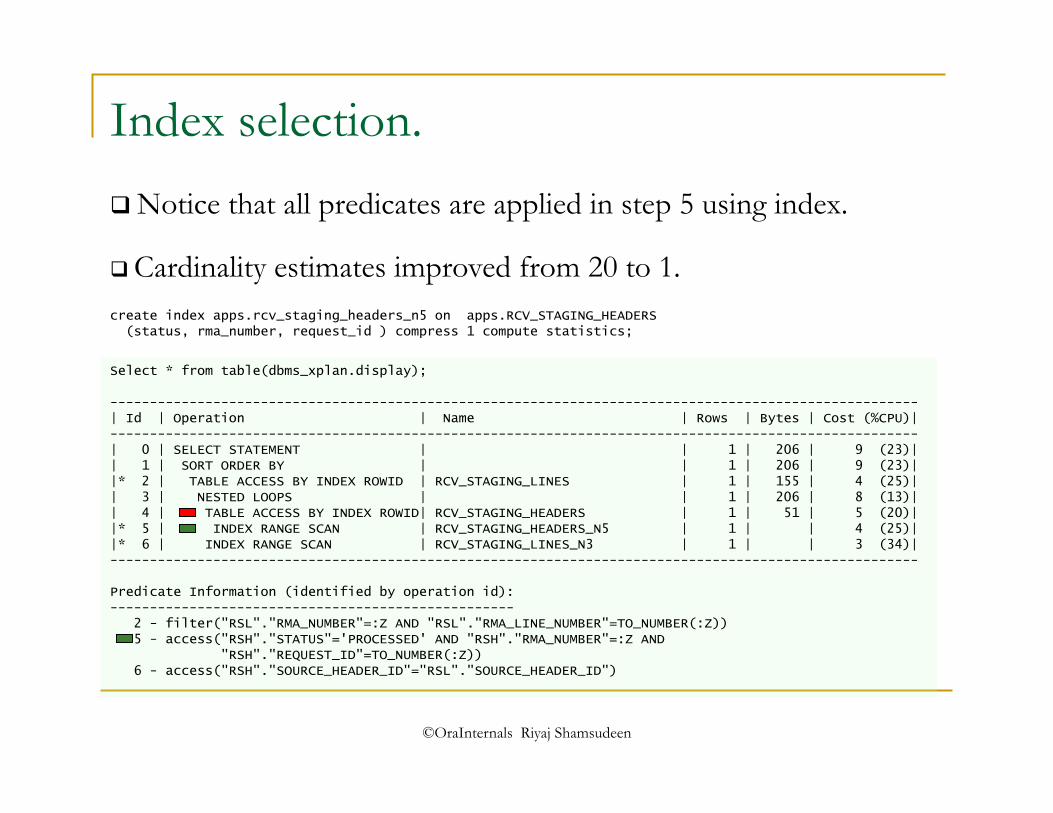
Index selection.


------------------------------------------------------------------------------------------------------ | Id | Operation | Name | Rows | Bytes | Cost (%CPU)| ------------------------------------------------------------------------------------------------------ | 0 | SELECT STATEMENT | | 1 | 206 | 9 (23)| | 1 | SORT ORDER BY | | 1 | 206 | 9 (23)| |* 2 | TABLE ACCESS BY INDEX ROWID | RCV_STAGING_LINES | 1 | 155 | 4 (25)| | 3 | NESTED LOOPS | | 1 | 206 | 8 (13)| | 4 | TABLE ACCESS BY INDEX ROWID| RCV_STAGING_HEADERS | 1 | 51 | 5 (20)| |* 5 | INDEX RANGE SCAN | RCV_STAGING_HEADERS_N5 | 1 | | 4 (25)| |* 6 | INDEX RANGE SCAN | RCV_STAGING_LINES_N3 | 1 | | 3 (34)| ------------------------------------------------------------------------------------------------------

Predicate Information (identified by operation id): --------------------------------------------------- 2 - filter("RSL"."RMA_NUMBER"=:Z AND "RSL"."RMA_LINE_NUMBER"=TO_NUMBER(:Z)) 5 - access("RSH"."STATUS"='PROCESSED' AND "RSH"."RMA_NUMBER"=:Z AND "RSH"."REQUEST_ID"=TO_NUMBER(:Z)) 6 - access("RSH"."SOURCE_HEADER_ID"="RSL"."SOURCE_HEADER_ID")

create index apps.rcv_staging_headers_n5 on apps.RCV_STAGING_HEADERS (status, rma_number, request_id ) compress 1 compute statistics;

  Notice that all predicates are applied in step 5 using index.

  Cardinality estimates improved from 20 to 1.


Package: dbms_xplan

  Dbms_xplan is a package available from 9i. It has many rich features.

  dbms_xplan package has following features:   Print execution plan for recently explained SQL statement:

dbms_xplan.display;   Print execution plan for a SQL statement executed by passing sql_id or hash_value:

dbms_xplan.display_cursor ('&sqlid', '', '');   Print execution plan for a SQL statement captured by AWR report:

dbms_xplan.display_awr ('&sqlid', '', '');


Autotrace deprecated

  Many of us are used to autotrace in SQL*Plus. Use dbms_xplan instead ( from 10g onwards):

select t1.id, t1.vc10 , t2.id From t1,t2 where t1.id=t2.id and t2.id <1000;

Select * from table (dbms_xplan.display_cursor);

SQL_ID cd6h52abfgfg3, child number 0 ------------------------------------- select t1.id, t1.vc10 , t2.id From t1,t2 where t1.id=t2.id and t2.id <1000

Plan hash value: 3286489634 -------------------------------------------------------------------------- | Id | Operation | Name | Rows | Bytes | Cost (%CPU)| Time | --------------------------------------------------------------------------- | 0 | SELECT STATEMENT | | | | 512 (100)| | |* 1 | HASH JOIN | | 975 | 22425 | 512 (1)| 00:00:02 | ...


But..   dbms_xplan accesses v$sql, v$sql_plan_statistics_all and v$sql_plan internally. So, you need to have select access on these fixed views to execute dbms_xplan.

  Executing dbms_xplan.display_cursor without specifying any sql_id retrieves the execution plan for the query executed last.

  From 10g onwards, serveroutput is on by default. You need to disable serveroutput to see the execution plan correctly:

Select * from table (dbms_xplan.display_cursor);

SQL_ID 9babjv8yq8ru3, child number 1 BEGIN DBMS_OUTPUT.GET_LINES(:LINES, :NUMLINES); END;


Display_cursor   Suppose, you want to find the execution plan of a SQL statement executed recently, then display_cursor is handy.

  Find sql_id or hash_value of the SQL statement from v$sql and pass that to display_cursor:

select * from table(dbms_xplan.display_cursor ( '&sql_id','',''));

SQL_ID fqmkvmdyb043r, child number 0

------------------------------------- select t1.id, t1.vc10 , t2.id From t1,t2 where t1.id=t2.id and t2.id <1000

Plan hash value: 3286489634 --------------------------------------------------------------------------------------

| Id | Operation | Name | Rows | Bytes | Cost (%CPU)| Time | -------------------------------------------------------------------------------------- | 0 | SELECT STATEMENT | | | | 512 (100)| |

|* 1 | HASH JOIN | | 975 | 22425 | 512 (1)| 00:00:02 | |* 2 | INDEX RANGE SCAN | T2_N1 | 976 | 5856 | 5 (0)| 00:00:01 |

| 3 | TABLE ACCESS BY INDEX ROWID| T1 | 1000 | 17000 | 506 (1)| 00:00:02 | ...


Time spent?

Rows Row Source Operation ------- --------------------------------------------------- 49996 WINDOW SORT 644538 NESTED LOOPS 704891 NESTED LOOPS 704891 NESTED LOOPS 704891 NESTED LOOPS OUTER 704891 NESTED LOOPS 704891 NESTED LOOPS 1 TABLE ACCESS BY INDEX ROWID HR_ALL_ORGANIZATION_UNITS 1 INDEX UNIQUE SCAN HR_ORGANIZATION_UNITS_PK 704891 TABLE ACCESS BY INDEX ROWID WSH_DELIVERY_DETAILS 704891 INDEX RANGE SCAN WSH_DELIVERY_DETAILS_N8 704891 TABLE ACCESS BY INDEX ROWID MTL_SYSTEM_ITEMS_B 704891 INDEX RANGE SCAN MTL_SYSTEM_ITEMS_B_U1 644783 VIEW PUSHED PREDICATE 644783 NESTED LOOPS 704891 TABLE ACCESS BY INDEX ROWID FND_FLEX_VALUE_SETS 704891 INDEX UNIQUE SCAN FND_FLEX_VALUE_SETS_U2 644783 TABLE ACCESS BY INDEX ROWID FND_FLEX_VALUES 644783 INDEX RANGE SCAN FND_FLEX_VALUES_N1 704891 TABLE ACCESS BY INDEX ROWID OE_ORDER_LINES_ALL 704891 INDEX UNIQUE SCAN OE_ORDER_LINES_U1 704891 TABLE ACCESS BY INDEX ROWID WSH_DELIVERY_ASSIGNMENTS 704891 INDEX RANGE SCAN WSH_DELIVERY_ASSIGNMENTS_N3 644538 TABLE ACCESS BY INDEX ROWID WSH_NEW_DELIVERIES 704891 INDEX UNIQUE SCAN WSH_NEW_DELIVERIES_U1

Total of 330 seconds spent on this SQL. Can you identify the step that incurred most time?


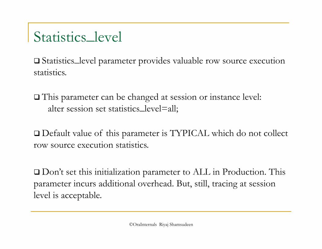
Statistics_level   Statistics_level parameter provides valuable row source execution statistics.

  This parameter can be changed at session or instance level: alter session set statistics_level=all;

  Default value of this parameter is TYPICAL which do not collect row source execution statistics.

  Don’t set this initialization parameter to ALL in Production. This parameter incurs additional overhead. But, still, tracing at session level is acceptable.


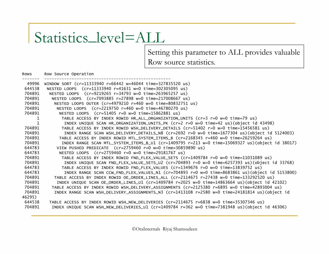
Statistics_level=ALL

Rows Row Source Operation ------- --------------------------------------------------- 49996 WINDOW SORT (cr=11333940 r=66442 w=46044 time=327835520 us) 644538 NESTED LOOPS (cr=11333940 r=41631 w=0 time=302305095 us) 704891 NESTED LOOPS (cr=9219265 r=34793 w=0 time=263965257 us) 704891 NESTED LOOPS (cr=7093885 r=27898 w=0 time=217008667 us) 704891 NESTED LOOPS OUTER (cr=4979210 r=460 w=0 time=80832751 us) 704891 NESTED LOOPS (cr=2219750 r=460 w=0 time=46780270 us) 704891 NESTED LOOPS (cr=51405 r=0 w=0 time=15862881 us) 1 TABLE ACCESS BY INDEX ROWID HR_ALL_ORGANIZATION_UNITS (cr=3 r=0 w=0 time=79 us) 1 INDEX UNIQUE SCAN HR_ORGANIZATION_UNITS_PK (cr=2 r=0 w=0 time=42 us)(object id 43498) 704891 TABLE ACCESS BY INDEX ROWID WSH_DELIVERY_DETAILS (cr=51402 r=0 w=0 time=15456581 us) 704891 INDEX RANGE SCAN WSH_DELIVERY_DETAILS_N8 (cr=2692 r=0 w=0 time=1677304 us)(object id 5124003) 704891 TABLE ACCESS BY INDEX ROWID MTL_SYSTEM_ITEMS_B (cr=2168345 r=460 w=0 time=26259264 us) 704891 INDEX RANGE SCAN MTL_SYSTEM_ITEMS_B_U1 (cr=1409795 r=213 w=0 time=15069327 us)(object id 38017) 644783 VIEW PUSHED PREDICATE (cr=2759460 r=0 w=0 time=30859890 us) 644783 NESTED LOOPS (cr=2759460 r=0 w=0 time=29181767 us) 704891 TABLE ACCESS BY INDEX ROWID FND_FLEX_VALUE_SETS (cr=1409784 r=0 w=0 time=11031089 us) 704891 INDEX UNIQUE SCAN FND_FLEX_VALUE_SETS_U2 (cr=704893 r=0 w=0 time=6257393 us)(object id 33768) 644783 TABLE ACCESS BY INDEX ROWID FND_FLEX_VALUES (cr=1349676 r=0 w=0 time=13839752 us) 644783 INDEX RANGE SCAN CCW_FND_FLEX_VALUES_N1 (cr=704893 r=0 w=0 time=8683861 us)(object id 5153800) 704891 TABLE ACCESS BY INDEX ROWID OE_ORDER_LINES_ALL (cr=2114675 r=27438 w=0 time=133292520 us) 704891 INDEX UNIQUE SCAN OE_ORDER_LINES_U1 (cr=1409784 r=2025 w=0 time=14863664 us)(object id 42102) 704891 TABLE ACCESS BY INDEX ROWID WSH_DELIVERY_ASSIGNMENTS (cr=2125380 r=6895 w=0 time=42893004 us) 704891 INDEX RANGE SCAN WSH_DELIVERY_ASSIGNMENTS_N3 (cr=1413108 r=2580 w=0 time=24181814 us)(object id 46295) 644538 TABLE ACCESS BY INDEX ROWID WSH_NEW_DELIVERIES (cr=2114675 r=6838 w=0 time=35307346 us) 704891 INDEX UNIQUE SCAN WSH_NEW_DELIVERIES_U1 (cr=1409784 r=362 w=0 time=7381948 us)(object id 46306)

Setting this parameter to ALL provides valuable Row source statistics.


Statistics_level=ALL

Rows Row Source Operation ------- --------------------------------------------------- 49996 WINDOW SORT (cr=11333940 r=66442 w=46044 time=327835520 us) 644538 NESTED LOOPS (cr=11333940 r=41631 w=0 time=302305095 us) 704891 NESTED LOOPS (cr=9219265 r=34793 w=0 time=263965257 us) 704891 NESTED LOOPS (cr=7093885 r=27898 w=0 time=217008667 us) 704891 NESTED LOOPS OUTER (cr=4979210 r=460 w=0 time=80832751 us) 704891 NESTED LOOPS (cr=2219750 r=460 w=0 time=46780270 us) 704891 NESTED LOOPS (cr=51405 r=0 w=0 time=15862881 us) 1 TABLE ACCESS BY INDEX ROWID HR_ALL_ORGANIZATION_UNITS (cr=3 r=0 w=0 time=79 us) 1 INDEX UNIQUE SCAN HR_ORGANIZATION_UNITS_PK (cr=2 r=0 w=0 time=42 us)(object id 43498) 704891 TABLE ACCESS BY INDEX ROWID WSH_DELIVERY_DETAILS (cr=51402 r=0 w=0 time=15456581 us) 704891 INDEX RANGE SCAN WSH_DELIVERY_DETAILS_N8 (cr=2692 r=0 w=0 time=1677304 us)(object id 5124003) 704891 TABLE ACCESS BY INDEX ROWID MTL_SYSTEM_ITEMS_B (cr=2168345 r=460 w=0 time=26259264 us) 704891 INDEX RANGE SCAN MTL_SYSTEM_ITEMS_B_U1 (cr=1409795 r=213 w=0 time=15069327 us)(object id 38017) 644783 VIEW PUSHED PREDICATE (cr=2759460 r=0 w=0 time=30859890 us) 644783 NESTED LOOPS (cr=2759460 r=0 w=0 time=29181767 us) 704891 TABLE ACCESS BY INDEX ROWID FND_FLEX_VALUE_SETS (cr=1409784 r=0 w=0 time=11031089 us) 704891 INDEX UNIQUE SCAN FND_FLEX_VALUE_SETS_U2 (cr=704893 r=0 w=0 time=6257393 us)(object id 33768) 644783 TABLE ACCESS BY INDEX ROWID FND_FLEX_VALUES (cr=1349676 r=0 w=0 time=13839752 us) 644783 INDEX RANGE SCAN CCW_FND_FLEX_VALUES_N1 (cr=704893 r=0 w=0 time=8683861 us)(object id 5153800) 704891 TABLE ACCESS BY INDEX ROWID OE_ORDER_LINES_ALL (cr=2114675 r=27438 w=0 time=133292520 us) 704891 INDEX UNIQUE SCAN OE_ORDER_LINES_U1 (cr=1409784 r=2025 w=0 time=14863664 us)(object id 42102) 704891 TABLE ACCESS BY INDEX ROWID WSH_DELIVERY_ASSIGNMENTS (cr=2125380 r=6895 w=0 time=42893004 us) 704891 INDEX RANGE SCAN WSH_DELIVERY_ASSIGNMENTS_N3 (cr=1413108 r=2580 w=0 time=24181814 us)(object id 46295) 644538 TABLE ACCESS BY INDEX ROWID WSH_NEW_DELIVERIES (cr=2114675 r=6838 w=0 time=35307346 us) 704891 INDEX UNIQUE SCAN WSH_NEW_DELIVERIES_U1 (cr=1409784 r=362 w=0 time=7381948 us)(object id 46306)

Timeline


Statistics_level

  So, statistics_level parameter can be used to understand the step consuming much time.

  To improve performance we try to reduce the step consuming time.

  But, of course, functional knowledge of the SQL statement will come handy.


All trace commands   If you are tracing from your session, you might want to set these parameters too:

  Sets maximum file size to unlimited.

Alter session set max_dump_file_size=unlimited;

  This sets trace files to have file names easily distinguishable!

alter session set tracefile_identifier='riyaj';

  Print row source timing information.

alter session set Statistics_level=all;

exec dbms_session.session_trace_enable(waits => true);


Agenda




  Access, Joins, filters and unnest






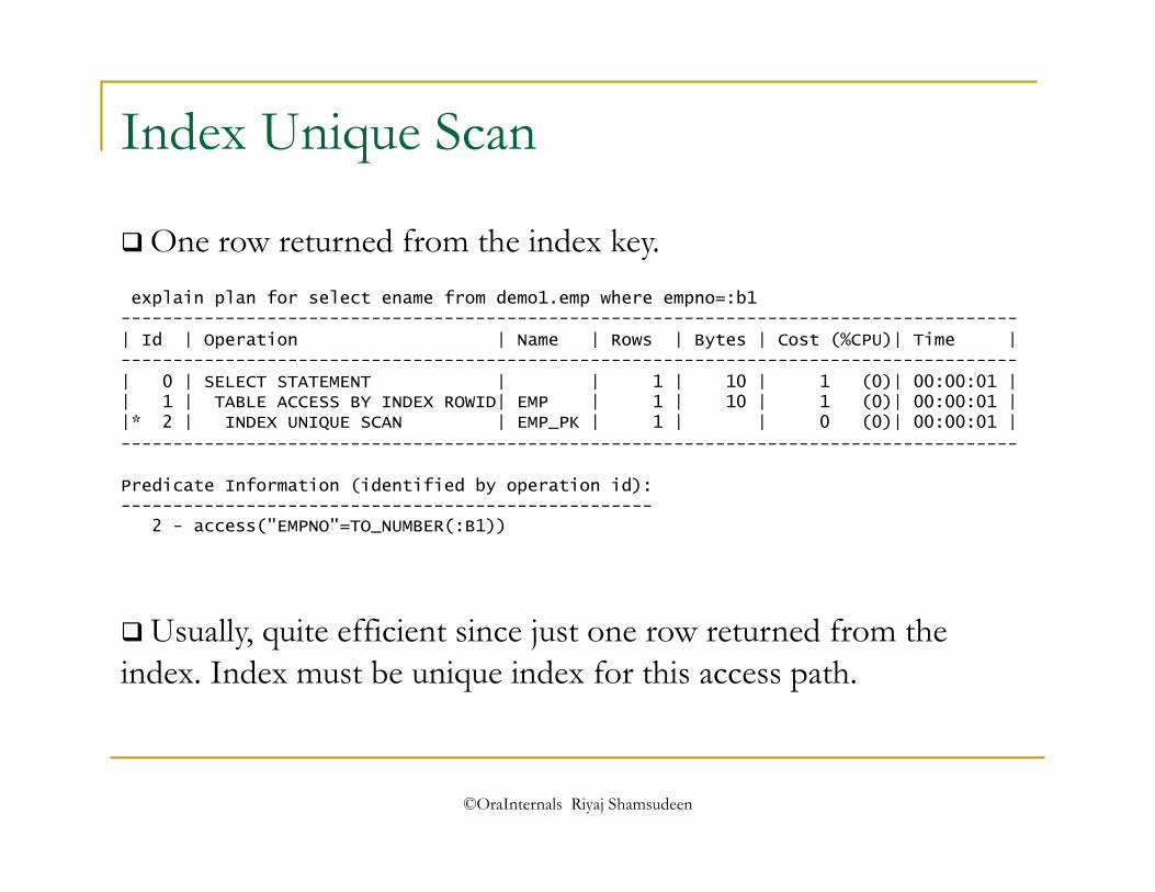
Index Unique Scan

explain plan for select ename from demo1.emp where empno=:b1 --------------------------------------------------------------------------------------

| Id | Operation | Name | Rows | Bytes | Cost (%CPU)| Time | --------------------------------------------------------------------------------------

| 0 | SELECT STATEMENT | | 1 | 10 | 1 (0)| 00:00:01 | | 1 | TABLE ACCESS BY INDEX ROWID| EMP | 1 | 10 | 1 (0)| 00:00:01 | |* 2 | INDEX UNIQUE SCAN | EMP_PK | 1 | | 0 (0)| 00:00:01 |

--------------------------------------------------------------------------------------

Predicate Information (identified by operation id): --------------------------------------------------- 2 - access("EMPNO"=TO_NUMBER(:B1))

  One row returned from the index key.

  Usually, quite efficient since just one row returned from the index. Index must be unique index for this access path.


Index unique scan

Index returns one Rowid.

Table Root block

Branch block

Leaf blocks

empno:b1

Data file

120

121

122

123

124

125

126


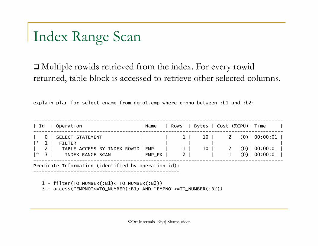
Index Range Scan

explain plan for select ename from demo1.emp where empno between :b1 and :b2;

---------------------------------------------------------------------------------------

| Id | Operation | Name | Rows | Bytes | Cost (%CPU)| Time | --------------------------------------------------------------------------------------- | 0 | SELECT STATEMENT | | 1 | 10 | 2 (0)| 00:00:01 |

|* 1 | FILTER | | | | | | | 2 | TABLE ACCESS BY INDEX ROWID| EMP | 1 | 10 | 2 (0)| 00:00:01 |

|* 3 | INDEX RANGE SCAN | EMP_PK | 2 | | 1 (0)| 00:00:01 | --------------------------------------------------------------------------------------- Predicate Information (identified by operation id):

---------------------------------------------------

1 - filter(TO_NUMBER(:B1)<=TO_NUMBER(:B2)) 3 - access("EMPNO">=TO_NUMBER(:B1) AND "EMPNO"<=TO_NUMBER(:B2))

  Multiple rowids retrieved from the index. For every rowid returned, table block is accessed to retrieve other selected columns.


Index range scan

Index may return one or more rowids.

Table Root block

Branch block

Leaf blocks

Empno between :b1 and :b2

Data file

120

121

122

123

124

125

126


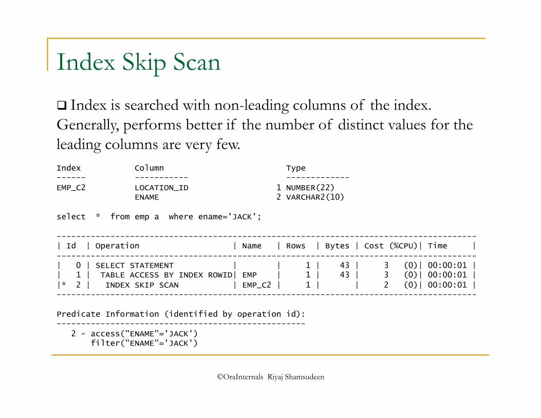
Index Skip Scan

Index Column Type ------ ----------- -------------

EMP_C2 LOCATION_ID 1 NUMBER(22) ENAME 2 VARCHAR2(10)

select * from emp a where ename='JACK';

-------------------------------------------------------------------------------------- | Id | Operation | Name | Rows | Bytes | Cost (%CPU)| Time |

-------------------------------------------------------------------------------------- | 0 | SELECT STATEMENT | | 1 | 43 | 3 (0)| 00:00:01 | | 1 | TABLE ACCESS BY INDEX ROWID| EMP | 1 | 43 | 3 (0)| 00:00:01 |

|* 2 | INDEX SKIP SCAN | EMP_C2 | 1 | | 2 (0)| 00:00:01 | --------------------------------------------------------------------------------------


2 - access("ENAME"='JACK') filter("ENAME"='JACK')

  Index is searched with non-leading columns of the index. Generally, performs better if the number of distinct values for the leading columns are very few.


Index skip scan

Leading column Is location_id

Table Root block

Branch block

Leaf blocks

Empname=‘JACK’

Data file

120

121

122

123

124

125

126


Joins

  Type of join operators   Equi-join   Outer join   Merge Join   Anti-join

  Type of join techniques in Oracle   Nested Loops join   Hash Join   Merge Join


Nested loops join

644783 NESTED LOOPS 704891 TABLE ACCESS BY INDEX ROWID EMP 704891 INDEX UNIQUE SCAN EMP_C1 644783 TABLE ACCESS BY INDEX ROWID EMP_HISTORY 644783 INDEX RANGE SCAN EMP_HIST_N1

  For every row from outer row source, inner row source is probed for a matching row satisfying join key condition.

  Generally, performs better if number of rows from the inner row source is much lower.

  Typically, OLTP uses this type of join.


Nested loops join

EMP_C1 Index searched for the predicate Emp_name like ‘S%’

EMP

Rowids fetched from the index and table accessed.

Loop

EMP_HIST_N1

EMP_HISTORY

Rowids fetched from the index and table accessed using rowid.

Index searched for the join key Employee_id = employee_id

Row piece fetched from the table


1

2

3

4

5

6

7

644783 NESTED LOOPS 704891 TABLE ACCESS BY INDEX ROWID EMP 704891 INDEX UNIQUE SCAN EMP_C1

644783 TABLE ACCESS BY INDEX ROWID EMP_HISTORY 644783 INDEX RANGE SCAN EMP_HIST_N1


Hash join

explain plan for select t1.color, t2.color, t1.shape from t1, t2 where t1.color_id = t2.color_id and t1.color=:b1 and t2.color=:b1 / Explained.

SQL> select * from table (dbms_xplan.display);

Plan hash value: 2339531555

------------------------------------------------------------------d----------------------- | Id | Operation | Name | Rows | Bytes | Cost (%CPU)| Time | ----------------------------------------------------------------------------------------- | 0 | SELECT STATEMENT | | 333 | 9990 | 8 (13)| 00:00:01 | |* 1 | HASH JOIN | | 333 | 9990 | 8 (13)| 00:00:01 | | 2 | TABLE ACCESS BY INDEX ROWID| T1 | 333 | 6660 | 3 (0)| 00:00:01 | |* 3 | INDEX RANGE SCAN | T1_COLOR | 333 | | 1 (0)| 00:00:01 | | 4 | TABLE ACCESS BY INDEX ROWID| T2 | 500 | 5000 | 4 (0)| 00:00:01 | |* 5 | INDEX RANGE SCAN | T2_COLOR | 500 | | 2 (0)| 00:00:01 | ----------------------------------------------------------------------------------------- Predicate Information (identified by operation id): --------------------------------------------------- 1 - access("T1"."COLOR_ID"="T2"."COLOR_ID") 3 - access("T1"."COLOR"=:B1) 5 - access("T2"."COLOR"=:B1)

19 rows selected.

  Rows from two row sources fetched and then joined.


Hash join ------------------------------------------------- | Id | Operation | Name | ------------------------------------------------- | 0 | SELECT STATEMENT | | |* 1 | HASH JOIN | | | 2 | TABLE ACCESS BY INDEX ROWID| T1 | |* 3 | INDEX RANGE SCAN | T1_COLOR | | 4 | TABLE ACCESS BY INDEX ROWID| T2 | |* 5 | INDEX RANGE SCAN | T2_COLOR | -------------------------------------------------

T1_COLOR Index searched for the predicate T1.color=:b1

T1



1

2

3

T2_COLOR Index searched for the predicate T2.color =:b1

T2



4

5

6

Hash Join

Rows returned

7


Merge join

select /*+ use_merge (t1, t2) */ t1.color, t2.color, t1.shape from t1, t2 where t1.color_id = t2.color_id and t1.color='black' and t2.color='black' ------------------------------------------------------------------------------------------ | Id | Operation | Name | Rows | Bytes | Cost (%CPU)| Time | ------------------------------------------------------------------------------------------ | 0 | SELECT STATEMENT | | | | 10 (100)| | | 1 | MERGE JOIN | | 500 | 15000 | 10 (20)| 00:00:01 | | 2 | SORT JOIN | | 500 | 5000 | 5 (20)| 00:00:01 | | 3 | TABLE ACCESS BY INDEX ROWID| T2 | 500 | 5000 | 4 (0)| 00:00:01 | |* 4 | INDEX RANGE SCAN | T2_COLOR | 500 | | 2 (0)| 00:00:01 | |* 5 | SORT JOIN | | 900 | 18000 | 5 (20)| 00:00:01 | |* 6 | TABLE ACCESS FULL | T1 | 900 | 18000 | 4 (0)| 00:00:01 | ------------------------------------------------------------------------------------------


4 - access("T2"."COLOR"='black') 5 - access("T1"."COLOR_ID"="T2"."COLOR_ID") filter("T1"."COLOR_ID"="T2"."COLOR_ID") 6 - filter("T1"."COLOR"='black')

  Rows from two row sources are sorted and joined using merge join technique.


Merge join ------------------------------------------------- | Id | Operation | Name | ------------------------------------------------- | 0 | SELECT STATEMENT | | |* 1 | HASH JOIN | | | 2 | TABLE ACCESS BY INDEX ROWID| T1 | |* 3 | INDEX RANGE SCAN | T1_COLOR | | 4 | TABLE ACCESS BY INDEX ROWID| T2 | |* 5 | INDEX RANGE SCAN | T2_COLOR | -------------------------------------------------

T2_COLOR Index searched for the predicate T1.color=:b1

T2



1

2

3

T1 Index searched for the predicate T2.color =:b1

SORT

Rows filtered

Rows are sorted

4

5

6

Merge Join

Rows returned

7

SORT

Rows filtered 5

6


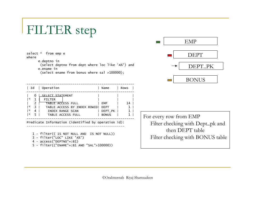
select * from emp e where e.deptno in (select deptno from dept where loc like 'A%') and e.ename in (select ename from bonus where sal >100000);

-------------------------------------------------------- | Id | Operation | Name | Rows | -------------------------------------------------------- | 0 | SELECT STATEMENT | | | |* 1 | FILTER | | | | 2 | TABLE ACCESS FULL | EMP | 14 | |* 3 | TABLE ACCESS BY INDEX ROWID| DEPT | 1 | |* 4 | INDEX RANGE SCAN | DEPT_PK | 1 | |* 5 | TABLE ACCESS FULL | BONUS | 1 | -------------------------------------------------------- Predicate Information (identified by operation id): ---------------------------------------------------

1 - filter(( IS NOT NULL AND IS NOT NULL)) 3 - filter("LOC" LIKE 'A%') 4 - access("DEPTNO"=:B1) 5 - filter(("ENAME"=:B1 AND "SAL">100000))

FILTER step EMP

DEPT

DEPT_PK

BONUS

For every row from EMP Filter checking with Dept_pk and

then DEPT table Filter checking with BONUS table


Subquery unnesting

Subquery unnesting is an optimization step in which sub queries are unnested to a join.

select * from emp e where

e.deptno in (select deptno from dept where loc like 'A%') and

e.ename in (select ename from bonus where sal >100000);

----------------------------------------------------------------------------- | Id | Operation | Name | Rows | Bytes | Cost (%CPU)| Time |

----------------------------------------------------------------------------- | 0 | SELECT STATEMENT | | | | 7 (100)| | |* 1 | HASH JOIN SEMI | | 5 | 675 | 7 (15)| 00:00:01 |

|* 2 | HASH JOIN SEMI | | 5 | 575 | 5 (20)| 00:00:01 | | 3 | TABLE ACCESS FULL| EMP | 14 | 1316 | 2 (0)| 00:00:01 |

|* 4 | TABLE ACCESS FULL| DEPT | 1 | 21 | 2 (0)| 00:00:01 | |* 5 | TABLE ACCESS FULL | BONUS | 1 | 20 | 2 (0)| 00:00:01 | -----------------------------------------------------------------------------


Summary

  There are different types of join techniques.

  There are no one join techniques superior to other join technique. If that is the case, Oracle product would not choose inferior techniques.

  Choosing a join method suitable for the SQL statement is also a necessary step of tuning that statement.


Common problem areas in an execution plan.


Identify plan issues

  There are couple of clues in the execution plan that can give you a hint about the root cause.

  Following few slides details these clues. But, this is not a complete list.

  It is probably a better idea to test your theory   by rewriting the query   by adjusting the execution plan with hints   by testing with a different database or different set of data.


Cardinality feedback

  Cardinality is the measure of optimizer estimate for the number of rows returned in a step.

Select * from table (dbms_xplan.display); --------------------------------------------------------------------------------------------- | Id | Operation | Name | Rows | Bytes | Cost (%CPU)| --------------------------------------------------------------------------------------------- | 0 | SELECT STATEMENT | | 1 | 214 | 9 (23)| | 1 | SORT ORDER BY | | 1 | 214 | 9 (23)| |* 2 | TABLE ACCESS BY INDEX ROWID | RCV_STAGING_LINES | 1 | 155 | 4 (25)| | 3 | NESTED LOOPS | | 1 | 214 | 8 (13)| |* 4 | TABLE ACCESS BY INDEX ROWID| RCV_STAGING_HEADERS | 1 | 59 | 5 (20)| |* 5 | INDEX RANGE SCAN | RCV_STAGING_HEADERS_N5 | 20 | | 4 (25)| |* 6 | INDEX RANGE SCAN | RCV_STAGING_LINES_N3 | 1 | | 3 (34)| ----------------------------------------------------------------------------------------------

  In this case, optimizer estimates that step 6, accessing through index returned 20 rows.

  Step 4 reduced that just one row. So, you need to investigate to see why there is many rows estimated to be returned in that step.


Cardinality feedback (2)

  Match the run time statistics and the execution plan. Identify the difference in the estimate and actual statistics.

--------------------------------------------------------------------------------------------- | Id | Operation | Name | Rows | Bytes | Cost (%CPU)| --------------------------------------------------------------------------------------------- | 0 | SELECT STATEMENT | | 1 | 214 | 9 (23)| | 1 | SORT ORDER BY | | 1 | 214 | 9 (23)| |* 2 | TABLE ACCESS BY INDEX ROWID | RCV_STAGING_LINES | 1 | 155 | 4 (25)| | 3 | NESTED LOOPS | | 1 | 214 | 8 (13)| |* 4 | TABLE ACCESS BY INDEX ROWID| RCV_STAGING_HEADERS | 1 | 59 | 5 (20)| |* 5 | INDEX RANGE SCAN | RCV_STAGING_HEADERS_N5 | 20 | | 4 (25)| |* 6 | INDEX RANGE SCAN | RCV_STAGING_LINES_N3 | 1 | | 3 (34)| ----------------------------------------------------------------------------------------------

Rows Row Source Operation ------- --------------------------------------------------- 0 TABLE ACCESS BY INDEX ROWID RCV_STAGING_LINES 0 NESTED LOOPS 0 NESTED LOOPS 14 TABLE ACCESS BY INDEX ROWID RCV_STAGING_HEADERS 2608158 INDEX RANGE SCAN RCV_STAGING_HEADERS_N5 14 INDEX RANGE SCAN RCV_STAGING_LINES_N3

  In this example below, optimizer estimates are off, especially for step 5..


Leading table   In most cases, if the optimizer chooses correct starting table, then the performance of that SQL statement will be tolerable.

Rows Row Source Operation ------- ---------------------------------------------------

1000 SORT GROUP BY (cr=33914438 r=0 w=0 time=386540124 us) 1000 NESTED LOOPS (cr=33914438 r=0 w=0 time=386162642 us)

16540500 TABLE ACCESS BY INDEX ROWID OBJ#(38049)(cr=831438 r=0 w=0 time=146900634us ) 16540500 INDEX RANGE SCAN OBJ#(149297) (cr=154584 r=0 w=0 time=25026467 us)(obj 149297) 1000 INDEX RANGE SCAN OBJ#(5743997) (cr=33083000 r=0 w=0 time=202120686 us)(obj 5743997)

  Try to understand why the optimizer did not chose correct starting table.

  In this example, leading table is chosen unwisely.


Leading table (2)

  With a leading hint, SQL was tuned to start from object id 5743997, which was a temporary table.

Rows Row Source Operation ------- ---------------------------------------------------

0 SORT GROUP BY (cr=3067 r=0 w=0 time=38663 us) 0 TABLE ACCESS BY INDEX ROWID OBJ#(38049) (cr=3067 r=0 w=0 time=26516 us)

1000 NESTED LOOPS (cr=3067 r=0 w=0 time=24509 us) 0 INDEX RANGE SCAN OBJ#(5743997) (cr=3067 r=0 w=0 time=23379 us)(object id 5743997) 0 INDEX RANGE SCAN OBJ#(1606420) (object id 1606420)

  Performance of that SQL is much better with temporary table chosen as a leading table.


Writing optimal SQL


Avoid loop based processing FOR c1 in cursor_c1 LOOP -- v_commit_count := v_commit_count + 1;

INSERT INTO RECS_TEMP VALUES (c1.join_record , -- JOIN_RECORD c1.location , -- LOCATION c1.item_number , -- ITEM_NUMBER c1.wh_report_group , -- WH_REPORT_GROUP c1.po_number , -- PO_NUMBER

... ); IF v_commit_count = 100000 THEN COMMIT; v_loop_counter := v_loop_counter + 1; v_commit_count := 0; END IF; -- END LOOP;

For each row from outer cursor..

Insert a row in to the table.

Commit after every 100K rows.


Loop based processing

Send SQL

Execute SQL

Fetch first row

Return row

Insert one row

Insert and send status

Fetch next row

Return row

Insert next row

PL/SQL SQL

Insert and send status

This is known as “chatty” application and encounters much performance issues…


Think in terms of set

  SQL is a set language. SQL is optimized to work as a set language.

  Avoid row-by-row processing if possible.

  In some cases, Loops are unavoidable.


Rewritten loop INSERT INTO RECS_TEMP (col1, col2, col3…coln) SELECT join_record , -- JOIN_RECORD location , -- LOCATION item_number , -- ITEM_NUMBER report_group , -- WH_REPORT_GROUP po_number , -- PO_NUMBER ... FROM c1_cust_view t WHERE t.asset_id BETWEEN p_min_val AND p_max_val GROUP BY t.location||'.'||t.item_number, t.location, t.item_number, t.wh_report_group, t.po_number, t.loc_company, -- t.loc_company, t.location_type, t.asset_id, t.book_type_code, t.asset_major_category, t.asset_minor_category ;

One simple insert statement inserting all necessary rows.


Few guidelines…

  Use direct SQL statements.

  If PL/SQL loop can’t be avoided use array based processing.

  bulk bind, bulk fetch, bulk insert etc.

  If another host language such as ‘C’ or java, use arrays and host language facilities to reduce round trip network calls between client and the database.


Transformed predicates

  Transformed predicates means that optimizer will not be able to choose index based execution plan.

-------------------------------------------- | Id | Operation | Name | E-Rows | --------------------------------------------

|* 1 | HASH JOIN | | 1 | |* 2 | TABLE ACCESS FULL| DEPT | 1 |

| 3 | TABLE ACCESS FULL| EMP | 14 | --------------------------------------------


1 - access(SUBSTR(TO_CHAR("E"."DEPTNO"),1,10)=SUBSTR(TO_CHAR("D"."DEPTNO"),1,10)) 2 - filter("D"."DNAME" LIKE 'A%')

select ename from emp e, dept d where substr(to_char(e.deptno),1,10)= substr(to_char(d.deptno),1,10) and d.dname like 'A%'


Join predicates

  Avoid function calls and tranformed predicates in the join predicates.

-------------------------------------------- | Id | Operation | Name | E-Rows | -------------------------------------------- |* 1 | HASH JOIN | | 19 | | 2 | TABLE ACCESS FULL| DEPT | 4 | | 3 | TABLE ACCESS FULL| EMP | 14 | --------------------------------------------

Predicate Information (identified by operation id): --------------------------------------------------- 1 - access("E"."DEPTNO"=NVL("D"."DEPTNO",10))

select ename from emp e, dept d where e.deptno = nvl(d.deptno,10);


Function rewritten   Rewriting function call might make SQL complex, but perform better.

----------------------------------------------- | Id | Operation | Name | E-Rows |

----------------------------------------------- | 1 | NESTED LOOPS | | 14 |

| 2 | TABLE ACCESS FULL| EMP | 14 | |* 3 | INDEX RANGE SCAN | DEPT_PK | 1 | -----------------------------------------------

Predicate Information (identified by operation id):

---------------------------------------------------

3 - access("E"."DEPTNO"="D"."DEPTNO")

filter(("D"."DEPTNO" IS NOT NULL OR ("D"."DEPTNO" IS NULL AND “E"."DEPTNO"=10)))

select ename from emp e, dept d where (e.deptno =d.deptno and d.deptno is not null) or (e.deptno =d.deptno and d.deptno is null and e.deptno=10);


Implicit transformation

  Implicit transformation also can lead to poor execution plan. Column deptno2 is a character column and to_number function must be applied.

-------------------------------------------- | Id | Operation | Name | E-Rows |

-------------------------------------------- |* 1 | HASH JOIN | | 4 |

|* 2 | TABLE ACCESS FULL| DEPT | 1 | | 3 | TABLE ACCESS FULL| EMP | 14 | --------------------------------------------


1 - access("D"."DEPTNO"=TO_NUMBER("E"."DEPTNO2")) 2 - filter("DNAME" LIKE 'A%')

select ename from emp e, dept d where e.deptno2 =d.deptno and dname like 'A%'


Conversion

  You can apply filter predicates in the correct side of equality join to use index access path.

------------------------------------------------------- | Id | Operation | Name | E-Rows |

------------------------------------------------------- | 1 | TABLE ACCESS BY INDEX ROWID| EMP | 5 |

| 2 | NESTED LOOPS | | 5 | |* 3 | TABLE ACCESS FULL | DEPT | 1 | |* 4 | INDEX RANGE SCAN | EMP_C1 | 5 |

------------------------------------------------------- Predicate Information (identified by operation id):

--------------------------------------------------- 3 - filter("DNAME" LIKE 'A%') 4 - access("E"."DEPTNO2"=TO_CHAR("D"."DEPTNO"))

select ename from emp e, dept d where e.deptno2 =to_char(d.deptno) and dname like 'A%‘;


Excessive revisits   Avoid revisiting data.

Select count(*) from employees where department=‘ACCOUNTING’;

Select count(*) from employees where department=‘FINANCE’ or ‘IT’;

Select count(*) from employees;

  Above SQL statement can be rewritten as: Employees accessed just once.

Select

count( case when department =‘ACCOUNTING’ then 1 else 0 end ) acct_cnt,

count( case when department =‘FINANCE’ or department=‘IT’ then 1 else 0 end) fin_it_cnt,

count(*)

From employees;


Full table scan

  Not all full table scans (FTS) are bad.

  In some cases, FTS is cheaper than performing index and then table block access.

  Especially, if the driving table has higher number of rows and the inner table has few rows, then it may be better to do FTS.

Rows Row Source Operation ------- --------------------------------------------------- 43935 TABLE ACCESS BY INDEX ROWID FA_METHODS (cr=743619 pr=272870 pw=0 time=826315272 us) 87870 NESTED LOOPS (cr=738078 pr=272865 pw=0 time=825760138 us) 43935 NESTED LOOPS (cr=644350 pr=272865 pw=0 time=809397304 us) ... 43935 INDEX RANGE SCAN FA_METHODS_U2 (cr=93728 pr=0 pw=0 time=16211647 us)(object id 32589)

FA_METHODS is a small table with 500 rows. But, outer table returned 43,000 times and FA_METHODS accessed 43,000 times.


FTS and Hash join

  FTS combined with hash join will perform better in this case.

Rows Row Source Operation ------- --------------------------------------------------- 30076 HASH JOIN (cr=4250352 pr=1043030 pw=0 time=1887152322 us) 411487 NESTED LOOPS (cr=4250335 pr=1043019 pw=0 time=2396907676 us) 411487 NESTED LOOPS (cr=3015121 pr=861281 pw=0 time=2136848154 us) ... 580 TABLE ACCESS FULL FA_METHODS (cr=17 pr=11 pw=0 time=21346 us)

411K rows joined with 580 tables. Access to FA_METHODS took only 21 milli-seconds.


NULL

  Certain constructs with ‘IS NULL’ predicates may not use index.

  NULL values are not stored in single column indices and so, index may not be usable.

  Even if you have index on deptno column, in the example below, that index can not be used. This query is very typical in manufacturing applications.

Select * from emp where deptno is null;

  One way to use index and improve performance is to use case statement and a function based index.

Create index emp_f1 on emp ( case when deptno is null then ‘X’ else null end);

Select * from emp where ( case when deptno is null then ‘X’ else null end) is not null;


Use Bind variables

  Use of bind variables leads to sharable SQL statement.

  Hard parsing a SQL statement is an expensive operation and lead to poor application scalability.

Select ename from emp where first_name=:B1;

  Handful of exceptions.

  SQL statements accessing columns with very low cardinality. Optimizer can determine the cardinality correctly with a literal value.

select * from transaction_interface where processed =‘N’;

  Data ware house queries which generally are not executed repeatedly.


Hints


HINTS

  Hints are directive to the optimizer and almost always honored by the optimizer.

  Hints are not honored only if the hints are inconsistent with itself or another hint.

  Avoid hints, if possible. Many software upgrade performance issues that I have seen is due to hints(bad).

  In some cases, hints are necessary evils


ORDERED

  ORDERED hint Dictates optimizer an exact sequence of tables to join [ top to bottom or L->R canonically speaking].

Select …

From t1,

t2,

t3,

t4

t1 t2 t3 t4


ORDERED

explain plan for select /*+ ORDERED */

t1.n1, t2.n2 from t_large2 t2,

t_large t1 where t1.n1 = t2.n1 and t2.n2=100 /

-------------------------------------------------------------------------------------

| Id | Operation | Name | Rows | Bytes | Cost (%CPU)| Time | ------------------------------------------------------------------------------------- | 0 | SELECT STATEMENT | | 1 | 13 | 1401 (5)| 00:00:08 |

| 1 | NESTED LOOPS | | 1 | 13 | 1401 (5)| 00:00:08 | |* 2 | INDEX FAST FULL SCAN| T_LARGE2_N2 | 1 | 8 | 1399 (6)| 00:00:07 |

|* 3 | INDEX RANGE SCAN | T_LARGE_N1 | 1 | 5 | 2 (0)| 00:00:01 | -------------------------------------------------------------------------------------

t2 t1

t1.n1=t2.n1

n2=100


ORDERED

  Later developer added another table to the join..

explain plan for select /*+ ORDERED */


t_large2 t2, t_large t1

where t1.n1 = t2.n1 and t2.n2=100

and t1.n1=t3.n1 /

t2 t1

t1.n1=t2.n1

n1=100

t3

----------------------------------------------------------------------------------------------- | Id | Operation | Name | Rows | Bytes |TempSpc| Cost (%CPU)| Time | ----------------------------------------------------------------------------------------------- | 0 | SELECT STATEMENT | | 1 | 18 | | 1397M (6)|999:59:59 | |* 1 | HASH JOIN | | 1 | 18 | 11M| 1397M (6)|999:59:59 | | 2 | MERGE JOIN CARTESIAN | | 499K| 6345K| | 1397M (6)|999:59:59 | | 3 | INDEX FAST FULL SCAN | T_LARGE3_N1 | 999K| 4880K| | 1161 (4)| 00:00:06 | | 4 | BUFFER SORT | | 1 | 8 | | 1397M (6)|999:59:59 | |* 5 | INDEX FAST FULL SCAN| T_LARGE2_N2 | 1 | 8 | | 1398 (6)| 00:00:07 | | 6 | INDEX FAST FULL SCAN | T_LARGE_N1 | 1100K| 5371K| | 1176 (5)| 00:00:06 | -----------------------------------------------------------------------------------------------

Optimizer did exactly what it is told to!


Ordered & leading

explain plan for select /*+ leading (t2) */


t_large2 t2, t_large t1

where t1.n1 = t2.n1 and t2.n2=100

and t1.n1=t3.n1 /

t2 t1

t1.n1=t2.n1

n1=100

t3

--------------------------------------------------------------------------------------

| Id | Operation | Name | Rows | Bytes | Cost (%CPU)| Time | --------------------------------------------------------------------------------------

| 0 | SELECT STATEMENT | | 1 | 18 | 1403 (5)| 00:00:08 | | 1 | NESTED LOOPS | | 1 | 18 | 1403 (5)| 00:00:08 | | 2 | NESTED LOOPS | | 1 | 13 | 1401 (5)| 00:00:08 |

|* 3 | INDEX FAST FULL SCAN| T_LARGE2_N2 | 1 | 8 | 1399 (6)| 00:00:07 | |* 4 | INDEX RANGE SCAN | T_LARGE_N1 | 1 | 5 | 2 (0)| 00:00:01 |

|* 5 | INDEX RANGE SCAN | T_LARGE3_N1 | 1 | 5 | 2 (0)| 00:00:01 |

If you must, use leading instead of ordered..


Indexing, partitioning and more


Choose index wisely

explain plan for select * from emp where ename ='JACOB' and hiredate > sysdate-365;

-------------------------------------------------------------------------- | Id | Operation | Name | Rows | Bytes | Cost (%CPU)| Time |

-------------------------------------------------------------------------- | 0 | SELECT STATEMENT | | 1 | 40 | 2 (0)| 00:00:01 | |* 1 | TABLE ACCESS FULL| EMP | 1 | 40 | 2 (0)| 00:00:01 |

--------------------------------------------------------------------------


1 - filter("ENAME"='JACOB' AND "HIREDATE">SYSDATE@!-365)

  Leading column of indices should contain most common predicates.

  In the example above, creating an index on ename would be helpful.


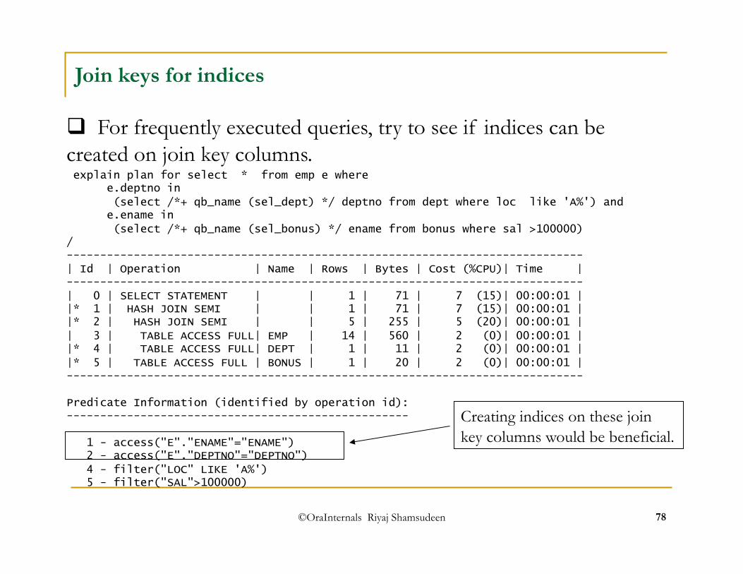
Join keys for indices

explain plan for select * from emp e where e.deptno in

(select /*+ qb_name (sel_dept) */ deptno from dept where loc like 'A%') and e.ename in

(select /*+ qb_name (sel_bonus) */ ename from bonus where sal >100000) / -----------------------------------------------------------------------------

| Id | Operation | Name | Rows | Bytes | Cost (%CPU)| Time | -----------------------------------------------------------------------------

| 0 | SELECT STATEMENT | | 1 | 71 | 7 (15)| 00:00:01 | |* 1 | HASH JOIN SEMI | | 1 | 71 | 7 (15)| 00:00:01 | |* 2 | HASH JOIN SEMI | | 5 | 255 | 5 (20)| 00:00:01 |

| 3 | TABLE ACCESS FULL| EMP | 14 | 560 | 2 (0)| 00:00:01 | |* 4 | TABLE ACCESS FULL| DEPT | 1 | 11 | 2 (0)| 00:00:01 |

|* 5 | TABLE ACCESS FULL | BONUS | 1 | 20 | 2 (0)| 00:00:01 | -----------------------------------------------------------------------------


1 - access("E"."ENAME"="ENAME") 2 - access("E"."DEPTNO"="DEPTNO")

4 - filter("LOC" LIKE 'A%') 5 - filter("SAL">100000)

  For frequently executed queries, try to see if indices can be created on join key columns.

Creating indices on these join key columns would be beneficial.


Column selectivity

Table Number Empty Average Name of Rows Blocks Blocks Space --------------- -------------- ------------ ------------ ------- MTL_MATERIAL_TR 170,392,833 13,551,182 0 0 ANSACTIONS

Column Column Distinct Name Details Values ------------------------- ------------------------ -------------- ... ORGANIZATION_ID NUMBER(22) NOT NULL 2,589 INVENTORY_ITEM_ID NUMBER(22) NOT NULL 7,703 ...

  Selectivity of the column indices how many rows will be returned from the table.

  For organization_id alone in the index, approximately, each key entry will return 65,814 rows: 170392833/2589 = 65814

  For organization_id , inventory_item_id; Each combination of key entry will return just 8 rows: 170392833/(2589*7703) = 8

Where organization_id = :b1 and inventory_item_id=:b2


Avoid updated columns

  Do not index columns that are updated heavily.

  Updates to indexed columns are equivalent of a delete and insert at index level.

 In this example, quantity is a good candidate column, but updated heavily. So, that column should not be indexed. explain plan for Select attribute1, quantity, quantity_cancelled, quantity_delivered from

PO_REQUISITION_LINES_ALL where item_id=:b1 and quantity >100 /

------------------------------------------------------------------------ | Id | Operation | Name | Rows | ------------------------------------------------------------------------

| 0 | SELECT STATEMENT | | 1545 | |* 1 | TABLE ACCESS BY INDEX ROWID| PO_REQUISITION_LINES_ALL | 1545 |

|* 2 | INDEX RANGE SCAN | PO_REQUISITION_LINES_N7 | 1545 | ------------------------------------------------------------------------

1 - filter("QUANTITY">100) 2 - access("ITEM_ID"=TO_NUMBER(:B1))


Other index types

  There are more index types then just b-tree indices

  bitmap indices

  Index organized tables

  Partitioned indices etc.

  Consider activity while choosing index. For example, bitmap indices are useful only for read only tables (like data warehouse tables).

  Index Organized tables are suitable for tables which are accessed just using just leading columns of the table.


Partitioning

  Consider table partitioning for many reasons:

  Easy archiving of data. Example: gl_balances on period_name

  Performance of table scan. For example, report SQLs accessing just last period on gl_balances table.

  Partition to improve scalability of the table. Hash partition the table inserted aggressively with primary key/unique keys.


Unscalable index

Root block

Branch block

Leaf blocks

Primary key index on line_id

Ses 1: inserting value of 10000




All sessions inserting into a leaf block.


Hash partitioning

Root block

Branch block

Leaf blocks

Primary key index on line_id

All sessions inserting into a leaf block.

Root block

Branch block

Ses 1: inserting value of 10000 Ses 2: inserting value of 10001

Ses 3: inserting value of 10002 Ses 4: inserting value of 10003


SQL tuning advisor


10g : SQL tuning advisor

  SQL tuning advisor available in 10g is very useful.

  This tool must be used as first level of testing so that basic issues can be avoided.

  dbms_sqltune package is called to access tuning advisor:

  Create tuning task

  Execute tuning task

  See the report.

For complex SQLs, it might not be very helpful, but worth a try.


Step 1: Create tuning task

DECLARE my_task_name VARCHAR2(30); my_sqltext CLOB; BEGIN my_sqltext := q'[select ename from demo1.emp e, demo1.dept d where e.deptno2 =d.deptno and dname like 'A%' ]'; my_task_name := DBMS_SQLTUNE.CREATE_TUNING_TASK( sql_text => my_sqltext, user_name => user, scope => 'COMPREHENSIVE', time_limit => 60, task_name => 'RS_TEST_SQL_1', description => 'Task to tune a query '); END; / Time limit for this task Unique task name


Step 2: Execute tuning task

Begin dbms_sqltune.Execute_tuning_task (task_name => 'RS_TEST_SQL_1'); end; /


Step 3: Report tuning task set longchunksize 10000 set linesize 200 set pagesize 200 Set long 10000 select * from dba_advisor_log where task_name='RS_TEST_SQL_1'; select dbms_sqltune.report_tuning_task('RS_TEST_SQL_1') from dual;

----------------------- GENERAL INFORMATION SECTION ------------------------------------------------------------------------------- Tuning Task Name : RS_TEST_SQL_1 Tuning Task Owner : SYS Scope : COMPREHENSIVE Time Limit(seconds) : 60 Completion Status : COMPLETED Started at : 01/20/2010 21:57:44 Completed at : 01/20/2010 21:57:45 Number of Statistic Findings : 2

------------------------------------------------------------------------------- Schema Name: SYS SQL ID : 9vgx715q6ng77 SQL Text : select ename from demo1.emp e, demo1.dept d where e.deptno2 =d.deptno and dname like 'A%'

..continued on next page


Recommendations… ------------------------------------------------------------------------------- FINDINGS SECTION (2 findings) -------------------------------------------------------------------------------

1- Statistics Finding --------------------- Table "DEMO1"."DEPT" was not analyzed.

Recommendation -------------- - Consider collecting optimizer statistics for this table. execute dbms_stats.gather_table_stats(ownname => 'DEMO1', tabname => 'DEPT', estimate_percent => DBMS_STATS.AUTO_SAMPLE_SIZE, method_opt => 'FOR ALL COLUMNS SIZE AUTO');

Rationale --------- The optimizer requires up-to-date statistics for the table in order to select a good execution plan.

2- Statistics Finding --------------------- Table "DEMO1"."EMP" was not analyzed.

Recommendation -------------- - Consider collecting optimizer statistics for this table. execute dbms_stats.gather_table_stats(ownname => 'DEMO1', tabname => 'EMP', estimate_percent => DBMS_STATS.AUTO_SAMPLE_SIZE, method_opt => 'FOR ALL COLUMNS SIZE AUTO'); …

By Riyaj Shamsudeen - Oracle database internals by Riyaj · PDF file©OraInternals Riyaj...

Documents

Transcript of By Riyaj Shamsudeen - Oracle database internals by Riyaj · PDF file©OraInternals Riyaj...