Anyons and Lowest Landau Level Anyons - · PDF file · 2007-12-21Anyons and Lowest...

Seminaire Poincare XI (2007) 77 – 107 Seminaire Poincare

Anyons and Lowest Landau Level Anyons

Stephane Ouvry

Laboratoire de Physique Theorique et Modeles Statistiques,Universite Paris-SudCNRS UMR 862691405 Orsay Cedex, France

Abstract. Intermediate statistics interpolating from Bose statistics to Fermistatistics are allowed in two dimensions. This is due to the particular topol-ogy of the two dimensional configuration space of identical particles, leadingto non trivial braiding of particles around each other. One arrives at quantummany-body states with a multivalued phase factor, which encodes the anyonicnature of particle windings. Bosons and fermions appear as two limiting cases.Gauging away the phase leads to the so-called anyon model, where the chargeof each particle interacts ”a la Aharonov-Bohm” with the fluxes carried by theother particles. The multivaluedness of the wave function has been traded off fortopological interactions between ordinary particles. An alternative Lagrangianformulation uses a topological Chern-Simons term in 2+1 dimensions. Takinginto account the short distance repulsion between particles leads to an Hamil-tonian well defined in perturbation theory, where all perturbative divergenceshave disappeared. Together with numerical and semi-classical studies, pertur-bation theory is a basic analytical tool at disposal to study the model, sincefinding the exact N -body spectrum seems out of reach (except in the 2-bodycase which is solvable, or for particular classes of N -body eigenstates whichgeneralize some 2-body eigenstates). However, a simplification arises when theanyons are coupled to an external homogeneous magnetic field. In the case ofa strong field, by projecting the system on its lowest Landau level (LLL, thusthe LLL-anyon model), the anyon model becomes solvable, i.e. the classes of ex-act eigenstates alluded to above provide for a complete interpolation from theLLL-Bose spectrum to the LLL-Fermi spectrum. Being a solvable model allowsfor an explicit knowledge of the equation of state and of the mean occupationnumber in the LLL, which do indeed interpolate from the Bose to the Fermicases. It also provides for a combinatorial interpretation of LLL-anyon braidingstatistics in terms of occupation of single particle states. The LLL-anyon modelmight also be relevant experimentally: a gas of electrons in a strong magneticfield is known to exhibit a quantized Hall conductance, leading to the integerand fractional quantum Hall effects. Haldane/exclusion statistics, introduced todescribe FQHE edge excitations, is a priori different from anyon statistics, sinceit is not defined by braiding considerations, but rather by counting argumentsin the space of available states. However, it has been shown to lead to the samekind of thermodynamics as the LLL-anyon thermodynamics (or, in other words,the LLL-anyon model is a microscopic quantum mechanical realization of Hal-dane’s statistics). The one dimensional Calogero model is also shown to havethe same kind of thermodynamics as the LLL-anyons thermodynamics. This isnot a coincidence: the LLL-anyon model and the Calogero model are intimately

78 S. Ouvry Seminaire Poincare

related, the latter being a particular limit of the former. Finally, on the purelycombinatorial side, the minimal difference partition problem -partition of in-tegers with minimal difference constraints on their parts- can also be mappedon an abstract exclusion statistics model with a constant one-body density ofstates, which is neither the LLL-anyon model nor the Calogero model.

1 Introduction

Quantum statistics, which is concerned with quantum many-body wavefunctions ofidentical particles, has a long history going back to Bose and Fermi. The conceptof statistics originates at the classical level in the Gibbs paradox, which is solvedby means of the indiscernability postulate for identical particles. At the quantumlevel, the usual reasoning shows that only two types of statistics can exist, bosonicor fermionic. Indeed, since

• interchanging the positions of two identical particles can onlyamount to multiplying their 2-body wavefunction by a phase factor,

• a double exchange puts back the particles at their original position,

• and one usually insists on the univaluedness of the wavefunction,

this phase factor can be only 1 (boson) or -1 (fermion).However, non trivial phase factor should be possible, since wavefunctions are

anyway defined up to a phase. The configuration space of two, or more generally, Nidentical particles has to be defined cautiously [1]: denoting by C the configurationspace of a single particle (C = R2 for particles in the two-dimensional plane, d = 2),the configuration space of N particles should be of the type CN/SN , where C ∗C ∗...∗C = CN and SN is the permutation group for N identical particles. Quotientingby SN takes into account the identity of the particles which implies that one cannotdistinguish between two configurations related by an operation of the permutationgroup. One should also subtract from CN the diagonal of the configuration spaceDN ,i.e. any configurations where two or more particles coincide. The reason is, havingin mind Fermi statistics, that the Pauli exclusion principle should be enforced insome way. A more precise argument is to have a valid classification of paths in theN -particle configuration space, which would be ambiguous if two or more particlescoinciding at some time is allowed (since they are identical, did they cross eachother, or did they scatter off each other ?). It follows that the configuration spaceof N identical particles should be

CN =CN −DN

SN(1)

Note that on this configuration space, a fermionic wavefunction is multivalued(two values 1 and -1), so there is no reason not to allow more general multivaluedness.Here come some topological arguments, which allow to distinguish between d = 2and d > 2, and, as we will see later, which can be related to spin considerations.In 2 dimensions, CN is multiply connected and its topology is non trivial: it isnot possible to shrink a path of a particle encircling another particle, due to thetopological obstruction materialized by the latter. It follows that CN is multiplyconnected. This is not the case in dimensions higher than 2, where CN is simply

Vol. XI, 2007 Anyons and Lowest Landau Level Anyons 79

connected, meaning that all paths made by a particle can be continuously deformedinto each other, i.e. one cannot distinguish the interior from the exterior of a closedpath of a particle around other particles.

These arguments imply that the equivalent classes of paths (first homotopygroup) in CN are, when d = 2, in one-to-one correspondence with the elements ofthe braid group

Π1(CN) = BN (2)

whereas, when d > 2, they are in one-to-one correspondence with the elements ofthe permutation group

Π1(CN) = SN (3)

The braid group generators σi interchange the position of particle i with particlei + 1. This operation can be made in an anti-clockwise manner (σi) or a clockwisemanner (σ−1

i ). Each braiding of N particles consists of a sequence of interchanges ofpairs of neighboring particles via the σi’s and the σ−1

i ’s, with i = 1, 2, ..., N −1. Thebraid group relations list the equivalent braiding, i.e. braiding that can be continu-ously deformed one into the other without encountering a topological obstruction

σiσi+1σi = σi+1σiσi+1; σiσj = σjσi when |i− j| > 2 (4)

Figure 1: The braid group generators and their defining relations.

Saying that d = 2 is different from d > 2 is nothing but recognizing thatσi 6= σ−1

i when d = 2, whereas σi = σ−1i when d > 2 (σi can be continuously


deformed into σ−1i when particles i and i+1 are not stuck in a plane). It follows that

when d > 2, the braid generators σi’s defined by (4) with the additional constraintσi = σ−1

i are the permutation group generators.Note also that the d = 2 paradigm, σi 6= σ−1

i , hints at an orientation of theplane, a hallmark of the presence of some sort of magnetic field. This point willbecome apparent in the Aharonov-Bohm formulation of the anyon model.

The fact that CN is multiply connected when d = 2 and not when d > 2 can alsobe related to the rotation group O(d), and thus to some spin-statistics considerations[2]. When d > 2, the rotation group is doubly connected, [Π1(O(d)) = Z2], itsuniversal covering, for example when d = 3, is SU(2), which allows for either integeror half integer angular momentum states, that is to say either single valued or doublevalued representations of the rotation group. On the other hand, when d = 2, therotation group is abelian and infinitely connected [Π1(O(2)) = Z], its universalcovering is the real line, that is to say arbitrary angular momenta are possible,and therefore multivalued representations. One can see here a hint about the spin-statistics connection, where statistics and spin are trivial (Bose-Fermi statistics,integer-half integer spin) when d > 2, and not when d = 2.

Let us consider the simple one-dimensional irreducible representation of thebraid group, which amounts to a common phase factor exp(−iπα) for each gen-erator σ (and thus exp(iπα) to σ−1). It means that a non trivial phase has beenassociated with the winding of particle i around particle i + 1. Higher dimensionalrepresentations (quantum vector states) are possible -one speaks of non abeliananyons, in that case not only a non trivial phase materializes during a winding,but also the direction of the vector state in the Hilbert space is affected- but theywill not be discussed here (even though they might play a role in the discussion ofcertain FQHE fractions [3], and, in a quite different perspective, in the definition oftopologically protected fault-tolerant quantum computers [4]).

Clearly, when d > 2, σi = σ−1i implies α = 0 or α = 1, i.e. Bose or Fermi

statistics (an interchange leaves the wavefunction unchanged or affected by a minussign).

From now on let us concentrate on d = 2 and denote the free many-bodywavefunction of N identical particles by ψ′(~r1, ~r2, ..., ~rN). Indeed, statistics shouldbe defined for free particles with Hamiltonian

H ′N =

N∑

i=1

~p2i

2m(5)

and special boundary conditions on the wavefunction, as in the Bose case (symmetricboundary condition) and the Fermi case (antisymmetric boundary condition). Asalready said, ψ′(~r1, ~r2, ..., ~rN) is affected by a phase exp(−iπα) when particles i andi+1 are interchanged: one can encode this non trivial exchange property by defining

ψ′(~r1, ~r2, ..., ~rN) = exp(−iα∑

i<j

θij)ψ(~r1, ~r2, ..., ~rN) (6)

where ψ(~r1, ~r2, ..., ~rN) is a regular wavefunction, say bosonic by convention, and θij

is the angle between the vector ~rj−~ri ≡ ~rij and a fixed direction in the plane. Indeedinterchanging i with j amounts to θij → θij ± π, which altogether with the bosonicsymmetry of ψ(~r1, ~r2, ..., ~rN), leads to

ψ′(~r1, ~r2, ...~rj, ...~ri, ..., ~rN) = exp(∓iπα)ψ′(~r1, ~r2, ...~ri, ...~rj, ..., ~rN) (7)


By the above bosonic convention for ψ(~r1, ~r2, ..., ~rN), the statistical parameterα even (odd) integer corresponds to Bose (Fermi) statistics. It is defined modulo 2,since two quanta of flux can always be gauged away by a regular gauge transfor-mation while preserving the symmetry of the wavefunctions in the Bose or Fermisystems. Indeed, (6) can be interpreted as a gauge transformation. Let us computethe resulting Hamiltonian HN acting on ψ(~r1, ~r2, ..., ~rN)

HN =N

∑

i=1

1

2m(~pi − ~A(~ri))

2 (8)

where

~A(~ri) = α~∂i(∑

k<l

θkl) = α∑

j,j 6=i

~k ∧ ~rij

r2ij

(9)

is the statistical potential vector associated with the multivalued phase (the gaugeparameter). The free multivalued wavefunction has beentraded off for a regular bosonic wavefunction with topological singular magneticinteractions. The statistical potential vector (9) can be viewed as the Aharonov-Bohm (A-B) potential vector that particle i carrying a charge e would feel due tothe flux tube φ carried by the other particles, with e and φ related to the statisti-cal parameter α by α = eφ/(2π) = φ/φ0 (φ0 = 2π/e is the flux quantum in units~ = 1). The resulting composite charge-flux picture is known under the name ofanyon model [5] since it describes particles with ”any” (any-on) statistics.

Figure 2: The two equivalent formulations of anyon statistics in terms, on the left, of a puncturedplane and, on the right, of usual bosonic particles interacting via topological A-B interactions.The loop of particle i around particle j cannot be continuously deformed to nothing due to thetopological obstruction materialized by the puncture at the location of particle j.

Computing the field strength one obtains

α

e~∂i ∧

∑

j,j 6=i

~k ∧ ~rij

r2ij

=2πα

e

∑

j,j 6=i

δ(~rij) (10)


meaning that each particle carries an infinite singular magnetic field with flux φ =2πα/e. The gauge transformation is singular since it does not preserve the fieldstrength (which vanishes in the multivalued gauge and is singular in the regulargauge). This is due to the singular behavior of the gauge parameter θij when particlei come close to particle j, thus the singular Dirac δ(~rij) function in the field strength.

It is not surprising that topological A-B interactions are at the heart of quan-tum statistics. In its original form, the A-B effect [6] consists in the phase shift inelectron interference due to the electromagnetic field, determined by the phase factorexp[(ie/~c)

∫

γAµdx

µ] along a closed curve γ passing through the beam along which

the field strength vanishes. This effect1 is counter-intuitive to the usual understand-ing that the influence of a classical electromagnetic field on a charged particle canonly occur through the local action of the field strength. In the context of quantumstatistics, it means that non trivial statistics arise through topological ”infinite”-distance interactions where no classical forces are present, as it should and as itis the case for Bose and Fermi statistics. Finally, singular magnetic fields give anorientation to the plane, which, as already said, shows up in σi 6= σ−1

i .All this can be equivalently restated in a Lagrange formulation which describes

again the system in topological terms, i.e. free particles minimally coupled to apotential vector whose dynamics is not Coulomb-like (Maxwell Lagrangian) butrather Chern-Simons [9]

LN =

N∑

i=1

(1

2m~v2

i + e( ~A(~ri)~vi − A0(~ri))) −κ

2ǫµνρ

∫

d2~rAµ∂νAρ (11)

with ǫµνρ the completely antisymmetric tensor (the metric is (+,−,−),xµ = (t, ~r) = (t, x, y), Aµ = (Ao, Ax, Ay), ǫ012 = ǫ012 = +1). Solving the Euler-Lagrange equations, in particular

∂σ δLN

δ(∂σA0)=δLN

δA0→ κ~∂ ∧ ~A(~r) = e

N∑

j=1

δ(~r − ~rj) (12)

leads to a magnetic field proportional to the density of particles in accordance with(10). Solving this last equation for ~A(~r) in the Coulomb gauge gives

~A(~r) =e

2πκ

N∑

j=1

~k ∧ (~r − ~rj)

(~r − ~rj)2(13)

in accordance with the A-B potential vector (9). Here again there is no Lorentz force,the potential vector is a pure gauge, the Chern-Simons term is metric independent,and the field strength is directly related to the matter current.

Coming back to the Hamiltonian formulation (8), one might ask how the ex-clusion of the diagonal of the configuration space materializes in the Hamiltonianformulation. One way to look at it is perturbation theory [10, 11]. Let us simplifythe problem by considering the standard A-B problem, i.e. a charged particle in theplane coupled to a flux tube at the origin with the Hamiltonian

H =1

2m(~p− α

~k ∧ ~rr2

)2 (14)

1The effect was first experimentally confirmed by R. G. Chambers [7], then by A. Tonomura [8].


Let us see what happens close to Bose statistics when α ≃ 0 (by periodicity αcan always been chosen in [−1/2,+1/2], an interval of length 1, since in the one-body case one quantum of flux can always be gauged away via a regular gaugetransformation). The A-B spectrum [6] is given by the Bessel functions

ψ(~r) = eilθJ|l−α|(kr) E =k2

2m(15)

with wavefunctions vanishing close to the origin r → 0 as J|l−α|(kr) ≃ r|l−α|. Whenthe angular momentum l 6= 0, this is the only possible locally square-integrablefunction. However, when l = 0, one could have as well J−|α|(kr) as a solution, since

it is still locally square-integrable even though it diverges at the origin as r−|α|. Inprinciple, the general solution in the l = 0 sector should be a linear combination ofJ|α|(kr) and J−|α|(kr), introducing an additional scale in the coefficient of the linearcombination [12]. Restricting the space of solutions as in (15), i.e. wavefunctionsvanishing at the origin, means that a short-range repulsive prescription has beenimposed on the behavior of the wavefunctions when the particle comes close tothe flux tube. One can give a more precise formulation of this fact by trying tocompute in perturbation theory the spectrum (15). Expanding the square in theHamiltonian (14), one finds that the α2/r2 term, which is as singular as the kineticterm, is divergent at second order in perturbation theory in the l = 0 sector. Itfollows that perturbation theory is not well defined in the problem as defined by theHamiltonian (14). A renormalization has to be implemented: one realizes that byadding the counterterm π|α|δ(~r) to (14), i.e. by considering

H =1

2m(~p− α

~k ∧ ~rr2

)2 +2π|α|m

δ(~r) (16)

the perturbative divergences due to the α2/r2 term are exactly cancelled by thosearising from the π|α|δ(~r) term at all orders in perturbation theory, giving back thespectrum (15). Physically, this repulsive δ contact term means that the particleis prevented from penetrating the core of the flux tube where the field strengthis infinite, thus the (at least) r|α| behavior when r → 0. Note that this has beenachieved without introducing any additional scale in the problem.

Clearly, in the N -body A-B anyon formulation of the model, the correspondingrenormalized Hamiltonian should read

HN =

N∑

i=1

1

2m(~pi − α

∑

j 6=i

~k ∧ ~rij

r2ij

)2 +2π|α|m

∑

i6=j

δ(~rij) (17)

realizing the quantum mechanical exclusion of the diagonal of the configurationspace in terms of contact repulsive interaction between particles. Note that the termπ|α|∑i6=j δ(~rij) in (17) can also be viewed [11] as the Pauli spin coupling of the spin

of the particles to the singular magnetic field (10) associated to the flux tubes.The anyon model defined in (17) is properly defined as far as short-distance con-

siderations are concerned. It is the interacting formulation for regular wavefunctionsof the free particles formulation for multivalued wavefunctions. Both HamiltoniansHN andH ′

N are equivalent, the former being more familiar in terms of usual quantummechanics, the latter more relevant to study braiding and winding properties.


The anyon model has been the subject of numerous studies in the eighties andthe nineties [13], some of them analytical, starting with the 2-body case which issolvable since its relative 2-body problem is the usual A-B problem (14) with aneven (Bose) angular momentum l. The exact solution [1, 5] for the relative 2-bodyproblem is given by (15), l being an even integer, therefore when α is odd, l − α isodd, corresponding to Fermi statistics (the periodicity α → α ± 2p is manifest inthe shift l → l − α). These studies were followed by the 3-body [14] and then theN -body problem [15]. Statistical mechanics was also considered (second virial coeffi-cient [16, 17], third virial coefficient [18]). However, it soon became apparent that acomplete N -body spectrum was out of reach, to the exception of particular classes ofexact eigenstates generalizing the 2-body eigenstates. Numerical [19] as well as semi-classical [20] studies were performed giving indications on the low energy N -bodyspectrum. A systematic study of the model was achieved at first [21] and at secondorder [22] in perturbation theory (at second order the complexity of the model showsup clearly). Numerical studies [23], taking some input from the perturbative results,were performed for the 3rd and 4th virial coefficients. Last but not least, on theexperimental side, Laughlin quasiparticles [24] were put forward as the elementaryexcitations of highly-correlated fractional quantum Hall electron fluids [25]. Theywere supposed to carry a fractional charge and to obey anyon statistics [26], a factconfirmed by Berry phase calculations, at least for quasiholes [27] (for quasiparticlesthe situation is less clear). The quasiparticles can propagate quantum-coherently inchiral edge channels, and constructively or destructively interfere. Unlike electrons,the interference condition for Laughlin quasiparticles has a non-vanishing statisticalcontribution which might be observed experimentally [28].

Some kind of simplification had to be made to render the model more tractable,and possibly solvable, at least in a certain sector. One realized that this was the caseif one considered, in addition to the singular statistical magnetic field, an externalhomogeneous magnetic field perpendicular to the plane, to which the charge of theanyons couple. In the case of a strong magnetic field, by projecting the system ofanyons coupled to the magnetic field in its LLL, the model becomes solvable meaningthat one can find a class of N -body eigenstates which interpolates continuously fromthe LLL-Bose to the LLL-Fermi eigenstates basis: this is the LLL-anyon model [29].

2 The LLL-anyon model

From now on, let us set the mass of the particles m = 1 and choose the statisticalparameter α ∈ [−2, 0]. It is understood that all the results below are obtained for αin this interval, but they can be periodically continued to the whole real axis. Beforeintroducing an external magnetic field, let us come back to the anyon Hamiltonian(17) and take advantage of wavefunctions vanishing at least as r−α

ij when rij → 0(exclusion of the diagonal of the configuration space in the quantum mechanicalformulation) by encoding this short distance behavior in the N -body bosonic wavefunction [10]

ψ(~r1, ~r2, ..., ~rN) =∏

i<j

r−αij ψ(~r1, ~r2, ..., ~rN) (18)

ψ(~r1, ~r2, ..., ~rN) is regular but does not have to vanish at coinciding points. From HN

in (17) one can compute the new Hamiltonian HN acting on


ψ(~r1, ~r2, ..., ~rN). Since HN is itself obtained from the free Hamiltonian H ′N in (5)

via the singular gauge transformation (6), it is more transparent to start directlyfrom the free formulation. In complex notation (the free Hamiltonian is H ′

N =

−2∑N

i=1 ∂∂i) the wavefunction redefinitions (6) and (18) combined take the sim-ple form

ψ′(z1, z2, ..., zN ; z1, z2, ..., zN ) =∏

i<j

z−αij ψ(z1, z2, ..., zN ; z1, z2, ..., zN) (19)

The Jastrow-like prefactor∏

i<j z−αij in (19) encodes in the wavefunction the essence

of anyon statistics: topological braiding phase and short-distance contact exclusionbehavior. It is immediate that HN rewrites as

HN = −2N

∑

i=1

∂i∂i + 2α∑

i<j

1

zi − zj

(∂i − ∂j) (20)

It is a non-Hermitian Hamiltonian (the transformation (19) is non-unitary), but it has a simple form, linear in α and well defined in perturbationtheory (it is perturbatively divergence free). Any analytic wavefunction of the zi’s isa N -body eigenstate of HN , and therefore of the N -anyon Hamiltonian (17) takinginto account (18). Analytical eigenstates are known to live in the LLL of a magneticfield, if such a field were present. Let us couple the electric charge of each anyonto an external magnetic field B perpendicular to the plane such that by conventioneB > 0 and let us denote by ωc = eB/2 half its cyclotron frequency. One now startsfrom the Landau Hamiltonian

H ′N = −2

∑

i

(∂i −ωc

2zi)(∂i +

ωc

2zi) (21)

In a magnetic field, the 1-body eigenstates have a long-distance Landau exponen-tial behavior exp(−1

2ωczizi). Let us also encode this behavior in the wavefunction

redefinition (19) so that it becomes

ψ′(z1, z2, ..., zN ; z1, z2, ..., zN) =

∏

i<j

z−αij exp(−1

2ωc

N∑

i=1

zizi)ψ(z1, z2, ..., zN ; z1, z2, ..., zN) (22)

One obtains

HN = −2N

∑

i=1

(∂i∂i − ωczi∂i) + 2α∑

i<j

1

zi − zj

(∂i − ∂j) +Nωc (23)

where the trivial constant energy shift from the Pauli coupling to the magnetic fieldhas been ignored. As announced, HN acts trivially on N -body eigenstates made ofsymmetrized products of analytic 1-body LLL eigenstates

√

ωli+1c

πli!zli

i ; li ≥ 0; E = ωc (24)


(in (24) the Landau exponential term is missing since it has already been taken intoaccount in (22)). So, up to an overall normalization,

ψ(z1, z2, ..., zN ; z1, z2, ..., zN) = Sym

N∏

i=1

zlii ; 0 ≤ l1 ≤ l2 ≤ ... ≤ lN (25)

is an eigenstate with a degenerate N -body energy, EN = Nωc, a mere reflection ofthe fact that there are N particles in the LLL. From (22) and (25) one finally gets

ψ′(z1, z2, ..., zN ; z1, z2, ..., zN) =∏

i<j

z−αij exp(−1

2ωc

N∑

i=1

zizi)SymN∏

i=1

zlii ;

0 ≤ l1 ≤ l2 ≤ ... ≤ lN (26)

The basis (26) continuously interpolates when α = 0 → −1 from the completeLLL-Bose N -body basis to the complete LLL-Fermi N -body basis. Indeed, whenα = −1,

ψ′(z1, z2, ..., zN ; z1, z2, ..., zN) = exp(−1

2ωc

N∑

i=1

zizi)∏

i<j

zijSym

N∏

i=1

zlii ;

0 ≤ l1 ≤ l2 ≤ ... ≤ lN (27)

is equivalent to

ψ′(z1, z2, ..., zN ; z1, z2, ..., zN) = exp(−1

2ωc

N∑

i=1

zizi)Antisym

N∏

i=1

zl′ii ;

0 < l′1 < l′2 < ... < l′N (28)

i.e. the LLL fermionic basis. One has therefore obtained a complete LLL-Bose →LLL-Fermi interpolating basis which allows, in principle, for a complete knowledgeof the LLL-anyon system with statistics intermediate between Bose and Fermi statis-tics.

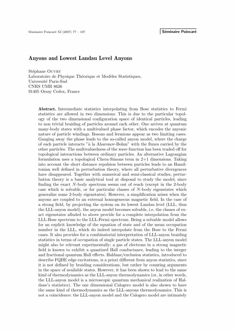
One could ask about going beyond the Fermi point α = −1 up to the Bose pointα = −2. This question is related to the validity of the LLL projection, since ignoringhigher Landau levels amounts to assuming that excited non LLL states above the N -body LLL ground state have a non vanishing gap. Considerations around the Fermipoint, as well as numerical and semiclassical analysis, support [29] this scheme aslong as α does not come close to −2. However, when α→ −2, known linear as wellas unknown nonlinear non LLL eigenstates do join the LLL ground state [31]. Saiddifferently, the LLL-anyon basis (26) does not constitute a complete LLL-Bose basiswhen α → −2, i.e. some N -body LLL bosonic quantum numbers are missing at thispoint. We will come back to this issue later.

One has not seen yet any α dependence in the N -body energy, a situationalready encountered in the 1-body A-B problem, where the free continuous energyspectrum (15) is α-independent. This is due to the fact that a magnetic field does notconfine particles: classical orbits are circular cyclotron orbits, but their centers, dueto translation invariance, are located anywhere in the plane. Translation invariance


Figure 3: Linear and non linear non LLL eigenstates merge in the LLL ground state at the bosonicvalues of α.

in turn gives, in quantum mechanics, a Landau spectrum which is li independent,and therefore infinitely degenerate2. The degeneracy factor scales as the infinitesurface V of the 2d sample: it is the flux of the magnetic field counted in units ofthe flux quantum φ0 = 2π/e (in units ~ = 1)

NL =V B

φ0(29)

Statistical interactions being topological interactions, one does not expect, in theinfinite plane limit, any effect on the N -body energies. To see such an effect, onehas to introduce a long-distance confinement, like putting the particles in a box.Let us rather introduce [30] a more convenient harmonic well confinement where theparticles are trapped, so that the Landau Hamiltonian (21) becomes

H ′N = −2

N∑

i=1

(∂i −eB

4zi)(∂i +

eB

4zi) +

1

2ω2

N∑

i=1

zizi (30)

The virtue of the harmonic confinement is to lift the degeneracy with respect tothe angular momentum li of the 1-body Landau eigenstates: the harmonic LLLspectrum3 becomes

√

ωli+1t

πli!zli

i exp(−1

2ωtzizi); li ≥ 0; E = (ωt − ωc)(li + 1) + ωc (32)

2From this point of view one can argue that the Landau spectrum is continuous, albeit being made of discreteLandau levels, due to the infinite degeneracy on each level.

3The complete 2d harmonic Landau spectrum is, with the convention eB > 0,

ωt(2ni + li + 1) − liωc; ni ≥ 0, li ∈ Z (31)

The LLL quantum numbers are ni = 0 and li ≥ 0 .


where ωt =√

ω2 + ω2c . Each harmonic LLL level in (32) has now a finite degeneracy,

with an eigenstate still analytic in zi, up to the long-distance harmonic Landaucombined exponential behavior. Let us take into account this exponential behaviorin the redefinition of the free N -body wavefunction so that (22) now becomes

ψ′(z1, z2, ..., zN ; z1, z2, ..., zN) =

∏

i<j

z−αij exp(−1

2ωt

N∑

i=1

zizi)ψ(z1, z2, ..., zN ; z1, z2, ..., zN) (33)

Starting from the Hamiltonian (30) one obtains [32, 33]

HN = −2

N∑

i=1

(∂i∂i −ωt + ωc

2zi∂i −

ωt − ωc

2zi∂i)

+ 2α∑

i<j

[ 1

zi − zj(∂i − ∂j) −

ωt − ωc

2

]

+Nωc (34)

Again let us act on N -body eigenstates made, in analogy with (25), of symmetrizedproducts of the 1-body harmonic LLL eigenstates (32)

ψ(z1, z2, ..., zN ; z1, z2, ..., zN) = Sym

N∏

i=1

zlii ; 0 ≤ l1 ≤ l2 ≤ ... ≤ lN (35)

Acting on this basis, the Hamiltonian (34) rewrites as

HN = (ωt − ωc)[

N∑

i=1

zi∂i − αN(N − 1)

2+N

]

+Nωc (36)

so that the N -anyon energy spectrum is

EN = (ωt − ωc)[

N∑

i=1

li − αN(N − 1)

2+N

]

+Nωc (37)

The N -anyon spectrum (37) is a sum of 1-body harmonic LLL spectra shifted bythe 2-body statistical term −(ωt − ωc)αN(N − 1)/2. The effect of the harmonic wellhas been not only to lift the degeneracy with respect to the li’s, but also to make theenergy dependence on α explicit. When computing thermodynamical quantities likethe equation of state, the harmonic well regulator will also be needed to computefinite quantities in a finite “harmonic” box, and then take the thermodynamic limit,by letting ω → 0 in an appropriate way.

The resulting eigenstates from (33)

ψ′(z1, z2, ..., zN ; z1, z2, ..., zN) =∏

i<j

z−αij exp(−1

2ωt

N∑

i=1

zizi)SymN∏

i=1

zlii ;

0 ≤ l1 ≤ l2 ≤ ... ≤ lN (38)


are called ”linear states” since their energy (37) varies linearly with α. As alreadystressed, they constitute a set of exact N -body eigenstates which is only a small partof the complete N -body spectrum, which remains mostly unknown. However, whatmakes, in the LLL context, these linear states particularly interesting is that theycontinuously interpolate when α = 0 → −1 from the complete harmonic LLL-Bosebasis to the complete harmonic LLL-Fermi basis.

Before turning to LLL-anyon thermodynamics, let us reconsider the physicalcharge-flux composite interpretation of the anyon model, where the charges arenow coupled to an external magnetic field. A given particle, say the Nth, sees a“positive” (eB > 0) magnetic field perpendicular to the plane, and N−1 “negative”(eφ = 2πα < 0, α ∈ [−1, 0]) point vortices piercing the plane at the positions of theother particles. This is a screening regime: in the large N limit where a mean fieldpicture is expected to be valid, the more α is close to the fermionic point α = −1, themore the external magnetic field is screened by the mean magnetic field associatedwith the vortices. In terms of the total (external + mean) magnetic field 〈B〉 thatthe Nth particle sees, or rather in terms of its flux V 〈B〉, or, when counted in unitsof the flux quantum, in terms of the Landau degeneracy 〈NL〉, one has

V 〈B〉/φ0 = (V B)/φ0 + (N − 1)φ/φ0 i.e. 〈NL〉 = NL + (N − 1)α (39)

Moving away from the Bose point, i.e. α ≤ 0, as N increases the number 〈NL〉 of1-body quantum states available for the Nth particle in the LLL of 〈B〉 decreases.This sounds reasonable, bearing in mind that a fermion occupies a quantum stateto the exclusion of others (Pauli exclusion), whereas bosons can condense (Bosecondensation). Introducing the LLL filling factor

ν =N

NL(40)

one deduces from (39) a maximal critical filling [29] for which the screening is total,〈NL〉 = 0

ν = − 1

α(41)

This is nothing but recognizing once more that bosons (α = 0) can infinitely fill aquantum state (ν = ∞), whereas fermions (α = −1) are at most one per quantumstate (ν = 1). In between, one finds that there are at most −1/α anyons per quantumstate.

Interestingly enough, Haldane/exclusion statistics definition4 happens to coin-cide with (39): for a gas of particles obeying Haldane/exclusion statistics [34] with statistical parameter g ∈ [0, 1], given NL degener-ate energy levels and N − 1 particles already populating the levels, the number dN

of quantum states still available for the Nth particle is given by (39) where −α isreplaced by g

dN = NL − (N − 1)g (42)

On the one hand, Haldane’s definition (42) stems from an arbitrary combinatorialpoint of view, inspired by the Bose and Fermi counting of states. On the other hand,in the LLL-anyon model, (39) is obtained from a somehow ad-hoc mean field ansatz.We will come back to these issues in the next section.

4This is Haldane’s statistics for one particle species. It can be generalized to the multispecies case.


3 LLL-anyon thermodynamics

Let us rewrite the N -body energy (37) as [37]

EN =N

∑

i=1

(ǫ0 + liω) − αN(N − 1)

2ω; 0 ≤ l1 ≤ l2 ≤ ... ≤ lN (43)

with ω = (ωt − ωc) and ǫ0 = ωc. Introducing the fugacity z and the inverse temper-ature β, one wants to compute the thermodynamic potential

lnZ(β, z) = ln(

∞∑

N=0

zNZN); Z0 = 1 (44)

where Z(β, z) is the grand partition function defined in terms of the N -body parti-tion functions ZN = Tr exp(−βH ′

N) = Tr exp(−βHN) = Tr exp(−βHN). The ther-modynamic potential rewrites as lnZ(β, z) =

∑∞n=1 bnz

n where, at order zn, thecluster coefficient bn only requires the knowledge of the Zi’s, with i ≤ n. One is in-terested in evaluating the thermodynamic potential in the thermodynamical limit,i.e. ω is small, which means, here, that the dimensionless quantity βω is small. TheN -body spectrum, as given in (43), allows to compute, at leading order in βω → 0,the Zi’s for i ≤ n, and thus the bn’s

bn =1

βω

e−nβωc

n2

n−1∏

k=1

k + nα

k; b1 =

1

βωe−βωc (45)

One has still to give a meaning, in the thermodynamic limit βω = 0, to the scalingfactor 1/(βω) in (45). To this purpose, one temporarily switches off the anyonicinteraction and the external magnetic field, and considers a quantum gas of noninteracting harmonic oscillators per se. One asks, when βω → 0, for its clustercoefficients to yield the infinite box (plane wave) cluster coefficients. At order n inthe cluster expansion, in d dimensions, one obtains [10]

limβω→0

(1

n(βω)2)

d2 =

V

λd(46)

where λ =√

2πβ is the thermal wavelength and V is the d-dimensional infinitevolume (in d = 2 dimensions, V is, as defined above, the infinite area of the 2dsample). Using the thermodynamic limit prescription (46), the cluster coefficient(45) rewrites, in the thermodynamic limit, as [29]

bn = NLe−nβωc

n

n−1∏

k=1

k + nα

k; b1 = NLe

−βωc (47)

The cluster expansion lnZ(β, z) =∑∞

n=1 bnzn, as a power series of ze−βωc

< 1, can be summed up

lnZ(β, z) = NL ln y(ze−βωc) (48)

where y(ze−βωc), a function of the variable ze−βωc , is such that

ln y = ze−βωc +

∞∑

n=2

(ze−βωc)n

n

n−1∏

k=1

k + nα

k(49)


It obeys [29]y − ze−βωcy1+α = 1 (50)

and has in turn a power series expansion [38]

y = 1 + ze−βωc +

∞∑

n=2

(ze−βωc)nn

∏

k=2

k + nα

k(51)

From (48) one infers that Z(β, z) = yNL so that [32, 39]

Z(β, z) = yNL = 1 +NLze−βωc +NL

∞∑

N=2

(ze−βωc)NN∏

k=2

k +NL +Nα− 1

k(52)

Clearly, from (52), the N -body partition function ZN is

ZN = NLe−Nβωc

N∏

k=2

k +NL +Nα− 1

k(53)

It is, by construction, positive. Necessarily, α and NL being given, N has to be suchthat NL +Nα ≥ 0. This always is the case as long as N is finite, since NL scales likethe infinite surface of the 2d sample. In the thermodynamic limit, where N → ∞,the condition NL +Nα ≥ 0 implies for the filling factor

ν ≤ − 1

α(54)

It is rather striking that the RHS of (54), which has just been derived from theexact computation of the cluster coefficients from the N -body spectrum, is nothingbut the critical filling (41) obtained in the mean field approach when the screeningis total.

The “degeneracy“ associated withN anyons populating the LLL quantum statesis, from (53),

NL

N∏

k=2

k +NL +Nα− 1

k=NL

N !

(N +NL +Nα− 1)!

(NL +Nα)!(55)

where a factorial with a negative argument has to be understood as (−p)! = limx→0

(−p + x)!.When α = 0, this is the usual Bose counting factor for the number of ways to

put N bosons in NL states(N +NL − 1)!

N !(NL − 1)!(56)

When α = −1, this is the Fermi counting factorNL!/(N !(NL −N)!). If one considersfor a moment the statistical parameter to be a negative integer α ≤ −1 , thedegeneracy (55) still allows for a combinatorial interpretation [38] : provided againthat NL +Nα ≥ 0, it is the number of ways to put N particles on a circle consistingofNL quantum states such that there are at least −α−1 empty states in between twooccupied states. When α = −1, this is nothing but the usual exclusion mechanismfor fermions (one fermion at most per quantum state). When α ≤ −1, i.e. beyond


the Fermi point, more and more states are excluded between two filled states. In thecase of interest α in [−1, 0], one has a ”fractional“ exclusion where one can put morethan one particle per quantum state according to the fractional α, but not infinitelymany as in the Bose case.

The degeneracy (55) originates from the exact N -body spectrum (37). In thecase of Haldane statistics as defined in (42), there is no Hamiltonian and no N -bodyspectrum to begin with. One rather starts from the Bose counting factor (56) andbluntly replaces, in accordance with (42), NL by NL − (N − 1)g to obtain

(NL − (N − 1)(g − 1))!

N !(NL − (N − 1)g − 1)!; (57)

which indeed interpolates, when g = 1, to the Fermi counting factor. The degeneracy(57) is similar to (55): if one allows the exclusion parameter g to be an integer, itcounts [38] the number of ways to put N particles on a line of finite length consistingof NL quantum states such that there are at least g − 1 empty states in betweentwo occupied states. Up to boundary conditions on the space of available quantumstates (periodic versus infinite wall), both counting (55, 57) are identical. In thethermodynamic limit when N becomes large, boundary conditions should not playa role anymore: not surprisingly, starting from (57) and following the usual route ofstatistical mechanics [40] (saddle-point approximation) leads, in the thermodynamiclimit, to the same LLL-anyon thermodynamic potential given by the equations (48)and (50), where the anyonic parameter −α is replaced by the exclusion parameterg.

Note that the grand partition factorization Z(β, z) = yNL in (48) could suggest[41] an interpretation of y as a LLL-anyon grand-partition function for a singlequantum state at energy ωc, on the same footing as, when α = 0 or α = −1,y = (1 ∓ ze−βωc)∓1 is indeed the single quantum state grand partition function fora Bose or Fermi gas. This interpretation is not possible for the reason advocatedabove: it would yield, as soon as α is fractional, negative N -body partition functions.This is clearly impossible: the N -body anyonic system is, except in the Bose andFermi cases, truly interacting and therefore its statistical mechanics is by no meansfactorisable to a single-state statistical mechanics.

From (48, 50), the average energy E ≡ −∂ lnZ(β, z)/∂β and the average parti-cle number N ≡ z∂ lnZ(β, z)/∂z or, equivalently, the filling factor ν = N/NL, canbe computed. ν satisfies

y = 1 +ν

1 + αν(58)

or, equivalently, using (50)

ze−βωc =ν

(1 + (1 + α)ν)1+α(1 + αν)−α(59)

When α 6= 0 and α 6= −1, this equation cannot in general be solved analytically,except in special cases like α = −1/2 (semions). The equation of state follows

βPV = ln(1 +ν

1 + αν) (60)

In all these equations, it is understood from (54) that ν ≤ −1/α. When ν = −1/α,the pressure diverges, a manifestation of the fact that there are as many anyons


as possible in the LLL, higher Landau levels being forbidden by construction. Onealso notes that, for the degenerate LLL gas, the filling factor in (59) is nothing butthe mean occupation number n at energy ǫ = ωc and fugacity z. As expected, (59)at α = 0 gives the standard Bose mean occupation number n = ze−βǫ/(1 − ze−βǫ),whereas at α = −1 it gives the Fermi mean occupation number n = ze−βǫ/(1+ze−βǫ).

The entropy S ≡ lnZ(β, z) + βE − (ln z)N is (trivially E = Nωc since the Nparticles are in the LLL)

S = NL

[

(1 + ν(1 + α)) ln(1 + ν(1 + α)) − (1 + να) ln(1 + να) − ν ln ν]

(61)

It vanishes when ν = −1/α, an indication that the N -body LLL anyon eigenstate isnot degenerate at the critical filling. From (37), one infers that theN -body eigenstateof lowest energy has all its one-body orbital momenta quantum numbers li = 0. Itfollows from (26) that, in the thermodynamic limit at the critical filling, the LLL-anyon non-degenerate groundstate wavefunction is

ψ′(z1, z2, ..., zN ; z1, z2, ..., zN ) =∏

i<j

z−αij exp(−1

2ωc

N∑

i=1

zizi); ν = − 1

α(62)

with total angular momentum

L =N(N − 1)

2ν(63)

The pattern in (62) is reminiscent of the Laughlin wavefunctions at FQHE fillingsν = 1/(2m+ 1)

ψ(z1, z2, ..., zN ; z1, z2, ..., zN ) =∏

i<j

z2m+1ij exp(−1

2ωc

N∑

i=1

zizi);

ν =1

2m+ 1(64)

On the one hand, Laughlin wavefunctions are fermionic, their filling factors are ratio-nal numbers smaller than 1, and they are approximate solutions to the underlyingN -body Coulomb dynamics in a strong magnetic field. On the other hand, LLL-anyon wavefunctions are multivalued, their filling factor continuously interpolatesbetween ∞ and 1, and they are exact solutions to the N -body LLL anyon problem.Still, the similarity between (62) and (64) is striking.

Trying to push (62) further beyond the Fermi point eventually up to the Bosepoint at α = −2, one obtains a Bose gas at filling ν = 1/2 with the non-degeneratewavefunction

ψ′(z1, z2, ..., zN ; z1, z2, ..., zN) =∏

i<j

z2ij exp(−1

2ωc

N∑

i=1

zizi); ν =1

2(65)

One already knows that the LLL-anyon basis (26) is not interpolating to the com-plete LLL-Bose basis when α = −2. At this point, non LLL N -body eigenstatesmerge in the LLL ground state to compensate for some missing bosonic quantumnumbers -see Figure 3. Clearly, (65) should reproduce, by periodicity, the bosonic


non-degenerate wavefunction (62) at α = 0, but it does not. On the same footing,when α = −2 the critical filling should be bosonic, i.e. ν = ∞, whereas ν = 1/2. Theunphysical critical filling discontinuity, ∞ versus 1/2, is yet another manifestationof the missing bosonic quantum numbers. In other words, the very eigenstates whichjoin the LLL ground state at the Bose point α = −2 and provide for the missingquantum numbers, have the effect to smooth out the critical filling discontinuity.Still, it has been shown [35] that the stronger the magnetic field B is, the more valid(62) remains closer and closer to α = −2. The limit α → −2 is, due to periodicity,the same as the limit α→ 0 from above, which can be described as an anti-screeningregime. One concludes that close to the Bose point α = 0, the critical filling of aLLL-anyon gas is ν = ∞ or ν = 1/2 depending on infinitesimally moving awayfrom the Bose point in the screening regime (the ground state wavefunction is theusual non degenerate bosonic wavefunction), or in the anti-screening regime (theground state wavefunction is (65)). Again, the Bose point has a somehow singularbehavior, a feature already encountered in perturbation theory. Note finally that theoccurrence of the ν = 1/2 fraction for the bosonic filling factor in the antiscreen-ing regime is physically challenging: fast rotating Bose-Einstein condensates in theFQHE regime are expected [36] to reach a 1/2 filling described by the Laughlin-likewavefunction (65).

Figure 4: The critical LLL-anyon filling curve as a function of α. The critical Bose filling ν = 1

2

occurs at the Bose points in the anti-screening regime. The continuity of the critical curve at thesepoints is restaured by the non LLL eigenstates joining the LLL ground state.

So far one has been concerned with two-dimensional systems: in the thermody-namic limit, a single particle in the LLL, and, consequently, a gas of LLL-anyons,are two dimensional, as can be seen from the NL ≃ V scalings5 of the 1-body LLLpartition function ZLLL = NL exp(−βωc) and the LLL anyon thermodynamic po-tential (48). Denoting by ρLLL(ǫ) = NLδ(ǫ − ωc) the 1-body LLL density of states,

5In the LLL there is only one quantum number li per particle, still the system is 2d.


(48) can be rewritten as

lnZ(β, z) =

∫ ∞

0

ρLLL(ǫ) ln y(ze−βǫ)dǫ (66)

Convincingly, in (66) the one-body dynamics of individual particles is described bythe one-body density of states, whereas the LLL anyon statistical collective behavioris encoded in the y function which depends on the statistical parameter α.

One might ask about other integrable N -body systems which would lead tothe same kind of statistics. It would be tempting to define a model obeying frac-tional/exclusion statistics if, its one-body density of states ρ(ǫ) being given, itsthermodynamic potential has the form

lnZ(β, z) =

∫ ∞

0

ρ(ǫ) ln y(ze−βǫ)dǫ (67)

withy − ze−βǫy1+α = 1 (68)

so that

y = 1 + ze−βǫ +∞

∑

n=2

(ze−βǫ)nn

∏

k=2

k + nα

k(69)

The mean occupation number follows as n = z∂ ln y/∂z. It obeys

y = 1 +n

1 + αn; or n =

y − 1

1 − α(y − 1)≥ 0 (70)

or, equivalently,

ze−βǫ =n

(1 + (1 + α)n)1+α(1 + αn)−α(71)

One has the duality relation [41]

1 =1

y+

1

y; where y − (ze−βǫ)−1y1+ 1

α = 1 (72)

or, equivalently

−αn− 1

αn = 1 (73)

where n is related to y as n to y in (70). The duality relation (72,73) can be in-terpreted as a particle-hole symmetry relation. Setting t = ze−βωc , one also has asimple expression [42] for dn(t)/dt

tdn

dt= n(1 + (1 + α)n)(1 + αn) (74)

All these equations have been understood as arising microscopically from theLLL anyon Hamiltonian with one-body density of states ρ(ǫ) = ρLLL(ǫ). It happensthat it is possible to find another N -body microscopic Hamiltonian which leadsto the thermodynamics (67). Consider, in one dimension, the integrable N -bodyCalogero model [43] with inverse-square 2-body interactions

HN = −1

2

N∑

i=

∂2

∂x2i

+ α(1 + α)∑

i<j

1

(xi − xj)2+

1

2ω2

N∑

i=1

x2i (75)


where xi represents the position of the i-th particle on the infinite 1d line. Thismodel is known to describe particles with nontrivial statistics in one dimensioninterpolating from Bose (α = 0) to Fermi (α = −1) statistics. It means that the1/x2 Calogero interaction is purely statistical, without any classical effect on particlemotions, up to a overall reshuffling of the particles [44]. The Calogero model remainsintegrable when, as in (75), a confining 1d harmonic well is added. This is theharmonic Calogero model, whereas the Calogero-Sutherland model [46] would havethe particles confined on a circle. The effect of the harmonic well is, as in the LLLanyon case, to lift the thermodynamic limit degeneracy in such a way that theN -body harmonic Calogero spectrum ends up depending on the Calogero couplingconstant α

EN = ω[

N∑

i=1

li − αN(N − 1)

2+N

2

]

; 0 ≤ l1 ≤ l2 ≤ ... ≤ lN (76)

Here the li’s correspond to the quantum numbers of the 1-d harmonic Hermitepolynomials free 1-body eigenstates

(ω

π)1/4 1√

2li li!e−

1

2ωx2

iHli(√ωxi); li ≥ 0; E = ω(li +

1

2) (77)

It is remarkable that (76) happens to be again of the form (43) with ω = ω,ǫ0 = ω/2. Following the same steps as in the LLL-anyon case, and using again (46)while taking the thermodynamic limit βω → 0, the Calogero cluster coefficientsrewrite as

bn =L

λ

1

n√n

n−1∏

k=1

k + nα

k; b1 =

L

λ(78)

where the infinite length of the 1d line has been denoted by L. The cluster expansioncan still be resumed using (49) provided the unwanted 1/

√n term in (78) is properly

taken care of. Introducing the 1d plane wave momentum k

1

λ√n

=1

2π

∫ ∞

−∞dke−nβ k2

2 (79)

and denoting the 1-body energy as ǫ = k2/2, one finally obtains

lnZ(β, z) =

∫ ∞

0

ρ0(ǫ) ln y(ze−βǫ)dǫ (80)

where

ρ0(ǫ) =L

π√

2ǫ(81)

is the free 1-body density of states in one dimension. This is not a surprise: in thethermodynamic limit ω → 0, where li → ∞ with liω = k2

i /2 kept fixed, the Hermitepolynomial Hli becomes a plane wave of momentum ki.

From (80), one concludes6 that, in the thermodynamic limit, the Calogero modelhas indeed a LLL-anyon/exclusion like statistics [45] according to (67) and (68),

6The same conclusion would be reached starting form the Calogero-Sutherland model and taking the correspond-ing thermodynamic limit, i.e. the radius of the confining circle going to infinity.


interpolating, as it should, from a free bosonic 1d gas at α = 0 to a free fermionic1d gas at α = −1.

It follows that the 2d LLL-anyon and 1d Calogero models, which seem a prioriunrelated, do obey the same type of statistics. This is not a coincidence. Looking attheir harmonic N -body spectrum (37) and (76), one realizes that, up to an irrelevantzero-point energy, the latter is the B → 0 limit of the former. This remains true inthe thermodynamic limit ω → 0. So, not only (66) and (80) are of the same type,but also, when B → 0, (66) has to become (80). It follows that, necessarily, the1-body densities of states ρLLL(ǫ) and ρ0(ǫ) satisfy limB→0 ρLLL(ǫ) = ρ0(ǫ), i.e.

limB→0

eBV

2πδ(ǫ− eB

2) =

L

π√

2ǫ(82)

a relation which has to be understood as arising in the thermodynamic limit ω → 0.To arrive at (82), one could as well consider directly the 1-body harmonic LLL

spectrum (32) and harmonic 1d spectrum (77)

E = (ωt − ωc)(li + 1) + ωc; E = ω(li +1

2) (83)

They are such that the latter is the vanishing B limit of the former, so it is the casefor the corresponding 1-body partition functions. Taking then7 the thermodynamiclimit βω → 0, i.e. (46), implies the relation limB→0 ZLLL = Z0, where ZLLL is,as above, the LLL partition function and Z0 is the free partition function in onedimension. Consequently for the densities of states (the inverse Laplace transforms)the relation (82) follows. This result has its roots in the different energy gaps of thespectra (83) at small ω: in the harmonic LLL case, the gap behaves like ω2/(2ωc),whereas, in the 1d harmonic case, the gap is ω.

The relation (82) could also have been understood from the 1-body eigenstatesthemselves. In the limit B → 0, the LLL induced harmonic analytic eigenstates are,from (32),

√

(ωli+1

πli!)zli

i e− 1

2ωzizi (84)

There is only one parameter ω left so that the states in (84) can be put in one-to-onecorrespondence with the Hermite polynomials (77) via the Bargmann transform

√ωli+1zli

i = ω

∫ ∞

−∞dxi

1√2lie−ω(x2

i −zixi

√2+z2

i /2)Hli(√ωxi) (85)

From (85) one can infer [47] that the N -body harmonic anyon eigenstates (38) area coherent state representation of the N -body harmonic Calogero eigenstates.

From all these considerations (thermodynamics, eigenstates,...) it follows thatthe vanishing magnetic field limit8 of the LLL-anyon model is the Calogero modelitself. It seems paradoxical to consider such a limit in the LLL which assumes a

7The order of limits is crucial here: first the limit B → 0, then the thermodynamic limit ω → 0.8Since one has ended up by taking the limit B → 0, one could have avoided right from the beginning to introduce

a B field, and started directly from the harmonic N-body anyon model. What has been done above by taking thelimit B → 0 is nothing but to project the harmonic anyon model on the LLL induced harmonic subspace (84) (theB field and its LLL should still be invoked to justify the selection of the LLL quantum numbers in the 2d harmonicbasis) and to recognize that the projected harmonic anyon model is the harmonic Calogero model. This relationremains true in the thermodynamic limit ω → 0.


priori a strong magnetic field. Still, doing so, one has dimensionally reduced the 2danyon model to the 1d Calogero model. This dimensional reduction has a simplegeometrical interpretation. The LLL induced harmonic states (84) are localized inthe vicinity of circles of radius li/ω. In the thermodynamic limit, one has li → ∞ withliω = k2

i /2 kept fixed. It follows that the corresponding 1d Hermite polynomials Hli,which become in this limit plane waves of momentum ki, have a radius of localizationdiverging like k2

i /ω2. The dimensional reduction which has taken place consists in

going at infinity on the edge of the plane: in the thermodynamic limit, the Calogeromodel can be viewed as the edge projection of the anyon model.

The LLL anyon thermodynamics, or, equivalently, the Haldane/exclusion thermodynamics, and the Calogero thermodynamics as well, have been thesubject of an intense activity since the mid-nineties. Let us mention their relevancein more abstract contexts, such as conformal field theories [48]. On the experimentalside, FQHE edge currents can be modelled by quasiparticles with fractional statis-tics, which in turn might affect their transport properties such as the current shotnoise [49, 42].

4 Minimal Difference Partitions and Trees

Up to now one has been concerned with quantum mechanical models defined bya microscopic quantum Hamiltonian. Both the LLL anyon and Calogero modelshave been shown to have a thermodynamics controlled by (67) and (68). Let usleave quantum mechanics and address a pure combinatorial problem, the minimaldifference partition problem [50]. Consider the number ρ(E,N) of partitions of aninteger E into N integer parts where each part differs from the next by at leastan integer p and the smallest part is ≥ l. Usual integer partitions correspond top = 0 and l = 1, whereas restricted partitions, where the parts have to be different,correspond to p = 1 and l = 1.

Figure 5: A minimal difference partition configuration, or Young diagram. The column heights aresuch that (li − li+1) ≥ p for i = 1, 2, . . . , N − 1 and li ≥ l. Their total height is E =

∑

N

i=1li. Wh

is the width of the Young diagram at height h, i.e. the number of columns whose heights ≥ h.


It is known that∑

E

ρ(E,N)xE =xlN+pN(N−1)/2

(1 − x)(1 − x2)...(1 − xN )(86)

The ρ(E,N) generating function Z(x, z) =∑∞

E,N ρ(E,N)xEzN factorizes when p =0 or p = 1

p = 0, Z(x, z) =

∞∏

i=0

1

1 − xl+iz; p = 1, Z(x, z) =

∞∏

i=0

(1 + xl+iz) (87)

In terms of bosons or fermions, (87) is the grand partition function for a bosonic orfermionic gas with fugacity z and, denoting x = e−β, temperature T = 1/β where

E =∞

∑

i=0

ni(l + i) N =∞

∑

i=0

ni (88)

with ni = 0, 1, 2, ... in the Bose case (p = 0) and ni = 0, 1 in the Fermi case (p = 1).Equivalently

E =

N∑

i=1

li (89)

with l ≤ l1 ≤ l2 ≤ . . . ≤ lN (Bose) or l ≤ l1 < l2 < . . . < lN (Fermi).When p is an integer ≥ 2, (86) can be regarded as the N -body partition function

of an interacting bosonic gas with the N -body spectrum

E =

N∑

i=1

li + pN(N − 1)/2; l ≤ l1 ≤ l2 ≤ . . . ≤ lN (90)

Clearly, (90) goes beyond the Fermi point p = 1 and describes some kind of ”super-fermions”. In contrast to the Bose and Fermi cases, a factorization such as (87) isnot possible, due to the interacting nature of (90). One has instead the functionalrelation

Z(x, z) = Z(x, xz) + xlzZ(x, xpz) (91)

which embodies the combinatorial identity

ρ(E,N) = ρ0

(

E − pN(N − 1)

2, N

)

(92)

where ρ0(E,N) stands for the usual partition counting.One could push [51] this analysis further to p real positive. When p ∈ [0, 1]

and l = 1, one would obtain a partition problem interpolating between the usual(bosonic) one and the restricted (fermionic) one. It is manifest that, if p is replacedby −α, the spectrum (90) coincides, under a rescaling and up to an irrelevant zero-point energy, with the N -body quantum spectrum (76) of the harmonic Calogeromodel. In a partition problem, one is interested in the large E and N asymptoticbehavior of ρ(E,N), which corresponds to the regime x → 1, i.e. β → 0. Considerthe cluster expansion lnZ(x, z) =

∑∞n=1 bnz

n. In the limit β → 0 one obtains

bn =1

β

e−nlβ

n2

n−1∏

k=1

(1 − pn

k); b1 =

1

βe−lβ (93)


The limit β → 0 should not be confused with the thermodynamic limit in quantumsystems. There is no thermodynamic limit prescription like (46). Still, using (49)(with ωc replaced by l) and taking care of the unwanted 1/n factor in (93), oneobtains, provided that ze−βl < 1,

lnZ(β, z) =

∫ ∞

l

ln y(ze−βǫ)dǫ (94)

withy − ze−βǫy1−p = 1 (95)

This is again of the form (67) and (68), the statistical parameter −α being replacedby the minimal difference partition parameter p, and the 1-body density of statesbeing the Heaviside function ρ(ǫ) = θ(ǫ−l). The minimal difference partition combi-natorics is equivalently described, in the small β limit, by a gas of particles obeyingexclusion statistics with a uniform density of states9.

This correspondence happens to be useful technically: (94) and (95) are thebuilding blocks of the minimal difference partition asymptotics. The average integerE = −∂ lnZ(β, z)/∂β =

∫ ∞lnǫdǫ and the average number of integer parts N =

z∂ lnZ(β, z)/∂z =∫ ∞

lndǫ, are both given in terms of n = z∂ ln y/∂z, the mean

occupation number at ”part” ǫ and fugacity z, which satisfies

ze−βǫ =n

(1 + (1 − p)n)1−p(1 − pn)pwith n ≤ 1

p(96)

One obtains

E − lN =1

βlnZ(β, z) N =

1

βln y(ze−βl) (97)

so that the entropy10 S ≡ lnZ(β, z) + βE − (ln z)N rewrites as

S = 2β

(

E − lN − p

2N2

)

− N ln(1 − e−βN ) (98)

with

E − lN − p

2N2 = − 1

β2

∫ 1−e−βN

0

ln(1 − u)

udu (99)

Inverting (99) gives β as a function of E and N so that the entropy S in (98) becomesa function of E and N only. Doing so, one has a definite information [51] on theasymptotic behavior of ρ(E,N) ≃ eS(E,N) when E and N are large, and also, ofρ(E) =

∑∞N=1 ρ(E,N) when E is large. One obtains a generalization of the Hardy-

Ramajunan asymptotics [52] to the minimal difference partition problem. One canalso obtain [53] the average limit shape of the Young diagrams associated with theminimal difference partition problem, generalizing the usual partition limit shape[54]. The limit shape at a part of height h depends solely on the statistical functiony evaluated at ǫ = h and at z = 1

βWh = ln y(e−βh) (100)

where β scales as β2E =∫ ∞0

ln y(e−ǫ)dǫ.

9There is no microscopic quantum Hamiltonian leading to (94) and (95).10The simple expression in (97) for N is possible because of the constant density of states.


So far p being a positive integer has insured that the N -body spectrum in (90)is well defined. However, y in (95) is still meaningful when p is a negative integer.It is the (1− p)-ary tree generating function, so that the coefficient at order n of itsexpansion in powers of ze−βǫ as given in (69) (with −α replaced by p) is the numberof ways to build a (1−p)-ary tree with n nodes. For example, at p = −1, y generatesthe Catalan numbers associated with binary trees.

Consider, as a toy model [55], the factorized (1−p)-ary tree generating function

Z(x, z) =∞∏

i=0

y(zxl+i) (101)

where y satisfies (101) with ǫ = l+ i. (101) narrows down to (87) when p = 0 (Bosecase). Its combinatorial interpretation is that ρ(E,N) deduced from (101) countsthe number of usual partitions of an integer E into N integer parts bigger or equalto l, with an additional degeneracy stemming from the (1 − p)-tree arborescencewhen, in a given partition, a part occurs n times. This enlarged degeneracy goesbeyond the Bose point to define some kind of ”superbosons”.

One can analytically continue p to the whole negative real axis. In the largeE and N limit, i.e. β smaller and smaller, one encounters a maximal temperaturebeyond which it is not possible to heat the system. Indeed, from (95) it follows thaty(zxl+i) in (101) obeys to y − ze−β(l+i)y1−p = 1, which is well defined only if [39]

ze−βl < (1 − p)p−1(−p)−p < 1 (102)

When z = 1, it defines a dimensionless ”Hagedorn temperature”

T =l

(1 − p) ln(1 − p) + p ln(−p) (103)

just below which E and N become large so that the asymptotic of ρ(E,N) can beaddressed.

5 Conclusion

In two dimensions intermediate anyonic statistics interpolating from Bose to Fermistatistics are allowed. Their definition does not involve anything else than the usualconcept at the basis of quantum statistics, namely free particles endowed with par-ticular boundary exchange conditions on their N -body wavefunctions. It happensthat these boundary conditions have a much richer structure in two dimensionsthan in three and higher dimensions. This in turn can be understood in terms of thetopology of paths in the N -particle configuration space, where non trivial braidingoccurs in two dimensions, and not in higher dimensions. A flux-charge compositepicture emerges to encode the braiding statistics in physical terms, via topologicalAharonov-Bohm interactions and singular magnetic fields.

The anyon model as such is certainly fascinating as far as quantum mechanicsis concerned, but it remains an abstract construction whose complexity is daunting.However, when projected onto the LLL of an external magnetic field, the modelbecomes tractable and, even more, solvable. The LLL set up is clearly adaptedto the QHE and to the FQHE physics. Haldane/exclusion statistics, which can be


obtained as a LLL-anyon mean-field picture in the screening regime, leads to LLL-anyon thermodynamics.

It would certainly be rewarding if LLL anyons could be relevant experimentally,for example by uncovering some experimental hints at FQHE filling factors of the ex-istence of quasiparticles with anyonic/exclusion statistics. Fractional charges have already been seen in shot noise FQHEexperiments [56], but the nontrivial statistical nature of the charge carriers in FQHEedge currents has so far remained elusive in experiments which rely mainly onAharonov-Bohm interferometry [28]. Note also a recent proposal for the possibleexperimental tracking of abelian and nonabelian anyonic statistics in Mach-Zehnderinterferometers [57].

Finally, on the theoretical side, physical interactions, together with topologicalanyonic interactions, should also be taken into account in order to produce morerealistic models.

Acknowledgments

I would like to thank Alain Comtet and Stefan Mashkevich for past and presentcollaborations, and for correcting and improving the text. My thanks also to TobiasPaul and Sanjib Sabhapandit for helping me with the Figures.

References

[1] J.M. Leinaas, J. Myrheim, On the theory of identical particles, Nuovo Cimento37B (1977), 1–23. For an earlier work on the subject see: M.G.G. Laidlaw,C.M. de Witt, Feynman Functional Integrals for Systems of IndistinguishableParticles, Phys. Rev D3 (1971), 1375.

[2] For a recent review on spin issues related to statistics see: S. Forte, Spin in quan-tum field theory, Proceedings of the 43th Internationale Univeritastswochen furTheoretiche Physik, Schladming, Austria (2005). arXiv: hep-th/0507291

[3] G. Moore, N. Seiberg, Polynomial equations for rational conformal field theories,Phys. Lett. B 212 (1988), 451. Classical and quantum conformal field theory,Commun. Math. Phys. 123 (1989), 177. G. Moore, N. Read, Nonabelions in thefractional quantum Hall effect, Nucl. Phys. B 360 (2-3) (1991), 362.

[4] A.Yu. Kitaev, Fault-tolerant quantum computation by anyons, Ann. Phys. 303

(2003), 2–30.

[5] F. Wilczek, Magnetic flux, angular momentum, and statistics, Phys. Rev. Lett.48 (1982), 1144–1146. Quantum mechanics of fractional-spin particles,Phys. Rev. Lett. 49 (1982), 957–959.

[6] Y. Aharonov, D. Bohm, Significance of electromagnetic potentials in quantumtheory, Phys. Rev. 115 (1959), 485–491. For an earlier work on the subjectsee: W. Ehrenberg, R.W. Siday, The Refractive index in electron optics and theprinciples of dynamics, Proc. Phys. Soc. London B62 (1949), 8–21.

[7] R.G. Chambers, Shift of an electron interference pattern by enclosed magneticFlux, Phys. Rev. Lett. 5 (1960), 3.


[8] Tsuyoshi Matsuda, Shuji Hasegawa, Masukazu Igarashi, Toshio Kobayashi,Masayoshi Naito, Hiroshi Kajiyama, Junji Endo, Nobuyuki Osakabe, AkiraTonomura, Ryozo Aoki, Magnetic field observation of a single flux quantumby electron-holographic interferometry, Phys. Rev. Lett. 62 (1989), 2519.

[9] W. Siegel, Unextended superfields in extended supersymmetry, Nucl. Phys. B156

(1979), 135–143. J.F. Schonfeld, A mass term for three-dimensional gaugefields, Nucl. Phys. B185 (1981), 157–171. R. Jackiw, S. Templeton, How super-renormalizable interactions cure their infrared divergences, Phys. Rev. D 23(1981), 2291–2304. S. Deser, R. Jackiw, S. Templeton, Three-dimensional mas-sive gauge theories, Phys. Rev. Lett. 48 (1982), 975–978. Topologically massivegauge theories, Ann. Phys. (N.Y.) 140 (1982), 372–411.

[10] J. McCabe, S. Ouvry, Perturbative three-body spectrum and the third virial co-efficient in the anyon model, Phys. Lett. B 260 (1991), 113–119.

[11] S. Ouvry, δ perturbative interactions in the Aharonov-Bohm and anyon mod-els, Phys. Rev. D 50 (1994), 5296–5299. A. Comtet, S.V. Mashkevich, S. Ou-vry, Magnetic moment and perturbation theory with singular magnetic fields,Phys. Rev. D 52 (1995), 2594–2597.

[12] C. Manuel, R. Tarrach, Contact interactions of anyons, Phys. Lett. B 268(1991), 222–226.

[13] For a review on the anyon model, see (among others): J. Myrheim, Anyons, LesHouches LXIX Summer School ”Topological aspects of low dimensional systems”(1998) 265–414.

[14] Y.-S. Wu, Multiparticle quantum mechanics obeying fractional statistics,Phys. Rev. Lett. 53 (1984), 111–114.

[15] A.P. Polychronakos, Exact anyonic states for a general quadratic hamiltonian,Phys. Lett. B 264 (1991), 362–366. C. Chou, Multianyon spectra and wavefunctions, Phys. Rev. D 44 (1991), 2533–2547. S.V. Mashkevich, Exact solu-tions of the many-anyon problem, Int. J. Mod. Phys. A 7 (1992), 7931–7942.G. Dunne, A. Lerda, S. Sciuto, C.A. Trugenberger, Exact multi-anyon wavefunctions in a magnetic field, Nucl. Phys. B 370 (1992), 601–635. A. Karlhede,E. Westerberg, Anyons in a magnetic field, Int. J. Mod. Phys. B 6 (1992), 1595–1621. S.V. Mashkevich, Towards the exact spectrum of the three-anyon problem,Phys. Lett. B 295 (1992), 233–236.

[16] D. Arovas, R. Schrieffer, F. Wilczek, A. Zee, Statistical mechanics of anyons,Nucl. Phys. B 251 (1985), 117–126.

[17] A. Comtet, Y. Georgelin, S. Ouvry, Statistical aspects of the anyon model, J.Phys. A: Math. Gen. 22 (1989), 3917–3926.

[18] D. Sen, Spectrum of three anyons in a harmonic potential and the third virialcoefficient, Phys. Rev. Lett. 68 (1992), 2977–2980. M. Sporre, J.J.M. Ver-baarschot, I. Zahed, Anyon spectra and the third virial coefficient, Nucl. Phys.B 389 (1993), 645–665.


[19] M. Sporre, J.J.M. Verbaarschot, I. Zahed, Numerical solution of the three-anyon problem, Phys. Rev. Lett. 67 (1991), 1813–1816. M.V.N. Murthy, J. Law,M. Brack, R.K. Bhaduri, Quantum spectrum of three anyons in an oscillator po-tential, Phys. Rev. Lett. 67 (1991), 1817–1820. M. Sporre, J.J.M. Verbaarschot,I. Zahed, Four anyons in a harmonic well, Phys. Rev. B 46 (1992), 5738–5741.

[20] R.K. Bhaduri, R.S. Bhalerao, A. Khare, J. Law, M.V.N. Murthy, Semiclassicaltwo- and three-anyon partition functions, Phys. Rev. Lett. 66 (1991), 523–526.F. Illuminati, F. Ravndal, J.Aa. Ruud, A semi-classical approximation to thethree-anyon spectrum, Phys. Lett. A 161 (1992), 323–325. J.Aa. Ruud, F. Ravn-dal, Systematics of the N-anyon spectrum, Phys. Lett. B 291 (1992), 137–141.

[21] A. Comtet, J. McCabe, S. Ouvry, Perturbative equation of state for a gas ofanyons, Phys. Lett. B260 (1991) 372–376.

[22] A. Dasnieres de Veigy, S. Ouvry, Perturbative equation of state for a gas ofanyons: Second order, Phys. Lett. B 291 (1992), 130–136. Perturbative anyongas, Nucl. Phys. B 388 (1992), 715–755.

[23] J. Myrheim, K. Olaussen, The third virial coefficient of free anyons, Phys.Lett. B 299 (1993), 267–272. S.V. Mashkevich, J. Myrheim, K. Olaussen, Thethird virial coefficient of anyons revisited, Phys. Lett. B 382 (1996), 124–130.A. Kristoffersen, S.V. Mashkevich, J. Myrheim, K. Olaussen, The fourth virialcoefficient of anyons, Int. J. Mod. Phys. A 11 (1998), 3723–3747. S.V. Mashke-vich, J. Myrheim, K. Olaussen, R. Rietman, The nature of the three-anyon wavefunctions, Phys. Lett. B 348 (1995), 473–480.

[24] R.B. Laughlin, Quantized Hall conductivity in two dimensions, Phys. Rev. B 23(1981), 5632–5633. Anomalous quantum Hall effect: An incompressible quantumfluid with fractionally charged excitations, Phys. Rev. Lett. 50 (1983), 1395–1398. Quantized motion of three two-dimensional electrons in a strong magneticfield, Phys. Rev. B 27 (1983), 3383–3389. See also: F.D.M. Haldane, Fractionalquantization of the Hall effect: A hierarchy of incompressible quantum fluidStates, Phys. Rev. Lett. 51 (1983), 605–608.

[25] K. von Klitzing, G. Dorda, M. Pepper, New method for high-accuracy de-termination of the fine-structure constant based on quantized Hall resistance,Phys. Rev. Lett. 45 (1980), 494–497. D.C. Tsui, H.L. Stormer, A.C. Gossard,Zero-resistance state of two-dimensional electrons in a quantizing magnetic field,Phys. Rev. B 25 (1982), 1405–1407. M.A. Paalanen, D.C. Tsui, A.C. Gossard,Quantized Hall effect at low temperatures, Phys. Rev. B 25 (1982), 5566–5569.H.L. Stormer, A. Chang, D.C. Tsui, J.C.M. Hwang, A.C. Gossard, W. Wieg-mann, Fractional quantization of the Hall effect, Phys. Rev. Lett. 50 (1983),1953–1956.

[26] D.P. Arovas, R. Schrieffer, F. Wilczek, Fractional statistics and the quan-tum Hall effect, Phys. Rev. Lett. 53 (1994), 722–725. B.I. Halperin, Statis-tics of quasiparticles and the hierarchy of fractional quantized Hall states,Phys. Rev. Lett. 52 (1984), 1583–1586.

[27] H. Kjønsberg, J. Myrheim, Numerical study of charge and statistics of Laughlinquasiparticles, Int. J. Mod. Phys. A 14 (1999), 537–557. D. Banerjee, Topological


aspects of phases in fractional quantum Hall effect, Phys. Lett. A 269 (2000),138–143.

[28] F.E. Camino, W. Zhou, V.J. Goldman, Aharonov-Bohm electron interferometerin the integer quantum Hall regime, arXiv: cond-mat/0503456. Experimental re-alization of Laughlin quasiparticle interferometers, Proc. of EP2DS-17 (Genoa,Italy, 2007). arXiv:0710.1633.

[29] A. Dasnieres de Veigy, S. Ouvry, Equation of state of an anyon gas in a strongmagnetic field, Phys. Rev. Lett. 72 (1994), 600–603.

[30] E. Fermi was the first to introduce an harmonic well confinement to com-pute thermodynamical quantities: E. Fermi, Sulla quantizzazione del gas per-fetto monoatomico, Rend. Lincei 3 (1926), 145. In the anyon context, the har-monic well confinement was first used in [17]. See also: K. Olaussen, On theharmonic oscillator regularization of partition functions, Trondheim preprintNo. 13 (1992).

[31] S.V. Mashkevich, J. Myrheim, K. Olaussen, R. Rietman, Anyon trajectories andthe systematics of the three-anyon spectrum, Int. J. Mod. Phys. A 11 (1996),1299–1313.

[32] S. Ouvry, On the relation between the anyon and the Calogero Models, Phys.Lett. B 510 (2001), 335.

[33] S. Isakov, G. Lozano, S. Ouvry, Non abelian Chern-Simons particles in an ex-ternal magnetic field, Nucl. Phys. B 552 [FS] (1999), 677.

[34] F.D.M. Haldane, “Fractional statistics” in arbitrary dimensions: A generaliza-tion of the Pauli principle, Phys. Rev. Lett. 67 (1991), 937–940.

[35] S.V. Mashkevich, S. Ouvry, The lowest Landau level anyon equation of state inthe anti-screening regime, Phys. Lett. A 310 (2003), 85–94.

[36] N.K. Wilkin, J.M. Gunn, R.A. Smith,Do attractive bosons condense?, Phys.Rev. Lett. 80 (1998), 2265.

[37] A. Dasnieres de Veigy, S. Ouvry, One-dimensional statistical mechanics for iden-tical particles : the Calogero and anyon cases, Mod. Phys. Lett. B 9 (1995), 271.

[38] A.P. Polychronakos, Probabilities and path-integral realization of exclusionstatistics. arXiv: hep-th/9503077. See also: Generalized statistics in one dimen-sion, Les Houches LXIX Summer School ”Topological aspects of low dimensionalsystems” (1998) 415–472.

[39] A.G. Bytsko, Haldane-Wu statistics and Rogers dilogarithm, Zap. Nauchn.Semin. POMI 291 (2002), 64–77, J. Math. Sciences 125 (2005), 136–143.

[40] Y.S. Wu, Statistical distribution for generalized ideal gas of fractional-statisticsparticles, Phys. Rev. Lett. 73 (1994), 922–925.

[41] C. Nayak, F. Wilczek, Exclusion statistics: Low-temperature properties, fluctua-tions, duality, and applications, Phys. Rev. Lett. 73 (1994), 2740. S. Chaturvedi,V. Srinivasan, Microscopic interpretation of Haldane’s semion statistics, Phys.Rev. Lett. 78 (1997), 4316. M.V.N. Murthy, R. Shankar, Exclusion statistics: Aresolution of the problem of negative weights, Phys. Rev. B 60 (1999), 6517.


[42] G. Gomila, L. Reggiani, Fractional exclusion statistics and shot noise in ballisticconductors, Phys. Rev. B 63 (2001), 165404.

[43] F. Calogero, Solution of a three-body problem in one dimension, J. Math. Phys.10 (1969), 2191–2196. Ground state of a one-dimensional N-body system, J.Math. Phys. 10 (1969), 2197–2200. Solution of the one-dimensional N-bodyproblems with quadratic and/or inversely quadratic pair potentials, J. Math.Phys. 12 (1971), 419–436.

[44] For a recent review on the Calogero model, see (among others): A.P. Polychron-akos, Physics and mathematics of Calogero particles. arXiv: hep-th/0607033.

[45] A.P. Polychronakos, Non-relativistic bosonization and fractional statistics, Nucl.Phys. B324 (1989), 597. Exchange operator formalism for integrable systems ofparticles, Phys. Rev. Lett. 69 (1992), 703. S. B. Isakov, Fractional statistics inone dimension: Modeling by means of 1/x2 interaction and statistical mechanics,Int. J. Mod. Phys. A 9 (1994), 2563. Generalization of statistics for severalspecies of identical particles, Mod. Phys. Lett. B 8 (1994), 319. Bosonic andfermionic single-particle states in the Haldane approach to statistics for identicalparticles, Phys. Rev. B 53 (1996), 6585–6590. D. Bernard, Y.-S. Wu, A Noteon statistical interactions and the thermodynamic Bethe ansatz, (1994). arXiv:cond-mat/9404025. [

[46] B. Sutherland, Quantum many-body problem in one dimension: Ground state,J. Math. Phys. 12 (1971), 246–250. Quantum many-body problem in one dimen-sion: Thermodynamics, J. Math. Phys. 12 (1971), 251–256.

[47] L. Brink, T.H. Hansson, S. Konstein, M.A. Vasiliev, The Calogero model anyonicrepresentation, fermionic extension and supersymmetry, Nucl. Phys. B 401,Issue 3 (1993), 591–612.

[48] K. Schoutens, Exclusion statistics in conformal field theory spectra,Phys. Rev. Lett. 79 (1997), 2608–2611. P. Fendley, K. Schoutens, Cooper pairsand exclusion statistics from coupled free-fermion chains, J. Stat. Mech. 0207

(2007), 17.

[49] S. Isakov, T. Martin, S. Ouvry, Conductance and shot noise for particles withexclusion statistics, Phys. Rev. Lett. 83 (1999), 580.

[50] G.E. Andrews, The Theory of partitions, Cambridge University Press, Cam-bridge (1998). G.E. Andrews, R. Askey, R. Roy, Special functions, Encyclopediaof Mathematics and its applications 71, Cambridge University Press, Cambridge(1999).

[51] A. Comtet, S.N. Majumdar, S. Ouvry, Integer partitions and exclusion statistics,J. Phys. A: Math. Theor. 40 (2007), 11255.

[52] G.H. Hardy, S. Ramanujan, Proc. London. Math. Soc. 17 (1918), 75.

[53] A. Comtet, S.N. Majumdar, S. Ouvry, S. Sabhapandit, Integer partitions andexclusion statistics: Limit shapes and the largest part of Young diagrams, J.Stat. Mech. (2007) P10001.


[54] A.M. Vershik, Statistical mechanics of combinatorial partitions and their limitshapes, Functional Analysis and Its Applications 30 (1996), 90.

[55] A. Comtet, S.N. Majumdar, S. Ouvry, S. Sabhapandit, in preparation.

[56] L. Saminadayar, D.C. Glattli, Y. Jin, B. Etienne, Observation of the e/3 frac-tionally charged Laughlin quasiparticle, Phys. Rev. Lett 79 (1997), 162. R. de-Picciotto et al, Nature 389 (1997), 162.

[57] D. E. Feldman, Y. Gefen, A.Yu. Kitaev, K. T. Law, A. Stern, Shot noise inanyonic Mach-Zehnder interferometer, Phys. Rev. B 76 (2007), 085333.

Anyons and Lowest Landau Level Anyons - · PDF file · 2007-12-21Anyons and Lowest...

Documents

Transcript of Anyons and Lowest Landau Level Anyons - · PDF file · 2007-12-21Anyons and Lowest...