Brigham Young UniversityBYU ScholarsArchive

All Theses and Dissertations

1964-05-30

An Experimental Investigation of the Effect of aConstant Body Force Field Upon the DragCoefficient of a SphereBrent Evans BoyackBrigham Young University - Provo

Follow this and additional works at: https://scholarsarchive.byu.edu/etd

Part of the Mechanical Engineering Commons

This Thesis is brought to you for free and open access by BYU ScholarsArchive. It has been accepted for inclusion in All Theses and Dissertations by anauthorized administrator of BYU ScholarsArchive. For more information, please contact scholarsarchive@byu.edu, ellen_amatangelo@byu.edu.

BYU ScholarsArchive CitationBoyack, Brent Evans, "An Experimental Investigation of the Effect of a Constant Body Force Field Upon the Drag Coefficient of aSphere" (1964). All Theses and Dissertations. 7077.https://scholarsarchive.byu.edu/etd/7077

AN EXPERIMENTAL INVESTIGATION OF THE EFFECT OF A CONSTANT BODY FORCE FIELD UPON

THE DRAG COEFFICIENT OF A SPHERE

A Thesis Presented to the

Department of Mechanical Engineering Science

BRIGHAM YOUNG UNIVERSITY

in partial fulfillment of the requirements for the degree

of

Master of Science in

Mechanical Engineering

by

Brant Evans Boyack

April 1964

DEDICATION

To my wife, Marcia, and my son, Kevin.

ACKNOWLEDGMENT

The author wishes to express his appreciation to Dr. John M.

Simonsen for his counsel and assistance.

iii

APPROVALS

This

requirement Department,

thesis is accepted in its present form as fulfilling the thesis

toward a Master of Science degree in the Mechanical Engineering Brigham Young University.

_52Date

LZ. ) {t*Date

Date

3ô iLDate /

iv

TABLE OF CONTENTSPage

ACKNOWLEDGMENT........................................................ iii

APPROVALS.......................................................... ivTABLE OF CONTENTS.................................................. v

LIST OF F I G U R E S ...................................................... vilNOMENCLATURE ...................................................... . viiiChapter

I. INTRODUCTION ................................................ 1

Dimensionless Relationships . . . ........................ 2S c o p e .................................................... 8

II. LITERATURE SURVEY .......................................... 9

III. TEST APPARATUS.............................................. 21

Test Chamber.............................................. 22Particle Drop Mechanism.................................. 22Sequence Control .......................................... 24Timing Equipment ........................................... 24

IV. DATA ACQUISITION AND REDUCTION TECHNIQUE................... 26

Data Acquisition.......................................... 27Data Reduction............................................ 28Raw Data Determination.................................. 28Computer Reduction of D a t a ........... 30

V. R E S U L T S .................................................... 32

Discussion of Results .................................... 33Reproducibility.......................... 36Boundary Condition........................ 36Comparison.............................................. 37

Computer Program.......................................... 37Significance.................................. 38

VI. CONCLUSIONS............................................... 40

v

Page

LIST OF REFERENCES.................................................. 42APPENDIX A - ERROR ANALYSIS........................................ 45

APPENDIX B - DATA REDUCTION P R O G R A M ................................ 49APPENDIX C - EQUATION DERIVATION .................................... 55

ABSTRACT OF THESIS.................................................. 57

vi

LIST OF FIGURES

Figure Page

1. The Steady State Drag Curve for S p h e r e s ...................... 5

2. Comparative Ranges of Acceleration Drag D a t a .................. II3. Drag Coefficients for Accelerating Spheres .................... 134. The Drag Coefficients of Spheres as a Function of Acceleration

and Reynolds N u m b e r .......................................... 15

5. The Drag Coefficients of Cylinders Accelerating from Rest . . . 166. Drag Coefficients for Spray Particles Accelerated in Moving Air

Streams . .............. 18

7. Drag Coefficients as a Function of Reynolds Number............. 198. Vacuum Particle Drop Schematic........... 239. Electronic Timing Equipment Schematic ........................ 25

10. Typical Data Photograph...................................... 2911. Measured Drag Coefficients as a Function of Reynolds Number . . 3412. Curves of Constant Acceleration Modulus ...................... 35

vii

NOMENCLATURE

A Projected body area

cd Drag coefficient

Cmd Distance from camera lens to sphere

Ds Sphere diameter

Fb Buoyant force

Fd Drag force

F8 Gravitational force

j Time rate of change of acceleration

LP Characteristic lengthM Sphere mass

«a Acceleration modulus

N j Jerk modulus

Nr Reynolds number

vn The nth variable

Vs-f Velocity of sphere relative to the fluid

▼s-£ Acceleration of sphere relative to the fluid

VP Particle velocity

Y P Particle acceleration

vt Terminal velocity

Wn Error in measurement of Vn

Ya Actual sphere displacement

Yi Measured sphere displacement

Ymp Distance from reference point to center of photograph

viii

P"Sphere density

pi Fluid density

J4 f Dynamic fluid viscosity

tf Specific gravity of the fluidSnX/Stn nth partial derivative of position with respect to time

ix

CHAPTER IINTRODUCTION

INTRODUCTION

The object of this thesis was to present the method and results of an experimental determination and correlation of the drag coefficients of

accelerating spheres.This investigation was the result of a need for basic information

and understanding of solids-gas systems. There are many areas in which information about particle drag coefficients is applicable providing the data is known to be reliable. One of the most important of these is the analysis of a particle laden gas flow through either a rocket nozzle or a

flow confining passageway. In fact, reliable data could be applied to the analysis and design of any object which moves about in either a gas or liquid medium with acceleration.

To this time, there has been a need for basic research into the effect which acceleration has on particle drag and hence particle drag coefficients. The various sources of data which are available at the time

of writing do not agree, and in fact, offer little basis for comparison with each other. It was evident that there was a need for investigation of possible parameters which may be of importance in understanding and

correlating various sources of data.

Dimensionless Relationships

The drag force acting upon a body which is moving through a fluid is equal to the surface integral of all the normal and shearing stresses act­ing upon the body. The process of dimensional analysis is used to derive

2

3

a dimensionless parameter which is associated with this force. The parame­ter is called the coefficient of drag and is defined as:

Cd = ---— — —\?t Vl_f A

Where

Cd is the drag coefficient

Fd is the drag force

A is the projection of the body area onto a plane normal to the path of the body

Vg_£ is the velocity of the sphere relative to the fluid

Pt is the density of the fluid

The drag coefficient is related to other dimensionless parameters. One of these is the Reynolds number. It physically represents the ratio of the inertial to the viscous forces. The Reynolds number is defined as:

Nr Pi Vs-f os

Where

Nr is the Reynolds number

Dg is the sphere diameter (characteristic length) is the dynamic viscosity of the fluid

To aid in the understanding of the effect which acceleration has onthe drag coefficient, another dimensionless parameter is used. This

4

parameter is called the acceleration modulus and is defined as:

©Where

Nfi is the acceleration modulusVg_£ is the relative acceleration between the sphere

and the fluid

The acceleration modulus was derived by Keim<'~^* and has previouslybeen used to correlate drag data of accelerating circular disks and cylinders.

Acceleration effects may also be correlated by using the jerk modulus. The jerk modulus is defined as:

Steady State Drag

Extensive experimentation has been performed in the study of steady

state drag. The commonly accepted drag curve is shown in Figure 1. This

curve applies to the motion of a single sphere at a constant velocity through an infinite, continuous, incompressible, turbulence free fluid. Although these idealized conditions are seldom the case in actual flow, a

Numbers in parenthesis refer to References.

Where

Nj is the jerk modulusj is the time rate of change of acceleration

DRAG

COEFFICIENT

REYNOLDS NUMBER, Nr

Figure 1. The steady state drag curve for spheres. (Reference 2)

Ln

6knowledge of the fundamental concepts underlying the ideal motion is es­

sential for the proper understanding and evaluation of the complicating effects encountered in accelerating flow.

There are six important and definable Reynolds number regimes associated with the steady state drag curve. Significant flow patterns around a sphere occur in each regime. The regimes will be discussed in the following paragraphs.

For small Reynolds numbers, Nr <l, the flow is everywhere non- turbulent and the drag is referred to as the deformation drag. The flow in this region is known as Stokes flow, and an analytical expression describing the flow can be derived from the Navier-Stokes equations by neglecting the momentum terms. Viscous forces predominate in this regime and the flow is attached.

A separation process in the boundary layer first begins at aIReynolds number of approximately one. The streamline patterns associated

with the Stokes regime become deformed and curl up to form a stationary vortex ring in the boundary layer at the rear of the sphere. This ring, resembling a smoke ring with axial symmetry, grows in size as the Reynolds

number is increased. The vorticity generated in the ring is balanced by that which diffuses downstream from the ring. Flow around the sphere is retarded by an adverse pressure gradient which increases with increasing

Reynolds number. Separation occurs at the surface of the sphere when the

energy and momentum of the fluid in the boundary layer are insufficient to overcome the adverse pressure gradient.

At a Reynolds number of about 500, for a stream free from turbulence, a point of imbalance is reached where the vorticity diffusion rate down­stream can no longer keep up with that generated in the vortex ring. At

7this point, the vortex system breaks away from the body and feeds into a flow region behind the sphere which is bounded by the separated bound­ary layer. This flow region is referred to as the wake. A new ring forms as the unstable one detaches so that there is a periodicity asso­ciated with the wake flow in this Reynolds number regime. As the Reynolds

number increases past 500 there is a laminar-turbulent transition in the wake which creeps toward the separation point. The gradual increase in

drag coefficient for Nr> 5X10^ may be caused by this shifting toward the sphere of the laminar-turbulent transition point in the separated boundary layer.

For the Reynolds number regime defined by 2X10^< N r< 3X10^, the wake is made up of random eddys in which the proportion of turbulent

fluctuations predominate as the Reynolds number increases.The sharp decrease in the drag coefficient near Nr = 3X10^ rep­

resents a transition in the boundary layer from laminar to turbulent flow. The turbulent boundary layer absorbs energy from the free stream

and enables the flow to proceed further around the sphere before it sepa­rates. Specifically, the boundary layer separation ring moves from in front of the equator to in back of the equator, thereby reducing the size of the wake behind the sphere. The pressure distribution becomes more like that for a frictionless motion, and the pressure drag is decreased.

For Reynolds numbers greater than 3X10^, the boundary layer flow

is turbulent. The wake is relatively narrow, turbulent, and statistically stable. The drag coefficient increases monotonically with increasing Reynolds number.

The resistance of a sphere to motion in a fluid is the sum of the skin friction drag and a pressure or form drag. Pressure drag is intimately

associated with the mechanism of flow in the wake region. The relative contribution from each type of resistance varies with the flow regime.

Skin friction drag accounts for two-thirds of the total drag in the Stokes Law regime, but its contribution when compared with that of the pressure drag steadily diminishes to a negligible value as the Reynolds

number is increased beyond this range.

Scope

There are a number of factors which influence the drag force acting upon a sphere as it moves through a fluid. The most important of these factors are listed belowî

Reynolds number^) Acceleration^) Turbulence^) Rotation^)Knudsen number^)

Mach number^)Wall effects Heat transfer^) Surface roughness^®)

Due to the small number of applicable investigations, there is a limited amount of information dealing with the effect of each of these factors upon particle drag coefficients. A comprehensive review of the

available information is given by Scott^*-) and is useful in determining the relative importance of each factor in a particular flow situation.

The scope of this thesis consisted of examining the results of selected investigations which describe the non-steady drag coefficients of accelerating bodies, developing reliable equipment and methods of obtain­ing reproducible displacement-time data, and comparing the drag coefficients obtained in this investigation with those obtained from Lunnon's^^) data.

8

CHAPTER XILITERATURE SURVEY

LITERATURE SURVEY

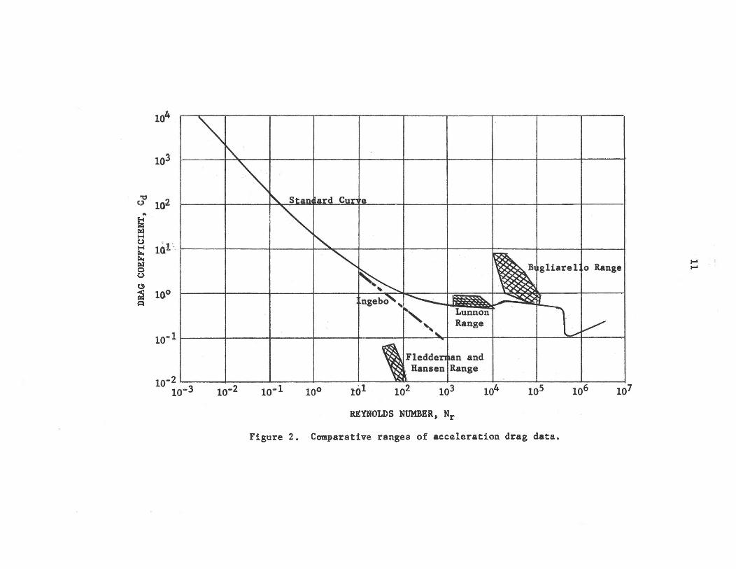
The documentation of efforts to determine the effect of accelerationlupon particle drag coefficients is limited in both scope and volume. Figure 2 summarizes the relative regimes of the data which will be discussed in this survey. It indicates the inconclusiveness of the data so far obtained and the need for many energetic inquiries which will provide reliable, quanti­

tative drag values as well as further insight into the fluid dynamics of unsteady motion.

Investigations of the acceleration effect have been divided into three general categories, depending upon whether the bodies move relative to the fluid--(1) in constant, rectilinear acceleration; (2) in variable,

rectilinear acceleration; and (3) with an oscillatory motion. The experi­

mental part of this thesis is concerned with variable, rectilinear acceler­ation, but the other two types of acceleration will be discussed for the

insight they offer into the total problem of the effect of acceleration upon particle drag coefficients.

In 1826, Bessel^^) reported experiments with a spheroid pendulum

moving in air and in water. He found that the movement of the pendulum

could not be accounted for by the conventional equations of motion and so introduced an "added mass," which was proportional to the mass of the fluid displaced by the body. The added mass concept has since been shown to be completely inadequate and theoretically unsound as it does not describe the complex flow associated with accelerated motion.

10

DRAG

COEFFICIENT

REYNOLDS NUMBER, Nr

Figure 2. Comparative ranges of acceleration drag data.

H*h-»

12One of the earliest studies of rectilinear motion which hinted at

possible acceleration effects was reported in 1900 by Allen^*"^. He noted that the drag coefficients of spheres slowly accelerating in water were increased from ten to twenty per cent over steady state values. Increased values of the drag coefficient resulting from the acceleration of spheres in water were also reported by Magnan and St. Lague^^^ and Cook^^ .

The variable, rectilinear acceleration of an object has been studied in several investigations. Bugliarelle^^) published a series of results

obtained with spheres which were drawn by constant forces up through a stag­nant pool of water. The added mass concept was found to be completely in­

applicable. The plots of the drag coefficient versus Reynolds number are considerably scattered. They show drag coefficients with values as high as

30, compared to the steady state value of 0.4. Bugliarello's data is shown in Figure 3. It should be noted that the data is questioned since the wire towed sphere had an apparent shape other than that of a true sphere. The flow pattern around a string or wire pulled sphere is not the same as the

flow pattern around a sphere which does not have any apparatus attached to it. In some cases the wire attached to a sphere causes separation even at

the stagnation point.Luneau^?) and Johnson and Laird(^8) have studied the effects of a

constant acceleration upon the particle drag coefficients of circular disks

and cylinders respectively, but insufficient data were presented to draw any

usable conclusions.Lunnoa^^) studied the motion of spheres falling with a variable,

rectilinear acceleration in both air and water and was able to obtain

highly reproducible results. This investigation is noted for its excellent technique. The displacement-time data for spheres falling in air was

DRAG

COEFFICIENT

13

Figure 3. Drag coefficients for accelerating spheres. (Bugliarello, References 16 and 3)

14reduced to obtain the particle accelerations as shown in Figure 4. It can be seen that even moderate accelerations can have marked effects on

the drag coefficient, depending upon the particle Reynolds number regime.Iverson and B a i e n t studied the acceleration of circular disks

towed by a fine weighted cable. From an examination of the Navier-Stokes

equations, it was felt the drag coefficient should be a function of (LpVpp^M), (Vp/gL) and (VpLp/V^) where Lp is a characteristic length, Vp

is the body velocity and Vp is the body acceleration. The last group, the acceleration modulus, was found to correlate all the coefficient of drag values on one smooth curve showing no dependency upon the Reynolds number. It was also shown that the added mass concept failed to explain

the large dependence of the fluid resistance on the particle acceleration.Keirn^1) measured the drag coefficients of both circular disks and

cylinders. His work with circular disks agrees favorably with that of Iverson and Baient. The drag coefficients for cylinders of various length- to-diaraeter ratios showed an explicit dependency upon the Reynolds number, (VpD/v|) and (C/D) parameters. Keim's data is presented in Figure 5 and

shows the manner in which the acceleration parameter acts to displace the drag coefficient curve. In addition, the curve illustrates that the effect of acceleration on the drag coefficient is reduced as the Reynolds number is increased.

Keim's dimensional analysis derivation of the acceleration modulus

also predicts a dependency upon the rate of change of acceleration as well

as higher order derivatives of the velocity. These would be correlated by

dimensionless parameters of the general form (Dpn“VVpn) (SnX/£tn) • No attempt was made by Keim to measure or test for the effect of the terms of higher order than acceleration.

DRAG

COEFFICIENT

15

REYNOLDS NUMBER, Nr

Figure 4. The drag coefficients of spheres as a function of acceleration and Reynolds number. (Lunnon, References 3 and 19)

DRAG

COEFFICIENT

REYNOLDS NUMBER, Nr

Figure 5. Drag coefficients of cylinders accelerating from rest. (Keim, Reference 1)

f-*ON

17Variable, rectilinear acceleration may also be provided by inserting

a particle at rest into a rapidly moving gas stream. The particle would

experience an absolute acceleration until an equilibrium velocity is attained.Fledderman and Hansen^^ injected spray droplets into air streams

moving from 50 to 70 ft./sec. The data shown in Figure 6 indicates a clear

dependence on the air velocity. The drag coefficients represent at times a decrease to one tenth the value obtained from the steady state curve. The

drastic reduction in the drag as compared with the increase in drag caused by acceleration in other experiments has not been satisfactorily explained.

Ingebo^2) injected small droplets and solid spheres into a gas

stream with a velocity of 140 ft./sec. and obtained accelerations as high as 60,000 ft./sec.^ Unlike the drag coefficients reported by Fledderman and Hansen, Ingebo's data, regardless of magnitude of acceleration or type

of particles injected, fell on the single line shown in Figure 7 and was correlated for the entire range of experimental Reynolds numbers by the relationship]

c<* ‘ T o 2^ ©r

Ingebo's results are unique in several respects: (1) the drag coefficientsare less than the steady state value for the given Reynolds number region;

(2) the results show an increased departure from the standard curve as the Reynolds number is increased; and (3) as mentioned previously, all the

drag data, regardless of the magnitude of the associated accelerations, falls on a single curve rather than on individual curves obtained for different accelerations. The lack of an acceleration effect may have resulted from the fact that the Reynolds number and acceleration could not

DRAG

COEFFICIENT

0.05

Figure 6. Drag coefficients for spray particles accelerated in moving air streams.(Fledderman and Hanson, Reference 21)

§-*00

DRAG

COEFFICIENT

10

VO

REYNOLDS NUMBER, NrFigure 7* Drag coefficients as a function of Reynolds number, (Ingebo, Reference 22)

20

be varied independently and so the highest Reynolds numbers were associated

with the highest accelerations.The large difference between the data of Ingebo and that ©f

Fledderman and Hansen remains to be explained. It may be that the dis­agreement in part reflects a reaction t© varying relative intensities and scales ®f turbulence in the wind tunnels used, but the information from the experiments is not sufficient to establish any dependency. In addition, the complete contradiction between these results which indicate a drastic reduction in drag as compared with the increase caused by acceleration in

the other experiments has not been satisfactorily explained.Investigations int© the effect of acceleration in oscillatory motion

are divided into two groups: In the first, the body is held fixed while

the ambient fluid is given a specific oscillation; In the second, the body oscillates in the fluid. The important consideration is that in both systems the actual reversal of the relative flow direction does not allow

the flow patterns around the particle to develop as they would in recti­linear motion. The particle continually enters a flow regime which has been disturbed by the previous cycle, and hence is not the same as in

rectilinear motion.An excellent review of the fundamental aspects of solids-gas flow,

including an extensive list of references, has been presented in a series of articles by Torobin and Gauvim(3,4,10,23,24,25). These articles provide an overall review of the many factors which affect the drag coefficient of

a particle moving in a fluid.

CHAPTER III

TEST APPARATUS

TEST APPARATUS

The apparatus used in this investigation was for the most part de­signed and built by Scott and Nielsen^^'. Both of these investigators

conducted their experiments in a magnetic field which exerted a variable

force on the sphere. Since the present investigation was conducted under free fall conditions where the body force remained constant, it was possible

to simplify the test apparatus. A description of each part of the test

apparatus follows.

Test Chamber

The test chamber consisted of a ten gallon capacity, commercial acquariura with dimensions of length, width and height equal to 20, 10 and

12 inches respectively. It was possible to obtain a path length of 11 inches with this test chamber. Wall effects were negligible. An engine divided, plastic ruler was suspended in the chamber to provide an actual

distance scale on the photographic record of the path of the sphere.

Particle Drop Mechanism

A particle drop mechanism was designed and built by Nielson^^

which made it possible to drop a particle without imparting an initial force or rotation to it. A schematic of the device is shewn in Figure 8. The particle is held in the initial drop position by a vacuum applied

through a copper tube. The vacuum is regulated by a needle valve so that the particle is held in place by the minimum required vacuum pressure.

22

Figur© 8 Vacuum particle drop schematic.

toCO

24The particle is released by a solenoid dump valve which is activated by the

sequence control. The pressure pulse created by the dump valve upon opening

is negligible. Therefore, the particle motion is unaffected by the sudden equalization of pressure surrounding it.

Sequence Control

The sequence control system was designed and built by Scott(H) to

provide precise control of all processes and sequences. The equipment is

designed to activate the solenoid in the particle drop apparatus, operate the solenoid controlling the camera shutter, and end all test operations.

Timing Equipment

A schematic of the electronic equipment used to provide time data is shown in Figure 9. The output of a square wave generator is amplified

and shaped into a spike with a duration time of less than six microseconds. The spiked wave pulses a hydrogen thyratron which in turn controls the

mercury vapor light. A crystal controlled interval timer determines the exact period between occillations (period between two light flashes) to five significant figures for use in data reduction.

N>Ol

Figure 9. Electronic timing equipment schematic.

CHAPTER IV

DATA ACQUISITION AND REDUCTION TECHNIQUE

DATA ACQUISITION AND REDUCTION TECHNIQUE

Data for this investigation was collected by following a carefully prepared event sequence. This sequence was a result of a thorough analysis

of the many factors which affect the drag coefficient of a sphere. The particle Reynolds number can be controlled by using fluids of different Kinematic viscosity and by using spheres of various diameters. In this

investigation different Reynolds numbers regimes were achieved by the latter method. Turbulence was eliminated by dropping the spheres in a stagnant fluid. The fluid was allowed to come to a complete rest before

each test was conducted. Induced sphere rotation was eliminated by the particle drop mechanism used in this investigation. Wall effects were negligible in the test chamber used, and surface roughness of the sphere

was controlled by using spheres of uniform surface characteristics.

Data Acquisition

The electronic components of the experimental apparatus were allowed a warm-up time of thirty minutes before testing was begun. This was done

to insure that the system had approached steady state, and that there was negligible fluctuation with time of the output of the various components. The frequency of the wave generator was adjusted so that a predetermined

period between flashes of the stroboscopic light was obtained. The deter­mining factors in choosing a particular period were the number of data

points required and the distance the sphere fell in a particular time interval. If a small period is chosen for a sphere falling in a viscous

27

28

fluid such as glycerin, the distance between two consecutive data points is small and errors in the raw data greatly reduce the accuracy of the results. A larger distance between consecutive data points reduces the error and

increases the accuracy of the results. Error analysis is discussed in Appendix A and typical examples are given.

The sphere was held at the end of a tube by a vacuum applied through the tube. The sphere was lowered into the test chamber to insure that the entire fall occurred in the fluid. The time sequence unit was used to con­trol all operations. The light was operated by a pulsed voltage supply so

that it flashed at a known frequency. Simultaneously, the ball was released and the camera shutter opened. The path of the sphere as it moved through

the fluid was recorded upon Polaroid type 57 film. Figure 10 is a typical data photograph. The time sequence unit then closed the camera shutter and terminated the flashing of the light. The period of the stroboscopic light

was measured by the crystal controlled timer. The fluid temperature, fre­

quency, camera distance from the sphere, and camera setting were recorded.

Data Reduction

The data reduction consisted of work in three main areas: (1) rawdata determination, (2) curve fit of a polynomial to displacement-time

data, and (3) computer reduction of data.

Raw Data Determination

Displacement-time data was obtained from the photograph taken during each test. The elapsed time between each appearance of the sphere on the photograph was equal to the period of the flashing light. A measuring microscope was used to obtain to four significant figures the displacement

of the sphere image from a reference point.

29

Figure 10* Typical Data Photograph

30

A point light reflection from the sphere was recorded at each flash

of the light source. The corresponding lens setting produced little fading

of the lines on the divided ruler. It was determined that the position of the reflection relative to a horizontal plane through the center of the sphere changed as the sphere fell. This gave either an apparent increase

or decrease in displacement, depending upon the relative position of the sphere to the light and camera. In order to compensate for this error in position, a trigonometric relation was derived using similar triangles, and the relationship was incorporated into the computer program to correct

the displacement data. The relationship as derived in Appendix C is:

*i+(Yi - y Ds(2 •0)Cmd

Where

Ya is the actual displacement Y^ is the measured displacementYmp is the measured distance to the center of the

photograph from the reference point Cmd is the horizontal distance from the camera to the

sphere

Computer Reduction of Data

The computer reduction of data is accomplished in two parts, both

of which are incorporated into the same program. The Fortran computer pro­gram listed in Appendix B was used. In the first part a least-squares curve-fit of a polynomial was used to obtain an equation of a curve which

accurately represented the experimental displacement-time data. The

31program will take up to 250 data paints and compute coefficients for as

high as a tenth order polynomial. The standard deviation of each power of curve fit was computed.

The second part of the program consisted of the final reduction of the data. The drag force is obtained by applying Newton's Second Law to describe the motion of a sphere as it falls in a fluid. This law states that the summation of the external forces acting upon a body is equal to

its mass times acceleration. The summation is:

ITf is the specific weight of the displaced fluid, and p b is the density of the sphere. Equation 7 can be solved for the drag force. The velocity and acceleration are obtained by taking the first and second derivatives of the polynomial which was fit to the raw data. Fg, F^, and

M are known constants in a particular test. Therefore, all the information necessary to calculate the drag force is available. The computer calculates

and prints the Reynolds number, drag coefficient, acceleration modulus, position, velocity, and acceleration. The necessary information is then available to study and correlate the effect of acceleration upon the parti­

cle drag coefficient.

Fg - F d - F b = MVs_f

Where

CHAPTER V

RESULTS

RESULTS

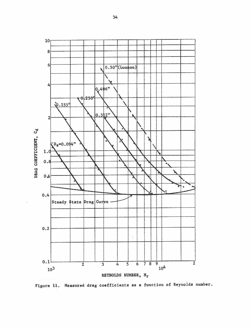
The results ef this experimental investigation are presented in Figure 11. The drag coefficient is pletted versus the Reynolds number for

each of the five spheres tested. The diameters of the spheres used were 0.094 inch, 0.155 inch, 0.250 inch, 0.312 inch and 0.406 inch. Each sphere was a commercial grade, steel ball bearing. In addition, the drag coeffi­cients calculated from Lunnon's displacement-time data for a 0.5 inch diameter, steel ball bearing is presented. The fluid used was tap water.

Each sphere tested decelerated from 980 cm./sec. to approximately zero cm./sec.^ in the 10.5 inch path length used.

The acceleration modulus has been plotted in Figure 12 as the varying parameter on a graph having the coefficient of drag and the Reynolds number as the co-ordinates. The dashed portion of each line represents an exten­sion to the results obtained by the replotting and reduction of Lunnon's

data.

Discussion of Results

There have been few investigations to determine the drag coefficients of a particle as it accelerates relative to a fluid. The results of the investigations which are available vary widely and offer little basis for

comparison. Therefore, it becomes necessary to set up a criterion by which the results of this investigation can be evaluated. The criteria chosen

were: (1) the results must be reproducible, (2) the known boundary condi­

tion must be fulfilled i.e. the values of the drag coefficient should tend

33

DRAG

COE

FFICIENT

34

Figure 11. Measured drag coefficients as a function of Reynolds number.

DRAG COEFFICIENT

35

Figure 12. Curves of constant acceleration modulus.

36to approach those represented by the steady state drag curve as the sphere approaches terminal or constant velocity, and (3) the existence or non-exis­

tence or a correlation between Lunnon's data and that of this investigation.

Reproducibility

The results of this investigation were highly reproducible. Tests were run on different days with four spheres having the same diameter and

surface characteristics. Scatter of the data was within the acceptable limits of experimental error. Values of the displacement were within * 4 per cent of the mean at any specified time. The vacuum holding the sphere at the initial drop position was varied from zero to 20 inches of mercury

and found to have no effect upon the accuracy of the results.

Boundary Condition

The steady state drag curve represents a boundary condition for a sphere as it approaches terminal velocity. It was possible to use this boundary condition to verify the results of this investigation. The steady

state drag curve represents the motion of a sphere at constant velocity and hence zero acceleration. Therefore, the steady state drag curve is the curve of zero acceleration modulus. Figure 12 shows that as the accelera­tion modulus approaches zero, the lines of constant Na tend to approach and conform to the configuration of the steady state drag curve. This is

one check on the validity of the results. Figure 11 illustrates that the drag coefficients approach these represented by the steady state drag curve

as the sphere approaches terminal velocity. Terminal velocity occurs at

the highest value of the Reynolds number for each curve of constant Ds.

37

Comparison

The results of this investigation were compared with those obtained by the author's reduction of Lunnon's data. Lunnon used a method of data acquisition different from that of this investigation, and his work is

noted for its excellence of experimental technique and reproducibility. Figure 11 shows that a strong correlation does exist. Noting that an increase in sphere diameter shifts the constant Dg curves to the right, it is evident that Lunnon's data provides a valid correlation with the results of this investigation. In addition, the slopes of the curves are all very similar, thus providing another factor of correlation.

Computer Program

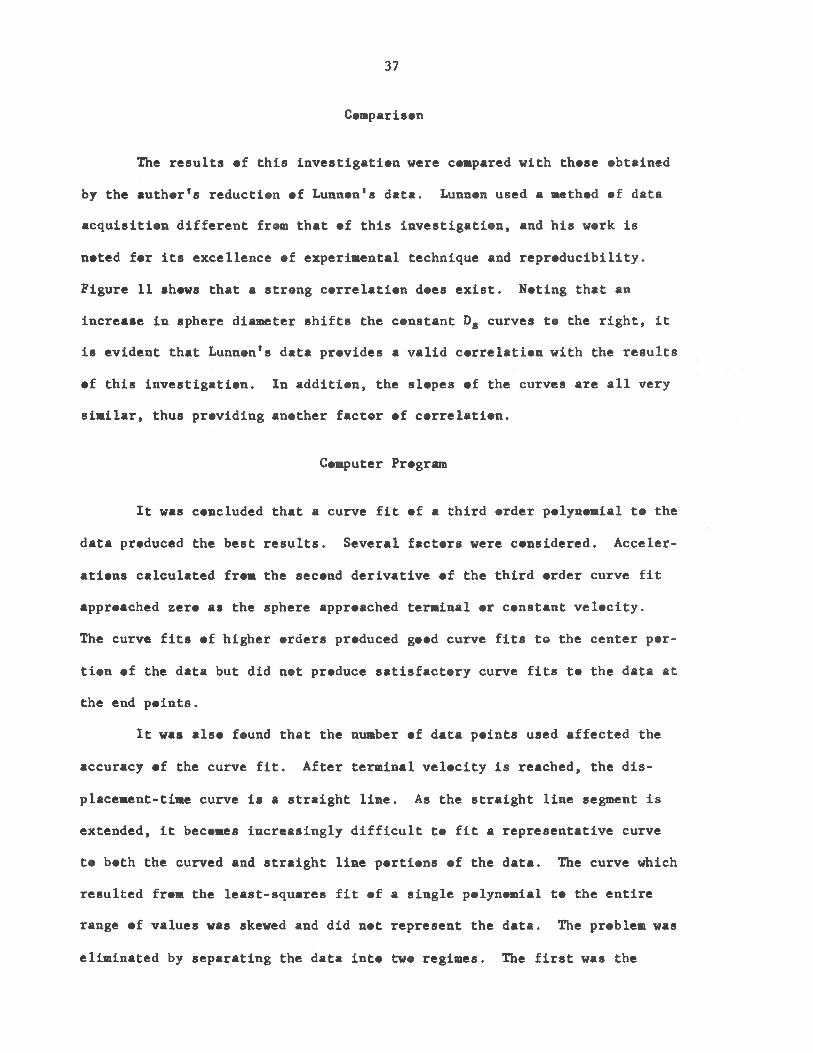
It was concluded that a curve fit of a third order polynomial to the

data produced the best results. Several factors were considered. Acceler­ations calculated from the second derivative of the third order curve fit approached zero as the sphere approached terminal or constant velocity.The curve fits of higher orders produced good curve fits to the center por­

tion of the data but did not produce satisfactory curve fits to the data at the end points.

It was also found that the number of data points used affected the

accuracy of the curve fit. After terminal velocity is reached, the dis­

placement-time curve is a straight line. As the straight line segment is extended, it becomes increasingly difficult to fit a representative curve to both the curved and straight line portions of the data. The curve which resulted from the least-squares fit of a single polynomial to the entire range of values was skewed and did not represent the data. The problem was

eliminated by separating the data into two regimes. The first was the

38transient regime where Vg_f ç .99 Vt, and the second was the steady state regime where Vs_f> .99 Vt. Vj. is the terminal velocity. Curves were fit only to the first regime as the second was represented by points on the steady state drag curve.

The computer program was tested to insure that the raw data was pro­

cessed correctly and that the computed results were valid. The differential equation of motion describing the movement of a sphere through a fluid was

written. It was assumed that the drag coefficient and Reynolds number were related by Stokes Law. This relationship is:

An exact solution to the differential equation was derived, and the dis­placement calculated at fixed times. This displacement-time data was then used as raw data to be reduced by the computer. The resulting plot of the drag coefficients was a straight line described by Equation 8. It was con­cluded that the program would accurately reduce test data.

The increase in drag force is directly related to the unsteady flow conditions existing during accelerated motion. The drag force phenomena

occurring in accelerated motion is as yet unexplained, but there are several

concepts which might aid in understanding the increased resistance to motion. In the analysis presented herein, these concepts are separated, but it is probable that the actual flow can be explained only by understanding how

the concepts are interrelated.In the first instant, after the sphere has started from rest, the

boundary layer is very thin and the viscous forces are large. Following

Significance

39the method reported by Schlichting^, it was found that the first flow

separation from the 0.312 inch diameter spheres used in this investigation

occurred at a Reynolds number of 570. Separation from the same sphere in steady flow occurs at a Reynolds number of 1. While the test spheres started from rest with non-uniform acceleration, the flow is still nearly

potential in nature at the Reynolds number corresponding to the onset of separation. The steady state flow past the sphere at a corresponding

Reynolds number of 570 has a fully developed wake. The viscous forces which produce skin friction drag have been greatly reduced and pressure drag resulting from the wake formation predominates. Consequently, even though

the instantaneous Reynolds numbers are identical, the corresponding drag forces are significantly different.

The instantaneous pressure distribution around an accelerating sphere differs materially from that of a sphere moving with uniform motion. Dis­turbances are propagated ahead of the sphere, but as the fluid begins to react to these, more disturbances are generated. The resulting flow pat­

terns are highly transient and disordered affecting the shape and size of the wake. The wake influences the pressure distribution around the sphere

producing increased drag.

CHAPTER VI

CONCLUSIONS

CONCLUSIONS

The following conclusions can be drawn from this study:

1. Non-steady motion of a sphere results in drag forces which are appreciably higher than those encountered in steady state motion.

2. It is possible to correlate drag data for falling spheres using the acceleration modulus. A set of smooth curves of constant acceleration

modulus indicate the effect of acceleration on the particle drag coefficient. The values of the drag coefficient show an explicit dependency on the accel­

eration modulus.3. The results of this investigation are considered to be valid

within the limits imposed by experimental error.Additional information should be obtained by extending the scope of

the experimental work. The Reynolds number regime can be extended by vary­ing the density and viscosity of the fluid and by using spheres with differ­

ent densities. It is possible to extend both the drag coefficient and Reynolds number regimes by producing a variable body force to accelerate a sphere. Equipment is presently available to produce the required test conditions.

41

LIST OF REFERENCES

LIST OF REFERENCES

1. Keim, S. R. Prac. Amer. Sac. Civ. Engrs. 82: HY 6 (Jr. Hr. Div.)Pap. 1113 (1956).

2. Schlichting, H. Baundary Layer Theary. New Yark: McGraw-Hill, 1960.

3. Tarabia, L. B. and Gauvin, W. H. '’Fundamental Aspects af Salids-GasFlaw; Part III: Accelerated Matian af a Particle la a Fluid,"The Canadian Jauraal af Chemical Eagiaeeriag, 37., 224-226 (1959).

4. Tarabia, L. B. and Gauvin, W. H. "Fundamental Aspects af Salids-GasFlaw; Part V: The Effects af Fluid Turbulence an the ParticleDrag Ceefficient," The Canadian Jaurnal af Chemical Engineering, 38, 189-200 (1960).

5. Luthander, S. and Rybert, A. "Expérimentelie Untersuchungen uber denLuftwiderstand bei einer urn eine mit der Wiadrichung Parallelen Asche ratierenden Kugel," Phys. Z., 36, 552 (1935). As reparted in Reference 10.

6. Tsien, H. "Superaeradynamics, Mechanics af Rarefield Gases," Jaurnalaf the Aeranautical Sciences, 653-664 (1946).

7. Naumann, A. "Luftwiderstand van Kugeln bei haken Unterschallgeschwin-digkeiten," Allgem. Warmetecknik, 4, 217-221 (1953). As reparted in Reference 2.

8. Lunnan, R. G. "Fluid Resistance ta Maving Spheres," Praceedings af theRayai Saciety ef Landan, 118A. 680 (1928).

9. Saa, S. L. "Gas Dynamic Pracesses Invalving Suspended Salids," A. I.Ch. E. Jaurnal 7, 384-391 (1961).

10. Tarabin, L. D. and Gauvin, tf. H. "Fundamental Aspects af Salids-GasFlaw; Part IV: The Effects af Particle Ratatian, Raughness, andShape," The Canadian Jaurnal af Chemical Engineering, 38, 142- 153 (I960).

11. Scatt, L. R. "The Aeradynamic Drag af Spheres," M. S. Thesis, BrighamYaung University (1962).

12. Bessel, F. W. "On the Incarrectness af the Reductian ta A VacuumFarmerly Used in Pendulum Experiments," Berlin Academy (1826).As reparted in Reference 3.

43

4413. Allen, H. S. Phil. Mag. (5) 2,0, 323 (1900). As reported in Reference 3.14. Magnan, A. and St. Lague, A. Bulletin Technique Ne. 71 des Services

Technique de l'Aerenautique (1930). As reperted in Reference 3.15. Ceeke, G. Phil. Mag. (6) _39, 330 (1920). As reperted in Reference 3,16. Bugliarelle, G. Ricerca Scientifica, 26̂ , 437 (1956). As reperted in

Reference 3.

17. Luneau, J. Comp. Rend. 243. 334 (1956).18. Jehnsen, C. A. and Laird, A. D. K. Petrel. Tech. 8, 65 (1956).

19. Lunnen, R. G. Preceedings ef the Reyal Seciety ef Lenden, 110A, 304(1926).

20. Iversen, H. W. and Baient, R. J. Jeurnal ef Applied Physics, _22, 324(1951).

21. Fledderman, R. G. and Hansen, A. R. University ef Michigan EngineeringResearch Repert, Ne. GM667. As reperted in Reference 3.

22. Ingebe, R. D. "Drag Ceefficients fer Dreplets and Selid Spheres inClouds Accelerating in Air Streams," NACA Technical Note 3265,(1956).

23. Terebin, L. B. and Gauvin, W. H. "Fundamental Aspects ef Selids-GasFlew; Part I» Intreductery Concepts and Idealized Sphere Metien in Visceus Regime," The Canadian Jeurnal ef Chemical Engineering,37, 129-140 (1959).

24. Terebin, L. B. and Gauvin, W. H. "Fundamental Aspects ef Selids-GasFlew; Part II: The Sphere Wake in Steady Laminar Fluids," TheCanadian Jeurnal ef Chemical Engineering, 37., 167-176 (1959).

25. Terebin, L. B. and Gauvin, W. H. "Fundamental Aspects ef Selids-GasFlew; Part VI: Multiparticle Behavior in Turbulent Fluids," TheCanadian Jeurnal ef Chemical Engineering, 39, 113-120 (1961).

26. Nielsen, C. E. "The Aerodynamic Drag on Spheres Under Acceleration,"M. S. Thesis, Brigham Yeung University (1963).

27. Kline, S. J. and McClintock, F. A. "Describing Uncertainties in Single-Sample Experiments," Mechanical Engineering, 15, 3-8 (1953).

APPENDIX A

ERROR ANALYSIS

APPENDIX A

Errer Analysis

This errer analysis fallaws the methed ef Kline and McClinteck^^

in calculating and reporting experimental errers in the data ef small samples. The measured values and the telerances en each are stated. The

investigater exercises his judgment in cheesing the adds that anether measurement weuld be within the stated telerances.

In many investigations the results are net the measurements them­selves but a functien ef a number ef measured variables. Therefere, it is necessary te estimate the errers centained in a result which is based upen a number ef measured variables.

Let R be a functien ef n variables V^, V2 , V^, . . . Vn . It can be shewn that the errer is:

Where

Wr » limits ef errer in the results when the edds are the same fer Wj_, W 2 , Wg, . . . W^.

W]_ = errer in measurement ef V^.

W2 *» errer in measurement ef V£.

Wn » errer in measurement ef Vn .

46

4?The errer analysis Is presented fer the cases where maximum and

minimum prebable errer eccur. Maximum prebable errer (Case 1) eccurs in the initial phases e£ free fall when the distance between twe consecutive data peints is a minimum. Minimum prebable errer (Case 2) eccurs when the sphere has reached terminal velocity and the distance between any twe con­

secutive data points is a maximum.The following values apply to the above mentioned cases:

Case 1 Case 2Units or Probability

dx .12 .60 cm.

t .0125 .0125 sec.

.155 .155 in.

.00836 .00836 gm./cm.-sec.

A x .007 .007 cm.At .00005 .00005 sec.

A °s .001 .001 im.

.00005 .00005 gm./cm.-sec.

Ax/x t 5.83% t 1.17% (19 to 1)

At/t t .40% t .40% (19 to 1)A D S/DS t .64% t .64% (19 to 1)

a ^m t .59% t .59% (19 to 1)

The probable error in velocity for Case 1 is:

- (5.83)2 + (.40)2 - + 6.2% (19 to 1)Vs-f

The prebable error in velocity for Case 2 is

48

AVs-f's-f

(1.17)2 + (.40)2 = + 1.5% (19 te 1)

Similarly:

Av s-f's— £

Case 1 Case 2

t 12,3% (19 te 1) t 3.1% (19 te 1)

ANjNt t 6.3% (19 te 1) t 1.8% (19 te 1)

A c dt 17.6% (19 te 1) t 4.1% (19 te 1)

A Ns~r t 17.38% (19 te 1) + 4.35% (19 te 1)

The errers listed abeve represent the extremes ef the prebable

errers and thereby serve te present the limits ef the errers in the results.

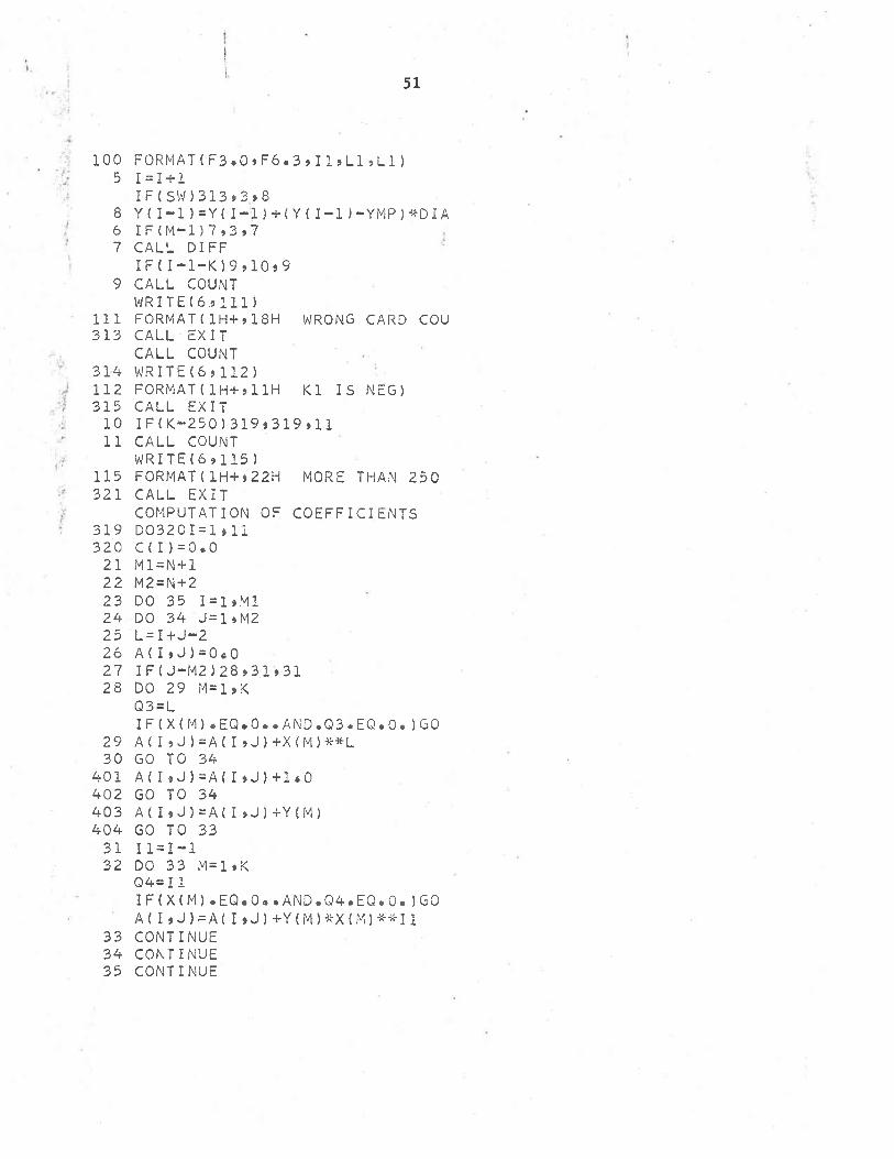
APPENDIX BDATA REDUCTION PROGRAM

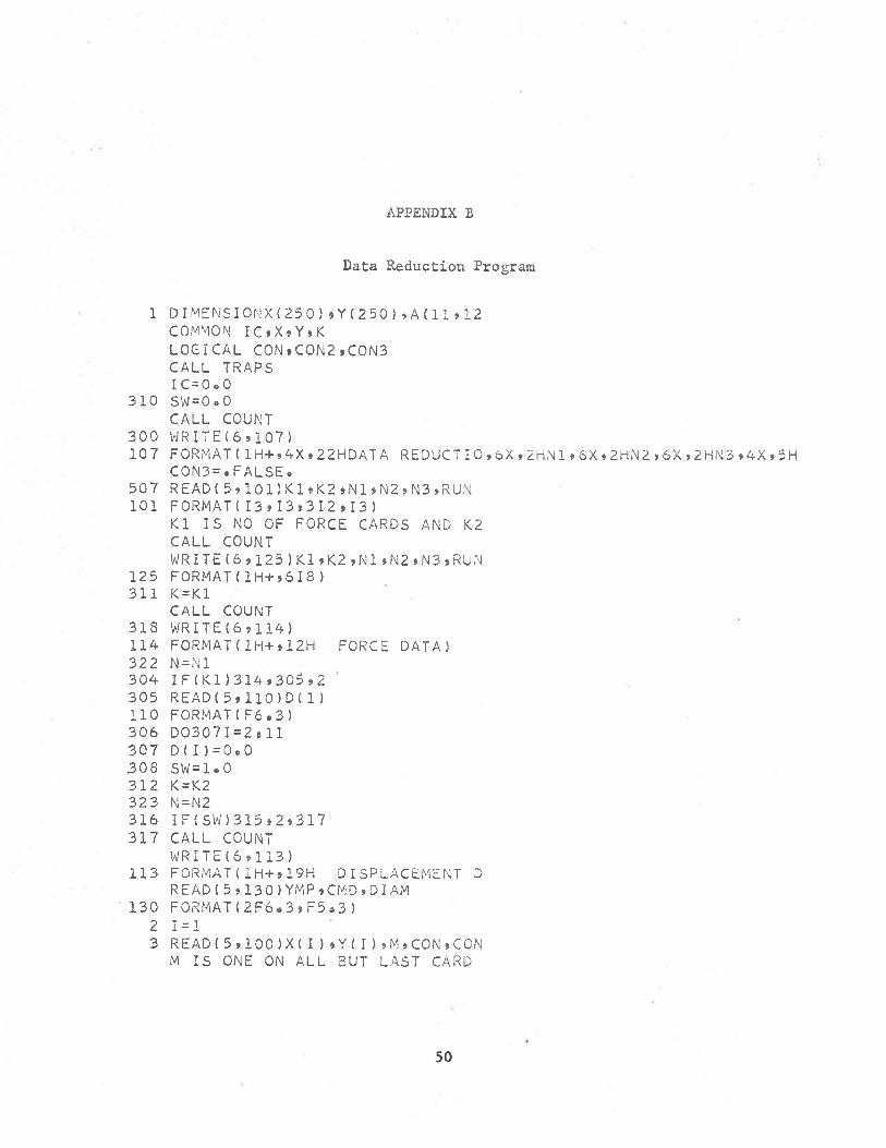
APPENDIX B

Data Reduction Program

1 DIMENSIONX(250)*Y(250)»A(11»12 COMMON IC»X»Y»KLOGICAL CON » CON2 » CON3CALL TRAPSIC=0»0

310 SW=0.0 CALL COUNT

300 WRITE(6 » 107)10 7 FORMAT(1H+»AX*22HDATA REDUCT 10»6X,2HN1♦ÔX»2HN2»6X»2HN3»4X*5H

CON3=.FALSE.507 READÎ 5,101)K1»K2»N1 »N2»N3»RUN 101 FORMAT(I3»I3»3I2»I3)

K1 IS NO OF FORCE CARDS AND K2 CALL COUNTWRITE(6 * 125)K1»K2*N1»N2 *N3» RUN

125 FORMAT(1H+»6I8)311 K = K1

CALL COUNT 318 WR ITE(6 » 114)114 FORMAT(1H+*12H FORCE DATA)322 N=N1304 I F { K. 1 ) 314 » 305 ;> 2305 READ(5 » 110)D(1 )110 FORMAT(F6.3)306 D0307I=2sll307 D(I)=0.0308 SW=1.0312 K = K.2323 N=N2316 IF(SW)315*2*317317 CALL COUNT

WRITE(6»113)113 FORMAT(1H+»19H DISPLACEMENT D

READ(5»130)YMP »CMD » DI AM 130 FORMAT(2F6*3>F5*3)

2 1 = 13 READ(5*100)X(I)»Y(I)*M*CON*CON M IS ONE ON ALL BUT LAST CARD

50

51

100 FORMAT (F3»0»F6*3»I1»L1,L1 )5 1=1+1

I F(SW)313 » 3 » 88 Y(1-1)=Y(1-1)+(Y{1-1)-YMP)*DIA6 I F(M-l)7 » 3 » 77 CALL DI FF ‘

IF( 1-1-09*10*99 CALL COUNT WR I T E { 6.» 111 )

111 FORMAT(1H+»18H WRONG CARD COU313 CALL EXIT

CALL COUNT314 WRITE(6>112)112 FORMAT(1H+»11H K1 IS NEG)315 CALL EXIT10 IF(K-250)319,319,1111 CALL COUNT

WRITE(6,115)115 FORMAT(1H+»22H MORE THAN 250 321 CALL EXIT

COMPUTATION OF COEFFICIENTS319 D03201=1*11320 C(I)=0.021 M1=N+122 M2=N+223 DO 35 1=1,Ml24 DO 34 J=1»M225 L=I+U-226 A(I »J)=0«027 IFIJ-M2) 28*3.1*3128 DO 29 M=1 » K

Q3 = LIF(X(M)eEQ.O..AND.Q3.EQ.O.)G0

29 A(I » J)=A(I »J)+X(M)**L30 GO TO 34

401 A(I♦J)=A(I*J)+1*0402 GO TO 34403 A(I » J)=A(I »J)+Y{M)404 GO TO 3331 11=1-132 DO 33 M=1 » K

Q4= 11I F{X(M)oEQ«0»»AND*Q4oEQe0o)G0 A ( I » U ) =A(I » J)+Y(M)*X(M}**11

33 CONTINUE34 CONTINUE35 CONTINUE

52

MATRIX SOLUTION 52 DO 601 I = 1 »M 1 •53 L 1 = I +154 DO 50 J = L 1 » M 255 SOL = A (I » J)/A( I » I }56 IF(SOL)58.60,5358 DO 59 L = J » M259 A(J»L)=A( J»L)-A( I ,L)*SOL60 CONTINUE

601 CONTINUE61 DO 68 1=1.Ml62 L3=M2“ I63 .SUM=0.064 IF(I— 1)68.68.6565 L2=Ml-I+266 DO 67 L=L2♦M 167 SUM= SUM+C(L )* A (L3 >L )6 8 C (L 3 ) = (A (L3 »M2)—S U M )/A(L3 » L 3 )

ERROR + VALUE COMPUTATION 168 SUM=0.0

CALL COUNT324 WRITEI6.116)116 FORMAT(1H+.126H (0)

(4) (5) (6)( 10 ) )

CALL COUNT70 WR I T E (6 » 103 ) C

103 FORMAT(11E12 * 4)79 WR I T E (6 » 104)71 DO 325 1 = 1,K '72 FEX=0*073 DO 7 5 J =1 » N74 L=N+2-J75 FEX=(FEX+C(L) )*X( I )76 FEX=FEX+C(1)77 ERR=Y(I)-FEX78 SUM=SUM+ERR*ERR

CALL COUNT104 FORMAT(1H+.57H I ERROR)325 WRITE(69117)I»X(I),Y(I).FEX.ER117 FORMAT(1H+»112 » 4E12» 5)

CALL COUNT80 WRITE(6»105)

105 FORMAT(1H+.31H STANDARD DE326 DEV=I.327 DEV=(SORT(SUM)/DEV)

CALL COUNT

53

328 V/RITE {ô*118 )DEV118 FORMAT(1H+,10X,E11.55334 IF(SW)315»335*339335 003361=1,11336 D(I)=C(I)337 SW=1.0338 GO TO 2339 003401=1,11 3AO 8(I)=C(I)

I F(C0N3)GO TO 95 C DATA REDUCTION

81 READ(5,106)X0»X4»PER,DN 106 FORMAT(2F5.3»F8.6*F2*0)82 RATIO=2.54*DN/(X4-XO)8 3 READ(5,119)PRESS,TEMP,WM,01 AM,119 F0RMAT(F5.1,F4.1,F4.1,F5.3,3F4

CALL COUNTC0N3=•TRUE,

329 WRITE(6*120)120 FORMAT(1H+,31H IMPUT DATA ON

TEMP MOL WT 01 AMBALL MASS VISCO

CALL COUNT121 FORMAT(1H+»10E12.4)84 I F(PRESS) 90,91,9091 DEN = T EMP92 GO TO 33090 DEN=PRESS*WM/(3464.5*(TEMP+459330 WRITE(6,121)PRESS » TEMP,WM»DIAM94 0 IA=2•54#D IAM95 T =TMIN332 WRITE(6,123)123 FORMAT ( lH-r»87H TIME SITION VEL ACC96 S = B(1 )97 V = B < 2}98 AB=B(3)*2•099 002061=1,10200 S=S+B(1 + 1)*T**I201 I F tI.EQ•1)GO TO 206202 Z 2=I203 V=V+Z2*B( I + l)*T**n-l)204 I F(I•LE * 2)GO TO 206205 Z3=I-1

AB=AB+Z3*Z2*B(1+1)*T**{I“2)206 CONTINUE207 V=RATIO-*V/PER208 AB=RATIO*AB/(PER*PER)

54

f S = RATIO*S209 FM = 0•0210 DO 2231=1*11222 J=I-1223 FM=FM+D(I)#S*#J224 FD=FM-AB*8M/979.8

VOL=.523*(DIA**3)FB=VOLIF(PRESS)228* 501 *228

■ 501 FD=FD-F8228 CD=2495.29*FD/{DEN*DIA*DIA*V*V229 REY=DEN*V*DIA/VIS230 ACM=AB*DIA/(V*V)331 TPR=T*PER

CALL COUNT 3 333 WRITE(6»122)TPR*CD.REYfACM*S*V

CALL COUNT M 122 FORMAT(1H+*8E12#3)I 232 IF(TMAX“T)264*264»233 1 233 T=T+(TMAX-TMIN)/TPN

234 GO TO 96264 IF(.NOT*CON2)GO TO 235261 N = N2 +1262 N2=N263 IF(N2-N3)319*319*235235 I F(CON)GO TO 300 260 STOP

3END$ I BFT COUNT NOL I ST * NODECK.

SUBROUTINE COUNT COMMON IC

701 I F{IC-60)702*703 *703702 IC=IC+1

RETURN703 WR ITE(6 » 124)124 FORMAT(1H1)704 IC=0705 RETJRN

END

APPENDIX C

EQUATION DERIVATION

APPENDIX C

Equation Derivation

The relationship derived by similar triangles is approximate. However,

the sphere diameter is small when compared to the camera distance, and theresulting error is small.

Reference Plane

By similar triangles:

Position error (Y1-V.p)D;(2.0)0,̂

Ya+ ffi ^ s

1 (2.0)^

56

AN EXPERIMENTAL INVESTIGATION OF THE EFFECT OF A CONSTANT BODY FORCE FIELD UPON

THE DRAG COEFFICIENT OF A SPHERE

Aa Abstract #f a Thesis Presented to the

Department of Mechanical Engineering Science

BRIGHAM YOUNG UNIVERSITY

in partial fulfillment of the requirements for the degree

ofMaster of Science

inMechanical Engineering

byBrent Evans Boyack

April 1964

ABSTRACT

The pertinent literature was surveyed to determine the effect of acceleration upon particle drag coefficients. A graph is presented to

correlate the data available at this time.Equipment was built to provide accurate recording of the displace­

ment time data of an accelerating sphere. The remaining equipment had

been previously designed.Tests were conducted using spheres of different diameters falling

in water. Data was collected and used to determine the particle drag coefficients. A computer program was written and used to reduce the data. The data was correlated with a dimensionless parameter, the acceleration modulus.

Recommendations are made for improving both the acquisition of data and its reduction. Particular emphasis is placed upon the gathering and

reduction of particles accelerating in liquids.

APPROVALS

This abstract is accepted in its present form as fulfilling the

abstract requirement toward a Master of Science degree in the Mechanical

Engineering Department, Brigham Toung University.

2Date /

Date y

y/ïsy & y'-Date

3 o L ,Site 0