ACADEMY OF ACCOUNTING AND FINANCIAL STUDIES JOURNAL · ACADEMY OF ACCOUNTING AND FINANCIAL STUDIES...
162
Volume 15, Number 4 Print ISSN: 1096-3685 PDF ISSN: 1528-2635 ACADEMY OF ACCOUNTING AND FINANCIAL STUDIES JOURNAL Mahmut Yardimcioglu Kahramanmaras Sutcu Imam University Editor The Academy of Accounting and Financial Studies Journal is owned and published by the DreamCatchers Group, LLC. Editorial content is under the control of the Allied Academies, Inc., a non-profit association of scholars, whose purpose is to support and encourage research and the sharing and exchange of ideas and insights throughout the world.
Transcript of ACADEMY OF ACCOUNTING AND FINANCIAL STUDIES JOURNAL · ACADEMY OF ACCOUNTING AND FINANCIAL STUDIES...

Volume 15, Number 4 Print ISSN: 1096-3685 PDF ISSN: 1528-2635
ACADEMY OF ACCOUNTING AND FINANCIAL STUDIES JOURNAL
Mahmut Yardimcioglu Kahramanmaras Sutcu Imam University
Editor
The Academy of Accounting and Financial Studies Journal is owned and published by the DreamCatchers Group, LLC. Editorial content is under the control of the Allied Academies, Inc., a non-profit association of scholars, whose purpose is to support and encourage research and the sharing and exchange of ideas and insights throughout the world.

Page ii
Academy of Accounting and Financial Studies Journal, Volume 15, Number 4, 2011
Authors execute a publication permission agreement and assume all liabilities. Neither the DreamCatchers Group nor Allied Academies is responsible for the content of the individual manuscripts. Any omissions or errors are the sole responsibility of the authors. The Editorial Board is responsible for the selection of manuscripts for publication from among those submitted for consideration. The Publishers accept final manuscripts in digital form and make adjustments solely for the purposes of pagination and organization.
The Academy of Accounting and Financial Studies Journal is owned and published by the DreamCatchers Group, LLC, PO Box 1708, Arden, NC 28704, USA. Those interested in communicating with the Journal, should contact the Executive Director of the Allied Academies at [email protected].
Copyright 2011 by the DreamCatchers Group, LLC, Arden NC, USA

Page iii
Academy of Accounting and Financial Studies Journal, Volume 15, Number 4, 2011
EDITORIAL REVIEW BOARD MEMBERS
Thomas T. Amlie Penn State University-Harrisburg Harrisburg, Pennsylvania
Agu Ananaba Atlanta Metropolitan College Atlanta, Georgia
Manoj Anand Indian Institute of Management Pigdamber, Rau, India
Ali Azad United Arab Emirates University United Arab Emirates
D'Arcy Becker University of Wisconsin - Eau Claire Eau Claire, Wisconsin
Jan Bell Babson College Wellesley, Massachusetts
Roger J. Best Central Missouri State University Warrensburg, Missouri
Linda Bressler University of Houston-Downtown Houston, Texas
Jim Bush Middle Tennessee State University Murfreesboro, Tennessee
Douglass Cagwin Lander University Greenwood, South Carolina
Richard A.L. Caldarola Troy State University Atlanta, Georgia
Eugene Calvasina Southern University and A & M College Baton Rouge, Louisiana
Askar Choudhury Illinois State University Normal, Illinois
Darla F. Chisholm Sam Houston State University Huntsville, Texas
Natalie Tatiana Churyk Northern Illinois University DeKalb, Illinois
Rafik Z. Elias California State University, Los Angeles Los Angeles, California
James W. DiGabriele Montclair State University Upper Montclair, New Jersey
Richard Fern Eastern Kentucky University Richmond, Kentucky
Peter Frischmann Idaho State University Pocatello, Idaho
Farrell Gean Pepperdine University Malibu, California
Luis Gillman Aerospeed Johannesburg, South Africa
Richard B. Griffin The University of Tennessee at Martin Martin, Tennessee
Marek Gruszczynski Warsaw School of Economics Warsaw, Poland
Mohammed Ashraful Haque Texas A&M University-Texarkana Texarkana, Texas

Page iv
Academy of Accounting and Financial Studies Journal, Volume 15, Number 4, 2011
EDITORIAL REVIEW BOARD MEMBERS
Mahmoud Haj Grambling State University Grambling, Louisiana
Morsheda Hassan Grambling State University Grambling, Louisiana
Richard T. Henage Utah Valley State College Orem, Utah
Rodger Holland Georgia College & State University Milledgeville, Georgia
Kathy Hsu University of Louisiana at Lafayette Lafayette, Louisiana
Shaio Yan Huang Feng Chia University China
Dawn Mead Hukai University of Wisconsin-River Falls River Falls, Wisconsin
Robyn Hulsart Ohio Dominican University Columbus, Ohio
Evelyn C. Hume Longwood University Farmville, Virginia
Tariq H. Ismail Cairo University Cairo, Egypt
Terrance Jalbert University of Hawaii at Hilo Hilo, Hawaii
Marianne James California State University, Los Angeles Los Angeles, California
Jeff Jewell Lipscomb University Nashville, Tennessee
Jongdae Jin University of Maryland-Eastern Shore Princess Anne, Maryland
Ravi Kamath Cleveland State University Cleveland, Ohio
Desti Kannaiah Middlesex University London-Dubai Campus United Arab Emirates
Marla Kraut University of Idaho Moscow, Idaho
Brian Lee Indiana University Kokomo Kokomo, Indiana
C. Angela Letourneau Winthrop University Rock Hill, South Carolina
Treba Marsh Stephen F. Austin State University Nacogdoches, Texas
Richard Mason University of Nevada, Reno Reno, Nevada
Richard Mautz North Carolina A&T State University Greensboro, North Carolina
Rasheed Mblakpo Lagos State University Lagos, Nigeria
Nancy Meade Seattle Pacific University Seattle, Washington

Page v
Academy of Accounting and Financial Studies Journal, Volume 15, Number 4, 2011
EDITORIAL REVIEW BOARD MEMBERS
Christopher Ngassam Virginia State University Petersburg, Virginia
Frank Plewa Idaho State University Pocatello, Idaho
Thomas Pressly Indiana University of Pennsylvania Indiana, Pennsylvania
Hema Rao SUNY-Oswego Oswego, New York
Ida Robinson-Backmon University of Baltimore Baltimore, Maryland
P.N. Saksena Indiana University South Bend South Bend, Indiana
Martha Sale Sam Houston State University Huntsville, Texas
Mukunthan Santhanakrishnan Idaho State University Pocatello, Idaho
Milind Sathye University of Canberra Canberra, Australia
Junaid M. Shaikh Curtin University of Technology Malaysia
Philip Siegel Augusta State University Augusta, Georgia
Mary Tarling Aurora University Aurora, Illinois
Darshan Wadhwa University of Houston-Downtown Houston, Texas
Dan Ward University of Louisiana at Lafayette Lafayette, Louisiana
Suzanne Pinac Ward University of Louisiana at Lafayette Lafayette, Louisiana
Michael Watters Henderson State University Arkadelphia, Arkansas
Clark M. Wheatley Florida International University Miami, Florida
Barry H. Williams King’s College Wilkes-Barre, Pennsylvania
Jan L. Williams University of Baltimore Baltimore, Maryland
Carl N. Wright Virginia State University Petersburg, Virginia

Page vi
Academy of Accounting and Financial Studies Journal, Volume 15, Number 4, 2011
TABLE OF CONTENTS
LETTER FROM THE EDITOR ................................................................................................ VIII THE USEFULNESS OF CONTINGENT CLAIMS ANALYSIS IN PREDICTING CORPORATE CREDIT RATINGS ............................................................................................... 1
Mark P. Bauman, University of Northern Iowa REACTIONS TO THE 2008 ECONOMIC CRISIS AND THE THEORY OF PLANNED BEHAVIOR .............................................................................................................. 17
Valrie Chambers, Texas A&M University-Corpus Christi Bilaye R. Benibo, Texas A&M University-Corpus Christi Marilyn Spencer, Texas A&M University-Corpus Christi
THE IMPACT OF MANDATORY IFRS ADOPTION ON STOCK EXCHANGE LISTINGS: INTERNATIONAL EVIDENCE ...................................................... 31
Fei Han, Robert Morris University Haihong He, California State University, Los Angeles
ADVERSE INTERNAL CONTROL OVER FINANCIAL REPORTING OPINIONS AND AUDITOR DISMISSALS/RESIGNATIONS ................................................. 41
Maya Thevenot, SUNY Fredonia Linda Hall, SUNY Fredonia
THE RELATIONSHIP BETWEEN PROFITABILITY AND THE LEVEL OF COMPLIANCE TO THE INTERNATIONAL FINANCIAL REPORTING STANDARDS (IFRS): AN EMPIRICAL INVESTIGATION ON PUBLICLY LISTED CORPORATIONS IN THE PHILIPPINES ................................................................... 61
Rodiel C. Ferrer, De La Salle University Glenda J. Ferrer, University of Rizal System

Page vii
Academy of Accounting and Financial Studies Journal, Volume 15, Number 4, 2011
FINANCIAL PERFORMANCE OF COMPUTER NETWORK AND INFORMATION TECHNOLOGY SERVICES COMPANIES IN BULL AND BEAR MARKETS ..................... 83
Anne Macy, West Texas A&M University Neil Terry, West Texas A&M University Jean Walker, West Texas A&M University
ANALYSTS’ EARNINGS FORECASTS: IMPLICATIONS FOR MANAGED EARNINGS VIA PENSION EXPENSE ...................................................................................... 99
Paula Diane Parker, University of Southern Mississippi FINANCIAL CRISIS AND SHORT SELLING: DO REGULATORY BANS REALLY WORK? EVIDENCE FROM THE ITALIAN MARKET ......................................... 115
Gianluca Mattarocci, University of Rome “Tor Vergata” Gabriele Sampagnaro, University of Naples “Parthenope”
USING INTELLECTUAL CAPITAL DISCLOSURE AS A FRAMEWORK FOR NONFINANCIAL DISCLOSURES: THE DANISH EXPERIENCE ....................................... 141
Jay Holmen, University of Wisconsin—Eau Claire

Page viii
Academy of Accounting and Financial Studies Journal, Volume 15, Number 4, 2011
LETTER FROM THE EDITOR Welcome to the Academy of Accounting and Financial Studies Journal. The editorial content of this journal is under the control of the Allied Academies, Inc., a non profit association of scholars whose purpose is to encourage and support the advancement and exchange of knowledge, understanding and teaching throughout the world. The mission of the AAFSJ is to publish theoretical and empirical research which can advance the literatures of accountancy and finance. As has been the case with the previous issues of the AAFSJ, the articles contained in this volume have been double blind refereed. The acceptance rate for manuscripts in this issue, 25%, conforms to our editorial policies. The Editor works to foster a supportive, mentoring effort on the part of the referees which will result in encouraging and supporting writers. He will continue to welcome different viewpoints because in differences we find learning; in differences we develop understanding; in differences we gain knowledge and in differences we develop the discipline into a more comprehensive, less esoteric, and dynamic metier. Information about the Allied Academies, the AAFSJ, and our other journals is published on our web site. In addition, we keep the web site updated with the latest activities of the organization. Please visit our site and know that we welcome hearing from you at any time. Mahmut Yardimcioglu Kahramanmaras Sutcu Imam University

Page 1
Academy of Accounting and Financial Studies Journal, Volume 15, Number 4, 2011
THE USEFULNESS OF CONTINGENT CLAIMS ANALYSIS IN PREDICTING CORPORATE
CREDIT RATINGS
Mark P. Bauman, University of Northern Iowa
ABSTRACT
Recent research on credit risk focuses on contingent claims analysis, under which the probability a firm will default on its debt can be estimated using equity market and accounting data. As most of this research focuses on the usefulness of contingent claims analysis in the prediction of default and bankruptcy, relatively little attention has been paid to its use in the prediction of corporate credit ratings. This study utilizes a sample of U.S. manufacturing firms to examine the incremental usefulness of the contingent claims framework for predicting issuer credit ratings, given a set of basic accounting ratios. While the results generally indicate that a distance-to-default (DTD) measure derived from the contingent claims framework provides incremental information, notable exceptions occur with AA and A-rated firms. Further testing reveals that information is lost when the theoretical determinants of default risk are combined into a single DTD measure. These results are consistent with research that finds the contingent claims model less useful for investment grade bonds. Key words: credit ratings, financial ratios, contingent claims analysis, default risk
INTRODUCTION
Academic research on firm credit risk dates back more than 40 years. Initial studies examine the usefulness of primarily accounting-based measures in predicting bankruptcy (Beaver 1966; Altman 1968) and credit ratings (Horrigan 1966; West 1970). Recent research focuses on contingent claims analysis, which is based on the similarity between the payoffs to the owners of a firm and the payoffs to a call option (Black and Scholes 1973; Merton 1974). Using option valuation theory, the probability that a firm will default on its debt can be estimated from equity returns and accounting data (Vasicek 1984).
Most research on the application of contingent claims analysis examines its usefulness in predicting bankruptcy and default. Hillegeist et al. (2004) find that the probability of default derived from the model provides significantly more information for predicting bankruptcy than the accounting-based measures of Altman (1968) and Ohlson (1980). However, they find that accounting-based measures possess incremental information content. Thus, the probability of default is not a sufficient statistic for bankruptcy prediction. With respect to default prediction,

Page 2
Academy of Accounting and Financial Studies Journal, Volume 15, Number 4, 2011
Bharath and Shumway (2008) find that a naïve alternative default probability outperforms the probability estimated from the contingent claims model. Further, Benos and Papanastasopoulos (2007) find that distance to default (DTD) is not a sufficient statistic for default prediction.1
The current study examines the usefulness of the contingent claims model for predicting corporate credit ratings. This is an interesting issue because studies focusing on bankruptcy and default prediction address dichotomous outcomes, in which the goal is to discriminate between firms that will continue as going concerns versus those firms that will succumb to financial distress. In contrast, the outcomes in predicting credit ratings are polychotomous. This setting tests the ability of the contingent claims model to discriminate between firms whose capacity to service debt ranges from extremely strong (AAA rating) through speculative (B rating). Thus, it provides a richer setting in which to examine the usefulness of the model.
Two existing studies examine the contingent claims model and the prediction of credit ratings. Du and Suo (2007) examine whether DTD is a sufficient statistic of equity-market information regarding firm credit quality. In this regard, they find that a linear combination of equity market-based variables better predicts credit ratings than DTD alone. In contrast to Du and Suo (2007), the current study focuses on the incremental usefulness of contingent claims analysis given a set of accounting-based measures. This is important given the well-documented association between accounting data and credit ratings.
In their default prediction study, Benos and Papanastasopoulos (2007) provide preliminary evidence regarding the incremental usefulness of the contingent claims model for predicting credit ratings. Using a sample of 270 firms in 2002, they find that distance to default improves the in-sample fit across all rating categories of a model which also includes financial ratios. The present study expands on this preliminary finding by focusing on out-of-sample predictions of credit ratings over a longer period of time. This is important because the use of a holdout sample provides a stronger test of a model's predictive validity and value, than testing the model on the same data set on which it was developed. Contrary to Benos and Papanastasopoulos (2007), the current study finds evidence that the addition of DTD in an accounting-based model does not improve predictions across all rating categories.
This study utilizes a sample of U.S. manufacturing firms to compare the out-of-sample predictive ability of a model based exclusively on reported accounting data to an expanded model that includes a distance-to-default measure from the contingent claims framework. Overall, the model including distance to default correctly predicts a significantly greater percentage of credit ratings and more frequently predicts a rating that is within one rating category. However, the model does not consistently outperform the accounting-only model across all credit rating categories. For firms with issuer ratings of AA, the model including distance to default correctly predicts a greater percentage of credit ratings, but this difference is not statistically significant. For firms with issuer ratings of A, the accounting-only model correctly predicts a greater percentage of ratings. This is consistent with research that finds the contingent claims model less useful for investment grade bonds (Jones et al. 1984; Eom et al.

Page 3
Academy of Accounting and Financial Studies Journal, Volume 15, Number 4, 2011
2004). Additional analysis reveals that the results for AA and A-rated issuers do not imply that information from the contingent claims model is not incrementally informative. In this regard, a third model, which substitutes a linear combination of equity market-related inputs to the contingent claims model in place of DTD, generally provides the most accurate predictions. Thus, it appears that information is lost when the theoretical determinants of default risk are combined into a single DTD measure.
BACKGROUND AND RESEARCH DESIGN Background
Contingent claims analysis is based on the similarity between the payoffs to the owners of a firm and the payoffs to a call option (Black and Scholes 1973; Merton 1974). When the value of a firm’s assets drops below the value of its liabilities (i.e., the strike price), owners can default on the debt (i.e., let the option expire). As the likelihood of default is implicit in the value of the option, it can be empirically estimated from an option pricing model (Vasicek 1984). The equation for valuing a firm’s equity (VE) as a European call option on the value of its assets, after adjusting for dividends, is:2
,)Ve(1)N(dXe)N(deVV AδT
2rT
1δT
AE−−− −+−= (1)
where ( ) ( )( ) .Tσdd,
TσT/2σδr/XVlnd A12
A
2AA
1 −=+−+
= (2)
In the above expressions, VA represents the current market value of assets, δ is the continuous dividend rate (expressed in terms of VA), X is the face value of debt maturing at time T, N is the cumulative standard normal distribution function, r is the continuously-compounded risk-free rate of interest, and σA is the standard deviation of asset returns. The model assumes that the natural log of future asset values is distributed as:
,tσt,2σδμ)ln(VN 2
A
2A
A⎥⎥⎦
⎤
⎢⎢⎣
⎡⎟⎟⎠
⎞⎜⎜⎝
⎛−−+ (3)
where µ is the continuously-compounded expected market return on assets. The estimated probability of default is determined based on the distance to default
(DTD): ( )
.Tσ
/2))T(σδ(μ/XVlnDTDA
2AA −−+
= (4)

Page 4
Academy of Accounting and Financial Studies Journal, Volume 15, Number 4, 2011
Given a firm’s current asset value and its expected volatility, a frequency distribution of asset values at time T can be estimated. DTD measures the number of standard deviation moves required to bring the expected value of a firm’s assets below the default point, X.3 As such, DTD provides an intuitive, theoretically-consistent measure of default risk. Figure 1 provides a graphical depiction of the model. In this study, DTD is computed using the SAS code provided by Hillegeist et al. (2004).4
Figure 1: Graphical Depiction of the Contingent Claims Model
Assuming that asset value follows a lognormal process, a distribution of possible asset values at time T can be estimated. If asset value at time T falls below the default point, the equity holders are assumed to exercise their limited liability rights and surrender ownership to the debtholders. The distance to default measures the ‘margin of safety’ between expected asset value and the default point.
The present study examines the usefulness of contingent claims analysis in predicting corporate credit ratings. This is an important issue because credit ratings assume a significant role in financial markets and there are numerous reasons for market participants to predict ratings (White et al. 2003). Two existing studies examine the contingent claims model and the prediction of credit ratings. Du and Suo (2007) examine whether DTD is a sufficient statistic of equity-market information regarding firm credit quality. In this regard, they find that a linear combination of equity market-based variables better predicts credit ratings than DTD alone.5 They further demonstrate that credit-quality information contained in the market value of equity is not fully utilized in the contingent claims model. In contrast to Du and Suo (2007), the current study focuses on the incremental usefulness of contingent claims analysis given a set of accounting-based measures. While issuer credit ratings should reflect the probability of default, they are more generally intended to reflect an obligor's capacity and willingness to meet its financial commitments.6 For this reason, it is expected that – even in the presence of DTD – accounting data will retain its association with credit ratings as documented in prior research.
In their default prediction study, Benos and Papanastasopoulos (2007) provide some preliminary evidence regarding the incremental usefulness of the contingent claims model for predicting credit ratings. Using a sample of 270 firms in 2002, they find that distance to default

Page 5
Academy of Accounting and Financial Studies Journal, Volume 15, Number 4, 2011
improves the in-sample fit of a model which also includes financial ratios. The present study expands on this preliminary finding. First, it focuses on out-of-sample predictions of credit ratings. This is important because the use of a holdout sample provides a stronger test of a model's predictive validity and value, than testing the model on the same data set on which it was developed. The present study covers a longer period of time (17 years) and a greater number of firms (the holdout sample includes more than 6,000 firm-year observations), increasing the external validity of the results. Second, additional insights are obtained by estimating a model combining accounting variables with a linear combination of equity market-based variables.
A priori, it is not clear whether a model including DTD and accounting variables will significantly outperform an accounting-only model across all credit rating categories. Since DTD is derived from equity prices, it reflects information from sources outside the financial statements. Thus, to the extent that DTD reflects additional, non-accounting information used in the credit rating process, its inclusion should result in superior predictive performance. However, existing research on corporate bond pricing suggests that the incremental usefulness of contingent claims analysis may vary by creditworthiness. Jones et al. (1984) test the Merton model against a naïve model that assumes firm value is sufficiently large as to make all debt riskless. For investment grade bonds, they find that the Merton model is indistinguishable from the naïve model. In contrast, the Merton model has incremental explanatory power for the prices of non-investment grade bonds. Eom et al. (2004) find that the Merton model predicts yield spreads that are systematically too low for investment grade bonds.7 However, predicted spreads for non-investment grade bonds are, on average, considerably more accurate. Thus, the incremental usefulness of DTD may be attenuated for investment-grade firms. Ultimately, the incremental predictive ability is an empirical question. Research Design
The empirical analysis focuses on the relative predictive ability of alternative credit rating
models. Accordingly, a maintained assumption is that credit ratings are accurate measures of creditworthiness. The first model utilizes only reported financial accounting variables to explain observed credit ratings
Credit rating = f(COV, ROA, VOL, LEV, SIZE), (ACCT)
where COV is interest coverage, ROA is return on assets, VOL is the volatility of ROA, LEV is leverage, and SIZE is firm size. These variables are chosen based on a review of recent research (e.g., Hann et al. 2007; UBS 2004).8 Computation of all model variables is described in the Appendix. In addition to accounting variables, the second model includes a distance to default (DTD) derived from the contingent claims model

Page 6
Academy of Accounting and Financial Studies Journal, Volume 15, Number 4, 2011
Credit rating = f(COV, ROA, VOL, LEV, SIZE, DTD). (ACCT-CC) As discussed above, DTD is computed following Hillegeist et al. (2004). The tabulated
results are based on setting the default point equal to the sum of (1) debt in current liabilities, plus (2) 50% of long-term debt.9 Consistent with existing research, the default horizon, T, is set to 1 year.10
Data is collected for the period 1986-2008, which is divided into 17 annual estimation periods from 1992-2008. To provide for more efficient estimation, five years of annual data are pooled for each estimation period. Coefficient estimates are obtained from an ordered probit model regressing actual issuer credit ratings on financial measures. These coefficient estimates are then used to predict credit ratings for the following year. For example, observed credit ratings for 2003-2007 are regressed on financial variables for 2002-2006. The coefficients from this pooled estimation are then used to predict ratings for 2008. To assess the relative performance of the models, the most probable ratings from the ordered probit model are compared to the actual ratings. Two metrics are examined: (1) the percent of actual ratings correctly predicted, and (2) the percent of predicted ratings within one rating category of the actual rating. Comparisons are made on an overall basis and by individual rating category. Statistical significance is assessed using the McNemar (1947) test, a nonparametric test for analyzing frequency data for paired samples.11
SAMPLE AND DATA
The sample is selected from all U.S. manufacturing firms (SIC 2000-3999) with Standard
& Poor’s issuer credit ratings available in the Compustat database during the period 1986-2008. Limiting the sample to the manufacturing sector is intended to increase inter-firm comparability of financial ratios. Financial ratios are computed as 3-year averages, except that volatility (standard deviation) of return on assets is measured over a 5-year period.12 The most restrictive data requirement for computing DTD is the need for one year of daily equity returns from the CRSP database. As a result of these data requirements, the estimation sample consists of 7,775 firm-year observations for 955 separate firms.13 The holdout sample, which consists of observations from the period 1992-2008, includes 6,284 firm-year observations (886 separate firms). Table 1 (Panel A) presents a frequency distribution of credit ratings for the estimation sample compared to all U.S. manufacturers in the Compustat database. It is evident that the firms without sufficient data are more likely to have lower credit ratings. For example, while 21.3% of manufacturers in Compustat have a credit rating of B, 11.7% of the sample observations are rated B. This feature of the sample should be considered when generalizing the study’s findings.

Page 7
Academy of Accounting and Financial Studies Journal, Volume 15, Number 4, 2011
Table 1: Descriptive Statistics for Estimation Sample Panel A: Frequency distribution of credit ratings
Estimation Sample All manufacturers Rating # % % AAA 215 2.8 2.6 AA 687 8.8 8.3 A 2,159 27.8 22.8 BBB 2,220 28.5 23.8 BB 1,585 20.4 21.2 B 909 11.7 21.3 7,775 100.0 100.0
Panel B: Financial variables by credit rating Variable Rating Mean sd 25% 50% 75%
COV AAA 18.65 11.40 9.34 15.40 26.02 AA 15.29 16.28 6.07 9.72 17.87 A 9.11 12.50 3.79 5.77 9.21 BBB 6.45 11.60 2.34 3.66 5.74 BB 5.59 12.37 1.54 2.42 4.27 B 5.40 15.91 0.74 1.35 2.59
ROA AAA 0.234 0.208 0.130 0.196 0.258 AA 0.212 0.200 0.115 0.161 0.210 A 0.224 0.259 0.093 0.133 0.202 BBB 0.235 0.307 0.076 0.111 0.255 BB 0.227 0.341 0.057 0.100 0.200 B 0.087 0.238 0.005 0.053 0.101
VOL AAA 0.072 0.139 0.015 0.027 0.049 AA 0.076 0.131 0.016 0.030 0.051 A 0.116 0.176 0.022 0.038 0.081 BBB 0.151 0.213 0.028 0.051 0.183 BB 0.161 0.221 0.034 0.065 0.169 B 0.120 0.150 0.042 0.072 0.130
LEV AAA 0.490 0.138 0.425 0.511 0.562 AA 0.505 0.152 0.413 0.519 0.609 A 0.534 0.166 0.443 0.543 0.647 BBB 0.555 0.179 0.450 0.572 0.663 BB 0.600 0.197 0.483 0.610 0.715 B 0.668 0.231 0.513 0.679 0.811
SALES AAA 23,306 23,356 6,853 13,831 29,889 AA 14,651 17,538 3,033 7,669 18,263 A 6,965 9,805 1,679 3,512 8,055 BBB 3,997 8,194 895 1,786 3,804 BB 1,488 3,372 326 688 1,497 B 795 1,756 141 340 847
DTD AAA 10.09 5.10 6.96 9.26 11.51 AA 8.73 4.05 6.02 7.93 10.19 A 7.52 3.85 5.04 6.70 8.96 BBB 6.28 3.21 3.99 5.47 7.76 BB 4.75 2.94 2.83 4.05 6.09 B 3.19 2.47 1.59 2.57 4.02
Variables: COV=interest coverage, ROA=return on assets, VOL=standard deviation of ROA, LEV=leverage, SALES=net sales, and DTD=distance to default. All variables are as defined in the Appendix.

Page 8
Academy of Accounting and Financial Studies Journal, Volume 15, Number 4, 2011
Panel B of Table 1 presents descriptive statistics for the independent variables used in the models. With few exceptions, the means and quartile values for each variable are monotonically increasing/decreasing in credit rating in the expected direction. Table 2 presents a correlation matrix for all model variables. Two points are noteworthy. First, all of the Pearson and Spearman correlations between RATING and the independent variables have the expected sign. Second, the Pearson and Spearman correlations are generally similar in magnitude. This is attributed to the lack of extreme values.
Table 2: Correlation Matrix for ACCT and ACCT-CC Model Variables RATING COV1 COV2 COV3 ROA VOL LEV SIZE DTD RATING 0.54 0.35 0.04 0.09 -0.09 -0.24 0.64 0.45 COV1 0.54 0.51 0.18 -0.09 -0.19 -0.21 0.33 0.24 COV2 0.45 0.85 0.54 -0.08 -0.31 0.14 0.22 COV3 0.16 0.31 0.53 -0.18 0.05 ROA 0.31 0.32 0.32 0.19 0.85 -0.51 -0.14 0.44 VOL -0.26 -0.27 -0.17 0.33 -0.42 -0.22 0.36 LEV -0.23 -0.27 -0.34 -0.26 -0.49 -0.33 0.15 -0.44 SIZE 0.64 0.31 0.22 0.06 -0.30 0.18 0.16 DTD 0.52 0.30 0.27 0.13 0.58 0.13 -0.41 0.18 Pearson (Spearman) correlation coefficients are presented above (below) the main diagonal. Correlations not significant at the 0.05 level or better are omitted. Variables: RATING=S&P issuer rating for senior debt, COV1-COV3=interest coverage, ROA=return on assets, VOL=standard deviation of ROA, LEV=leverage, SIZE= natural log of net sales, and DTD=distance to default. All variables are as defined in the Appendix.
RESULTS
Coefficients from Estimation Sample
Results from estimating the ACCT and ACCT-CC models are reported in Table 3. The reported coefficients represent the mean of the 17 annual estimations. Statistical significance is assessed using time-series-based standard errors, adjusted for first-order autocorrelation as in Abarbanell and Bernard (2000).
Results for the accounting-only model (ACCT) are reported in the third column. With respect to interest coverage, the mean coefficient on the increment from 0 to 5 is significantly positive (COV1: 0.262, t=15.52). As expected, the coefficient on the increment from 5 to 20 is also positive, but not as large (COV2: 0.042, t=4.33). The coefficient on the increment above 20 is significantly negative, but very small in magnitude (COV3: -0.015, t=-7.79).14 The mean coefficients for return on assets (ROA: 3.406, t=4.75) and firm size (SIZE: 0.754, t=27.88) are significant with the expected positive sign. Finally, the mean coefficients for the two variables expected to have negative signs are significantly negative: volatility of ROA (VOL: -5.053, t=-3.83), and leverage (LEV: -2.360, t=-4.00). Coefficient estimates from the ACCT-CC model, which adds distance to default (DTD) to the ACCT model, are reported in the last column of Table 3. Consistent with expectations, the

Page 9
Academy of Accounting and Financial Studies Journal, Volume 15, Number 4, 2011
mean coefficient on DTD (0.159, t=5.58) is significantly positive. In addition, the mean coefficients for the accounting variables remain statistically significant with the same signs as in the ACCT model. The in-sample fit of the models is compared via a likelihood ratio test. As expected, the ACCT-CC model exhibits significantly greater goodness of fit than the ACCT model for each of the annual estimations.
Table 3: Coefficient Estimates for ACCT and ACCT-CC Credit Rating Prediction Models Variable Predicted sign ACCT ACCT-CC COV1 + 0.262 (15.52) 0.239 (23.64) COV2 + 0.042 (4.33) 0.035 (4.06) COV3 0/- -0.015 (-7.79) -0.013 (-6.53) ROA + 3.406 (4.75) 2.169 (3.17) VOL - -5.053 (-3.83) -4.375 (-3.96) LEV - -2.360 (-4.00) -2.110 (-3.41) SIZE + 0.754 (27.88) 0.753 (26.31) DTD + 0.159 (5.58) Models: ACCT=accounting only; ACCT-CC=accounting/contingent claims. Variables: COV1-COV3=interest coverage, ROA=return on assets, VOL=standard deviation of ROA, LEV=leverage, SIZE=natural log of net sales, and DTD=distance to default. All variables are as defined in the Appendix. The reported coefficients represent the mean of 11 individual pooled estimations of an ordered probit model. Statistical significance is assessed using time-series-based standard errors, adjusted for first-order autocorrelation (Abarbanell and Bernard 2000).
Out-of-Sample Predictions
Results from comparing the out-of-sample predictive ability of the ACCT and ACCT-CC models are presented in Table 4. Overall, the ACCT-CC model correctly predicts a greater percentage of credit ratings (55.7% vs. 53.2% for the ACCT model). In addition, the ACCT-CC model more frequently predicts a rating that is within one rating category (95.9% vs. 94.4%). Both of these differences are significant at better than the 0.001 level.
The remainder of the table presents comparative results by rating category. In terms of ‘% correct,’ the ACCT-CC model significantly outperforms the accounting-only model in all but two rating categories. For AA-rated firms, the ACCT-CC model (41.0% correct) outperforms the ACCT model (39.1%), but this difference is not significant (p=0.207). For A-rated firms, the ACCT model (68.5% correct) significantly outperforms the ACCT-CC model (67.0%) at the 0.073 level. These findings are noteworthy as it is contrary to the in-sample results of Benos and Papanastasopoulos (2007). However, it is consistent with research that finds the Merton model less useful in pricing investment grade bonds (Jones et al. 1984; Eom et al. 2004).15
With respect to ‘% within 1 rating,’ the ACCT-CC model outperforms the ACCT model for firms rated BBB and below. Again, these results are consistent with those of Jones et al. (1984) and Eom et al. (2004).
Taken at face value, the results indicate that, given a set of basic financial statement ratios, distance to default is not always incrementally informative about credit ratings. However, a lack of incremental predictive power for DTD does not imply that information from the

Page 10
Academy of Accounting and Financial Studies Journal, Volume 15, Number 4, 2011
contingent claims framework is not informative. To address this issue, a third model is estimated.
Table 4: Comparison of Predictive Accuracy of ACCT and ACCT-CC Models
Rating Criterion ACCT ACCT-CC Diff p-value Overall % correct 53.2% 55.7% 2.5% <0.001 % within 1 rating 94.4% 95.9% 1.5% <0.001 AAA % correct 33.6% 42.7% 9.1% 0.012 % within 1 rating 91.6% 93.7% 2.1% 0.090 AA % correct 39.1% 41.0% 1.9% 0.207 % within 1 rating 95.9% 96.1% 0.2% 0.369 A % correct 68.5% 67.0% -1.5% 0.073 % within 1 rating 97.1% 97.2% 0.1% 0.438 BBB % correct 50.9% 54.0% 3.1% 0.001 % within 1 rating 96.4% 97.4% 1.0% 0.002 BB % correct 44.2% 48.1% 3.9% 0.001 % within 1 rating 91.3% 94.4% 3.1% <0.001 B % correct 53.3% 60.1% 6.8% 0.001 % within 1 rating 88.2% 92.1% 3.9% <0.001 Models: ACCT=accounting only; ACCT-CC=accounting/contingent claims. Criteria: ‘% correct’=percent of actual ratings correctly predicted; ‘% within 1 rating’=percent of predicted ratings within one rating category of the actual rating. The most probable rating from the ordered probit model is designated as the predicted rating. All p-values are based on the McNemar test.
Additional Analysis
The contingent claims model relies on equity-market related inputs to derive the distance to default. Accordingly, a third model substituting three equity market-based measures in place of DTD is estimated
Credit rating = f(COV, ROA, VOL, LEV, SIZE, SIGE, MVE, MVA_X) , (ACCT-MKT)
where SIGE is the daily standard deviation of stock returns, MVE is the natural log of market value of equity, and MVA_X is the natural log of the ratio of market value of assets to the default point. The addition of these variables follows Du and Suo (2007). Computation of these additional variables is described in the Appendix. Table 5 presents the coefficient estimates from the ACCT-MKT model. The mean coefficients for SIGE (-4.175, t=-6.79), MVE (0.493, t=5.76), and MVA_X (0.116, t=2.73) are all significant with the expected signs. The results for the remaining coefficients are consistent with the other models, except that ROA becomes insignificant (0.632, t=0.98). Based on a likelihood ratio test, the ACCT-MKT model exhibits significantly greater in-sample goodness of fit than the ACCT-CC model in each of the 17 annual estimations.
Table 6 presents comparisons of the out-of-sample predictive ability of the ACCT-CC and ACCT-MKT models. Overall, the ACCT-MKT model exhibits significantly greater ‘% correct’ (59.7% vs. 55.7%) and ‘% within 1 rating’ (97.5% vs. 95.9%). With respect to ‘%

Page 11
Academy of Accounting and Financial Studies Journal, Volume 15, Number 4, 2011
correct’ by rating category, the ACCT-MKT model outperforms the ACCT-CC model by at least 3.3% for all rating categories, although the 5.5% difference for AAA-rated firms is marginally significant (p=0.071). For the ‘% within 1 rating’ metric, the ACCT-MKT model outperforms the ACCT-CC model for all but AAA-rated firms, although the differences are not significant for AAA or B-rated firms.
Table 5: Coefficient Estimates for ACCT-MKT Credit Rating Prediction Model
Variable Predicted sign ACCT-MKT COV1 + 0.185 (16.11) COV2 + 0.045 (5.44) COV3 0/- -0.013 (-8.11) ROA + 0.632 (0.98) VOL - -4.451 (-3.56) LEV - -1.763 (-3.66) SIZE + 0.300 (3.80) SIGE - -4.175 (-6.79) MVE + 0.493 (5.76) MVA_X + 0.116 (2.73) Model: ACCT-MKT=accounting/market. Variables: COV1-COV3=interest coverage, ROA=return on assets, VOL=standard deviation of ROA, LEV=leverage, SIZE=natural log of net sales, SIGE=standard deviation of daily equity returns, MVE=natural log of market value of equity, and MVA_X=natural log of ratio of market value of assets to the default point. All variables are as defined in the Appendix. The reported coefficients represent the mean of 11 individual pooled estimations of an ordered probit model. Statistical significance is assessed using time-series-based standard errors, adjusted for first-order autocorrelation (Abarbanell and Bernard 2000).
Table 6: Comparison of Predictive Accuracy of ACCT-CC and ACCT-MKT Models Rating Criterion ACCT-CC ACCT-MKT Diff p-value Overall % correct 55.7% 59.7% 4.0% <0.001 % within 1 rating 95.9% 97.5% 1.6% <0.001 AAA % correct 42.7% 48.2% 5.5% 0.079 % within 1 rating 93.7% 90.9% -2.8% 0.051 AA % correct 41.0% 50.6% 9.6% <0.001 % within 1 rating 96.1% 98.0% 1.9% 0.003 A % correct 67.0% 70.3% 3.3% <0.001 % within 1 rating 97.2% 98.3% 1.1% 0.001 BBB % correct 54.0% 57.5% 3.5% <0.001 % within 1 rating 97.4% 99.0% 1.6% <0.001 BB % correct 48.1% 51.5% 3.4% 0.008 % within 1 rating 94.4% 97.1% 2.7% <0.001 B % correct 60.1% 64.2% 4.1% 0.004 % within 1 rating 92.1% 93.6% 1.5% 0.058 Models: ACCT-CC=accounting/contingent claims; ACCT-MKT=accounting/market. Criteria: ‘% correct’=percent of actual ratings correctly predicted; ‘% within 1 rating’=percent of predicted ratings within one rating category of the actual rating. The most probable rating from the ordered probit model is designated as the predicted rating. All p-values are based on the McNemar test.
Page 12
Academy of Accounting and Financial Studies Journal, Volume 15, Number 4, 2011
As noted above, the ACCT-CC model does not significantly outperform the accounting-only (ACCT) model for AA-rated firms and underperforms for A-rated firms. In an untabulated test, the predictive ability of the ACCT-MKT and ACCT models is compared. The ACCT-MKT model results in significantly greater ‘% correct’ across all rating categories. With respect to ‘% within 1 rating,’ the ACCT-MKT model significantly outperforms the ACCT model for all but one rating category. For AAA-rated firms, the ACCT model outperforms the ACCT-MKT model by 0.7%, but this difference is not significant. Taken together, the results indicate that the theoretical determinants of default risk from the contingent claims framework are reflected in credit ratings and provide information incremental to that included in a set of basic accounting measures. However, it appears that information is lost when combining these determinants into a single measure of default risk.
CONCLUSION
Recent research on firm credit risk focuses on contingent claims analysis, which is based on the similarity between the payoffs to the owners of a firm and the payoffs to a call option (Black and Scholes 1973; Merton 1974). The current study extends research on the usefulness of the contingent claims model for predicting corporate credit ratings by assessing the incremental usefulness of the contingent claims framework for predicting credit ratings, given a set of basic accounting ratios.
This study compares the predictive ability of a model based exclusively on reported accounting data to an expanded model that includes a distance-to-default (DTD) measure from the contingent claims framework. While the results generally indicate that DTD provides incremental information, notable exceptions occur with AA and A-rated firms. Further testing reveals that information is lost when the theoretical determinants of default risk are combined into a single DTD measure.
END NOTES 1. As described below, DTD measures the number of standard deviation moves required to bring the expected value of a
firm’s assets below its default point. 2. The following description is based on Hillegeist et al. (2004). 3. A probability distribution can be used to convert DTD to a probability of default. For example, in their commercial
application of the contingent claims model, Moody’s KMV uses an empirical distribution based on a proprietary database of the default experience of publicly-traded U.S. companies (Kealhofer 2003). In untabulated tests, sensitivity analysis is performed by substituting the probability of default from the standard normal distribution for DTD. While this generally reduces predictive ability, it does not affect the overall inferences.
4. The program utilizes the following inputs to estimate DTD in three steps: daily standard deviation of stock returns, Treasury bill rate, market value of equity, dividends paid, and a measure of total liabilities. In the first step, the market value of assets (VA) and standard deviation of asset returns (σA) are estimated by simultaneously solving equation (1) and an optimal hedge equation. Next, these values are used to estimate the expected market return on assets (µ). Finally, DTD is computed via equation (4).
Page 13
Academy of Accounting and Financial Studies Journal, Volume 15, Number 4, 2011
5. The market-based variables include the market value of equity (MVE), the standard deviation of equity returns over the past 12 months, and the ratio of MVE to the default point.
6. Issuer ratings reflect a firm’s overall creditworthiness, apart from its ability to repay individual obligations. In contrast, an issue rating relates to a specific financial obligation, a specific class of financial obligations, or a specific financial program.
7. Eom et al. (2004) find that the underprediction of spreads for safer bonds is common to other implementations of the contingent claims model.
8. The specific set of accounting-based measures chosen is probably not important, given the relatively high degree of correlation between alternative measures. For example, in untabulated tests, variables representing operating profit margin and funds flow-to-debt were added. While these variables increased the model’s predictive ability, the coefficients were not of the expected sign, most likely due to collinearity. In all cases examined, the inclusion of additional variables did not affect inferences regarding the relative predictive ability of the models.
9. Sensitivity analysis is performed by setting the default point equal to (a) the sum of current maturities of long-term debt plus 50% of long-term debt (Vassalou and Xing 2004), and (b) total liabilities (Hillegeist et al. 2004). The Vassalou and Xing (2004) measure is expanded to include short-term notes payable based on the following statement by Standard & Poor’s (2008, 43): “Traditional measures focusing on long-term debt have lost much of their significance, because companies rely increasingly on short-term borrowings.” In untabulated tests, there is no significant difference in the predictive ability of the debt-based default points, while using total liabilities results in significantly lower prediction accuracy.
10. Extending the horizon to 5 years does not alter the study’s inferences. 11. The McNemar test is appropriate for use in “before-and-after experiments when the experimenter is interested in the
number of subjects who respond differently after they are exposed to some intervening condition or treatment” (Daniel 1990, p. 165). The test is chosen as the assumptions for alternative tests (e.g., t test and signed rank test) are not met.
12. Averages are used since credit ratings are designed to be valid over the entire business cycle. The use of averages is common in the literature. For example, Kaplan and Urwitz (1979) use 5-year averages, while Blume et al. (1998) use 3-year averages. To reduce the impact of extreme values, independent variables are winsorized as described in the Appendix. There is no effect on the inferences when the analyses are repeated without winsorization.
13. As there are only 78 observations for firms with credit ratings below B-, the sample is limited to firms with ratings between AAA and B-.
14. In Blume et al. (1998), the coefficient for the last increment of interest coverage is also negative, but not statistically significant.
15. To reconcile this issue, in-sample predictions are examined. To conform to Benos and Papanastasopoulos (2007), the ACCT-CC and ACCT models are modified to (1) combine the AAA and AA rating categories, and (2) substitute single-year ratios for 3-year averages. Contrary to the reported out-of-sample results, the in-sample ‘prediction’ rate for the ACCT-CC model exceeds that for the ACCT model by 1.6% (difference significant at the 0.083 level). This emphasizes the importance of out-of-sample testing. It is noted that Benos and Papanastasopoulos (2007) employ an alternative method of computing DTD. This is not likely to be a significant contributory factor because, while the Merton model has been the subject of various extensions, the accuracy of newer models in explaining bond prices remains problematic (Eom et al. 2004).
REFERENCES
Abarbanell, J. and V. Bernard. 2000. Is the U.S. stock market myopic? Journal of Accounting Research 38: 221-242. Altman, E. 1968. Financial ratios, discriminant analysis and the prediction of corporate bankruptcy. Journal of
Finance 23: 589-609. Beaver, W. 1966. Financial ratios as predictors of bankruptcy. Journal of Accounting Research 6: 71-102. Benos, A. and G. Papanastasopoulos. 2007. Extending the Merton model: A hybrid approach to assessing credit
quality. Mathematical and Computer Modelling 46: 47-68. Bharath, S.T. and T. Shumway. 2008. Forecasting default with the Merton distance-to-default model. Review of
Financial Studies 21: 1339-1369.

Page 14
Academy of Accounting and Financial Studies Journal, Volume 15, Number 4, 2011
Black, F. and M. Scholes. 1973. The pricing of options and corporate liabilities. Journal of Political Economy 7: 637-654.
Blume, M.E., F. Lim, and A.C. Mackinlay. 1998. The Declining credit quality of U.S. corporate debt: Myth or reality? Journal of Finance 53: 1389-1413.
Daniel, W.W. 1990. Applied Nonparametric Statistics, 2e. Boston: PWS-Kent Publishing Company. Du, Y. and W. Suo. 2007. Assessing credit quality from the equity market: Can a structural approach forecast credit
ratings? Canadian Journal of Administrative Sciences 24: 212-228. Eom, Y.H., J. Helwege, and J. Huang. 2004. Structural models of corporate bond pricing: An empirical analysis.
The Review of Financial Studies 17: 499-544. Hann, R.N., F. Heflin, and K.R. Subramanayam. 2007. Fair-value pension accounting. Journal of Accounting and
Economics 44: 328-358. Hillegeist, S.A., E.K. Keating, D.P. Cram, and K.G. Lundstedt. 2004. Assessing the probability of bankruptcy.
Review of Accounting Studies 9: 5-34. Horrigan, J. 1966. The determination of long-term credit standing with financial ratios. Journal of Accounting
Research 4 (Supplement): 44-62. Jones, E.P., S.P. Mason, and E. Rosenfeld. 1984. Contingent claims analysis of corporate capital structures: An
empirical investigation. The Journal of Finance 39: 611-625. Kaplan, R.S. and G. Urwitz. 1979. Statistical models of bond ratings: A methodological inquiry. The Journal of
Business 52: 231-261. Kealhofer, S. 2003. Quantifying credit risk I: Default prediction. Financial Analysts Journal 59: 30-44. Merton, R. 1974. On the pricing of corporate debt: The risk structure of interest rates. Journal of Finance 29: 449-
470. McNemar, Q. 1947. Note on the sampling error of the difference between correlated proportions or percentages.
Psychometrika 12: 153-157. Ohlson, J.A. 1980. Financial ratios and the probabilistic prediction of bankruptcy. Journal of Accounting Research
18: 109-131. Standard & Poor’s. 2008. Corporate Ratings Criteria: 2008. New York: The McGraw-Hill Companies. UBS Investment Bank (UBS). 2004. The New World of Credit Ratings. New York: UBS. Vasicek, O.A. 1984. Credit valuation. Unpublished paper, KMV Corporation. Vassalou, M. and Y. Xing. 2004. Default risk in equity returns. Journal of Finance 59: 831-868. West, R.R. 1970. An alternative approach to predicting corporate bond ratings. Journal of Accounting Research 8:
118-125. White, G.I., A.C. Sondhi, and D. Fried. 2003. The Analysis and Use of Financial Statements, 3e. New York: John
Wiley & Sons, Inc.

Page 15
Academy of Accounting and Financial Studies Journal, Volume 15, Number 4, 2011
Appendix: Variable Definitions (Compustat annual data item numbers in parentheses)
Dependent Variable: Credit rating (RATING) RATING is based on Standard & Poor’s issuer rating for long-term senior debt. RATING is coded as follows: 6=AAA, 5=AA (AA+ through AA-) ... and 1=B (B+ through B-). Independent Variables: Accounting-Only (ACCT) Model: Interest coverage (COV1, COV2, COV3) These variables are based on a 3-year average of annual interest coverage (COV), measured as [pretax income (170) + interest expense (15)] divided by [interest expense (15)]. Any negative annual values are set equal to zero; 3-year averages are winsorized at 100. As demonstrated by Blume et al. (1998), the effect of a change in interest coverage decreases as the level of coverage increases. To allow for this nonlinearity, interest coverage enters the model as
3
1COVj
jjα
=∑
where COVj is defined as
COV1 COV2 COV3 0 ≤ COV < 5 COV 0 0 5 ≤ COV < 20 5 COV - 5 0
20 ≤ COV ≤ 100 5 15 COV – 20 For example, a firm with COV of 22 will have COV1=5, COV2=15, and COV3=2. Based on Blume et al.
(1998), it is expected that the coefficients on COV1 and COV2 will be positive, with COV1>COV2. The coefficient on COV3 is expected to be non-positive. Return on assets (ROA): ROA is a 3-year average of [pretax income (170) + interest expense (15)] divided by [total assets (6)], with values winsorized at the 1st and 99th percentiles. Volatility (VOL): VOL is the standard deviation of ROA over the preceding 5-year period, with values winsorized at the 99th percentile. Leverage (LEV): LEV is a 3-year average of [total liabilities (181)] divided by [total assets (6)], with values winsorized at the 99th percentile. Firm size (SIZE): SIZE is a 3-year average of the natural logarithm of net sales (12), with values winsorized at the 99th percentile.
Additional Independent Variable: Accounting/Contingent Claims (ACCT-CC) Model Distance to default (DTD): DTD measures the number of standard deviation moves required to bring expected total asset value to the default point. DTD is computed using the SAS code provided by Hillegeist et al. (2004),

Page 16
Academy of Accounting and Financial Studies Journal, Volume 15, Number 4, 2011
with the default point, X, set equal to debt in current liabilities (34) plus 50% of long-term debt (9) and T=1. Values are winsorized at the 1st and 99th percentiles.
Additional Independent Variables: Accounting/Market (ACCT-MKT) Model Standard deviation of equity returns (SIGE): SIGE is computed as the daily standard deviation of equity returns from the eighth month before fiscal year-end through the fourth month after fiscal year-end. Values are winsorized at the 99th percentile. Market value of equity (MVE): MVE is measured at the end of the fourth month after fiscal year-end. MVE is log-transformed and winsorized at the 99th percentile. Market value of assets-to-default point (MVA_X): MVA_X is measured as the natural log of [MVA ÷ X]. Since MVA is defined as the market value of equity (MVE) plus the book value of debt at the default point (X), MVA_X simplifies to ln[1 + MVE/X]. Values are winsorized at the 99th percentile.

Page 17
Academy of Accounting and Financial Studies Journal, Volume 15, Number 4, 2011
REACTIONS TO THE 2008 ECONOMIC CRISIS AND THE THEORY OF PLANNED BEHAVIOR
Valrie Chambers, Texas A&M University-Corpus Christi Bilaye R. Benibo, Texas A&M University-Corpus Christi Marilyn Spencer, Texas A&M University-Corpus Christi
ABSTRACT
One of the largest economic crises faced by this generation in the United States had
many adults re-thinking their employment and investment strategies. By the early fall of 2008, many Americans saw their financial and real estate portfolios shrink significantly, while others feared that their savings were in jeopardy. All of this psychic pain provided a unique quasi-experiment for attempts to learn about the effects of perceptions on investing and saving behavior. Understanding the psychological factors that determine people’s intent to change jobs or move investments in different economic environments is important for understanding and eventually predicting people’s economic behavior. This study examines a number of factors identified in the Theory of Planned Behavior to understand what motivates peoples’ intentions regarding these behaviors in a time of historical significance. We find evidence that norms drive peoples’ intent to change jobs and investment strategies. Attitude is also a significant predictor of intent to change jobs. Overall, the Theory of Planned Behavior model appears to explain a substantial portion of the variance in intent to reallocate money.
INTRODUCTION
By the early fall of 2008, all mainstream US news media began warning that problems experienced in financial institutions were having a detrimental effect on Wall Street and were threatening the stability of at least some banks. They reported on high level, urgent meetings of the Secretary of the Treasury and the Chairman of the Federal Reserve System with the heads of federal agencies and investment banks. In that environment, many middle income Americans saw the value of their financial portfolios decrease significantly, and others feared that their savings were in jeopardy. All of this psychic pain provided a unique quasi-experiment for attempts to learn about the effects of perceptions on investing and saving behavior.
Peoples’ intentions and actions, in aggregate can shift economic markets, and not always in a good way. A deeper analysis is needed to understand what factors influence intentions and actions. The theory of planned behavior asserts that people think first (intend) and then act. This theory has been successfully applied to predicting actions in a wide variety of decisions and outcomes, including losing weight (Ajzen, 1991) and computer resource center usage by
Page 18
Academy of Accounting and Financial Studies Journal, Volume 15, Number 4, 2011
business students (Taylor and Todd, 1995). In the theory of planned behavior, attitudes, perceived behavioral control, self-efficacy, and behavioral norms are all dependent variables of intent to act, which in turn is a dependent variable to actual behavior. In this paper, we examine its usefulness for predicting how people intend to react (with respect to their employment and investment strategies) to a perceived national economic crisis. In a meta-study of the link between intent and action, Sheppard, et al. (1988) found the link between these two variables to be both significant and robust in size. The rest of the paper is organized as follows: relevant literature concerning the theory of planned behavior is reviewed. Next the research model is presented, the methodology is described, and the results are analyzed. Finally, the findings are discussed, along with implications for economists and future avenues for research are presented.
LITERATURE REVIEW
Neoclassical economic theory assumes “bounded rationality,” meaning that individuals almost always weigh their opportunity costs and choose an action that will increase their utility. Only occasionally will individuals make impulse decisions. Fishbein and Ajzen’s (1975) theory of reasoned action predicts that subjective norms and attitudes are good predictors of intent, which in turn predicts behavior. Sheppard et al. (1988) analyzed 86 Theory of Reasoned Action studies, finding an average correlation of over 0.53 between intention and behavior. Relying on this work, the correlation between intent and action is acknowledged, but not tested, here. The theory of reasoned action evolved into the theory of planned behavior, which adds self-efficacy as a cause of intent (Ajzen, 1985 and Ajzen, 1991). This paper compares the relationships of one traditional dependent variable, intent to act, during a global financial crisis according to the theory of planned behavior, as adapted for the specifics of this financial crisis. Additionally, we control for standard demographic variables, which we expect to have no significant effect.
HYPOTHESES AND MODEL DESIGN Intent to Change Jobs and Intent to Move Money
Intent is the extent to which a person is willing to exert an effort in order to perform a specified behavior (e.g. changing jobs). This paper measures intent to react to the national financial crisis by changing income streams (voluntary employment change) and investment allocation. Respondents were asked for example, on a 5-point scale how true (1= very untrue and 5=very true) was the following statement: “…I intend to move my financial assets from financial markets to cash or “… I intend to move my financial assets from financial markets into banks. The five point scale remains constant for all hypotheses.
Page 19
Academy of Accounting and Financial Studies Journal, Volume 15, Number 4, 2011
Primary Dependent Variables
Perceived behavioral control is the amount of effect that people believe they have on their financial circumstances. A person may want to change jobs, but feel that there are no comparable jobs available. Stated as a hypothesis, perceived behavioral control is expected to have a significant, positive effect on both intents, or:
H1: Int Job = B0 + B1 * PBC H2: Int Invest = B0 + B1 * PBC
Where Int Job is the intent to change jobs, Int Invest is the intent to change one’s
investment portfolio to a more conservative mix of savings and other insured investments, and PBC is perceived behavioral control over one’s financial situation.
Ajzen (1991) found that awareness of other people's opinions produced changes in respondents' intents. Subjective norms are defined here as "the awareness of peers' changing asset allocations (jobs)." Applied to this study, the general construct of subjective norms will be tested to see if significant others' opinions and purported actions affect peoples’ intent to change jobs or reallocate investments. Two measures are: “As a result of current changes in the economy my relatives are moving their financial assets from financial markets into banks” and “As a result of the current changes in the economy my relatives are moving their financial assets from financial markets into cash.” Consistent with the theory of planned behavior, it is anticipated that the relationship between subjective norms and both intents is positive and significant:
H3: Int Job = B0 + B1 * NORM H4: Int Invest = B0 + B1 * NORM
Where NORM measures subjective norms, which is how the respondents’ friends and
family are reacting to the crisis in terms of moving jobs and making their portfolio more conservative.
Ajzen (1991) tested the effect of self-efficacy, which is the amount of confidence one has in his/her own abilities. Consistent with the theory of planned behavior, it is anticipated that the relationship between self-efficacy and both intents is positive and significant:
H5: Int Job = B0 + B1 * SE H6: Int Invest = B0 + B1 * SE
Where self-efficacy is the confidence one has in his/her own ability to change jobs or to
make his/her portfolio mix to more conservative savings accounts.

Page 20
Academy of Accounting and Financial Studies Journal, Volume 15, Number 4, 2011
Ajzen (1991) also tested the effect of affective attitude on intent, finding a significant positive relationship. Attitude can be generally defined as "how favorably or unfavorably the examined behavior is viewed." Attitude is operationalized as participants’ responses to survey questions on how secure they felt about three aspects of their finances: savings accounts, investment funds (stocks and bonds) and incomes from their jobs. Respondents were asked to indicate, for example, how true the following statement was: “I feel that my savings in a bank is secure.” It is anticipated that the relationship between attitude about the economy and both intents is negative and significant:
H7: Int Job = B0 - B1 * ATT H8: Int Invest = B0 - B1 * ATT
Figure 1 – Research Model
Control variables (including age, gender, household income, racial identity, religiosity
and experience) were also tested, with no significant results expected. The model can be expressed pictorially, as shown in Figure 1. Sample and Data Collection
Approximately 458 members of a South Texas university’s students, faculty members, and administrators/staff participated in this survey. Respondents from each of the categories were selected both purposively and on the basis of convenience. For example, those professors teaching classes of over 60 students were more likely to be solicited for permission to administer
Self-Efficacy
Perceived Behavioral
Control
Norms
Attitude
Intent to Move
Money
Intent to Move Job
(-)
(-)
(+)
(+)
(+)
(+) (+)
(+)

Page 21
Academy of Accounting and Financial Studies Journal, Volume 15, Number 4, 2011
the questionnaires in their classes than those with smaller classes. Results for students did not vary significantly from the results of faculty and staff, indicating the fitness of students as subjects. Care was taken to ensure that participating students came from different class standings (freshmen, to graduate) and that faculty and staff from each college in the university was represented. Overall, the sample reflects the general demographic distribution of the university. Unlike students’ questionnaires, however, faculty members, staff and administrators’ questionnaires and Informed Consent Forms were mailed with separate return, self-addressed envelopes.
To explore any possible bias resulting from the use of students, bivariate correlations between demographic data and the independent variables (perceived behavioral control, norms, self-efficacy and attitude) and dependent variables (intent to change job, intent to reallocate investments) were calculated. There were no significant correlations, except as noted in the results section. Based on these results, it appears that demographic factors are generally not significant in explaining intent; therefore, the use of student subjects, whose demographic data may not be reflective of the general population, can provide useful information.
The survey instrument itself was extensive and collected information beyond that pertaining to the Theory of Planned behavior and control variables. Only information pertaining to those constructs was extracted and analyzed here. The survey is shown in Appendix A. Note that some questions are reverse-scaled to protect against positive response bias. Written instructions were included with the instrument to the participants, to assure the confidentiality of participants and stress the voluntary nature of participation.
The strength of the model and the scales used to measure their underlying latent constructs, shown in Figure 1, were assessed by applying partial least squares (PLS) analysis. PLS addresses both the effectiveness of the model and the reliability of the underlying measures simultaneously and has many additional advantages, such as relaxed error and distribution assumptions (Wold, 1982).
RESULTS
The age of the participants ranged from 16 to 71, with a median age of 23. Fifty-nine percent were female. Respondents included those with very little perceived experience to those with more extensive experience. The average participant rated herself as having experience of 3.0 on a 5-point scale. Approximately 71 percent of the respondents live in households with monthly income of at least $2,000, and the average monthly income was $4,818, similar to that of the national average.
In order to assess the construct validity of each measurement item, factor loadings are calculated. A factor loading of 0.70 or greater is considered to be a substantial correlation between the indicator and the latent variable (Chin, 1998). Barclay et al. (1995) recommend a loading of 0.707 or higher but he notes that it is not uncommon for items in newly developed
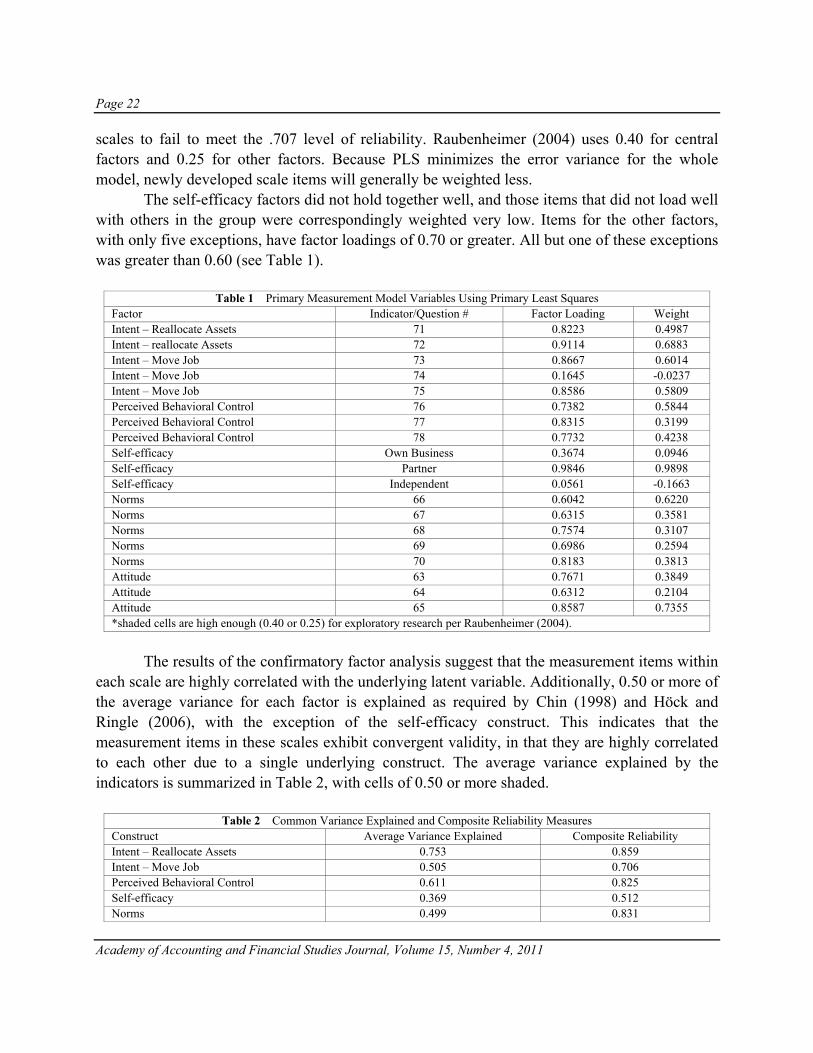
Page 22
Academy of Accounting and Financial Studies Journal, Volume 15, Number 4, 2011
scales to fail to meet the .707 level of reliability. Raubenheimer (2004) uses 0.40 for central factors and 0.25 for other factors. Because PLS minimizes the error variance for the whole model, newly developed scale items will generally be weighted less.
The self-efficacy factors did not hold together well, and those items that did not load well with others in the group were correspondingly weighted very low. Items for the other factors, with only five exceptions, have factor loadings of 0.70 or greater. All but one of these exceptions was greater than 0.60 (see Table 1).
Table 1 Primary Measurement Model Variables Using Primary Least Squares Factor Indicator/Question # Factor Loading Weight Intent – Reallocate Assets 71 0.8223 0.4987 Intent – reallocate Assets 72 0.9114 0.6883 Intent – Move Job 73 0.8667 0.6014 Intent – Move Job 74 0.1645 -0.0237 Intent – Move Job 75 0.8586 0.5809 Perceived Behavioral Control 76 0.7382 0.5844 Perceived Behavioral Control 77 0.8315 0.3199 Perceived Behavioral Control 78 0.7732 0.4238 Self-efficacy Own Business 0.3674 0.0946 Self-efficacy Partner 0.9846 0.9898 Self-efficacy Independent 0.0561 -0.1663 Norms 66 0.6042 0.6220 Norms 67 0.6315 0.3581 Norms 68 0.7574 0.3107 Norms 69 0.6986 0.2594 Norms 70 0.8183 0.3813 Attitude 63 0.7671 0.3849 Attitude 64 0.6312 0.2104 Attitude 65 0.8587 0.7355 *shaded cells are high enough (0.40 or 0.25) for exploratory research per Raubenheimer (2004).
The results of the confirmatory factor analysis suggest that the measurement items within
each scale are highly correlated with the underlying latent variable. Additionally, 0.50 or more of the average variance for each factor is explained as required by Chin (1998) and Höck and Ringle (2006), with the exception of the self-efficacy construct. This indicates that the measurement items in these scales exhibit convergent validity, in that they are highly correlated to each other due to a single underlying construct. The average variance explained by the indicators is summarized in Table 2, with cells of 0.50 or more shaded.
Table 2 Common Variance Explained and Composite Reliability Measures Construct Average Variance Explained Composite Reliability Intent – Reallocate Assets 0.753 0.859 Intent – Move Job 0.505 0.706 Perceived Behavioral Control 0.611 0.825 Self-efficacy 0.369 0.512 Norms 0.499 0.831

Page 23
Academy of Accounting and Financial Studies Journal, Volume 15, Number 4, 2011
To test the reliability of each of the scales, a composite reliability is also presented in Table 2. Except for the self-efficacy construct, each of the reliability statistics generally approaches or exceeds the 0.80 recommended by Nunnally and Bernstein (1994), and exceed 0.60 used by Chin (1998) and Höck and Ringle (2006). These cells are shown as shaded in the table.
The correlations among the latent variables are shown in Table 3, with the numbers presented in the diagonal depicting the square root of the average common variance extracted by the measurement items within the scale (the average inter-item correlation). The correlations among the latent variables are smaller than the square root of the common variance extracted within each scale, demonstrating divergent validity (items within a scale are more significantly related to one another than to items in other scales). Based on the preceding results, the measurements exhibit reasonable validity and reliability.
Table 3 – Correlations among Latent Variables
Construct Intent to Relocate Assests
Intent to Move Job
Perceived Behavioral Control Self-efficacy Norms Attitudes
Intent – Reallocate Assets 0.868 Intent - Move Job 0.19 0.711 Perceived Behavioral Control -0.08 0.071 0.782 Self-efficacy 0.124 0.023 0.02 0.607 Norms 0.592 0.203 -0.081 0.162 0.706 Attitude -0.231 -0.315 0.14 0.049 -0.21 0.758 *The numbers presented in the diagonal depicting the square root of the average common variance extracted by the measurement items within the scale.
The path coefficients to the indicators from the latent variables (epistemic correlations)
are presented in Figure 2. Three path coefficients are significant at α < 0.05 and of the correct sign, supporting hypotheses 3 (Norm to Intent to Move Jobs), 4 (Norm to Intent to Reallocate Assets) and 7 (Attitude to Intent to Move Jobs). All other paths (hypotheses 1, 2, 5, 6 and 8) were insignificant.
Figure 2 – Structural Model Using Primary Least Squares
Significant at α<0.05.
Self-Efficacy
Perceived Behavioral
Control
Norm
Attitude
Intent to Move Money (0.364)
Intent to Move Job
(0.135)
-0.302*
-0.113
0.148
0.011
0.039
0.560
0.125
-0.019

Page 24
Academy of Accounting and Financial Studies Journal, Volume 15, Number 4, 2011
DISCUSSION
A path coefficient greater than 0.20 is meaningful per Chin (1998). Analyses of the results show that norms are a large, significant determinant of whether people intend to reallocate their assets.
Attitude is the significant determinant of whether people intend to move jobs. Norms influence whether one intends to change jobs, but not as much as attitude. The theory of planned behavior appears to be only moderately useful in predicting job turnover in times of financial crisis.
The amount of variance in the endogenous variables explained by the model is represented by the squared multiple correlations of 0.135 for intent to move jobs and 0.364 for intent to reallocate assets. Per Chin (1998) and Höck and Ringle (2006), an R-squared of 0.67 is considered substantial, 0.33 is moderate and 0.19 is weak explanatory power for dependent variables. The model appears to explain a substantial portion of the variance in intent to reallocate money. To determine the usefulness of the research model in Figure 2, the results of this model are compared to those from a simple model, in which norms are the only antecedents to intent to move money in to safer investment vehicles. In the simple model, the path from norms to intent to move money is significant (α < 0.005), the explained variance in the attitude variable is 0.351 and the path size is 0.592. The addition of other independent variables do not add much explanatory power to the model, indicating that in predicting whether people will move out of the stock market and into conservative bank accounts, people are most heavily influenced by the behavior of their peers (norms). They make their investment decisions by following the crowd. Over one-third of people’s investment decisions in a crisis come from referencing the behavior of family and friends, a result that lends credence to the powerful intrusion of social psychology on the otherwise rational man (homo economis).
Indeed, a blended, behavioral economics approach is gathering favor in policy-setting circles (Spiegel, 2009). To test whether the participants are influential on their family and friends rather than the other way around, the model was revised to show causality in the opposite direction and re-tested. The result was significantly worse. It appears that at least with respect to norms, people are following the crowd, not leading it, consistent with the theory of planned behavior, and encouraging a deeper look at collective economic behavior through a social psychology lens.
FURTHER RESEARCH
The effect of norms on individuals’ decisions to move money dominates the findings in this paper. This information is useful and simultaneously consistent with behavioral economic theory and contrary to economic theory portraying each individual investor as a “rational man.” Much of the recent behavioral economic theory centers on how individuals behave. From these

Page 25
Academy of Accounting and Financial Studies Journal, Volume 15, Number 4, 2011
findings, social psychology theory might deserve a second, harder look. Why do people follow the crowd? Economically, how do crowds behave?
Further, if people are following the crowd when making decisions, how should policy makers respond? Should popular opinion alone rule, and if so, should we (how can we) influence the popular opinion in times of economic crisis?
LIMITATIONS
The self-efficacy construct was measured essentially with a single item scale, in that the being a partner in a business modeled well with the theory of planned behavior, but the other measures of independence did not. It is preferable that measurement scales contain multiple, cohesive items. Future research with improved self-efficacy measures might lead to interesting and significant findings.
Finally, actual behavior was not included in the study. This is not a substantial problem because previous studies in the behavioral intentions research stream have supported a strong relationship between intention and actual behavior.
CONCLUSION
In predicting people’s intent to change jobs, our model was weak, but with some significant findings: we find evidence that norms and attitude toward conservative financial investment strategies drive peoples’ intent to change jobs. In predicting people’s intent to move their money to conservative investments, like bank accounts, the model is much more robust, with over 36% of the intent explained by the model. Norms are significant and strongly positive. People intended to react to the global financial crisis the same way their peers did, indicating a strong social aspect to individuals’ plans to handle their personal finances. This finding is important, adding to the growing literature that people are social, not strictly rational investors.
REFERENCES Ajzen, I. (1985). “From Intentions to Actions: A Theory of Planned Behavior,” Action Control - From Cognition to
Behavior, J. Kuhl and J. Beckmann (eds.), (Berlin: Springer-Verlag), 11-39. Ajzen, I. (1991). “The Theory of Planned Behavior,” Organizational Behavior and Human Decision Processes, Vol.
50, 179-211. Barclay, D., R. Thompson, C. Higgins (1995). The partial least squares (PLS) approach to causal modeling: Personal
computer adoption and use as an illustration. Technology Studies,. 285-323. Chin, W.W. (1998). “The Partial Least Squares Approach for Structural Equation Modeling,” In Modern Methods
for Business Research, G.A. Marcoulides, Ed. (Lawrence Erlbaum Associates, Mahwah, NJ). Fishbein, M., and Ajzen, I. (1975). Belief, Attitude, Intention, and Behavior: An Introduction to Theory and
Research, (Addison-Wesley, Reading, MA). Nunally, J.C., and Bernstein, I.H. (1994). Psychometric Theory, (McGraw-Hill, New York), 3rd Edition.

Page 26
Academy of Accounting and Financial Studies Journal, Volume 15, Number 4, 2011
Sheppard, B.H., Hartwick, J., and Warshaw, P.R. (1988). “The Theory of Reasoned Action: A Meta-Analysis of Past Research with Recommendations for Modifications and Future Research,” Journal of Consumer Research, Vol. 15 (December), 325-343.
Spiegel, A. (2009). “Using psychology to save you from yourself.” Nation, June 10, 2009. www.npr.org/templates/story/story.php?storyId=104803094 , retrieved 6/10/2009.
Taylor, S., and Todd, P. (1995). “Understanding Information Technology Usage: A Test of Competing Models,” Information Systems Research, (June), 144-176.
Wold, H. (1982). Soft modeling, the basic design and some extensions.
APPENDIX
Today’s date ______________________________ Read each item and, as honestly as you can, answer the question: “How characteristic or true is this of me?” Circle the appropriate number, using the following scale: 1 = very untrue 2 = untrue 3 = neutral 4 = true 5 = very true DK = don’t know 1. I believe that getting together with one’s friends to party is one of life’s important pleasures. 1 2 3 4 5 2. Familiar childhood sights, sounds, and smells often bring back a flood of wonderful memories. 1 2 3 4 53. Fate determines much in my life. 1 2 3 4 54. I often think of what I should have done differently in my life. 1 2 3 4 55. My decisions are mostly influenced by people and things around me. 1 2 3 4 56. I believe that a person’s day should be planned ahead each morning. 1 2 3 4 57. It gives me pleasure to think about my past. 1 2 3 4 58. I do things impulsively. 1 2 3 4 59. If things don’t get done on time, I don’t worry about it. 1 2 3 4 5
10. When I want to achieve something, I set goals and consider specific means for reaching those goals.
1 2 3 4 5
11. On balance, there is much more good to recall than bad in my past. 1 2 3 4 512. When listening to my favorite music, I often lose all track of time. 1 2 3 4 513. Meeting tomorrow’s deadlines and doing other necessary work come before tonight’s play. 1 2 3 4 514. Since whatever will be will be, it doesn’t really matter what I do. 1 2 3 4 515. I enjoy stories about how things used to be in the “good old times.” 1 2 3 4 516. Painful past experiences keep being replayed in my mind. 1 2 3 4 517. I try to live my life as fully as possible, one day at a time. 1 2 3 4 518. It upsets me to be late for appointments. 1 2 3 4 519. Ideally, I would live each day as if it were my last. 1 2 3 4 520. Happy memories of good times spring readily to mind. 1 2 3 4 521. I meet my obligations to friends and authorities on time. 1 2 3 4 522. I’ve taken my share of abuse and rejection in the past. 1 2 3 4 523. I make decisions on the spur of the moment. 1 2 3 4 524. I take each day as it is rather than try to plan it out. 1 2 3 4 525. The past has too many unpleasant memories that I prefer not to think about. 1 2 3 4 526. It is important to put excitement in my life. 1 2 3 4 527. I’ve made mistakes in the past that I wish I could undo. 1 2 3 4 528. I feel it’s more important to enjoy what you’re doing than to get work done on time. 1 2 3 4 529. I get nostalgic about my childhood. 1 2 3 4 5

Page 27
Academy of Accounting and Financial Studies Journal, Volume 15, Number 4, 2011
Read each item and, as honestly as you can, answer the question: “How characteristic or true is this of me?” Circle the appropriate number, using the following scale: 1 = very untrue 2 = untrue 3 = neutral 4 = true 5 = very true DK = don’t know 30. Before making a decision, I weigh the costs against the benefits. 1 2 3 4 531. Taking risks keeps my life from becoming boring. 1 2 3 4 532. It’s more important for me to enjoy life’s journey than to focus only on the destination. 1 2 3 4 533. Things rarely work out as I expected. 1 2 3 4 534. It’s hard for me to forget unpleasant images of my youth. 1 2 3 4 5
35. It takes joy out of the process and flow of my activities if I have to think about goals, outcomes, and products.
1 2 3 4 5
36. Even when I am enjoying the present, I am drawn back to comparisons with similar past experiences.
1 2 3 4 5
37. You can’t really plan for the future because things change so much. 1 2 3 4 538. My life path is controlled by forces I cannot influence. 1 2 3 4 5
39. It doesn’t make sense to worry about the future, since there is nothing that I can do about it anyway.
1 2 3 4 5
40. I complete projects on time by making steady progress. 1 2 3 4 541. I find myself tuning out when family members talk about the way things used to be. 1 2 3 4 542. I take risks to put excitement in my life. 1 2 3 4 543. I make lists of things to do. 1 2 3 4 544. I often follow my heart more than my head. 1 2 3 4 545. I am able to resist temptations when I know that there is work to be done. 1 2 3 4 546. I find myself getting swept up in the excitement of the moment. 1 2 3 4 547. Life today is too complicated; I would prefer the simpler life of the past. 1 2 3 4 548. I prefer friends who are spontaneous rather than predictable. 1 2 3 4 549. I like family rituals and traditions that are regularly repeated. 1 2 3 4 550. I think about the bad things that have happened to me in the past. 1 2 3 4 551. I keep working at difficult, uninteresting tasks if they will help me get ahead. 1 2 3 4 552. Spending what I earn on pleasures today is better than saving for tomorrow’s security. 1 2 3 4 553. Often luck pays off better than hard work. 1 2 3 4 554. I think about the good things that I have missed out on in my life. 1 2 3 4 555. I like my close relationships to be passionate. 1 2 3 4 556. There will always be time to catch up on my work. 1 2 3 4 5

Page 28
Academy of Accounting and Financial Studies Journal, Volume 15, Number 4, 2011
Read each item and, as honestly as you can, answer the question: “How characteristic or true is this of me?” Circle the appropriate number, using the following scale: 1 = very untrue 2 = untrue 3 = neutral 4 = true 5 = very true DK = don’t know 57. In Fall 2007 I felt that my savings in a bank were secure. 1 2 3 4 5 DK58. In Fall 2007 I felt that my investment funds (stocks & bonds) were secure. 1 2 3 4 5 DK59. In Fall 2007 I felt that my job (source of income) was secure. 1 2 3 4 5 DK60. In August 2008 I felt that my savings in a bank were secure 1 2 3 4 5 DK61. In August 2008 I felt that my investment funds (stocks & bonds) were secure. 1 2 3 4 5 DK62. In August 2008 I felt that my job (source of income) was secure. 1 2 3 4 5 DK63. Today I feel that my savings in a bank is secure. 1 2 3 4 5 DK64. Today I feel that my investment funds (stocks & bonds) are secure. 1 2 3 4 5 DK65. Today I feel that my job (source of income) was secure. 1 2 3 4 5 DK
66. As a result of changes in the economy many of my relatives are moving their financial assets from financial markets into banks.
1 2 3 4 5 DK
67. As a result of changes in the economy many of my relatives are moving their financial assets from financial assets into cash.
1 2 3 4 5 DK
68. As a result of changes in the economy many of my relatives are looking for a new job 1 2 3 4 5 DK69. As a result of changes in the economy many of my relatives are retiring. 1 2 3 4 5 DK70. As a result of changes in the economy many of my relatives are training for a new job. 1 2 3 4 5 DK
71. As a result of changes in the economy many of my relatives are ___________ (please specify and state extent to which it true.
1 2 3 4 5 DK
72. As a result of how I feel now, I intend to move my financial assets from financial markets into banks.
1 2 3 4 5 DK
73. As a result of how I feel now, I intend to move my financial assets from financial assets into cash. 1 2 3 4 5 DK74. As a result of how I feel now, I intend to look for a new job. 1 2 3 4 5 DK75. As a result of how I feel now, I intend to retire. 1 2 3 4 5 DK76. As a result of how I feel now, I intend to train for a new job. 1 2 3 4 5 DK
77. As a result of how I feel now, I intend to _____________________________ (please specify and state extent to which it. is true.)
1 2 3 4 5 DK
78. I have the power to improve my current financial situation. 1 2 3 4 5 DK79. I understand what is going on in the economy 1 2 3 4 5 DK80. I understand what is going on in the financial markets 1 2 3 4 5 DK DEMOGRAPHICS: Please circle the number that corresponds to the category that best describes you: Sex: 1. Male 2. Female Age at last birthday_____ Zip code_____________ I own my own business. 1. Yes 2. No I’m a partner in a business. 1. Yes 2. No I do independent consulting work. 1. Yes 2. No I work in ____________________________________industry Currently taking college classes? 1. Yes 2. No Your major (college students only) ______________________ Current household monthly income (approximately) _________________________

Page 29
Academy of Accounting and Financial Studies Journal, Volume 15, Number 4, 2011
Approximate dollar value of your financial assets (savings, investments etc.)? 1. less than 25,000 8. 175,000-199,999 15. 350,000 - 374,999 2. 25,000-49,999 9. 200,000-224,999 16. 375,000 – 399,999 3. 50,000- 74,999 10. 225,000- 249,999 17. 400,000 – 424,999 4. 75,000- 99,999 11. 250,000 - 274,999 18. 425,000 – 449,999 5. 100,000- 124,999 12. 275,000 – 299,999 19. 450,000 – 474,999 6. 125,000-149,999 13. 300,000 – 324,999 20. 475,000 – 499,999 7. 150,000-174,999 14. 325,000 – 349,999 21. 500,000 + IN PERCENTAGES, how your financial assets are distributed among the following (must add up to 100%). 1. Checking accounts________ 2. Savings accounts __________ 3. Stocks/bonds/mutual funds ____ 4. Retirement/pension funds__________ 5. Other ______ (please specify ______________________________) IN PERCENTAGES, how your real assets are distributed among the following (must add up to 100%). 1. Home___________ 2. Vehicles ___________ 3. Other real estate ___________ 4. Personal property (furniture, tools electronics, jewelry, etc.)______________ 5. Other __________ (please specify: ______________________________________________) Highest level of educational attainment: 1. Less than high school 2. High school/GED 3. Some college 4. Bachelors degree 5. Masters degree 6. Above Masters degree What is the subject area is your highest degree (college graduates only)? _____________ I would classify my business experience level as: 1. Very Low 2. Low 3. Average 4. High 5. Very High What is your Racial/ethnic identity? 1. African American 2. Asian American 3. Hispanic American 4. Native American 5. White American What is your religious affiliation? 1. Catholic 2. Protestants (all Christian denominations that are not Catholic) 3. Jewish 4. Moslem 5. Atheist 6. Other (please specify)______________________ How many times do you pray (on your own) weekly ? _________

Page 30
Academy of Accounting and Financial Studies Journal, Volume 15, Number 4, 2011
How many times do you attend a religious activity (church etc)? _____________ How important is religion in your personal decisions? 1. Very unimportant 2. Unimportant 3. Important 4. Very Important How would you describe yourself politically? Very Liberal Moderate Very Conservative 1 2 3 4 5 6

Page 31
Academy of Accounting and Financial Studies Journal, Volume 15, Number 4, 2011
THE IMPACT OF MANDATORY IFRS ADOPTION ON STOCK EXCHANGE LISTINGS: INTERNATIONAL
EVIDENCE
Fei Han, Robert Morris University Haihong He, California State University, Los Angeles
ABSTRACT
This paper investigates the change in firm listing activities in thirteen countries around two IFRS adoption events, the time the IFRS adoption decision is made and the time IFRS becomes effective. The results show that overall listings including both domestic and foreign firms on stock exchanges decrease after the IFRS adoption decision is announced, then increase after IFRS becomes effective. A further examination provides similar evidence for only listed domestic firms. Lastly, this paper finds similar results regardless of the law systems (common law or code law) of countries where firms domicile in.
INTRODUCTION In the globalization of world economy and capital markets, more and more countries either have already adopted International Accounting Reporting Standards (IFRS) issued by the International Accounting Standards Board (IASB) or are in the process of converting local accounting standards to IFRS. There are many perceived political and economical benefits as a result of adopting IFRS, such as, increased market liquidity, decreased transaction costs for investors, lower cost of capital, and facilitation of international capital flows. This study examines one of many capital market consequences, public company listings on stock exchanges in IFRS adoption countries.
Specifically, this paper investigates whether adoption of IFRS affects listings of public companies in countries mandating IFRS. Adoption of IFRS generally increases financial reporting costs of public local firms, at least in the first few financial reporting periods. Meanwhile, conformity to IFRS can improve accounting reporting quality and thereby lower the cost of capital. If high costs of complying with IFRS outweigh potential benefits, then listed local firms may decide to go private and private local firms will have no incentives to go public because private firms are often exempt from complying with IFRS. IFRS adoption, however, has different cost and benefit implications for cross-listed foreign firms. Adoption of IFRS in a country generally provides the convenience and incentive for foreign companies to enter this country’s capital markets and raise capital because of lower cost of complying with an international stock exchange requirement, particularly when foreign firms come from countries
Page 32
Academy of Accounting and Financial Studies Journal, Volume 15, Number 4, 2011
already requiring or permitting use of IFRS. Moreover, the effect of IFRS adoption on stock exchanges may vary among different countries. For example, IFRS adoption countries with high quality local accounting standards will incur different costs and benefits than countries with low quality local accounting standards. With different costs and benefits for different countries, the impact of mandatory IFRS adoption on stock exchange listings could vary across countries.
This paper examines whether there is a change in listing activities around two important events in thirteen IFRS adoption countries, the year when the IFRS adoption decision is made and the year when IFRS becomes effective. It examines the listing changes around these two events for different samples, all firms listed, domestic firms listed, and firms listed on stock exchanges partitioned by common law or code law countries, which is a proxy for a country’s institutional factors. The results generally show that listings on stock exchanges decrease after the IFRS adoption decision is announced, but increase after IFRS becomes effective.
Most prior research that examines the consequences of IFRS adoption focuses on the effects of voluntary IFRS adoption on individual firms (e.g., Armstrong, Barth, Jagolinzer & Riedl, 2010; Daske, Hail, Leuz & Verdi, 2008). There are only a few studies that examine the effect of mandatory adoption on individual firms. Armstrong, Barth, Jagolinzer & Riedl (2010) find that firms in financial industry or with lower quality pre-adoption information receive net information quality benefits from mandatory IFRS adoption, firms domiciled in code law countries receive negative reaction, and firms with high quality pre-adoption information receive positive reaction. Daske, Hail, Leuz & Verdi (2008) also examines the economic consequences of mandatory IFRS reporting and find an increase in market liquidity and equity valuations, and a decrease in cost of capital around the time of the introduction of IFRS. Daske, Hail, Leuz & Verdi (2008) also find that the capital-market benefits occur only in countries where firms have strong incentives to be transparent and legal enforcement is strong.
This study adds to the limited number of research on mandatory IFRS adoption. Moreover, in contrast to studies that examine the impact of mandatory IFRS adoption on individual companies, this paper contributes to the literature by examining a macro phenomenon - the overall listings at country level - in thirteen countries before and after mandatory adoption of IFRS. The findings suggest that there is a temporary negative market reaction to the improved accounting disclosure requirement, but after a period of time firms in IFRS adoption countries learn to embrace it.
BACKGROUND AND RESEARCH QUESTIONS Since European Union (EU) countries announced the decision to use IFRS for accounting periods starting on or from 2005, nearly 85 countries around the world currently require the use of IFRS in financial reporting and more than 20 countries permit the use of IFRS (http://www.sec.gov/news/press/2008/2008-184.htm). More and more countries are joining in this trend. For example, Canada and India have announced a plan to adopt IFRS as local

Page 33
Academy of Accounting and Financial Studies Journal, Volume 15, Number 4, 2011
financial reporting standards effective 2011; Mexico and Malaysia will convert to IFRS effective 2012 (http://www.iasplus.com). In the US, the SEC has waived the requirement of reconciliation to US GAAP for foreign firms registered in the US that prepare financial statements in full compliance with IFRS; it has also proposed a road map that could mandate adoption of IFRS beginning in 2014 (SEC, 2008).
It is evident that different countries have taken different paces and attitudes towards adopting IFRS. Some countries are early pioneers in this accounting globalization process while others are still hesitating or even have reservations of using it. For example, the SEC chair, Mary Schapiro, is concerned that the conversion to IFRS might be costly to companies, noting that the SEC estimates that the price tag could run as high as $32 million for the largest firms adopting IFRS in the first three years of 10-k filing. Thus, the move to IFRS from US GAAP slows down.
There are a few studies at country level that examine why some countries ex-ante are early adopters of IFRS. Ramanna & Sletten (2010) find that countries with less power, low opportunity cost of domestic standards, close proximity to IFRS standard setters are more willing to adopt IFRS. However, they do not find that the level of foreign trade investment in a country affects the adoption decision, which is not consistent with the general notion that IFRS lowers information costs in global economy. Relatedly, Hope, Kang & Jin (2006) find that, consistent with bonding theory, countries with weaker investor protection mechanisms are more likely to adopt IFRS. It also shows that countries that provide better access to their domestic capital markets are more likely to adopt IFRS. Hope, Kang & Jin (2006) results suggest that IFRS is a mechanism through which countries can improve investor protection and make their capital markets more accessible to foreign investors.
In general, prior research suggests that IFRS adoption countries ex-ante perceive certain benefits from complying with IFRS and such benefits exceed increased costs in financial reporting. However, ex-post, it is still an empirical question whether these benefits are realized after these countries convert from local GAAP to IFRS. Moreover, Ramanna & Sletten (2010) and Hope, Kang & Jin (2006) studies do not find consistent results on whether the IFRS adoption would reduce information cost and hence make capital markets more accessible. Thus, this paper examines stock exchange listings in IFRS adoption countries to gauge whether stock markets in these countries receive the perceived benefits from their choice and hence are more accessible after the adoption of IFRS. To explore the effect of adopting IFRS on local capital markets, this study examines the listing activities on stock exchanges in IFRS adoption countries hinged on two events in the introduction of IFRS, the decision of IFRS adoption and the actual IFRS implementation. The first two research questions, stated in the alternative, are as follows:
Research Question 1: There is a change of stock exchange listings around the time
when IFRS adoption decision is made. Research Question 2: There is a change of stock exchange listings around the time
when IFRS becomes effective in financial reporting.

Page 34
Academy of Accounting and Financial Studies Journal, Volume 15, Number 4, 2011
IFRS adoption affects domestic and cross-listed firms differently. Cross-listed firms are likely to benefit more or incur lower costs than domestic firms for a few reasons. First, foreign firms who cross-list in international stock exchanges are usually large in size and thus have more ability to bear high financial reporting costs. Second, cross-listed firms have more international backgrounds and are generally more in favor of accounting globalization and IFRS adoption. Third, IFRS adoption would lower the cost of complying with an international stock exchange requirement for foreign firms if they have already voluntarily adopted IFRS or come from IFRS convergence countries. Thus, this paper also examines the impact of IFRS on listings of domestic firms. It is worth noting that although a comparison of the impacts on the domestic and foreign firms will be more meaningful, the data limitation allows us to examine domestic firms only. This leads to the third research question which is stated in the alternative as follows:
Research Question 3: There is a change of domestic firm listings around the two time
points, adoption decision time and effective time.
Different countries perceive accounting convergence differently. Some countries have high quality local GAAP that have been harmonized with IFRS and hence face less cost in IFRS adoption. Some countries voluntarily adopt IFRS after weighing the costs and benefits and have made extensive study and preparation before using IFRS; in contrast, some countries like EU countries conform to IFRS because EU mandates it and some other countries move to IFRS just to be in line with most of the world. Enforcement is also likely to vary across countries with different shareholder protection and other local institutional factors (Ball, 2009; Jeanjean & Stolowy, 2008; Hodgdon, Tondkar, Adhikari & Harless, 2009). To investigate the difference in the IFRS adoption’s impact on different countries, the sample is partitioned into two groups: common law and code law. These two different law regimes vary materially in the levels of shareholder protection (La Porta, Lopez-de-Silanes, Shleifer & Vishny, 1998) and properties of local financial reporting (Ball, Kothari & Robin, 2000). This leads to the fourth research question which is stated in the alternative as follows:
Research Question 4: The change in stock exchange listings differs between common law countries and code law countries.
Because previous research and theory, a priori, does not consistently support whether the adoption of IFRS causes an increase or decrease in the firm listings, thus all research questions are non-directional. Therefore, in the next section, results in Tables 2, 3 and 4 are based on two-tailed statistical tests.

Page 35
Academy of Accounting and Financial Studies Journal, Volume 15, Number 4, 2011
DATA AND RESULTS
Data are drawn mainly from two sources. Deloitte’s website, http://www.iasplus.com/country/useias.htm, is used to obtain countries’ IFRS adoption status, and web searches are conducted to determine IFRS adoption years and effective years for non-EU countries. There are several types of IFRS adoption status, IFRS required for all public companies, IFRS permitted, IFRS required for companies in some industries, and IFRS not permitted. This study only considers the full adoption cases, i.e., IFRS required for all public companies.
World Federation of Exchanges website, http://www.world-exchanges.org/, is used to obtain listing and delisting data in every country. To be included in the final sample, countries must have listing data for every year in the sample period from 2000 to 2008.
The final sample consists of thirteen countries that comply with IFRS and have listing data available for each year in the entire sample period. A few countries are dropped because listing data by country is not available after merger of stock exchanges (For example, NASDAQ OMX Nordic Exchange consolidated data started in 2005 and include Copenhagen, Helsinki, Iceland, Stockholm, Tallinn, Riga and Vilnius Stock Exchanges; Euronext was formed on 22 September 2000 following a merger of the Amsterdam Stock Exchange, Brussels Stock Exchange, and Paris Bourse, and later in 2002, the group merged with the Portuguese stock exchange Bolsa de Valores de Lisboa e Porto (BVLP)). Table 1 presents information of final sample countries, the year to decide adoption of IFRS, IFRS effective year, and the number of listed companies in the IFRS adoption year for every country. The final sample consists mainly of European countries. It includes Australia, Hong Kong, New Zealand, South Africa, and 9 EU countries. Most countries except New Zealand mandated IFRS for financial periods beginning on or after January 1, 2005.
Table 1 Sample Countries
Country IFRS adoption announcement year
IFRS adoption effective year
Number of companies listed in IFRS adoption effective year
Australia 2002 2005 1714 Austria 2002 2005 111 Germany 2002 2005 764 Greece 2002 2005 304 Hong Kong, China 2001 2005 1135 Hungary 2002 2005 44 Ireland 2002 2005 66 Italy 2002 2005 282 New Zealand 2002 2007 178 Norway 2002 2005 219 Poland 2002 2005 241 South Africa 2004 2005 373 The United Kingdom 2002 2005 3091

Page 36
Academy of Accounting and Financial Studies Journal, Volume 15, Number 4, 2011
For each country, its number of firms listed in every year during the sample period is graphed. The graphs are shown in Figure 1. In Australia and Hong Kong, listing is monotonically increasing in every year, even around these two event years, which suggests that they are not affected by IFRS adoption. This trend is generally consistent with that Australia and Hong Kong have previously taken many efforts to harmonize their local accounting standards with International Accounting Standards. In South Africa, the listing decreases in pre-IFRS adoption period and increases slightly in the post-IFRS adoption period. In New Zealand, the listing first increases after the IFRS adoption decision, then decreases. The majority of EU countries, such as Austria, Germany, Ireland, Italy, Norway, observe listing decrease and then increase, which suggest that there is a negative reaction to IFRS adoption but such negative effect on stock exchanges gradually disappear and changes to positive trend.
Figure 1 Number of listed companies in the period from 2000 to 2008

Page 37
Academy of Accounting and Financial Studies Journal, Volume 15, Number 4, 2011
To examine research question 1, this study compares the average of listing change rates, with one year rate computed as (number of listed firms in current year- number of listed firms in last year)/number of listed firms in last year, during the two year period before the event year and the two year period after the event year. Prior research on the impact of an event on stock listing

Page 38
Academy of Accounting and Financial Studies Journal, Volume 15, Number 4, 2011
typically examines the new listed firms and delisted firms (Kamar, Karaca-Mandic & Talley, 2009; Piotroski & Srinivasan, 2008; He, 2008). Similarly, this listing rate variable captures the net effect of new listed firms and delisted firms during the pre- and post-event period. Because this study examines and compares the same observations, firm listings of thirteen countries, in the pre-IFRS period and the post-IFRS period, therefore paired t-test is used. Table 2 reports the t-test results to compare listing activities around two time points, the time when the IFRS adoption decision is made and the time when IFRS becomes effective. Table 2 Panel A shows that after countries announced their IFRS conversion decision, there is a decrease, albeit insignificant (t=1.17) in number of listed companies. Table 2 Panel B shows that after IFRS become effective, there is a significant increase (t=2.96) in number of listed companies. In summary, regarding research questions 1 and 2, the results show different market reactions.
Table 2 Paired t-test of Difference in Listing Activities in the Pre- and Post-IFRS Periods Pre-IFRS mean Post-IFRS mean t-statistics No. of Observations
Panel A Use IFRS adoption announcement year to separate pre- and post-IFRS periods 0.036 -0.009 1.17 13
Panel B Use IFRS adoption effective year to separate pre- and post-IFRS periods -0.029 0.110 2.96** 13
Variable Definition: Listing Activity is calculated for every year as (number of listed firms in current year – number of listed firms last year)/number of listed firms last year. *, **, and *** indicate statistical significance at the 1%, 5%, and 10%, respectively.
To further examine the listing activity changes influenced by the IFRS adoption, i.e., research question 3, this paper focuses on just a subset of listed companies, domestic firms. Foreign firms are not separately studied because some countries in the final sample have too few foreign firms to conduct a test.The results are presented in Table 3. Every year’s domestic firms listing change rate is computed as (number of domestic firms listed in current year- number of domestic firms listed in last year)/number of domestic firms listed in last year. Then the average listing rate for the two year period before the event and the two year period after the event is compared. Table 3 Panel A shows that after countries announced their IFRS conversion decision, there is a decrease in the number of listed domestic companies, albeit insignificant (t=1.72) in two-tailed test and significant only when one tailed test is used. Table 3 Panel B shows that after IFRS become effective, there is a significant increase (t=2.53) in the number of listed domestic companies.
Table 3 Paired t-test of Difference in Domestic Firms Listings in the Pre- and Post-IFRS Periods Pre-IFRS mean Post-IFRS mean t-statistics No. of observations
Panel A Use IFRS adoption announcement year to separate pre- and post-IFRS periods 0.058 -0.009 1.72 13
Panel B Use IFRS adoption effective year to separate pre- and post-IFRS periods -0.029 0.095 2.53** 13
Variable Definition: Listing Activity is calculated for every year as (number of listed firms in current year – number of listed firms last year)/number of listed firms last year. *, **, and *** indicate statistical significance at the 1%, 5%, and 10%, respectively.

Page 39
Academy of Accounting and Financial Studies Journal, Volume 15, Number 4, 2011
To examine research question 4, the final sample is partitioned into two groups, common law countries and code law countries. As in shown in Table 4, in both groups, listed firms decrease at the time the IFRS adoption decision is made and increase at the time IFRS becomes effective; however, such change is only significant for common law countries at the time the IFRS adoption decision is made.
Table 4 Paired t-test of Difference in Listing Activity in the Pre- and Post-IFRS Periods for Common Law Countries and Code Law Countries
Pre-IFRS mean Post-IFRS mean t-statistics No. of Observations Panel A Use IFRS adoption announcement year to separate pre- and post-IFRS periods
Common law countries 0.036 0.016 1.18 7 Code law countries 0.035 -0.039 1.72 6
Panel B Use IFRS adoption effective year to separate pre- and post-IFRS periods Common law countries 0.015 0.177 2.33** 7 Code law countries -0.068 0.043 1.71 6 Variable Definition: Listing Activity is calculated for every year as (number of listed firms in current year – number of listed firms last year)/number of listed firms last year. *, **, and *** indicate statistical significance at the 1%, 5%, and 10%, respectively.
Due to the limitation of using a small sample size, sensitivity tests using nonparametric
Wilcoxon signed rank test are performed. Results are consistent and thus untabulated.
CONCLUSION This paper examines whether the adoption of IFRS affects stock exchange listings in thirteen countries. The first two research questions investigate whether there is a change in firm listings around two IFRS adoption events, the IFRS adoption announcement year and the IFRS adoption effective year. The results show that after these countries decide to comply with IFRS, stock exchanges see a decline in listings. However, a few years later when these countries actually comply with IFRS, stock exchanges start to see an increase in listings. The results suggest that firms in IFRS adoption countries are not willing to subject themselves to stricter IFRS, but only for a limited period of time.
Research question 3 expects that domestic firms may have different view towards IFRS adoption than listed foreign firms. The results based on domestic firms are similar in that domestic firms listings decrease at the announcement year but increase around the effective year. However, due to small sample of listed foreign firms, it is unable to compare different reactions of listed domestic firms and listed foreign firms.
Similar results are also found for research question 4 when countries are partitioned based on common or code law. Regardless of the institutional environment of a country, there is a decrease around the IFRS adoption announcement and an increase around the IFRS effective year.
Page 40
Academy of Accounting and Financial Studies Journal, Volume 15, Number 4, 2011
Although this paper finds consistent decrease of firm listings at the announcement year and increase around the effective year, these results should be interpreted with caution as some are not statistically significant. Overall, the results suggest that the mandatory adoption of IFRS has a short term negative impact on stock exchange listings, but such negative effect fades away after these countries adapt to it. Eventually, firms recognize the value of high-quality global accounting standards.
REFERENCE Armstrong, C., M. Barth, A. Jagolinzer & E. Riedl (2010). Market reaction to the adoption of IFRS in Europe.
Accounting Review, 85(1), 31-61. Ball, R. (2006). International financial reporting standards (IFRS): pros and cons for investors. Accounting and
Business Research, 36(Special Issue: International Accounting Policy Forum), 5–27. Ball. R, S. P. Kothari & A. Robin (2000). The effect of international institutional factors on properties of accounting
earnings. Journal of Accounting and Economics, 29 (1), 1-51. Barth, M., W.R. Landsman & M.H. Lang (2008). International accounting standards and accounting quality. Journal
of Accounting Research 46, 467–498. Daske, H., L. Hail, C. Leuz & R. Verdi (2008). Mandatory IFRS Reporting around the World: Early Evidence on the
Economic Consequences. Journal of Accounting Research, 46(5), 1085-1142. Daske, H., L. Hail, C. Leuz & R. Verdi (2009). Adopting a label: heterogeneity in the economic consequences of
IFRS adoptions. Available at SSRN: http://ssrn.com/abstract=1502413. He, H. (2008). Are changes in cross-listing on the U.S. from the pre- to post-Sarbanes Oxley period associated with
shareholder protection in foreign firms’ home countries? Journal of International Accounting Research, 7(2), 65-84.
Hodgdon, C., R. Tondkar, A. Adhikari & D. Harless (2009). Compliance with International Financial Reporting Standards and audit choice: new evidence on the importance of the statutory audit. The International Journal of Accounting, 44(1), 33-55.
Hope, O., T. Kang & J. Jin (2006). Empirical evidence on jurisdictions that adopt IFRS. Journal of International Accounting Research, 5(2), 1-20.
Jeanjean, T. & H. Stolowy (2008). Do accounting standards matter? An exploratory analysis of earnings management before and after IFRS adoption. Journal of Accounting and Public Policy, 27(6), 480-494.
Kamar, E., P. Karaca-Mandic & E. Talley (2009). Going-private decisions and the Sarbanes-Oxley Act of 2002: a cross-country analysis. Journal of Law Economics & Organization, 25(1), 107-133.
La Porta, R., F. Lopez-de-Silanes, A. Shleifer & R. Vishny (1998). Law and finance. Journal of Political Economy, 106(6), 1113-1155.
Piotroski, J. & S. Srinivasan (2008). Regulation and bonding: The Sarbanes-Oxley Act and the flow of international listings. Journal of Accounting Research, 46(2), 383-425.
Ramanna, K. & E. Sletten (2010). Why do countries adopt International Financial Reporting Standards? Working Paper. Retrieved April 21, 2010, from http://ssrn.com/abstract =1460763.
Securities and Exchange Commission (2008). Roadmap for the potential use of financial statements prepared in accordance with International Financial Reporting Standards by U.S. issuers. Retrieved April 21, 2010, from http://www.sec.gov/rules/proposed/2008/33-8982.pdf.

Page 41
Academy of Accounting and Financial Studies Journal, Volume 15, Number 4, 2011
ADVERSE INTERNAL CONTROL OVER FINANCIAL REPORTING OPINIONS AND AUDITOR
DISMISSALS/RESIGNATIONS
Maya Thevenot, SUNY Fredonia Linda Hall, SUNY Fredonia
ABSTRACT
This paper studies the factors that affect a firm’s choice to dismiss or remain with their incumbent auditors when faced with adverse auditor opinions on the design and effectiveness of their internal controls. The study focuses on a unique sample of firms that received an adverse opinion in one year, followed by an unqualified opinion in the following year, thereby isolating a critical time in the client/auditor relationship. We find that the severity of the internal control problems, the auditor-related fees, the length of auditor-client relationships and the presence of a Big Four auditor affect the probability that a firm switches auditors. Further analysis examines the factors that affect auditor dismissals versus resignations, and switches from Big Four auditors to smaller audit firms or to other Big Four auditors. The existence of non-switching behavior among firms facing adverse internal controls over financial reporting opinions is supported by embeddedness theory, whereby client/auditor relationships demonstrate positive duration dependence and develop relationship-specific assets.
INTRODUCTION
The Sarbanes-Oxley Act (SOX) enacted into law in 2002 is considered one of the most significant pieces of legislation since the Securities Acts of 1933 and 1934. An important change to the existing regime came with Sections 302 and 404 which require management to provide an assessment of the design and effectiveness of firms’ internal controls, as well as auditors to provide an opinion on management’s assessment of controls. In addition, Auditing Standard No. 2 now requires that auditors provide a separate opinion on firms’ internal controls based on an independent evaluation. As a result of these mandates and the corresponding increase in scrutiny of internal controls, a number of companies received adverse opinions on their internal controls, which likely impacted to some extent the relationship with their auditors. Despite internal control problems, a client and an auditor may decide to continue their engagement and work through the problems together. Alternatively, a client may change audit firms because of irreparable damage to the relationship due to the conflict, or in order to seek another firm that may help the client earn an unqualified opinion. This study contributes to the growing literature on internal controls and the impact of SOX by investigating the factors that affect the decision to switch auditors,

Page 42
Academy of Accounting and Financial Studies Journal, Volume 15, Number 4, 2011
either by dismissal or resignation, following the issuance of an adverse opinion on internal controls over financial reporting (ICOFR) by auditors.
Prior research shows that auditor switches are related to the issuance of qualified audit opinions and going-concern reports (Chow & Rice, 1982; Mutchler, 1984). In addition, auditor turnover is more likely given internal control deficiencies disclosure pursuant to Section 302 and 404 of SOX (Ashbaugh-Skaife, Collins & Kinney Jr., 2007; Ettredge, Heintz, Li & Scholz, 2007). We extend this line of research by focusing on a sample of firms that received an adverse opinion on internal controls, and examine the specific factors that affect auditor turnover, including the severity and nature of the internal control deficiencies, the amount of auditor-related fees, the length of the auditor-client relationship, and the type of audit firm that expressed the negative opinion.
Deficiencies in internal controls have been associated with poor accrual quality (Ashbaugh-Skaife, Collins, Kinney Jr. & LaFond, 2008), poor board and audit committee quality (Krishnan, 2005; Zhang, Zhou & Zhou, 2007; Hoitash, Hoitash & Bedard, 2009), firm risk (Ashbaugh-Skaife, Collins, Kinney Jr. & LaFond, 2009), and the cost of equity capital (Ogneva, Subramanyam & Raghunandan, 2007; Ashbaugh-Skaife, Collins, Kinney Jr. & LaFond, 2009). In addition, firms with more severe internal control weaknesses tend to be smaller, financially weaker, have more complex operations and fewer resources (Ge & McVay, 2005; Ashbaugh-Skaife, Collins, & Kinney Jr., 2007; Doyle, Ge & McVay, 2007). These firms also experience a higher drop in share price when control problems are disclosed (Hammersley, Myers & Shakespeare, 2008). These prior studies suggest that firms with disclosed deficiencies in internal controls are significantly disadvantaged relative to other firms in their access to audit services because they pose risks that auditors may be unwilling to take. Consistently, Raghunandan and Rama (2006) and Hogan and Wilkins (2008) find that firms with internal control deficiencies pay higher audit fees. Such firms have a strong incentive to change auditors, and auditor switches have been shown to be associated with a decrease, or less of an increase in audit fees (Simon & Francis, 1988; Ettredge & Greenberg, 1990). However, a majority of firms with internal control deficiencies remain with their incumbent auditors (Hall & Bennett, 2010), posing the question: what are the factors that prompt firms with internal control weaknesses to switch auditors? In this paper, we further examine what motivates a firm to dismiss their auditor or the auditor to resign from an engagement. We also explore the factors that affect firms’ decisions to switch from one Big Four auditor to another, versus switching from a Big Four to a non-Big Four auditor.
We find that the number of material weaknesses in internal controls disclosed in an ICOFR examination, which are the most severe internal control deficiencies, increases the likelihood of an auditor switch. When the effect of the type of control weakness is examined, we find that only entity-level weaknesses, perceived to be more severe than account-specific deficiencies, affect auditor switching. Our results show that the amount of auditor-related fees, the length of the client-auditor relationship and the presence of a Big Four auditor also affect the
Page 43
Academy of Accounting and Financial Studies Journal, Volume 15, Number 4, 2011
probability of an auditor change. When auditor dismissals and resignations are examined separately, some interesting results emerge. First, only resignations are affected by the severity of the internal control weaknesses, implying that auditors shift away from potentially risky firms, while clients do not seem to dismiss auditors solely in light of severe problems. Second, high audit fees are an important factor in dismissals, which is not surprising considering the weak incentive for auditors to resign when a client is paying high fees. Interestingly, we find that the number of disclosed material weaknesses affects the likelihood of a switch from a Big Four to a non-Big Four auditor, but not the change from one Big Four to another Big Four auditor. This suggests that firms with more severe problems turn to smaller auditors potentially looking for less conservative treatment. Moreover, we find that firms are likely to switch from a Big Four to a non-Big Four auditor when the auditor-related fees are high, perhaps to decrease their future audit cost.
The results of this study should be of interest to audit firm managers, audit committee and board members, investors, regulators and other stakeholders. Following SOX, a large number of firms switched auditors, and researchers and professionals alike have been trying to explain this trend (Turner, Williams & Weirich, 2005). The new internal controls requirements enacted in Sections 302 and 404 spurred a great deal of research and debate about the effects of the disclosure of significant control deficiencies. This study contributes to the literature on this topic because it is the first of its type to focus on a unique set of firms with internal control deficiencies and the factors that affect the decision of these firms to switch auditors.
The remainder of the paper proceeds as follows. Section II describes the contextual and institutional background and develops the hypotheses to be tested. Section III describes the sample characteristics. Section IV presents descriptive statistics and results of univariate statistical analysis. Section V presents the models utilized and provides results of multivariate analyses. Section VI and VII describe our findings with respect to dismissals versus resignations, and the effects of the presence of a Big Four audit firm on the analyses. The final section offers our conclusions based on this study and considerations for future research.
BACKGROUND AND HYPOTHESIS DEVELOPMENT
Internal control over financial reporting is defined by the Public Company Accounting Oversight Board (PCAOB) as a process purported “to provide reasonable assurance regarding the reliability of financial reporting and the preparation of financial statements for external purposes in accordance with generally accepted accounting principles” (AS No. 2, PCAOB, 2004, para. 7). Prior to the enactment of SOX in 2002, the reporting requirements for internal control deficiencies were limited. The only statutory regulation over all SEC registrants that required companies to maintain a system of internal controls to ensure financial reporting according to GAAP and to safeguard corporate assets was the Foreign Corrupt Practices Act (FCPA) of 1977. However, this Act did not require managers to evaluate and report on the

Page 44
Academy of Accounting and Financial Studies Journal, Volume 15, Number 4, 2011
effectiveness of existing internal controls. The only required public disclosure of internal control problems before SOX was in the firm’s 8-K when disclosing a change in auditors (SEC, 1988). Similarly, auditors were not obliged to publicly disclose any problems with their clients’ internal controls, although auditing standards required that if the auditor discovered any deficiencies, referred to as “reportable conditions”, such problems should be communicated to the audit committee or someone else with similar authority (Krishnan, 2005). These communications were disclosed publicly only if the firm changed auditors within two years of the discovery of control problems.
Therefore, SOX substantially changed public disclosure requirements of internal control deficiencies for both the client and the auditor. First, Section 302 of SOX requires that a firm’s CEO and CFO evaluate and provide in periodic filings “their conclusions about the effectiveness of their internal controls based on their evaluation” (302 (a) (D)). In addition, the officers should disclose to the auditor and the audit committee “all significant deficiencies in the design or operation of internal controls” (302 (a) (5) (A)). Section 404 goes one step further and requires a formal internal control report from auditors, which should “contain an assessment … of the effectiveness of the internal control structure and procedures of the issuer for financial reporting” (404 (a) (2)). In addition, “each registered public accounting firm that prepares or issues the audit report for the issuer shall attest to, and report on, the assessment made by the management of the issuer” (404 (b)). Auditing Standard (AS) No. 2, which was later superseded by AS No. 5, adds an additional requirement for a separate opinion on the issuer’s internal controls based on the auditor’s independent review.
Three types of internal control weaknesses are defined by the PCAOB in AS No. 2 based on the likelihood that a misstatement of a particular magnitude will not be prevented or detected: control deficiency, significant deficiency, and material weakness. Each of these weaknesses has a different level of severity with control deficiencies being the lowest and material weaknesses being the most severe. Only material weaknesses are required to be disclosed under Sections 302 and 404, and they are automatically accompanied by an adverse opinion on internal controls by the auditor. Therefore, firms with such deficiencies are the focus of our study.
A number of researchers have examined the effects of audit, financial, and litigation risk on audit engagements. For example, Johnstone and Bedard (2004) analyze a single large audit firm and find that this auditor substitutes high-risk clients for low-risk clients, and that audit risk factors, including factors related to internal controls, are more important in the auditor’s client portfolio management decisions than financial risk factors, such as factors related to the client’s overall economic condition. In addition, Shu (2000) and Krishnan and Krishnan (1997) find that litigation risk is an important factor affecting auditor resignations, and Jones and Raghunandan (1998) find that in a period of increasing litigation risk, larger audit firms are less likely to audit high-risk firms. However, Landsman, Nelson and Rountree (2009) find evidence that auditor switches in the post-Enron era are less likely to be associated with higher client risk and are more likely to be due to misalignment between the auditor and the client firm. Therefore, it is

Page 45
Academy of Accounting and Financial Studies Journal, Volume 15, Number 4, 2011
important to examine separately the effect of disclosed material weaknesses in internal controls on auditor dismissal or resignations.
Adverse audit opinions on internal controls are likely to create conflict between auditors and clients, and the resolution of the conflict may depend on the severity of the internal control issues. On one hand, the client firm may try to work with the auditor, relying on the audit team’s expertise to resolve the control problems. On the other hand, the client may disagree with the auditor, and may blame the auditor for being too conservative. Consistent with this idea, Krishnan (1994) finds evidence that switching companies receive more conservative treatment from their successor auditor than non-switching firms, and that the switch rate is higher when the predecessor’s audit opinion is based on more conservative standards. This suggests that if a firm believes it is treated unfairly, it will choose to change auditors and look for less conservative treatment elsewhere. However, in the presence of a great number of material weaknesses, the auditor may perceive the client to be too risky and choose to resign from the engagement. Hence, our first hypothesis tests whether the number of reported material weaknesses affects the probability of auditor turnover (all hypotheses are stated in the alternative form):
H1 Firms are more likely to switch auditors after receiving an adverse ICOFR opinion if they report a high number of material weaknesses in internal controls.
Internal control weaknesses may be classified as account-specific and entity-level deficiencies. Account-specific weaknesses are considered less severe because they are related to specific financial statements accounts, such as inventory, receivables and intangibles. In contrast, entity-level deficiencies affect broader areas, such as revenue recognition and segregation of duties and indicate an organization-wide weak control environment. We expect both types of weaknesses to increase the probability of auditor turnover, but the degree of their incremental effect is an empirical question, tested with the following hypotheses:
H1a Firms are more likely to switch auditors after receiving an adverse ICOFR opinion if they report a high number of account-specific weaknesses in internal controls.
H1b Firms are more likely to switch auditors after receiving an adverse ICOFR opinion if they report a high number of entity-level weaknesses in internal controls.
In the presence of an adverse ICOFR opinion, the conflict between the client and the auditor may be exacerbated by the amount of fees charged by the auditor. Therefore, fees may be an additional factor that affects the likelihood of auditor realignment. Prior research by Hogan and Wilkins (2008) shows that the presence of internal control deficiencies is associated with higher audit fees prior to the disclosure of the deficiencies, which they interpret as evidence of audit firms exerting higher effort when auditing a client with weak internal controls.
Page 46
Academy of Accounting and Financial Studies Journal, Volume 15, Number 4, 2011
Raghunandan and Rama (2006) show that audit fees have increased post-SOX, and they find some evidence that firms with material weaknesses pay higher audit fees than firms without internal control problems. Ettredge, Li and Scholz (2007) use early post-SOX data and find that firms paying higher audit fees are more likely to dismiss their auditor. In addition, Simon and Francis (1988) and Ettredge and Greenberg (1990), among others, show that audit fees decrease following an auditor switch. Hence, we surmise that firms may be willing to change auditors following an adverse ICOFR opinion to decrease their auditor-related costs. This leads to our second main hypothesis:
H2 Firms are more likely to switch auditors after receiving an adverse ICOFR opinion if their auditor-related fees are higher.
While the strength and nature of the relationship between a client and an auditor may not be observed or measured, it is likely that longer lasting engagements are associated with the auditor having better knowledge of the client’s operations and organizational environment. Prior research suggests that a company’s financial statements are affected by negotiations between auditors and their clients, which are affected by the auditor-client history (Gibbins, Salterio & Webb, 2001; Hatfield, Agoglia & Sanchez, 2008). Moreover, accounting disclosures may be viewed as being the product of the joint efforts of the auditor and the client (Antle & Nalebuff, 1991).
Management theorists and sociologists have studied professional service provider/client relationships in an effort to understand the dynamics affecting behaviors exhibited between and within the exchange agents. The ties between audit firms and clients go beyond the contractual relationship, because professional accountants possess a specific body of knowledge outside the technical capacity of the client, whose output is intangible but quite valuable. These ties are strong because one or both parties make investments in human and social capital to enhance the longevity of the relationship (Levinthal & Fichman, 1988). Embeddedness theory holds that the various economic actors or exchange agents are embedded in social affiliations that create economic value. This value is enhanced as the parties build trust and share private information. Embeddedness theory acknowledges that people often guide their choices based on past interactions and continue to deal with those they trust, while economic theory holds that behavior is affected primarily by the forces of the market (Granovetter, 1985; Uzzi & Lancaster, 2004). This implies that the nature of the auditor-client relationship is likely to affect the decision to change auditors even in the presence of an adverse ICOFR opinion (Hall & Bennett, 2010). The longer this relationship lasts, the stronger the bond between the client and the auditor and the more likely that the firms stays with the incumbent auditor. Therefore, the length of the client-auditor relationship is likely to have a negative effect on the probability of an auditor change, even when the auditor gives an adverse audit opinion. Hence, we test the following hypothesis:

Page 47
Academy of Accounting and Financial Studies Journal, Volume 15, Number 4, 2011
H3 Firms are less likely to switch auditors after receiving an adverse ICOFR opinion if they have a longer relationship with their auditor.
Shu (2000) finds that firms are more likely to employ a small (versus Big Four) auditor following an auditor resignation if the resignation is due to increased litigation risk. This suggests that higher risk clients, including firms with internal control weaknesses, may be more likely to shift away from Big Four auditors. In addition, Ettredge, Heintz, Li and Scholz (2007) find that smaller firms tend to dismiss their Big Four auditors and subsequently, hire a smaller auditor. However, it is not clear ex ante how the presence of a Big Four auditor affects switching within the sample of firms that received an adverse internal controls opinion. Therefore, we test the following hypothesis in our sample:
H4 Firms are more likely to switch auditors after receiving an adverse ICOFR opinion if their auditor is one of the Big Four.
SAMPLE
The sample for this study was collected from Audit Analytics and includes firms that received an adverse internal control opinion in one reporting year, followed by an unqualified opinion in the next year. We restrict the sample in this way to avoid firms with continuing internal controls issues. The sample period includes adverse ICOFR opinions from year 2004, when Section 404 reporting requirements first went into effect for accelerated filers, to year 2007. This procedure yields a total of 765 valid firms, of which 649 remained with their auditor and 116 switched auditors in the year after the adverse opinion. The two categories of firms are labeled “loyal” and “switcher”. Tables 1 through 3 provide relevant sample characteristics for each of these groups.
Panel A of Table 1 lists the number of firms that received adverse ICOFR opinions by fiscal year. The table shows that year 2007 is underrepresented in the sample, relative to the other years, 5.5 percent vs. 28.9 percent for both 2004 and 2006 and 36.7 percent for 2005, which is due to the limited availability of data for 2008 at the time the sample is collected. We include these firms in the sample since the set of years examined has no direct bearing on the hypotheses being tested. When the sets of fiscal years are examined with respect to the behavior of clients (loyal versus switcher), the data show that the majority of firms remain with their auditors; 649 remain loyal, while 116 switch. In addition, there seems to be a slight increase in loyalty from 2004 to 2007. Namely, the percent of firms experiencing first an adverse and then an unqualified opinion on ICOFR that remained with their existing auditors increased from 80.9 percent in 2004 (179 of 221) to over 88 percent in 2006 (196 of 221) and 2007 (37 of 42).
Panels B and C of Table 1 provide information about size, measured by average market capitalization and average total assets between the year of the adverse ICOFR opinion and the

Page 48
Academy of Accounting and Financial Studies Journal, Volume 15, Number 4, 2011
year of the clean opinion. While all size brackets are well-represented in the sample, both panels suggest that loyal companies tend to be larger than switchers, 42.1 percent and 46.3 percent of loyal firms are in the largest bracket (more than $750 million of average market capitalization and average total assets, respectively), while only 21.1 percent and 27.9 percent of switcher firms are in this bracket. At the same time 46.8 percent and 45.0 percent of switching firms tend to be smallest in terms of market capitalization and average total assets, respectively, compared with only 27.8 percent and 24.7 percent of loyal firms. Overall, switching firms in the sample are smaller than loyal firms.
Table 1: Sample Characteristics Panel A: Opinion years
Loyal Switcher Total n Percentage n Percentage n Percentage
2004 179 27.6% 42 36.2% 221 28.9% 2005 237 36.5% 44 37.9% 281 36.7% 2006 196 30.2% 25 21.6% 221 28.9% 2007 37 5.7% 5 4.3% 42 5.5% Total 649 100.0% 116 100.0% 765 100.0% Panel B: Average Market Capitalization
Loyal Switcher Total n Percentage n Percentage n Percentage
Less than $250 million 168 27.8% 51 46.8% 219 30.7% $250 - $500 million 111 18.3% 26 23.9% 137 19.2% $500 - $750 million 71 11.7% 9 8.3% 80 11.2% More than $750 million 255 42.1% 23 21.1% 278 38.9% Total 605 100.0% 109 100.0% 714 100.0% Panel C: Average Total Assets
Loyal Switcher Total n Percentage n Percentage n Percentage
Less than $250 million 155 24.7% 50 45.0% 205 27.7% $250 - $500 million 107 17.0% 18 16.2% 125 16.9% $500 - $750 million 75 11.9% 12 10.8% 87 11.8% More than $750 million 291 46.3% 31 27.9% 322 43.6% Total 628 100.0% 111 100.0% 739 100.0% The sample was collected from Audit Analytics and includes firms that received an adverse opinion on internal controls over financial reporting (ICOFR) in one reporting year, followed by an unqualified opinion in the next year. The sample period includes adverse ICOFR opinions from year 2004 to the beginning of year 2007. Year 2007 is underrepresented in the sample due to the lack of available data for year 2008 at the time the study was conducted. Firms with missing data were excluded. Loyal and Switcher designate firms that continue to employ their incumbent auditor and firms that change auditors in the year following the adverse ICOFR opinion, respectively.
Table 2 presents the client company sample by industry under the SIC code system. Client companies in manufacturing represent the largest portion (37.1 percent) of the sample, followed by Services (19.6 percent) and Finance, Insurance and Real Estate (17.6 percent). Overall, there does not seem to be a concentration of loyal or switcher firms within industry.
Table 3 presents the sample distribution based on auditor in the year of the adverse ICOFR opinion (Panel A) and new auditor in the year following the adverse opinion for switcher firms (Panel B). The table shows that 592 (77.4 percent) of sample firms employ a Big Four

Page 49
Academy of Accounting and Financial Studies Journal, Volume 15, Number 4, 2011
auditor in the year of the adverse opinion, although a lesser percentage of these firms change their auditor in the following year (16.0 percent switch vs. 84.0 percent remain loyal). However, the switch rate of firms with non-Big Four auditors is even lower at 12.1 percent. Interestingly, within the switcher sub-sample, 61.0 percent of firms that were originally with a Big Four auditor switch to a non- Big Four auditor. In addition, from the firms that change auditors but remain with a Big Four, the majority (83.8 percent) dismiss the auditor, while only 16.2 percent have their auditor resign. In the total sample of switchers only 21 (18.1 percent) firms were with a non-Big Four auditor in the year of the adverse ICOFR opinion and most (61.9 percent) switched to another non-Big Four auditor.
Table 2: Industry Distribution
SIC Code by Division Loyal Switcher Total n Percentage n Percentage n Percentage
Agric., Forestry, Fishing 01-09 0 0.0% 2 1.7% 2 0.3% Mining 10-14 29 4.5% 3 2.6% 32 4.2% Construction 15-17 7 1.1% 2 1.7% 9 1.2% Manufacturing 20-39 239 36.8% 45 38.8% 284 37.1% Trans, Comm, Electric, Gas 40-49 59 9.1% 9 7.8% 68 8.9% Wholesale Trade 50-51 14 2.2% 3 2.6% 17 2.2% Retail Trade 52-59 62 9.5% 6 5.2% 68 8.9% Finance, Ins., Real Estate 60-67 115 17.7% 20 17.2% 135 17.6% Services 70-89 124 19.1% 26 22.4% 150 19.6% Total 649 100.0% 116 100.0% 765 100.0% Industry classification is based on the SIC code system.
Table 3: Auditor Statistics Panel A: Auditor distribution in the year of the adverse opinion
Auditor Loyal Switcher Total n Percentage n Percentage n Percentage
Big Four 497 76.6% 95 81.9% 592 77.4% Non-Big Four 152 23.4% 21 18.1% 173 22.6% Total 649 100.0% 116 100.0% 765 100.0%
Panel B: Auditor Characteristics of switching firms
Year-to-Year Auditor Dismiss Resign Switcher n Percentage n Percentage n Percentage
Big Four to Big Four 31 37.8% 6 17.7% 37 31.9% Big Four to Non-Big Four 40 48.8% 18 52.9% 58 50.0% Non-Big to Non-Big Four 5 6.1% 8 23.5% 13 11.2% Non-Big to Big Four 6 7.3% 2 5.9% 8 6.9% Total 82 100.0% 34 100.0% 116 100.0% Panel A shows the sample distribution based on the type of audit firm that expressed an adverse ICOFR opinion. Big Four includes the four largest audit firms. Panel B shows the sample distribution of firms that switched auditors in the year after receiving an adverse ICOFR opinion. Dismiss and Resign designate firms that dismissed their auditors and firms whose auditors resigned, respectively.
Page 50
Academy of Accounting and Financial Studies Journal, Volume 15, Number 4, 2011
DESCRIPTIVE STATISTICS AND UNIVARIATE RESULTS
Descriptive statistics for the variables of interest are presented in Panel A of Table 4. In addition, the panel presents the results of univariate tests that assess the comparisons between loyal and switcher firms. Variable definitions are found in Appendix A. The results show that switcher firms have, on average, a higher number of material weaknesses, a mean of 2.19 for switchers and 1.67 for loyals, and the difference is statistically significant, providing initial support for H1. Moreover, these firms have higher numbers of both account-specific and entity-level weaknesses, as H1a and H1b predict, and the difference in the number of entity-level weaknesses is highly statistically significant (t-statistic of 2.88), although the t-test for a difference in means shows only marginal significance for account-based weaknesses (t-statistic of 1.90). Switcher firms also pay higher fees to their former auditor as a percentage of total assets and the differences are statistically significant, providing preliminary support for H2. Loyal firms have longer relationships with their auditors, a mean of almost 65 months by the end of the adverse ICOFR opinion year, versus a mean of 51 months for switcher firms. The difference is significant at the 0.01 level, lending support to H3. While more switchers employ Big Four auditors (81.9 percent versus 76.6 percent for loyal firms), the difference is not statistically significant. Finally, as suspected from the sample descriptive statistics, loyal firms are larger than switchers. Therefore, with the exception of the variable Big Four Auditor, the descriptive statistics in Table 4, Panel A, support our predictions about the factors that affect auditor switching behavior.
Panel B of Table 4 provides Pearson correlation coefficients among the variables of interest. There are several interesting insights that stand out from this panel. First, Material Weak is significantly negatively associated with Tenure, which suggests that firms with longer relationships with their auditors tend to have a lower number of material weaknesses. This is interesting because it may suggest that auditors with a stronger relationship with their clients may apply less conservative standards in their evaluation of internal controls. Alternatively, auditors may tend to stay longer with clients that are less risky, or those with stronger internal controls. Firms with Big Four auditors have a higher number of account-specific weaknesses, perceived to be of lower severity, while company size is not correlated with the number of account-specific weaknesses. In contrast, the correlation between a Big Four auditor and entity-level weaknesses is only marginally significant at the 0.10 percent level, while client company size is significantly correlated with the number of entity-level weaknesses. This suggests that firms employing Big Four auditors are more likely to have account-specific weaknesses, and larger clients are more likely to have a higher number of entity-level weaknesses but not necessarily a higher number of account-specific weaknesses. Overall, the univariate results are consistent with our hypotheses outlined in Section II. Next, we test our predictions using multivariate analysis.

Page 51
Academy of Accounting and Financial Studies Journal, Volume 15, Number 4, 2011
Table 4: Descriptive Statistics Panel A: Summary Statistics
Loyal Switcher Mean Difference Variable Mean Median SD Mean Median SD t-stat Material Weak 1.670 1.000 1.414 2.190 1.000 1.851 -2.88 *** AccruleReasons 2.020 2.000 1.503 2.353 2.000 1.775 -1.90 * EntityReasons 3.125 3.000 1.384 3.603 3.000 1.693 -2.88 *** PctTotalfees 0.004 0.003 0.005 0.007 0.004 0.010 -2.70 *** Tenure (in months) 64.978 74.000 27.616 50.862 56.000 23.463 5.80 *** Tenure (log) 4.040 4.304 0.583 3.754 4.025 0.722 4.04 *** Big Four Auditor 0.766 1.000 0.424 0.819 1.000 0.387 -1.34 AveMcap (in billions) 2.661 0.581 16.465 0.920 0.274 2.063 2.49 ** AveTotalAssets (in billions) 7.906 0.671 54.732 1.744 0.291 4.652 2.77 *** AveMcap (log) 20.276 20.181 1.400 19.678 19.428 1.175 4.74 *** AveTotalAssets (log) 20.448 20.325 1.749 19.760 19.488 1.577 4.17 *** ***, **, * Significant beyond the 1, 5, and 10 percent levels, respectively of a two-tailed test. Variable definitions are summarized in Appendix A.
Panel B: Pearson correlations Material Weak AccruleReas EntityReas PctTotalfees Tenure BigFourAud AveMCap
Switch 0.124 0.077 0.119 0.161 -0.167 0.046 -0.155 (0.001) (0.033) (0.001) (<.001) (<.001) (0.208) (<.001)
Material Weak 0.541 0.640 0.132 -0.102 -0.041 -0.064 (<.001) (<.001) (<.001) (0.005) (0.263) (0.087)
AccruleReas 0.468 0.056 -0.048 0.087 0.020 (<.001) (0.123) (0.184) (0.016) (0.597)
EntityReas 0.057 -0.034 0.067 0.083 (0.121) (0.343) (0.062) (0.026)
PctTotalfees -0.098 -0.112 -0.361 (0.007) (0.002) (<.001)
Tenure 0.475 0.207 (<.001) (<.001)
BigFourAud 0.363 (<.001)
Correlation coefficients that are significant beyond the 5 percent level are presented in bold. Variable definitions are summarized in Appendix A.
MULTIVARIATE ANALYSIS We model a firm’s decision to change its audit firm using logistic regression including the following constructs. Additional factors that may be associated with auditor changes were considered, including growth, leverage, distress, management change and unfavorable audit opinions. To control for the potential confounding effect of these variables, we repeated the analyses including these constructs (none of these variables are significant in any of the model specifications and the results presented in this paper are unaffected). We construct the following regression model to test our hypotheses:

Page 52
Academy of Accounting and Financial Studies Journal, Volume 15, Number 4, 2011
Prob(Switch) = f(β0 + β1 MaterialWeak + β2 PctTotalfees + β3 Tenure + β4 BigFourAuditor + β5 AveMcap + ∑ ), (1)
where Switch is an indicator variable that is equal to one if the firm changes its auditor, and zero otherwise; MaterialWeak is the number of material internal control weaknesses; PctTotalfees is total fees paid to the auditor, including audit and non-audit fees, divided by total assets; Tenure is the log of the length of the relation in months between the firm and the auditor until the end of the year of the adverse ICOFR opinion; BigFourAuditor is equal to one if the audit firm is one of the Big Four, zero otherwise; and AveMCap is the log of the average market capitalization in the year of the adverse opinion and the following year. In addition, nine industry indicator variables are included in the model. All variables are summarized in Appendix A.
Equation (1) includes the variable MaterialWeak for the number of material internal control weaknesses, both account-specific and entity-level. To gain insight into which internal control weakness has an effect on the decision to change the audit firm, we run a model with two separate variables for the number of account-specific and entity-level weaknesses:
Prob(Switch) = f(δ0 + δ 1 AccruleReasons + δ2 EntityReasons + δ 3 PctTotalfees + δ 4 Tenure + δ 5 BigFourAuditor + δ 6 AveMcap +∑ ), (2)
where AccruleReasons is the number of account-specific weaknesses and EntityReasons is the number of entity-level weaknesses as specified by Audit Analytics. In its detailed list of internal controls deficiencies reasons, Audit Analytics includes issues that are classified as material weaknesses as well as those that are less severe. Hence, the account-specific and entity-level weaknesses may add up to a number that is higher than the number of material weakness. All other variables are as defined above and in Appendix A.
We present the results of our main analysis in Table 5. The first column presents the results from Equation (1) and the second column displays the results from Equation (2). Consistent with H1, the coefficient on MaterialWeak is positive and statistically significant at the 0.05 level, suggesting that firms that have a higher number of material weaknesses are more likely to change auditors after an adverse ICOFR opinion. When examining account-specific and entity-level weaknesses separately, only the coefficient on EntityReasons is significant, but only marginally, with a p-value of 0.06. Therefore, there is no support for H1a that firms with a higher number of account-specific weaknesses are more likely to switch auditors and only limited support for H1b that the number of entity-level weaknesses increases the probability that the firm changes its auditor.
The second hypothesis of this study posits that higher auditor-related fees increase the probability that a firm switches auditors after an adverse ICOFR opinion. Table 5 provides support for this hypothesis. The importance of this variable is examined by measuring the
Page 53
Academy of Accounting and Financial Studies Journal, Volume 15, Number 4, 2011
relative magnitude of fees as a percentage of total assets. Specifically, the coefficient on PctTotalfees is positive and statistically significant at the 0.05 level, suggesting that higher fees increase the probability of a change in audit firm subsequent to an unfavorable ICOFR opinion, in support of H2.
Table 5: Logistic Regression Results Dependent Variable = 1 if Switch, 0 if Loyal
Independent Variable Logit Estimate p-value Logit Estimate p-value Intercept 7.425 <.001 7.599 <.001 MaterialWeak 0.135 0.034 AccruleReasons 0.005 0.949 EntityReasons 0.152 0.068 PctTotalfees 40.296 0.049 41.878 0.048 Tenure (log) -1.013 <.001 -1.011 <.001 BigFourAuditor 1.588 <.001 1.544 <.001 AveMcap (log) -0.353 <.001 -0.373 <.001 Industry indicator variables Included Included Number of switch firms 109 109 Number of total observations 713 713 Likelihood ratio 75.1597 76.0047 <.0001 <.0001 Pseudo R-square 10.00% 10.11% Parameter estimates that are significant beyond the 5 percent level are presented in bold. Variable definitions are summarized in Appendix A.
Further, H3 predicts that the longer the relation between a firm and its auditor, the less
likely that the company will switch auditors when an adverse opinion on internal controls is issued. The coefficient on Tenure is negative and highly statistically significant, suggesting that this is indeed the case. Finally, H4 suggests that firms that employ a Big Four auditor and receive an adverse ICOFR opinion are more likely to change their auditor. The coefficient on BigFourAuditor is positive and highly significant, providing support to H4.
AUDITOR DISMISSALS AND RESIGNATIONS
Next, we examine sub-samples of firms that dismiss their auditors, and firms whose auditors resign, since Krishnan and Krishnan (1997) suggest that factors affecting resignations and dismissals may differ. In the first two columns of Table 6, the test sample includes firms that dismissed their auditor after receiving adverse ICOFR opinion (Dismiss sample) and the control sample includes the loyal firms. In the last two columns, the firms that had their auditor resign are examined (Resign sample). Hence, the dependent variable in Table 6 is equal to one if the firm dismissed its auditor (Columns 1 and 2) or the auditor resigned (Columns 3 and 4), and zero if the firm remained loyal. Several interesting results emerge from the analysis of dismissals versus resignations. First, the number of reported material weaknesses affects only the

Page 54
Academy of Accounting and Financial Studies Journal, Volume 15, Number 4, 2011
probability that the auditor resigns and not the probability that the audit firm is dismissed. The coefficient on MaterialWeak is positive and highly significant at the 0.001 level for the Resign sample, while it is negative and insignificant for the Dismiss sample. Moreover, when the weaknesses are separated into account-specific and entity-level, the coefficient on EntityReasons is positive and highly significant (p-value 0.006) suggesting that the auditor is more likely to resign when the firm has more entity-level internal control issues, while the number and nature of material weaknesses do not appear to affect the decision of the firm to dismiss their auditor. This also suggests that the results in Table 5 for EntityReasons are driven by the Resign sample. Overall, the results suggest that firms do not seem to blame the auditor for disclosing their internal control issues and therefore, do not appear to subsequently dismiss the auditor, although auditors seem to prefer to avoid firms with multiple material weaknesses by resigning, due likely to the significant legal risks associated with such clients.
Table 6: Logistic Regression Results by Dismiss and Resign Dependent Variable = 1 if Dismiss or Resign, respectively, 0 if Loyal
Dismiss Sample Resign Sample
Independent Variable Logit Estimate p-value Logit
Estimate p-value Logit Estimate p-value Logit
Estimate p-value
Intercept 6.768 0.005 6.763 0.005 6.614 0.063 6.586 0.062 MaterialWeak -0.018 0.855 0.349 <.001 AccruleReasons -0.033 0.746 0.057 0.627 EntityReasons 0.035 0.748 0.334 0.006 PctTotalfees 44.868 0.048 44.592 0.049 12.240 0.775 22.001 0.593 Tenure (log) -1.093 <.001 -1.099 <.001 -0.721 0.036 -0.672 0.052 BigFourAuditor 1.981 <.001 2.000 <.001 0.886 0.099 0.654 0.220 AveMcap (log) -0.329 0.004 -0.331 0.004 -0.413 0.012 -0.441 0.008 Industry indicator variables Included Included Included Included Number of Dismiss or Resign firms 75 75 34 34
Number of total observations 679 679 638 638 Likelihood ratio 56.3271 56.4324 44.8277 43.1699 <.0001 <.0001 <.0001 <.0001 Pseudo R-square 7.96% 7.98% 6.79% 6.54% Parameter estimates that are significant beyond the 5 percent level are presented in bold. The first four columns present result for the sample of firms that dismissed their auditor and the sample of firms that did not change auditors serve as a control group. The last four columns present the results for the sample of firms whose auditors resigned and the same control group. Variable definitions are summarized in Appendix A.
Second, fees do not have an effect on the probability that the auditor resigns, although higher fees increase the probability that the auditor is dismissed. The latter result is consistent with the evidence found by Ettredge, Li and Scholz (2007), who examine a wider population of firms in the early post-SOX era. The coefficient on PctTotalfees is insignificant for the Resign sample and is positive and statistically significant at the 0.05 level for the Dismiss sample. This implies that higher relative fees increase the probability that the auditor is dismissed after an
Page 55
Academy of Accounting and Financial Studies Journal, Volume 15, Number 4, 2011
adverse ICOFR opinion is expressed. Perhaps an adverse internal controls opinion creates an irreparable conflict when the auditor-related fees are high, which may lead to engagement termination. This is an interesting result worthy of further investigation.
Third, the results in Table 6 also show that after the effect of the severity and nature of internal controls issues is taken into consideration, Big Four auditors are more likely to be dismissed after unfavorable ICOFR opinions, while Big Four auditors are not more likely to resign, all else equal. This suggests that in the presence of a weak internal controls environment, firms are more likely to dismiss a Big Four auditor. Big Four auditors do not seem to resign from a client following the disclosure of internal controls weaknesses, however, this may be due to the fact that the sample is restricted to firms receiving adverse internal controls opinions, which may limit the power of the test in this sample. Another reason for the lack of significance of BigFourAuditor in the Resign sample may be that Big Four auditors have a large number of clients and they may be able to afford the opportunity to minimize the additional risk associated with clients experiencing internal control problems.
FIRMS WITH BIG FOUR AUDITORS
Next, we analyze the subset of firms that had a Big Four auditor in the year of the adverse opinion and then switched either to another Big Four or to a non-Big Four auditor. Again, the control sample includes firms that did not switch auditors. Two interesting results are shown in Table 7. First, the number of material weaknesses affects only the probability that the client switches from a Big Four to a non-Big Four and not to another Big Four firm. The coefficient on MaterialWeak is positive and highly statistically significant with a p-value of 0.002. This implies that firms with a higher number of material internal control weaknesses are more likely to turn to a smaller auditor subsequent to an adverse ICOFR opinion, possibly looking for more lenient treatment in future years, since Big Four auditors are considered to be more conservative. This result is consistent with Shu (2000) who find that high-litigation risk firms are more likely to be dropped by a large audit firm and to subsequently engage a smaller audit firm, and Raghunandan and Rama (1999) who show that a large audit firm is less likely to become a successor auditor when the predecessor has resigned.
Second, the coefficient estimates for PctTotalfees provide contrasting results for the two sub-samples. On the one hand, the higher the fees, the higher the probability that the client goes from a Big Four to a non-Big Four audit firm, which suggests that the client may be trying to lower its audit cost subsequent to receiving an adverse ICOFR opinion. This result is consistent with Ettredge, Heintz, Li and Scholz (2007) who find that smaller firms that pay higher audit fees tend to dismiss their Big Four auditor and subsequently hire a non-Big Four auditor. On the other hand, the coefficient on this variable in the sub-sample of firms that switch from one Big Four auditor to another is negative and marginally significant (p-value 0.054), implying that the higher the fees, the lower the probability that the client switches from one Big Four to another

Page 56
Academy of Accounting and Financial Studies Journal, Volume 15, Number 4, 2011
Big Four firm. This suggests that when internal controls have been assessed as weak and the audit fees are high, the client is better off not changing its auditor. This is an interesting result that should be examined more extensively in future research. However, it should be noted that the sample size of switcher firms is quite small and the results should be interpreted with caution.
Table 7: Logistic Regression Results by SwitchDependent Variable = 1 if Switch to the respective auditor, 0 if Loyal
Switch from Big 4 to Big 4 Switch from Big 4 to non-Big 4 Independent Variable Logit Estimate p-value Logit Estimate p-value Intercept -1.647 0.580 7.097 0.018 MaterialWeak 0.055 0.648 0.243 0.002 PctTotalfees -145.100 0.054 63.947 0.014 Tenure (log) -0.642 0.019 -0.193 0.435 AveMcap (log) 0.095 0.491 -0.483 0.001 Industry indicator variables Included Included Number of switch firms 35 53 Number of total observations 639 657 Likelihood ratio 19.7103 54.2924 0.0728 <.0001 Pseudo R-square 3.04% 7.93% Parameter estimates that are significant beyond the 5 percent level are presented in bold. The first column presents the results for the sample of firms that switched from one Big Four to another Big Four audit firm and the sample of firms that did not change auditors serve as a control group. The last column presents the results for the sample of firms that switched from a Big Four to a non-Big Four audit firm and the sample control group. Variable definitions are summarized in Appendix A.
CONCLUSION
Recent changes in the regulatory environment have significantly expanded the disclosure requirements pertaining to firms’ internal controls. On one hand, Sections 302 and 404 of SOX require that managers provide an assessment of the design and effectiveness of their firms’ internal controls and auditors express an opinion on this assessment. On the other hand, Auditing Standard No. 2 requires that auditors provide a separate opinion on internal controls based on their independent examination. Disclosing internal control problems is not looked upon favorably in the market (Hammersley, Myers & Shakespeare, 2008), and hence, adverse ICOFR opinions are likely to impact auditor-client relationships negatively, which may result in engagement termination. In this paper, we study the factors that affect auditor switches following adverse ICOFR opinions. This study is unique in that it focuses on firms that received adverse opinions in one year, followed by an unqualified opinion in the next, isolating the sample from firms with longstanding or endemic internal control weaknesses.
We find that the probability of firms switching auditors in the year following an adverse ICOFR opinion increases with the number of material weaknesses, which are the most severe problems in internal controls. An examination of the type of internal control issues firms face

Page 57
Academy of Accounting and Financial Studies Journal, Volume 15, Number 4, 2011
shows that only entity-level and not account-specific weaknesses increase this probability. This suggests that firms with more severe internal controls issues are more likely to change auditors in an effort to achieve an unqualified opinion. In addition, the amount of auditor-related fees and the presence of a Big Four audit firms also increase the probability of a switch, while the length of the auditor-client relationship decreases the probability of a switch.
Several interesting results emerge when dismissals and resignation are examined separately. First, severe internal control issues affect only the probability of an auditor resigning, implying that auditors try to stay away from risky firms. Second, the magnitude of auditor-related fees and the presence of a Big Four auditor only increase the probability of an auditor dismissal. This suggests that when faced with an adverse internal controls opinion, firms tend to dismiss their auditor when they are paying high fees and their incumbent auditor is one of the Big Four. Dismissal may be due to a firm’s desire to decrease their audit costs and/or look for less conservative treatment from a smaller audit firm. Auditor tenure decreases the probability of both auditor dismissal and resignation, although its effect on dismissals is much stronger. This implies that clients and auditors have an investment in their relationship that is strengthened over time and is less likely to be terminated as a result of an adverse opinion.
An examination of the switches from a Big Four to another Big Four or to a non-Big Four audit firm reveals that the number of material weaknesses and the amount of auditor-related fees increase the probability of a switch to a smaller auditor. This is consistent with the idea that firms tend to switch from large audit firms to smaller auditors, either to get less conservative treatment or to decrease their audit cost. In addition, firms tend to stay loyal, rather than switch to another Big Four firm when they have a longer tenure with their current auditor.
Overall, the results suggest that the number and severity of the internal control deficiencies, the amount of auditor-related fees, auditor tenure, and the presence of a Big Four auditor affect the probability of an auditor switch in the year following an adverse ICOFR opinion. However, these factors affect auditor dismissals and resignations differently suggesting that it is important to consider the underlying reason for the switch. Switching from one Big Four audit firm to another or to a non-Big Four auditor is also affected by the severity of internal control weaknesses, audit costs, and the length of the client/auditor relationship.
The results of this study are relevant and useful to a variety of audiences. First, the results provide evidence of the significant effects of the Sarbanes-Oxley legislation, especially the effects of Sections 302 and 404 on client-auditor relationships. The sample is current and unique, focusing the results on the critical point in the client-auditor relationship where a decision to switch or not is likely to occur. Therefore, these findings should be useful to audit firm managers, audit committee and board members, investors, regulators and other stakeholders interested in the impact of SOX on firm behavior. In addition, the study provides insight into auditor switching behavior, prompted either by the client or the audit firm. It also draws attention to the prevalence of loyal or non-switching behavior which can be best explained by embeddedness theory. This is important because while clients may engage in opinion-shopping

Page 58
Academy of Accounting and Financial Studies Journal, Volume 15, Number 4, 2011
or audit cost-minimizing behavior, and audit firms may take on risk-reducing actions, some relationships are maintained and sustain throughout adverse conditions.
REFERENCES Antle, R., & B. Nalebuff (1991). Conservatism and auditor-client negotiations. Journal of Accounting Research,
29(Supplement), 31-54. Ashbaugh-Skaife, H., Collins, D., Kinney Jr., W. R., & R. LaFond (2009). The effect of SOX internal control
deficiencies on firm risk and cost of equity. Journal of Accounting Research, 47(1), 1-43. Ashbaugh-Skaife, H., Collins, D., Kinney Jr., W. R., & R. LaFond (2008). The effect of SOX internal control
deficiencies and their remediation on accrual quality. The Accounting Review, 83(1), 217-250. Ashbaugh-Skaife, H., Collins, D., & W. R. Kinney Jr. (2007). The discovery and reporting of internal control
deficiencies prior to SOX-mandated audits. Journal of Accounting and Economics, 44(1-2), 166-192. Chow, C., & S. Rice (1982). Qualified audit opinions and auditor switching. The Accounting Review, 57(2), 326-
335. Doyle, J., Ge, W., & S. McVay (2007). Determinants of weaknesses in internal control over financial reporting.
Journal of Accounting and Economics, 44(1-2), 193-223. Ettredge, M., & R. Greenberg (1990). Determinants of fee cutting on initial audit engagements. Journal of
Accounting Research, 28(1), 198-210. Ettredge, M., Heintz, J., Li, C., & S. Scholz (2007). Auditor realignments accompanying implementation of SOX
404 reporting requirements. Working paper, University of Kansas. Ettredge, M., Li, C., & S. Scholz (2007). Audit fees and auditor dismissals in the Sarbanes-Oxley era. Accounting
Horizons, 21(4), 371-386. Ge, W., & S. McVay (2005). The disclosure of material weaknesses in internal control after the Sarbanes-Oxley Act.
Accounting Horizons, 19(3), 137-158. Gibbins, M., Salterio, S., & A. Webb (2001). Evidence about auditor-client management negotiation concerning
client's financial reporting. Journal of Accounting Research, 39(3), 535-563. Granovetter, M. (1985). Economic action and social structure: The problem of embeddedness. American Journal of
Sociology, 91, 481-510. Hall, L., & V. Bennett (2010). Client/auditor loyalty, embeddedness, and adverse internal control opinions. The
BRC Academy Journal of Business, 1(1), 1-24. Hammersley, J., Myers, L., & C. Shakespeare (2008). Market reactions to the disclosure of internal control
weaknesses and to the characteristics of those weaknesses under Section 302 of the Sarbanes Oxley Act of 2002. Review of Accounting Studies, 13(1), 141-165.
Hatfield, R., Agoglia, C., & M. Sanchez (2008). Client characteristics and the negotiation tactics of auditors: Implications for financial reporting. Journal of Accounting Research, 46(5), 1183-1207.
Hogan, C., & M. Wilkins (2008). Evidence on the audit risk model: Do auditors increase audit fess in the presence of internal control deficiencies? Contemporary Accounting Research, 25(1), 219-242.
Hoitash, U., Hoitash, R., & J. Bedard (2009). Corporate governance and internal control over financial reporting: A comparison of regulatory regimes. The Accounting Review, 84(3), 839-867.
Johnstone, K., & J. Bedard (2004). Audit firm portfolio management decisions. Journal of Accounting Research, 42(4), 659-690.
Jones, F., & K. Raghunandan (1998). Client risk and recent changes in the market for audit services. Journal of Accounting and Public Policy, 17(2), 169-181.
Krishnan, J. (1994). Auditor switching and conservatism. The Accounting Review, 69(1), 200-215.

Page 59
Academy of Accounting and Financial Studies Journal, Volume 15, Number 4, 2011
Krishnan, J. (2005). Audit committee quality and internal control: An empirical analysis. The Accounting Review, 80(2), 649-675.
Krishnan, J., & J. Krishnan (1997). Litigation risk and auditor resignation. The Accounting Review, 72(4), 539-560. Landsman, W., Nelson, K. K., & B. Rountree (2009). Auditor switches in the pre- and post- Enron eras: Risk or
realignment? The Accounting Review, 84(2), 531-558. Levinthal, D.A., & M. Fichman (1988). Dynamics of interorganizational attachments: Auditor-client relationships.
Administrative Science Quarterly, 33(3), 345-369. Mutchler, J. F. (1984). Auditors' perceptions of the going-concern opinion decision. Auditing: A Journal of Practice
& Theory, 3, 17-30. Ogneva, M., Subramanyam, K. R., & K. Raghunandan (2007). Internal control weakness and cost of equity:
Evidence from SOX Section 404 disclosures. The Accounting Review, 82(5), 1255-1298. Public Company Accounting Oversight Board (PCAOB) (2004). An audit of internal control over financial reporting
performed in conjunction with an audit of Financial Statements Auditing Standard No. 2. Washington, D.C.: PCAOB.
Raghunandan, K., & D. Rama (1999). Auditor resignations and the market for audit services. Auditing: A Journal of Practice & Theory, 18(1), 124-134.
Raghunandan, K., & D. Rama (2006). SOX Section 404 material weakness disclosures and audit fees. Auditing: A Journal of Practice & Theory, 25(1), 99-114.
Securities and Exchange Commission (SEC) (1988). Disclosure amendments to Regulation S-K, Form 8-K and Schedule 14A regarding changes in accountants and potential opinion shopping situations Financial Reporting Release No. 31 (April). SEC Docket 1140-1147. Washington, D.C.: SEC.
Shu, S. (2000). Auditor resignations: Clientele effects and legal liability. Journal of Accounting & Economics, 29(2), 173-205.
Simon, D. T., & J. R. Francis (1988). The effects of auditor change on audit fees: Tests of price cutting and price recovery. The Accounting Review, 63(2), 255-269.
Turner, L., Williams, J., & T. Weirich (2005). An inside look at auditor changes. The CPA Journal, 75(11), 12-21. Uzzi, B. & R. Lancaster (2004). Embeddedness and the price formation in the corporate law market. American
Sociological Review, 69(3), 319-344. Zhang, Y., Zhou, J., & N. Zhou (2007). Audit committee quality, auditor independence, and internal control
weaknesses. Journal of Accounting and Public Policy, 26(3), 300-327.

Page 60
Academy of Accounting and Financial Studies Journal, Volume 15, Number 4, 2011
Appendix A: Variable Definitions
Variable Definition
MaterialWeak Number of material weaknesses identified in assessment of internal controls as reported by Audit Analytics.
AccruleReasons Number of accounting rule (GAAP/FASB) application failures identified in assessment of internal controls as reported by Audit Analytics.
EntityReasons Number of entity-level weaknesses identified in assessment of internal controls as reported by Audit Analytics.
PctTotalfees Sum of total audit and non-audit fees divided by total assets in the year of the adverse ICOFR opinion.
Tenure Log of the number of months the firm maintained the same auditor until the end of the year of the adverse ICOFR opinion.
BigFourAuditor Coded one if the firm engaged one of the Big Four audit firms in the year of the adverse ICOFR opinion.
AveMcap Log of the average market capitalization from the year of the adverse ICOFR opinion to the year of the clean opinion.
AveTotalAssets Log of the average total assets from the year of the adverse ICOFR opinion to the year of the clean opinion.

Page 61
Academy of Accounting and Financial Studies Journal, Volume 15, Number 4, 2011
THE RELATIONSHIP BETWEEN PROFITABILITY AND THE LEVEL OF COMPLIANCE TO THE
INTERNATIONAL FINANCIAL REPORTING STANDARDS (IFRS): AN EMPIRICAL INVESTIGATION
ON PUBLICLY LISTED CORPORATIONS IN THE PHILIPPINES
Rodiel C. Ferrer, De La Salle University
Glenda J. Ferrer, University of Rizal System
ABSTRACT This paper is to empirically identify the magnitude of financial disclosures by Philippine companies particularly those that belong in three (3) Industries such as Food, Beverage & Tobacco, Telecommunication and Information Technology Industries, investigates whether Philippines publicly listed corporations comply with International Financial Reporting Standard, aims to develop strategy to which maximum compliance with IFRS specifically to study the effect of profitability with the level of compliance among publicly listed corporations in the Philippines for the year 2008.
Ergo, Findings suggest that profitability measures such as ROE, ROA, ROS, BEPS and Revenues are statistically not associated with the extent of compliance with IFRS disclosure requirements.
INTRODUCTION The business world is involved in a myriad of transactions, and accounting is the tool that seeks to simplify every aspect of this complex environment. Through the years, business has evolved and diversified into various forms and methodologies. This has prompted the need for a specialized system of monitoring and evaluation of its objective, to earn profit, without jeopardizing ethics and the welfare of various sectors. One of these systems is the audit. Audits are performed to determine the validity and reliability of information, and to provide an assessment of a system’s internal controls. Classifications of audit include: operational audit, financial audit, compliance audit, information systems audit, and investigative or forensic audit. Financial statements provide basically quantitative financial information about a business enterprise that is useful to a wide variety of users in making economic decisions. To lend credibility to said financial statements; these must be audited by independent certified public

Page 62
Academy of Accounting and Financial Studies Journal, Volume 15, Number 4, 2011
accountants (CPAs). Guided by generally accepted auditing standards (GAAS), the CPA conducts the audit examination and renders a report stating an opinion about whether such financial statements were presented fairly in conformity with generally accepted accounting principles (GAAP). However, the management of the business enterprise is primarily responsible for the preparation and presentation of financial statements that conform to GAAP. Any changes or adjustments to correct material misstatements discovered in the audit need management approval. If not obtained, the CPA practitioner is obliged to make the necessary modification in the “Independent Auditor’s Report” (Racasa, 2003). Annual reports are the primary mode of communication used by the company to correspond with stakeholders (Botosan, 1997; and Lang and Lundholm, 1993). Through these reports, companies disclose relevant information which plays a crucial role in the decision-making processes. As stakeholders rely heavily on these pieces of information when making different types of decisions, Cooke claims that it is important to assess the extent of disclosures made by a corporation (Cooke, 1989). These pieces of information are crucial in the decision-making processes regarding the allocation of scarce resources for stakeholders. In regard to these revisions of Philippine accounting standard, this study has an earnest desire to have a deeper and clearer understanding regarding the extent of International Financial Reporting disclosure of selected publicly listed corporations in the Philippines and aims to develop strategy to which maximum compliance with International Financial Reporting Standard. This study also seeks to identify the relationships between profitability and the level of compliance among publicly listed corporations in the Philippines for the year 2008.
THEORETICAL FRAMEWORK The framework of this study is grounded with interpretation of Padayogdog (2003) regarding the agency theory proposed by Jensen and Meckling (1976; as cited by Watts and Zimmerman, 1986 and Barderlipe, 2008). Agency theory depicts a relationship wherein the principal depends on the agent to act on the principal’s behalf. Such relationship also exists between the stakeholders (the principal) and the management (the agent), although these parties differ from each other in terms of executing actions that will be beneficial to them (Cataldo, 2003). Conflicts between the two parties arise because of their self-interest pursuits that compromise teamwork and goal congruence. The dispute may lead to the so-called information asymmetry between the management and the stakeholders. Information asymmetry happens when one party has better access to information than the other (Lee and Choi, 2002). In the firm setting, such condition takes place when management has the ability to control and to conceal information that is supposed to be made known to other users. Because of a pre-disclosure environment within the organization, management can

Page 63
Academy of Accounting and Financial Studies Journal, Volume 15, Number 4, 2011
exercise its prerogative in presenting only the information that they want to reveal; thus, altering the outcome of other user’s decisions relying on such financial information. With a high level of information asymmetry, stakeholders could not avail the incentives, the resources, and the access to information in overseeing management’s actions (Richardson, 2000). This heightened the presence of information asymmetry as a necessary requirement for earnings management to take place (Dye, 1988; as cited by Richardson, 2000) since the environmental conditions surrounding the firm provides opportunities for managers to manipulate information presented to the stakeholders. In a world of corporate asymmetric information, managers cannot reveal all information. Finding an effective way of conveying information is important. Companies do not just tell their investors (current and potential) that they are “high quality, profitable companies who practice good corporate governance to enhance shareholder’s value”; they would undertake certain activities to signal that they really are. Management sends signals to communicate the true value of a company. One example of such signals is a detailed and clear financial report and consistent update of company information, which is by way of voluntary disclosure. Such action is a signal to investors that they are committed to reduce “agency problems” in the company as well. It must be noted that it is a mode of comments via financial statement. signaling theory is needed to convey information when transacting parties do not know each other well – that is, the reporting company to its various users (Tan, 2003). Chiang (2005) cited Spence (1973) on information asymmetry that it exists between a company’s managers and its investors. The company can provide information to the investor in order to eliminate the asymmetry. If information asymmetry exists, there is no way for the investor to understand the real situation of the company’s operations. Prior research indicates that investors rely on the information sent out from the company to make investment decisions. In practice, companies with good operating performance often disclose information to the public to promote positive impressions of their company.
CONCEPTUAL FRAMEWORK Agency theory laid the foundation for this study. A company’s true value, its firm characteristics, cannot be conveyed directly to its stakeholders more importantly to its shareholders. This is for the reason that shareholders are not involved with the company’s operations. Shareholders hire managers to oversee and run company operations. The managers are therefore the ones who are aware of the real value of a company’s condition and position. Thus, there exists information asymmetry. Stakeholders are not aware on the company’s real value – firm characteristics. To be able to reduce information asymmetry, managers prepare financial reports. These financial reports contain information regarding the financial condition as well as position and other financial information (such as listing status, number of employees, external auditor) relating to a company.
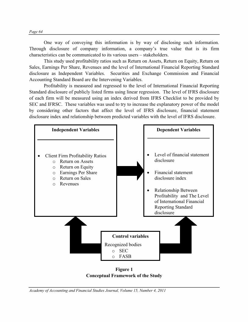
Page 64
Academy of Accounting and Financial Studies Journal, Volume 15, Number 4, 2011
One way of conveying this information is by way of disclosing such information. Through disclosure of company information, a company’s true value that is its firm characteristics can be communicated to its various users – stakeholders. This study used profitability ratios such as Return on Assets, Return on Equity, Return on Sales, Earnings Per Share, Revenues and the level of International Financial Reporting Standard disclosure as Independent Variables. Securities and Exchange Commission and Financial Accounting Standard Board are the Intervening Variables. Profitability is measured and regressed to the level of International Financial Reporting Standard disclosure of publicly listed firms using linear regression. The level of IFRS disclosure of each firm will be measured using an index derived from IFRS Checklist to be provided by SEC and IFRSC. These variables was used to try to increase the explanatory power of the model by considering other factors that affect the level of IFRS disclosure, financial statement disclosure index and relationship between predicted variables with the level of IFRS disclosure.
Figure 1 Conceptual Framework of the Study
Control variables
Recognized bodies o SEC o FASB
Independent Variables
• Client Firm Profitability Ratios
o Return on Assets o Return on Equity o Earnings Per Share o Return on Sales o Revenues
Dependent Variables _______________________
• Level of financial statement
disclosure • Financial statement
disclosure index • Relationship Between
Profitability and The Level of International Financial Reporting Standard disclosure

Page 65
Academy of Accounting and Financial Studies Journal, Volume 15, Number 4, 2011
STATEMENT OF THE PROBLEM The main purpose of this study is to identify the magnitude of financial disclosures by Philippine companies and aims to develop strategy in assuring maximum compliance with International Financial Reporting Standard. This paper also seeks to know the relationship of profitability measures that might affect such IFRS disclosure requirements. Through the aforementioned objectives this study attempts to answer the following questions:
1. What is the extent of compliance of publicly listed corporations in the Philippines, using IFRS disclosure checklist as indicated by the disclosure index?
2. Is there a significant relationship between profitability and the extent of IFRS disclosure index?
SIGNIFICANCE OF THE STUDY
This study has an earnest desire to have a deeper and clearer understanding regarding the extent of International Financial Reporting disclosure of selected publicly listed corporations in the Philippines and aims to develop strategy to which maximum compliance with International Financial Reporting Standard. This study also seeks to identify the relationships between profitability and the level of compliance among publicly listed corporations in the Philippines for the year 2008. The different sectors that may benefit from such are the Accounting Standards Council, PICPA, SEC, Academe, management and the Auditing Firms. The results of this study will be highly beneficial to different members of the business community due to the fact that this study gives them updates on the compliance of different companies that belong to publicly listed corporations in the Philippines on the new standard relating to presentation and preparation of financial statement. International Accounting Standard Board It behooves the IASB to have a better understanding of the result of this study for they can easily determine the loopholes and weaknesses of pronouncements involving the presentation of Financial Statements. The IASB will also find this meaningful because it will give them thought on which among the accounts on the face of the financial statements are not usually given emphasis when it comes to financial reporting. The generated results will provide this sector a basis for suggestions for different companies to comply with the disclosure requirements by the standard and would give them idea regarding factors affecting the company’s level of compliance with international financial reporting standard.

Page 66
Academy of Accounting and Financial Studies Journal, Volume 15, Number 4, 2011
Philippine Institute of Certified Public Accountants The PICPA, with its various arms, needs to be in the know with respect to the study in order to inform its nationwide membership the need for unified reporting system in the midst of diversification. The Security and Exchange Commission, since it is the governing arm with aspect of compliance may set up additional requirements to be followed for the regular submission of Financial Statement Reports and for them to have glimpsed how these companies prepared and presented the financial statement. Academe The Academe’s knowledge on this sector would be of vital importance. As the adage goes, learning is better achieved if you start from the bud. The knowledge imparted to the students would help them be aware of the proper presentation for Financial Statements especially at a time the moment they become professionals and they could share the idea of which factor greatly affect the extent of financial statement disclosure. This will also minimize the curb if not totally eradicate of differing reports. Auditing Firms The Auditing firms, among the entities mentioned, have the greater level of influence in terms of compliance audit. They can recommend the appropriate forms or even inform the clienteles in order to arrive at a more uniform aspect of presentation. The significance of the compliance analysis on the Investors provides an impetus for them to make a faster comparison of the industry performance. The differing Account Titles and presentation serves as an impediment in the typical ratio analysis for such. They can suggest to different financial statement users as to how to focus with different variables affecting the compliance report of the company. Management This study would also be of great help to the management of publicly listed corporations in the Philippines. The management would identify strategy in assuring maximum compliance with International Financial Reporting Standard. They would also know which among profitability ratios that might affect such financial disclosures.

Page 67
Academy of Accounting and Financial Studies Journal, Volume 15, Number 4, 2011
Future researcher The future researchers will likewise benefit from the study. They could make use of the data gathered as baseline information for further researches by considering other industries and other ratios not used in this study and to delve to other industry than Food, Beverage & Tobacco, Telecommunication, and Information Technology Industries.
OBJECTIVE AND METHODOLOGY OF THE STUDY This paper aims (1) to empirically identify the magnitude of financial disclosures by Philippine companies in three selected Industries namely Food, Beverage & Tobacco, Telecommunication, and Information Technology Industries, (2) to investigate whether Philippine publicly listed corporations comply with International Financial Reporting Standard, (3) to develop strategy to aid in maximum compliance with IFRS and (4) to study the relationship of profitability ratios with the level of compliance with IFRS among publicly listed corporations in the Philippines for the year 2008 as this was the most recent year for which annual reports were available at the time of study. To satisfy this objective, the researchers obtained the annual report of publicly listed corporation which serves as secondary data. The researchers quantified the disclosures found in the annual reports by computing the disclosure index. The researchers employed the dichotomous procedure in computing for the disclosure index wherein each company will be awarded a score of ‘1’ if the company appears to have disclosed the concerned disclosure and ‘0’ otherwise. Once scoring of the companies is completed, each company is represented with a score reflecting the number of disclosures against which it was found to have disclosed. After which, the score of the respective company is divided by the total number of score. Consistent with the disclosure index by Cooke (1989, as cited by Hossain et. al., 2006), the disclosure index is computed as follows:
1
jm
j ii
T d=
= ∑
Where: d = 1 if the item di is disclosed; and 0 if the item di is not disclosed. mj = denotes the disclosure item specified in the checklist
jj
j
TDIn
=
Where: Tj = amount computed using Equation 1 nj = number of items expected to be disclosed
Considering the mathematical model for the disclosure index, it is inferred that as the value of the index approaches to 1, the level of disclosure and compliance is higher (the entity
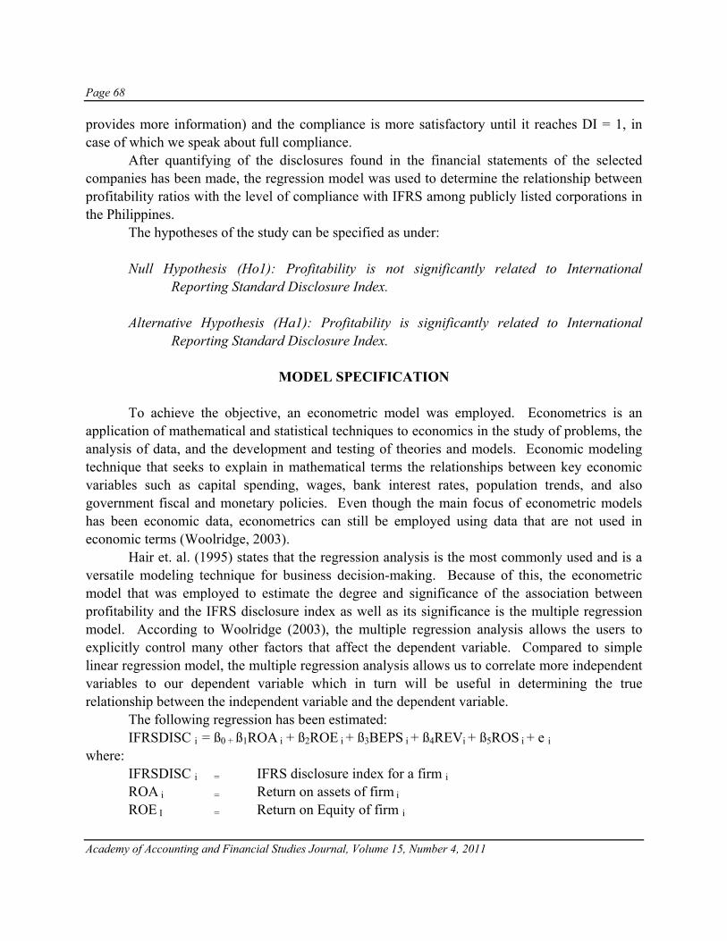
Page 68
Academy of Accounting and Financial Studies Journal, Volume 15, Number 4, 2011
provides more information) and the compliance is more satisfactory until it reaches DI = 1, in case of which we speak about full compliance. After quantifying of the disclosures found in the financial statements of the selected companies has been made, the regression model was used to determine the relationship between profitability ratios with the level of compliance with IFRS among publicly listed corporations in the Philippines.
The hypotheses of the study can be specified as under:
Null Hypothesis (Ho1): Profitability is not significantly related to International Reporting Standard Disclosure Index.
Alternative Hypothesis (Ha1): Profitability is significantly related to International
Reporting Standard Disclosure Index.
MODEL SPECIFICATION To achieve the objective, an econometric model was employed. Econometrics is an application of mathematical and statistical techniques to economics in the study of problems, the analysis of data, and the development and testing of theories and models. Economic modeling technique that seeks to explain in mathematical terms the relationships between key economic variables such as capital spending, wages, bank interest rates, population trends, and also government fiscal and monetary policies. Even though the main focus of econometric models has been economic data, econometrics can still be employed using data that are not used in economic terms (Woolridge, 2003). Hair et. al. (1995) states that the regression analysis is the most commonly used and is a versatile modeling technique for business decision-making. Because of this, the econometric model that was employed to estimate the degree and significance of the association between profitability and the IFRS disclosure index as well as its significance is the multiple regression model. According to Woolridge (2003), the multiple regression analysis allows the users to explicitly control many other factors that affect the dependent variable. Compared to simple linear regression model, the multiple regression analysis allows us to correlate more independent variables to our dependent variable which in turn will be useful in determining the true relationship between the independent variable and the dependent variable. The following regression has been estimated: IFRSDISC i = ß0 + ß1ROA i + ß2ROE i + ß3BEPS i + ß4REVi + ß5ROS i + e i where: IFRSDISC i = IFRS disclosure index for a firm i ROA i = Return on assets of firm i ROE I = Return on Equity of firm i

Page 69
Academy of Accounting and Financial Studies Journal, Volume 15, Number 4, 2011
BEPS i = Basic earnings per share of firm i REV i = Log of the revenues of firm i ROS i = Return on sales of firm i ß0 i ß1 i ß2 i ß3 i ß4 i ß5i = Percentage ownership of shareholders in firm i e 1 = Error term
DEPENDENT VARIABLE In this research, the International Financial Reporting Standards Disclosure Index (IFRSDISCi) is used as the dependent variable. It is aimed to determine how the IFRS compliance as measured by the disclosure index is explained by the independent variables of the regression model as discussed below.
INDEPENDENT VARIABLES The independent variables used in this research are the various profitability measures of the firm. These variables were utilized to determine if the profitability of the firm explains the level of IFRS compliance of the publicly listed corporations in the Philippines. Specifically, the independent variables were computed as follows: ROA: Return on assets is obtained by dividing the net income over total assets. ROA is used since it one of the most common measures of profitability (Hillton, 2007) and it is easy to employ (Hirschey & Wichern, 1984). For this study we expect to have a significant relationship between ROA and IFRS disclosure index. ROE: Return on Equity is computed by net income over total equities. ROE as a measure of company’s profitability may affect the IFRS disclosure. If the company is doing well and earning exceptionally, it must be easier for that company to take necessary measures to comply with the IFRS disclosure requirements. Ergo, it is expected to have a significant relationship between ROE and IFRS disclosure index. BEPS: A basic earnings per share is calculated by dividing net income over weighted average of ordinary shares. We expect that to have a significant relationship between BEPS and IFRS disclosure index. REV: Natural logarithm of sales revenue has also been considered in measuring the profitability of the company. For this study we expect to have significant relationship between log of revenues and IFRS disclosure index. ROS: Return on sales is computed by dividing net income over total sales. Hence, we expect to have significant relationship between ROS and IFRS disclosure index.

Page 70
Academy of Accounting and Financial Studies Journal, Volume 15, Number 4, 2011
RESULTS AND ANALYSIS This portion of the study answers the research problem and objectives of the paper. This chapter presents the summary statistics of the data gathered, the result of the regression analyses made using the IFRS disclosure index as the dependent variable and various profitability measures of the firm as the independent variable.
EMPIRICAL FINDINGS The researchers examined the latest annual reports of different publicly listed corporations that belong to three (3) industries namely Food, Beverage & Tobacco (FBT), Telecommunication (TI) and Information Technology Industries (IT). Disclosure scoring was performed on 981 items of IFRS disclosure checklist 2008 issued by PricewaterhouseCoopers. Section A of the disclosure checklist particularly subsections A1 to A9 was used and considered in this research. Section A includes disclosure for consideration by all entities and has sub-sections such as A1 for General Disclosure, A2 for accounting policies, A3 for Income Statement (and related notes), A4 for Statement of changes in shareholders’ equity (and related notes), A5 for Balance sheet (and related notes), A6 for Cash flow statement, A7 for Business combination and disposal, A8 for Financial instruments and A9 Non-current assets held for sale and discontinued operations. Findings reveal that there are six (6) PLCs comprised the Telecommunication Industry; seven (7) PLCs comprised the Information Technology Industry and twenty one (21) PLCs comprised the Food Beverages and Tobacco. It also depicts the disclosure Index of each of the PLCs, TI garnered a DI of .9886 or 98.86%; IT obtained the maximum level of disclosure was demonstrated scoring a DI of .9900 or 99.00% of the applicable items; and FBT attained a DI of .9894 or 98.94%. This average disclosure level is very satisfactory given the fact that IFRS revisions and new pronouncements on disclosure requirements.
DESCRIPTIVE STATISTICS OF THE DISCLOSURE INDEX As a preliminary tool for data analysis, the researchers computed for the descriptive statistics of the data gathered. Specifically, the researchers considered the mean of the dependent and independent variable as well as its standard deviation. As presented in Table 1, it can be seen that the mean of the disclosure index is .9893 which connotes a high level of compliance with IFRS of the sample firms. Also, it is depicted from the descriptive statistics that the mean of the disclosure index is not far from the minimum and maximum score recorded in the study which means that the level of compliance among the each of the firms in the three industries selected are not far from each other. This observation is confirmed by the computation of the standard deviation, a measure of spread in the sample data. The low disclosure index standard
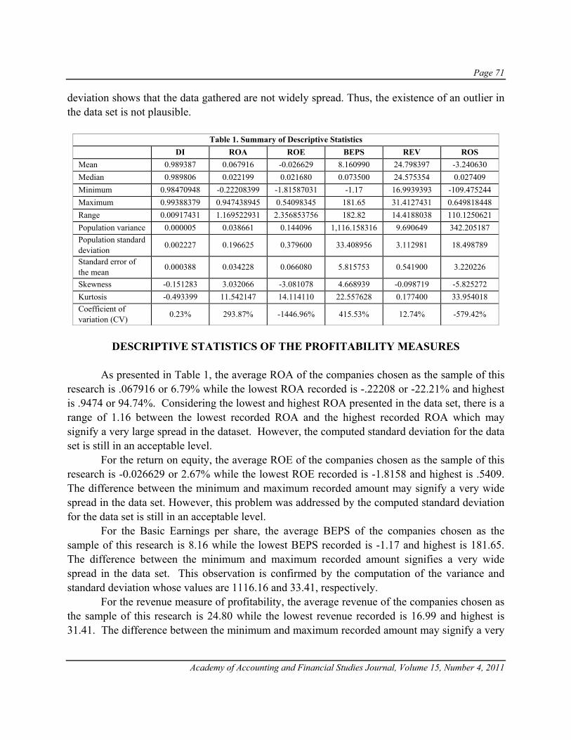
Page 71
Academy of Accounting and Financial Studies Journal, Volume 15, Number 4, 2011
deviation shows that the data gathered are not widely spread. Thus, the existence of an outlier in the data set is not plausible.
Table 1. Summary of Descriptive Statistics DI ROA ROE BEPS REV ROS Mean 0.989387 0.067916 -0.026629 8.160990 24.798397 -3.240630 Median 0.989806 0.022199 0.021680 0.073500 24.575354 0.027409 Minimum 0.98470948 -0.22208399 -1.81587031 -1.17 16.9939393 -109.475244 Maximum 0.99388379 0.947438945 0.54098345 181.65 31.4127431 0.649818448 Range 0.00917431 1.169522931 2.356853756 182.82 14.4188038 110.1250621 Population variance 0.000005 0.038661 0.144096 1,116.158316 9.690649 342.205187 Population standard deviation 0.002227 0.196625 0.379600 33.408956 3.112981 18.498789
Standard error of the mean 0.000388 0.034228 0.066080 5.815753 0.541900 3.220226
Skewness -0.151283 3.032066 -3.081078 4.668939 -0.098719 -5.825272 Kurtosis -0.493399 11.542147 14.114110 22.557628 0.177400 33.954018 Coefficient of variation (CV) 0.23% 293.87% -1446.96% 415.53% 12.74% -579.42%
DESCRIPTIVE STATISTICS OF THE PROFITABILITY MEASURES
As presented in Table 1, the average ROA of the companies chosen as the sample of this research is .067916 or 6.79% while the lowest ROA recorded is -.22208 or -22.21% and highest is .9474 or 94.74%. Considering the lowest and highest ROA presented in the data set, there is a range of 1.16 between the lowest recorded ROA and the highest recorded ROA which may signify a very large spread in the dataset. However, the computed standard deviation for the data set is still in an acceptable level. For the return on equity, the average ROE of the companies chosen as the sample of this research is -0.026629 or 2.67% while the lowest ROE recorded is -1.8158 and highest is .5409. The difference between the minimum and maximum recorded amount may signify a very wide spread in the data set. However, this problem was addressed by the computed standard deviation for the data set is still in an acceptable level. For the Basic Earnings per share, the average BEPS of the companies chosen as the sample of this research is 8.16 while the lowest BEPS recorded is -1.17 and highest is 181.65. The difference between the minimum and maximum recorded amount signifies a very wide spread in the data set. This observation is confirmed by the computation of the variance and standard deviation whose values are 1116.16 and 33.41, respectively. For the revenue measure of profitability, the average revenue of the companies chosen as the sample of this research is 24.80 while the lowest revenue recorded is 16.99 and highest is 31.41. The difference between the minimum and maximum recorded amount may signify a very
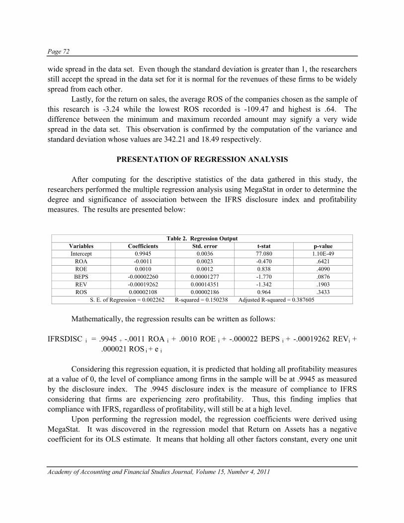
Page 72
Academy of Accounting and Financial Studies Journal, Volume 15, Number 4, 2011
wide spread in the data set. Even though the standard deviation is greater than 1, the researchers still accept the spread in the data set for it is normal for the revenues of these firms to be widely spread from each other. Lastly, for the return on sales, the average ROS of the companies chosen as the sample of this research is -3.24 while the lowest ROS recorded is -109.47 and highest is .64. The difference between the minimum and maximum recorded amount may signify a very wide spread in the data set. This observation is confirmed by the computation of the variance and standard deviation whose values are 342.21 and 18.49 respectively.
PRESENTATION OF REGRESSION ANALYSIS After computing for the descriptive statistics of the data gathered in this study, the researchers performed the multiple regression analysis using MegaStat in order to determine the degree and significance of association between the IFRS disclosure index and profitability measures. The results are presented below:
Table 2. Regression Output Variables Coefficients Std. error t-stat p-value Intercept 0.9945 0.0036 77.080 1.10E-49
ROA -0.0011 0.0023 -0.470 .6421 ROE 0.0010 0.0012 0.838 .4090 BEPS -0.00002260 0.00001277 -1.770 .0876 REV -0.00019262 0.00014351 -1.342 .1903 ROS 0.00002108 0.00002186 0.964 .3433
S. E. of Regression = 0.002262 R-squared = 0.150238 Adjusted R-squared = 0.387605 Mathematically, the regression results can be written as follows: IFRSDISC i = .9945 + -.0011 ROA i + .0010 ROE i + -.000022 BEPS i + -.00019262 REVi +
.000021 ROS i + e i Considering this regression equation, it is predicted that holding all profitability measures at a value of 0, the level of compliance among firms in the sample will be at .9945 as measured by the disclosure index. The .9945 disclosure index is the measure of compliance to IFRS considering that firms are experiencing zero profitability. Thus, this finding implies that compliance with IFRS, regardless of profitability, will still be at a high level. Upon performing the regression model, the regression coefficients were derived using MegaStat. It was discovered in the regression model that Return on Assets has a negative coefficient for its OLS estimate. It means that holding all other factors constant, every one unit
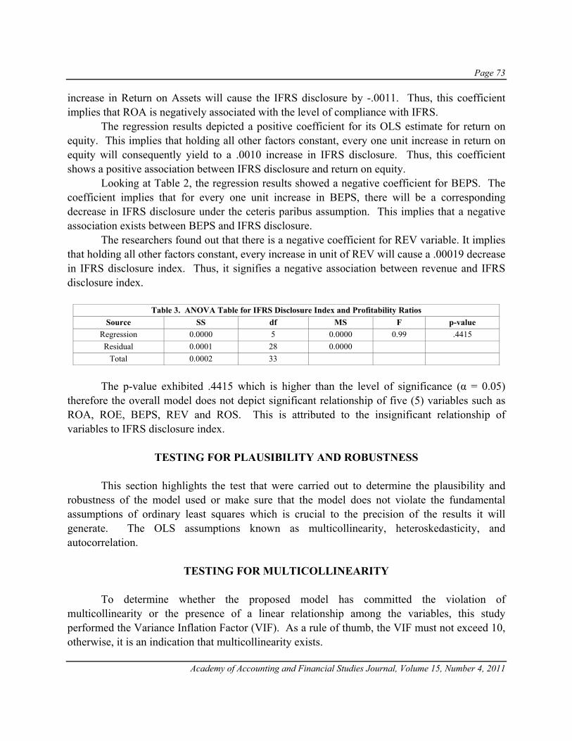
Page 73
Academy of Accounting and Financial Studies Journal, Volume 15, Number 4, 2011
increase in Return on Assets will cause the IFRS disclosure by -.0011. Thus, this coefficient implies that ROA is negatively associated with the level of compliance with IFRS. The regression results depicted a positive coefficient for its OLS estimate for return on equity. This implies that holding all other factors constant, every one unit increase in return on equity will consequently yield to a .0010 increase in IFRS disclosure. Thus, this coefficient shows a positive association between IFRS disclosure and return on equity. Looking at Table 2, the regression results showed a negative coefficient for BEPS. The coefficient implies that for every one unit increase in BEPS, there will be a corresponding decrease in IFRS disclosure under the ceteris paribus assumption. This implies that a negative association exists between BEPS and IFRS disclosure. The researchers found out that there is a negative coefficient for REV variable. It implies that holding all other factors constant, every increase in unit of REV will cause a .00019 decrease in IFRS disclosure index. Thus, it signifies a negative association between revenue and IFRS disclosure index.
Table 3. ANOVA Table for IFRS Disclosure Index and Profitability Ratios Source SS df MS F p-value
Regression 0.0000 5 0.0000 0.99 .4415 Residual 0.0001 28 0.0000
Total 0.0002 33
The p-value exhibited .4415 which is higher than the level of significance (α = 0.05) therefore the overall model does not depict significant relationship of five (5) variables such as ROA, ROE, BEPS, REV and ROS. This is attributed to the insignificant relationship of variables to IFRS disclosure index.
TESTING FOR PLAUSIBILITY AND ROBUSTNESS This section highlights the test that were carried out to determine the plausibility and robustness of the model used or make sure that the model does not violate the fundamental assumptions of ordinary least squares which is crucial to the precision of the results it will generate. The OLS assumptions known as multicollinearity, heteroskedasticity, and autocorrelation.
TESTING FOR MULTICOLLINEARITY To determine whether the proposed model has committed the violation of multicollinearity or the presence of a linear relationship among the variables, this study performed the Variance Inflation Factor (VIF). As a rule of thumb, the VIF must not exceed 10, otherwise, it is an indication that multicollinearity exists.

Page 74
Academy of Accounting and Financial Studies Journal, Volume 15, Number 4, 2011
Table 4. Regression Output Variables Coefficients Std. Error t-stat p-value VIF Intercept 0.9945 0.0036 277.080 1.10E-49
ROA -0.0011 0.0023 -0.470 .6421 1.363 ROE 0.0010 0.0012 0.838 .4090 1.278 BEPS -0.00002260 0.00001277 -1.770 .0876 1.209 REV -0.00019262 0.00014351 -1.342 .1903 1.326 ROS 0.00002108 0.00002186 0.964 .3433 1.087
1.253 Mean VIF
The VIF as computed by Megastat and presented in Table 4, shows that the variables are not highly correlated to each other to warrant any changes in the model. The mean VIF of 1.253 is considerably far from the usual threshold of 10 and even from 5 which some statisticians would use as their decision rule. Thus, this model is relieved from committing the violation of multicollinearity.
Although the variables would seem correlated to each other, there was no presence of multicollinearity found. To validate the premise, this study performed another test for multicollinearity by determining the values of the R-squared and the tolerance values of each variable based on the individual/ auxiliary regression with IFRS disclosure index. Table 5 summarizes that ROE has the lowest R-squared value of .000965 while BEPS has the highest R-squared value of .050231. Consistent with the Lawrence Klien’s rule of thumb, if the R-squared of the auxiliary regressions are greater than the R-squared of the overall regression, then the evidence of multicollinearity is presumed to exist. In this study the overall R-squared is 0.150238 as shown in Table 5, then the variables are not collinearly related. Moreover, a tolerance close to 1 means there is little multicollinearity whereas a value close to 0 suggests that multicollinearity may be a threat. The tolerance values computed by MEGASTAT indicate that values are very close to 1, confirming that no violation was made. As noted, ROE has the highest tolerance value of almost 1.000 while BEPS has the lowest, yet still a very high tolerance value of 0.949769. This shows that the chances of multicollinear relationship are very remote with a high degree of tolerance exists.
Table 5. Summary of R-Squared and Tolerance Values for Auxiliary Regression of Variables Variable R-squared Tolerance *
ROA 0.010190 0.989810 ROE 0.000965 0.999035 BEPS 0.050231 0.949769 REV 0.019979 0.980021 ROS 0.014964 0.985036
Note. * Tolerance = 1 – R-squared

Page 75
Academy of Accounting and Financial Studies Journal, Volume 15, Number 4, 2011
TESTING FOR HETEROSKEDASTICITY To test the presence or absence of any violation that the model might have committed, the model underwent the White’s Test, using the EVIEWS software, for Heteroskedasticity which means that the error of each observation must come form the same probability distribution (Halcoussis, 2005). One way of proving the non-existence of heteroskedasticity was by comparing the p-values and the level of significance (α). If the p-value is greater than α, then the probability of incorrect rejection of the null hypothesis of no heteroskedasticity is greater than its level of significance; then indicating the absence of non-constant variation in the residual terms. Tests exhibited that the p-values is .67450 as shown on Appendix B which is greater than α = 0.05. Thus, IFRS disclosure index model has no heteroskedasticity relationship in this study.
TESTING FOR AUTOCORRELATION The Durbin–Watson statistics is a test statistic used to detect the presence of autocorrelation in the residuals from a regression analysis. It is named after James Durbin and Geoffrey Watson. Autocorrelation is commonly seen or is endemic in time-series analysis or the presence of spatial correlation across the order of observations in a cross-sectional econometric model, it is still important to establish that autocorrelation is not present in the model to enhance the integrity of the conclusion drawn from it. This study used the Run’s test to verify the true state of autocorrelation in the IFRS index model. Using the MEGASTAT software, the expected value of residuals [E ( resid)] and the variance of residuals (σr
2) is computed as
1 22( ) 1T TE residT
= +
22 1 2 12
2 (2 )( 1)r
TT TT TT T
σ −=
−
where: 1T = number of positive residuals
2T = number of negative residuals T = number of observations; and 2
rσ = variance of residuals. Incidentally, rσ refers to the standard deviation of residuals computed as the square root of the variance.

Page 76
Academy of Accounting and Financial Studies Journal, Volume 15, Number 4, 2011
Substituting the formula, this method obtained the figures as presented on Table 6 that will be needed for the Run’s test.
Table 6. Summary Values for the Run’s Test
Item Designation Value
1T Number of positive residuals 15
2T Number of negative residuals 19
T Number of observations 34
( )E resid Expected value of residuals 17.764706 2
rσ Variance of residuals 8.0088078
rσ Standard deviation of residuals 2.8299837
Upon substitution, a confidence interval at 5% level of significance was generated under the following estimation:
E95%CI (Residuals) = E(resid) ± 1.96 (σr) The lower limit was determined to be 12.217938 runs, while the upper limit is 23.311474 runs. Under the Run’s test, the number of changes in the sign of residuals should fall within the confidence interval, or there might be a possibility of spatial correlation in the model. Because this study identified 13 runs that fall within the confidence interval, the IFRS disclosure index model is said to be relieved from committing such violation.
IMPLICATIONS OF THE FINDINGS This study is concerned with the firm’s profitability as an explanatory variable to the level of compliance of the sample firms to IFRS. As the regression results showed, the researchers found out that there is an insignificant relationship between profitability measures and the level of IFRS compliance among the sample firms, thus rejecting the alternative hypothesis presented in this paper. The result of the study was interesting for it shows that profitability does not explain the level of compliance to IFRS of the sample firms selected in this study. It implies that the level of compliance to IFRS will not differ even if the firms have different profitability. According to the study of Valahi and Iatridis (2007), different financial measures such as leverage, profitability, liquidity and growth has an effect on the decision of firms to voluntarily adopt to new accounting policies and pronouncements. Based on this study, the results of this study presenting insignificant relationship showed evidence to the contrary. However, the findings of Valahi and Iatridis (2007) are not unqualified. It was mentioned in

Page 77
Academy of Accounting and Financial Studies Journal, Volume 15, Number 4, 2011
their study that firm’s compliance with accounting regulation is determined by the different financial measures in a manner described as follows:
“Firms may voluntarily abide by an accounting regulation in order to influence their financial performance and suit their corporate plans. For example, following that IAS 1 enhances the quality of financial reporting, firms with higher leverage might be inclined to voluntarily adopt IAS 1 in order to favourably affect their financial position. Voluntary IAS 1 disclosers are generally firms that perform well and particularly tend to exhibit higher profitability and growth. Voluntary IAS 1 disclosers are also firms that tend to provide voluntary accounting disclosures about their financial performance and display high managers’ remuneration and stock returns. Also, firms that raise equity capital appear to voluntarily adopt IAS 1. The study also indicates that large firms, which are more visible in the stock market, voluntarily abide by the reporting requirements of IAS 1 in order to provide evidence of quality in their reported financial numbers and positively influence investors” (Valahi et. al, 2007).
Considering these statements, the relationship between IFRS compliance and profitability measures is dependent on the information that firms wanted to portray using their financial reports. Firms comply with IFRS in order to affect the profitability presented in their financial reports. However, this relationship is subject to a further qualification such that:
“In an efficient stock market, the presentation of low quality accounting information would be expected to be penalised, while quality accounting disclosures would be expected to be rewarded by the stock market (Chung et al., 2002). In an inefficient stock market, investors may misvalue the information content of accounting disclosures, which would in turn lead them to incorrect predictions and decisions (Botosan, 1997). Given that the quality of accounting information is essential for enhancing the stock market efficiency, the questions that arise are how accounting regulation should be improved to encompass all possible areas of accounting practice, and how flexible financial reporting should be.”
It is mentioned as well in the same study, that the relationship between compliance with an accounting regulation is dependent upon the improvement of the efficiency of the stock market. Disclosures made by firms will have possible impact if the stock market is efficient for most of the users understand the meaning of the disclosures that will consequently affect the decision of the managers to have complied fully with IFRS. In this regard, the researchers considered the relationship might as well be read inversely such that profitability of the firms as driven by the users do not primarily drive management’s decision to comply fully with IFRS. This finding is still plausible that it warrants that the Philippine stock market shall further improve its efficiency in order to realize the benefits of the firm’s compliance with IFRS.
CONCLUSIONS All of the relationships deduced from the regression analysis falls below the significance check of (α < 0.05) such that the researchers decided to reject the alternative hypothesis that

Page 78
Academy of Accounting and Financial Studies Journal, Volume 15, Number 4, 2011
there is significant relationship between profitability ratios and IFRS disclosure index; accept the null hypothesis that there is no significant relationship between profitability ratios and the IFRS disclosure index. Ergo, Seen in the Philippine context, profitability measures such as return on assets, return on equity, return on sales, basic earnings per share and revenues have no significant relationship with International Financial Reporting Standard Disclosure Requirements. Applying agency theory in relationship to the correlation between profitability measures and IFRS disclosure index, profitable publicly listed corporations should be disclosing more financial information as their agents or managers want to show off the firm’s good financial performance and financial position. However, the results show also that less profitable publicly listed corporations disclosing more financial information too. This implies how management would be willing to unveil any quantitative and qualitative financial information shown on the face of the financial statements and in its notes to financial statements irrespective the result of operation. The deviation of the results from prior literature was also due to the difference in market conditions and practices here in the Philippines compared to developed countries. Most literature that expressed a positive relationship between profitability and corporate governance disclosures are conducted in developed countries. Several researches suggested that there was a huge difference between developing and developed countries because their model of corporate governance varies in terms of structural characteristics (Rabelo & Vasconcelos, 2002 as cited by Chua et. al., 2009). Taking this into account, Kusumawati (2006) as cited by Chua et. al. (2009) study on Indonesian firms found that profitability affects corporate governance disclosure level negatively. The similarity of the results in Philippine and Indonesian companies is because both countries are located within the same region that have a relatively the same economic conditions and practices. Furthermore, the aforementioned studies from neighboring countries such as Indonesia and Malaysia have relatively comparable results. The Philippines, being a member of the Association of South East Asian Nations (ASEAN) together with Indonesia and Malaysia suggests the resemblance of their operating conditions. The counterintuitive relationship may be credited to the lack of sophistication of the markets within the region on contrast with other developed countries.
RECOMMENDATIONS Audit is as dynamic as the changing landscape of business. With the ever-growing diversification, audit has continued to adapt itself to become attuned with the needs of each sector. Therefore, the continued exchange of knowledge and check-and-balance in compliance audits will be beneficial to the entities mentioned and the end users as well.

Page 79
Academy of Accounting and Financial Studies Journal, Volume 15, Number 4, 2011
The results of this study would provide investors with a more efficient way analyzing the figures presented in the financial statements. The ASC may recommend revisions or even provide a new standard with respect to reporting standards that would cater to the needs of business entities. The PICPA, through its circular and regular seminars, can update its members and serve to upgrade the profession. The SEC may impose stricter guidelines and reject statements haphazardly made or which are not in accordance with the standards. The academe should continue to prepare students and make them more aware of the standards and help the students understand the impact of profitability measures with IFRS disclosure requirements index, while the auditing firms, through their annual audits, should prepare the business sector in the objective of a unified system of preparing and presenting financial statements.
The results of this study are subject to several limitations. The study focuses solely on the relationship between the IFRS disclosure index and profitability measures. The effects of IFRS disclosures on financial performance of the firm value can be studied further. Another limitation is the number of years covered by the study. Increasing the number of years studied can neutralize the effects of irregular events on the data collected and results. It would enable the researchers to measure the performance of the firm on years without significant external factors affecting the economy and the operations of the business. A topic that can be further explored is the relationship between IFRS disclosure index and other financial ratios. Lastly, the population of the research only included firms listed in the Philippine Stock Exchange that belong to Food, Beverage & Tobacco (FBT), Telecommunication (TI) and Information Technology Industries. This population can be broadened by using other Industries with the Securities and Exchange Commission of the Philippines.
REFERENCES Banderlipe, M. C. (2008). The Impact of Selected Corporate Governance Variables in Mitigating Earnings
Management in the Philippines. Botosan, C. A. (1997). Disclosure Level and The Cost of Equity Capital. Accounting review, 72(3), 323–349. Botosan, C. A. (1997). Disclosure level and the cost of equity capital. Acc. Rev. 72, 323–349. Cataldo, A. (2003). Agency theory and principal-agent problems. In A. Cataldo (Ed.) Information asymmetry: A
unifying concept for financial and managerial accounting theories. Oxford, United Kingdom: Elsevier. Chiang, H. (2005). An empirical study of corporate governance and corporate performance. The Journal of
American Academy of Business, 6, 95-101. Chua, et. al. (2009). The Relationship Between Profitability and Selected Structure-Related Variables with the Level
of Corporate Governance Disclosures among Publicly-Listed Companies in the Philippines. Unpublished Undergraduate Thesis: De La Salle University, Manila, Philippines.
Chung, R., M. Firth & J. Kim (2002). Institutional monitoring and opportunistic earnings management. J. Corp. Finance 8 (1), 29–48.

Page 80
Academy of Accounting and Financial Studies Journal, Volume 15, Number 4, 2011
Cooke, T. E. (1989). Voluntary corporate disclosure by Swedish companies. Journal of international financial management and accounting, 1, 171-195.
Hair, J. F., R. E. Anderson, R. Tatham & W. C. Black (1995). Multivariate Data Analysis. Englewood Cliffs, New Jersey: Prentice Hall.
Halcoussis, D. (2005). Understanding Econometrics. Mason, Oh: Thomson/South-Western. Hillton, R. (2007). Managerial Accounting: Creating Value in a Dynamic Organization. New York: McGraw Hill. Hirschey, M, & W. Wichem (1984, Oct.). Accounting and market-value measures of profitability: Consistency,
determinants, and uses. Journal of Business & Economic Statistics, 2(4), 375-383. Hossain D. M. & A. R. Khan (2006). Disclosure on Corporate Governance Issues in Bangladesh: A survey of the
Annual Reports. Published in ‘The Bangladesh Accountant’, Quarterly Journal of Institute of Chartered Accountants of Bangladesh, January-March, 2006, pp. 95-99.
Jensen, M. C. (1993). The modern industrial revolution, exit, and the failure of the internal control system. Journal of Finance, 48, 831-880.
Jensen, M.C. and W. H Meckling (1976). Theory of the Firm: Managerial Behaviour, Agency Costs and Ownership Structure, Journal of Financial Economics, Vol. 3, October, pp. 305-360.
Kusumawati, D. N. (2006). Profitability and Corporate Governance Disclosure: An Indonesian Study. Simposium Nasional Akuntansi, 9, 1-12.
Lang, M. H. and R. J. Lundholm (1993). Cross-sectional determinants of analyst ratings of corporate disclosures. Journal of Accounting Research, 31(2), 246-271.
Lee, B. & B. Choi (2002). Company size, auditor type, and earnings management. Journal of Forensic Accounting, 3, 27-50.
Padayogdog, C. (2003). A Study on the Incentives Influencing the Practice of Creative Accounting in Selected Business Establishments in Davao City. Unpublished Master’s Thesis, De La Salle University, Manila, Philippines.
Rabelo, F. & F. Vasconcelos (2002). Corporate Governance in Brazil. Journal of Business Ethics, 37(3), 321-35. Racasa, C. R. (2003). Determinants of the Extent of Disclosure in Financial Statements of Metro Cebu
Corporations Audited by Non-Affiliated CPA. Graduate School of Business. De La Salle - Manila. Richardson, V. (2000). Information asymmetry and earnings management: Some evidence. Review of Quantitative
Finance and Accounting, 15, 325-347. Sabado, Joan P. (2005). The Impact of Firm Characteristics on the Extent of Financial Disclosure in Company
Website of the Top 200 Philippine Corporations. Graduate School of Business. De La Salle - Manila. Spence, M. (1973). Job market signaling. Quarterly Journal of Economics, 87(3), 355-374. Tan, R. (2003). Highly Valued Companies are Good Flirts. Oaktree Research. Retrieved April 26, 2005 from
http://www.oaktree-research.com. Valahib, S. & G. Iatridis (2007). Research in International Business and Finance 24 (2010) 1-14. Voluntary IAS 1
accounting disclosures prior to official IAS adoption: An empirical investigation of UK firms. ScienceDirect. www.elsevier.com/locate/r ibaf.
Valix, Conrado T., et. al. (2009). Financial Accounting. Volume One. Manila, Philippines: GIC Enterprises & Co., Inc.
Watts, R., & J. Zimmerman (1986). Positive Accounting Theory. Englewood Cliffs, NJ: Prentice Hall. Woolridge, J. (2003). Introductory Econometrics. Mason, OH: Thomson/South-Western.

Page 81
Academy of Accounting and Financial Studies Journal, Volume 15, Number 4, 2011
Appendix A: Public Listed Corporations and Its Disclosure Index BY INDUSTRY Disclosure Index (DI) 1 Telecommunication Industry 0.9886 2 Information Technology Industry 0.9900 3 Food, Beverages and Tobacco Industry 0.9894 By Public listed Corporations 1. Telecommunication Industry Disclosure Index 1 TCI A 0.9878 2 TCI B 0.9908 3 TCI C 0.9888 4 TCI D 0.9908 5 TCI E 0.9857 6 TCI F 0.9878 2. Information Technology 1 IT A 0.9888 2 IT B 0.9857 3 IT C 0.9929 4 IT D 0.9898 5 IT E 0.9918 6 IT F 0.9908 7 IT G 0.9898 3. Food Beverages and Tobacco 1 FBT A 0.9888 2 FBT B 0.9918 3 FBT C 0.9857 4 FBT D 0.9918 5 FBT E 0.9898 6 FBT F 0.9847 7 FBT G 0.9888 8 FBT H 0.9918 9 FBT I 0.9908 10 FBT J 0.9898 11 FBT K 0.9878 12 FBT L 0.9867 13 FBT M 0.9939 14 FBT N 0.9908 15 FBT O 0.9888 16 FBT P 0.9867 17 FBT Q 0.9878 18 FBT R 0.9898 19 FBT S 0.9929 20 FBT T 0.9888 21 FBT U 0.9898

Page 82
Academy of Accounting and Financial Studies Journal, Volume 15, Number 4, 2011
Appendix B: White Heteroskedasticity Test: F-statistic 0.809172 Probability 0.674540 Obs*R-squared 18.85442 Probability 0.531306
Test Equation: Dependent Variable: RESID^2
Method: Least Squares Date: 12/08/09 Time: 16:00
Sample: 1 34 Included observations: 34
Variable Coefficient Std. Error t-Statistic Prob. C 0.000242 0.000149 1.619096 0.1294 ROA -0.001749 0.000988 -1.770345 0.1001 ROA^2 -0.000240 0.000112 -2.134529 0.0524 ROA*ROE 0.000318 0.000218 1.460358 0.1679 ROA*BEPS -2.95E-05 6.32E-05 -0.467324 0.6480 ROA*REV 6.60E-05 3.47E-05 1.903323 0.0794 ROA*ROS -0.000385 0.000576 -0.667876 0.5159 ROE 0.000712 0.000385 1.847211 0.0876 ROE^2 -6.93E-06 4.56E-05 -0.152047 0.8815 ROE*BEPS -3.17E-06 4.12E-05 -0.077077 0.9397 ROE*REV -2.76E-05 1.48E-05 -1.861127 0.0855 ROE*ROS 0.000422 0.000561 0.751866 0.4655 BEPS 1.01E-05 1.18E-05 0.856351 0.4073 BEPS^2 -2.12E-08 5.35E-08 -0.395760 0.6987 BEPS*REV -3.34E-07 4.49E-07 -0.744157 0.4700 BEPS*ROS 2.05E-05 3.60E-05 0.567975 0.5797 REV -1.84E-05 1.18E-05 -1.557645 0.1433 REV^2 3.53E-07 2.33E-07 1.515272 0.1536 REV*ROS -4.63E-06 2.93E-06 -1.578363 0.1385 ROS 0.000109 6.98E-05 1.565437 0.1415 ROS^2 -7.80E-07 8.29E-07 -0.941885 0.3634 R-squared 0.554542 Mean dependent var 4.21E-06 Adjusted R-squared -0.130778 S.D. dependent var 4.90E-06 S.E. of regression 5.21E-06 Akaike info criterion -21.21726 Sum squared resid 3.53E-10 Schwarz criterion -20.27451 Log likelihood 381.6934 F-statistic 0.809172 Durbin-Watson stat 2.266353 Prob(F-statistic) 0.674540

Page 83
Academy of Accounting and Financial Studies Journal, Volume 15, Number 4, 2011
FINANCIAL PERFORMANCE OF COMPUTER NETWORK AND INFORMATION TECHNOLOGY
SERVICES COMPANIES IN BULL AND BEAR MARKETS
Anne Macy, West Texas A&M University Neil Terry, West Texas A&M University
Jean Walker, West Texas A&M University
ABSTRACT Stock market volatility has been omnipresent in the information technology sector. This manuscript compares the stock performance of computer network and information technology companies across six different twenty-month periods between the years 1996-2006. The focus periods include the browser era, the Y2K era, the post-Y2K era, the post-9/11 era, the outsourcing era and the mobile/wireless era. The lowest stock market returns are in the post-Y2K and post-9/11 eras for four of the five computer network and information technology services firms in the research cohort. The highest stock market returns for the five computer network and information technology services firms are in four different periods. The firms in the study show a tendency to experience high industry correlation in a bear market but little correlation during a bull market. The results imply that the computer network and information technology services industry has characteristics that are consistent with being a blockbuster instead of a commodity.
INTRODUCTION The information technology sector has transformed the economy and changed the basis of competition (Sampler, 1998). Information technology boosts the efficiency of the decision-making process and is perceived by many executives as an integral part of their business strategy (Molloy and Schwenk, 1995; Bartholomew, 1998). Investors have struggled to comprehend the potential and the limitations of information technology companies as the industry has continued to evolve over time. Not surprisingly, the volatility of stock prices for information technology firms has been extreme as many companies struggle to survive in the next few years after reaching a peak stock valuation. On March 10, 2000 the NASDAQ composite peaked at an intra-day high of 5,132 and declined to half of its value within a year before finding a bear market bottom on October 10, 2002 with an intra-day low of 1,108. The excessive rise and fall

Page 84
Academy of Accounting and Financial Studies Journal, Volume 15, Number 4, 2011
of information technology companies offers a unique opportunity to evaluate industry nuances associated with bear and bull markets. The purpose of this research is to compare the stock market performance of multiple computer network and information technology services companies across six information technology eras. The six period classifications are the browser era, Y2K era, post-Y2K era, post-9/11 era, outsourcing era, and mobile/wireless era. Cisco Systems (CSCO), 3Com (COMS), Ericsson (ERIC), Nortel Networks Corporation (NT), and Yahoo Inc. (YHOO) are the five computer network and information technology services firms included in the study. The organization of this manuscript divided into five sections. The first section offers a discussion on the literature related to the financial performance of information technology companies. The next section offers background information relating to the six information technology eras applied to this study. The third section discusses the computer network and information technology services industry and the five specific companies that are the focus of this study. The fourth section presents data and methodology. The fifth section puts forth results from the application of a nonparametric technique to compare stock market returns across different information technology eras for the six companies. The final section offers concluding comments.
REVIEW OF THE LITERATURE Academic research identifying structural economic changes that influence stock prices mostly focuses on major crashes in the history of financial markets (Higgins & Osler, 1997; Allen & Gale, 2000; Cocca, 2005). Although a relatively new topic for the information technology sector, there are numerous studies in finance theory that focus on the development of speculative bubbles and stock market volatility (Camerer, 1989; Allen & Gale, 2000). Stock market volatility is explained by various approaches, which differ in essence according to assumptions made with regard to market efficiency (Sornette & Malevergne, 2001). Stock market performance of information technology companies reveals the sector has greater volatility than most other economic sectors (Demers & Lev, 2001; Ofek & Richardson, 2003; Kamssu, Reithel, & Ziegelmayer, 2003). Terry, Macy, and Abdullat (2010) find a correlation of stock prices for vertically integrated technology companies in a down market but bull markets are not highly correlated within the vertically integrated firms. Cocca (2005) puts forth one of the few studies exploring potential reasons for the stock market volatility of information technology companies. The study uses a broad media database to analyze the informational and media environment surrounding the market highs for technology stocks and explores potential trigger events that could cause an Internet bubble to burst. Two key informational event triggers are public awareness of the human genome research results and the publication of a study by Barron’s magazine about Internet companies’ burn rates.

Page 85
Academy of Accounting and Financial Studies Journal, Volume 15, Number 4, 2011
Cocca (2005) concludes diffusion data of the informational events show a long-term impact of the Barron’s study on media, financial analyst and consequently investor focus. Researchers are becoming more and more interested in studies relating IT investment and firm performance (Im, Dow, & Grover, 2001). The studies have produced a wide range of performance results that are negative or not conclusive (Tam, 1998), mixed (Avison, Eardley, & Powell, 1998; Ranganathan & Samarah, 2001), or positive a positive and significant relationship between IT investment and firm financial performance (Im, Dow, & Grover, 2001). Kamssu, Reithel, & Ziegelmayer (2003) explore the impact of information technology and stock returns. They conclude that Internet-dependent firms have lower excess returns than non-Internet firms do in a booming economy and that Internet stocks trade at relatively higher prices than non-Internet stocks. The explosion of Internet technology and behavior of investors and decision makers toward firms that use the Internet suggest that Internet technology must have an impact on firms’ market performance. Stock performance helps investors gauge how well their managers are handling their money. Several studies have proposed different methods to assess stock performance. Armitage & Jog (1996), Rogerson, (1997), and Clinton & Chen (1998) have used economic value as a measure of performance. The economic value added is obtained by comparing profits with the cost of capital involved in obtaining these profits (Stephens & Bartunek, 1997). Johnson & Pazderka (1993) and Sundaram, John, and Kose (1996) have employed stock market performance estimates to measure firm performance. Fama & French (1995), Loughran (1997), Zaher (1997) and Ranganathan & Samarah (2001) employ the stock excess returns based on the Capital Asset Pricing Model (CAPM) to measure stock performance. Historically, the stock values of information technology firms bear very little relationship to classical business performance measures (Savitz, 1998), which creates a need for non-traditional proxies and estimation methods. The statistical methodology incorporated in this study employs a nonparametric approach to comparing the stock market performance of firms across a decade of six different development stages for the information technology industry. The study uses multiple years of data based on the diffusion model hypothesis that the spread of information needs time and stock price momentum reflects gradual diffusion of firm-specific information (Hong & Zhu, 2006). There is no research focusing on stock market volatility of computer network and information technology services companies.
TECHNOLOGY ERAS Between 1996 and 2006, several major events in the field of information technology made a lasting impact on many businesses and consumers. Six implicit periods are identified for the purposes of this study. Although somewhat arbitrary, the six periods are placed in twenty-month segments in an effort to capture stock market returns in a broad representative timeframe.

Page 86
Academy of Accounting and Financial Studies Journal, Volume 15, Number 4, 2011
The six period classifications are the browser era, Y2K era, post-Y2K era, post-9/11 era, outsourcing era, and mobile/wireless era. The browser era is defined in the study as the 20-month period of August 1996 through March 1998. The World Wide Web was but a few years old when Mosaic, often considered the first browser, was introduced. The web was massive and complicated. Prior to Mosaic, access to the Internet was largely limited to text, with any graphics displayed in separate windows. Users needed to possess certain technical knowledge and skills to exploit available capabilities and access both the Internet and the web. Mosaic eventually became Netscape. The success of Netscape gained the attention of Microsoft, which developed the Explorer browser. A cluster of related and supporting technologies came together to make the browser a significant innovation breakthrough. The browser era developed with the assistance of computer servers, bandwidth affordability and availability, content providers, and communication links. The browser interface made it easier for users to connect to the web and created a significant critical mass of users (Cocca, 2005). The use of browsers to connect to the Internet pressured software developers and content providers to adhere to certain accepted specifications and standards. These standards and specifications enhanced the interoperability of web-related products and services. For years, enterprises struggled to find reliable, cost-effective ways to integrate and automate critical processes between different application packages. The web-enabled applications and technology provided the enterprises with the ability to integrate different systems and application types regardless of their platform, operating system, programming language or locations. In essence, the browser was the key that unlocked the World Wide Web to a massive number of users. Netscape was the most used browser to access the web. It allowed millions of users to navigate the web and was the vehicle that linked people and information. The catalyst marked the boom in the Internet. The browser made it possible for millions of users to access the web daily, to send messages and to perform business transactions that would not have been possible without the browser. The browser has changed the way society communicates, created new businesses and contributed to the demise of other businesses. The Y2K era in this study is the 20-month period of April 1998 through November 1999. In the early days of software development and hardware design, it was common practice to use standard two-digit shorthand to indicate the year. This practice infiltrated many software applications and hardware designs. In the early nineties, this became known as the Y2K problem. The Y2K problem implied that some software and hardware would not perform as expected after December 31, 1999. While many were relieved that the catastrophic consequence of Y2K did not materialize, it is clear that this era had profound impact on the amount of expenditures in the field of information technology. The commercialization of the Internet and the need to overhaul information technology infrastructure in preparation to address the potential Y2K problem was a significant driving force. The Department of Commerce estimated that there was approximately $100 billion spent to address the Y2K problem in the United States (Manion & Evan, 2000). The significance of Y2K is more than the expenditure amount, it also
Page 87
Academy of Accounting and Financial Studies Journal, Volume 15, Number 4, 2011
provided opportunities to shift to new computing platforms, implementing new approaches to software applications development and highlighting the relevant role of information technology to the overall enterprise’s business strategy. The post-Y2K era in this study is the 20-month period of December 1999 through July 2001. The 2001 year had been a bust with the dot-com implosion and the downturn of the economy. The pre-Y2K buildup resulted in the post-Y2K bust for many information technology companies. Many companies cut back on information technology expenditures during this era because of the significant expenditures in the preceding era. Despite the bursting of the dot-com bubble, significant advances in information technology advances continued during this era. The importance of critical infrastructure, the need for compliance with security regulations, the importance of business continuations plans, and data mining/warehousing were four major themes that emerged during this time (Terry, Macy, & Abdullat, 2010). This study defines the post-9/11 era as the 20-month period of August 2001 through March 2003. The event of September 11 accentuated the importance and the vulnerability of information technology in the event of catastrophic attack. It necessitated the need to develop plans to identify its critical infrastructure that is required to maintain minimum operation of the economy and government. The security of critical infrastructure became a vital concern. Security of critical infrastructure and other resources went through extensive change to mitigate the risks. Federal regulations tightened security regulations to include many aspects of business processes and functions. Information technology was targeted as the means to meet the security concern. The sense of urgency to meet security demands and concerns by the federal government made it easier to fund many of the new research and development activities by businesses. Moreover, many businesses recognized the value of computer security as a large, emerging market. During this time, the importance of data centers’ redundancy of data and the need for diversity of geographic concentration of information technology resources gained in relevance and significance (Terry, Macy, & Abdullat, 2010). In addition, network infrastructure influenced businesses in a very profound manner that required continued increase in computing power. Barriers that existed between firms for most of the 20th century gave way to accommodate the need for partnership-based opportunities afforded through e-business. The need for interoperability and flexibility increased during this era to exploit new business opportunities. This created a demand for new system architectures to mitigate the shortcomings of grid computing and client server technologies. The continuous decline in the storage cost of data, the increase of computing power, and the availability of broadband bandwidth reduced the incentive for firms to discard any data (Hong & Zhu, 2006). The availability of stored digital data and information presented firms and government agencies with a major challenge to identify ways to make some sense of the huge amount of data. The government’s heightened concern with security was instrumental in funding new developments in data mining and contributed to the increased use of business-intelligence software to mine huge amounts of stored data.

Page 88
Academy of Accounting and Financial Studies Journal, Volume 15, Number 4, 2011
The outsourcing era is defined in the study as the 20-month period of April 2003 through November 2004. In this era, companies were looking for different measures to cut costs and to improve the balance sheet. Outsourcing and off shoring became prominent business strategies to reduce operational cost, to enhance services, and to improve financial performance. In addition to the economic and market conditions, three Laws influenced this period: Moore's (growing power of computer chips), Metcalfe's (growing network usefulness) and Gilder's (growing communications bandwidth). These laws transformed processes, products and services (Terry, Macy, & Abdullat, 2010). Combining the economic conditions and the changes in information technology made it possible to reduce cost but to continue performing certain functions of the business at the same or higher level. Businesses quickly realized the cost advantage of developing and maintaining their software applications in India, China and Eastern Europe. In looking back at that era, it is clear that notwithstanding the challenging economic conditions at the time, it marked the beginning of accepting outsourcing as a cost-reduction strategy (Hong & Zhu, 2006). The outsourcing phenomena affected many areas of information technology including software development and programming, technical support, calling centers and customer services. The mobile/wireless era is the 20-month period of December 2004 to August 2006. The term mobile computing is the use of portable computing devices either in transit or from a remote location. Wireless technology had been around for many years, but the industry-transformed society during this era. The mobile computing environment is composed of small devises that permit users to have access to information almost anywhere at any time (Cocca, 2005). The increased access by users to the Internet, the innovation of wireless technology, and the high number of cellular phone services contributed to the growth of mobile computing. Moreover, the dependency and the reliance on laptops and hand-held devises to perform computing functions increased the demand for mobile and wireless products and services.
INDUSTRY OVERVIEW The computer network and information technology service industry is characterized as one that must be extremely nimble and fast at meeting the needs of customers. The firms’ customers in this industry are primarily large businesses both within the technology sector but also in all other sectors. Customers who purchase network equipment seek equipment that will meet their needs for an extended time period but with the capability of being upgraded as needed. High-end network equipment can cost over $100,000, so the purchases are viewed as capital equipment and are highly scrutinized by the buyers. While price does factor into the decision, buyers also recognize that performance and ease of maintenance are other major, important decision factors. For the technology services part of the industry, customers seek products that come with substantial and timely service packages. For the firms, selling the equipment and then the service package extends the value of each sale and provides an
Page 89
Academy of Accounting and Financial Studies Journal, Volume 15, Number 4, 2011
opportunity to solidify the relationship and thus expand it into future sales. Because of the size and technical requirements of the hardware in this industry, it is capital intensive but with a requirement of highly-skilled employees who can explain to the customers how the product can benefit the buyer firm. In order to stay fresh and gain access to new markets, many of the firms are active acquirers of competitors. The goal of the acquisitions is to gain a blockbuster product. Customers and stock investors quickly change allegiance to the latest hit product and reward it with sales and stock price jumps. The five computer network and information technology services companies included in the study are Cisco Systems (CSCO), 3Com (COMS), Ericsson (ERIC), Nortel Networks Corporation (NT), and Yahoo Inc. (YHOO). The five firms in this study all followed an aggressive acquisition strategy to gain access to blockbuster products or customer bases. Cisco Systems (CSCO) is a leading supplier of internetworking hardware, such as routers and switches, to direct data, including voice and video. Approximately half of its revenues are from outside of North America (Value Line, 2010). Like the other firms in the industry, Cisco is an active buyer of competitors and firms in related but new markets. Notable purchases over the years have included Kalpana, a switch manufacturer in 1994, Percept Software, video transmission software maker in 1998, Andiamo Systems, storage network switch maker in 2002, Linksys, home network specialist in 2003 and WebEx Communications, conference systems in 2009 (Hoover’s Online, 2010). The list demonstrates how Cisco uses acquisitions to strategically place itself in all points of the networking supply chain but without having to conduct the initial research & development required of each new sub-area of networking. Cisco’s best period was the Y2K period. Firms in all industries were upgrading systems and seeking better control over their entire information technology structure. Earnings per share during the Y2K era grew at over 35% annually (Value Line, 2010). While slightly slower than during the browser era, investors recognized the central role Cisco played in the technology sector and rewarded it with a P/E ratio well above 100 (Business & Company Resource Center, 2010). During the post-Y2K era, earnings dropped by over 50%, even though revenues increased (Value Line, 2010). The firm had invested heavily in Internet protocol network equipment, whose sales dropped sharply during the technology bust (Mergent Online, 2010). The stock price dropped sharply, matching the decline in earnings. The post-9/11 era was tough for Cisco as it looked to diversity its product line and rebuild cash flow. By 2004 during the outsourcing era, Cisco had rebounded enough to resume its acquisition strategy (Hoover’s Online, 2010). Stock investors responded positively to Cisco’s strategy and increased the P/E ratio to about 30, giving Cisco its second best performing era (Value Line, 2010). Cisco’s upward trend continued during the mobile/wireless era, albeit at slower growth rates. Its P/E ratio fell by 1/3 as its stock price trended upward slightly (Value Line, 2010). Overall, Cisco has learned from its mistakes during the post-Y2K era and maintains an acquisition strategy that does not deplete its cash.
Page 90
Academy of Accounting and Financial Studies Journal, Volume 15, Number 4, 2011
3Com (COMS) is the upstart networking firm in the industry who tries to play with the big players. With a market capitalization that usually ranges from 1% to 3% of Cisco’s market capitalization, 3Com spends as if it is the biggest player in town including naming Candlestick Park in San Francisco 3Com Park from 1995 to 2000 (Value Line, 2010). Robert Metcalfe, the inventor of the Ethernet for Xerox, founded 3Com. Using the Ethernet as its base technology, 3Com developed ancillary hardware products (Hoover’s Database, 2010). Of the five firms in the study, 3Com had the lowest performance in the browser and Y2K eras. Operating costs fluctuated as the firm tried to integrate all of the firms it had acquired (Value Line, 2010). In particular, 3Com purchased U.S. Robotics and the Palm Pilot PDA in 1997. Integrating the larger U.S. Robotics was problematic and resulted in layoffs, inventory problems, negative press, and finally, one of the largest shareholder lawsuits and settlements in history (Hoover’s Online, 2010). During the post-Y2K era, the stock price plummeted from above $100 per share to under $10 per share (Value Line, 2010). In an effort to raise cash, 3Com spun-off Palm in 2000 (Business & Company Research Center, 2010). The post-9/11 era saw 3Com refocus its business away from consumers and to business along with reducing 30% of its workforce (Hoover’s Online, 2010). Investors responded positively to the firm’s actions and rewarded it with an increasing stock price, albeit modestly (Value Line, 2010). This is especially surprising considering that 3Com posted negative earnings from 2001 through 2006. During the outsourcing and mobile/wireless eras, 3Com continued to divest itself of ancillary product lines, which raised cash for the firm (Hoover’s Online, 2010). Additionally, the firm began to move aggressively into Asia, particularly China. Its acquisitions and strategic alliances produced new products and sales (Mergent Online, 2010). China is the source of over half of 3Com’s sales (Value Line, 2010). These actions helped 3Com return to profitability and a positive cash flow by the end of the wireless era. Ericsson (ERIC), one of the largest Swedish companies, is a leading provider of telecommunication and data communication systems and related services covering a range of technologies, including especially mobile networks. Directly and through subsidiaries, it also has a major role in mobile devices and cable TV and IPTV systems (Value Line, 2010). Throughout the 1990s, Ericsson held a 35-40% market share of installed cellular telephone systems (Hoover’s Online, 2010). Like most of the telecommunications industry, Ericsson suffered heavy losses after the telecommunications crash in the early 2000s. It was forced to do a 1-for-10 reverse stock split in 2002 (Value Line, 2010). On October 1, 2001 the handsets division formed a joint venture with Sony called Sony Ericsson. Ericsson is now a major provider of handset cores and an infrastructure supplier for all major wireless technologies (Hoover’s Online, 2010). It has played an important global role in modernizing existing copper lines to offer broadband services and has actively grown a new line of business in the professional services area. Ericsson’s focus on the hardware for networks has allowed it to survive the rough times. Its North American business is less than 10% of total sales while Europe is more than 50% of revenues (Value Line, 2010). Ericsson, while considered a quality

Page 91
Academy of Accounting and Financial Studies Journal, Volume 15, Number 4, 2011
product, has never been able to make a huge dent in North America because its wireless products are functional but without the features of an iPhone or BlackBerry (Business & Company Resource Center, 2010). In contrast, its network hardware has a strong reputation and is the growth engine for the firm. The firm’s net profit margin bounced from negative values in 2001 and 2002 to over 11% by 2004. Its focus on infrastructure hardware is profitable; the net profit margin has been close to or over 15% since 2005 (Mergent Online, 2010). U.S. investors have not recognized fully the strengths of Ericsson’s business. The lack of a consumer presence has resulted in a declining P/E ratio. Ericsson’s P/E ratio was close to 90 in 2000 but less than 20 since 2004 (Value Line, 2010). It is one of the few technology companies to pay a dividend, which increased yearly since the 2005 reinstatement. Over the entire 120-month period, Ericsson has the lowest total return. Nortel Networks (NT/NRTLQ) is a leader in telecommunications networking. Originally, a part of Bell Canada, Nortel was a division in a series of telecommunications firms until its current incarnation created during the browser and Y2K eras (Hoover’s Online, 2010). As one of the first firms to move into the Internet hardware business, Nortel supplemented its product line with an aggressive acquisition strategy acquiring Bay Networks and Shasta Networks (Business & Company Resource Center, 2010). The acquisitions helped Nortel increase its earnings growth rate to above 30% during the browser era. Investors supported the acquisition strategy and increased the P/E ratio by 60% during the Y2K era (Value Line, 2010). However, Nortel’s push into the Internet business ensured that it would suffer when the technology bubble burst. Its earnings per share and cash per share turned negative. Investors punished the stock, whose price fell by 95% during the post-Y2K era (Value Line, 2010). Nortel responded by realigning its business and cutting its workforce. In 2001 alone, it laid off 50,000 employees. It also sold business, sometimes at a loss, to gain cash (Hoover’s Online, 2010). By the end of the post-9/11 era, the firm had returned to positive earnings and cash flow (Value Line, 2010). Nortel was an active member of the outsourcing era. It signed a deal with Singapore’s Flextronics to outsource all of its manufacturing. This allowed Nortel to focus on design and marketing of products but not the quality control issues associated with manufacturing (Hoover’s Online, 2010). Investors responded positively and pushed the stock price above $80 (Value Line, 2010). During the mobile/wireless era, Nortel focused on increasing the speed and capabilities of its network products. In particular, it focused its research and development on 3G and 4G technologies (Mergent Online, 2010). Overall, Nortel has the lowest performance of the five stocks examined. After starting out on a high, Nortel could not recreate the products or the excitement once the Internet became routine and the focus needed to shift to cost-control, which was not a strength of Nortel. Yahoo! Inc. (YHOO) is a leading provider of Internet services including search, auctions, and mail to customers. Unlike the other firms in this study, Yahoo focuses more, but not completely, on services to the retail consumer (Hoover’s Online, 2010). Yahoo went public during the browser era even though it did not have positive earnings until 1998 (Value Line,

Page 92
Academy of Accounting and Financial Studies Journal, Volume 15, Number 4, 2011
2010). Just as the other firms in the industry used acquisitions as a central part of their corporate strategy, Yahoo actively purchased firms with new ideas or existing customers. During the Y2K era, Yahoo looked for firms with products to monetize the Internet such as direct marketing firm Yoyodyne and Internet communications firm Broadcast.com (Hoover’s Online, 2010). During the Y2K era, Yahoo’s dominance of the search engine and ability to help businesses turn a profit on Internet customers was rewarded by stock investors who made it the darling of the Internet boom and increased its P/E ratio to over 500. However, during the technology bust, Yahoo struggled and its stock price fell to lows not seen since just after it went public (Value Line, 2010). The post-Y2K era was a time of restructuring for Yahoo. In 2000, it announced it would charge fees to list items on its auction site. Users responded by abandoning the site (Hoover’s Online, 2010). Yahoo struggled to find a way to make consumers pay for Internet services. Yahoo reduced its workforce by about 1000 employees (Hoover’s Online, 2010). During the post-9/11 era, Yahoo moved into new areas including music and ebooks. It also redesigned its webpages to allow for more advertising (Business and Company Resource Center, 2010). Stock investors responded positively and increased the stock price (Value Line, 2010). During the outsourcing era, Yahoo finally regained its stride. Increasing revenue from online advertising and paid search resulted in a doubling of sales and earnings during this period. Yahoo even had a 2-for-1 stock split in 2004 (Value Line, 2010). By the mobile/wireless era, Yahoo continued to expand its reach internationally, primarily Asia, and domestically, targeting Hispanics. It also purchased Flickr, the photo site, to augment its personal pages offerings (Hoover’s Online, 2010). Revenue continued to grow but earnings slowed because of the cost of the acquisitions and the resulting integrations. Investors did not overly punish the stock but did decrease the P/E ratio (Value Line, 2010). During the six eras, Yahoo refocused itself into an Internet advertising services firm as it sought the latest blockbuster Internet trend on which to capitalize through advertising. Overall, Yahoo had the highest total performance of all the firms, albeit partially because the price started so low in the browser era.
DATA AND METHODOLOGY Is there a difference in the stock market performance of computer network and information technology services companies in the different period classifications? In this section, we compare the stock market returns of computer network and information technology services companies in six different twenty-month periods between the years 1996 through 2006. Five different information technology firms specializing in computer network and information technology services are the focus of this study. The primary data source is the Yahoo! finance website, which offers daily and monthly closing stock prices across multiple years. The six period classifications are the browser era, Y2K era, post-Y2K era, post-9/11 era, outsourcing era, and mobile/wireless era. The statistical methodology incorporates a nonparametric approach to comparing the stock market performance of a company in the six different periods. The Kruskal-

Page 93
Academy of Accounting and Financial Studies Journal, Volume 15, Number 4, 2011
Wallis test offers the most powerful test statistic in a completely randomized design without assuming a normal distribution. A traditional event study methodology is not applicable to this specific research design because the research periods require a long time horizon instead of the narrow window associated with an event study. In addition, a nonparametric approach is more efficient given the limitation of defining all six periods as strict twenty-month periods given some eras might be somewhat longer or shorter than the twenty-months. The Kruskal-Wallis test is sensitive to differences among means in the k populations and is extremely useful when the alternative hypothesis is that the k populations do not have identical means. The null hypothesis is that the k company stock returns in the different periods come from an identical distribution function. For a complete description of the Kruskal-Wallis test, see Conover (1980). The specific equations used in the calculations are as follows:
(1) N = ∑ini with i = 1 to k (2) Ri = ∑jR(Xij) with j = 1 to ni (3) Rj = ∑iOij Ri with i = 1 to c (4) S2 = [1/(N-1)] [∑i ti Ri
2 – N(N+1)2/4] with i = 1 to c (5) T = (1/S2) [∑i(Ri
2/ni) – N(N+1)2/4] with i =1 to k (6) ⎢(Ri/ni) – (Rj/nj) ⎢ > t1-a/2 [S2(N-1-T)/(N-k)]1/2 [(1/ni) + (1/nj)]1/2
where R is the variable rank and N is the total number of observations. The first three equations find average ranks. Equation (4) calculates the sample variance, while equation (5) represents the test statistic. If, and only if, the decision is to reject the null hypothesis, equation (6) determines multiple comparisons of stock market returns across the various periods.
RESULTS Table 1 offers summary statistics for the five computer network and information technology services companies in the research cohort. Yahoo is the most volatile company in the research sample with the largest mean, median standard deviation, sample variance, and maximum monthly return. Nortel is the sample representative with the minimum monthly return of greatest magnitude. Monthly returns for the companies range from a minimum of -0.5478 for Nortel to a maximum of 1.3365 (or 13% in one month) for Yahoo. Ericsson is the median firm for five of the seven categorical descriptive statistics. The most notable observations are the very large 120-month return of 3,416% for Yahoo and the respectable 120-month return of 275% for Cisco. Three of the five companies in the research cohort earn 120-month returns that are negative or relatively small, with Nortel Networks earning -66%, 3Com earning -56%, and Ericson earning a modest 23%. The negative returns earned by Nortel and 3Com help explain the reason for the bankruptcy and sell off of Nortel in 2009 and the 2010 acquisition of 3Com by Hewlett-Packard.

Page 94
Academy of Accounting and Financial Studies Journal, Volume 15, Number 4, 2011
Table 1 Summary Statistics for Computer network and Information Technology Services
Firms Average Monthly Returns
Firm Mean Median Standard Deviation
Sample Variance Minimum Maximum 120-month
Return COMS 0.0112 -0.0070 0.1944 0.0378 -0.5069 0.9300 -56% CSCO 0.0198 0.0252 0.1312 0.0172 -0.3673 0.3892 275% ERIC 0.0162 0.0015 0.2025 0.0410 -0.5436 1.0273 23% NT 0.0151 0.0077 0.2320 0.0538 -0.5478 1.2778 -66% YHOO 0.0538 0.2176 0.2384 0.0568 -0.3623 1.3365 3,416% Notes: The sample period is the 120-months between August 1996 and August 2006. Total return for ten-year period is 102.6% for the Dow Jones Industrial Average and 91.3% for the NASDAQ Composite Index.
Table 2
Computer Network and Information Technology services Firms (Average Rank Order Value of Returns)
Firm T-values (p-value)
Period 1 8/96 -3/98
Period 2 4/98 -11/99
Period 3 12/99 -7/01
Period 4 8/01 - 3/03
Period 5 4/03- 11/04
Period 6 12/04 - 8/06
COMS 27.23 (.01) 53.5* 43.8 - 57.7* 81.3*** 71.2** 55.7* CSCO 30.43 (.001) 80.4** 99.3*** 37.0* 24.5 - 82.5** 39.3* ERIC 35.37 (.01) 90.6** 58.0* 49.2* 17.2 - 103.8*** 51.2* NT 33.72 (.01) 95.9*** 67.4** 43.3* 25.2 - 92.5*** 38.8* YHOO 39.62 (.01) 82.3** 97.1*** 10.8 - 50.9* 80.2** 41.4* Notes: The first column is a listing of the ticker symbols for the five computer network and information technology services companies included in the study. The second column is the value of the equation (5) test statistic and p-value for each company, which determines if there is a statistical difference in stock market returns across the six periods. Columns three through eight present the average rank value of the stock market returns for the six periods of the study. Asterisk(*) and negative signs (-) signify difference in average rank values as follows: *** Indicates period with highest statistically significant return derived from equation 6. ** Indicates period with second highest statistically significant return derived from equation 6. * Indicates period with third highest statistically significant return derived from equation 6. - Indicates period with lowest statistically significant return derived from equation 6. Some periods do not have a return that is statistically significant from an alternative period.
The nonparametric empirical approach yields four T-values of 27.23 (p-value = .0001) or higher, indicating a significant difference in stock market returns across the six period classifications for all companies in the study. Table 2 presents a summary of the average rank value of stock market returns for each company across the six periods defined in this study. Assuming an alpha level of .05, the empirical results from equation 6 indicate all companies have four or more time-periods with stock market returns that are statistically different. The most interesting observation from Table 2 is the low relative return earned in the post-9/11 (period 4) era. Four of the five companies achieve their lowest return period in the post-Y2K or post-9/11 eras. The results imply companies in the same industry all tend to face financial challenges during the declining phase of a stock market bubble. The only company that deviates from the post-Y2K and post-9/11 negative trends is 3Com, which achieves their low return period in the Y2k era and achieves a high return period in the post-9/11 era. Although the relatively consistent negative return in the bubble bursting eras might seem obvious, it is
Page 95
Academy of Accounting and Financial Studies Journal, Volume 15, Number 4, 2011
important to note all the companies in the study survived the stock market bubbles of the post-Y2K and post-9/11 eras. One of the limitations of the study is a potential survivor firm bias, where companies that did not survive the stock market bubble burst of the post-Y2K or post-9/11 eras are not part of the study. This limitation is somewhat mitigated by the observation that companies that did not survive almost certainly hit low periods in the post-Y2K or post-9/11 eras, which is consistent with our empirical results. The fact that even survivors consistently struggled and only 3Com prospered is noteworthy given recent acquisition of 3Com by Hewlett-Packard. The high return period for computer network and information technology services companies is more diverse than the low return period. Four of the five companies achieve their high return period in different eras, which demonstrations a high degree of performance differential across firms in the industry during a bull market. Nortel Networks achieves a high return period in the browser era. Cisco and Yahoo achieve their high return period in the Y2K era. The high return period for 3Com is the post-9/11 era. The high return period for Ericson is the outsourcing era. The variation in the high return periods across the five companies provides evidence the computer network and information technology services industry produces blockbusters. Items that are blockbusters tend to have one product or innovation that captures the attention of investors. The product does not have to be the most profitable item but investors normally consider the innovation to have strong potential for success. Industries characterized as containing blockbusters normally have low correlation with respect to price and stock market returns because product innovation is sporadic across the industry.
CONCLUDING COMMENTS The purpose of this research is to compare the stock market performance of five companies specializing in computer network and information technology services across six information technology eras. The six period classifications are the browser era, Y2K era, post-Y2K era, post-9/11 era, outsourcing era, and mobile/wireless era. The statistical methodology incorporates a nonparametric Kruskal-Wallis test to compare the stock market performance of the companies in the research cohort. The primary data source is the Yahoo! finance website. The results of this study imply a high correlation of stock market prices for computer network and information technology services companies during bear markets but a low degree of correlation with respect to firms achieving their peak return period. Specifically, four of the five companies achieve their peak return period in different eras. The variation in the high return periods across the five companies provides evidence the computer network and information technology services industry produces blockbusters. One of the limitations of the study is a potential survivor firm bias, where companies that did not survive the stock market bubble burst of the post-Y2K or post-9/11 eras are not part of the study. This limitation is somewhat mitigated by the observation that companies that did not

Page 96
Academy of Accounting and Financial Studies Journal, Volume 15, Number 4, 2011
survive almost certainly hit low periods in the post-Y2K or post-9/11 eras. A second limitation of the study is the application of stock market returns across a very broad timeframe encompassing 120 months. Traditional finance event studies usually focus on daily data for a very short window of time in order to minimize the potential contamination of other events. This study requires the use of a larger than normal research window in order to compare the six different period classifications. Thus, the results should be interpreted with caution given the potential for correlation with other events that occurred in any given focus era. One avenue for future research is to examine consistency of the empirical results across various eras by employing multiple short-run event studies.
REFERENCES Allen, F. & Gale, D. (2000). Financial contagion. Journal of Political Economy, 108(1), 1-33. Armitage, H. & Jog, V. (1996). Economic value creation: What every management accountant should know.
CMA—The Management Accounting Magazine, 70(8), 21-24. Avison, D. & Eardley, W. (1998). Suggestions for capturing corporate vision in strategic information systems.
Omega, 26(4), 443-459. Bartholomew, D. (1998). How to lead? Industry Week, 247(2), 27-30. Business & Company Resource Center (2010). Company Financials on Electronic Arts, Hewlett-Packard Compaq,
IBM, Microsoft, Oracle, and Sun Microsystems. New York: Gale Cengage Learning. Retrieved March 12, 2010.
Camerer, C. (1989). Bubbles and Fads in Asset Markets: A Review of Theory and Evidence. Journal of Economic Surveys, 3(1), 3-38.
Clinton, B. & Chen, S. (1998). Do new performance measures measure up? Management Accounting, 80(4), 38-42. Cocca, T. (April 2005). What made the Internet bubble burst? A butterfly flapping its wings or how little things can
make a big difference. Available at SSRN: http://ssrn.com/abstract=758346. Conover, W. (1980). Practical Nonparametric Statistics. New York: John Wiley & Sons Publishing. Demers, E. & Lev, B. (2001). A rude awakening: Internet shakeout in 2000. Review of Accounting Studies, 6(2),
331.359. Fama, E & French, K (1995). Size and book-to-market factors in earnings and returns. Journal of Finance, 50(1),
131-155. Higgins, M. & Osler, C. (1997). Asset market hangovers and economic growth: The OECD during 1984-1993.
Oxford Review of Economic Policy, 13(3), 110-134. Hong, W. & Zhu, K. (2006). Migrating to Internet-based e-commerce: Factors affecting e-commerce adoption and
migration at the firm level. Information & Management, 43(1), 204-221. Hoover’s, Inc. (2010). Company records on Electronic Arts, Hewlett-Packard Compaq, IBM, Microsoft, Oracle,
and Sun Microsystems. Hoover’s Company Records. Austin, Texas: Hoover’s Company Reports. Retrieved March 12, 2010.
Im, K., Dow, K. & Grover, V. (2001). A reexamination of IT investment and the market value of the firm—An event study methodology. Information Systems Research, 12(1), 103-117.
Johnson, L. & Pazderka, B. (1993). Firm value and investment in R&D. Managerial and Decision Economics, 14(1), 15-24.
Kamssu, A., Reithel, B., & Ziegelmayer, J. (2003). Information technology and financial performance: The impact of being an Internet-dependent firm on stock returns. Information Systems Frontiers, 5(3), 279-288.

Page 97
Academy of Accounting and Financial Studies Journal, Volume 15, Number 4, 2011
Loughran, T. (1997). Book-to-market across firm size, exchange, and seasonality: Is there an effect? Journal of Financial and Quantitative Analysis, 32(3), 249-268.
Manion, M. & Evan, W. (2000). The Y2K problem and professional responsibility: A retrospective analysis. Technology and Society, 22(3), 361-387.
Mergent Online (2010). Company profiles on Electronic Arts, Hewlett-Packard Compaq, IBM, Microsoft, Oracle, and Sun Microsystems. Retrieved March 11, 2010.
Molloy, S. & Schwenk, C. (1995). The effects of information technology on strategic decision making. Journal of Management Studies, 32(3), 283-311.
Ofek, E. & Richardson, M. (2003). Dotcom mania: The rise and fall of Internet stock prices. The Journal of Finance, 58(3), 1113-1138.
Ranganathan, C. & Samarah, I. (2001). Enterprise resource planning systems and firm value: An event study analysis. 22nd International Conference on Information Systems, 157-158.
Rogerson, W. (1997). Intertemporal cost allocation and managerial investment incentives: A theory explaining the use of economic value added as a performance measure. Journal of Political Economy, 105(4), 770-795.
Sampler, J. (1998). Redefining industry structure for the information age. Strategic Management Journal, 19(4), 343-355.
Savitz, E. (April 20, 1998). A momentary lapse for Internet stocks, but mostly they defy gravity. Barron’s, Chicopee.
Sornette, D. & Malevergne, Y. (2001). From rational bubbles to crashes. Physica, 299, 40-59. Stephens, K., & Bartunek, R. (1997). What is economic value added? A practitioner’s view. Business Credit, 99(4),
39-42. Sundaram, A., John, T. & Kose, J. (1996). An empirical analysis of strategic competition and firm value: The case
of R&D competition. Journal of Financial Economics, 40(3), 459-486. Tam, K. (March, 1998). The impact of information technology investments on firm performance and evaluation:
Evidence from newly industrialized economies. Information Systems Research, 9(1), 85-98. Terry, N., Macy, A, & Abdullat, A. (2010). Stock market volatility: A comparison of vertically integrated
technology companies. The Journal of the American Academy of Business, Cambridge, 15(2), 242-249. Value Line (2010). Company stock reports on Electronic Arts, Hewlett-Packard Compaq, IBM, Microsoft, Oracle,
and Sun Microsystems. Value Line Investment Surveys. New York: Value Line, Inc. Retrieved March 12, 2010.
Zaher, T. (1997). The cross-section of expected stock return: Application of the Fama-French methodology to the utilities industry. Journal of Energy Finance and Development, 2(2), 229-238.

Page 98
Academy of Accounting and Financial Studies Journal, Volume 15, Number 4, 2011

Page 99
Academy of Accounting and Financial Studies Journal, Volume 15, Number 4, 2011
ANALYSTS’ EARNINGS FORECASTS: IMPLICATIONS FOR MANAGED EARNINGS VIA PENSION EXPENSE
Paula Diane Parker, University of Southern Mississippi
ABSTRACT
Analysts’ earnings forecasts create capital market incentives for firms to manage bottom-line reported earnings. This study examines whether or not pension expense is strategically used by firms to manipulate reported earnings in the direction that will move them closer to their analysts’ earnings forecasts than they would otherwise be without the manipulation. This study extends earlier research by not limiting the sampling technique to only those firms with actual earnings in the vicinity extremely near their analysts’ earnings forecasts. This allows for a broader array of firms to be included in this study and not just those firms expected to exhibit the strongest sensitivity to manage earnings. Based on a proxy for earnings before manipulation, two distinct groups of interest are formed. These groups consist of firms hypothetically missing their analysts’ earnings forecasts (i.e., benchmark firms) and firms hypothetically exceeding their analysts’ earnings forecasts (i.e., smoothing firms). Both groups of firms are shown to strategically manipulate pension expense.
INTRODUCTION Analysts’ earnings forecasts create capital market incentives for firms to manage bottom-line reported earnings. This study examines whether or not pension expense is strategically used by firms to manipulate reported earnings in the direction that will move them closer to their analysts’ earnings forecasts than they would otherwise be without the earnings manipulation. The primary motivation for this study is the integrity of financial statement reporting because it is vitally important to capital markets. Various stakeholders, such as investors, creditors, directors, auditors, regulators, standard setters, and academicians rely heavily on the integrity of financial statement reporting in assessing firm value and in making a wide range of business decisions. Therefore, when the true economic condition of a firm is distorted by financial statement manipulation the ultimate outcome is poor decisions based on flawed information. Capital markets are weakened and public confidence in the accounting profession is impaired as a result of financial statement manipulation. For these reasons, this study is relevant to decision makers in today’s business environment and makes an important contribution to accounting literature.

Page 100
Academy of Accounting and Financial Studies Journal, Volume 15, Number 4, 2011
This study extends earlier research by not limiting the sampling technique to only those firms with actual reported earnings in the vicinity extremely near their analysts’ earnings forecasts. This allows for a broader array of firms to be included in this study and not just those firms expected to exhibit the strongest sensitivity to manage earnings.
The research design raises public awareness and provides pertinent information about the predicted directional change in pension expense that is crucial in detecting and preventing future earnings management of this kind. This study provides basic information and practical analyses for stakeholders, particularly standard setters, to more carefully monitor the changes in pension expense to reduce future financial statement manipulation. A common obstacle associated with attempting to identify financial statement manipulation is that of determining what a firm’s financial statements would report absent the manipulation. The Statement of Financial Accounting Standards No. 87, Employers’ Accounting for Pensions (SFAS No. 87), provides a unique measure of what pension expense should be from year to year based on its built-in corridor smoothing1 technique. Firms are allowed to smooth pension expense to avoid the immediate recognition of wide swing market fluctuations that affect pension investments. The rationale behind the allowed smoothing of pension expense is a long-term perspective where market fluctuations are expected to average out smoothly over the long-term. This technique allows for the reasonable estimation of what a firm’s pension expense would be absent manipulation. A basic characteristic of the research design is modeling the behavior of pension expense to identify its discretionary and nondiscretionary components. This study builds on an approach similar to the random walk approach whereby the prior year’s pension expense is assumed to be the most relevant and reliable approximation for predicting the current year pension expense. Theoretically, pension expense is expected to be the same from year to year. Therefore by design, any change in pension expense from year to year is considered discretionary and is the primary focus of explanation in this study. In addition, the specific accruals research design is used because it is powerful in detecting earnings management because the explanatory factors for the discretionary portion of pension expense are tested directly. An earlier study by Powall et al. (1993) finds evidence that earnings forecasts are value relevant, and thus, establishes their importance in capital markets. Investors often use analysts’ earnings forecasts in assessing firm value rather than using more costly and complex valuation tools. According to Collinwood (2001), firms convey good news by meeting analysts’ earnings forecasts and firms convey bad news by missing analysts’ earnings forecasts. Roen et al. (2003), in studying the effect of preliminary voluntary disclosure and preemptive preannouncement on the slope of the regression of returns on earnings surprise, find when firms manage earnings by attempting to inflate them; the response to negative earnings surprise is stronger than the response to positive earnings surprise. Therefore, managers are motivated to meet analysts’ earnings forecasts to avoid stock price penalties and to receive stock price rewards.
Page 101
Academy of Accounting and Financial Studies Journal, Volume 15, Number 4, 2011
Most prior studies are unable to provide convincing evidence that pension expense is used as an earnings management strategy to manipulate earnings. This lack of empirical evidence is astonishing because auditors as well as many others perceive pension expense as being a frequently used earnings management strategy to manipulate earnings. Parker and Sale (2007) and Parker (2009) suggest that most prior studies are unable to detect earnings management via pension accounting for two fundamental reasons. The first reason is that most prior studies focus on contracting incentives rather than on capital market incentives for explaining earnings management. The second reason is that most prior studies focus on the manipulation of pension rates rather than on the direct manipulation of the pension expense amount. Therefore, following Parker and Sale (2007) this study focuses directly on the manipulation of pension expense in response to capital market incentives.
GAAP AND PRIOR LITERATURE In 1966, shortly after 4,000 auto workers lost their promised retirement benefits2, the Accounting Principles Board (APB) issues APB Opinion No. 8, Accounting for the Cost of Pension Plans. This opinion is issued to avoid possible government intervention in the financial reporting and disclosure process as well as to address public demands for pension reform. In 1980, the Financial Accounting Standards Board (FASB) issues Statement of Financial Accounting Standards (SFAS) No. 35, Accounting and Reporting by Defined Benefit Pension Plans, for the purpose of providing additional pension information to help interested parties determine whether pension plans are funded in a manner adequate to provide for payments of retirement benefits when due. In 1985, the FASB issues SFAS No. 87, Employers’ Accounting for Pensions, which remains the primary standard influencing pension expense measurement for defined benefit pension plans. In 1998, the FASB issues SFAS No. 132, Employers' Disclosures about Pensions and Other Postretirement Benefits, which is intended to make pension disclosures more informative. Then again in 2006, the FASB issues SFAS No. 158, Employers’ Accounting for Defined Benefit Pension and Other Postretirement Plans, which improves financial reporting by requiring an employer to recognize the overfunded or underfunded status of a defined benefit plan as an asset or liability in its statement of financial position and to recognize changes in that funded status in the year in which the changes occur through comprehensive income of a business entity or changes in unrestricted net assets of a not-for-profit organization. Although SFAS No. 158 is an amendment of SFAS No. 87, 88, 106, and 132 (R), SFAS No. 87 is not amended for the calculation of pension expense. The changes in SFAS No. 158 represent the first phase of the Board’s planned two-phase project to reconsider the accounting for pensions and other postretirement benefits. The second phase is expected to be a multiple-year, comprehensive review of the fundamental issues underlying SFAS No. 87 and 106, including
Page 102
Academy of Accounting and Financial Studies Journal, Volume 15, Number 4, 2011
measurement of liabilities and the determination of pension expense. As a result, the public can expect more pension accounting changes to be implemented in the near future. VanDerhei and Joanette (1988) show earnings management incentives are correlated with the permitted actuarial cost method choices made by sponsors in the pre-SFAS No. 87 era. The findings lend credibility to the FASB’s decision in SFAS No. 87 to mandate a standardized actuarial cost method for the purpose of averting sponsors from manipulating pension expense through the strategic choice of different actuarial cost methods. Kwon (1989) focuses on the explanation of the pension discount rate. The results provide evidence that managers use the assumed discount rate to manipulate financial reporting. The finding highlights policy implications in connection with the two opposing schools of thought on strict FASB guidelines. One school asserts the assumed discount rate should be elastic in order to reflect the characteristics of different pension plans. The other school advocates strict FASB guidelines in establishing specific benchmark (ceiling and floor) rates for all pension plans in order to stop rate manipulation by managers. Blankley (1992) investigates incentives for managerial selection of pension rate estimates by incorporating two distinct paradigms, efficient and opportunistic behavior3, rather than assume one or the other applies to accounting choice. A learning effect is discovered, whereby as managers get more familiar with SFAS No. 87 opportunistic incentives play a greater role in the choice of pension rates. Weishar (1997) focuses on the explanation of the simultaneous effects of the three pension rates (i.e., discount rate, compensation rate, and assumed rate of return on plan assets) and finds pension rates are not changed independent of each other. Brown (2001) not only focuses on explaining the three pension rates but somewhat changes the direction of research by using a market valuation model. In an auditing survey paper, Nelson et al. (2000) find twenty-three potential areas where managers attempt earnings management along with several factors that affect the frequency of decisions of managers and auditors with respect to earnings management. Pensions are included as one of the twenty-three potential areas where managers attempt earnings management. Results indicate managers attempt earnings management to increase earnings, however, forty percent of the determinable current year income effects are income decreasing. Evidence supports income-decreasing earnings management attempts are more likely to occur with respect to imprecise financial standards such as SFAS No. 87. Parker and Sale (2007) use a specific accrual model with a sample screening technique to investigate whether or not firms use pension expense as an earnings management tool to maintain a steady stream of earnings. The results indicate that pension expense is an active tool used by firms to manage actual earnings when the firm would otherwise miss achieving its current year earnings target (i.e., prior year earnings). Parker (2010) uses a specific accrual model without the sample screening technique to investigate whether or not firms use pension expense as an earnings management mechanism to

Page 103
Academy of Accounting and Financial Studies Journal, Volume 15, Number 4, 2011
maintain a steady stream of slightly increasing earnings. The results indicate that pension expense is again an active mechanism used by firms to manage actual earnings when the firm would otherwise miss achieving its current year earnings target (i.e., prior year earnings). In recapping post-SFAS No. 87 pension research, contracting variables are primarily used in attempting to explain manager choice in selecting particular levels of pension rates rather than trying to explain pension expense manipulation taken as a whole. A paradigm shift in pension research is expected to occur because SFAS No. 132 and 158 require disclosure sufficient for financial statement users to recalculate pension expense using the disclosed pension rate information. In looking at the benchmark literature, Burgstahler and Dichev (1997) theorize investors in publicly traded firms use simple low-cost heuristics4, more specifically earnings-based benchmarks, in determining firm value. Burgstahler and Dichev (1997) use frequency distribution as a method for demonstrating the existence of earnings management. Evidence indicates a disproportionally low incidence of firms reporting small decreases in earnings and small losses relative to a high incidence of firms reporting small increases in earnings and small positive earnings. DeGeorge et al. (1999) use a similar research design as Burgstahler and Dichev (1997) and report earnings are the single most value relevant item provided to investors in financial statements. Earnings are used as performance measures that provide the enticement for managers to manipulate earnings. Empirical evidence reveals how efforts to exceed thresholds, that is, to sustain recent performance, to report positive earnings, and or to meet analysts’ expectations, induce particular patterns of earnings management. Clearly emerging patterns show earnings falling just short of thresholds are managed upward. Whereas, earnings falling far from thresholds, regardless of the direction, call for the thresholds to be adjusted for future ease of attainment. In recapping a number of other studies evidence indicates firms are managing earnings to continue a steady stream of earnings (Burgstahler and Dichev 1997, Barth et al. 1999, DeGeorge et al. 1999, Moehrle 2002), to avoid reporting a loss (Burgstahler and Dichev 1997; DeGeorge et al. 1999), and or to meet analysts’ earnings forecasts (DeGeorge et al. 1999, Brown 2001). In addition, Matsunaga and Park (2001) show evidence of manager compensation-based incentives to avoid earnings declines and to meet analysts’ earnings forecasts. Therefore based on the logic of these prior findings, this study examines whether or not pension expense is strategically used by firms to manipulate reported earnings in the direction that will move them closer to their analysts’ earnings forecasts than they would otherwise be without manipulation.

Page 104
Academy of Accounting and Financial Studies Journal, Volume 15, Number 4, 2011
RESEARCH DESIGN The aggregate accruals method, the specific accruals method, and the earnings-based distribution method are the three research designs prevalent in the earnings management literature (McNichols 2000). Each particular research design has its own advantages, disadvantages, and tradeoffs. The common themes of these designs are the discovery of how managers manipulate earnings, what motivates managers to manipulate earnings, and the costs and benefits associated with earnings management. According to Healy and Wahlen (1999), future research contributions in the earnings management area are expected from documenting the extent and magnitude of the effects of specific accruals and from identifying factors that limit the ability of managers to manage earnings. Therefore, this study uses the specific accruals research design which is a disaggregated research method. This approach advocates the examination of an individual accounting item that is subject to substantial managerial judgment and is capable of significantly impacting reported earnings. One advantage of this research design is the ability for directional predictions based on researcher knowledge, skill, and scrutiny of the individual accounting item being examined. However, this research design lacks the ability to analyze simultaneously aggregated effects of multiple accounting items used by managers in managing earnings (McNichols 2000, Fields et al. 2000, Francis 2001, Parker and Sale 2007). The study examines whether or not there is an association between the change in pension expense and the amount by which firms would otherwise miss or beat their targeted analysts’ earnings forecasts. This study extends earlier research by not limiting the sampling technique. The theoretical concepts discussed above are formalized in alternate form in the following hypothesis. H1A: Pension expense is managed to meet analysts’ earnings forecasts. The estimated cross-sectional regression model is presented below. Diff_PE = α 0 + α 1 Miss_Dummy + α 2 Probe + α 3 Interact + α 4 ΔStaff
+ ∑=
=
×2001
1996
t
ttα tyrD +∑
=
×60
1
i
iiα iindD + ε (1)
• Diff_PE is the change in pension expense equal to current year pension expense minus prior year pension
expense all scaled by lagged assets. • Miss_Dummy is a dummy variable that equals 1 if the continuous variable, Probe < 0, and 0 otherwise. • Probe is a continuous variable equal to pretax income absent manipulation minus the applicable benchmark
all scaled by lagged assets.

Page 105
Academy of Accounting and Financial Studies Journal, Volume 15, Number 4, 2011
• Interact is an interaction variable equal to Miss_Dummy times Probe. • ∆Staff is a control variable equal to the number of employees for the current year minus the number of
employees for the prior year all scaled by lagged assets. • yrDt is a dummy variable for each applicable year 1995-2001 with the 1995 dummy effects captured in the
intercept. • indDi is a dummy variable representing 61 industries. • α 0 is the intercept for Probe ≥ 0 where Miss_Dummy = 0. • α 0 + α 1 is the intercept for Probe < 0 where Miss_Dummy = 1. • α 2 is the incentive slope for Probe ≥ 0 where Miss_Dummy = 0. • α 2 + α 3 is the incentive slope for Probe < 0 where Miss_Dummy = 1.
As is the case in all earnings management studies, a reasonable proxy for earnings management must be developed. In this study, the regression analysis incorporates Diff_PE as the earnings management proxy which is the dependent variable. The proxy development is accomplished by using the unique smoothing feature of SFAS No. 87 whereby the prior year pension expense provides a logical approximation for the firm’s premanaged pension expense. Assuming the number of employees remains unchanged, current pension expense should be approximately the same as the prior year pension expense. Diff_PE is defined as the current year pension expense minus the prior year pension expense all scaled by lagged assets. Thus, Diff_PE is a proxy for the extent of manipulation in pension expense after controlling for the change in the number of employees. Therefore, earnings management is measured by Diff_PE. Premanipulation earnings relative to analysts’ earnings forecasts represent the level of capital market incentives for earnings management. The capital market based incentive measure to manipulate earnings is represented by the variable called Probe. The independent variable, Probe, is a continuous scaled variable calculated as the difference between pretax earnings absent pension manipulation and the analysts’ earnings forecasts. Following Burgstahler and Eames (2002), a benchmark representing target earnings is necessary. The benchmark for target earnings in this study is pretax analysts’ earnings forecasts. Pretax analysts’ earnings forecasts are used for consistency because pension expense is reported in the financial statements on a pretax basis. Earnings absent pension manipulation are constructed using pretax income adjusted for the change in pension expense and is called PIAM. The measure for pension expense absent pension management is, therefore, the prior year pension expense. A dummy variable (i.e., Miss_Dummy) for hypothetically missing analysts’ earnings forecasts is included in the analysis. Miss_Dummy is coded zero for firms that hypothetically beat their analysts’ earnings forecasts using premanaged earnings. Whereas, Miss_Dummy is coded one for firms that hypothetically miss their analysts’ earnings forecasts using premanaged earnings. If α 1 is significant and positive, firms missing their analysts’ earnings forecasts have a higher intercept than the other firms. If α 1 is significant and negative, firms missing their analysts’ earnings forecasts have a lower intercept than the other firms. If α 1 is insignificant, there is no difference between the two groups of firms.

Page 106
Academy of Accounting and Financial Studies Journal, Volume 15, Number 4, 2011
After controlling for the change in the number of employees, the association between Diff_PE and the level of capital market incentive (i.e., Probe) for earnings management constitutes this study’s test of interest. Because both smoothing8 and benchmark9 incentives exist and may not be equally important, the slope coefficient on Probe is allowed to vary with the prediction on Interact (i.e., α 3) being nondirectional.
The dependent variable, Diff_PE, is expected to be positively correlated with the incentive variable Probe. The slope coefficient for the group of firms (i.e., smoothing group) that hypothetically beat their analysts’ earnings forecasts is represented by α 2. The slope coefficient for the group of firms (i.e., benchmark group) that hypothetically miss their analysts’ earnings forecasts is represented by α 2 + α 3. Thus, I predict that α 2 > 0, and that α 2 + α 3 is > 0. The logic behind the predictions for α 2 and α 2 + α 3 is that the dependent variable, Diff_PE, is expected to move in the same direction as the independent incentive variable, Probe. For example, if a firm has premanaged earnings equal to $.50 per share and analysts’ forecasted earnings equal to $.48 per share, the firm is expected to manipulate actual earnings by increasing pension expense by $.02 in order to offset the $.02 excess in premanaged earnings. In this situation, there is a positive $.02 excess in premanaged earnings and the change in pension expense (i.e., Diff_PE) is expected to move $.02 in a positive direction as well. The variable Probe (i.e. α 2) captures the positive $.02 excess in premanaged earnings. Therefore, because Diff_PE and Probe move together in the same direction, a positive correlation is predicted. On the other hand, if a firm has premanaged earnings equal to $.48 per share and analysts’ forecasted earnings equal to $.50 per share, the firm is expected to decrease pension expense by $.02 to offset the $.02 negative premanaged earnings. The variable Probe (i.e., α 2 + α 3) captures the negative $.02 deficiency in premanaged earnings. Here again, because Diff_PE and Probe move together in the same direction, a positive correlation is predicted. Since the coefficient on Interact (i.e., α 3) is predicted as nondirectional, it will be interpreted as follows. If α 3 is positive, this will indicate that firms hypothetically missing their analysts’ earnings forecasts are actually decreasing pension expense (i.e., increasing earnings) more, to avoid missing their analysts’ earnings forecasts, than firms hypothetically beating their analysts’ earnings forecasts are actually increasing pension expense (i.e., decreasing earnings) to smooth income downward in the direction of their analysts’ earnings forecasts. On the other hand, if α 3 is negative, this will indicate that firms hypothetically missing their analysts’ earnings forecasts are decreasing pension expense (i.e., increasing earnings) less, to avoid missing their analysts’ earnings forecasts, than firms hypothetically beating their analysts’ earnings forecasts are actually increasing pension expense (i.e., decreasing earnings) to smooth income downward in the direction of their analysts’ earnings forecasts. In other words, if α 3 is significant and positive, firms missing their analysts’ earnings forecasts have a steeper slope than the other firms. Whereas, if α 3 is significant and negative,

Page 107
Academy of Accounting and Financial Studies Journal, Volume 15, Number 4, 2011
firms missing their analysts’ earnings forecasts have a flatter slope than the other firms. However, if α 3 is insignificant, then both groups of firms have the same slope. In summary, analysts’ earnings forecasts create incentives for firms that are in opposite directions depending on the level of premanaged earnings relative to their earnings targets. So that, if firms hypothetically miss their analysts’ earnings forecasts they are expected to exhibit benchmark behavior by manipulating pension expense to increase actual earnings in order to reach their benchmark. On the other hand, if firms hypothetically beat their analysts’ earnings forecasts they are expected to exhibit smoothing behavior by manipulating pension expense to decrease actual earnings so that their actual earnings are closer to their analysts’ earnings forecasts than they would otherwise be. ∆Staff is a control variable to account for any variation in the dependent variable (i.e., Diff_PE) caused by the change in the number of employees from year to year. ∆Staff is calculated as the current year number of employees minus the prior year number of employees all scaled by lagged assets. In addition, the inclusion of the control variable, ∆Staff, should lessen confounding results attributable to changes in organizational structure such as mergers and acquisitions. A positive relationship is expected between the change in pension expense (i.e., Diff_PE) and the change in the number of employees from year to year (i.e., ∆Staff). The reasoning is likely because an increase in the number of employees is expected to result in an increase in pension expense, whereas a decrease in the number of employees is expected to result in a decrease in pension expense. Therefore, a positive slope coefficient is predicted for ∆Staff. On the other hand, if an economy of scale exists, then a negative slope may occur for ∆Staff. For example, when a higher paid employee is replaced by two new lesser paid employees and the overall pension expense is less for the two new employees than it was for the one higher paid employee, an economy of scale occurs. In this situation, the addition of one new employee (2 - 1 = 1) actually decreases pension expense; whereas, adding an additional employee would normally be expected to increase pension expense. A merger or acquisition may also cause an economy of scale for ∆Staff. Another possible scenario is where the actuarial assumptions are different for the acquiring firm’s pension plan and the purged plan automatically becomes overfunded as a result of using the acquiring firm’s actuarial assumptions. Two additional control variables (indDi and yrDt) are included in the model. These are intended to control for industry and time fixed effects. Multicollinearity7 and heteroscedasticity8 diagnostic tests indicate these common regression problems are not present in the current study. Outlier observations are addressed by windsorizing variables so that large and small outlier values are still large and small values within the dataset but are less likely to disrupt the mean, standard estimates, and other statistics that depend on them. The top and bottom one percent of the Compustat variables are windsorized to dampen their effects without eliminating the observations from the sample. Other studies (Schwartz 2001, Dhaliwal et al. 2002) indicate managers may attempt to guide analysts’ earnings forecasts in order to then meet the analysts’ forecasts. Therefore, if

Page 108
Academy of Accounting and Financial Studies Journal, Volume 15, Number 4, 2011
managers do not manage pension expense or do effectively guide analysts’ earnings forecasts, there should be no association between the change in pension expense (i.e., Diff_PE) and the amount that firms hypothetically miss or hypothetically beat their analysts’ earnings forecasts (Dhaliwal et al. 2002, Parker and Sale 2007).
RESULTS AND INTERPRETATIONS Table 1 summarizes the sample selection information. The final sample consists of 2,904 firm observations representing 61 industries for the period 1995-2001. The large sample provides information on a wide range of industries which is desirable in this study. The data set is very cost effective for the researcher as it corresponds with another study. The data set is from the Compustat files and includes all the firm observations available for the applicable time period. For a firm to remain in the final sample there must be two years of consecutive firm data available because of scaling by lagged assets.
TABLE 1: Sample Selection Firms in original sample covering 1995-2001 21,608 Firms that do not have defined benefit plans and firms with missing observations -18,704 Firms in the final sample 2,904
Table 2 reports the results of the regression analysis. The rationale for explaining Table 2 results is based on the belief that pension expense manipulation is a function of the value of the magnitude of hypothetically missing or hypothetically beating the benchmark earnings (i.e., analysts’ earnings forecast) based on premanaged earnings.
The economic substance is captured by the regression main effects of the incentive variable for the two distinct groups (i.e., benchmark and smoothing) of firms. The results of the control variables are not reported as they are not important for interpretation.
Table 2: Cross Sectional Pooled Effects Estimation
With Time and Industry Fixed Effects Variable Prediction Coefficient One Tail p-value intercept + -0.00878 .0316 miss_dummy - 0.00397 .0091 probe + 0.55189 .0001 interact + / - -0.02937 .0295 α 0 + α 1 - -0.00481 .1534 α 2 + α 3 + 0.52252 .0001 F-statistic as p-value .0001 R2 .1142 Adjusted R2 .0923 Sample Size 2904

Page 109
Academy of Accounting and Financial Studies Journal, Volume 15, Number 4, 2011
Diff_PE, representing firm manipulation, is expected to be positively correlated with Probe, the incentive variable of interest. The incentive slope is captured in the model for the firms that hypothetically beat their benchmark by α 2 and for the firms that hypothetically miss their benchmark by α 2 + α 3. The slope on Probe (i.e., α 2, and α 2 + α 3) represents the estimated average change in pension expense when the applicable incentive variable increases or decreases by one unit. If managers are more concerned with reaching their benchmark than smoothing, then the prediction is that α 3 > 0. The slope coefficient (i.e., α 2 > 0) for the firms that hypothetically beat their benchmark is expected to be statistically significant and is tested with a t-test. The slope coefficient (i.e., α 2 + α 3) for the firms that hypothetically miss their benchmark is expected to be statistically significant and is tested with an F-test. Table 2 reports the association test results which indicate a significant regression (F-statistics p-value = .0001). There is strong evidence that the linear relationship between the change in pension expense (i.e., Diff_PE) and the independent explanatory variables does, in fact, exist as expected. The R2 and adjusted R2 are .1142 and .0923 respectively, which indicates a high proportion of the change in pension expense (i.e., Diff_PE) is explained by the combination of independent variables. As predicted the slope coefficient (i.e., α 2) for the group of firms that hypothetically beat their benchmark is statistically significant (p-value = .0001) and the sign is positive. The inference is that for every $1 that premanaged earnings are above the benchmark earnings (i.e., analysts’ earnings forecasts) firms increase pension expense $.55 to move actual reported earnings downward closer to their analysts’ earnings forecast than they would otherwise be without the manipulation. As predicted the slope coefficient (i.e., α 2 + α 3) for the group of firms that hypothetically miss their benchmark is statistically significant (p-value = .0001) and the sign is positive. The inference is that for every $1 that premanaged earnings are below the benchmark earnings (i.e., analysts’ earnings forecasts) firms decrease pension expense $.52 to move actual reported earnings upward closer to their analysts’ earnings forecast than they would otherwise be without the manipulation. In summary, the results indicate a consistent pattern of association between the change in pension expense (i.e., Diff_PE) and the incentive variable, Probe. The pattern of evidence indicates both distinct groups of firms (i.e., smoothing and benchmark) are strategically manipulating pension expense in the direction that will move their reported earnings closer to their analysts’ earnings forecasts than they would otherwise be without the manipulation. Overall, smoothing behavior is stronger than benchmark behavior. One likely explanation is that auditors may be more vigilant in constraining upward earnings (i.e., benchmark behavior) manipulation than downward earnings (i.e., smoothing behavior) manipulation. This is likely because litigation exposure is more probable and costly with upward earnings manipulation than with downward earnings manipulation. The rationale is that upward

Page 110
Academy of Accounting and Financial Studies Journal, Volume 15, Number 4, 2011
earnings manipulation uses resources that belong to future periods, whereas downward earnings manipulation stores up hidden reserves in the current period to be expended in future periods. It is interesting to note the findings in the Nelson et al. (2000) survey study suggests income-decreasing earnings management attempts are more likely to occur with respect to imprecise financial standards. The results in this study support that more actual manipulation is occurring in financial statement reporting in the direction of income decreasing earnings management via pension expense. Again assuming the incentive to manipulate earnings upward to meet the benchmark earnings (i.e., analysts’ earnings forecast) is at least equal to the incentive to manipulate earnings downward to meet the benchmark earnings (i.e., analysts’ earnings forecasts), the pattern of evidence suggests auditors are less vigilant in constraining downward earnings management than upward earnings management.
SUMMARY CONCLUSIONS Managers have strong incentives to manage earnings to achieve analysts’ earnings forecasts in order to reap stock price advantage and to avoid market devaluation. In addition, many contracting incentives are tied directly or indirectly to earnings based measures which also provide strong incentives for managed earnings. This research study contributes to the literature by providing evidence that managers are, in fact, using pension expense to manipulate reported earnings in a predictable rational economic manner. The research provides evidence that analysts’ earnings forecasts create capital market incentives in opposite directions depending on the economic status as measured by whether or not firms will miss or beat their analysts’ earnings forecasts based on premanaged earnings. By using “what if” analyses, firms that hypothetically miss their analysts’ earnings forecasts are shown to strategically manipulate actual pension expense downward to increase actual reported earnings; whereas firms that hypothetically beat their analysts’ earnings forecasts are shown to strategically manipulate actual pension expense upward to decrease actual reported earnings. As predicted, both groups of interest are strategically manipulating pension expense in the direction that moves their actual reported earnings closer to their analysts’ earnings forecasts than they would otherwise be without the manipulation. The results suggest that smoothing behavior is stronger than benchmark behavior. One reason may be that auditors are more diligent in constraining efforts to manage earnings upward than in constraining earnings downward. This study is timely because it has important implications in support of FASB’s planned upcoming phase two project to comprehensively review the determination of pension expense measurement. As a result of the completed phase one project, FASB issued SFAS No. 158 addressing pension reform exclusive of pension expense measurement. This study is relevant as capital markets and the U.S. economy are heavily influenced by the integrity of financial statement reporting. When the true economic condition of a firm is

Page 111
Academy of Accounting and Financial Studies Journal, Volume 15, Number 4, 2011
misrepresented by financial statement manipulation the ultimate outcome is poor decisions based on flawed information. Capital markets are weakened and public confidence in the accounting profession is impaired as a result of financial statement manipulation. For these reasons, this study is important to decision makers in today’s business environment and makes an important contribution to accounting literature.
ENDNOTES 1. The term smoothing is used in this paper in two very different contexts. First, here smoothing indicates
spreading evenly over time. So that no significant different should occur from year to year. Second, later in the paper, smoothing is used to identify firm behavior when the firm unjustifiably increases pension expense to reduce reported earnings in order to move their reported earnings closer to their analysts’ earnings forecasts than they would otherwise be without manipulation.
2. The Financial and Estate Center published this information at www.worldtraffice.com in an article titled All About Pension Plans.
3. Efficient behavior proxies for the three pension rates are: (1) the Pension Benefit Guaranty Corporation’s (i.e., PBGC’s) published discount rate, (2) the industry average compensation rate, and (3) the firm’s actual rate of return on plan assets. Opportunistic behavior proxies for the three pension rates are: (1) the firm’s discount rate adjusted for the PBGC’s published discount rate, (2) the firm’s compensation rate adjusted for the industry average compensation rate, and the (3) the firm’s expected rate of return on plan assets adjusted for the actual rate of return on plan assets. The theory is that firms are simultaneously influenced by both efficient and opportunistic behavior. Therefore, Blankley’s study controls for efficient behavior and attempts to explain opportunistic behavior in terms of the independent variables which are cash constraints, debt-covenant constraints, monitoring by union concentration, tax management incentives, and the number of analysts covering the firm.
4. When it is expensive for investors to retrieve and process detailed information about earnings, it is conjectured that investors use information processing heuristic cutoffs, such as zero changes in earnings or zero earnings, to assess firm value.
5. Smoothing incentives result in smoothing behavior which is where a firm unjustifiably increases pension expense to decrease actual reported earnings in an attempt to store up hidden reserves and move closer to their analysts’ earnings forecast than they would otherwise be.
6. Benchmark incentives result in benchmark behavior which is where a firm unjustifiably decreases pension expense to increase actual reported earnings in an attempt to reach their analysts’ earnings forecast.
7. Multicollinearity is a common problem that affects regression analysis when two or more of the independent variables are highly correlated.
8. Heteroscedasticity is another common problem that affects regression analysis when the variances of the regression errors are not constant.
REFERENCES Accounting Principles Board. Accounting for the Costs of Pension Plans. Accounting Principles Board Opinion
No. 8, 1966. Ali, A. and K. Kumar. 1993. Earnings Management Under Pension Accounting Standards: SFAS 87 versus APB
8. Journal of Accounting, Auditing & Finance (Fall): 427-446.

Page 112
Academy of Accounting and Financial Studies Journal, Volume 15, Number 4, 2011
Bergstresser, D., Desai, M. and Rauh, J. (2006). Earnings Manipulation, Pension Assumptions and Managerial Investment Decisions. Quarterly Journal of Economic (Feb 2006) 121, no 1: 157-195.
Blankley, A. 1992. Incentives in Pension Accounting: An Empirical Investigation of Reported Rate Estimates. Dissertation, Texas A&M University, College Station, Texas.
Brown, S. 2001. The Impact of Pension Assumptions on Firm Valuation. Dissertation, Northwestern University, Evanston, Illinois.
Burgstahler, D. and I. Dichev. 1997. Earnings Management to Avoid Earnings Decreases and Losses. Journal of Accounting and Economics 24 (1): 99-126.
Collingwood, H. 2001. The Earnings Game. Harvard Business Review 79-6:65-72. Dhaliwal, D., C. Gleason, and L. Mills. 2002. Last Chance Earnings Management: Using the Tax Expense to
Achieve Earnings Targets. University of Arizona, Working Paper. Degeorge, F., J. Patel and R. Zeckhauser. 1999. Earnings management to Exceed Thresholds. Journal of Business
72 (1): 1-33. Fields, T., T. Lys, and Linda Vincent. 2001. Empirical Research on Accounting Choice. Journal of Accounting and
Economics 31: 255-307. Financial Accounting Standards Board. 1980. Accounting and Reporting by Defined Benefit Pension Plans.
Statement of Financial Accounting Standards No. 35. Financial Accounting Standards Board. 1985. Employers’ Accounting for Pensions. Statement of Financial
Accounting Standards No. 87. Financial Accounting Standards Board. 2006. Employers’ Accounting for Defined Benefit Pension and Other
Postretirement Plans. Statement of Financial Accounting Standards No. 158. Financial Accounting Standards Board. Disclosure Effectiveness. 1995. Financial Accounting Board Prospectus. Financial Accounting Standards Board. 1998. Employers’ Disclosures about Pension and Other Postretirement
Benefits. Statement of Financial Accounting Standards No. 132. Financial Accounting Standards Board. 2006. Employers’ Accounting for Defined Benefit Pension and Other
Postretirement Plans. Statement of Financial Accounting Standards No. 158. Francis, J. 2001. Discussion of empirical research on accounting choice. Journal of Accounting and Economics 31,
309-319. Healy, P. and J. Wahlen. 1999. A Review of the Earnings Management Literature and Its Implications for Standard
Setting. Accounting Horizons 13-4: 365-38. Kwon, S. 1989. Economic Determinants of the Assumed Interest Rate in Pension Accounting. Dissertation,
University of Oklahoma, Norman, Oklahoma. Matsunaga, S. and C. Park. 2001. The Effect of Missing a Quarterly Earnings Benchmark on the CEO’s Annual
Bonus. The Accounting Review 76-3:313-332. McNichols, M. 2000. Research Design Issues in Earnings Management Studies. Journal of Accounting and Public
Policy 19 (2000): 313-345. Moehrle, S. 2002. Do Firms Use Restructuring Charge Reversals to Meet Earnings Targets? The Accounting
Review 77-2:397-413. Nelson, M., J. Elliott, and R. Tarpley. 2000. Where do Companies Attempt Earnings Management, and When Do
Auditors Prevent It? Cornell University and Washington University, Working Paper (October Draft Copy). Parker, P. and M. Sale. 2007. Using Pension Expense to Manage Earnings: Implications for FASB Standards.
Academy of Accounting and Financial Studies Journal, 11-3: 109-123. Plummer, E. and D. Mest. 2000. Evidence on the Management of Earnings Components. CUNY-Baruch College
and Rutgers University, Working Paper. PBGC. 2000. About PBGC – Mission and Background. [email protected] (Version update 7-19-2000). Powell, G. C. Wasley, and Waymire. 1993. The Stock Price Effects of Alternative Types of Management Earnings
Forecasts. The Accounting Review 68-4:896-912.

Page 113
Academy of Accounting and Financial Studies Journal, Volume 15, Number 4, 2011
Roen, J., T. Roen, V. Yaari., J. 2003. The Effect of Voluntary Disclosure and Preemptive Preannouncements on Earnings Response Coefficients (ERC) When Firms Manage Earnings. Journal of Accounting, Auditing, and Finance (Summer) 18-3:379-410.
Schwartz, W. 2001. Managing Earnings Surprises. Dissertation. University of Iowa. Iowa City, Iowa. VanDerhei, J. and F. Joanette. 1988. Economic Determinants for the choice of Actuarial Cost Methods. The
Journal of Risk and Insurance (March) 59-74. Weishar, J. 1997. A Cross-Sectional Evaluation of the Ability of Authoritative Standards to Influence the Use of
Defined Benefit Pension Plan Actuarial Assumptions as an Income Smoothing Technique. Dissertation, University of Arkansas, Fayetteville, Arkansas.

Page 114
Academy of Accounting and Financial Studies Journal, Volume 15, Number 4, 2011

Page 115
Academy of Accounting and Financial Studies Journal, Volume 15, Number 4, 2011
FINANCIAL CRISIS AND SHORT SELLING: DO REGULATORY BANS REALLY WORK? EVIDENCE
FROM THE ITALIAN MARKET
Gianluca Mattarocci, University of Rome “Tor Vergata” Gabriele Sampagnaro, University of Naples “Parthenope”
ABSTRACT
The global financial crisis and its effect on stock market volatility seems to have
convinced market regulators of the extent of the destabilizing effect of short-selling and how it contributes to the undermining of the market’s confidence. Following the decisions of other market regulators, the Italian Securities and Exchange commission (Consob) decided to prohibit short-selling for domestic trading since the 23rd of September 2008, recognizing the greater severity for operations where banks and insurance company stocks are being sold short. The aim of this paper is investigate the impact on volatility and performance for stocks subject to these restrictions. By analyzing the effect on daily price returns and volatility following the addition of short-selling constraints and by using some control procedure able to isolate them from possible crisis induced movements, we do not find a impact of the restrictions for all the stocks.
Whereas the results on the performance change show some differences in the trend of mean performance before and after the short-selling constraint that are particularly relevant for stocks without traded options, the results concerning the volatility impact show a general increase of the post-restriction variance, most of which can be attributed to the bans on short-selling. This finding appears contrary to the basic belief of market regulators that the short-selling ban is a useful tool that can mitigate volatility and speculative behaviors; new restrictions on short sellers are likely to reduce the amount of information incorporated into stock prices.
INTRODUCTION1
The great financial crisis of recent years had a significant impact on stock market dynamics, and many supervisory authorities defined strategies to reduce the effects of the crisis (Masera, 2009). Some articles point out that the existence of short-selling opportunities could increase the probability of crashes of stock market bubbles and/or increase the sensitivity of each stock to bad news during the crisis (Harouvy and Noussar, 2006).
Asset-allocation models assume the possibility of short-selling to define the best investment portfolio with an amount of spending on each asset that could be also negative (Raab and Schwarger, 1993). Studies about short-selling consider the impact of this opportunity on

Page 116
Academy of Accounting and Financial Studies Journal, Volume 15, Number 4, 2011
stock market dynamics, pointing out that in some scenarios, the strategy adopted by short sellers could cause a persistent disequilibrium (Hart, 1974).
Following the crisis that Lehman Brothers faced, some supervisory authorities started to evaluate the best solution to reduce the benefits of “naked” short-selling (Marsh and Nimer, 2008) and to reduce the risk that the duration and effect of the crisis would increase for the strategies adopted by some speculators (Branson, 2009).
Some authors demonstrate that the definition of short sale constraints directly impacts the stock price dynamics, and some empirical analysis shows that the market will react significantly if the number or type of stocks not allowed to be sold changes over time (Chang, Cheng and Yu, 2007).
The analysis proposed considers the Italian banking sector, for which short-selling was allowed until September, 22nd 2008 and is now strictly forbidden. The results allow us to evaluate the impact of short-selling restrictions, comparing the market before and after the constraint. Following approaches previously used in literature, we study separately the impact on the performance and on the volatility (i.a. Dietner, Lee and Werner, 2009) and we pointed out some differences in performance and volatility for stocks whose options are traded or not.
The paper is organized as follows: section 2.1 presents a literature review about short-selling restrictions, and section 2.2 summarizes the main interventions defined for the Italian market. After defining some characteristics of the sample (section 3.1), the empirical analysis considers separately the return (sections 3.2.1 and 3.3.1) and the risk (sections 3.2.2 and 3.3.2). The implications of the results are discussed in detail in the last section (section 4).
LITERATURE REVIEW Relationship between short-selling restrictions and stock market dynamics
Short-selling activities could be useful for deferring capital gain taxes by contemporaneously holding a short and long position on the same share, defining an optimal investment portfolio or obtaining extra gains related to an asymmetric information scenario (Brend, Morse and Stice, 1990).
The strategy to go short on a stock hold immediately allows the transformation of a risky investment strategy to a net risk exposure of zero. At the end of the fiscal year, the strategy could be applied to reduce the amount of taxes paid, defining now the maximum amount of profit related to strategy; the quality of the strategy is strictly influenced by the expected changes in the tax rule that could transform a simple tax-deferring strategy into a tax-saving one if the tax rate is expected to decrease (Dyl, 1978). The definition of a short-sale constraint will make these tax arbitrage solutions infeasible and so after the constraint is established, the number and type of traders could change.

Page 117
Academy of Accounting and Financial Studies Journal, Volume 15, Number 4, 2011
Examining the portfolio strategy, the definition of short-sale constraints significantly impacts the composition of efficient portfolios by reducing the number of assets. In fact, by allowing short sales, the amount invested in each asset will be low, and the increased diversification will impact positively on the performance and negatively on the risk exposure (Grube and Beedles, 1981). In markets characterized by the existence of short-selling constraints, the optimal portfolio composition cannot always be achieved; thus, the number of investors satisfied by the services available in the market could decrease significantly.
In a context of informational asymmetry, investors try to achieve extra gains using reserved information available to define their investment: to maximize gains, investors will buy stocks at the current market price if they are currently underpriced; otherwise, they will sell them short. The existence of short-sale restrictions makes it impossible to define a strategy to obtain profits using only instruments available in the stock market when the price of the stock is expected to decrease (Figlewsky, 1981). However, if constraints are defined, then short-selling strategies could be replicated using derivatives contracts as options (Figlewsky and Webb, 1993), and the strategy could also be economically profitable if the transaction costs are taken into account (Ofek, Richardson and Whitelaw, 2004).
The impact of restrictions on short-selling on price dynamics depends on the stock characteristics, and the impact will be significant for stocks that are risky (Miller, 1977). This assumption is reasonable if the expectations about the mean return among investors are heterogeneous and if risk evaluation is strictly coherent (Jarrow, 1980).
The definition of a short-sale constraint could impact not only the profitability of each investment strategy but also the market dynamics. The impact on the market characteristics is related to the type of investors engaged in trading activities; here, more rigorous short-selling constraints lead to a lower relevance of speculators. The different types of traders could significantly impact the variability of returns increasing or decreasing the level of volatility on the basis of the higher or lower relevance of speculators (Ho, 1996).
Looking at the demand and supply of each stock, the choice to define a short-selling constraint modifies primarily impacts on ask prices because the number traders able to offer the stock will decrease. The final result of short-selling constraints is an increased bid and ask spread related to different sensitivity of the two prices to the new market conditions (Diamond and Varrecchia, 1987).
The higher spread also impacts the volume of trades because informed traders will not trade in the market when short-selling is forbidden and information available tells that the stock is overpriced. The constraint will impact negatively on the stocks’ liquidity (Charoenrook and Daouk, 2005) and could increase the time necessary for the realignment of the price to new information available (Reed, 2007).
With regard to the 2008-09 crisis, Beber and Pagano (2010) show that short-selling bans imposed during the crisis have considerably reduced market liquidity due to increases in transaction costs measured by the bid-ask spread. The negative effects of prohibitions on cash
Page 118
Academy of Accounting and Financial Studies Journal, Volume 15, Number 4, 2011
flow are more pronounced for small cap shares and returns with more variables. Therefore, for markets in which these actions are over-represented, short-selling bans are associated with greater increases in the bid-ask spread. Italy stands out as the country in which the prohibition of short-selling was accompanied by a maximum deterioration of liquidity, probably because of the predominance of small companies.
The empirical analysis of the effects of short-selling on the volatility of returns does not provide clear guidance. Some studies show that the imposition of restrictions on short-selling increases the volatility of returns (Ho, 1996; Boehmer and Wu, 2009), while other authors have reached dissimilar conclusions. Among these, Shkilko et al. (2008) find that short-selling exacerbates volatility below the daily crisis of liquidity. Similarly, Bris (2008) has found that measures to ban the naked short-selling of certain financial securities required by the SEC on July 15th, 2008 resulted in a reduction below the daily volatility of the securities covered by the measure. Domestic short-selling regulation and financial crisis
Since the beginning of the financial crisis, many domestic and international market regulators have become concerned about the impact of excessive and sudden fluctuations of securities prices on the orderly functioning of the financial markets. These concerns have encouraged many market regulators to introduce new rules aimed to prevent investment strategies able to fuel the market downturn. Among these, the practice of short-selling has drawn the most attention of regulators, especially after the Lehman bankruptcy, whose consequences were serious for the bank in terms of the erosion of trust.
The effect of short-selling on market transactions is ambiguous, and the debate between those who point out the downward effect on securities prices and those who consider short-selling as a practice able to correct market trends and prevent market bubbles is still open. However, the opinion of the opponents of short-selling seems to be prevalent during the peak of a financial crisis.
According to Branson (2009), the restrictions advocated for short sales consist of the following five cases: 1) outright ban in terms of stocks and period; 2) partial ban for critical stocks (issues) and/or for periods of time; 3) prohibition on “naked short selling”; 4) regulation of stock borrowing; and 5) restoration of the uptick rule.
After the market collapse caused by the Lehman bankruptcy, many market authorities introduced emergency measures to mitigate the effects of the collapse on the global market, some of which aimed to hinder the speculative behaviors of short sellers.
On September 18th, 2008, the SEC Commission issued an Emergency Order requiring institutional investment managers to report information concerning their short sales on a weekly basis with limited exceptions2. The order’s effect was extended until October 17th, 20083. In the United Kingdom, the FSA introduced temporary amendments to the Handbook’s code of market conduct to prohibit the active creation of or increase in net short positions in publicly traded

Page 119
Academy of Accounting and Financial Studies Journal, Volume 15, Number 4, 2011
shares of commercial banks and organizations holding banking licenses from September 19th, 2008. FSA lifted the ban on January 16th, 2009. In Australia, the Australia Securities and Investment Commission (ASIC) banned all forms of short selling; the ban was made permanent when the Corporations Amendment (Short Selling) Act 2008 (Short-selling Act) became law on December 11th, 20084.
In Italy, the national stock market regulator (Consob) prohibits of the naked short sales of shares issued by banks and insurance companies listed and traded on the Italian regulated markets came into force on September 23rd, 2008 and remained in force at least until May 31st, 2009. The prohibition provides a different regime for (i) shares listed and traded on the Italian regulated markets and (ii) shares issued by banks and insurance companies, by the companies specified in the resolution or by companies increasing their capital.
According to the subsequent resolution dated January 29th, 2009, the sale of shares issued by banks and insurance companies or by the relevant holdings and issued by companies increasing their capital that are listed and traded on a regulated market must be supported from the moment of the order up and until the date of settlement of the transaction in terms of both the availability and the ownership by the ordering party of the relevant securities. Regarding the remaining shares listed and traded on a regulated market, the sale must be supported by the availability of the securities5.
EMPIRICAL ANALYSIS Sample
Table 1 Sample composition: Italian banks and insurance companies for which short selling trading is impracticable since the September, 23rd 2008
1. Alleanza Assicurazioni 21. Credem 2. Azimut holding 22. Credito Artigiano 3. Banca Generali 23. Credito Valtellinese 4. Banca Ifis 24. Banca popolare dell’Etruria e del Lazio 5. Banca Intermobiliare 25. Fondiaria-SAI 6. Banca Italease 26. Generali Assicurazioni 7. Banco Popolare 27. Intesa San Paolo 8. Banca Carige 28. Intesa San Paolo – Savings stocks 9. Banca Carige Risp 29. IW Bank 10. Banca Finnat 30. Mediobanca 11. Banca MPS 31. Mediolanum 12. Banca Popolare di Spoleto 32. Meliorbanca 13. Banca Popolare Emilia Romagna 33. Milano Assicurazioni 14. Banca Popolare dell’Etruria e del Lazio 34. Milano Assicurazioni – Savings stocks 15. Banca Popolare di Milano 35. UBI banca 16. Banca Popolare di Sondrio 36. Unicredit 17. Banca Profilo 37. Unicredit – Savings stocks 18. Banco Desio Brianza – Savings stocks 38. Unipol 19. Cattolica Assicurazioni 39. Unipol – Preferred stocks 20. Credito Bergamasco 40. Vittoria Assicurazioni Source: Consob

Page 120
Academy of Accounting and Financial Studies Journal, Volume 15, Number 4, 2011
Data for the analysis are collected through the Datastream database and comprise all banks listed on the Italian stock market in the period 2008-2009. For each bank in the sample, information about the official price, volume, bid and ask price for each trading day is collected (Table 1).
All the analyses proposed in the paper consider different event windows starting from September 23rd, 2008, the day on which Consob defined short-selling constraints for Italian listed banks. The length of each window will vary from one to six months.
Other information necessary for the analysis include the availability of stock options useful to replicate short-selling selling-strategies when the short-selling constraints are established. On the basis of Borsa Italiana data, the sample is split into two subsamples (Table 2).
Table 2
Stocks with derivatives contracts traded 1. Alleanza Ass 6. Bca Pop Milano 11. Mediobanca 2. Azimut Holding 7. Fondiaria-Sai 12. Mediolanum 3. Banca Italease 8. Generali Ass 13. Ubi Banca 4. Banco Popolare 9. Intesa Sanpaolo 14. Unicredit 5. Bca Mps 10. Intesa Sanpaolo R. 15. Unipol Source: Borsa Italiana
The results obtained for the overall sample are also tested for each subsample to determine whether changes identified after the definition of the short-selling constraints impact differently on the market on the basis of the possibility or not of replicating a short-selling strategy using options. A high significance of results for the sub-sample of stocks for which options are not traded will support that anomalies identified before and after September 23rd, 2008 are strictly related to the definition of short-selling constraints.
METHODOLOGY The relationship between short-selling restriction & performance change
The analysis of the relationship between short-selling restriction and performance is based on the official price of the trading day and the expected return estimated on the basis of a standard CAPM model. In formula:
( )( )( )∑
=
−+−=2
1
21
t
ttfmtift
OPit
itt RRrRCAR β (1)
where the Cumulative Abnormal Return (CAR) represents the sum of extra returns of the
official price respect to the fair value estimated using the CAPM model. The Rf is the daily return

Page 121
Academy of Accounting and Financial Studies Journal, Volume 15, Number 4, 2011
of three-month Italian bonds, Rm is a market index for the KBV index of the banking system and β is defined on the basis of the relationship between each stock and the index selected on a one-year time horizon.
If the event considered for the short-selling restrictions is expected and/or irrelevant for investors, then the CAR will be close to zero during the estimation window (Brown and Warner 1980). To test the randomness of the CAR in the event window, a Z-statistic test is used for the comparison between CAR distribution and standardized normal distribution (MacKinlay, 1997). In formulae:
( ) ( ) ( )1,021
21
21N
CARCARCARZ i
tt
itti
tt ≈=σ
(2)
where i
tt CAR 21 is the mean value of the CAR and ( )itt CAR21
σ is the standard deviation of CAR over the estimation window t1-t2. Different significance levels are taken into account to test the hypothesis of randomness of CAR dynamics before and after the short-selling constraint.
The role of the short-selling restriction in the under/over performance is evaluated considering the CAR dynamics the legal definition of the short-selling restriction. Different event windows are studied that consider the date of the law and some intervals before and after the event. The results obtained are analyzed for the overall sample and only for the subsample related to stocks for which options are not traded.
The relevance of short-selling constraints could be more clearly analyzed by looking not only at the official price (a measure of trades released during the day) but also at the mean price for supply (bid price) and demand (ask price). Using a bid-to-bid price and an ask-to-ask price (Aitken, Frino, McCorry and Swan, 1998), the same measures proposed previously are constructed to evaluate whether the impact of short-selling constraints is different for these two types of prices. In formulae:
( )( )( )∑=
−+−=2
1
21
,t
ttfmtift
BPit
iBPtt RRrRCAR β (1a)
( )( )( )∑
=
−+−=2
1
21
,t
ttfmtift
APit
iAPtt RRrRCAR β (1b)
( ) ( ) ( )1,0,
,,
21
21
21N
CARCARCARZ iBP
tt
iBPttiBP
tt ≈=σ
(2a)
( ) ( ) ( )1,0,
,
21
21
21N
CARCARCARZ iAP
tt
iAPttAPi
tt ≈=σ
(2b)

Page 122
Academy of Accounting and Financial Studies Journal, Volume 15, Number 4, 2011
where all of the variables (except price, which now is the bid price and the ask price) have the same meaning as previously proposed. The higher significance of CAR for the return distribution constructed on bid prices supports the thesis that the definition of short-selling mostly impacts short–sellers’ strategies.
The study of the volume is realized using the On-Balance Volume index (hereafter OBV), an index of the strength of demand and supply for each stock in a specific day (Cassidy, 2001), to determine if there is a change in the trending of volume near the date of the short-sale restrictions that could be coherent with the hypothesis. The measure is constructed considering the volume of trades relative to the official price dynamics. In formula:
⎪⎩
⎪⎨
⎧
<−=
>++=
−
−
−
−
1
1
1
1 0
ttt
tt
ttt
tt
OPOPifVolumeOPOPif
OPOPifVolumeOBVOBV
,
(3)
A t-test on the mean difference of the oscillator before and after the definition of short-
sale constraints is used to determine if the event significantly affects the dynamics of the volume registered for all the stock in the sample or only for the subsample of stocks for which options are not traded. The analysis is performed using different time horizons to evaluate whether there is a persistent difference or whether it is possible to define a maximum time required to learn the new rules for trading in the Italian stock market; the result expected is that the definition of short-sale constraints will significantly impact changes in volume. The relationship between short-selling restriction & volatility change
The valuation of the effects of the short-selling constraints on volatility appears to be a subject that can be correctly treated with more than one approach. At first glance, the most usual method of analyzing this topic is the analysis of variance of stocks submitted to the limits on short-selling rules. At the same time, because the heteroskedasticity of stock returns represents a non-negligible factor (Schwert and Seguin, 1990), the use of conditional volatility models seems to be appropriate. Therefore, to explore the volatility implications, two methodological approaches are followed: a) ANOVA and b) GARCH.
a) ANOVA
In this approach, we compare the daily standard deviation of the 40 financial stocks before and after the introduction of short-selling restrictions to which they are subject. We select three periods of trading: one month, two months and three months. For each of these periods, we calculate the standard deviation of the daily closing price before and after September 23rd, 2009. The equality of variance among sub-periods is investigated with more than one diagnostic test. In

Page 123
Academy of Accounting and Financial Studies Journal, Volume 15, Number 4, 2011
particular, we use the following four tests: the F-test; Bartelett’s test; Levene’s test; and Brown-Forsythe’s test.
In this study, we are aware that factors other than short-selling limits may affect the signs and the values of the coefficients considered in our tests. The infliction of short-selling limits as a reaction to the financial crisis and after Lehman’s bankruptcy implies that market-wide change can alter the dynamic of the financial stocks around the time of the introduction of limits. To test the critical magnitude of confounding events on the volatility of returns, we also propose an extension of the analysis of variance to the control procedures. b) Conditional volatility
To account for the heteroskedasticity of returns, the use of conditional volatility models
seems to be appropriate. We model the time-varying volatility through the GARCH framework (Bollerslev, 1986), which provides a parsimonious and flexible approximation to conditional variance dynamics.
The notion of conditional volatility is well known. According to Engle (1982), let yt be the rate of return of a stock from time t-1 to time t and Ft-1 a set containing the past information of all relevant variables up to time t-1 (i.e. their realized values). Because we expect that the investors know Ft-1, the expected return and volatility can be expressed as conditional variables given Ft-1. In this approach, the conditional expected value is denoted with mt, where
( )1−≡ ttt FyEm and the conditional expected variance is denoted with ht, i.e., ( )1−≡ ttt FyVarh .The difference between the observed and the conditional rate of return (from t-1 to t) represents the unexpected return at time t εt, i.e., εt ≡yt-mt. The term εt can approximated as a collective measure of news at time t: a positive value of εt, can be interpreted as an unexpected increase in price related to the arrival of good news; a negative value of εt, represents a decrease in price succeeding the arrival of bad news on the market.
Whereas Engle (1982) suggests that the conditional variance ht can be modeled as a function of lagged ε’s with the introduction of the ARCH process, Bollerslev generalizes this concept, introducing a conditional variance specification (GARCH) that offers a more parsimonious parameterization of the lag structure that can be interpreted as an infinite-order ARCH model. The representation of the GARCH (p, q) model is given by
21 1
1 1
p q
t i t i ti i
h hω α ε β− −= =
= + +∑ ∑ (4)
where α1, α2,..,αp , β1, β2,.., βq and ω are constant parameters. In this study, the volatility
of GARCH is estimated from the daily returns based on closing prices. To specify the number of lags included in the GARCH model, the Akaike Information Criterion (AIC) and Schwartz’s
Page 124
Academy of Accounting and Financial Studies Journal, Volume 15, Number 4, 2011
Bayesian Information Criterion (BIC) suggest the simplest GARCH specification (1,1). A first equation that we could use consists of a GARCH(p,q) augmented by a dummy variable that accounts for the days before and after the restriction in short-selling trading and that allows us to observe the effect on volatility in the post-restriction period. However, as noted by Engle and Ng (1993), the GARCH process does not capture the leverage or asymmetric effect for an unexpected fall in price that, subsequent to the arrival of a bad news, produces an increase of predictable volatility more often than an unexpected increase of similar magnitude related to a good news (see Black, 1976; Schwert, 1989; French, Schwert and Stambaugh, 1987). The need to use an asymmetric model leads us to select the GJR model as the asymmetric model because it is less sensitive to outliers than other, better-known models6.
As described above, we included in the model a dummy variable to test the impact of the short-selling restriction on the conditional volatility of the stocks. The GJR model proposed is
εδσμ ++= −2
1ttR (5) DI ttttt 1
211
21
2110
2 γεδβσεαασ ++++= −−−− (6)
The conditional mean equation is consistent with the results of Engle, Lilienand Robins (1987), i.e., an increase in risk (variance) tends to result in higher expected returns in share prices7. In equation (5), Rt is the daily return constructed as the first difference of log price; εt follows N(0, σ2
t). Regarding the conditional variance equation (6), the dummy It-1 takes the value of 1 when εt-1 is negative (bad news); otherwise, it takes the value of zero (good news) as a reflection of the asymmetric effect of bad and good news on the price: if its value is positive and statistically significant, δ indicates that a negative shock has a greater impact on future volatility than a positive stock of the same size. The dummy variable D takes the value of 1 in the post-restriction and zero otherwise, and its sign is considered to be a response to the change in volatility related to the limits imposed by the market regulator. If γ1 is negative (positive) and significantly different from zero, then we can say that there is a permanent decrease (increase) in the volatility of the ith financial stock after the short-selling bans. The t and z statistics are then used to check the significance of the change. c) Control procedures
The empirical results on the volatility change could be affected by confounding events related to the turmoil of the financial market that occurred in the fall of 2008. Because the introduction in Italy of short-selling constraints represents a reaction of the national market regulator (Consob) to Lehman’s bankruptcy, an alteration of volatility returns around the day of the introduction of the limits could be likely. To ensure the reliability of any conclusions and
Page 125
Academy of Accounting and Financial Studies Journal, Volume 15, Number 4, 2011
market implications drawn from the empirical analysis, we consider the implementation of a two-control procedure able to mitigate these possible sources of bias to be appropriate.
The first control procedure tries to neutralize market-wide change by extending the ANOVA tests and equation (6) to a “control sample” of stocks. The control sample is composed of Italian financial stocks submitted to the short-selling restriction but that underlie derivatives contracts on the same market. Table 2 exhibits the 15 stocks included in the control sample. Generally, the recourse to derivatives trading can potentially reduce or even neutralize the institutional goal of market regulators to prevent market volatility and panic behavior with the introductions of short-sales restrictions. In fact, derivatives trading provides alternative trading strategies to assume a short position on a stock for which short-selling is impractical. For example, we suppose the case of a stock for which the market regulator limits short sales; if options on it exist and investors believe that the stock's expected return is zero, then this expectation can be exploited by writing a call option and profiting from the time decay8.
Because the general sample includes Italian banking stocks with and without derivatives contracts, the introduction of restraints on short-selling could produce three alternative effects:
a) the change in the volatility after the introduction shows different signs between the two
groups of stocks; b) the change in the volatility exhibits the same sign for stocks with and without
derivatives contracts; c) the change in the volatility is approximately indistinguishable between the two groups
of stock. The sub b) and sub c) cases display the fallacy of any previous evidence related to the
ability of the constraints to prevent speculative abuses of the short-selling trading operations; the sub a) case helps us to achieve some policy conclusion about the impact on the volatility of the short-selling constraints.
The second control procedure outlined here is based on a comparison of the volatility changes in the general sample following the introduction of restrictions with respect to the change appraised for an index of not-domestic bank stocks. The choice of a set of non-domestic stocks to detect how the variation of volatility returns could be explained by the factor’s market is intuitive: the divergence between the volatility movements of non-domestic and domestic stocks suggests that short-selling constraints affect the (in)stability of returns and help the market regulator to prevent speculative behaviors.
The index selected is the KBW Bank Sector index (BKX), a US benchmark highly representative of the US banking industry and thus descriptive of the financial turmoil occurring during the financial crisis9.
For the GARCH analysis, the second control procedure extends equation (6) to the time-series returns of the KBW bank sector index. In this case, a statistically significant value of the γ1
Page 126
Academy of Accounting and Financial Studies Journal, Volume 15, Number 4, 2011
parameter appears consistent with a general volatility change of the bank sector not triggered by the new regulatory rules (due to the lack of severe restrictions for the components of the index). This evidence helps us to distinguish stocks whose change in volatility returns seems to depend on the entry of new rules from those where the volatility change appears as a simple reaction to the overall volatility trend.
Regarding to the analysis of variance, the implementation of the second control procedure is more elaborated. Following Gu and Yang (2007), an ad-hoc variable named MktAdjSD (Market-Adjusted Standard Deviation) was created to assess the impact of the financial crisis on the general sample’s volatility.
While the two authors calculate the MktAdjSD as the difference between the standard deviations of the stock’s and the market’s index returns, our approach is to consider the MktAdjSDi as the standard deviation of the difference between ith stock’s return rstock and the ith world financial index’s return rindex:
( )1 1
1 11
n nstock index stock index
i i i ii j
MktAdjSD r r r rn n= =
⎡ ⎤⎛ ⎞= − − −⎢ ⎥⎜ ⎟− ⎢ ⎥⎝ ⎠⎣ ⎦
∑ ∑ . (7)
The logic and insights underlying the use of the MktAdjSD are related to its ability to
capture the correlation dynamic of the returns of each stock belonging to the general sample with the bank sector index’s return. A decrease (increase) of MktAdjSD for the post-restriction sub-periods suggests a higher (lower) value for the correlation coefficients between the stocks and index’s return compared to the pre-restriction sub-periods. Therefore, the decrease (growth) in MktAdjSD after the short-selling constraints could be traced back to an adjustment (decoupling) of the stock’s returns to a general trend of the bank sector. As a result, if we detect a statistically significant difference in the MktAdjSD before and after the introduction of short-selling constraints, we can conclude something about the usefulness of short-selling restrictions rules to restore equilibrium to markets.
RESULTS Performance analysis
The comparison between daily rate of return dynamics defined on the basis of the official price and the theoretical value identified using the CAPM model allows the identification of some stocks that are more sensitive to the definition of the short-selling constraint (Table 3). The CAR calculated for each stock in the sample is significantly variable over time, and normally the stock market performance is lower with than the expected performance on the basis
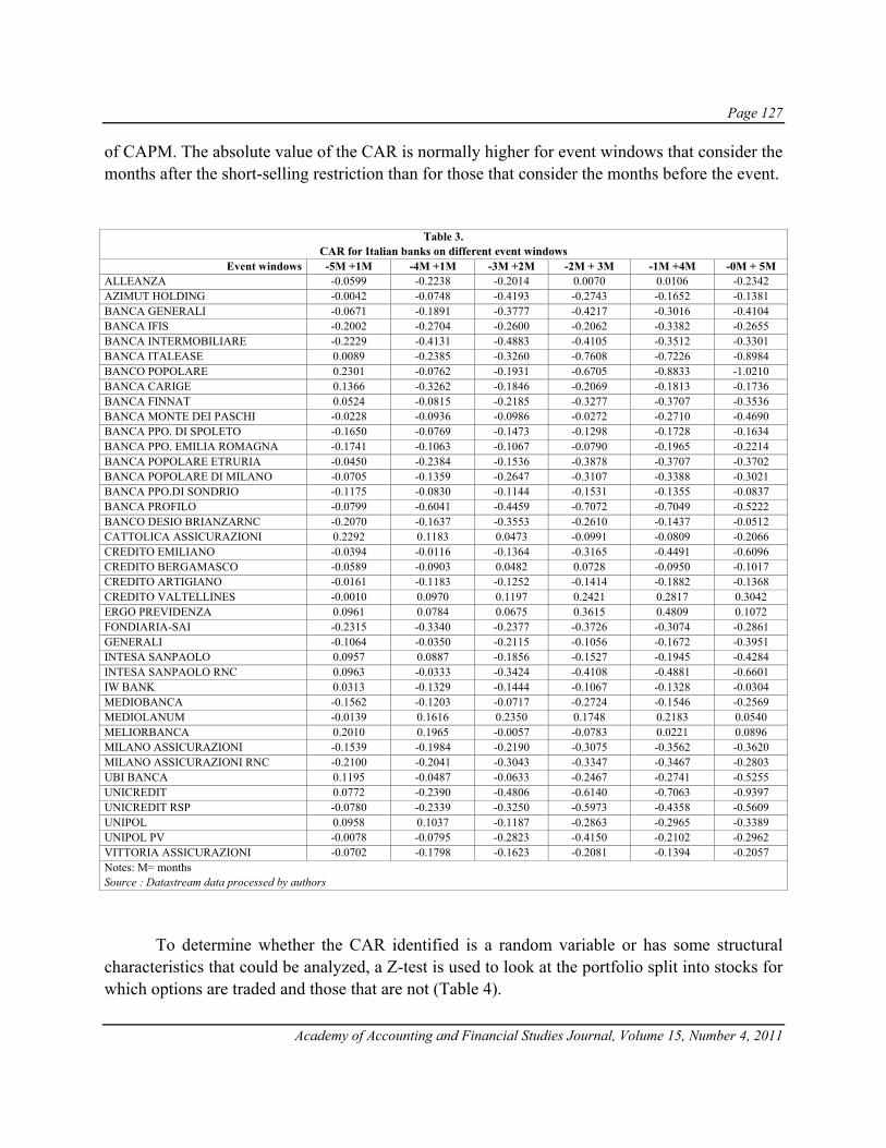
Page 127
Academy of Accounting and Financial Studies Journal, Volume 15, Number 4, 2011
of CAPM. The absolute value of the CAR is normally higher for event windows that consider the months after the short-selling restriction than for those that consider the months before the event.
Table 3. CAR for Italian banks on different event windows
Event windows -5M +1M -4M +1M -3M +2M -2M + 3M -1M +4M -0M + 5M ALLEANZA -0.0599 -0.2238 -0.2014 0.0070 0.0106 -0.2342 AZIMUT HOLDING -0.0042 -0.0748 -0.4193 -0.2743 -0.1652 -0.1381 BANCA GENERALI -0.0671 -0.1891 -0.3777 -0.4217 -0.3016 -0.4104 BANCA IFIS -0.2002 -0.2704 -0.2600 -0.2062 -0.3382 -0.2655 BANCA INTERMOBILIARE -0.2229 -0.4131 -0.4883 -0.4105 -0.3512 -0.3301 BANCA ITALEASE 0.0089 -0.2385 -0.3260 -0.7608 -0.7226 -0.8984 BANCO POPOLARE 0.2301 -0.0762 -0.1931 -0.6705 -0.8833 -1.0210 BANCA CARIGE 0.1366 -0.3262 -0.1846 -0.2069 -0.1813 -0.1736 BANCA FINNAT 0.0524 -0.0815 -0.2185 -0.3277 -0.3707 -0.3536 BANCA MONTE DEI PASCHI -0.0228 -0.0936 -0.0986 -0.0272 -0.2710 -0.4690 BANCA PPO. DI SPOLETO -0.1650 -0.0769 -0.1473 -0.1298 -0.1728 -0.1634 BANCA PPO. EMILIA ROMAGNA -0.1741 -0.1063 -0.1067 -0.0790 -0.1965 -0.2214 BANCA POPOLARE ETRURIA -0.0450 -0.2384 -0.1536 -0.3878 -0.3707 -0.3702 BANCA POPOLARE DI MILANO -0.0705 -0.1359 -0.2647 -0.3107 -0.3388 -0.3021 BANCA PPO.DI SONDRIO -0.1175 -0.0830 -0.1144 -0.1531 -0.1355 -0.0837 BANCA PROFILO -0.0799 -0.6041 -0.4459 -0.7072 -0.7049 -0.5222 BANCO DESIO BRIANZARNC -0.2070 -0.1637 -0.3553 -0.2610 -0.1437 -0.0512 CATTOLICA ASSICURAZIONI 0.2292 0.1183 0.0473 -0.0991 -0.0809 -0.2066 CREDITO EMILIANO -0.0394 -0.0116 -0.1364 -0.3165 -0.4491 -0.6096 CREDITO BERGAMASCO -0.0589 -0.0903 0.0482 0.0728 -0.0950 -0.1017 CREDITO ARTIGIANO -0.0161 -0.1183 -0.1252 -0.1414 -0.1882 -0.1368 CREDITO VALTELLINES -0.0010 0.0970 0.1197 0.2421 0.2817 0.3042 ERGO PREVIDENZA 0.0961 0.0784 0.0675 0.3615 0.4809 0.1072 FONDIARIA-SAI -0.2315 -0.3340 -0.2377 -0.3726 -0.3074 -0.2861 GENERALI -0.1064 -0.0350 -0.2115 -0.1056 -0.1672 -0.3951 INTESA SANPAOLO 0.0957 0.0887 -0.1856 -0.1527 -0.1945 -0.4284 INTESA SANPAOLO RNC 0.0963 -0.0333 -0.3424 -0.4108 -0.4881 -0.6601 IW BANK 0.0313 -0.1329 -0.1444 -0.1067 -0.1328 -0.0304 MEDIOBANCA -0.1562 -0.1203 -0.0717 -0.2724 -0.1546 -0.2569 MEDIOLANUM -0.0139 0.1616 0.2350 0.1748 0.2183 0.0540 MELIORBANCA 0.2010 0.1965 -0.0057 -0.0783 0.0221 0.0896 MILANO ASSICURAZIONI -0.1539 -0.1984 -0.2190 -0.3075 -0.3562 -0.3620 MILANO ASSICURAZIONI RNC -0.2100 -0.2041 -0.3043 -0.3347 -0.3467 -0.2803 UBI BANCA 0.1195 -0.0487 -0.0633 -0.2467 -0.2741 -0.5255 UNICREDIT 0.0772 -0.2390 -0.4806 -0.6140 -0.7063 -0.9397 UNICREDIT RSP -0.0780 -0.2339 -0.3250 -0.5973 -0.4358 -0.5609 UNIPOL 0.0958 0.1037 -0.1187 -0.2863 -0.2965 -0.3389 UNIPOL PV -0.0078 -0.0795 -0.2823 -0.4150 -0.2102 -0.2962 VITTORIA ASSICURAZIONI -0.0702 -0.1798 -0.1623 -0.2081 -0.1394 -0.2057 Notes: M= months Source : Datastream data processed by authors
To determine whether the CAR identified is a random variable or has some structural characteristics that could be analyzed, a Z-test is used to look at the portfolio split into stocks for which options are traded and those that are not (Table 4).
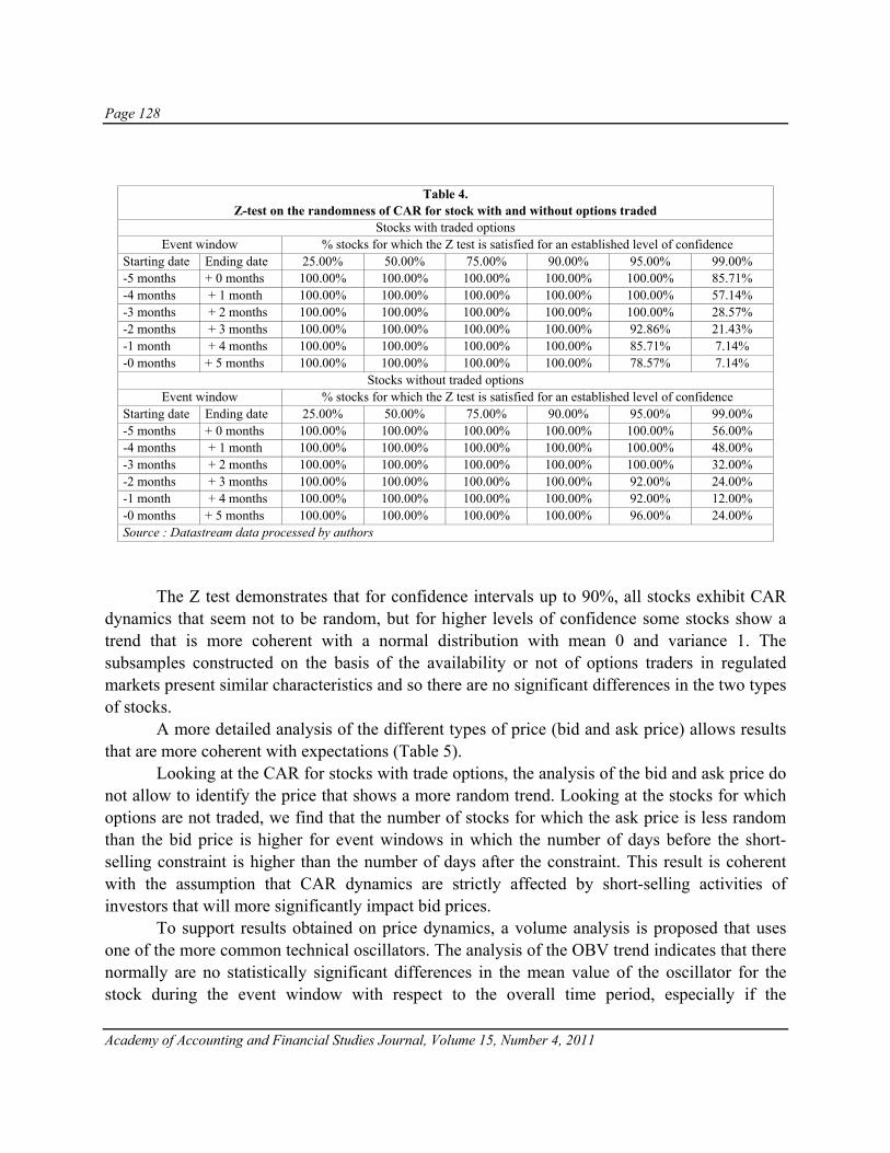
Page 128
Academy of Accounting and Financial Studies Journal, Volume 15, Number 4, 2011
Table 4. Z-test on the randomness of CAR for stock with and without options traded
Stocks with traded options Event window % stocks for which the Z test is satisfied for an established level of confidence
Starting date Ending date 25.00% 50.00% 75.00% 90.00% 95.00% 99.00% -5 months + 0 months 100.00% 100.00% 100.00% 100.00% 100.00% 85.71% -4 months + 1 month 100.00% 100.00% 100.00% 100.00% 100.00% 57.14% -3 months + 2 months 100.00% 100.00% 100.00% 100.00% 100.00% 28.57% -2 months + 3 months 100.00% 100.00% 100.00% 100.00% 92.86% 21.43% -1 month + 4 months 100.00% 100.00% 100.00% 100.00% 85.71% 7.14% -0 months + 5 months 100.00% 100.00% 100.00% 100.00% 78.57% 7.14%
Stocks without traded options Event window % stocks for which the Z test is satisfied for an established level of confidence
Starting date Ending date 25.00% 50.00% 75.00% 90.00% 95.00% 99.00% -5 months + 0 months 100.00% 100.00% 100.00% 100.00% 100.00% 56.00% -4 months + 1 month 100.00% 100.00% 100.00% 100.00% 100.00% 48.00% -3 months + 2 months 100.00% 100.00% 100.00% 100.00% 100.00% 32.00% -2 months + 3 months 100.00% 100.00% 100.00% 100.00% 92.00% 24.00% -1 month + 4 months 100.00% 100.00% 100.00% 100.00% 92.00% 12.00% -0 months + 5 months 100.00% 100.00% 100.00% 100.00% 96.00% 24.00% Source : Datastream data processed by authors
The Z test demonstrates that for confidence intervals up to 90%, all stocks exhibit CAR dynamics that seem not to be random, but for higher levels of confidence some stocks show a trend that is more coherent with a normal distribution with mean 0 and variance 1. The subsamples constructed on the basis of the availability or not of options traders in regulated markets present similar characteristics and so there are no significant differences in the two types of stocks.
A more detailed analysis of the different types of price (bid and ask price) allows results that are more coherent with expectations (Table 5).
Looking at the CAR for stocks with trade options, the analysis of the bid and ask price do not allow to identify the price that shows a more random trend. Looking at the stocks for which options are not traded, we find that the number of stocks for which the ask price is less random than the bid price is higher for event windows in which the number of days before the short-selling constraint is higher than the number of days after the constraint. This result is coherent with the assumption that CAR dynamics are strictly affected by short-selling activities of investors that will more significantly impact bid prices.
To support results obtained on price dynamics, a volume analysis is proposed that uses one of the more common technical oscillators. The analysis of the OBV trend indicates that there normally are no statistically significant differences in the mean value of the oscillator for the stock during the event window with respect to the overall time period, especially if the

Page 129
Academy of Accounting and Financial Studies Journal, Volume 15, Number 4, 2011
confidence level is higher than 25%. All other results obtained on OBV are not clearly explainable on the basis of short-selling strategies, even if the sample is split into stocks with or without options traded (Table 6).
Table 5 Z-test comparison between stock dynamics before and after the definition of the short sale constraints looking at
bid and ask prices Stocks with traded options – Bid price
Event window % stocks for which the Z test is satisfied for an established level of confidence Starting date Ending date 25.00% 50.00% 75.00% 90.00% 95.00% 99.00%
-5 months + 0 months 100.00% 100.00% 100.00% 100.00% 100.00% 85.71% -4 months + 1 month 100.00% 100.00% 100.00% 100.00% 100.00% 57.14% -3 months + 2 months 100.00% 100.00% 100.00% 100.00% 100.00% 28.57% -2 months + 3 months 100.00% 100.00% 100.00% 100.00% 100.00% 35.71% -1 month + 4 months 100.00% 100.00% 100.00% 100.00% 92.86% 21.43% -0 months + 5 months 100.00% 100.00% 100.00% 100.00% 85.71% 14.29%
Stocks with traded options – Ask price Event window % stocks for which the Z test is satisfied for an established level of confidence
Starting date ending date 25.00% 50.00% 75.00% 90.00% 95.00% 99.00% -5 months + 0 months 100.00% 100.00% 100.00% 100.00% 100.00% 78.57% -4 months + 1 month 100.00% 100.00% 100.00% 100.00% 100.00% 57.14% -3 months + 2 months 100.00% 100.00% 100.00% 100.00% 100.00% 28.57% -2 months + 3 months 100.00% 100.00% 100.00% 100.00% 100.00% 35.71% -1 month + 4 months 100.00% 100.00% 100.00% 100.00% 92.86% 42.86% -0 months + 5 months 100.00% 100.00% 100.00% 100.00% 85.71% 21.43%
Stocks without option traded - Bid price Event window % stocks for which the Z test is satisfied for an established level of confidence
Starting date Ending date 25.00% 50.00% 75.00% 90.00% 95.00% 99.00% -5 months + 0 months 96.00% 96.00% 96.00% 96.00% 96.00% 56.00% -4 months + 1 month 96.00% 96.00% 96.00% 96.00% 96.00% 48.00% -3 months + 2 months 96.00% 96.00% 96.00% 96.00% 96.00% 28.00% -2 months + 3 months 96.00% 96.00% 96.00% 96.00% 92.00% 20.00% -1 month + 4 months 96.00% 96.00% 96.00% 96.00% 88.00% 8.00% -0 months + 5 months 96.00% 96.00% 96.00% 96.00% 84.00% 20.00%
Stocks without traded options - Ask price Event window % stocks for which the Z test is satisfied for an established level of confidence
Starting date Ending date 25.00% 50.00% 75.00% 90.00% 95.00% 99.00% -5 months + 0 months 96.00% 96.00% 96.00% 96.00% 96.00% 48.00% -4 months + 1 month 96.00% 96.00% 96.00% 96.00% 96.00% 36.00% -3 months + 2 months 96.00% 96.00% 96.00% 96.00% 96.00% 16.00% -2 months + 3 months 96.00% 96.00% 96.00% 96.00% 92.00% 12.00% -1 month + 4 months 96.00% 96.00% 96.00% 96.00% 88.00% 8.00% -0 months + 5 months 96.00% 96.00% 96.00% 96.00% 88.00% 12.00%
SOURCE: DATASTREAM DATA PROCESSED BY AUTHORS
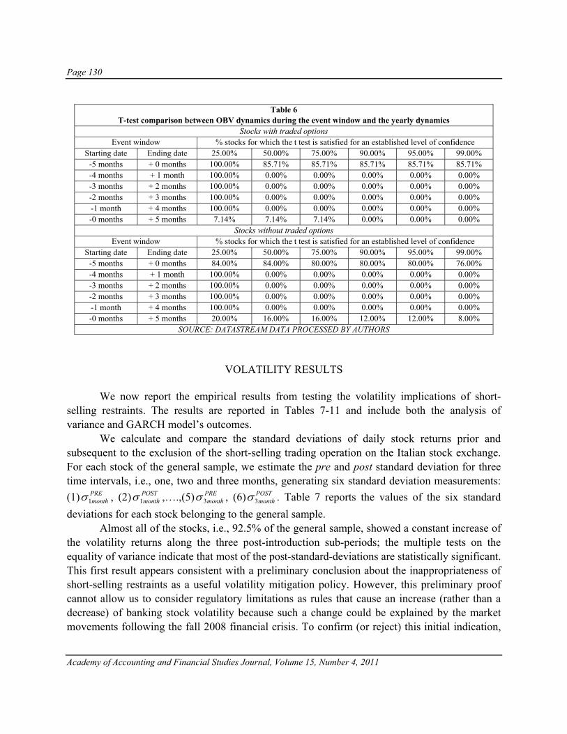
Page 130
Academy of Accounting and Financial Studies Journal, Volume 15, Number 4, 2011
Table 6
T-test comparison between OBV dynamics during the event window and the yearly dynamics Stocks with traded options
Event window % stocks for which the t test is satisfied for an established level of confidence Starting date Ending date 25.00% 50.00% 75.00% 90.00% 95.00% 99.00%
-5 months + 0 months 100.00% 85.71% 85.71% 85.71% 85.71% 85.71% -4 months + 1 month 100.00% 0.00% 0.00% 0.00% 0.00% 0.00% -3 months + 2 months 100.00% 0.00% 0.00% 0.00% 0.00% 0.00% -2 months + 3 months 100.00% 0.00% 0.00% 0.00% 0.00% 0.00% -1 month + 4 months 100.00% 0.00% 0.00% 0.00% 0.00% 0.00% -0 months + 5 months 7.14% 7.14% 7.14% 0.00% 0.00% 0.00%
Stocks without traded options Event window % stocks for which the t test is satisfied for an established level of confidence
Starting date Ending date 25.00% 50.00% 75.00% 90.00% 95.00% 99.00% -5 months + 0 months 84.00% 84.00% 80.00% 80.00% 80.00% 76.00% -4 months + 1 month 100.00% 0.00% 0.00% 0.00% 0.00% 0.00% -3 months + 2 months 100.00% 0.00% 0.00% 0.00% 0.00% 0.00% -2 months + 3 months 100.00% 0.00% 0.00% 0.00% 0.00% 0.00% -1 month + 4 months 100.00% 0.00% 0.00% 0.00% 0.00% 0.00% -0 months + 5 months 20.00% 16.00% 16.00% 12.00% 12.00% 8.00%
SOURCE: DATASTREAM DATA PROCESSED BY AUTHORS
VOLATILITY RESULTS
We now report the empirical results from testing the volatility implications of short-selling restraints. The results are reported in Tables 7-11 and include both the analysis of variance and GARCH model’s outcomes.
We calculate and compare the standard deviations of daily stock returns prior and subsequent to the exclusion of the short-selling trading operation on the Italian stock exchange. For each stock of the general sample, we estimate the pre and post standard deviation for three time intervals, i.e., one, two and three months, generating six standard deviation measurements: (1) PRE
month1σ , (2) POSTmonth1σ ,….,(5) PRE
month3σ , (6) POSTmonth3σ . Table 7 reports the values of the six standard
deviations for each stock belonging to the general sample. Almost all of the stocks, i.e., 92.5% of the general sample, showed a constant increase of
the volatility returns along the three post-introduction sub-periods; the multiple tests on the equality of variance indicate that most of the post-standard-deviations are statistically significant. This first result appears consistent with a preliminary conclusion about the inappropriateness of short-selling restraints as a useful volatility mitigation policy. However, this preliminary proof cannot allow us to consider regulatory limitations as rules that cause an increase (rather than a decrease) of banking stock volatility because such a change could be explained by the market movements following the fall 2008 financial crisis. To confirm (or reject) this initial indication,

Page 131
Academy of Accounting and Financial Studies Journal, Volume 15, Number 4, 2011
an inspection of the first and second control procedures’ results seems to be indispensable (see section 3.2.2.1).
Table 7 Volatility Analysis: the comparison between pre and post standard deviation
PRE-restriction perioda POST-restriction perioda Volatility change b Stockc PRE
month3σ PREmonth2σ PRE
month1σ POSTmonth3σ POST
month2σ POSTmonth1σ +3Md +2Md 1Md
ALLEANZA A.c 2.016**e 2.1394** 2.3552** 4.077** 4.1424** 4.4008** AZIMUT H. 3.4105** 3.4528* 4.0808 4.7274** 4.9472* 5.0781 B.CA GENERALI 2.2544* 2.3589* 2.4544* 3.0103* 3.2908* 3.8777* BANCA IFIS 1.8139** 1.7386** 1.8134* 2.5097** 2.7422** 3.0029* B.CA INTERM. 1.2452** 1.0685** 1.3964 2.1232** 2.2858** 1.9205 BANCA ITAL. 4.1478** 3.0490** 3.3878** 6.1042** 6.4726** 8.4056** B.CO POPOL. 2.6719** 2.7671** 3.0564** 5.4872** 5.4891** 6.5398** B.CA CARIGE 3.2136** 3.5568* 4.3546 4.6928** 4.8237* 4.7581 B.CA CARIGE R. 2.5197** 2.7430** 2.9752 3.8040** 4.3305** 3.9117 B.CA FINNAT 1.7056** 1.4986** 1.8448** 3.5053** 3.998** 4.0574** B.CA MPS 2.8131 2.7454 3.4730 3.2011 3.395 3.2542 POP. DI SP.TO 1.8578** 1.5597** 1.2286** 3.3053** 3.7001** 4.2051** POP. EMIL ROM. 2.2248 2.1274* 2.3402* 2.6863 3.1041* 3.8687* POP. ETRUR. L. 1.9036** 1.9064** 2.0738** 2.9352** 3.3603** 3.7386** POP. MILANO 2.8358** 3.0345** 3.7596* 4.9261** 5.8472** 7.2592* POP. SONDRIO 1.1002** 1.0738** 1.4478** 3.0991** 3.6654** 4.8162** B.CA PROFILO 2.6539** 2.1801** 2.2674** 4.5981** 5.3108** 6.1867** B.CO DESIOB. R. 2.8618 2.5326 2.2717 3.0833 2.8214 3.0495 CATTOLICA ASS 2.5110* 2.7927 3.0168 3.3327* 3.7566 4.3561 CR BERGAM.CO 2.5937 2.5499* 2.1312** 3.0785 3.5460* 4.1385** CREDEM 2.4580** 2.6754* 3.0702 3.3985** 3.9561* 4.6591 CR. ARTIGIANO 2.0996 2.2892 2.2023* 2.4467 2.7254 3.4711* CR. VALTELL.SE 1.8163** 1.8858** 2.3034** 3.4903** 3.2469** 4.1124** ERGO PREV.ZA 3.1073** 2.5805** 2.9924** 0.8814** 0.2485** 0.2486** FOND. SAI 2.4872** 2.5622** 2.9522** 4.7023** 5.4393** 6.6547** GENERALI ASS 1.7481** 1.9976* 2.5154 2.6040** 2.7447* 2.5399 INTESA SANP. 2.6967** 3.0392** 3.5346** 6.3150** 7.0645** 6.2833** INT-SANP. R. 2.4447** 2.6506** 2.8131** 6.5139** 7.5489** 8.6173** IW BANK 1.3439** 1.0988** 1.0999** 2.1237** 2.3765** 2.4972** MEDIOBANCA 2.0671 2.2493 2.3737 2.1087 1.9904 1.9982 MEDIOLANUM 3.2311 3.2804 3.5816 3.3889 3.9660 4.7172 MELIORBANCA 0.9545** 0.8617** 1.1194** 2.1115** 2.5482** 3.4332** MILANO ASS 2.1638** 2.1129** 2.1882** 3.9573** 4.6037** 5.1207** MILANO ASS R. 2.0289**- 1.9554** 2.3537** 3.3997** 3.8871** 4.4365** UBI BANCA 2.0564** 2.1392** 2.4641** 3.9136** 4.2687** 4.5720** UNICREDIT 2.9387** 3.0810 3.8379** 7.1332** 7.9742 8.2601** UNICREDIT RISP 2.2449** 2.4151** 2.8250 4.0628** 4.5527** 5.2425 UNIPOL 2.1354** 2.0437** 2.4575** 3.8016** 4.1307** 5.2123** UNIPOL PRIV 2.4228** 2.0531** 2.9796** 5.0451** 5.6795** 6.7990** VITTORIA ASS 2.0526** 2.1751* 2.6724* 3.0655** 3.1798* 3.6705
Numbers of stock with volatility up ( ) 39 38 37 Numbers of stock with volatility down ( ) 1 2 3
Standard deviation average change for stock with derivatives 73.30% 86.70% 79.90% Standard deviation average change for stock without derivatives 50.60% 96.90% 110.7%
Notes: aDate of restriction on short selling trading : September, 23rd 2008 bBold arrows indicates time-constant volatility change cBold/italic name indicates stock underlying of derivative contracts.
d n° months after the introduction of restrictions e Value multiplied by 102 for readability * significant at the 5% ** significant at 1% Source : Datastream data processed by authors

Page 132
Academy of Accounting and Financial Studies Journal, Volume 15, Number 4, 2011
With regard to the first control procedure, which provides a volatility comparison
between stock with and without derivatives listed contracts, the interpretation of a short-sales ban as a volatility trigger would be confirmed if most of the underlying stock of derivatives trading (reported in Table 2) would exhibit a different sign of the change in volatility with respect to stocks not subject to derivatives contracts. Because derivatives trading provides alternative trading strategies to assume a short position on stocks for which short-selling is impracticable, if
Table 8 Equality of Variance Test for 3months before and after short selling restriction on daily returns (closing price)a
F-test Bartelett Levene Brown-Forsytheb F-test Bartelett Levene Brown-
Forsytheb
ALLEANZA ASS 0.2445 (0.0000)c
0.4151 (0.519)
0.0157 (0.900)
0.01372 (0.906) CREDEM 0.5231
(0.0097) 4.2939 (0.038)
2.545 (0.113)
2.790 (0.097)
AZIMUT H. 0.5205 (0.0092)
0.7583 (0.384)
0.4551 (0.501)
0.4574 (0.499) CR. ARTIGIANO 0.7364
(0.2193) 13.4051 (0.000)
7.7651 (0.006)
7.3859 (0.007)
B.CA GENERALI 0.5608 (0.0208)
7.2431 (0.007)
3.9513 (0.048)
3.886 (0.049) CR. VALTELL.SE 0.2708
(0.0000) 0.1406 (0.708)
0.5889 (0.444)
0.6438 (0.424)
BANCA IFIS 0.9952 ( 0.0096)
0.7304 (0.393)
0.0234 (0.878)
0.0299 (0.862) ERGO PREV.ZA 12.4286
(0.0000) 5.9900 (0.014)
2.6951 0.103
1.227 (0.270)
B.CA INTERM. 0.3440 (0.0000)
0.6027 (0.438)
0.0177 (0.894)
0.0286 (0.866) FONDIARIA-SAI 0.2798
(0.0000 ) 6.8542 (0.009)
0.5487 (0.460)
0.5389 (0.464)
BANCA ITALEASE 0.4617 (0.0021)
6.2593 (0.012)
1.7217 (0.191)
1.7208 (0.191) GENERALI ASS 0.4507
( 0.0015) 0.4977 (0.481)
1.2430 (0.266)
1.1675 (0.282)
B.CO POPOLARE 0.2371 (0.0000)
0.1981 (0.656)
0.0470 (0.828)
0.0028 (0.957) INTESA SANP. 0.1824
(0.0000) 1.2548 (0.263)
0.4269 (0.515)
0.4884 (0.486)
B.CA CARIGE 0.4690 (0.0026)
1.3426 (0.247)
0.6842 (0.409)
0.5818 (0.446)
INTESA SANP. R.
0.1409 (0.0000)
5.1504 (0.023)
0.4096 (0.523)
0.4108 (0.522)
B.CA CARIGE R. 0.4388 (0.0011)
3.5303 (0.060)
1.6610 (0.199)
1.8318 (0.178) IW BANK 0.4005
( 0.0003) 1.4384 (0.230)
0.0652 (0.799)
0.0765 (0.782)
B.CA FINNAT 0.2368 ( 0.0000 )
0.0322 (0.858)
0.0682 (0.794)
0.0529 (0.818) MEDIOBANCA 0.9610
(0.8720) 0.8202 (0.365)
0.1846 (0.668)
0.2763 (0.599)
B.CA MPS 0.7723 (0.2993)
2.6023 (0.107)
0.6617 (0.417)
0.6145 (0.434) MEDIOLANUM 0.9091
(0.7009) 24.4637 (0.000)
20.108 (0.000)
20.0966 (0.000)
POP. DI SP.TO 0.3159 (0.0000)
2.7751 (0.096)
1.5161 (0.220)
1.8455 (0.176) MELIORBANCA 0.2043
(0.000) 55.6500 (0.000)
9.8286 (0.002)
9.4641 (0.002)
POP. EMIL ROM. 0.6859 (0.1306)
7.7324 (0.005)
(3.6194) (0.059)
3.7556 (0.0547) MILANO ASS 0.2990
(0.0000) 8.6809 (0.003)
4.1812 (0.043)
4.1583 (0.043)
POP. ETRUR. L. 0.4206 (0.0006)
6.9157 (0.009)
4.7764 (0.030)
4.6001 (0.033) MILANO ASS R. 0.3561
(0.0000) 2.9894 (0.084)
0.3426 (0.559)
0.2904 (0.591)
POP. MILANO 0.3314 (0.0000)
34.057 (0.000)
11.9055 (0.000)
11.9134 (0.000) UBI BANCA 0.2761
(0.0000) 3.8598 (0.049)
1.3611 (0.245)
1.3571 (0.246)
POP. SONDRIO 0.1260 (0.000)
24.511 (0.000)
1.3679 (0.244)
1.1685 (0.282) UNICREDIT 0.1697
(0.0000) 1.0081 (0.315)
0.3630 (0.548)
0.3627 (0.548)
B.CA PROFILO 0.3331 (0.0000)
9.7909 ( 0.002)
4.1932 (0.042)
4.1903 (0.043) UNICREDIT RISP 0.3053
(0.0000) 0.2978 (0.585)
0.0157 (0.900)
0.0056 (0.940)
B.CO DESIO B. R. 0.8615 (0.5485)
3.6557 (0.056)
0.2307 (0.632)
0.2400 (0.625) UNIPOL 0.3155
(0.0000) 4.5754 (0.032)
1.0278 (0.312)
1.0407 (0.309)
CATTOLICA ASS 0.5677 (0.0236)
4.5057 (0.034)
0.8541 (0.357)
0.8529 (0.357) VITTORIA ASS 0.4483
(0.0014 ) 1.5895 (0.207)
0.3772 (0.540)
0.335 (0.563)
CR BERGAM.CO 0.7099 (0.1691)
26.3458 (0.000)
14.1855 (0.000)
14.256 (0.000)
Notes: athe tables of 1-month and 2-month subperiod are omitted for brevity bBrown and Forsy statistic replace the mean with the median in Levene's formula. cNumbers in parentheses represent p-value Source : Datastream data processed by authors
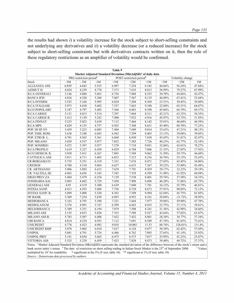
Page 133
Academy of Accounting and Financial Studies Journal, Volume 15, Number 4, 2011
the results had shown i) a volatility increase for the stock subject to short-selling constraints and not underlying any derivatives and ii) a volatility decrease (or a reduced increase) for the stock subject to short-selling constraints but with derivatives contracts written on it, then the role of these regulatory restrictions as an amplifier of volatility would be confirmed.
Table 9 Market Adjusted Standard Deviation (MktAdjSD)a of daily data
PRE-restriction periodb POST-restriction periodb Volatility change Stock -3M - 2M -1M +3M +2M +1M +3M +2M 1M ALLEANZA ASS 4.830c 4.643 5.535 6.987 7.254 8.183 44.66% 56.24% 47.84% AZIMUT H. 4.824 4.259 4.770 7.573 7.635 8.013 56.99% 79.27% 67.99% B.CA GENERALI 5.146 4.886 5.863 6.726 7.068 8.353 30.70% 44.66% 42.47% BANCA IFIS 4.836 4.520 5.288 7.007 7.567 8.135 44.89% 67.41% 53.84% B.CA INTERM. 5.525 5.166 5.995 6.824 7.204 8.369 23.51% 39.45% 39.60% B.CA ITALEASE 5.973 4.630 5.602 7.337 7.663 9.348 22.84% 65.51% 66.87% B.CO POPOLARE 5.187 4.797 5.485 7.566 8.001 9.290 45.86% 66.79% 69.37% B.CA CARIGE 5.131 4.815 5.514 7.297 7.864 8.511 42.21% 63.32% 54.35% B.CA CARIGE R. 5.412 5.159 5.242 7.900 7.932 6.916 45.97% 53.75% 31.93% B.CA FINNAT 5.233 5.023 5.639 7.112 7.464 8.142 35.91% 48.60% 44.39% B.CA MPS 4.829 4.155 4.757 6.925 7.508 8.431 43.40% 80.70% 77.23% POP. DI SP.TO 5.459 5.223 6.085 7.404 7.689 9.014 35.63% 47.21% 48.13% POP. EMIL ROM. 5.638 5.248 6.043 6.942 7.299 8.403 23.13% 39.08% 39.05% POP. ETRUR. L. 4.781 4.565 5.361 6.868 6.930 7.638 43.65% 51.81% 42.47% POP. MILANO 5.029 4.537 5.077 7.052 7.385 7.726 40.23% 62.77% 52.18% POP. SONDRIO 5.472 5.397 5.077 7.270 7.718 9.051 32.86% 43.01% 78.27% B.CA PROFILO 5.619 5.327 6.450 6.829 6.768 7.606 21.53% 27.05% 17.92% B.CO DESIO B. R. 5.930 5.431 6.267 7.803 7.589 9.062 31.59% 39.73% 44.60% CATTOLICA ASS 5.011 4.711 5.403 6.853 7.215 8.236 36.76% 53.15% 52.43% CR BERGAM.CO 5.735 5.351 6.319 7.331 7.676 8.471 27.83% 43.45% 34.06% CREDEM 4.760 4.310 5.064 6.627 6.633 7.367 39.22% 53.90% 45.48% CR. ARTIGIANO 5.906 5.892 6.415 7.629 7.791 8.929 29.17% 32.23% 39.19% CR. VALTELL.SE 4.963 4.656 5.343 7.543 7.539 8.599 51.98% 61.92% 60.94% ERGO PREV.ZA 5.494 5.479 6.254 7.129 7.538 8.401 29.76% 37.58% 34.33% FONDIARIA-SAI 5.093 4.602 5.729 7.450 7.909 9.496 46.28% 71.86% 65.75% GENERALI ASS 4.95 4.519 5.300 6.639 7.040 7.781 34.12% 55.79% 46.81% INTESA SANP. 4.913 4.593 5.009 7.758 8.729 8.672 57.91% 90.05% 73.13% INTESA SANP. R. 5.099 5.008 5.520 8.303 7.299 9.994 62.84% 45.75% 81.05% IW BANK 5.309 7.254 5.830 6.893 4.953 8.101 29.84% -31.72% 38.95% MEDIOBANCA 5.163 4.793 5.398 7.221 7.664 7.977 39.86% 59.90% 47.78% MEDIOLANUM 5.376 4.991 5.747 6.599 6.843 8.035 22.75% 37.11% 39.81% MELIORBANCA 5.389 5.251 6.194 7.079 7.508 8.341 31.36% 42.98% 34.66% MILANO ASS 5.155 4.833 5.828 7.353 7.589 9.527 42.64% 57.02% 63.47% MILANO ASS R. 5.783 5.507 6.408 7.422 7.422 8.801 28.34% 34.77% 37.34% UBI BANCA 4.814 4.234 4.953 7.112 7.691 8.589 47.74% 81.65% 73.41% UNICREDIT 4.778 4.423 4.982 9.018 10.085 11.53 88.74% 128.01% 131.4% UNICREDIT RISP 5.078 5.002 6.010 7.637 8.124 9.477 50.39% 62.42% 57.69% UNIPOL 5.081 4.791 5.724 6.486 6.762 7.093 27.65% 41.14% 23.92% UNIPOL PRIV 5.141 4.654 5.665 6.475 6.573 7.017 25.95% 41.23% 23.87% VITTORIA ASS 5.325 5.229 6.459 7.423 7.829 8.873 39.40% 49.72% 37.37% Notes: a Market Adjusted Standard Deviation (MktAdjSD) represents the standard deviation of the difference between of the stock’s return and a bank sector index’s return. b The date of restriction on short selling trading in Italian Stock Market is the 23th of September 2008. c Values multiplied by 102 for readability * significant at the 5% (F-test, table 10) ** significant at 1% (F-test, table 10) Source : Datastream data processed by authors

Page 134
Academy of Accounting and Financial Studies Journal, Volume 15, Number 4, 2011
The evidence from the first control procedure reported in Table 7 shows that in 13 of 15 cases, the underlying stock of listed derivatives contracts shows a statistically significant increase in volatility along each of the three post-restriction sub-periods. These results seem to counter our preliminary idea that short sales bans can increase the market volatility of affected stocks.
Table 10 Test of Equality of Variance for Market Adjusted Standard Deviation (MktAdjSD)
-3M +3M -2M +2M -1M +1M Stock F-test p-value F-test p-value F-test p-value ALLEANZA ASS 0.4780 0.0033 0.4097 0.0039 0.4574 0.0753 AZIMUT HOLDING 0.4057 0.0004 0.3113 0.0002 0.3544 0.0193 BANCA GENERALI 0.5854 0.0322 0.4779 0.0165 0.4928 0.1068 BANCA IFIS 0.4764 0.0032 0.3569 0.0009 0.4226 0.0507 BANCA INTERMOBILIARE 0.6555 0.0905 0.5142 0.0304 0.5131 0.1279 BANCA ITALEASE 0.6626 0.0990 0.3651 0.0012 0.3591 0.0209 BANCO POPOLARE 0.4700 0.0027 0.3595 0.0010 0.3486 0.0176 BCA CARIGE 0.4945 0.0050 0.3749 0.0016 0.4198 0.0490 BCA CARIGE RISP 0.4693 0.0026 0.4231 0.0054 0.5744 0.2047 BCA FINNAT 0.5414 0.0143 0.4529 0.0102 0.4797 0.0944 BCA MPS 0.4864 0.0041 0.3064 0.0002 0.3184 0.0102 BCA POP DI SPOLETO 0.5437 0.0150 0.4615 0.0121 0.4557 0.0740 BCA POP EMIL ROMAGNA 0.6596 0.0954 0.5170 0.0317 0.5172 0.1324 BCA POP ETRUR-LAZIO 0.4846 0.0039 0.4339 0.0068 0.4927 0.1067 BCA POP MILANO 0.5086 0.0070 0.3774 0.0017 0.4320 0.0567 BCA POP SONDRIO 0.5666 0.0232 0.4890 0.0200 0.3147 0.0095 BCA PROFILO 0.6770 0.1178 0.6194 0.1175 0.7191 0.4484 BCO DESIO BRIA RISP 0.5776 0.0282 0.5122 0.0295 0.4783 0.0931 CATTOLICA ASS 0.5348 0.0125 0.4264 0.0058 0.4305 0.0557 CR BERGAMASCO 0.6119 0.0493 0.4860 0.0190 0.5565 0.1804 CREDEM 0.5161 0.0083 0.4223 0.0053 0.4725 0.0879 CREDITO ARTIGIANO 0.5992 0.0404 0.5719 0.0682 0.5162 0.1314 CREDITO VALTELLINESE 0.4329 0.0009 0.3814 0.0019 0.3861 0.0314 ERGO PREVIDENZA 0.5939 0.0371 0.5284 0.0377 0.5542 0.1773 FONDIARIA-SAI 0.4673 0.0025 0.3386 0.0005 0.3641 0.0226 GENERALI ASS 0.5558 0.0190 0.4120 0.0041 0.4640 0.0807 INTESA SANPAOLO 0.4010 0.0003 0.2769 0.0000 0.3336 0.0135 INTESA SANPAOLO RISP 0.3771 0.0001 0.4707 0.0144 0.3050 0.0078 IW BANK 0.5933 0.0367 2.1447 0.0132 0.4579 0.0757 MEDIOBANCA 0.5112 0.0075 0.3912 0.0024 0.5115 0.1262 MEDIOLANUM 0.6637 0.1003 0.5321 0.0398 0.5514 0.1737 MELIORBANCA 0.5795 0.0291 0.4890 0.0201 0.3743 0.0264 MILANO ASS 0.4916 0.0047 0.4055 0.0035 0.3743 0.0264 MILANO ASS RISP 0.6072 0.0667 0.5505 0.0516 0.5302 0.1474 UBI BANCA 0.4583 0.0019 0.3031 0.0001 0.3326 0.0133 UNICREDIT 0.2808 0.0000 0.1924 0.0000 0.1865 0.0002 UNICREDIT RISP 0.4421 0.0012 0.3792 0.0018 0.4022 0.0391 UNIPOL 0.6137 0.0506 0.5020 0.0250 0.6513 0.3253 UNIPOL PRIV 0.6303 0.0645 0.5013 0.0247 0.6519 0.3264 VITTORIA ASS 0.5147 0.0081 0.4460 0.0089 0.5298 0.1470 Source : Datastream data processed by authors

Page 135
Academy of Accounting and Financial Studies Journal, Volume 15, Number 4, 2011
However, average changes in the standard deviation suggest the importance of a deeper investigation about the role of short sales because, with the exception of the three-month case, the values reported at the bottom of Table 7 exhibit a greater variation of post-ban standard deviations for stocks without a derivatives contract than those with one. This evidence encourages us to perform a closer examination through the implementation of a second control procedure.
The second control procedure consists of an estimation of pre and post MktAdjSD values for each of the ith stock of the general sample along the usual three sub-periods.
The results are reported in Table 9: In 39 out of 40 cases (97.5%), the MktAdjSD variable shows a constant increase over 1, 2 and 3 months after the introduction of bans on short-selling practices.
This evidence, which is corroborated by overall statistical significance (see Table 10), seems to confirm the previous conclusion regarding the presence of a volatility effect exclusively related to the abolition of short-selling practice because there is a lack of relationship between the volatility returns of the general sample and the volatility returns of the overall banking sector. As described in section [3.2.2.1], the MktAdjSDi measure represents the standard deviation of the excess return between the ith stock’s returns and the bank index’s return. Therefore, an increase in MktAdjSDi can be explained by a decrease in the correlation coefficients between the returns of ith stock and the bank sector index. In this case, the overall increase in volatility occurring after the introduction of constraints on short-selling operations could be judged as an effect caused by the policy decision to put a ban on naked short sales rather than a likely reaction to a global movement of bank shares around the markets.
The results shown in Table 11 refer to estimates of the coefficients in equation (6) for a period ranging from January 2nd, 2008 to March 3rd, 2009. At first glance, the results seem to confirm what is reported by ANOVA approach. However, it is evident from the table that almost all of the data are not statistically significant, so these points of view can always be discarded. The loss of significance is probably related to the low number/frequency of data even though a longer time period was considered. Regardless of statistical significance, from the data contained in Table 11, we recognize that in 33 out of 40 cases, the sign of the γ1 variable is positive and preliminarily consistent with the idea of connecting the volatility growth to the short-selling bans.
To assess whether the relationship between the volatility increase and the regulator’s intervention in short-selling practices is appropriate, we submitted the GARCH analysis to the two control procedures provided in the previous section10. The first procedure is designed to compare the sign of the dummy coefficients between stocks that are underlying the derivatives and the other. In fact, in the presence of an impact on the volatility due exclusively to the regulator’s intervention, we expected a sign difference in the variable γ1 between stocks with and without derivatives contracts (option contracts, for example), as speculative positions could have been achieved on the derivatives markets.
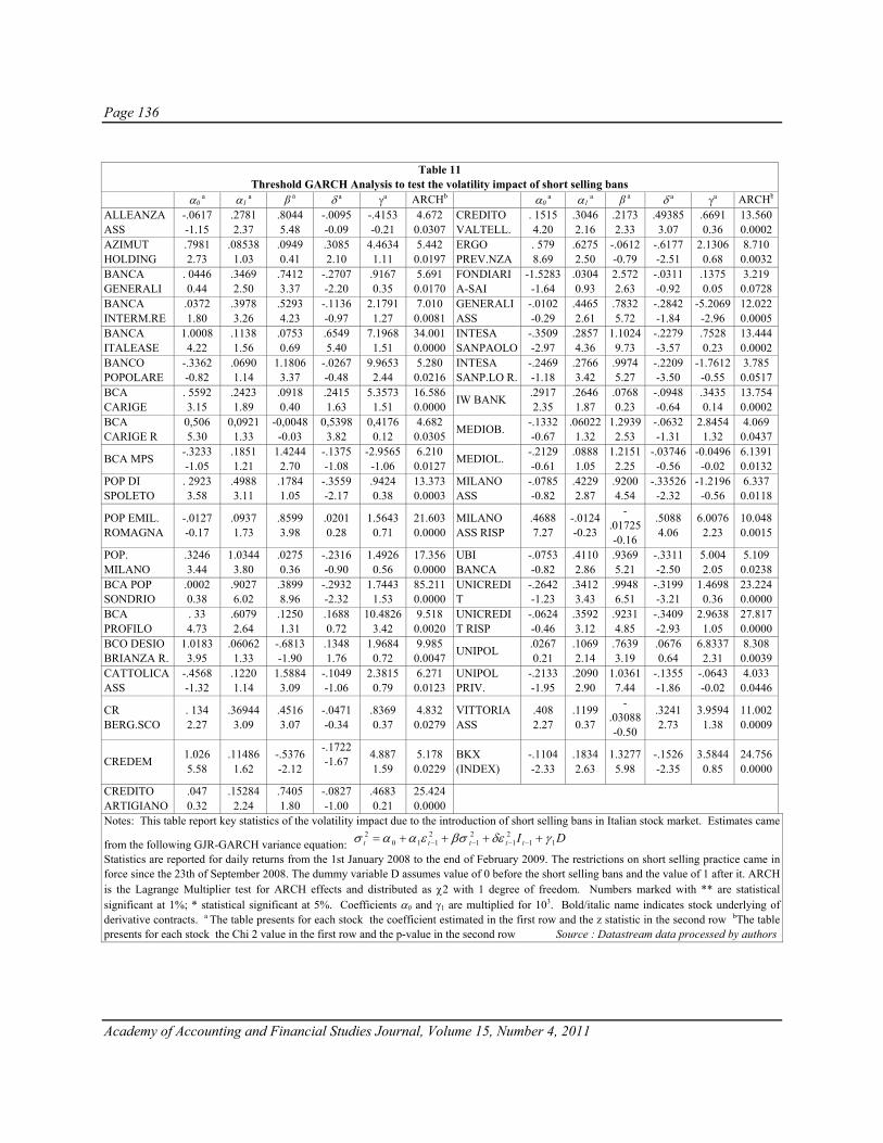
Page 136
Academy of Accounting and Financial Studies Journal, Volume 15, Number 4, 2011
Table 11
Threshold GARCH Analysis to test the volatility impact of short selling bans α0
a α1 a β a δ a γa ARCHb α0
a α1a β a δ a γa ARCHb
ALLEANZA ASS
-.0617 -1.15
.2781 2.37
.8044 5.48
-.0095 -0.09
-.4153 -0.21
4.672 0.0307
CREDITO VALTELL.
. 1515 4.20
.3046 2.16
.2173 2.33
.49385 3.07
.6691 0.36
13.560 0.0002
AZIMUT HOLDING
.7981 2.73
.08538 1.03
.0949 0.41
.3085 2.10
4.4634 1.11
5.442 0.0197
ERGO PREV.NZA
. 579 8.69
.6275 2.50
-.0612 -0.79
-.6177 -2.51
2.1306 0.68
8.710 0.0032
BANCA GENERALI
. 0446 0.44
.3469 2.50
.7412 3.37
-.2707 -2.20
.9167 0.35
5.691 0.0170
FONDIARIA-SAI
-1.5283-1.64
.0304 0.93
2.572 2.63
-.0311 -0.92
.1375 0.05
3.219 0.0728
BANCA INTERM.RE
.0372 1.80
.3978 3.26
.5293 4.23
-.1136 -0.97
2.1791 1.27
7.010 0.0081
GENERALI ASS
-.0102 -0.29
.4465 2.61
.7832 5.72
-.2842 -1.84
-5.2069-2.96
12.022 0.0005
BANCA ITALEASE
1.0008 4.22
.1138 1.56
.0753 0.69
.6549 5.40
7.1968 1.51
34.001 0.0000
INTESA SANPAOLO
-.3509 -2.97
.2857 4.36
1.1024 9.73
-.2279 -3.57
.7528 0.23
13.444 0.0002
BANCO POPOLARE
-.3362 -0.82
.0690 1.14
1.1806 3.37
-.0267 -0.48
9.9653 2.44
5.280 0.0216
INTESA SANP.LO R.
-.2469 -1.18
.2766 3.42
.9974 5.27
-.2209 -3.50
-1.7612-0.55
3.785 0.0517
BCA CARIGE
. 5592 3.15
.2423 1.89
.0918 0.40
.2415 1.63
5.3573 1.51
16.586 0.0000 IW BANK .2917
2.35 .2646 1.87
.0768 0.23
-.0948 -0.64
.3435 0.14
13.754 0.0002
BCA CARIGE R
0,506 5.30
0,0921 1.33
-0,0048 -0.03
0,5398 3.82
0,4176 0.12
4.682 0.0305 MEDIOB. -.1332
-0.67 .06022
1.32 1.2939
2.53 -.0632 -1.31
2.8454 1.32
4.069 0.0437
BCA MPS -.3233 -1.05
.1851 1.21
1.4244 2.70
-.1375 -1.08
-2.9565 -1.06
6.210 0.0127 MEDIOL. -.2129
-0.61 .0888 1.05
1.2151 2.25
-.03746 -0.56
-0.0496-0.02
6.1391 0.0132
POP DI SPOLETO
. 2923 3.58
.4988 3.11
.1784 1.05
-.3559 -2.17
.9424 0.38
13.373 0.0003
MILANO ASS
-.0785 -0.82
.4229 2.87
.9200 4.54
-.33526 -2.32
-1.2196-0.56
6.337 0.0118
POP EMIL. ROMAGNA
-.0127 -0.17
.0937 1.73
.8599 3.98
.0201 0.28
1.5643 0.71
21.603 0.0000
MILANO ASS RISP
.4688 7.27
-.0124-0.23
-.01725 -0.16
.5088 4.06
6.0076 2.23
10.048 0.0015
POP. MILANO
.3246 3.44
1.0344 3.80
.0275 0.36
-.2316 -0.90
1.4926 0.56
17.356 0.0000
UBI BANCA
-.0753 -0.82
.4110 2.86
.9369 5.21
-.3311 -2.50
5.004 2.05
5.109 0.0238
BCA POP SONDRIO
.0002 0.38
.9027 6.02
.3899 8.96
-.2932 -2.32
1.7443 1.53
85.211 0.0000
UNICREDIT
-.2642 -1.23
.3412 3.43
.9948 6.51
-.3199 -3.21
1.4698 0.36
23.224 0.0000
BCA PROFILO
. 33 4.73
.6079 2.64
.1250 1.31
.1688 0.72
10.4826 3.42
9.518 0.0020
UNICREDIT RISP
-.0624 -0.46
.3592 3.12
.9231 4.85
-.3409 -2.93
2.9638 1.05
27.817 0.0000
BCO DESIO BRIANZA R.
1.0183 3.95
.06062 1.33
-.6813 -1.90
.1348 1.76
1.9684 0.72
9.985 0.0047 UNIPOL .0267
0.21 .1069 2.14
.7639 3.19
.0676 0.64
6.8337 2.31
8.308 0.0039
CATTOLICA ASS
-.4568 -1.32
.1220 1.14
1.5884 3.09
-.1049 -1.06
2.3815 0.79
6.271 0.0123
UNIPOL PRIV.
-.2133 -1.95
.2090 2.90
1.0361 7.44
-.1355 -1.86
-.0643 -0.02
4.033 0.0446
CR BERG.SCO
. 134 2.27
.36944 3.09
.4516 3.07
-.0471 -0.34
.8369 0.37
4.832 0.0279
VITTORIA ASS
.408 2.27
.1199 0.37
-.03088 -0.50
.3241 2.73
3.9594 1.38
11.002 0.0009
CREDEM 1.026 5.58
.11486 1.62
-.5376 -2.12
-.1722 -1.67
4.887 1.59
5.178 0.0229
BKX (INDEX)
-.1104 -2.33
.1834 2.63
1.3277 5.98
-.1526 -2.35
3.5844 0.85
24.756 0.0000
CREDITO ARTIGIANO
.047 0.32
.15284 2.24
.7405 1.80
-.0827 -1.00
.4683 0.21
25.424 0.0000
Notes: This table report key statistics of the volatility impact due to the introduction of short selling bans in Italian stock market. Estimates came
from the following GJR-GARCH variance equation: DIttttt 112
12
12
1102 γδεβσεαασ ++++= −−−−
Statistics are reported for daily returns from the 1st January 2008 to the end of February 2009. The restrictions on short selling practice came in force since the 23th of September 2008. The dummy variable D assumes value of 0 before the short selling bans and the value of 1 after it. ARCH is the Lagrange Multiplier test for ARCH effects and distributed as χ2 with 1 degree of freedom. Numbers marked with ** are statistical significant at 1%; * statistical significant at 5%. Coefficients α0 and γ1 are multiplied for 103. Bold/italic name indicates stock underlying of derivative contracts. a The table presents for each stock the coefficient estimated in the first row and the z statistic in the second row bThe table presents for each stock the Chi 2 value in the first row and the p-value in the second row Source : Datastream data processed by authors

Page 137
Academy of Accounting and Financial Studies Journal, Volume 15, Number 4, 2011
According to the data in Table 11, the 71.4% (5 of 7 cases) of γ1 values that have a negative sign belong to stocks accompanied by derivatives-listed contracts. This result is consistent with the idea that the increase in volatility is a specific peculiarity.
This result is consistent with the idea of considering the increase in risk as a specific characteristic of stocks without derivatives and at the same time correlating the banning to the rise in return volatility (despite its original market function). However, the general statistical insignificance of all GARCH parameters does not allow us to accept this suggestion as unquestionable; we mention a small sample size as a possible explanation for this statistical insignificance.
CONCLUSIONS
The purpose of this paper is to examine whether the short-selling bans introduced by the Italian Stock Exchange affected the daily volatility and returns of the shares subject to the restrictions. With a resolution adopted on the September 22nd, 2008, Consob imposed a set of restrictions on short sales, the most severe of which provided for the prohibition of the “naked” short-selling of bank and insurance company shares.
We obtain results that suggest a different impact of the short-selling prohibition depending on whether we pay attention to the risk or performance of the bank/insurance shares subject to the ban.
The first performance analysis evaluates the official prices to determine whether the stock price trends are different before and after the definition of the short-selling constraint using an event-study approach. The results demonstrate that the trend is affected by the short-selling constraint and that this difference is clearer if the analysis is only applied to stocks for which stock options are not traded. The results seem to also be supported by bid price and the volume trends, even if the relationship is not statistically significant.
With respect to volatility results, we used a dual methodological approach: a) analysis of standard deviations pre- and post-restriction; and b) analysis of asymmetric conditional volatility. In both cases, the results show a volatility increase in most of the stocks covered by the ban. The implementation of appropriate control procedures, designed to isolate the impact on the volatility arising from other events, suggests the acceptance of a direct relationship between the increase in volatility and prohibitions imposed by the authority despite the original market function of the ban.
This study has some implications for the market regulator policy. The most important implication is related to the concerns about the potentially negative market impact because some of our evidence seems to contradict the belief that eliminating “naked” short-selling will provide increased confidence in the markets. Our results, with particular reference to the impact on volatility, suggest that the elimination of short-selling can actually trigger market instability. This
Page 138
Academy of Accounting and Financial Studies Journal, Volume 15, Number 4, 2011
result may seem consistent with the opinion of short-selling as a practice able to correct market trends and prevent market bubbles.
ENDNOTES
1 The article is the result of the authors’ common efforts and continuous exchange of ideas. The individual sections of the paper can be acknowledged as follows: sections 1, 2.1, 3.1, 3.2.1 and 3.3.1 to Gianluca Mattarocci and others to Gabriele Sampagnaro.
2 According to the SEC Exchange Act Release No. 58591 (Sep. 18, 2008): “An institutional investment manager need not report short positions otherwise reportable if: (i) the short position in the section 13(f) securities constitutes less than one-quarter of one per cent of the class of the issuer’s section 13(f) securities issued and outstanding as reported on the issuer’s most recent annual or quarterly report, and any current report subsequent thereto, filed with the Commission pursuant to the Exchange Act, unless the manager knows or has reason to believe the information contained therein is inaccurate; and (ii) the fair market value of the short position in the section 13(f) securities is less than $1,000,000”.
3 See SEC Exchange Act Release No. 58723 (Oct. 2, 2008). 4 The three key measures under that Act include the following: i) a legislative ban on naked short-selling
(with limited exceptions); ii) a disclosure regime for permitted covered short selling; and iii) a clarification and expansion of ASIC’s powers to limit, prohibit or impose additional conditions on short-selling transactions.
5 See Consob Resolution No. 16813 (Feb. 26, 2009). 6 o confirm these conclusions, this study estimated ARCH, GARCH, NAGARCH, TGARCH and
EGARCGH models proposed in literature. The results are not shown for brevity. 7 The inclusion of 2
1tσ − in the conditional mean leads to the GARCH(p,q) in the mean model. 8 Trading in put options provides even better opportunities for investors who think that the stock price is
steeply decreasing because the maximum profit from writing a call is limited to the initial premium. 9 The BKX is a capitalization-weighted index composed of 24 geographically diversified stocks representing
leading international, national and regional institutions. It is traded by the Philadelphia Stock Exchange. 10 The conditional volatility analysis was extended not to all the stocks: Table 11 reports the result for 37
shares because in 3 out 40 cases, we note the absence of ARCH effects.
REFERENCES Aitken, M.J., A. Frino, M.S. McCorry & P.L. Swan (1998). Short sales are almost instantaneously bad news:
evidence from the Australian stock exchange. Journal of Finance, 53(6), 2205-2223. Beber, A. & M. Pagano M. (2010). Short-selling bans around the world: evidence from the 2007-09 crisis. CSEF
Working Paper n. 241. Retrieved August 1, 2010, from http://www.csef.it/WP/wp241.pdf. Black, F. (1976). Studies of stock price volatility changes. Proceedings of the 1976 meetings of the American
Statistical Association, Business and Economic Statistics Section, 177-181. Boehmer, E. & J. Wu (2009). Short selling and the informational efficiency of prices. Retrieved August 1, 2010,
from http://www.atl-res.com/finance/WU.pdf. Bollerslev, T. (1986). Generalized autoregressive conditional heteroskedasticity. Journal of Econometrics, 31 (3),
307-327.

Page 139
Academy of Accounting and Financial Studies Journal, Volume 15, Number 4, 2011
Branson, D.M. (2009). Nibbling at the edges - regulation of short selling: stock borrowing and restoration of an uptick rule. University of Pittsburgh Legal Studies Research Paper No. 2009-10. Retrieved August 1, 2010, from http://works.bepress.com/douglas_branson/1/.
Brend, A., D. Morse & E.K. Stice (1990). Short interest: explanations and test. Journal of Financial and Quantitative Analysis, 25(2), 273-289.
Bris, A, (2008). Short selling activity in financial stocks and the SEC July 15th emergency order. Retrieved August 1, 2010, from http://www.imd.ch/news/upload/Report.pdf.
Brown, S.J. & J.B. Warner (1980). Measuring security price performance. Journal of Financial Economics, 8(1), 205 – 258.
Cassidy, D. (2001). Trading on volume – The key to identifying and profiting from stock prices reversals, New York, NY: Mc Graw Hill.
Chang, E., J. Cheng & Y. Yu (2007). Short-sales constraints and price discovery: evidence from the Hong Kong market. Journal of Finance, 62(5), 2097-2121.
Charoenrook, A. & H. Daouk (2005). A study of market wide short-selling restrictions. Cornell University working paper. Retrieved August 1, 2010, from http://ssrn.com/abstract=687562.
Diamond, D.W. & R.E. Verrecchia (1987). Constraints on short selling and asset price adjustment to private information. Journal of Financial Economics, 18(2), 277-311.
Dietner, K.B., K.H. Lee & I.M. Werner(2009). “It’s SHO time! Short-sale price tests and market quality. Journal of Finance, 64(1), 37-73.
Dyl, E. (1978). Short selling and the capital gains tax. Financial Analyst Journal, 34(3-4), 61-64. Engle, R.F. (1982). Autoregressive conditional heteroscedasticity with estimates of the variance of United Kingdom
inflation. Econometrica, 50(4), 987-1007. Figlewsky, S. (1981). The informational effects of restrictions on short sales: some empirical evidence. Journal of
Financial and Quantitative Analysis, 16(4), 463-476. Figlewsky, S. & G.P. Webb (1993). Options, short sales and market completeness. Journal of Finance, 48 (2), 761-
777. French, K.R., G.W. Schwert & R.F Stambaugh (1987). Expected stock returns and volatility, Journal of Financial
Economics, 19(1), 3-29. Grube, R.C. & W.L. Beedles (1981). Effects on short-sale restrictions. Journal of Business Research, 9(2), 231-236. Gu, A.Y. & Y. Chauchen, (2007). Short sales constraints and return volatility: evidence from the Chinese a and h
share markets. Review of Pacific Basin Financial Markets and Policies, 10(4), 469-478. Hart, O.D. (1974). On the existence of equilibrium in a securities model. Economic Theory, 9(3), 293-311. Haruvy, E. & C.N. Noussair (2006). The effect of short selling on bubbles and crashes in experimental spot asset
markets. Journal of Finance, 61(3), 119-1157. Ho, K.W. (1996). Short sale restrictions and volatility. The case of the stock exchange of Singapore. Pacific Basin
Journal, 4(4), 377-391. Jarrow, R. (1990). Heterogeneous expectations, restriction on short sales and equilibrium asset prices. Journal of
Finance, 36(5), 1105-1113. MacKinlay, A.C. (1997). Event studies in economics and finance. Journal of Economic Literature, 35(3), 13-39. Marsh, I.W. & N. Niemer (2008). The impact of short sale restrictions. CASS business school working paper.
Retrieved August 1, 2010, from http://www.cass.city.ac.uk/media/stories/resources/the-impact-of-short-sales-restrictions.pdf.
Masera, R. (2009) (ed). The great financial crisis. Rome, IT: Bancaria Editrice. Miller, E. (1977). Risk, uncertainty and divergence of opinion. Journal of Finance, 32(11), 1151-1168. Ofek, E., M. Richardson & R.F. Withelaw (2004). Limited arbitrage and short sales restrictions: evidence from the
options markets. Journal of Financial Economics, 74(2), 305-342. Raab, M. & R. Schwager (1993). Spanning with short-selling restrictions. Journal of Finance, 48(2), 791-793.

Page 140
Academy of Accounting and Financial Studies Journal, Volume 15, Number 4, 2011
Reed, A.V. (2007). Costly short selling and stock price adjustement to earnings adjustment, University of Pennsylvania working paper. Retrieved August 1, 2010, from http://public.kenan-flagler.unc.edu/faculty/reeda/reed.pdf.
Schwert, G.W. (1989). Why does stock market volatility change over time?. Journal of Finance, 44(5), 1115-1153. Schwert, G.W. & P.J. Seguin (1990). Heteroskedasticity in stock returns. Journal of Finance, 45(4) 1129-1155. Shkilko, A.V., B.F. Van Ness & R.A. Van Ness (2008). Aggressive Short Selling and Price Reversals. AFA 2008
New Orleans Meetings Paper. Retrieved August 1, 2010, from http://ssrn.com/abstract=971210.

Page 141
Academy of Accounting and Financial Studies Journal, Volume 15, Number 4, 2011
USING INTELLECTUAL CAPITAL DISCLOSURE AS A FRAMEWORK FOR NONFINANCIAL DISCLOSURES:
THE DANISH EXPERIENCE
Jay Holmen, University of Wisconsin—Eau Claire
ABSTRACT
This paper aims to study whether intellectual capital disclosure by Danish companies is consistent in either the number of indicators disclosed and/or the types of indicators disclosed. Organizational form, locations of the disclosure in the annual reports, and changes in the indicators reported over time are also considered.
The disclosure of intellectual capital indicators was analyzed using a model proposed by Danish Ministry of Science, Technology and Innovation (2003b). 79 reports were collected for 16 Danish companies over the time period 2000-2006. The resulting disclosed indicators by each company were then compared to assess consistency across companies and over time.
Employee indicators were most prevalent, followed by customer indicators. Less than 20% of the indicators disclosed were either process or technology indicators. The differences between companies were statistically significant, as was the difference in the category of indicator (employee, customer, process, technology). The difference between type of indicator (effects, activities, resources) was not significant. Organizational form and time did not display significant differences while location of the disclosure did.
INTRODUCTION
It is widely accepted that the financial reporting model as it currently exists is seriously flawed. The Jenkins Committee (AICPA, 1994) recommended that financial reporting in the US move toward a model of business reporting that includes financial and nonfinancial information, management’s analysis of this data, and forward looking information. Among the suggestions are product quality, cycle time, innovation and employee satisfaction (page 143). Research has demonstrated that intangible value drivers have an effect on financial outcomes at both the firm and market level (see Ittner and Larcker, 1998; Ashton, 2005 for a review of this literature). The Financial Accounting Standards Board documented voluntary disclosures companies were currently making (FASB, 2001). Included in these disclosures was information about intangibles that are not currently recognized by traditional financial statements. Finally, Eccles, Herz, Phillips and Keegan (2001) documented a large reporting gap between what non-financial measures are desired by managers, analysts, and investors, and what is provided. Included in these non-financial measures are intellectual capital measures.
Page 142
Academy of Accounting and Financial Studies Journal, Volume 15, Number 4, 2011
Coinciding with this research on nonfinancial measures and intangible assets has been research in intellectual capital. Much of the groundbreaking work in intellectual capital has occurred in Sweden and Denmark. Edvinsson and Malone (1997) Mouritsen, Larsen and Bukh (2001), and Edvinsson (2002) describe the approach to intellectual capital developed by the Swedish insurance and financial services company, Skandia. Skandia released intellectual capital supplements to the corporate interim and annual reports published between 1994 and 1998. Skandia divided intellectual capital into two major components: human capital and structural capital. Structural capital was further divided into customer capital and organizational capital; organizational capital was broken down even further into process capital and innovation capital.
Denmark has also been a leader in setting guidelines for intellectual capital reporting. In the late 1990s, a variety of research reports investigated what types of intellectual capital reporting was occurring (DTIDC, 1997; DATI, 1999, 2000; DMSTI, 2002). In 2001, the Danish Financial Statements Act required disclosure of intellectual assets for medium and large enterprises (KPMG, 2002). Subsequent to the adoption of the Financial Statements Act, the Danish Ministry of Science, Technology and Innovation published several reports pertaining to intellectual capital statements, one providing guidelines for the preparation of intellectual capital statements (DMSTI, 2003a) and one proposing a method of analysis (DMSTI, 2003b). A number of studies have documented Danish intellectual capital disclosures including Bukh, Mouritsen, Johansen and Larsen (2001),Bukh, Nielsen, Gormsen and Mouritsen (2005), Radu (2005) and Nielsen, Bukh, Mouritsen, Johansen and Gormsen (2006).
This study focuses on the disclosure of intellectual capital indicators by Danish companies. Danish companies are used in this study for several reasons. First, Denmark has experimented with intellectual capital disclosure since the late 1990s and has a longer history of disclosure than many other countries. Second, formal guidelines for intellectual capital disclosure have proceeded through several iterations; the first guidelines were published in 1999 by the Danish Agency for Trade and Industry; revised guidelines were published in 2003 (DATI, 1999, 2000; DMSTI, 2003a). These guidelines explicitly provide a linkage between a company’s strategy and the indicators disclosed. Third, Danish companies have a responsibility to disclose intellectual capital resources (knowledge resources) under the Financial Statements Act if the resources are “of special importance to future performance” (Danish Financial Statements Act, June 2001, Section 99(2)). Given this rich history of disclosure, can US companies adapt the approach for the reporting of nonfinancial information?
INTELLECTUAL CAPITAL DISCLOSURE FOR DANISH ENTERPRISES
For most countries, intellectual capital disclosure is voluntary. In 2001, Denmark adopted the Financial Statements Act which required a supplemental disclosure of knowledge resources for certain enterprises. (Danish Financial Statements Act, June 2001). The act classifies entities into four classes, A through D. Class A consists of sole proprietorships, Class B includes “small”

Page 143
Academy of Accounting and Financial Studies Journal, Volume 15, Number 4, 2011
enterprises (less than 50 employees, revenues of less than 40 million DKK, or a balance sheet total of less than 20 million DKK), Class C includes medium-sized and large enterprises, while Class D includes state-owned public companies and companies with securities listed on a stock exchange. Class A and B enterprises are not required to disclose knowledge resources. Class C and D enterprises are to include disclosure in the Management Review section and should describe “the enterprise’s knowledge and know-how resources if they are of special importance to its future performance” (Danish Financial Statements Act Section 99(2), see also KPMG, 2002).
The Danish Ministry of Science, Technology and Innovation has published several reports pertaining to intellectual capital statements, one providing guidelines for the preparation of intellectual capital statements (DMSTI, 2003a) and one proposing an analysis model (DMSTI, 2003b), The guidelines propose that an intellectual capital statement consists of four elements: a knowledge narrative, a set of management challenges, a set of initiatives, and a set of indicators. The analysis model has as its goal providing an overview of an enterprise’s intellectual capital, including the stock of resources, the initiatives or activities, and the resulting effects. (DMSTI, 2003b; Nielsen, Bukh, Mouritsen, Johansen, and Gormsen, 2006). The model has two major dimensions. The first dimension categorizes the knowledge resources. Typically, four categories are used: employees, customers, processes, and technologies. These are analogous to the common intellectual capital terms human capital (employees), external structural capital (customers) and internal structural or organizational capital (processes and technologies).
The second dimension reflects the composition, acquisition, and use of these four categories of resources. The composition of the resources is termed resource indicators and reflects the company’s stock of knowledge resources and attributes the company can manipulate. Resource indicators are a measure of what the company has. The acquisition of the resources is termed activity indicators and describes what is being done. Activity indicators are normally phrased in action terms and reflect what the company does with the resources it has. The use of resources is termed effect indicators and describes the consequences of the development and use of knowledge resources. Effect indicators address the question what the company gets out of the resources.
The key emphasis of this analysis model is its focus on the indicators for intellectual capital. Most of the prior studies have used content analysis to study the frequency of disclosure of intellectual capital concepts by focusing on words or phrases (for examples see Vergauwen and van Alem, 2005; Vergauwen, Bollen and Oirbans, 2007; or Whiting and Miller, 2008). This focus on terminology would put an emphasis on the reporting of the first three components of the Danish guidelines: the knowledge narrative, the management challenges and the initiatives. By studying the indicators presented, this study’s emphasis will be on a micro-level of the intellectual capital being disclosed, rather than a broader macro-level of disclosure.
Although the Danish Financial Statements Act requires disclosure of intellectual capital “if they are of special importance to future performance,” there is no required approach to

Page 144
Academy of Accounting and Financial Studies Journal, Volume 15, Number 4, 2011
making this disclosure. Class C and D enterprises are not required to prepare separate intellectual capital statements, but some do. Enterprises are not required to present lengthy descriptions of their intellectual capital, but some do. Enterprises are not required to disclose the indicators used to measure their intellectual capital, but some do. It is evident, therefore, that enterprises disclose intellectual capital to a greater degree than is required by Danish law. In addition, Class A and B enterprises also disclose intellectual capital voluntarily. Signaling theory may help to explain this voluntary disclosure. Signaling theory posits that an enterprise will signal positive information to investors and other stakeholders through the annual report and supplemental disclosure. Voluntary disclosure may help the stakeholders to assess the future value creation activities (Edvinsson and Malone, 1997; Van der Meer-Kooistra and Zijlstra, 2001; Williams, 2001). Abeysekera (2006) also proposes using a political economy of accounting (PEA) perspective. PEA argues that firms may provide disclosure in a way that sets and shapes the agenda of the debate. Indeed, Bukh (2003) states that part of the original motivation for developing guidelines in Denmark was to facilitate small and medium-sized firms’ access to financing. The PEA perspective posits that differences in intellectual capital disclosure may arise due to political and economic differences as well as due to social differences.
SAMPLE SELECTION AND QUESTIONS Sample Selection
Since the focus of this study is exploratory, a random sampling of companies was not used. Companies were identified that had disclosed indicators for at least two years between 2000 and 2006. A total of 16 Danish companies were identified. Of the 16 companies, 8 were corporations, two of which were small enterprises (Class B). The other 8 companies were either co-operatives, not-for-profits, public or governmental agencies, or a small partnership. The sample companies spanned a range of very small companies (fewer than 50 employees) to very large corporations (in excess of 5,000 employees). Five of the companies were in the information technology industry, three were financial firms (primarily insurance and pension), two were engineering consulting firms, two were research centers, and one each in health care, energy, education, and legal. Table One presents characteristics of the sample companies.
Of the 16 companies, four have disclosed intellectual capital indicators for the entire seven year span 2000-2006; another four companies have disclosed for the years 2001-2006. The remaining eight companies have disclosed for between two and five years. There are a total of 79 statements for these 16 companies. Twelve of the companies have disclosed intellectual capital prior to the 2003 DMSTI guidelines, the remaining four companies began disclosing in 2003 or later. Seven of the companies release statements in English, the remaining nine companies release their intellectual capital statements in Danish. Of the total 79 statements available, 11 disclosed intellectual capital indicators in the Management Review section only; 48 used a

Page 145
Academy of Accounting and Financial Studies Journal, Volume 15, Number 4, 2011
separate intellectual capital section of the annual report to disclose the indicators, and 20 disclosed intellectual capital in a stand-alone intellectual capital report that accompanied the annual report.
Table One Characteristic of Sample Companies
Company Industry Business form Employees Reporting Class ALKA Financial Co-operative 250 - 500 C ATP Financial Public 500 – 1,000 D Byggecentrum Research center Non-profit 50 - 100 C Carl Bro Group Engineering A/S 1,000 – 2,500 C Coloplast A/S Health Care A/S > 5,000 D COWI A/S Engineering A/S 1,000 – 2,500 C Danske Invest Administration Financial A/S < 50 B Energi Fyn Energy Co-operative 50 - 100 C Experimentarium Education Non-profit 100 - 250 C Hedal Kruse Brohus IT A/S < 50 B Itera Consulting IT subsidiary < 50 B Kommunedata IT A/S 1,000 – 2,500 D Maconomy IT A/S 100 - 250 C Norrbom Vinding Legal partnership < 50 A SFI Research center Government 100 - 250 D Systematic IT A/S 250 - 500 C
Table Two
Location of Disclosure Company Language Years Statements Available
2006 2005 2004 2003 2002 2001 2000 ALKA Dansk a a b b b b b ATP English b b b b b b b Byggecentrum Dansk c c c c c c c Carl Bro Group English xx a a c c xx xx Coloplast A/S English a b b b b b b COWI A/S English b b b b b b xx Danske Invest Administration Dansk c c xx xx xx xx xx Energi Fyn Dansk xx b b b b xx xx Experimentarium English b b b b b b xx Hedal Kruse Brohus Dansk b b b b b xx xx Itera Consulting Dansk b b xx xx xx xx xx Kommunedata Dansk b b b b b b xx Maconomy English a a a a a a xx Norrbom Vinding Dansk c c c c xx xx xx SFI Dansk xx c c b xx xx xx Systematic English xx xx c xx c xx c Key: a: Discussion in management review section b: Supplemental disclosure: appended to annual reportc: Separate supplemental report xx: No disclosure
Table Two presents the reporting years, the language of the disclosure, and the location
of the disclosure.
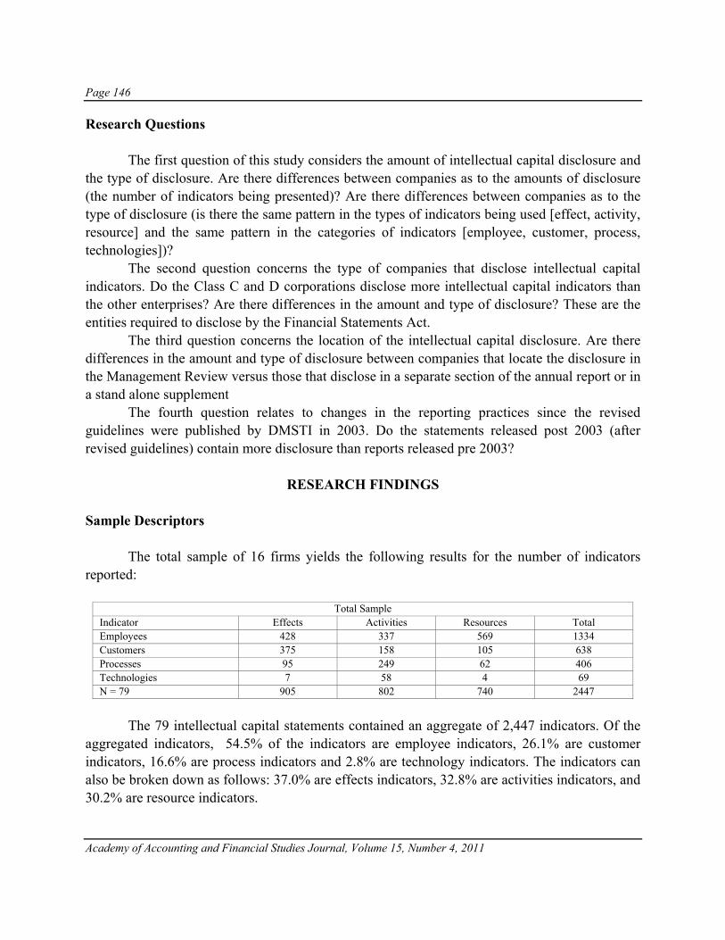
Page 146
Academy of Accounting and Financial Studies Journal, Volume 15, Number 4, 2011
Research Questions
The first question of this study considers the amount of intellectual capital disclosure and the type of disclosure. Are there differences between companies as to the amounts of disclosure (the number of indicators being presented)? Are there differences between companies as to the type of disclosure (is there the same pattern in the types of indicators being used [effect, activity, resource] and the same pattern in the categories of indicators [employee, customer, process, technologies])?
The second question concerns the type of companies that disclose intellectual capital indicators. Do the Class C and D corporations disclose more intellectual capital indicators than the other enterprises? Are there differences in the amount and type of disclosure? These are the entities required to disclose by the Financial Statements Act.
The third question concerns the location of the intellectual capital disclosure. Are there differences in the amount and type of disclosure between companies that locate the disclosure in the Management Review versus those that disclose in a separate section of the annual report or in a stand alone supplement
The fourth question relates to changes in the reporting practices since the revised guidelines were published by DMSTI in 2003. Do the statements released post 2003 (after revised guidelines) contain more disclosure than reports released pre 2003?
RESEARCH FINDINGS Sample Descriptors
The total sample of 16 firms yields the following results for the number of indicators reported:
Total Sample Indicator Effects Activities Resources Total Employees 428 337 569 1334 Customers 375 158 105 638 Processes 95 249 62 406 Technologies 7 58 4 69 N = 79 905 802 740 2447
The 79 intellectual capital statements contained an aggregate of 2,447 indicators. Of the
aggregated indicators, 54.5% of the indicators are employee indicators, 26.1% are customer indicators, 16.6% are process indicators and 2.8% are technology indicators. The indicators can also be broken down as follows: 37.0% are effects indicators, 32.8% are activities indicators, and 30.2% are resource indicators.

Page 147
Academy of Accounting and Financial Studies Journal, Volume 15, Number 4, 2011
The average number of indicators per statement is as follows:
Total Sample Indicator Effects Activities Resources Total Employees 5.42 4.27 7.2 16.89 Customers 4.75 2 1.33 8.08 Processes 1.2 3.15 0.78 5.14 Technologies 0.09 0.73 0.05 0.87 N = 79 11.46 10.15 9.37 30.97
Whiting and Miller (2008) reported on comparative frequencies for categories of
intellectual capital indicators as reported in nine prior studies. All of the studies found that external structure capital attributes have the highest frequency of disclosure. Percentages ranges from a low of 37% to a high of 49%. Internal structure capital attributes ranged from 25–37% while human capital attributes ranged from 10-36%.
Comparative frequency of indicators Indicator Danish Companies Whiting and Miller (2008) Employees (Human capital) 54.50% 10-36% Customers (External structure) 26.10% 37-49% Processes and Technologies (Internal structure) 19.40% 25-37%
The Danish companies in this sample disclose anywhere from 1.5 to 5 times the number
of employee indicators reported by Whiting and Miller (2008). This may be due to the political and economic environment in Denmark and supports a PEA perspective. A number of the companies in the sample have labor representatives serving on the board of directors. At the same time, the number of customer, process and technology indicators disclosed in the sample are less than have been observed in other studies. This may be due to the absence of brand disclosures observed in the Danish sample but present in other studies. Analysis of Questions
The first question asks whether there is consistency in disclosure of indicators amongst companies. This question can be tested using a factorial analysis of variance. Since the number of years that any given company disclosed intellectual capital varied, the average number of indicators for each company was used. Thus, there were 16 observations (one for each company) for the analysis of variance. The variable for equality of number of indicators presented for each company is significant at a level of < .01. The conclusion is the number of indicators disclosed varies amongst companies.
Are there differences in the three types of indicators (effects, activities, and resources) as well as differences between the four categories of indicators (employees, customers, processes, and technology)? The test for equal means of each type of indicator is not significant, the p-value
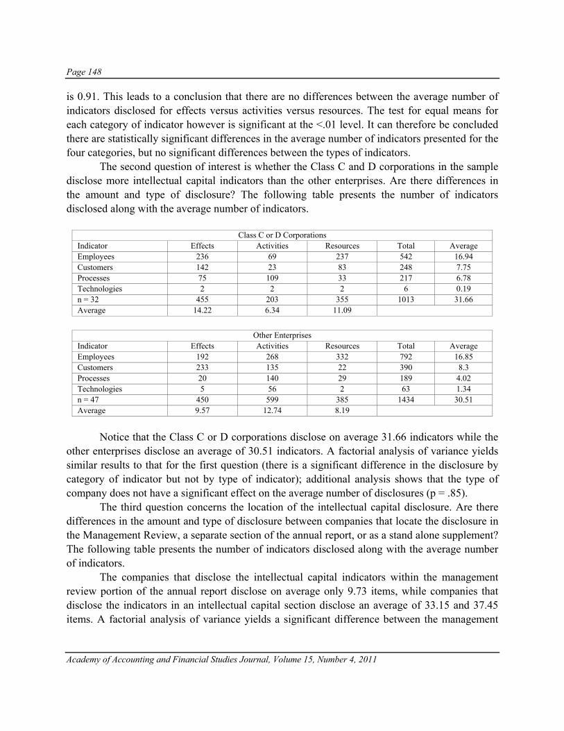
Page 148
Academy of Accounting and Financial Studies Journal, Volume 15, Number 4, 2011
is 0.91. This leads to a conclusion that there are no differences between the average number of indicators disclosed for effects versus activities versus resources. The test for equal means for each category of indicator however is significant at the <.01 level. It can therefore be concluded there are statistically significant differences in the average number of indicators presented for the four categories, but no significant differences between the types of indicators.
The second question of interest is whether the Class C and D corporations in the sample disclose more intellectual capital indicators than the other enterprises. Are there differences in the amount and type of disclosure? The following table presents the number of indicators disclosed along with the average number of indicators.
Class C or D Corporations Indicator Effects Activities Resources Total Average Employees 236 69 237 542 16.94 Customers 142 23 83 248 7.75 Processes 75 109 33 217 6.78 Technologies 2 2 2 6 0.19 n = 32 455 203 355 1013 31.66 Average 14.22 6.34 11.09
Other Enterprises
Indicator Effects Activities Resources Total Average Employees 192 268 332 792 16.85 Customers 233 135 22 390 8.3 Processes 20 140 29 189 4.02 Technologies 5 56 2 63 1.34 n = 47 450 599 385 1434 30.51 Average 9.57 12.74 8.19
Notice that the Class C or D corporations disclose on average 31.66 indicators while the
other enterprises disclose an average of 30.51 indicators. A factorial analysis of variance yields similar results to that for the first question (there is a significant difference in the disclosure by category of indicator but not by type of indicator); additional analysis shows that the type of company does not have a significant effect on the average number of disclosures (p = .85).
The third question concerns the location of the intellectual capital disclosure. Are there differences in the amount and type of disclosure between companies that locate the disclosure in the Management Review, a separate section of the annual report, or as a stand alone supplement? The following table presents the number of indicators disclosed along with the average number of indicators.
The companies that disclose the intellectual capital indicators within the management review portion of the annual report disclose on average only 9.73 items, while companies that disclose the indicators in an intellectual capital section disclose an average of 33.15 and 37.45 items. A factorial analysis of variance yields a significant difference between the management

Page 149
Academy of Accounting and Financial Studies Journal, Volume 15, Number 4, 2011
review disclosers and the section disclosers (p < .001). The difference between the two forms of section disclosers is not significant (p = .19).
Disclosure in Management Review Indicator Effects Activities Resources Total Average Employees 7 0 89 96 8.73 Customers 6 0 0 6 0.55 Processes 0 1 0 1 0.09 Technologies 0 4 0 4 0.36 n = 11 13 5 89 107 9.73 Average 1.18 0.45 8.09
Intellectual Capital Section in Annual Report Indicator Effects Activities Resources Total Average Employees 357 179 327 863 17.98 Customers 309 71 62 442 9.21 Processes 70 150 24 244 5.08 Technologies 7 33 2 42 0.88 n = 48 743 433 415 1591 33.15 Average 15.48 9.02 8.65
Separate Intellectual Capital Report Indicator Effects Activities Resources Total Average Employees 64 158 153 375 18.75 Customers 60 87 43 190 9.5 Processes 25 98 38 161 8.05 Technologies 0 21 2 23 1.15 n = 20 149 364 236 749 37.45 Average 7.45 18.2 11.8
The fourth question addresses whether there are differences in the disclosure of
intellectual capital after the Danish revised guidelines were published in 2003. This can be analyzed by comparing the years 2000-2002 and 2004-2006.
The average number of indicators reported over time has decreased for all categories with the exception of employees/activities, customers/activities, and processes/resources. A factorial analysis of variance was again performed with an additional variable to reflect the pre-2003 and post-2003. Once again, the type of indicator breakdown (effects, activities, resources) was not statistically significant while the category of indicator (employee, customer, process, technology) was significant. The time (pre-2003/post-2003) variable was not statistically significant (p = 0.1985). It can be concluded there are no significant differences in the disclosure of indicators after the revised guidelines were issued.

Page 150
Academy of Accounting and Financial Studies Journal, Volume 15, Number 4, 2011
Averages
2000 - 2002 Indicator Effects Activities Resources Average Employees 6.24 3.84 7.68 17.76 Customers 4.72 1.28 1.64 7.64 Processes 1.36 3.92 0.56 5.84 Technologies 0.2 0.92 0.16 1.28 N = 25 12.52 9.96 10.04 32.52
2004 - 2006 Indicator Effects Activities Resources Average Employees 4.61 4.1 6.71 15.41 Customers 4.34 2.27 1.22 7.83 Processes 0.95 2.34 0.8 4.1 Technologies 0.05 0.66 0 0.71 N = 41 9.95 9.37 8.73 28.05
Change pre 2003 to post 2003 Indicator Effects Activities Resources Average Employees -1.63 0.26 -0.97 -2.35 Customers -0.38 0.99 -0.42 0.19 Processes -0.41 -1.58 0.24 -1.74 Technologies -0.15 -0.26 -0.16 -0.57 -2.39 -0.59 -1.39 -4.37
Analysis of Indicators
The maximum number of indicators for any one company is as follows:
Total Sample N = 79 Indicator Effects Activities Resources Maximum Employees 21 19 10 29 Customers 27 38 18 45 Processes 11 25 8 35 Technologies 5 5 2 11 Maximum 39 79 29 103
This table can be interpreted as follows. The maximum number of employee effects
indicators reported by any of the 16 sample companies was 21, the maximum number of customer activities indicators reported by any of the 16 sample companies was 38, etc. The maximum number of employee indicators reported by any of the 16 sample companies (whether the indicators are an effects indicator, an activities indicator, or a resources indicator) was 29, the maximum customer indicators was 45, etc. The maximum number of effects indicators reported by any of the 16 sample companies (whether the effects indicators are employee, customer, process or technology) was 39, the maximum number of activities indicators was 79, and the maximum number of resources indicators was 29. In aggregate, the maximum total number of

Page 151
Academy of Accounting and Financial Studies Journal, Volume 15, Number 4, 2011
indicators reported of any type had a range of 40 to 103. The minimum number of indicators reported in any given year ranged from 1 to 13 indicators.
Several indicators were consistently reported across companies. All 16 companies disclosed an indicator for number of employees. Nine of the companies disclosed some form of indicator of either employee satisfaction or employee satisfaction with their job. Another nine companies disclosed an indicator for overall customer satisfaction. Five companies disclosed an indicator for the number of customers. Table Three presents a categorization of the specific indicators disclosed.
Table Three Listing of Indicators Employee Indicators
Effects Activities Resources Employee Satisfaction (11) Financial metrics (11) Number of employees (16) Sick days/ Absentee (11) Number in training (10) Seniority (12)
Turnover of staff (11) Training time (4) Age (10) Work conditions (8) Job rotation/ Job sharing (4) Sex (8)
Employee attitudes (8) Work environment (4) New employees (8) Employee Loyalty (5) Conferences (2) Education/ Training
Unsolicited applications (5) Hiring activities (2) Distribution of jobs (5) Ideal employer (4) Job Fairs (1) Experience (4)
Certifications (1) Foreign (3) Work from home (2)
Customer Indicators Effects Activities Resources
Customer Satisfaction (10) Number of …(7) Number of customers (6) Impressions/ Awareness (7) Customer categories (3) Customers: Pareto (3)
Image (3) Activity per employee (3) Turnover (2) Changes in customer base (3) Per employee metrics (2)
Customer Loyalty (2) Size/share (2) Tenure of customer (1)
Process Indicators Effects Activities Resources
Quality (4) Financial metrics (10) Availability (2) On-time delivery (3) Volume of activities (8) Work Environment (2)
Impressions/ Awareness (3) Environment (3) Work networks (1) Utilization (2) Timeliness of activity (2) Type of work (1)
Quality (2) Process documentation (1) Amount of work (1)
Technology Indicators Effects Activities Resources
Satisfaction (1) Financial metrics (3) Skills (1) Portal usage (1) Website activity (3) Technology available (1)
Usage (2) Numbers in parentheses represent the number of companies reporting an indicator
Page 152
Academy of Accounting and Financial Studies Journal, Volume 15, Number 4, 2011
CONCLUSIONS, LIMITATIONS AND FURTHER RESEARCH
The main conclusion of this study is there are differences among the number of indicators and the category of indicators being used in formal intellectual capital reports by Danish companies. The average number of indicators of intellectual capital differs at a statistically significant level as does the relative pattern in the categories (employee, customer, process, technology) of indicators presented. There was not a statistically significant difference in the patterns for the types (effects, activities, resources) of indicators presented. There also was not a significant difference in the number of indicators disclosed by Class C or D corporations versus the other forms of enterprises. There was, however, a significant difference in the location of the disclosure within the annual report. Companies that disclosed intellectual capital as part of the Management Review section of the annual report presented significantly fewer indicators than did the companies that presented disclosure as either an extended note to the report or as a stand-alone intellectual capital statement. Although more disclosure was presented when a stand-alone statement was presented, the difference between that and the extended note was not significant.
There was not a significant difference in the intellectual capital reporting between the two time periods investigated. There was an observed decrease in the indicators disclosed in the time period following the guidelines published by the Danish Ministry of Science, Technology and Innovation in 2003, but the decrease was not statistically significant.
There are a number of limitations to this study. First, the sample is not a random sample of all companies that disclose intellectual capital indicators. Every firm that was identified as disclosing intellectual capital was included in the sample. Second, the sample size is only 16 firms. This limits the power of any statistical tests on the population of reports. Third, the sample was restricted to companies that made their intellectual capital statements available to the general public via the internet.
Further research may include expanding the sample size beyond the 16 firms. An additional question is whether the formal reporting of intellectual capital indicators has any relationship with quantified measures of the value of intellectual capital (for example, see Andriessen, 2004; Ashton, 2005; or Pulic, 2000). Extensions could also be made to relate formal intellectual capital statements and market capitalization (for example, see Abdolmohammadi, 2005). A third extension could be to compare Danish intellectual capital reporting with other countries (for example, the German Federal Ministry of Economics and Labour (Alwert, Bornemann and Kivikas, 2004) has proposed guidelines for intellectual capital reporting by small and medium sized enterprises).

Page 153
Academy of Accounting and Financial Studies Journal, Volume 15, Number 4, 2011
REFERENCES: Abdolmohammadi, M. (2005). Intellectual capital disclosure and market capitalization. Journal of Intellectual
Capital, 6(3), 397-416. Abeysekera, I. (2006). The project of intellectual capital disclosure: Researching the research. Journal of Intellectual
Capital, 7(1) 61-77. Alwert, K., M. Bornemann & M. Kivikas (2004). Intellectual Capital Statement—Made in Germany: Guideline 1.0
on the preparation of an intellectual capital statement. Berlin: Federal Ministry of Economics and Labour. American Institute of Certified Public Accountants (1994). Improving Business Reporting—A Customer Focus:
Meeting the Information Needs of Investors and Creditors, Comprehensive Report of the Special Committee on Financial Reporting (Jenkins Report). New York, NY.
Andriessen, D. (2004). Making Sense of Intellectual Capital: Designing a Method for the Valuation of Intangibles. Burlington. MA: Elsevier Butterworth-Heinemann.
Ashton, R. (2005). Intellectual capital and value creation: a review. Journal of Accounting Literature, 24, 53-134. Bukh, P. (2003). The relevance of intellectual capital disclosure: a paradox? Accounting, Auditing & Accountability
Journal, 16(1), 49-56. Bukh, P., J. Mouritsen, M. Johansen & H. Larsen (2001). Intellectual capital reporting and knowledge management
in Systematic. Kapitel 9 of Videnregnskaber - rapportering og styring af virksomhedens videnressourcer. Copenhagen: Børsens Forlag.
Bukh, P., C. Nielsen, P. Gormsen & J. Mouritsen (2005). Disclosure of information on intellectual capital in Danish IPO prospectuses. Accounting, Auditing & Accountability Journal, 18(6), 713-732.
Danish Act on Commercial Enterprises’ Presentation of Financial Statements, etc. (the Danish Financial Statements Act), Danish Act no. 448 of 7 June 2001
Danish Agency for Trade and Industry (1999). Developing Intellectual Capital Accounts - Experiences from 19 companies. Copenhagen.
Danish Agency for Trade and Industry (2000). A Guideline for Intellectual Capital Statements - A Key to Knowledge Management. Copenhagen.
Danish Ministry of Science, Technology and Innovation (2002). Intellectual Capital Statements in Practice. Copenhagen.
Danish Ministry of Science, Technology and Innovation (2003a). Intellectual Capital Statements—The New Guideline. Copenhagen.
Danish Ministry of Science, Technology and Innovation (2003b). Analysing Intellectual Capital Statements. Copenhagen.
The Danish Trade and Industry Development Council (1997). Intellectual Capital Accounts: Reporting and Managing Intellectual Capital. Copenhagen.
Eccles, R., R, Herz, D. Phillips & E. Keegan (2001). The Value Reporting Revolution: Moving beyond the Earnings Game. New York, NY: Wiley.
Edvinsson, L. & M. Malone (1997). Intellectual Capital: Realizing Your Company’s True Value By Finding Its Hidden Brainpower. New York, NY: Harper Business.
Edvinsson, L. (2002). Corporate Longitude: What You Need To Know To Navigate The Knowledge Economy. London: Financial Times Prentice Hall.
Financial Accounting Standards Board (2001). Improving business reporting: insights into enhancing voluntary disclosures. Norwalk, CT.
Ittner, C. & D. Larcker (1998). Are nonfinancial measures leading indicators of financial performance? An analysis of customer satisfaction. Journal of Accounting Research, 36(Supplement), 1-35.
KPMG (2002). The Danish Financial Statements Act, Copenhagen.

Page 154
Academy of Accounting and Financial Studies Journal, Volume 15, Number 4, 2011
Mouritsen, J., H. Larsen & P. Bukh (2001). Valuing the future: Intellectual capital supplements at Skandia. Accounting, Auditing & Accountability Journal, 14(4), 399-422.
Nielsen, C., P. Bukh, J. Mouritsen, M. Johansen & P. Gormsen (2006). Intellectual capital statements on their way to the stock exchange. Journal of Intellectual Capital, 7(2), 221-240.
Pulic, A (2000). VAICTM—an accounting tool for IC management. International Journal of Technology Management, 20(5-8), 702-714.
Radu, R. (2005). Vision and mission sharing: the Danish intellectual capital statement experience. International Journal of Learning and Intellectual Capital, 2(3), 262-277.
Van der Meer-Kooistra, J. & S. Zijlstra (2001). Reporting on intellectual capital. Accounting, Auditing & Accountability Journal, 14(4), 456-476.
Vergauwen, P. & F. van Alem (2005). Annual report IC disclosures in The Netherlands., France and Germany. Journal of Intellectual Capital, 6(1), 89-104.
Vergauwen, P., L. Bollen & E. Oirbans (2007). Intellectual capital disclosure and intangible value drivers: an empirical study. Management Decision, 45(7), 1163-1180.
Whiting, R. & J. Miller (2008). Voluntary disclosure of intellectual capital in New Zealand annual reports and the ‘Hidden value’. Journal of Human Resource Costing & Accounting, 12(1), 26-50.
Williams, S. (2001). Is intellectual capital performance and disclosure practices related? Journal of Intellectual Capital, 2(3), 192-203.