ACADEMY OF ACCOUNTING AND FINANCIAL STUDIES JOURNAL · ACADEMY OF ACCOUNTING AND FINANCIAL STUDIES...
158
. Volume 15, Special Issue Number 1 Print ISSN: 1096-3685 PDF ISSN: 1528-2635 ACADEMY OF ACCOUNTING AND FINANCIAL STUDIES JOURNAL Mahmut Yardimcioglu Kahramanmaras Sutcu Imam University Editor The Academy of Accounting and Financial Studies Journal is owned and published by the DreamCatchers Group, LLC. Editorial content is under the control of the Allied Academies, Inc., a non-profit association of scholars, whose purpose is to support and encourage research and the sharing and exchange of ideas and insights throughout the world.
Transcript of ACADEMY OF ACCOUNTING AND FINANCIAL STUDIES JOURNAL · ACADEMY OF ACCOUNTING AND FINANCIAL STUDIES...

. Volume 15, Special Issue Number 1 Print ISSN: 1096-3685 PDF ISSN: 1528-2635
ACADEMY OF ACCOUNTING AND FINANCIAL STUDIES JOURNAL
Mahmut Yardimcioglu Kahramanmaras Sutcu Imam University
Editor
The Academy of Accounting and Financial Studies Journal is owned and published by the DreamCatchers Group, LLC. Editorial content is under the control of the Allied Academies, Inc., a non-profit association of scholars, whose purpose is to support and encourage research and the sharing and exchange of ideas and insights throughout the world.

Page ii
Academy of Accounting and Financial Studies Journal, Volume 15, Special Issue Number 1, 2011
Authors execute a publication permission agreement and assume all liabilities. Neither the DreamCatchers Group nor Allied Academies is responsible for the content of the individual manuscripts. Any omissions or errors are the sole responsibility of the authors. The Editorial Board is responsible for the selection of manuscripts for publication from among those submitted for consideration. The Publishers accept final manuscripts in digital form and make adjustments solely for the purposes of pagination and organization.
The Academy of Accounting and Financial Studies Journal is owned and published by the DreamCatchers Group, LLC, PO Box 1708, Arden, NC 28704, USA. Those interested in communicating with the Journal, should contact the Executive Director of the Allied Academies at [email protected].
Copyright 2011 by the DreamCatchers Group, LLC, Arden NC, USA

Page iii
Academy of Accounting and Financial Studies Journal, Volume 15, Special Issue Number 1, 2011
EDITORIAL REVIEW BOARD MEMBERS
Thomas T. Amlie Penn State University-Harrisburg Harrisburg, Pennsylvania
Agu Ananaba Atlanta Metropolitan College Atlanta, Georgia
Manoj Anand Indian Institute of Management Pigdamber, Rau, India
Ali Azad United Arab Emirates University United Arab Emirates
D'Arcy Becker University of Wisconsin - Eau Claire Eau Claire, Wisconsin
Jan Bell Babson College Wellesley, Massachusetts
Roger J. Best Central Missouri State University Warrensburg, Missouri
Linda Bressler University of Houston-Downtown Houston, Texas
Jim Bush Middle Tennessee State University Murfreesboro, Tennessee
Douglass Cagwin Lander University Greenwood, South Carolina
Richard A.L. Caldarola Troy State University Atlanta, Georgia
Eugene Calvasina Southern University and A & M College Baton Rouge, Louisiana
Askar Choudhury Illinois State University Normal, Illinois
Darla F. Chisholm Sam Houston State University Huntsville, Texas
Natalie Tatiana Churyk Northern Illinois University DeKalb, Illinois
Rafik Z. Elias California State University, Los Angeles Los Angeles, California
James W. DiGabriele Montclair State University Upper Montclair, New Jersey
Richard Fern Eastern Kentucky University Richmond, Kentucky
Peter Frischmann Idaho State University Pocatello, Idaho
Farrell Gean Pepperdine University Malibu, California
Luis Gillman Aerospeed Johannesburg, South Africa
Richard B. Griffin The University of Tennessee at Martin Martin, Tennessee
Marek Gruszczynski Warsaw School of Economics Warsaw, Poland
Mohammed Ashraful Haque Texas A&M University-Texarkana Texarkana, Texas

Page iv
Academy of Accounting and Financial Studies Journal, Volume 15, Special Issue Number 1, 2011
EDITORIAL REVIEW BOARD MEMBERS
Mahmoud Haj Grambling State University Grambling, Louisiana
Morsheda Hassan Grambling State University Grambling, Louisiana
Richard T. Henage Utah Valley State College Orem, Utah
Rodger Holland Georgia College & State University Milledgeville, Georgia
Kathy Hsu University of Louisiana at Lafayette Lafayette, Louisiana
Shaio Yan Huang Feng Chia University China
Dawn Mead Hukai University of Wisconsin-River Falls River Falls, Wisconsin
Robyn Hulsart Ohio Dominican University Columbus, Ohio
Evelyn C. Hume Longwood University Farmville, Virginia
Tariq H. Ismail Cairo University Cairo, Egypt
Terrance Jalbert University of Hawaii at Hilo Hilo, Hawaii
Marianne James California State University, Los Angeles Los Angeles, California
Jeff Jewell Lipscomb University Nashville, Tennessee
Jongdae Jin University of Maryland-Eastern Shore Princess Anne, Maryland
Ravi Kamath Cleveland State University Cleveland, Ohio
Desti Kannaiah Middlesex University London-Dubai Campus United Arab Emirates
Marla Kraut University of Idaho Moscow, Idaho
Brian Lee Indiana University Kokomo Kokomo, Indiana
C. Angela Letourneau Winthrop University Rock Hill, South Carolina
Treba Marsh Stephen F. Austin State University Nacogdoches, Texas
Richard Mason University of Nevada, Reno Reno, Nevada
Richard Mautz North Carolina A&T State University Greensboro, North Carolina
Rasheed Mblakpo Lagos State University Lagos, Nigeria
Nancy Meade Seattle Pacific University Seattle, Washington

Page v
Academy of Accounting and Financial Studies Journal, Volume 15, Special Issue Number 1, 2011
EDITORIAL REVIEW BOARD MEMBERS
Christopher Ngassam Virginia State University Petersburg, Virginia
Frank Plewa Idaho State University Pocatello, Idaho
Thomas Pressly Indiana University of Pennsylvania Indiana, Pennsylvania
Hema Rao SUNY-Oswego Oswego, New York
Ida Robinson-Backmon University of Baltimore Baltimore, Maryland
P.N. Saksena Indiana University South Bend South Bend, Indiana
Martha Sale Sam Houston State University Huntsville, Texas
Mukunthan Santhanakrishnan Idaho State University Pocatello, Idaho
Milind Sathye University of Canberra Canberra, Australia
Junaid M. Shaikh Curtin University of Technology Malaysia
Philip Siegel Augusta State University Augusta, Georgia
Mary Tarling Aurora University Aurora, Illinois
Darshan Wadhwa University of Houston-Downtown Houston, Texas
Dan Ward University of Louisiana at Lafayette Lafayette, Louisiana
Suzanne Pinac Ward University of Louisiana at Lafayette Lafayette, Louisiana
Michael Watters Henderson State University Arkadelphia, Arkansas
Clark M. Wheatley Florida International University Miami, Florida
Barry H. Williams King’s College Wilkes-Barre, Pennsylvania
Jan L. Williams University of Baltimore Baltimore, Maryland
Carl N. Wright Virginia State University Petersburg, Virginia

Page vi
Academy of Accounting and Financial Studies Journal, Volume 15, Special Issue Number 1, 2011
TABLE OF CONTENTS
LETTER FROM THE EDITOR ................................................................................................ VIII DO MUTUAL FUND MANAGERS TAKE MORE RISK TOWARD YEAREND?.................. 1
Shuo Chen, State University of New York at Geneseo Anthony Yanxiang Gu, State University of New York at Geneseo Vanthuan Nguyen, Morgan State University John Phelan, University of New Haven
SMALL BUSINESS ENTERPRISES AND TAXATION: A CASE STUDY OF CORPORATE CLIENTS OF A TAX FIRM ............................................................................... 11
Ming Ling Lai, Universiti Teknologi MARA, Malaysia Mazrayahaney Zainal Arifin, Universiti Teknologi MARA, Malaysia
MODELING COST BEHAVIOR: LINEAR MODELS FOR COST STICKINESS .................. 25
Arnel Onesimo O. Uy, De La Salle University THE SECURITIES LITIGATION REFORM AND MARKET REACTIONS TO ANALYST RECOMMENDATION REVISION ......................................................................... 35
Huabing (Barbara) Wang, West Texas A&M University EXCHANGE TRADED NOTES AND THE LEHMAN BANKRUPTCY ................................. 47
Kenneth Washer, Creighton University Randy Jorgensen, Creighton University
MARKET IMPLICATION OF HUMAN CAPITAL INVESTMENT IN TRAINING .............. 59
Chih-Hsien Liao, National Taiwan University Songtao Mo, Purdue University Calumet Julia Grant, Case Western Reserve University

Page vii
Academy of Accounting and Financial Studies Journal, Volume 15, Special Issue Number 1, 2011
INTERNATIONAL PORTFOLIO DIVERSIFICATION BASED ON PARTIAL-CORRELATION .......................................................................................................................... 89
Askar Choudhury, Illinois State University G. N. Naidu, Illinois State University
A CROSS SECTIONAL STUDY OF FINANCIAL MEASURES IN PREDICTING STOCKS’ RISKINESS DURING YEAR 2008 CRASH PERIOD ........................................... 103
Victor Bahhouth, University of North Carolina - Pembroke Ramin Maysami, University of North Carolina - Pembroke
OWNERSHIP STRUCTURE AND FINANCIAL PERFORMANCE IN THE TRUCKING INDUSTRY ........................................................................................................... 111
Arthur J. Francia, University of Houston Mattie C. Porter, University of Houston-Clear Lake Christian K. Sobngwi, University of Houston
A STUDY ON AUDIT PRICING AND MARKET ASSESSMENT OF RISK ........................ 123
Hema Rao, SUNY- Oswego John MacDonald, SUNY- Oswego
LIQUIDITIY AND FINANCIAL LEVERAGE RATIOS: THEIR IMPACT ON COMPLIANCE WITH INTERNATIONAL FINANCIAL REPORTING STANDARDS (IFRS) ................................................................................................................ 135
Rodiel C. Ferrer, De La Salle – Manila, Philippines Glenda J. Ferrer, University of Rizal System, Philippines

Page viii
Academy of Accounting and Financial Studies Journal, Volume 15, Special Issue Number 1, 2011
LETTER FROM THE EDITOR Welcome to the Academy of Accounting and Financial Studies Journal. The editorial content of this journal is under the control of the Allied Academies, Inc., a non profit association of scholars whose purpose is to encourage and support the advancement and exchange of knowledge, understanding and teaching throughout the world. The mission of the AAFSJ is to publish theoretical and empirical research which can advance the literatures of accountancy and finance. As has been the case with the previous issues of the AAFSJ, the articles contained in this volume have been double blind refereed. The acceptance rate for manuscripts in this issue, 25%, conforms to our editorial policies. The Editor works to foster a supportive, mentoring effort on the part of the referees which will result in encouraging and supporting writers. He will continue to welcome different viewpoints because in differences we find learning; in differences we develop understanding; in differences we gain knowledge and in differences we develop the discipline into a more comprehensive, less esoteric, and dynamic metier. Information about the Allied Academies, the AAFSJ, and our other journals is published on our web site. In addition, we keep the web site updated with the latest activities of the organization. Please visit our site and know that we welcome hearing from you at any time. Mahmut Yardimcioglu Kahramanmaras Sutcu Imam University
Page 1
Academy of Accounting and Financial Studies Journal, Volume 15, Special Issue Number 1, 2011
DO MUTUAL FUND MANAGERS TAKE MORE RISK TOWARD YEAREND?
Shuo Chen, State University of New York at Geneseo
Anthony Yanxiang Gu, State University of New York at Geneseo Vanthuan Nguyen, Morgan State University
John Phelan, University of New Haven
ABSTRACT This study finds evidences for both the tournament hypothesis, mutual fund managers who are possible “losers” in the final tournament tend to take greater risk than possible “winners” in the latter part of a year, and the alternative hypothesis, mutual fund managers with higher interim returns are more likely to take greater risk toward the end of the year than those with low interim returns. This behavior aggravates agency problem between mutual fund companies and investors. Results vary with different fund categorizations and over time, which indicate that mutual fund managers’ behavior is inconsistent, and explain why researchers report different findings.
INTRODUCTION Most mutual fund managers receive compensation in proportion of the assets under their management. Unlike hedge funds or pension funds, the mutual fund industry seldom uses rewards based on investment performance (Elton et al., 2003; Golec, 2003). According to Moody’s Manual on Bank and Financial Companies (1996), among 2351 actively managed equity mutual funds, 2190 used asset-based management fees whereas only 39 used performance fees. Thus, mutual fund managers have incentive to attract more new investment inflows because larger assets under their management increase their income. Researchers have found that mutual funds earning the highest returns receive greater increase in new capital (Ippolito, 1992; Sirri & Tufano, 1998). Sirri and Tufano (1998) also find that funds performing poorly do not have a large outflow of capital. This asymmetry between reward and penalty may provide mutual fund managers with an incentive to take greater risk for their funds in order to maximize their own benefits. Since mutual fund managers’ behavior is not directly observable and may conflict with the goal of investors, such excessive risk taking aggravates the agency problem between mutual fund companies and investors. How fund managers adapt their investment behavior to the incentives has been of interest to researchers. One theory views the mutual funds as in a tournament in which the funds outperforming the peers win and receive higher rewards. Brown et al. (1996) argues that
Page 2
Academy of Accounting and Financial Studies Journal, Volume 15, Special Issue Number 1, 2011
investors respond to the annual rankings of funds published by business magazines and services at the end of the calendar year. To win the annual tournament, managers with poor relative year-to-date returns tend to change the risk of their funds before the end of the year. Why would the managers gamble? Grinblatt and Titman (1989) argues that the long-run income of the fund manager is a convex function of his current performance. The gains from outperforming the peers exceed the losses from performing poorly, especially for new managers with smaller assets under management. In this study we apply Arrow’s (1965) theory of risk aversion and utility values to examine the fund managers’ risk-taking behavior. Arrow (1965) advances the hypothesis that the absolute risk aversion is a decreasing function of wealth. He argues that a risky asset is a normal good and the willingness to engage in small bets of fixed size increases with wealth, in the sense that the odds demanded diminish. In other words, risk aversion is decreasing with wealth. This implies that funds with higher year-to-date returns may have stronger incentives to increase risk at the end of the year. The theory of decreasing risk aversion offers the opposite prediction about the relation between risk adjustment and interim returns. The empirical evidence of managers’ risk-changing behavior is mixed in the past studies. Using monthly returns of growth-oriented mutual funds from 1976 to 1991, Brown et al. (1996) find support for the tournament hypothesis that mid-year “losers” tend to increase fund volatility in the latter part of a year more than mid-year “winners.” Similarly, Koski and Pontiff (1999) find a negative relationship between a fund’s performance in the first half of a year and its change in risk in the second half of the year using monthly data. However, Busse (2001) does not find the same behavioral pattern using daily return data. Chevalier and Ellison (1997) finds that funds that perform best have the strongest incentive to gamble, using monthly data of a sample of mutual funds from 1982 to 1992. The goal of this paper is to provide new evidence of fund managers’ risk-adjusting behavior. We test the hypotheses of tournament theory and Arrow’s utility theory using monthly returns of 438 growth-oriented mutual funds over the period of 1990-2000. We analyze the relation between interim performance and fund risk changes using both contingency tables and regression analysis. We use the methodology of Brown et al. (1996) to calculate the variance of returns, where we categorize funds with negative returns as “low return” and positive returns as “high return”. The results indicate that funds with positive interim returns are more likely to increase risk at the end of the year than funds with negative returns. The results are consistent with the prediction of Arrow’s theory. We also relate risk adjustment to interim fund performance in a multivariate analysis. The pooled regression results lend support to the theory of risk aversion and utilities values as risk adjustment and interim returns are positively related. The organization of the paper is as follows. Section 2 discusses the hypotheses that lay foundation for our empirical analysis. Section 3 describes the data and methodology. Section 4 presents results of the contingency tables and regression analysis, and section 5 concludes.
Page 3
Academy of Accounting and Financial Studies Journal, Volume 15, Special Issue Number 1, 2011
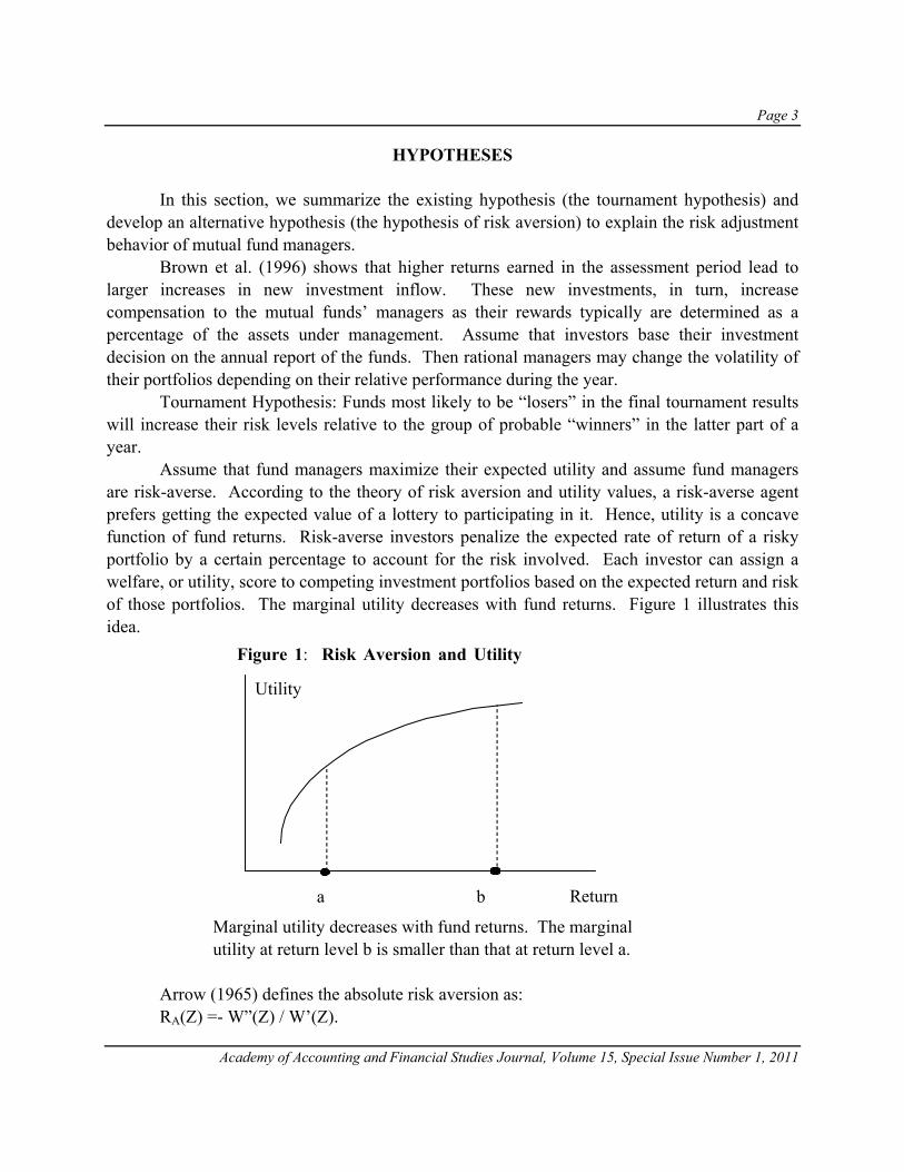
HYPOTHESES In this section, we summarize the existing hypothesis (the tournament hypothesis) and develop an alternative hypothesis (the hypothesis of risk aversion) to explain the risk adjustment behavior of mutual fund managers. Brown et al. (1996) shows that higher returns earned in the assessment period lead to larger increases in new investment inflow. These new investments, in turn, increase compensation to the mutual funds’ managers as their rewards typically are determined as a percentage of the assets under management. Assume that investors base their investment decision on the annual report of the funds. Then rational managers may change the volatility of their portfolios depending on their relative performance during the year. Tournament Hypothesis: Funds most likely to be “losers” in the final tournament results will increase their risk levels relative to the group of probable “winners” in the latter part of a year. Assume that fund managers maximize their expected utility and assume fund managers are risk-averse. According to the theory of risk aversion and utility values, a risk-averse agent prefers getting the expected value of a lottery to participating in it. Hence, utility is a concave function of fund returns. Risk-averse investors penalize the expected rate of return of a risky portfolio by a certain percentage to account for the risk involved. Each investor can assign a welfare, or utility, score to competing investment portfolios based on the expected return and risk of those portfolios. The marginal utility decreases with fund returns. Figure 1 illustrates this idea.
Marginal utility decreases with fund returns. The marginal utility at return level b is smaller than that at return level a.
Arrow (1965) defines the absolute risk aversion as: RA(Z) =- W”(Z) / W’(Z).
Figure 1: Risk Aversion and Utility
Return
Utility
a b
Page 4
Academy of Accounting and Financial Studies Journal, Volume 15, Special Issue Number 1, 2011
Where W(Z) is the utility function and W’(Z) and W”(Z) are the first and second derivative of the utility function. Arrow advances the hypothesis that RA(Z) is a decreasing function of Z, where Z refers to final wealth at the end of the period for which the investment decision is binding. This implies that when wealth is larger, the willingness to take risks of fixed size will be larger. In other words, risk aversion decreases as wealth increases. Fund managers with higher interim returns also expect higher returns at the end of the year. The theory of risk aversion implies that fund managers with higher interim returns may be more willing to take risks than fund managers with low interim returns. Hypothesis of Decreasing Risk Aversion: Fund managers with higher interim returns are more likely to increase risk at the end of the year than fund managers with low interim returns.
DATA AND METHODOLOGY The data for this paper consists of monthly returns for 438 growth-oriented mutual funds contained in 2002 Morningstar Database. We restrict our analysis to funds which is categorized as either “growth” or “growth and income” in the prospectus objective, or “growth” in the Morningstar category. We select this category of funds because they are the most widely followed and ranked, and are likely to have risk-taking tendency (Brown et al., 1996; McDonald, 1974). For each fund in the sample, monthly return data are available from January 1990 to December 2000. The sample excludes new entrants after December 1989. It also excludes funds with unavailable return data. Table 1 reports a summary statistics of our sample.
Table 1: Descriptive Statistics for a sample of 438 Mutual Funds, 1990-2000 This table shows the monthly return statistics of the mutual fund sample by subgroups. The data are taken from the 2002 Morningstar Database. The study period is from January 1990 to December 2000. The funds either have a “growth” or “growth and income” in the prospectus objective, or have a “growth” in the Morningstar category. New entrants after December 1989, and funds with unavailable data are excluded.
Fund Group No. of Funds Mean Monthly Return All 438 1.29% Growth 244 1.27% Growth and Income 123 1.12% Small Company 37 1.45% Aggressive Growth 28 1.30% Others 6 1.33%
We first adopt the method of Brown et al. (1996) to construct two variables, returns (RTN) and risk (RAR). Brown et al. (1996) find that every interim period ending from May to August generates significant test results, while Chevalier and Ellison (1997) use the assessment period ending in September in the analysis. We pick August as the division point to break the year into two periods, the first 8 months and the last 4 months.. RTN is the compound total
Page 5
Academy of Accounting and Financial Studies Journal, Volume 15, Special Issue Number 1, 2011
return through the first 8 months of one calendar year. RTN helps to measure whether a fund is performing relatively well or poorly at the end of August. RTNjy = [(1+rjy1) (1+rjy2) …(1+rjy8)] – 1, (1) where RTNjy stands for compound total return for fund j in the first eight months of year y and rjy1 is return for fund j in year y and month 1. RAR is the ratio of standard deviation of return in the last 4 months (SD2) to standard deviation of return in the first 8 months (SD1) of each year. RAR measures whether a fund changes its risk in the latter part of a year. RARjy = SD2jy / SD1jy , (2) where
7)(
18
12
)81(∑ = −−= m jyjym
jy
rrSD
, 3)(
212
92
)129(∑ = −−= m jyjym
jy
rrSD
. The two standard deviations are computed relative to the mean return over the corresponding sub-period. According to the hypothesis of risk aversion, this ratio should be significantly larger for funds that performed well at mid-year than for funds that performed poorly. We create a (RTN, RAR) pair for every fund in each year between 1990 and 2000, where RTN is the compound return in the first eight months and RAR is the standard deviation in the last four months. We classify a RAR that is above the median RAR value as “high”, and below the median value as “low.” Also, we classify a RTN that is above the median RTN value as “high”, and below the median value as “low.” We also try an alternative way to categorize RTN’s. We classify a RTN as “low” if it is negative and “high” if it is positive. We do this because investors tend to identify a fund as “loser” if the fund’s return is negative while other funds’ returns are positive. We still categorize RAR by median. We construct a two-by-two contingency table in which we put each fund into one of four cells: (high RTN, high RAR), (high RTN, low RAR), (low RTN, high RAR), and (low RTN, low RAR). We count the number of funds in each of the four cells aggregating over 11 years. If we classify RTN’s by median, the percentage of funds in each cell should be 25% if there are no differences in risk among those funds. Hence, the null hypothesis is that the percentage of all observations falling into each of the four cells is the same, i.e. equals to 0.25. In the above analysis we measure the total risk of each fund by standard deviation. We next measure the systematic risk by calculating the beta of each fund relative to the entire sample. We examine the hypotheses with regressions similar to those in Koski and Pontiff (1999) and Busse (2001).
Page 6
Academy of Accounting and Financial Studies Journal, Volume 15, Special Issue Number 1, 2011
To test the relation between prior fund performance and risk adjustment, we estimate the following equation: BETAjy2 - BETAjy1 = α + γPERFjy1 + φBETAjy1 + εjy , (3) where PERFjy1 is the difference between the compound return of the fund and the average of compound returns of all funds in the sample during the first eight months of the year. BETAjy2 and BETAjy1 are the estimates of risk for fund j in two sub-periods within one year. We calculate these two variables by running two time-series regressions for each fund in each year, one from January through August, and the other from September through December: Rjym = αjy1+ βjy1 RMym + εjym , m = 1 to 8, Rjym = αjy2+ βjy2 RMym + εjym , m = 9 to 12, (4) where RMym is the return of the Standard and Poor’s 500 Index in year y and month m , and Rjym is the return of fund j in year y and month m.
EMPIRICAL RESULTS We first report the contingency tables. Table 2 shows cell frequencies for two different designs
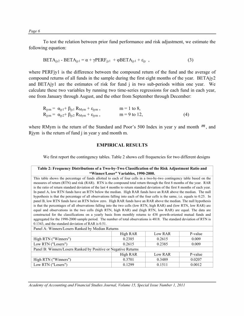
Table 2: Frequency Distributions of a Two-by-Two Classification of the Risk Adjustment Ratio and “Winner/Loser” Variables, 1990-2000.
This table shows the percentage of funds allotted to each of four cells in a two-by-two contingency table based on the measures of return (RTN) and risk (RAR). RTN is the compound total return through the first 8 months of the year. RAR is the ratio of return standard deviation of the last 4 months to return standard deviation of the first 8 months of each year. In panel A, low RTN funds have an RTN below the median. High RAR funds have an RAR above the median. The null hypothesis is that the percentage of all observations falling into each of the four cells is the same, i.e. equals to 0.25. In panel B, low RTN funds have an RTN below zero. High RAR funds have an RAR above the median. The null hypothesis is that the percentages of all observations falling into the two cells (low RTN, high RAR) and (low RTN, low RAR) are equal and observations in the two cells (high RTN, high RAR) and (high RTN, low RAR) are equal. The data are constructed for the classifications on a yearly basis from monthly returns to 438 growth-oriented mutual funds and aggregated for the 1990-2000 sample period. The number of total observations is 4818. The standard deviation of RTN is 0.1343, and the standard deviation of RAR is 0.51. Panel A: Winners/Losers Ranked by Median Returns High RAR Low RAR P-value High RTN ("Winners") 0.2385 0.2615 0.009 Low RTN ("Losers") 0.2615 0.2385 0.009 Panel B: Winners/Losers Ranked by Positive or Negative Returns High RAR Low RAR P-value High RTN ("Winners") 0.3701 0.3489 0.0207 Low RTN ("Losers") 0.1299 0.1511 0.0012
Page 7
Academy of Accounting and Financial Studies Journal, Volume 15, Special Issue Number 1, 2011
Panel A of Table 2 lists results for winners and losers categorized by the median value of RTN. We find that the frequency in the cell (low RTN, high RAR) is significantly higher than 0.25 (P-value = 0.009). This is consistent with the tournament hypothesis. Panel B of Table 2 lists results for winners and losers categorized by positive or negative RTN. The frequency in the cell (high RTN, high RAR) is significantly higher than that in the cell (high RTN, low RAR), indicating that funds earning interim positive returns may increase their risks toward the end of the year. The frequency in the cell (low RTN, high RAR) is significantly lower than that in the cell (low RTN, low RAR). This indicates that the interim “losers” do not necessarily increase their risks in the last few months of a year.
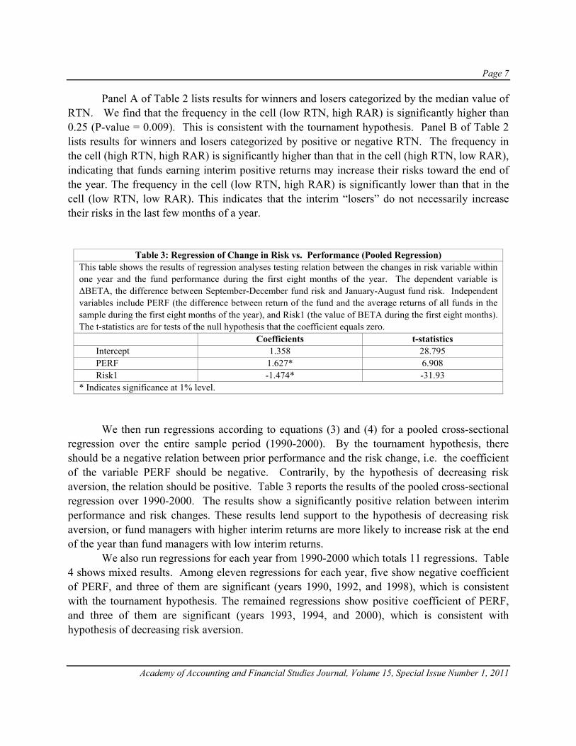
Table 3: Regression of Change in Risk vs. Performance (Pooled Regression) This table shows the results of regression analyses testing relation between the changes in risk variable within one year and the fund performance during the first eight months of the year. The dependent variable is ΔBETA, the difference between September-December fund risk and January-August fund risk. Independent variables include PERF (the difference between return of the fund and the average returns of all funds in the sample during the first eight months of the year), and Risk1 (the value of BETA during the first eight months). The t-statistics are for tests of the null hypothesis that the coefficient equals zero. Coefficients t-statistics
Intercept 1.358 28.795 PERF 1.627* 6.908 Risk1 -1.474* -31.93
* Indicates significance at 1% level. We then run regressions according to equations (3) and (4) for a pooled cross-sectional regression over the entire sample period (1990-2000). By the tournament hypothesis, there should be a negative relation between prior performance and the risk change, i.e. the coefficient of the variable PERF should be negative. Contrarily, by the hypothesis of decreasing risk aversion, the relation should be positive. Table 3 reports the results of the pooled cross-sectional regression over 1990-2000. The results show a significantly positive relation between interim performance and risk changes. These results lend support to the hypothesis of decreasing risk aversion, or fund managers with higher interim returns are more likely to increase risk at the end of the year than fund managers with low interim returns. We also run regressions for each year from 1990-2000 which totals 11 regressions. Table 4 shows mixed results. Among eleven regressions for each year, five show negative coefficient of PERF, and three of them are significant (years 1990, 1992, and 1998), which is consistent with the tournament hypothesis. The remained regressions show positive coefficient of PERF, and three of them are significant (years 1993, 1994, and 2000), which is consistent with hypothesis of decreasing risk aversion.

Page 8
Academy of Accounting and Financial Studies Journal, Volume 15, Special Issue Number 1, 2011
Table 4: Regression of Change in Risk vs. Performance (Year by Year)
This table shows the results of regression analyses testing relation between the changes in risk variable within one year and the fund performance during the first eight months of the year. The dependent variable is ΔBETA, the difference between September-December fund risk and January-August fund risk. Independent variables include PERF (the difference between return of the fund and the average returns of all funds in the sample during the first eight months of the year), and Risk1 (the value of BETA during the first eight months). The t-statistics (in parentheses) are for tests of the null hypothesis that the coefficient equals zero.
Sample period Intercept PERF Risk1 1990 0.189 -2.235* 0.03
(2.347) (-4.704) (0.384) 1991 0.363 -0.093 -0.477*
(6.00) (-0.558) (-8.722) 1992 1.458 -2.813* -1.403*
(14.105) (-4.434) (-9.509) 1993 1.121 1.348* -1.126*
(11.350) (2.734) (-13.731) 1994 0.376 1.221* -0.554*
(5.421) (3.139) (-7.708) 1995 1.15 0.311 -1.080*
(23.071) (0.771) (-17.377) 1996 0.891 0.034 -1.131*
(14.328) (0.070) (-24.403) 1997 0.631 -0.38 -0.607*
(9.765) (-1.510) (-7.938) 1998 7.548 -4.673* -7.952*
(11.538) (-3.242) (-13.770) 1999 0.256 0.287 -0.275*
(3.021) (0.951) (-3.289) 2000 1.924 1.824* -1.763*
(21.242) (5.328) (-15.572) * Indicates significance at 1% level.
CONCLUSION
In this study we examine the monthly returns of 438 growth-oriented mutual funds over the period of 1990-2000 and reveal some phenomena of the risk adjustment behavior of mutual fund managers. Results of the study vary with different fund categorizations. They are consistent with the tournament hypothesis when we categorize the funds by median values of interim return and risk adjustment ratio. However, the results support the hypothesis of decreasing risk aversion if we categorize the funds by positive or negative interim returns. The significantly positive relation between risk adjustment and interim returns indicates that fund managers with higher interim returns are more likely to increase risk at the end of the year than fund managers with

Page 9
Academy of Accounting and Financial Studies Journal, Volume 15, Special Issue Number 1, 2011
low interim returns. Furthermore, when running regression for each year separately, we find a significantly negative relation between interim performance and risk change for 3 annual periods and a significantly positive relation for another 3 annual periods. These results may indicate variations in mutual fund managers’ behavior, and may explain why researchers have reported conflicting evidences, i.e., they used different categorization and time periods of the data in their studies. Further research is needed in order to reveal the complex risk-taking behavior of mutual fund managers.
REFERENCES Arrow, K. (1965). Aspects of the theory of risk-bearing. (Helsinki). Brown, K., W. Harlow & L. Starks (1996). Of tournaments and temptations: an analysis of managerial incentives in
the mutual fund industry. Journal of Finance 51, 85-110. Busse, J. (2001). Another look at mutual fund tournaments. Journal of Financial and Quantitative Analysis 36, 53-
73. Chevalier, J. & G. Ellison (1997). Risk taking by mutual funds as a response to incentives. Journal of Political
Economy 105, 1167-1200. Elton, E.J., M. J. Gruber, & C. R. Blake (2003). Incentive fees and mutual funds. Journal of Finance 58, 779-804. Golec, J. (2003). Regulation and the rise in asset-based mutual fund management fees. Journal of Financial Research
26, 19-30. Grinblatt M. & S. Titman (1989). Adverse risk incentives and the design of performance-based contracts.
Management Science 35, 807-822. Ippolito, R. (1992). Consumer reaction to measures of poor quality: evidence from the mutual fund industry. Journal
of Law and Economics 35, 45-70. Koski, J. & J. Pontiff (1999). How are derivatives used? Evidence from the mutual fund industry. Journal of
Finance 54, 791-816. McDonald, J. (1974). Objectives and performance of mutual funds, 1960-1969. Journal of Financial and
Quantitative Analysis 9, 311-333. Sirri, E. & P. Tufano (1998). Costly search and mutual fund flows. Journal of Finance 53, 1589-1622.

Page 10
Academy of Accounting and Financial Studies Journal, Volume 15, Special Issue Number 1, 2011
Page 11
Academy of Accounting and Financial Studies Journal, Volume 15, Special Issue Number 1, 2011
SMALL BUSINESS ENTERPRISES AND TAXATION: A CASE STUDY OF CORPORATE CLIENTS OF A TAX
FIRM
Ming Ling Lai, Universiti Teknologi MARA, Malaysia Mazrayahaney Zainal Arifin, Universiti Teknologi MARA, Malaysia
ABSTRACT
This study aims to find out tax compliance complexities faced by small to medium-sized enterprises (SMEs) in the era of self-assessment tax system. A survey was used to collect data. SMEs with a paid-up share capital not exceeding RM2.5 million were sampled. In the month of August 2008, 200 questionnaires were posted to corporate clients of tax firm in Malaysia. A total of 127 usable responses were received. The effective response rate was 63.5%. This study uncovered that not all SMEs surveyed have fully computerised their accounting system. Most SMEs have difficulties in estimating tax payable, remembering tax deadlines, understanding taxation laws and complying with them. The issuances of Public Rulings are not helping SMEs to better understand the taxation laws. The respondents indicated that the tax authorities delayed in the tax refund process and slow in responding to tax correspondence. The SMEs also suffered additional compliance costs in terms of time spent and tax agent’s fees. This study provides important insights on tax compliance complexities facing the SMEs in the business world. The findings suggest that the tax authorities to develop a simplified tax system for SMEs to lighten their tax compliance burden in the midst of economic downturn. Scholarly study on SMEs and taxation is scant; hence, this paper contributes to fill up a knowledge gap. Keywords: Malaysia, self-assessment, small to medium sized enterprises, taxation, tax compliance, tax system.
INTRODUCTION Worldwide and in Malaysia, small to medium sized enterprises (SMEs) play a pivotal role in a country’s economic development. Besides creating job opportunity, SMEs contribute substantially to the growth and development of a nation. In SME Annual Report 2006, it was reported that Malaysian SMEs generated 32% of the country’s Gross Domestic Product and 19% of exports (Central Bank of Malaysia, 2007). However, to be viable in business, SMEs face huge challenges. SMEs need to meet a host of regulatory obligations, such as licensing requirements, employment regulations, workers’ compensation and tax compliance obligations among others.
Page 12
Academy of Accounting and Financial Studies Journal, Volume 15, Special Issue Number 1, 2011
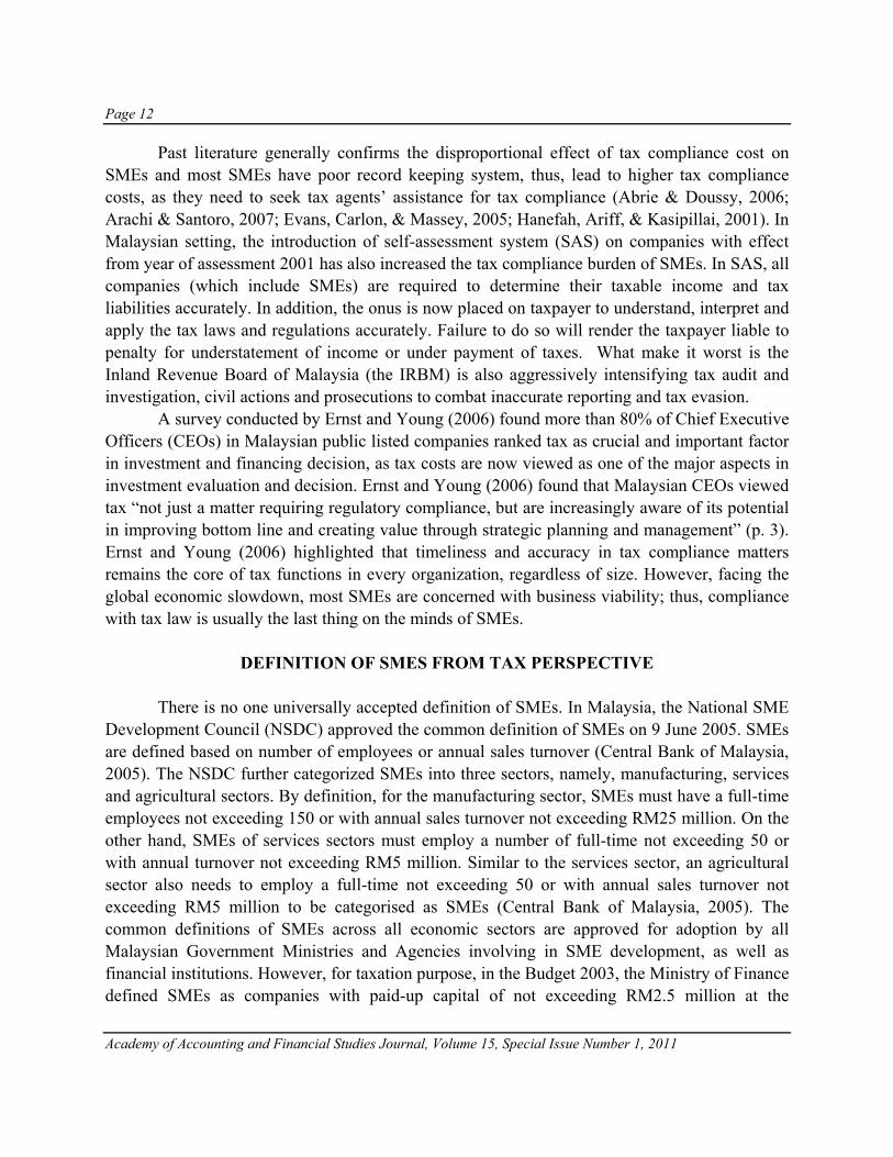
Past literature generally confirms the disproportional effect of tax compliance cost on SMEs and most SMEs have poor record keeping system, thus, lead to higher tax compliance costs, as they need to seek tax agents’ assistance for tax compliance (Abrie & Doussy, 2006; Arachi & Santoro, 2007; Evans, Carlon, & Massey, 2005; Hanefah, Ariff, & Kasipillai, 2001). In Malaysian setting, the introduction of self-assessment system (SAS) on companies with effect from year of assessment 2001 has also increased the tax compliance burden of SMEs. In SAS, all companies (which include SMEs) are required to determine their taxable income and tax liabilities accurately. In addition, the onus is now placed on taxpayer to understand, interpret and apply the tax laws and regulations accurately. Failure to do so will render the taxpayer liable to penalty for understatement of income or under payment of taxes. What make it worst is the Inland Revenue Board of Malaysia (the IRBM) is also aggressively intensifying tax audit and investigation, civil actions and prosecutions to combat inaccurate reporting and tax evasion. A survey conducted by Ernst and Young (2006) found more than 80% of Chief Executive Officers (CEOs) in Malaysian public listed companies ranked tax as crucial and important factor in investment and financing decision, as tax costs are now viewed as one of the major aspects in investment evaluation and decision. Ernst and Young (2006) found that Malaysian CEOs viewed tax “not just a matter requiring regulatory compliance, but are increasingly aware of its potential in improving bottom line and creating value through strategic planning and management” (p. 3). Ernst and Young (2006) highlighted that timeliness and accuracy in tax compliance matters remains the core of tax functions in every organization, regardless of size. However, facing the global economic slowdown, most SMEs are concerned with business viability; thus, compliance with tax law is usually the last thing on the minds of SMEs.
DEFINITION OF SMES FROM TAX PERSPECTIVE There is no one universally accepted definition of SMEs. In Malaysia, the National SME Development Council (NSDC) approved the common definition of SMEs on 9 June 2005. SMEs are defined based on number of employees or annual sales turnover (Central Bank of Malaysia, 2005). The NSDC further categorized SMEs into three sectors, namely, manufacturing, services and agricultural sectors. By definition, for the manufacturing sector, SMEs must have a full-time employees not exceeding 150 or with annual sales turnover not exceeding RM25 million. On the other hand, SMEs of services sectors must employ a number of full-time not exceeding 50 or with annual turnover not exceeding RM5 million. Similar to the services sector, an agricultural sector also needs to employ a full-time not exceeding 50 or with annual sales turnover not exceeding RM5 million to be categorised as SMEs (Central Bank of Malaysia, 2005). The common definitions of SMEs across all economic sectors are approved for adoption by all Malaysian Government Ministries and Agencies involving in SME development, as well as financial institutions. However, for taxation purpose, in the Budget 2003, the Ministry of Finance defined SMEs as companies with paid-up capital of not exceeding RM2.5 million at the

Page 13
Academy of Accounting and Financial Studies Journal, Volume 15, Special Issue Number 1, 2011
beginning of the basis period. As this study is about SMEs and taxation, hence, SMEs are defined as companies that have paid-up share capital not exceeding RM2.5 million at the beginning of the basis period.
KEY TAXES AFFECTING MALAYSIAN SMES Generally, Malaysian SMEs exist in different legal forms such as sole proprietorship, partnerships and private limited companies. They are generally subject to the following taxes:
Income tax on income derived from Malaysia or received in Malaysia from outside Malaysia. In year of assessment (YA) 2007, on the first chargeable income of RM500,000, the tax rate is 20%. In turn, chargeable income exceeds RM500,000 will be charged at 27% (Note that this rate has been reduced to 26% and 25% in YA 2008 and YA2009 respectively)
Sales tax on supplies of goods made in Malaysia, and importation of goods into Malaysia. Manufacturers of taxable goods can claim a credit for the sales tax paid on input, but need to charge and account for sales tax on their output in every 2 calendar months. The general tax rate is 10%.
Services tax on provision of taxable service in Malaysia. Businesses that reached the threshold limit need to register to be a taxable person, then charge and account for service tax in every two calendar months. Currently, the standard service tax rate is 5%.
IMPLICATIONS OF SELF-ASSESSMENT TAX SYSTEM ON MALAYSIAN SMES
The introduction of self-assessment system effective from year of assessment 2001 has initiated the need for new companies to estimate their tax payable and pay monthly instalment upon commencement. New companies are required to submit tax estimates within 3 months from the date of commencement of operations with instalment payments commencing from the sixth month of the basis period. However, in Budget 2008, it was proposed that SMEs (those companies with paid up share capital not more than 2.5 million at the beginning of the basis period) will be exempted from submitting estimate of tax payable and instalment payments for the first two years of assessment after commencement of business operation. On the other hand, all existing companies are required to submit estimates of tax payable not later than 30 days before the beginning of the basis period. Nonetheless, with effect from year of assessment 2003, a company may revise the estimate of income tax payable in a ‘prescribed form’ (CP204A) in the sixth month, or the ninth month or in both the months of the basis period for a year of assessment. The law also stated that the estimated tax payable for the current year of assessment must not less than 85% from the estimated or revised estimated tax payable of immediate preceding year. Meanwhile, the monthly instalment payment will due on the 10th of every month commencing from the second month of the basis period of the year of

Page 14
Academy of Accounting and Financial Studies Journal, Volume 15, Special Issue Number 1, 2011
assessment. Failure to pay tax instalment on time will subject to a 10% penalty on the amount unpaid, by virtue of section 107C (9) of the Income Tax Act, 1967. In addition, a 10% + 5% penalty will also be imposed for every late payment of balance of tax payable. On top of that, if the actual assessment exceeds the original estimate or revised estimate by the amount exceeding 30% of the actual tax payable, the difference will be subject to a penalty of 10%. In respect of the deadline to file tax return form, SMEs (sole proprietors or partners) must submit tax return form by 30 June every year. Whilst, SMEs (private limited companies) must submit tax return within 7 months after the companies closed its accounts. Failure to furnish a tax return on time, with prosecution, the fine is between RM200 to RM2,000 or six months’ imprisonment or both, as stated in Section 112 (1) of the Income Tax Act, 1967.
SMES, TAX COMPLIANCE AND COSTS OF TAX COMPLIANCE Abrie and Doussy (2006) found that out of seven tax incentives offered by the government of South Africa to SMEs, only three incentives were known to the SMEs in that country. More than half of the African SMEs surveyed were not aware of the other four incentives available to them. These scenarios indicated that the African tax system was too complicated at the time of study, and SMEs lacked tax skills and tax campaigns were not successful done. In Malaysia, several tax incentives are outlined in the Income Tax Act (1967) and Promotion of Investment Act (1986), for example pioneer status tax exemption, investment tax allowances, reinvestment allowance, exemptions, specific deduction and double deduction are purposefully designed for the Malaysian SMEs. No official statistics to show if SMEs are aware of the existence of the relevant incentives and exemptions that the government has provided to reduce their tax burden. However, what is clear is, in order for SMEs to take advantage of these tax incentives and exemptions, SMEs need to have adequate tax knowledge to deploy appropriate tax planning strategies to utilise the tax incentive fully. Past studies found most SMEs (the sole owners, partners) are not tax literate; it was found that SMEs lack sufficient knowledge on how to compute tax liability and to claim the relevant tax incentives in Malaysia (Hanefah et al., 2001) and in Australia (Evans et al., 2005). Indeed, understanding the taxation laws may be a burden to the SMEs, what more fully complying with it. A simple yearly requirement such as estimating a tax payable is difficult to the SMEs as they could not forecast their business prospects. On top of this, there are many tax deadlines to be remembered, and from time to time, tax policies are subjected to changes and revision. Consequentially, to be tax complaint, most SMEs seek tax agents to help them to compute tax liability and to file tax return. However, tax agents’ service is costly and ironically, at present, the fees paid to tax agents is not deductible. Hence, tax agent’s fee increase tax compliance cost. Several studies had attempted to study tax compliance costs of SMEs in Malaysia (Abdul-Jabbar & Pope, 2008; Hanefah et al., 2001). Hanefah et al. (2001) examined initial

Page 15
Academy of Accounting and Financial Studies Journal, Volume 15, Special Issue Number 1, 2011
compliance costs of SMEs in addition to the regular compliance costs. As self-assessment system requires taxpayers to keep appropriate records and to exercise reasonable care in the reporting and submission of tax returns. They found SMEs need to incur initial compliance costs, that is cost relating to the implementation of new tax laws and costs linked with the learning process. A big amount of initial compliance costs may be required in preparing for the new tax system, and SMEs need to incur costs when major changes are made to the self-assessment system in stages. Hanefah, et al. (2001) defined compliance costs to “numbers of hours spent in preparing tax returns, administrative expenses, and any money spent on the procurement of the services of tax professionals” (p. 78). In general, compliance costs can be categorised into internal and external costs. Internal costs are time spent by company staff in order to maintain and prepare tax information for their professional advisers, completing and perusing completed tax forms liaising with income tax officers on matters pertaining inquiries, objections to tax assessment and appeals. On the other hand, external costs comprised of payments made to acquire the services from professional advisers outside a company; such as the lawyer, accountants, investment advisers and tax representative. Basically, external costs are much more easier be recognised compared to the internal costs. Besides compliance costs, computational costs occur from compiling and maintaining relevant information required by the income tax officers. This cost is an unavoidable cost for SMEs when being selected for tax audit or under tax investigation (Abdul-Jabbar & Pope, 2008). Meanwhile, tax planning costs are related to the tax minimising efforts of a company to manage its tax-related matters. In contrary to computational costs, tax planning costs are avoidable as the costs will only arise if the management decide to use tax planning strategies to mitigate and legally avoid paying taxes.
SMES AND TAX CORRESPONDENCE In Africa, from 15 September 2006 to 5 January 2007, Foreign Investment Advisory Service (FIAS) conducted a study to find out tax compliance burden for small businesses. FIAS(2007) found that the South African Revenue Service’s (SARS) commitment to respond to all correspondence is below expectation. FIAS (2007) found the SARS “over promised, under delivered”. The SARS’ service centre promised to inform the taxpayers of possible reasons of why the reply could not be made promptly and when the taxpayers should expected to receive the said reply. However, in practice, the taxpayers were not actually informed. Meanwhile, in Malaysia, before the implementation of SAS, many taxpayers found that the IRBM’s officers were slow in responding to tax correspondence, especially with regard to tax refund. Several taxpayers complained that they had made various phone calls and written letters after letters to get tax refund; unfortunately, not only tax refund was not received, no written reply was given by the IRBM (Bulbir, 2003; Lee, 1997; Puran, 1997). Besides tax refund matter, there were incidences that the IRBM also slow in responding to tax appeal cases (Concern Taxpayer, 1997).
Page 16
Academy of Accounting and Financial Studies Journal, Volume 15, Special Issue Number 1, 2011
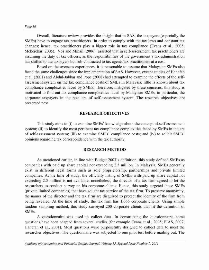
Overall, literature review provides the insight that in SAS, the taxpayers (especially the SMEs) have to engage tax practitioners in order to comply with the tax laws and constant tax changes; hence, tax practitioners play a bigger role in tax compliance (Evans et al., 2005; Mckerchar, 2005). Vos and Mihail (2006) asserted that in self-assessment, tax practitioners are assuming the duty of tax officers, as the responsibilities of the government’s tax administration has shifted to the taxpayers but sub-contracted to tax agents/tax practitioners at a cost. Based on the overseas experiences, it is reasonable to assume that Malaysian SMEs also faced the same challenges since the implementation of SAS. However, except studies of Hanefah et al. (2001) and Abdul-Jabbar and Pope (2008) had attempted to examine the effects of the self-assessment system on the tax compliance costs of SMEs in Malaysia, little is known about tax compliance complexities faced by SMEs. Therefore, instigated by these concerns, this study is motivated to find out tax compliance complexities faced by Malaysian SMEs, in particular, the corporate taxpayers in the post era of self-assessment system. The research objectives are presented next.
RESEARCH OBJECTIVES This study aims to (i) to examine SMEs’ knowledge about the concept of self-assessment system; (ii) to identify the most pertinent tax compliance complexities faced by SMEs in the era of self-assessment system; (iii) to examine SMEs’ compliance costs; and (iv) to solicit SMEs’ opinions regarding tax correspondence with the tax authority.
RESEARCH METHOD As mentioned earlier, in line with Budget 2003’s definition, this study defined SMEs as companies with paid up share capital not exceeding 2.5 million. In Malaysia, SMEs generally exist in different legal forms such as sole proprietorship, partnerships and private limited companies. At the time of study, the officially listing of SMEs with paid up share capital not exceeding 2.5 million is not available, nonetheless, the director of a tax firm agreed to let the researchers to conduct survey on his corporate clients. Hence, this study targeted those SMEs (private limited companies) that have sought tax service of the tax firm. To preserve anonymity, the names of the director and the tax firm are disguised to protect the identity of the firm from being revealed. At the time of study, the tax firm has 1,066 corporate clients. Using simple random sampling method, this study surveyed 200 corporate clients that fit the definition of SMEs. A questionnaire was used to collect data. In constructing the questionnaire, some questions have been adapted from several studies (for example Evans et al., 2005; FIAS, 2007; Hanefah et al., 2001). Most questions were purposefully designed to collect data to meet the researcher objectives. The questionnaire was subjected to one pilot test before mailing out. The
Page 17
Academy of Accounting and Financial Studies Journal, Volume 15, Special Issue Number 1, 2011
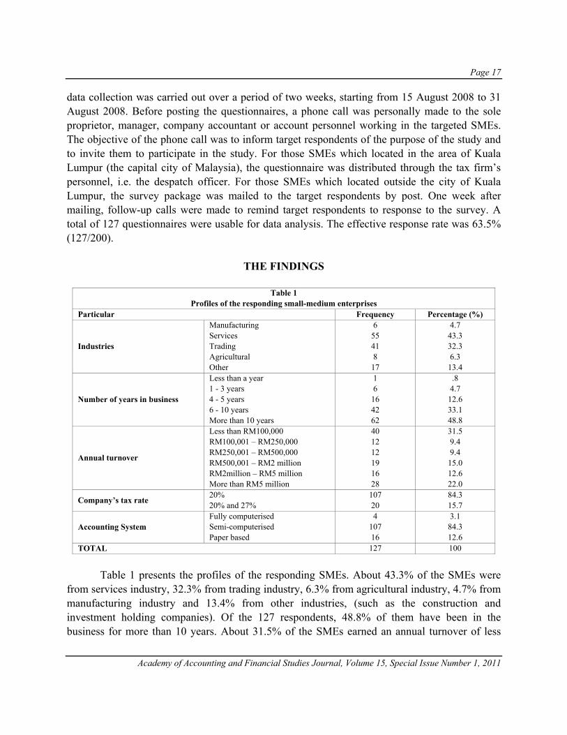
data collection was carried out over a period of two weeks, starting from 15 August 2008 to 31 August 2008. Before posting the questionnaires, a phone call was personally made to the sole proprietor, manager, company accountant or account personnel working in the targeted SMEs. The objective of the phone call was to inform target respondents of the purpose of the study and to invite them to participate in the study. For those SMEs which located in the area of Kuala Lumpur (the capital city of Malaysia), the questionnaire was distributed through the tax firm’s personnel, i.e. the despatch officer. For those SMEs which located outside the city of Kuala Lumpur, the survey package was mailed to the target respondents by post. One week after mailing, follow-up calls were made to remind target respondents to response to the survey. A total of 127 questionnaires were usable for data analysis. The effective response rate was 63.5% (127/200).
THE FINDINGS
Table 1 Profiles of the responding small-medium enterprises
Particular Frequency Percentage (%)
Industries
Manufacturing Services Trading Agricultural Other
6 55 41 8
17
4.7 43.3 32.3 6.3
13.4
Number of years in business
Less than a year 1 - 3 years 4 - 5 years 6 - 10 years More than 10 years
1 6
16 42 62
.8 4.7
12.6 33.1 48.8
Annual turnover
Less than RM100,000 RM100,001 – RM250,000 RM250,001 – RM500,000 RM500,001 – RM2 million RM2million – RM5 million More than RM5 million
40 12 12 19 16 28
31.5 9.4 9.4
15.0 12.6 22.0
Company’s tax rate 20% 20% and 27%
107 20
84.3 15.7
Accounting System Fully computerised Semi-computerised Paper based
4 107 16
3.1 84.3 12.6
TOTAL 127 100 Table 1 presents the profiles of the responding SMEs. About 43.3% of the SMEs were from services industry, 32.3% from trading industry, 6.3% from agricultural industry, 4.7% from manufacturing industry and 13.4% from other industries, (such as the construction and investment holding companies). Of the 127 respondents, 48.8% of them have been in the business for more than 10 years. About 31.5% of the SMEs earned an annual turnover of less
Page 18
Academy of Accounting and Financial Studies Journal, Volume 15, Special Issue Number 1, 2011
than RM100,000, 15% earned between RM500,001 to RM2 million and 12.6% earned between RM2 million to RM5 million [Note: at the time of writing, the exchange rate is 1 USD=RM3.3]. Majority (84.3%) of the SMEs indicated that in year of assessment (YA) 2007, the company tax rate was 20%, thus indicating that the chargeable income was RM500,000 or below. Notably, only a small portion of SMEs (15.7%) indicated that they were charged a tax rate of 20% and 27%, thus suggesting that their chargeable income was above RM500,000 in YA 2007. Only 3.1% of the SMEs had fully computerized the accounting system.
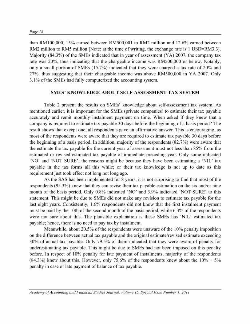
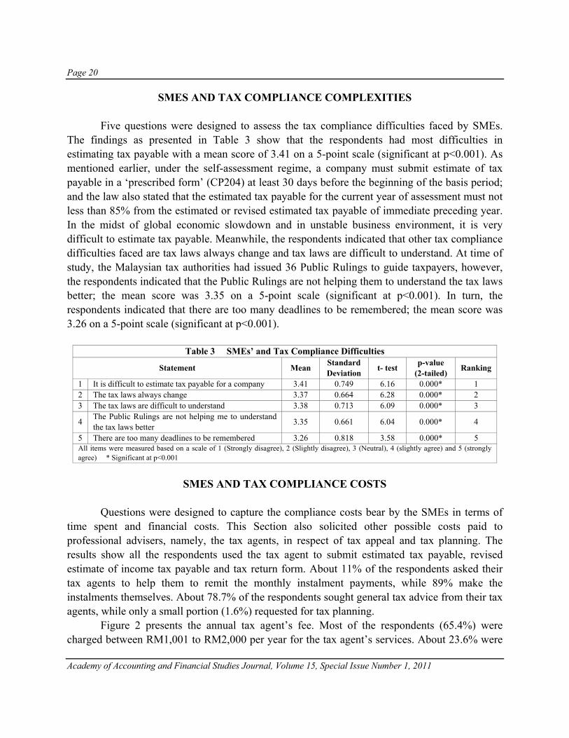
SMES’ KNOWLEDGE ABOUT SELF-ASSESSMENT TAX SYSTEM Table 2 present the results on SMEs’ knowledge about self-assessment tax system. As mentioned earlier, it is important for the SMEs (private companies) to estimate their tax payable accurately and remit monthly instalment payment on time. When asked if they knew that a company is required to estimate tax payable 30 days before the beginning of a basis period? The result shows that except one, all respondents gave an affirmative answer. This is encouraging, as most of the respondents were aware that they are required to estimate tax payable 30 days before the beginning of a basis period. In addition, majority of the respondents (82.7%) were aware that the estimate the tax payable for the current year of assessment must not less than 85% from the estimated or revised estimated tax payable of immediate preceding year. Only some indicated ‘NO’ and ‘NOT SURE’, the reasons might be because they have been estimating a ‘NIL’ tax payable in the tax forms all this while; or their tax knowledge is not up to date as this requirement just took effect not long not long ago. As the SAS has been implemented for 8 years, it is not surprising to find that most of the respondents (95.3%) knew that they can revise their tax payable estimation on the six and/or nine month of the basis period. Only 0.8% indicated ‘NO’ and 3.9% indicated ‘NOT SURE’ to this statement. This might be due to SMEs did not make any revision to estimate tax payable for the last eight years. Consistently, 1.6% respondents did not know that the first instalment payment must be paid by the 10th of the second month of the basis period, while 6.3% of the respondents were not sure about this. The plausible explanation is these SMEs has ‘NIL’ estimated tax payable; hence, there is no need to pay tax by instalment. Meanwhile, about 20.5% of the respondents were unaware of the 10% penalty imposition on the difference between actual tax payable and the original estimate/revised estimate exceeding 30% of actual tax payable. Only 79.5% of them indicated that they were aware of penalty for underestimating tax payable. This might be due to SMEs had not been imposed on this penalty before. In respect of 10% penalty for late payment of instalments, majority of the respondents (84.3%) knew about this. However, only 75.6% of the respondents knew about the 10% + 5% penalty in case of late payment of balance of tax payable.
Page 19
Academy of Accounting and Financial Studies Journal, Volume 15, Special Issue Number 1, 2011
Table 2 SMEs’ Knowledge about Self-assessment Tax System
Tax Knowledge Yes No Not sure
Frequency (percentage)
Frequency (percentage)
Frequency (percentage)
a. Do you know a company is required to estimate tax payable 30 days before the beginning of a basis period?
126 (99.2)
1 (0.8)
0 (0)
b. Do you know estimated tax payable must not less than 85% from the estimated or revised estimated tax payable of immediate preceding year?
105 (82.7)
9 (7.1)
13 (10.2)
c. Do you know a company can revise their tax payable estimation on the six and/or nine month?
121 (95.3)
1 (0.8)
5 (3.9)
d. Do you know a company need to make the first instalments by the 10th of the second month of the basis period?
117 (92.1)
2 (1.6)
8 (6.3)
e.
Do you know when actual tax payable exceeds the original estimate or the revised estimate by an amount exceeding 30% of the actual tax payable, the difference will be subject to a penalty of 10%?
101 (79.5)
7 (5.5)
19 (15.0)
f. Do you know there will be a 10% penalty for every late payment of instalments?
107 (84.3)
1 (0.8)
19 (15.0)
g. Do you know there will be a 10% + 5% penalty for a late payment of balance of tax payable?
96 (75.6)
8 (6.3)
23 (18.1)
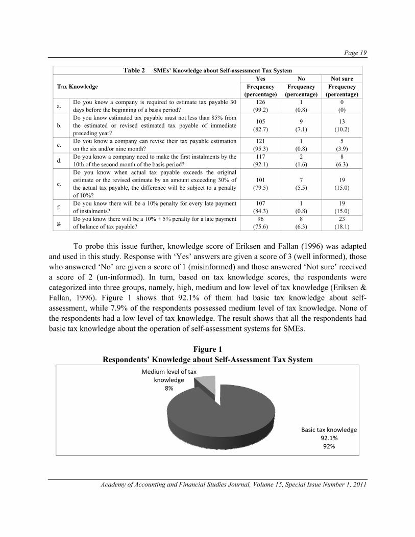
To probe this issue further, knowledge score of Eriksen and Fallan (1996) was adapted and used in this study. Response with ‘Yes’ answers are given a score of 3 (well informed), those who answered ‘No’ are given a score of 1 (misinformed) and those answered ‘Not sure’ received a score of 2 (un-informed). In turn, based on tax knowledge scores, the respondents were categorized into three groups, namely, high, medium and low level of tax knowledge (Eriksen & Fallan, 1996). Figure 1 shows that 92.1% of them had basic tax knowledge about self-assessment, while 7.9% of the respondents possessed medium level of tax knowledge. None of the respondents had a low level of tax knowledge. The result shows that all the respondents had basic tax knowledge about the operation of self-assessment systems for SMEs.
Figure 1 Respondents’ Knowledge about Self-Assessment Tax System
Basic tax knowledge92.1%92%
Medium level of tax knowledge
8%
Page 20
Academy of Accounting and Financial Studies Journal, Volume 15, Special Issue Number 1, 2011
SMES AND TAX COMPLIANCE COMPLEXITIES Five questions were designed to assess the tax compliance difficulties faced by SMEs. The findings as presented in Table 3 show that the respondents had most difficulties in estimating tax payable with a mean score of 3.41 on a 5-point scale (significant at p<0.001). As mentioned earlier, under the self-assessment regime, a company must submit estimate of tax payable in a ‘prescribed form’ (CP204) at least 30 days before the beginning of the basis period; and the law also stated that the estimated tax payable for the current year of assessment must not less than 85% from the estimated or revised estimated tax payable of immediate preceding year. In the midst of global economic slowdown and in unstable business environment, it is very difficult to estimate tax payable. Meanwhile, the respondents indicated that other tax compliance difficulties faced are tax laws always change and tax laws are difficult to understand. At time of study, the Malaysian tax authorities had issued 36 Public Rulings to guide taxpayers, however, the respondents indicated that the Public Rulings are not helping them to understand the tax laws better; the mean score was 3.35 on a 5-point scale (significant at p<0.001). In turn, the respondents indicated that there are too many deadlines to be remembered; the mean score was 3.26 on a 5-point scale (significant at p<0.001).
Table 3 SMEs’ and Tax Compliance Difficulties
Statement Mean Standard Deviation t- test p-value
(2-tailed) Ranking
1 It is difficult to estimate tax payable for a company 3.41 0.749 6.16 0.000* 1 2 The tax laws always change 3.37 0.664 6.28 0.000* 2 3 The tax laws are difficult to understand 3.38 0.713 6.09 0.000* 3
4 The Public Rulings are not helping me to understand the tax laws better 3.35 0.661 6.04 0.000* 4
5 There are too many deadlines to be remembered 3.26 0.818 3.58 0.000* 5 All items were measured based on a scale of 1 (Strongly disagree), 2 (Slightly disagree), 3 (Neutral), 4 (slightly agree) and 5 (strongly agree) * Significant at p<0.001
SMES AND TAX COMPLIANCE COSTS
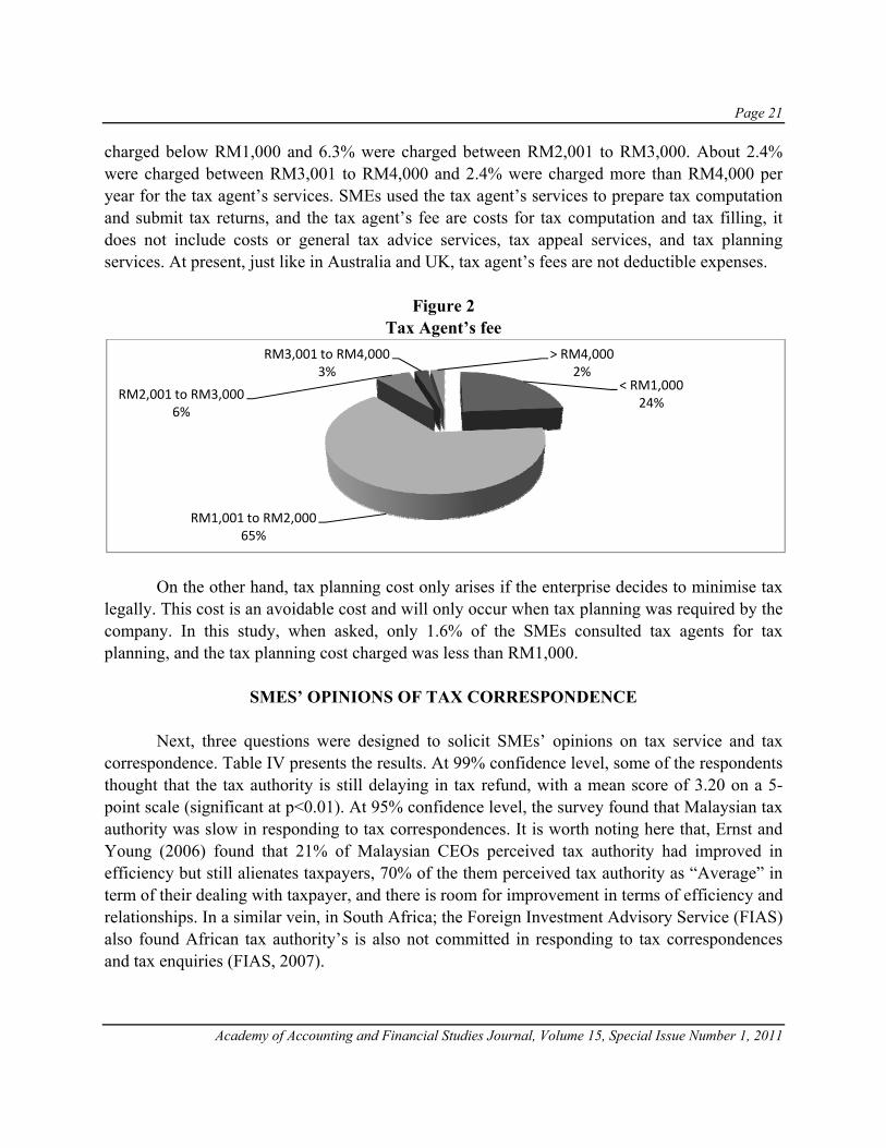
Questions were designed to capture the compliance costs bear by the SMEs in terms of time spent and financial costs. This Section also solicited other possible costs paid to professional advisers, namely, the tax agents, in respect of tax appeal and tax planning. The results show all the respondents used the tax agent to submit estimated tax payable, revised estimate of income tax payable and tax return form. About 11% of the respondents asked their tax agents to help them to remit the monthly instalment payments, while 89% make the instalments themselves. About 78.7% of the respondents sought general tax advice from their tax agents, while only a small portion (1.6%) requested for tax planning. Figure 2 presents the annual tax agent’s fee. Most of the respondents (65.4%) were charged between RM1,001 to RM2,000 per year for the tax agent’s services. About 23.6% were
Page 21
Academy of Accounting and Financial Studies Journal, Volume 15, Special Issue Number 1, 2011
charged below RM1,000 and 6.3% were charged between RM2,001 to RM3,000. About 2.4% were charged between RM3,001 to RM4,000 and 2.4% were charged more than RM4,000 per year for the tax agent’s services. SMEs used the tax agent’s services to prepare tax computation and submit tax returns, and the tax agent’s fee are costs for tax computation and tax filling, it does not include costs or general tax advice services, tax appeal services, and tax planning services. At present, just like in Australia and UK, tax agent’s fees are not deductible expenses.
Figure 2 Tax Agent’s fee
On the other hand, tax planning cost only arises if the enterprise decides to minimise tax legally. This cost is an avoidable cost and will only occur when tax planning was required by the company. In this study, when asked, only 1.6% of the SMEs consulted tax agents for tax planning, and the tax planning cost charged was less than RM1,000.
SMES’ OPINIONS OF TAX CORRESPONDENCE Next, three questions were designed to solicit SMEs’ opinions on tax service and tax correspondence. Table IV presents the results. At 99% confidence level, some of the respondents thought that the tax authority is still delaying in tax refund, with a mean score of 3.20 on a 5-point scale (significant at p<0.01). At 95% confidence level, the survey found that Malaysian tax authority was slow in responding to tax correspondences. It is worth noting here that, Ernst and Young (2006) found that 21% of Malaysian CEOs perceived tax authority had improved in efficiency but still alienates taxpayers, 70% of the them perceived tax authority as “Average” in term of their dealing with taxpayer, and there is room for improvement in terms of efficiency and relationships. In a similar vein, in South Africa; the Foreign Investment Advisory Service (FIAS) also found African tax authority’s is also not committed in responding to tax correspondences and tax enquiries (FIAS, 2007).
< RM1,00024%
RM1,001 to RM2,00065%
RM2,001 to RM3,0006%
RM3,001 to RM4,0003%
> RM4,0002%

Page 22
Academy of Accounting and Financial Studies Journal, Volume 15, Special Issue Number 1, 2011
Table IV SMEs’ Opinion on Tax Correspondence with the Inland Revenue Board Malaysia
Statement Mean Standard Deviation t-test p-value
(2-tailed) Ranking
1 IRBM always delay tax refund to my company 3.20 0.705 3.271 0.001** 1
2 IRBM is slow in responding to tax correspondence 3.11 0.523 2.376 0.019* 2
3 IRBM’s advice is not sufficiently accessible 3.05 0.434 1.227 0.222 3
All items were measured based on a scale of 1 (Strongly disagree), 2 (Slightly disagree), 3 (Neutral), 4 (slightly agree) and 5 (strongly agree). * Significant at p<0.05; ** Significant at p<0.01
IMPLICATIONS OF THE STUDY
This study found Malaysian SMEs are struggling to understand and comply with the tax laws, and most SMEs found that the Public Rulings are not helping them to understand the tax laws better. The findings suggest that to understand SMEs tax compliance problem, greater efforts must be done by tax authorities to enable SMEs to communicate with them face to face, via phone or electronic mails. Notably, although the Malaysian tax authority had embraced an electronic tax filing system, however, with regard to tax correspondence, the IRBM is still maintaining the traditional methods of communication with taxpayers via postal mail and phone calls instead of using electronic mails. It is argued that the speed of tax correspondence can be improved via electronic mails. This study support the call of Alam (2009) that the government ministries and agencies that are responsible for promoting SMEs adoption of internet technologies to focus in establishing a closer relationship between SMEs and other business parties by harnessing the powers of cutting edge technologies. In addition, extant study of Chibelushi and Costello (2009) suggested that government policy makers aiming to support SMEs to use ICT to achieve greater competitive advantage need to consider various problem faced by SMEs in technology adoption. The results also indicate that most SMEs merely engaged tax agents for annual tax compliance matters rather than for tax planning purposes. This finding is in contrast with Ernst and Young (2006) survey’ which found that big companies (in particular the public listed company) placed the greatest value of the tax function in the ability to tax-plan and minimise the effective tax rate. Nonetheless, this study affirms the assertion of Poopathi (2009) that SMEs are motivated by cost when purchasing tax service from accountants. In practice, it is costly to engage tax agent to device tax planning strategies to meet the specific needs, such as the application of tax incentive and tax dispute resolution for SMEs. The findings also suggest that the IRBM to simplify the self-assessment system for SMEs, and to make it more taxpayer-friendly and practical. For example, in view of economic downturn, the estimation of tax payable should not be restricted to at least 85% from the
Page 23
Academy of Accounting and Financial Studies Journal, Volume 15, Special Issue Number 1, 2011
estimated or revised estimated tax payable of the immediate preceding year. In addition, a single revision in the ninth month of the basis period will also reduce the numbers of deadlines to be remembered. The IRBM should simplify record keeping requirement for small businesses. It is suggested that SMEs (private limited companies) with paid up share capital of less than RM2.5 million need not send their accounts for external audit, hence this would save cost and hassle. Such move would also enable SMEs to have more resources in doing and growing their business.
CONCLUSION The issue of SMEs and taxation has attracted much attention, however, globally; systematic study on tax compliance complexities faced by SMEs in the post self-assessment system is scant. This study presents tax compliance complexities faced by SMEs in a developing country like Malaysia. Nonetheless, this study has some limitations. Firstly, the sample was confined to SMEs who were corporate clients of a tax firm. The findings may not be generalised to a larger population. Secondly, due to little study on SMEs and tax compliance in the post self-assessment system in Malaysia and worldwide, there is limited reference point that can be relied on for comparison. Last but not least, this is a cross-sectional survey, whereby data was collected at a particular point of time; as such the respondents’ opinion may change over time. A nationwide study can be conducted in the future to gain a clearer picture. Longitudinal studies over a period of five years, for an instance, will provide a useful and interesting picture on how SMEs and tax compliance issue evolve over a period of time. In addition, comparative studies can also be done on SMEs in different countries across the regions.
REFERENCES Abdul-Jabbar, H., & Pope, J. (2008). The effects of self-assessment system on the tax compliance costs of small and
medium enterprises in Malaysia. Australian Tax Forum, 23, 289-306. Abrie, W., & Doussy, E. (2006). Tax compliance obstacles encountered by small and medium enterprises in South
Africa. Meditari Accountancy Research, 14(1), 1-13. Alam, S. S. (2009). Adoption of internet in Malaysian SMEs. Journal of Small Business and Enterprise
Development, 16(2), 240-255. Arachi, G., & Santoro, A. (2007). Tax enforcement for SMEs: lessons from the Italian experience. eJournal of Tax
Research, 5(2), 225-243. Bulbir, S. (2003, 25 September 2003 ). IRB should settle payments promptly. The Star, Central Bank of Malaysia. (2005). Definitions for Small and Medium Enterprises in Malaysia. Retrieved 22 May
2009. from http://www.smeinfo.com.my/pd/sme_definition_ENGLISH.pdf.

Page 24
Academy of Accounting and Financial Studies Journal, Volume 15, Special Issue Number 1, 2011
Central Bank of Malaysia. (2007). Small Medium Enterprise Annual Report 2006 [Electronic Version]. Retrieved 21 May 2009, from www.bnm.gov.my
Chibelushi, C., & Costello, P. (2009). Challenges facing W. Midlands ICT-Oriented SMEs. Journal of Small
Business and Enterprise Development, 16(2), 210-229. Concern Taxpayer. (1997, 25 October 1997). Seeking help from IRD. The Star, Eriksen, K., & Fallan, L. (1996). Tax knowledge and attitudes towards taxation: A report on quasi-experiment.
Journal of Economic Psychology, 17, 387-402. Ernst and Young (Ed.). (2006). Annual Tax Survey. Malaysia. Evans, C., Carlon, S., & Massey, D. (2005). Record Keeping Practices and Tax Compliance of SMEs. eJournal of
Tax Research, 3(2), 288-334. FIAS. (2007). South Africa Tax Compliance Burden For Small Businesses: A Survey of Tax Practitioners
[Electronic Version]. Retrieved 12 July 2008, from www.fias.net and Report – Final 29+Aug.pdf Hanefah, M., Ariff, M., & Kasipillai, J. (2001). Compliance cost of small and medium enterprises. Journal of
Australian Taxation, 4(1), 73-97. Lee, T. L. (1997, 30 August 1997). Long wait for tax refunds. The Star Mckerchar, M. (2005). The impact of income tax complexity on practitioners in Australia. Australian Tax Forum: a
Journal of Taxation Policy, Law and Reform, 20(4), 529-554. Poopathi, P. M. (2009). What SMEs want. Accountants Today, 22(4), 8-10. Puran. (1997, 30 August 1997). At one’s wits end trying to solve tax woes. The Star, Vos AM, D. R., & Mihail, T. (2006). The importance of certainty and fairness in a self-assessing environment.
Retrieved. from http://www.igt.gov.au/content/media/ATAX_paper April_2006.pdf.
Page 25
Academy of Accounting and Financial Studies Journal, Volume 15, Special Issue Number 1, 2011
MODELING COST BEHAVIOR: LINEAR MODELS FOR COST STICKINESS
Arnel Onesimo O. Uy, De La Salle University
ABSTRACT
Literature acknowledges that costs might not be linear and proportional with activity levels. However, conjectures about the sticky behavior of costs are largely based on anecdotal and empirical evidence despite sufficiently advanced economic theory that explains cost behavior (Cooper and Kaplan, 1998; Noreen and Soderstrom, 1997; Banker and Johnston, 1993). For instance, while Noreen and Soderstrom (1997) find no evidence of stickiness, Anderson, et al (2003) find that SG&A costs are sticky – that is, they increase, on the average, by 0.55% per 1% increase in revenues, but decline by 0.35% per 1% decrease in revenues. Subramaniam and Weidenmier (2003) confirm cost stickiness, finding that total cost increase 0.93% per 1% increase in revenues but decrease only by 0.85% per 1% decrease in revenues. Both studies used data from US firms. This paper derived a basic cost behavior model and used this model to test whether asymmetric cost behavior in Philippine firms is also prevalent, using different linear models such as OLS and GLS regression analyses. It concluded that GLS regression analysis is not more efficient than OLS regression analysis.
INTRODUCTION The relationship between cost and activity has always baffled business executives. While it was commonly accepted that there exist a relationship between the two, literature has not clearly explained the relationship. Some costs are acknowledged to move linearly and proportionally with activity levels while others don’t. In more recent studies, the issue of symmetric movement of costs with respect to activity level changes was also discussed. Anderson, Banker and Janakiraman (2003) coined the term “sticky” costs to describe what they discovered as asymmetric cost behavior with respect to activity levels. To shed light on this topic, I will first derive a basic cost behavior model which will allow us to test asymmetric cost behavior in firms. Next I will use Philippine company data from 2004 to 2008 and run different linear models, particularly OLS and GLS regression analyses and discuss the results for each. By way of conclusion, I will present which liner cost model is more efficient

Page 26
Academy of Accounting and Financial Studies Journal, Volume 15, Special Issue Number 1, 2011
PART 1: BASIC COST BEHAVIOR MODEL 1.1 Deriving the cost behavior Model To model cost behavior using economic theory, we start by deriving the cost-volume-relationships from the cost and production function. This will provide economic grounding which underlies the sticky cost hypothesis and the economic models used to test it. The cost function relates total cost (c) to factor prices (pj) and output quantity (y). In competitive markets, factor prices and output quantity are exogenous. A widely used production function in economics is the Cobb-Douglas production function:
βαttttt xxAxxfy 21211 ),( ⋅== (1)
where t is a time index, At is a positive constant, xjt , j=1,2 are input factors and α, β are positive, time-invariant fractions that add up to one which implies constant returns to scale. The corresponding Cobb-Douglas cost function is:
)/(1)( βα+= tttt yKyc (2)
where Kt is a function of factor princes (pj), At, α and β.The cost growth between t-1 and t can be expressed as
)/(1
1111 )()(
βα+
−−−−⎟⎟⎠
⎞⎜⎜⎝
⎛=
t
t
t
t
tt
tt
yy
KK
ycyc
(3) If we take the log of both sides and (implicitly) assume that factor prices are constant over time, we are able to derive an empirical model shown as equation (4) below. If we do not assume constant factor prices, our model will suffer from omitted variable bias, unless we consider factor prices in our empirical estimation.
tt
t
t
t
yy
cc
εγγ +⎟⎟⎠
⎞⎜⎜⎝
⎛+=⎟⎟
⎠
⎞⎜⎜⎝
⎛
−− 110
1
log)
log (4)
with ⎟⎟⎠
⎞⎜⎜⎝
⎛=
−10 log
t
t
KK
γ , βα
γ+
=1
1 , and tε being a zero mean error term.

Page 27
Academy of Accounting and Financial Studies Journal, Volume 15, Special Issue Number 1, 2011
This model is consistent with our traditional fixed- and variable-cost model. Traditional model assumes that variable costs change proportionately with the changes in activity level
which implies a constant returns to scale, 11 =γ since 1=+ βα . Moreover, the model assumes that the change in variable costs is invariant to the direction of the change in volume. Thus, the
cost-volume-relationship is symmetric for volume increases and decreases, implying that 1γ is equal in both cases. However, this runs counter to the recent empirical studies (Anderson, et al, 2003; Calleja, 2005; Anderson and Lanen, 2007) which provide evidence that certain cost types, particularly SG&A costs, behave in an asymmetric manner. They rise more with increases in volume than
they fall with decreases in volume thereby implying that 1γ should be higher for increases that for decreases in activity level. Extant literature defines this asymmetric cost behavior with respect to directions in volume changes as sticky cost or cost stickiness, and typically uses SG&A costs instead of total cost and sales instead of volume to test this behavior. It is interesting to point out that while Anderson et al. (2003) whose study introduced us to the concept of cost stickiness, explain their measurement choice with a lack of large datasets on activity levels and total costs, Anderson and Lanen (2007) warn that changes in sales is not an exogenous regressor because in addition to volume, sales depend on prices, which are set by management. Anderson and Lanen (2007) also point out that the classification of costs is subject to managerial choice and that SG&A represents only about 30% of total cost. Consequently, these create measurement problems for investigating cost behavior. In any case, to test the sticky cost hypothesis, we extend equation (4) to allow different slopes for positive and negative volume changes, shown as equation (5) below.
tt
tt
t
t
t
t
yyD
yy
cc εγγγ +⎟⎟
⎠
⎞⎜⎜⎝
⎛+⎟⎟
⎠
⎞⎜⎜⎝
⎛+=⎟⎟
⎠
⎞⎜⎜⎝
⎛
−−− 12
110
1
logloglog (5)
where 1=tD if ,0<Δ ty and 0=tD if 0>Δ ty . We then use Anderson et al’s 2003 measurement choices and substitutes to yield equation (6) below:
tt
tt
t
t
t
t
SALESSALESD
SALESSALES
ASGASG εγγγ +⎟⎟
⎠
⎞⎜⎜⎝
⎛+⎟⎟
⎠
⎞⎜⎜⎝
⎛+=⎟⎟
⎠
⎞⎜⎜⎝
⎛
−−− 12
110
1
loglog&&log (6)
where 1=tD if ,0<Δ tSALES and 0=tD if 0>Δ tSALES .
The coefficient, 1γ , measures the percentage increase in SG&A costs with a 1% increase
in sales, while the combined coefficients, )( 21 γγ + measures the percentage decrease in SG&A costs with a 1% decrease in sales. In the traditional fixed- and variable-cost model, it proposes
Page 28
Academy of Accounting and Financial Studies Journal, Volume 15, Special Issue Number 1, 2011
that total cost changes are invariant to the direction of the change in activity, which means that 02 =γ . This was refuted by Anderson et al. (2003) when they found that on the average, cost
increase by 0.55% per 1% increase in sales, but decline by 0.35% per 1% decrease in sales, thus 02 <γ .
1.2 Explaining cost stickiness Literature has identified three major factors that contribute to the asymmetry in SG&A costs with respect to increases and decreases in sales revenue. First is the fixity of SG&A costs. When a portion of SG&A costs is fixed and sales decline, the ratio between SG&A costs and sales increases, because the fixed capacity costs are spread over a lower sales level. This includes also costs which are contractual in nature which cannot be discontinued with decreases in sales volume. The next two factors are related to the part of SG&A costs that are variable. Second, when the level of activity declines, the manager decides whether to adjust capacity in order to reduce variable SG&A costs. If the manager maximizes the value of the firm, he will trade off the costs of maintaining excess resources against the adjustment costs of cutting existent resources and building them up again, when demand is restored. His decision depends on his expectation of future demand and on the uncertainty of his expectation. If the manager expects demand to restore sufficiently fast in future periods, adjustment costs will be higher than the costs of unutilized capacity and he will decide to maintain excess resources. Similarly, if the uncertainty about future demand is high and cutting committed resources costly, the manager will decide to wait in order to obtain more information before incurring adjustment costs. The asymmetry in costs induced by the economic decision to bear the costs of excess resources is defined as cost stickiness. Third, an asymmetric cost behavior with respect to sales increases and decreases will also arise, if the manager maintains excess capacity maximizing his own utility function, whereas the firm value maximizing decision would be to cut recourses. In this case, the manager expects a permanent decline in future demand yet, he decides to keep capacity because he incurs a higher disutility with understaffing than with overstaffing. For example, in the case of managerial empire building, managers might be willing to maintain unutilized resources for reasons such as status, prestige and power (Jensen and Meckling, 1976; Hope and Thomas, 2007) Another reason why managers might be reluctant to cut resources, particularly staff, is when they face considerable public pressure with regard to their social responsibility. Stickiness might also be affected by the systems of corporate governance and managerial oversight. In the US and UK, for instance, the common law system of corporate governance puts more emphasis on the notion of shareholder maximization and on the role of the stock market as a means of achieving that objective. The stock market is also the mechanism through which the
Page 29
Academy of Accounting and Financial Studies Journal, Volume 15, Special Issue Number 1, 2011
market for corporate control operates to discipline underperforming management. Thus, management comes under external pressure to make decisions in the interest of shareholders. In contrast, the systems of corporate governance in France and Germany, rather than being exclusively directed at shareholder levels, are directed at a coalition of external and internal interest groups. This then carries over to an increased role of co-determination between management, workers, and fund providers in the allocation of resources. O’Sullivan (2003) describes this regulatory framework in France as one “which provides more social protection to their workers than is the case in the US. There are, for instance, substantial costs to French enterprises downsizing their labor forces”. He likewise recognized a broadly similar governance framework of co-determination existing in Germany where firm employees sit either on the Supervisory Board (the Aufsichtsrat) or the factory council (the Betriebsrat). Both of these councils have “the capacity to negotiate wages, job security and other aspects of the age relationship that is largely absent in countries such as US and UK”. Because of these features (the higher relative cost of cutting back resources, the level of external oversight of managerial behavior, and the focus on stakeholders rather than shareholders) may largely affect cost stickiness in not only in French and German firms in particular but in firms with these governance systems in general.
PART 2: TESTING COST STICKINESS 2.1 Data Description The primary variables used in my analysis are SG&A costs and sales revenues. The dataset I used includes annual data for listed Philippine firms belonging to 17 industries covering 5 years from 2004 and 2008. I screened the data for missing observations in SG&A or sales revenue in the current and preceding year and deleted observation if SG&A costs exceeded sales revenues. The total number of remaining observations is 634 for 173 firms, an average of 3.62 observations per firm. Table 1 provides descriptive information about the annual revenues and SG&A costs for the observations included in the dataset. The mean value of SG&A costs as a percentage of sales is 87.68% with median of 91.48% and standard deviation of 90.91%. Panel B provides information about the frequency of firm-years when revenue fell (relative to the previous year) and firm-years when SG&A fell. Revenue fell in 30.18% of the annual firm-years in the sample and SG&A fell 29.86%. The mean value of revenue decrease is 23.21% with median of 16.21% and standard deviation of 23.98%, and the mean value of decreases in SG&A is 23.48% with a median of 19.56% and standard deviation of 22.54%.

Page 30
Academy of Accounting and Financial Studies Journal, Volume 15, Special Issue Number 1, 2011
Table 1Summary StatisticsAll reported numbers are in P'000 except the percentages
Panel A: Distribution of Annual Revenue and SG&A Costs from 2004 to 2008
Mean MedianStandard Deviation
Sales Revenues 10,429,453 1,178,591 29,449,055 Selling, general and 9,144,041 1,078,127 26,773,433 administrative (SG&A) costsSG&A costs as a percentage 87.68% 91.48% 90.91% of revenues
Panel B: Periodic Fluctuations in Revenues and SG&A from 2004 to 2008
% of firm-years with negative %
change
Mean % decrease
across periods
Median % decreases
across periods
Standard Deviation of %
decreases across periods
Sales revenues 30.18% 23.31% 16.21% 23.98%SG&A costs 29.86% 23.48% 19.56% 22.54%
2.2 OLS Estimation
Table 2 Summary Statistics (Stata 9.1)
Using the model in equation (6) applied on a cross-sectional analysis of a wide variety of industries and large differences in the size of firms. Because of this, the ratio form and the log specification improve the comparability of the variables across firms and alleviates potential
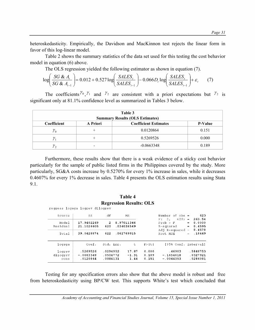
Page 31
Academy of Accounting and Financial Studies Journal, Volume 15, Special Issue Number 1, 2011
heteroskedasticity. Empirically, the Davidson and MacKinnon test rejects the linear form in favor of this log-linear model. Table 2 shows the summary statistics of the data set used for this testing the cost behavior model in equation (6) above. The OLS regression yielded the following estimator as shown in equation (7).
tt
tt
t
t
t
t
SALESSALESD
SALESSALES
ASGASG ε+⎟⎟
⎠
⎞⎜⎜⎝
⎛−⎟⎟
⎠
⎞⎜⎜⎝
⎛+=⎟⎟
⎠
⎞⎜⎜⎝
⎛
−−− 111
log066.0log527.0012.0&&log (7)
The coefficients 0γ , 1γ and 2γ are consistent with a priori expectations but 2γ is significant only at 81.1% confidence level as summarized in Tables 3 below.
Table 3 Summary Results (OLS Estimates)
Coefficient A Priori Coefficient Estimates P-Value
0γ + 0.0120864 0.151
1γ + 0.5269526 0.000
2γ - -0.0663348 0.189
Furthermore, these results show that there is a weak evidence of a sticky cost behavior particularly for the sample of public listed firms in the Philippines covered by the study. More particularly, SG&A costs increase by 0.5270% for every 1% increase in sales, while it decreases 0.4607% for every 1% decrease in sales. Table 4 presents the OLS estimation results using Stata 9.1.
Table 4 Regression Results: OLS
Testing for any specification errors also show that the above model is robust and free from heteroskedasticity using BP/CW test. This supports White’s test which concluded that

Page 32
Academy of Accounting and Financial Studies Journal, Volume 15, Special Issue Number 1, 2011
heteroskedasticity was not a problem for the loglinear model. To determine whether the model has committed the violation of multicollinearity or the presence of a linear relationship among the variables, I performed the Variance Inflation Factor (VIF) Criterion Test, which states that if any VIFj, where j = 2,3,…k, and k = the number of treatments (independent variables), has a VIF value greater than 10, there is an evidence of multicollinearity and correcting actions should be directed towards removing the erring variable or retaining it if an error of omission will take place. The computed VIF for the model passed this criteria. Lastly there was also no omitted variables in the model as shown by the Ramsey test. The results of these test are shown in Table 5.
Table 5 Specification Tests
Test for Heteroskedasticity
Test for Multicollinearity
Test for Omitted Variables
2.3 GLS Estimation In this section, I present the results of the GLS estimation. The GLS or generalized least squares estimator makes stronger distributional assumptions about the variance of the error term in our model (equation 6). However, it is nonetheless possible to obtain standard errors of GLS estimator that are robust to misspecifications of error variance just as in the OLS case. Interestingly, we can note that the resulting estimation of the model is similar to the OLS
model. Specifically, we see that the coefficients 0γ , 1γ and 2γ are consistent with a priori

Page 33
Academy of Accounting and Financial Studies Journal, Volume 15, Special Issue Number 1, 2011
expectations. They are significant except for 2γ which is significant only at 81.1% confidence level. This signifies that the OLS is still the best linear unbiased estimator for our cost behavior model. Stata results are shown in Table 6..
Table 6 Regression Results: GLS Estimates
CONCLUSION In this study, I found weak support that SG&A costs exhibit sticky behavior for listed Philippine firms. On the average across all firm-years in my observations, SG&A costs increased around 0.5270% for every 1% increase in sales but decline only 0.4607% per 1% decrease in sales. This is consistent with the alternative cost behavior model that takes into account the asymmetric friction created by managers when adjusting committed resource following changes in the level of activity of the firm albeit to a limited sense. From a modeling standpoint, we see that since there is no need for robust standard errors to be used for efficiency gains, then the GLS estimator is not more efficient than the OLS estimator (i.e. both show the same results). By showing these, we were able to simulate the Gauss-Markov theorem using Philippine data.

Page 34
Academy of Accounting and Financial Studies Journal, Volume 15, Special Issue Number 1, 2011
REFERENCES Anderson, M., Banker, R., Janakiraman, S. (2003). Are selling, general, and distribution costs sticky? J. Account.
Res. 41 (1), 47–63. Anderson, S., W. Lanen (2007). Understanding cost management: What can we learn from the evidence on “Sticky
Costs”?. Working Paper, University of Michigan. Banker, R., H. Johnston. (1993). "An Empirical Study of Cost Drivers in the U.S. Airline Industry." Accounting
Review 68 (July): 576-601. Calleja, K.; M. Steliaros; D. Thomas. (2006). A note on cost stickiness: Some International Comparisons.
Management Accounting Research 17, 127-140. Cooper, R., Kaplan, R. (1998). The Design of Cost Management Systems—Text and Cases, 2nd ed. Prentice Hall
Inc., New Jersey. Hope, O., and W. B. Thomas. (2007). Managerial empire building and firm disclosures. Journal of Accounting
Research, forthcoming. Jensen M. C, W. H. Meckling. (1976). "Theory ofthe Firm: Managerial Behavior, Agency Costs and Ownership
Structure." F=mal of Financial Economics S (October): 305-60. Noreen, E.; N. Soderstrom. (1994). "Are Overhead Costs Strictly Proportional to Activity? Evidence from Hospital
Service Departments." Joumal of Accounting and Economics 17 (January): 255-78. ---. (1997). 'The Accuracy of Proportional Cost Models: Evidence from Hospital Service Departments." Review of
Accounting Studies 2 (1997): 89-114. O’Sullivan, M., (2003). The political economy of comparative corporate governance. Rev. Int. Polit. Econ. 10 (1),
23–72. Subramaniam, C.,Weidenmier, M. (2003). Additional evidence on the sticky behaviour of costs. Working Paper,
Texas Christian University.
Page 35
Academy of Accounting and Financial Studies Journal, Volume 15, Special Issue Number 1, 2011
THE SECURITIES LITIGATION REFORM AND MARKET REACTIONS TO ANALYST
RECOMMENDATION REVISION
Huabing (Barbara) Wang, West Texas A&M University
ABSTRACT We examine the effect of the Securities Litigation Reform (SLR), namely, the Private Securities Litigation Reform of 1995 (PSLRA) and the Securities Litigation Uniform Standards Act of 1998 (SLUSA), on analyst research impact. We document a significant price-impact increasing effect of SLR on analyst recommendation revisions after controlling for recommendation-level characteristics and analyst experiences. We also find that firms more likely affected by SLR experience larger increases following PSLRA (both upgrades and downgrades) and SLUSA (downgrades only), suggesting that the price-impact increase is attributable to SLR rather than contemporaneous factors.
INTRODUCTION Complementing prior literature on regulatory changes (e.g., Gintschel & Markov, 2004), we examine the impact of the Securities Litigation Reform (SLR) on analyst research impact. SLR, namely, the Private Securities Litigation Reform of 1995 (PSLRA) and the Securities Litigation Uniform Standards Act of 1998 (SLUSA), gives public companies a safe harbor for forward-looking information. We define the impact of analyst recommendation revisions as the three-day abnormal returns starting on the revision date. Using a fixed effect model with analyst-firm effect fixed, we find that SLR has a significant price-impact increasing effect on analyst recommendation revisions, after controlling for recommendation-level characteristics and analyst experiences. Our results might be driven by contemporaneous factors. To exclude compounding influences, as in Johnson, Kasznik & Nelson (2001), we examine how SLR effect varies for firms with different ex ante litigation risk. We show that firms with higher ex ante litigation risk experience larger increases following PSLRA (both upgrades and downgrades) and SLUSA (downgrades only), largely in consistent with the analyst impact increasing effect of SLR. The remainder of the paper is organized as follows. In Section 2, we discuss the background of the SLR, review related literature, and develop hypotheses. Section 3 describes our sample selection process and research methodology. The main results, their interpretations, and robustness checks are contained in Section 4. Section 5 concludes.
Page 36
Academy of Accounting and Financial Studies Journal, Volume 15, Special Issue Number 1, 2011
SLR AND THE IMPACT OF ANALYST RESEARCH In the late 1980s, strike suits, the often meritless class action lawsuits filed in response to a drop in a stock's price and alleging that some disclosure (or failure to make disclosure) was either false or misleading, began to mushroom. According to an article in Forbes1, in the decade prior to 1995 more than half of the 150 top high-tech companies in Silicon Valley had been sued for securities fraud. Ninety-three percent settled, paying an average settlement of $8.6 million. Consequently, it is understandable that many public companies, especially those high-technology firms, chose to refrain from disclosing beyond the minimum required by securities laws. According to a National Investor Relations Institute survey conducted in the summer of 1995, only 20 percent of companies responded to the survey indicated that they "routinely" or "occasionally" forecast quarterly or annual results.2 Thus, investors did not always have access to the important information known to the management that could affect their investment decisions. Besides, since trial lawyers usually obtained the lion’s share out of the final settlement, it was argued that these lawsuits only benefited lawyers yet harmed the interest of shareholders as a whole. In response to this, Congress proposed PSLRA, aimed at amending the federal securities laws to curb certain abusive practices in private securities litigation. The legislation was passed by both Houses of Congress in mid 1995 and eventually reached President Clinton in mid-December. President Clinton vetoed the legislation, yet both the House and Senate overrode the veto, and the legislation became law on December 22, 1995. The new law made it tougher to bring federal securities claims against public companies. The most important yet controversial aspect of the new law is the safe harbor provision. Section 102 of the law states that it provides certain issuers of securities a safe harbor from liability for forward-looking statements regarding a security’s projected performances or operations, if: (1) the statement is immaterial or is identified as a forward-looking statement and accompanied by certain cautionary statements; or (2) the plaintiff fails to prove that the statement was made with either actual knowledge of its false or misleading nature by a natural person, or actual approval by an executive officer. The safe harbor provision applies to both written and oral statements. Overall, the safe harbor provision enables executives of public companies to share with the market their projections of the companies’ future without the fear of being sued if their projections fail to materialize. PSLRA was designed to encourage more complete disclosure by public companies, but it had a loophole: plaintiffs’ lawyers could circumvent it by filing their cases in the state courts. As documented by Grundfest & Perino (1997), the overall litigation rate following PSLRA has actually increased. As a result, public companies may remain reluctant to disclose even with the safe harbor provision in PSLRA. To close the loophole, both Houses of Congress passed the legislation of SLUSA to set uniform national standards for class-action shareholder suits involving nationally-traded securities (securities listed on the New York Stock Exchange, NASDAQ or the American Stock Exchange) in July 1998. The legislation became public law on
Page 37
Academy of Accounting and Financial Studies Journal, Volume 15, Special Issue Number 1, 2011
November 3, 1998. The new law significantly limits the ability of plaintiff-investors to seek redress for securities fraud under state law and through state courts. Bringing the most sweeping revisions of the federal securities laws since the 1930s (Lerach, 1998), SLR has a profound effect on the information environment. On the one hand, proponents of SLR point to the benefit of increased voluntary disclosure and argue that SLR can help create a more desirable information environment and benefit investors and the economy in general. Many practitioner accounts indicate that firms indeed have become more open and forward-looking and that the communication between companies and the analyst community has improved following SLR. For example, Bruce Nakao, senior vice president at Adobe Systems Inc, said that the new law (PSLRA) made it more comfortable to give indications of where a company was going, and he expected to see more forward-looking information in verbal communications with analysts in conference calls or analyst meetings.3 On the other hand, SLR faces harsh criticism as to its effect on the quality of corporate disclosure. First, the concern has been raised that SLR might give corporations “a license to lie”, as stated by Senator Joseph R. Biden.4 Even if firms do not knowingly give out misleading information, SLR does give public companies more latitude to discuss the companies’ prospect with optimism, and this optimism may mislead analysts and investors. Consequently, the information disclosed may be so uncertain that the information environment actually deteriorates following SLR. A number of authors have examined the impact of the safe harbor provision of PSLRA on the information environment. Spiess & Tkac (1997) and Johnson, Kasznik & Nelson (2000) examine the market reaction to the passage of PSLRA and find that shareholders consider PSLRA beneficial. However, Ali & Kallapur (2001) account for the timing of multiple confounding events and report the opposite. Johnson, Kasznik & Nelson (2001) examine directly how PSLRA affects firms’ voluntary earnings and sales forecasts, and find a significant increase in both the frequency of firms issuing earnings and sales forecasts and the mean number issued. They use the biasness and noise of the management forecast to measure disclosure quality, and find that PSLRA has no adverse effect on the quality of information. Overall, Johnson, Kasznik & Nelson (2001) suggest that PSLRA increases the amount of information without sacrificing its quality, and that the information environment improves following PSLRA. How do the changes in the information environment brought by SLR affect analyst influences in the financial market? SLR encourages voluntary information disclosure, and with increased information directly from the company, we might expect diminished analyst influences. However, the increased information due to SLR requires greater expertise to interpret since it is related to the future and contingent on various factors to materialize. The increased complexity in information increases analysts’ influence as the professional information processors in the financial market. More important, information quality may decrease following SLR since managers are more likely to disclose over-optimistic or even unfaithful information with the removal of potential legal liabilities, making more critical both analysts’ superior

Page 38
Academy of Accounting and Financial Studies Journal, Volume 15, Special Issue Number 1, 2011
information processing skills and information certification roles. Overall, in light of the increased complexity and noisiness of information following SLR, we expect increased analyst influences, i.e., larger price impact of analyst recommendation revisions.
DATA, SAMPLE, AND VARIABLES We obtain all the analyst recommendations in the U. S. market from October 29, 1993, the earliest date in I/B/E/S recommendations detail file, to September 2000. Following prior literature, we focus on recommendation changes instead of recommendation levels. We identify the recommendation revisions of each analyst on each firm. Noticing that in some cases analysts revise their recommendations within a very short period of time, a phenomenon not usual in practice, we delete the revisions made within three days. We also drop the revisions made in November 1993 and December 1993. Since our recommendation sample starts on October 29, 1993, the number of recommendation revisions we can identify for the two months is very small.5 Once we have the analyst revision sample, we calculate the abnormal returns using the four-factor model of Carhart (1997) associated with each recommendation revisions as the following.
itititiMtiiit UMDHMLSMBRR εββββα +++++= 4321 (1) where Rit is the raw return of stock i at time t; RMt is the value-weighted market return with dividends; SMBt is the average return on the three small portfolios minus the average return on the three big portfolios at time t; HMLt is the average return on the two value portfolios minus the average return on the two growth portfolios; UMDt is the average return on the two high prior return portfolios minus the average return on the two low prior return portfolios. The parameters αi, βi1, βi2, βi3, and βi4 are estimated using Ordinary Least Squares over a 255-trading-day estimation period ending 46 trading days before the recommendation revision date. Observations with fewer than 132 trading days of stock return data in the estimation period are removed from the sample. After obtaining the abnormal returns of each day, we then calculate the buy-and-hold abnormal returns (BHAR) for window (0, 2), and define it as the price impact of analyst recommendation revisions.6 The main explanatory variables are PSLRA and SLUSA. PSLRA is a dummy variable with value one if the revision occurs after December 1995, and zero otherwise. SLUSA is a dummy variable with value one if the revision occurs after November 1998, and zero otherwise. Prior literature recognizes many other factors affecting the market reactions to analyst recommendation revisions. For example, Stickel (1995) finds that short-term price reaction to analyst recommendations is a function of several variables including the strength of the recommendations, the magnitude of the change in recommendation, the reputation of the analyst,

Page 39
Academy of Accounting and Financial Studies Journal, Volume 15, Special Issue Number 1, 2011
the size of the brokerage house, the size of the recommended firm, and contemporaneous earnings forecast revisions. Stickel (1995) also documents that the strength of the recommendation, firm size, and contemporaneous earnings forecast revisions are associated with price changes that appear to be permanent information effects, while the magnitude of the change in recommendation, analyst reputation, and broker size only appear to have temporary price pressure effects. Ivkovich & Jegadeesh (2004) link the informativeness of analyst recommendation revisions to earnings announcements and find that the analyst recommendation revisions made immediately after earnings announcements are less informative than those made in other period. Motivated by previous studies, we include the following control variables. Top15 (Analyst reputation): We use the analysts’ brokerage house affiliation as a proxy for analyst reputation. We collect the broker names that appear as top 15 in “the leader list” of the Institutional Investor magazine (II). If a broker appears as top 15 on “the leader list” of Institutional Investor in the October of year t, the broker is defined as high status broker from November of year t until October of year t+1. The dummy variable Top15 takes on value one for recommendations made by analysts who are affiliated with the high status brokers and zero otherwise. Exp (Analyst relative experience): It is possible that analysts exert more influence on the market as they gain more experiences. Since in our setting we only need a relative measure that allows us to capture the effect of experience gains for a given analyst over time, we measure analyst experience as the number of years since an analyst’s first appearance in the I/B/E/S recommendation file. ToStrong is a dummy variable that equals one if the revision is made to “strong buy” or to “strong sell”, and zero otherwise. We expect larger market reactions when the most favorable or unfavorable recommendations are issued. Chg equals the absolute value of the differences between the current recommendation level and the previous recommendation level. It is more often that analysts upgrade or downgrade one level at a time, for example, change the rating from “hold” to “buy”, or change it from “buy” to the most favorable “strong buy”. However, when an analyst makes more dramatic changes in recommendation ratings, such as from “hold” to “strong buy” or from “hold” to “strong sell”, we anticipate larger market reaction. SameDay is a dummy variable that equals one if the revision is accompanied by revisions of other analysts regarding the same firm in the same direction. These kinds of revisions would be expected to incur larger market reactions. Herd is a dummy variable that takes value one if a revision is made within 30 days of other analysts making revisions in the same direction, and zero otherwise. These kinds of herding revisions are less informative and should be accompanied by smaller market reactions (Clement & Tse, 2005).

Page 40
Academy of Accounting and Financial Studies Journal, Volume 15, Special Issue Number 1, 2011
Aftearning (Bfearning) is a dummy variable that equals one if the recommendation revision is made within ten days after (before) the firm’s earnings announcement, and zero otherwise. We include these two variables to control for the effect of other information events. The market reaction to recommendation revisions may reflect the market reaction to company earnings news if the revisions are close to company earnings releases. In addition, as Ivkovic & Jegadeesh (2004) have documented, the infomativeness of analyst recommendation revisions also depends on the timing of the revisions. Specifically, they find that the strongest price reaction occurs in the week before earning announcements for upgrades and that the information flow declines before earning announcements for downgrades. Furthermore, analysts might have early access to important information, especially before Regulation FD. If a recommendation is released before a firm’s earning announcement, it might contain more valuable information unknown to the public. In addition to the control variables, we introduce classification variable HiLitig and LowLitig to examine SLR effect across firm groups with high or low ex ant litigation risk. Following Field, Lowry & Shu (2005), we use the industry membership of the company to measure the firm’s ex ante litigation risk. Specifically, we calculate the percentage of firms in each industry that were sued during the 1988-1994 pre-PSLRA period.7 We classify the following industries as high litigation exposure industry (i.e., Hilitig=1): Computer Hardware, Other, Tobacco Products, Pharmaceutical Products, Aircraft, Recreation, Shipping Containers, Agriculture, Apparel, Personal Services, Healthcare, Medical Equipment, Candy & Soda, Construction, Electronic Equipment, Consumer Goods, Retail, Textiles, Computer Software, and classify the following industries as low litigation exposure industries (i.e., LowLitig=1): Wholesale, Utilities, Chemicals, Business Services, Non-Metallic and Industrial Metal, Mining, Automobiles and Trucks, Machinery, Real Estate, Rubber and Plastic Products, Construction Materials, Petroleum and Natural Gas, Trading, Beer & Liquor, Shipbuilding, Railroad Equipment, Defense, Precious Metals, Coal. Because firms in the high litigation risk industries are more likely to become litigation targets, they should receive the most relief from SLR. In subsequent studies, we only keep observations with all the above-mentioned variables available. Since the efforts of the Congress to pass these two laws were well publicized, it is difficult to determine the exact cutoff point because firms might react to the Acts earlier in anticipation of their passage. Moreover, there is usually a delay between the disclosure and the actual occurrence of litigation filings caused by the disclosure. Therefore, we drop observations during the month in which PSLRA and SLUSA are passed in our tests. Our final sample includes 38,626 upgrades and 45,990 downgrades. Table 1 reports the summary statistics. About 73 percent of the recommendation revisions occur after the passage of PSLRA, and 30 percent occur after the passage of SLUSA. 36 (33) percent of upgrades (downgrades) are issued by analysts affiliated with high status brokers. Upgrade to “strong buy” is very common in the sample, but downgrade to “strong sell” is relatively rare. The average absolute change is 1.29 for upgrades, and 1.34 for downgrades. It appears that a larger proportion

Page 41
Academy of Accounting and Financial Studies Journal, Volume 15, Special Issue Number 1, 2011
Table 1. Summary Statistics (January 1994-September 2000) Table 1 present the summary characteristics of variables to be used in our formal test of the effect of Securities Litigation Reform on analyst recommendation impact. BHAR is the buy and hold four factor adjusted abnormal returns over window (0, 2). PSLRA is a dummy variable with value one if the revision occurs after December 1995, when the Private Securities Litigation Reform Act of 1995 was passes, and zero otherwise. SLUSA is a dummy variable with value one if the revision occurs after November 1998, when the Securities Litigation Uniform Standards Act of 1998 was passed, and zero otherwise. Top15 takes on value one for recommendations made by analysts who are affiliated with the high status brokers that appear as top 15 in “the leader list” of the Institutional Investor magazine (II), and zero otherwise. We measure analyst relative experience (Exp) as the number of years since an analyst’s first appearance in the I/B/E/S recommendation file. ToStrong is a dummy variable that equals one if the revision is made to “strong buy” or to “strong sell”, and zero otherwise. Chg equals the absolute value of the differences between the current recommendation level and the previous recommendation level. SameDay is a dummy variable that equals one if the revision is accompanied by revisions of other analysts regarding the same firm in the same direction. Herd is a dummy variable that takes value one if a revision is made within 30 days of other analysts making revisions in the same direction, and zero otherwise. Aftearning (Bfearning) is a dummy variable that equals one if the recommendation revision is made within ten days after (before) the firm’s earnings announcement, and zero otherwise. In addition to the control variables, we introduce classification variables HiLitig/LowLitig to examine SLR effect across firm groups with high or low ex ant litigation exposures. We report the mean and median for upgrades and downgrades separately.
Variables Upgrade Downgrade
Mean Median Mean Median BHAR (%) 1.853 0.852 -3.049 -1.320 PSLRA 0.734 1 0.729 1 SLUSA 0.303 0 0.291 0 Top15 0.363 0 0.334 0 Exp 2.752 2 2.746 2 ToStrong 0.568 1 0.042 0 Chg 1.292 1 1.344 1 SameDay 0.051 0 0.104 0 Herd 0.242 0 0.281 0 Aftearning 0.275 0 0.250 0 Bfearning 0.042 0 0.051 0 Highlitig 0.324 0 0.332 0 Lowlitig 0.210 0 0.206 0 # of Observations 38626 45990
of downgrades occur on the same day (10.4% versus 5.1 %) or represent herding revisions (28.1% versus 24.2%). The timing of upgrades and downgrades relative to earnings releases is very similar: 27.5 (25) percent of upgrades (downgrades) occur within 10 days after the earnings announcements and only 4.2 (5.1) percent occur within 10 days prior to the earnings announcements.
EMPIRICAL RESULTS In Table 2, we conduct t-tests to test for the differences in variables for the three sub- periods partitioned by PSLRA and SLUSA. We refer to the period before PSLRA as “Period I”, the period after PSLRA but before SLUSA as “Period II”, the period after SLUSA as “Period III”.The magnitude of average price impact has increased significantly from Period I to Period II, and from Period II to Period III. The control variables also demonstrate significant differences

Page 42
Academy of Accounting and Financial Studies Journal, Volume 15, Special Issue Number 1, 2011
over periods. Consistent with the increasing impact of analyst upgrades, analyst experiences are strictly increasing, and more revisions are made to “strong buys” or on the same day. Consistent with the increasing impact of analyst downgrades, analyst experiences are again strictly increasing, and more revisions are made on the same day.
Table 2. Univariate Tests We conduct t-tests to test for the differences in variables for the three sub-periods partitioned by the Private Securities Litigation Reform Act of 1995 (PSLRA) and the Securities Litigation Uniform Standards Act of 1998 (SLUSA). We report the mean for each period. BHAR is the buy and hold four factor adjusted abnormal returns over window (0, 2). PSLRA is a dummy variable with value one if the revision occurs after December 1995, and zero otherwise. SLUSA is a dummy variable with value one if the revision occurs after November 1998, and zero otherwise. Top15 takes on value one for recommendations made by analysts who are affiliated with the high status brokers that appear as top 15 in “the leader list” of the Institutional Investor magazine (II), and zero otherwise. We measure analyst relative experience (Exp) as the number of years since an analyst’s first appearance in the I/B/E/S recommendation file. ToStrong is a dummy variable that equals one if the revision is made to “strong buy” or to “strong sell”, and zero otherwise. Chg equals the absolute value of the differences between the current recommendation level and the previous recommendation level. SameDay is a dummy variable that equals one if the revision is accompanied by revisions of other analysts regarding the same firm in the same direction. Herd is a dummy variable that takes value one if a revision is made within 30 days of other analysts making revisions in the same direction, and zero otherwise. Aftearning (Bfearning) is a dummy variable that equals one if the recommendation revision is made within ten days after (before) the firm’s earnings announcement, and zero otherwise. Significant at 1% (***), 5% (**), and 10% (*) levels.
Period I 199401-199511
Period II 199601-199810
Period III 199812-200009
Dif (II-I)
Dif (III-II)
Panel A: Upgrade BHAR 0.693 1.624 3.198 0.930*** 1.575*** PSLRA 0.000 1.000 1.000 SLUSA 0.000 0.000 1.000 Top15 0.416 0.329 0.365 -0.087*** 0.035*** Exp 1.242 2.841 3.954 1.599*** 1.113*** ToStrong 0.542 0.571 0.586 0.030*** 0.015*** Chg 1.394 1.292 1.202 -0.102*** -0.090*** SameDay 0.030 0.042 0.081 0.013*** 0.039*** Herd 0.256 0.220 0.262 -0.036*** 0.042*** Aftearning 0.221 0.281 0.313 0.061*** 0.031*** Bfearning 0.077 0.049 0.002 -0.028*** -0.048*** # of Obs. 10289 16623 11714
Panel B: Downgrade BHAR -1.039 -2.754 -5.369 -1.715*** -2.615*** PSLRA 0.000 1.000 1.000 SLUSA 0.000 0.000 1.000 Top15 0.405 0.296 0.324 -0.109*** 0.028*** Exp 1.317 2.864 3.902 1.546*** 1.038*** ToStrong 0.070 0.039 0.019 -0.031*** -0.020*** Chg 1.421 1.347 1.269 -0.074*** -0.078*** SameDay 0.041 0.095 0.176 0.054*** 0.082*** Herd 0.284 0.263 0.305 -0.020*** 0.041*** Aftearning 0.212 0.256 0.275 0.044*** 0.019*** Bfearning 0.095 0.056 0.003 -0.040*** -0.053*** # of Obs. 12472 20150 13368
Our results of the fixed-effect regressions are reported in Table 3. We show that both PSLRA and SLUSA are associated with larger short-term market reactions to analyst upgrades.
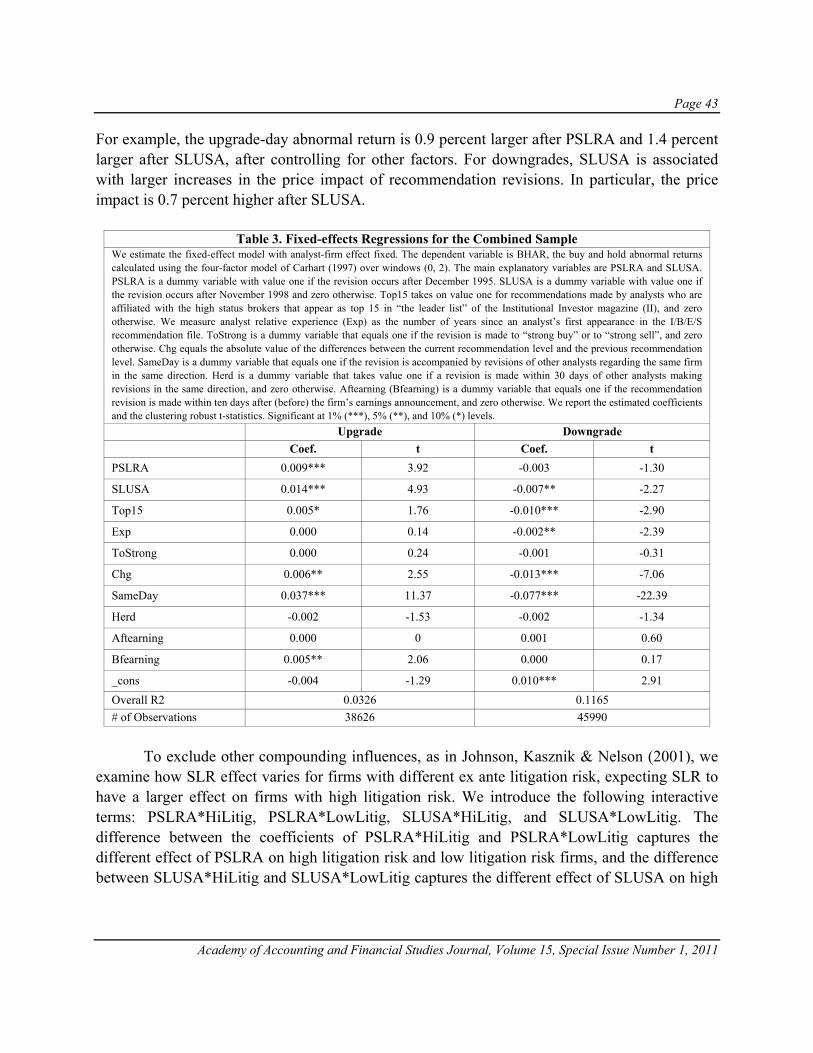
Page 43
Academy of Accounting and Financial Studies Journal, Volume 15, Special Issue Number 1, 2011
For example, the upgrade-day abnormal return is 0.9 percent larger after PSLRA and 1.4 percent larger after SLUSA, after controlling for other factors. For downgrades, SLUSA is associated with larger increases in the price impact of recommendation revisions. In particular, the price impact is 0.7 percent higher after SLUSA.
Table 3. Fixed-effects Regressions for the Combined Sample We estimate the fixed-effect model with analyst-firm effect fixed. The dependent variable is BHAR, the buy and hold abnormal returns calculated using the four-factor model of Carhart (1997) over windows (0, 2). The main explanatory variables are PSLRA and SLUSA. PSLRA is a dummy variable with value one if the revision occurs after December 1995. SLUSA is a dummy variable with value one if the revision occurs after November 1998 and zero otherwise. Top15 takes on value one for recommendations made by analysts who are affiliated with the high status brokers that appear as top 15 in “the leader list” of the Institutional Investor magazine (II), and zero otherwise. We measure analyst relative experience (Exp) as the number of years since an analyst’s first appearance in the I/B/E/S recommendation file. ToStrong is a dummy variable that equals one if the revision is made to “strong buy” or to “strong sell”, and zero otherwise. Chg equals the absolute value of the differences between the current recommendation level and the previous recommendation level. SameDay is a dummy variable that equals one if the revision is accompanied by revisions of other analysts regarding the same firm in the same direction. Herd is a dummy variable that takes value one if a revision is made within 30 days of other analysts making revisions in the same direction, and zero otherwise. Aftearning (Bfearning) is a dummy variable that equals one if the recommendation revision is made within ten days after (before) the firm’s earnings announcement, and zero otherwise. We report the estimated coefficients and the clustering robust t-statistics. Significant at 1% (***), 5% (**), and 10% (*) levels. Upgrade Downgrade Coef. t Coef. t PSLRA 0.009*** 3.92 -0.003 -1.30
SLUSA 0.014*** 4.93 -0.007** -2.27
Top15 0.005* 1.76 -0.010*** -2.90
Exp 0.000 0.14 -0.002** -2.39
ToStrong 0.000 0.24 -0.001 -0.31
Chg 0.006** 2.55 -0.013*** -7.06
SameDay 0.037*** 11.37 -0.077*** -22.39
Herd -0.002 -1.53 -0.002 -1.34
Aftearning 0.000 0 0.001 0.60
Bfearning 0.005** 2.06 0.000 0.17
_cons -0.004 -1.29 0.010*** 2.91 Overall R2 0.0326 0.1165 # of Observations 38626 45990
To exclude other compounding influences, as in Johnson, Kasznik & Nelson (2001), we examine how SLR effect varies for firms with different ex ante litigation risk, expecting SLR to have a larger effect on firms with high litigation risk. We introduce the following interactive terms: PSLRA*HiLitig, PSLRA*LowLitig, SLUSA*HiLitig, and SLUSA*LowLitig. The difference between the coefficients of PSLRA*HiLitig and PSLRA*LowLitig captures the different effect of PSLRA on high litigation risk and low litigation risk firms, and the difference between SLUSA*HiLitig and SLUSA*LowLitig captures the different effect of SLUSA on high
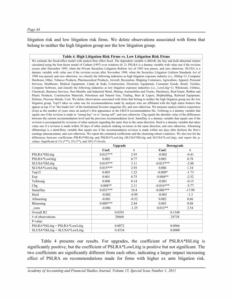
Page 44
Academy of Accounting and Financial Studies Journal, Volume 15, Special Issue Number 1, 2011
litigation risk and low litigation risk firms. We delete observations associated with firms that belong to neither the high litigation group nor the low litigation group.
Table 4. High Litigation Risk Firms vs. Low Litigation Risk Firms We estimate the fixed-effect model with analyst-firm effect fixed. The dependent variable is BHAR, the buy and hold abnormal returns calculated using the four-factor model of Carhart (1997) over windows (0, 2). PSLRA is a dummy variable with value one if the revision occurs after December 1995, when the Private Securities Litigation Reform Act of 1995 was passes, and zero otherwise. SLUSA is a dummy variable with value one if the revision occurs after November 1998, when the Securities Litigation Uniform Standards Act of 1998 was passed, and zero otherwise. we classify the following industries as high litigation exposure industry (i.e., Hilitig=1): Computer Hardware, Other, Tobacco Products, Pharmaceutical Products, Aircraft, Recreation, Shipping Containers, Agriculture, Apparel, Personal Services, Healthcare, Medical Equipment, Candy & Soda, Construction, Electronic Equipment, Consumer Goods, Retail, Textiles, Computer Software, and classify the following industries as low litigation exposure industries (i.e., LowLitig=1): Wholesale, Utilities, Chemicals, Business Services, Non-Metallic and Industrial Metal, Mining, Automobiles and Trucks, Machinery, Real Estate, Rubber and Plastic Products, Construction Materials, Petroleum and Natural Gas, Trading, Beer & Liquor, Shipbuilding, Railroad Equipment, Defense, Precious Metals, Coal. We delete observations associated with firms that belong to neither the high litigation group nor the low litigation group. Top15 takes on value one for recommendations made by analysts who are affiliated with the high status brokers that appear as top 15 in “the leader list” of the Institutional Investor magazine (II), and zero otherwise. We measure analyst relative experience (Exp) as the number of years since an analyst’s first appearance in the I/B/E/S recommendation file. ToStrong is a dummy variable that equals one if the revision is made to “strong buy” or to “strong sell”, and zero otherwise. Chg equals the absolute value of the differences between the current recommendation level and the previous recommendation level. SameDay is a dummy variable that equals one if the revision is accompanied by revisions of other analysts regarding the same firm in the same direction. Herd is a dummy variable that takes value one if a revision is made within 30 days of other analysts making revisions in the same direction, and zero otherwise. Aftearning (Bfearning) is a dumLRmy variable that equals one if the recommendation revision is made within ten days after (before) the firm’s earnings announcement, and zero otherwise. We report the estimated coefficients and the clustering robust t-statistics. We also test for the differences between coefficients PSLRA*HiLitig and PSLRA*LowLitig (SLUSA*HiLitig and SLUSA*LowLitig), and report the p-values. Significant at 1% (***), 5% (**), and 10% (*) levels. Upgrade Downgrade Coef. t Coef. t PSLRA*HiLitig 0.012*** 2.93 -0.002 -0.41 PSLRA*Lowlitig 0.003 0.77 0.003 0.78 SLUSA*HiLitig 0.014*** 3.11 -0.015*** -2.88 SLUSA*LowLitig 0.015*** 2.93 0.006 1.34 Top15 0.005 1.22 -0.008* -1.73 Exp 0.001 0.75 -0.004** -2.52 ToStrong 0.000 0.14 -0.001 -0.15 Chg 0.008** 2.11 -0.016*** -5.77 SameDay 0.051*** 10.4 -0.086*** -17.99 Herd -0.002 -0.99 -0.003 -1.3 Aftearning -0.001 -0.52 0.002 0.66 Bfearning 0.009*** 2.84 0.003 0.88 _cons -0.006 -1.25 0.012** 2.54 Overall R2 0.0391 0.1348 # of observations 20660 24738 P-value PSLRA*HiLitig = PSLRA*LowLitig 0.0072 0.0966 SLUSA*HiLitig = SLUSA*LowLitig 0.4334 0.0000
Table 4 presents our results. For upgrades, the coefficient of PSLRA*HiLitig is significantly positive, but the coefficient of PSLRA*LowLitig is positive but not significant. The two coefficients are significantly different from each other, indicating a larger impact increasing effect of PSLRA on recommendations made for firms with higher ex ante litigation risk.

Page 45
Academy of Accounting and Financial Studies Journal, Volume 15, Special Issue Number 1, 2011
However, we find that the coefficients of SLUSA*HiLitig and SLUSA*LowLitig are both positive and significant, and that there is no significant difference between these two coefficients. Regarding downgrades, we document a larger price impact increasing effect of both PSLRA and SLUSA on firms with higher ex ante litigation risk. Specifically, we find that the coefficient of PSLRA*HiLitig is significantly smaller than the coefficient of PSLRA*LowLitig. That is, the increases in the impact of analyst downgrades are significantly larger for high litigation firms than for low litigation firms. For SLUSA, it is associated with significantly lower three-day abnormal returns only for high litigation firms, and the coefficient of SLUSA*HiLitig is significantly smaller than the coefficient of SLUSA*LowLitig. Overall, consistent with our hypothesis that analyst impact has increased after PSLRA, we show that firms with higher ex ante litigation risk experience larger increases in the short-term market reactions to analyst recommendation revisions following PSLRA. We document similar results for analyst downgrades following SLUSA, but we do not find significant difference for analyst upgrades before and after SLUSA, possibly because SLUSA, which closed a loophole in PSLRA, only has a secondary effect on the information environment.
CONCLUSION We examine the effect of SLR, which brings increased complexity and noisiness in the information environment by offering public companies a safe harbor for forward looking information, on analyst research impact. Using a fixed effect model with analyst-firm effect fixed, we find that SLR has a significant price-impact increasing effect on analyst recommendation revisions after controlling for recommendation-level factors and analyst experiences. To exclude compounding influences, we further show that firms with higher ex ante litigation risk generally experience larger increases in the short-term market reactions to analyst recommendation revisions following SLR. Our study highlights analysts’ role in the financial market by showing that investors rely more heavily on analyst research in the post-SLR era when information becomes more complicated and nosier, thereby requiring greater professional expertise.
ENDNOTES 1. Forbes, “Bill Lerach thinks of himself as Robin Hood in a class-action suit”, Oct 9, 1995. Pg 116 2. Institutional Investor, “Finally, a Safe Harbor”, Mar 1996, Vol. 30(3), Pg 41 3. CFO, “Ending the Cat-and- Mouse Game”, Feb. 1996, Vol. 12(11), Pg 11 4. Business Week, “Don't toss this stock-fraud law. Just fix it”, August 5, 2002, Iss. 3794, Pg 86 5. There are totally 395 revisions in these two months, while for the months remained in our sample, the
average number per month is about 1,200. 6. Cumulative abnormal returns (CAR) yield similar results.
Page 46
Academy of Accounting and Financial Studies Journal, Volume 15, Special Issue Number 1, 2011
7. The company industry information is collected from Compustat, and the data for earnings-related class action lawsuits between 1988 and 1994 are generously provided by Doug Skinner.
REFERENCES Ali, A. & S. Kallapur (2001). Securities price consequences of the Private Securities Litigation Reform Act of 1995
and related events. Accounting Review 76, 431-61. Carhart, M.M. (1997). On persistence in mutual fund performance. Journal of Finance 52, 57-82. Clement, M.B. & Tse S.Y. (2005). Financial analyst characteristics and herding behavior in forecasting. Journal of
Finance 60, 307-41 Field, L., M. Lowry & S. Shu (2005). Does disclosure deter or trigger litigation? Journal of Accounting and
Economics 39, 487-507 Gintschel, A. & S. Markov (2004). The effectiveness of Regulation FD. Journal of Accounting and Economics 37,
293-314 Grundfest, J.A. & M.A. Perino (1997). Securities litigation reform: The first year’s experience. 29th Annual Institute
on Securities Regulation, New York: Practising Law Institute, 241-295. Ivkovic, Z. & N. Jegadeesh (2004). The timing and value of forecast and recommendation revisions. Journal of
Financial Economics 73, 433-63. Johnson, M., R. Kasznik & K. Nelson (2000). Shareholder wealth effects of the Private Securities Litigation Reform
Act of 1995. Review of Accounting Studies 5, 217-33. Johnson, M., R. Kasznik & K. Nelson (2001). The impact of Securities Litigation Reform on the disclosure of
forward-looking information by high technology firms. Journal of Accounting Research 39, 297-327. Lerach, W.S. (1998). The Private Securities Litigation Reform Act of 1995-27 months later: Securities class action
litigation under The Private Securities Litigation Reform Act’s brave new world. Washington University Law Quarterly 76, 597-644.
Spiess, D.K. & P. A. Tkac (1997). The Private Securities Litigation Reform Act of 1995: The stock market casts its
vote. Managerial and Decision Economics 18, 545-61. Stickel, S.E. (1995). The anatomy of the performance of buy and sell recommendations. Financial Analyst Journal
51, 25-39.

Page 47
Academy of Accounting and Financial Studies Journal, Volume 15, Special Issue Number 1, 2011
EXCHANGE TRADED NOTES AND THE LEHMAN BANKRUPTCY
Kenneth Washer, Creighton University Randy Jorgensen, Creighton University
ABSTRACT
Exchange traded notes (ETNs) have existed since 2006 yet they have received scant attention in the academic literature. ETNs have several advantages over exchange traded funds (ETFs) such as minimal tracking error and favorable tax treatment. On the negative side, ETN investors bear credit risk, which was severe during the Great Recession. Since ETNs and ETFs are often structured based on the same indexes and are not always easily distinguishable from one another by investors, a comparison of the two types of securities is important. This study provides institutional and technical details related to ETNs that investors should understand better. The study also investigates the most significant risk affecting ETNs, credit risk, using regression analysis. The regression results show that credit risk matters as higher credit spreads decrease the number of ETNs outstanding. As a practical matter for investors, events like the Lehman bankruptcy in September 2008 will impact the demand for ETNs, which will remain volatile and subject to economic conditions.
INTRODUCTION Exchange traded notes (ETNs) allow investors to go long or short in markets that often are not readily accessible by small investors, such as commodities. The value of doing so has obvious implications for an investor seeking to diversify beyond equities and fixed income investments. ETNs were first introduced by Barclay’s Bank PLC on June 12, 2006 when it issued the iPath® Dow Jones-UBS Commodity Total Return ETN (ticker symbol DJP). By June 2009, there were 86 U.S. listed ETNs trading in financial markets. Since their introduction, they have traded alongside their close cousins, exchange traded funds (ETFs), often with little distinction made between the two. Indeed, for several years the Wall Street Journal listed the top 100 “Exchange Traded Portfolios” in a table each day. The first quote in the table was DJP, an ETN, and all other security quotes were for ETFs. There are important differences in terms of taxes, tracking error and credit risk between ETFs and ETNs and yet ETNs have largely been ignored in the academic literature. Most tellingly, the bankruptcy of Lehman Brothers and the associated impact on their notes was discussed in the popular press but went largely unnoticed in the academic arena. The goals of this study are to provide an introduction to the structural and market characteristics of ETNs and
Page 48
Academy of Accounting and Financial Studies Journal, Volume 15, Special Issue Number 1, 2011
to examine the similarities and differences between ETNs and ETFs. This study also investigates the issue of credit risk in ETNs by examining the performance of Lehman Brothers notes around the time of the firm’s bankruptcy. The paper is constructed as follows. The following section discusses the structure and characteristics of ETNs. Next, the Lehman Bankruptcy and its impact on credit risk are examined. The final two sections present an analysis of the influence acute credit risk has on ETNs, followed by a conclusions section summarizing the study.
ETNS: BACKGROUND AND STRUCTURE Shortly after Barclays first introduced ETNs, other firms quickly followed suit by creating ETNs of their own. Today, there are essentially four ETN families: iPath® (Barclays Bank), PowerShares® (Deutsche Bank AG), ELEMENTSTM (Deutsche Bank AG, Credit Suisse, and Swedish Export Credit Corporation), and E-TRACS (UBS). UBS’s E-TRACs were launched in April 2008 and all are linked to commodities with its CMCI Long Platinum ETN being the most popular issue. ELEMENTSTM ETNs are unique in that there are four separate issuers under this brand: Swedish Export Credit Corporation has 7 issues, Deutsche Bank has 10, HSBC has 1, and Credit Suisse has 4 issues. While most ETNs are linked to a single index, some offer more aggressive investment strategies. For example, two of PowerShares’ ETNs are double long an index and one is double short. ETNs have significant structural differences when compared with ETFs. In spite of what might turn out to be very meaningful differences in risks/rewards, retail investors may easily mistake ETNs for ETFs. Although Barclays has branded their ETNs with the name “iPath®” and their ETFs with “iShares®”, other issuers have not been so forthright. For example, Deutsche Bank brands both its ETNs and ETFs with the “PowerShares” name. The most important difference between ETNs and ETFs is the underlying structure, which also holds the key to why this financial innovation matters to investors. ETF shareholders actually own a claim on an underlying portfolio, which protects them in case the management company running the portfolio goes bankrupt. Alternatively, ETN investors do not own a portfolio; they simply have a general claim on the issuer’s assets if bankruptcy occurs. ETNs are essentially zero coupon, variable rate, unsecured notes that offer no principal protection and have an underlying return tied to the performance of an index. For example, Barclay’s DJP has a principal value of $50, but the subsequent value of this 30-year note is tied to the Dow Jones-UBS Commodity Index. The largest ETNs trade on stock exchanges and investors can take long or short positions. Because there is no portfolio that must be managed, an ETN is able to more closely track an index than an ETF based on the same index. An important feature of ETNs is the ability to redeem them under certain circumstances. The value of an ETN is linked to an index, so the notes should trade very close to their intrinsic value, assuming there is a deep and liquid market. If these structured notes were to sell
Page 49
Academy of Accounting and Financial Studies Journal, Volume 15, Special Issue Number 1, 2011
significantly below economic value, often called indicative value, arbitrageurs would purchase and redeem them with the issuer, capturing the discount. Alternatively, if the notes were to trade significantly above indicative value, the issuer would sell additional units. The redemption feature offers protection of value in the case of credit downgrades of the underwriting bank. As long as the redemption feature is intact and there are institutions willing to arbitrage when the market price falls below the redemption value, credit rating downgrades on the issuer will not impact the price of the notes. However, as discussed later, if the issuer goes into bankruptcy, as happened to Lehman Brothers, the value of the notes will reflect the issuer’s increased credit risk. ETNs have several advantages over ETFs. As mentioned previously, since they are not based on an underlying asset pool they allow retail investors to capture returns ETFs cannot, such as from PowerShares Crude Oil Double Long as well as their double short product. In addition, ETNs may offer higher after-tax returns than similar ETFs while at the same time offering lower tracking risk. ETN issuers recommend treating all but single currency issues as prepaid contracts for tax purposes. A prepaid contract is one where you disburse an amount today for the promise of a contingent payment in the future. No intermediate cash distributions (dividends and/or interest payments) occur, so no taxable income is reported. Taxes would only be paid when the ETN matures or when the investor sells it in the secondary market. The investor can control both the timing of the tax liability and the tax rate incurred, whether taxed as current income or capital gains, by timing purchases and sales appropriately. ETFs, on the other hand, are generally set up as regulated investment companies and must distribute annual income and capital gains to shareholders. If a taxable investor were comparing an S&P 500 Index fund to an ETN that promises to pay the total return on the S&P 500 at maturity, the note would offer significant tax benefits. With a dividend yield of 3%, the fund would pass dividends along each year to shareholders, who may then face a tax liability. Alternatively, the holder of the note would have the 3% yield included in the total return, which would be received at a later date and potentially subject to a long-term capital gains rate. The Internal Revenue Service (IRS) has yet to rule on many types of ETNs. Much of the literature produced by the issuers encourages investors to treat ETNs as prepaid contracts for tax purposes with the exception of single currency ETNs, discussed below. However, the four top issuers also recommend consulting a tax adviser. The IRS has solicited comments on the appropriate tax treatment of instruments such as commodity and equity ETNs, but has yet to rule on this issue. Velotta (2008) suggests “practitioners should be aware of the (taxation) developments as ETNs and other newly created investment products make their way more and more into the hands of the retail investor.” The IRS has ruled on single currency ETNs via Revenue Ruling 2008-1, issued on December 7, 2007. This ruling says that a debt instrument should be taxed as a debt instrument regardless of the currency of denomination. For example, the iPath® euro/US single currency

Page 50
Academy of Accounting and Financial Studies Journal, Volume 15, Special Issue Number 1, 2011
ETN is tied to the exchange rate between the euro and the dollar. When the euro decreases relative to the dollar, the indicative value of the ETN goes down. According to interest rate parity, the change in exchange rates is linked to interest rates associated with the two currencies. If euro rates are 4% over the coming year and US rates are 2%, then the euro/US currency exchange rate should decrease by 2%. The revenue ruling applies to all single currency ETNs and means that even though investors do not receive an interest payment from the euro/US ETN, they must accrue interest annually and pay tax on it. The other significant benefit of ETNs is that they have almost no tracking error. Equity and fixed income index funds often fall short of their benchmark due to transaction costs, cash drag, and/or a portfolio that is not a perfect replica of the index. The same is true for ETFs. The largest ETF is SPDR S&P 500 (ticker symbol SPY) and it has a tracking error that averaged 15 basis points per year over the period 1998-2008. According to a recent study prepared by Morgan Stanley and quoted in the Wall Street Journal (Salisbury, 2010), ETFs missed their targets by an average of 125 basis points in 2009. In addition, 54 ETFs fell short of the mark by more than three percentage points while a few missed by more than ten percentage points. Such is not the case for ETNs, even when based on similar target indexes. Tracking error is minimal for ETN investors since they receive the benchmark return minus a fixed fee. ETN issuers claim to hedge their underlying risks through futures contracts and build tracking error into the fee charged. Overall, the differences between ETFs and ETNs can lead to differences in taxability, tracking performance, and credit risk. In addition, ETNs offer a wider array of investment strategies such as the ability to invest double long or short certain indexes. It is clear structured notes play an important role in the financial markets.
Figure 1 Average daily trading volume*
Source: Bloomberg
* Calculated over a 30-day period for 86 US listed ETNs on June 15, 2009
05
101520253035
0-1k 1k-10k 10k-50k 50k-100k over 100k
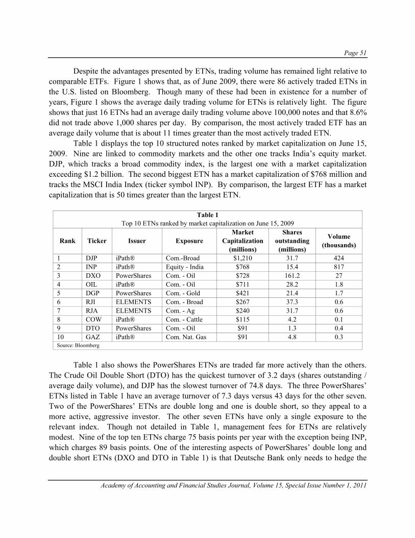
Page 51
Academy of Accounting and Financial Studies Journal, Volume 15, Special Issue Number 1, 2011
Despite the advantages presented by ETNs, trading volume has remained light relative to comparable ETFs. Figure 1 shows that, as of June 2009, there were 86 actively traded ETNs in the U.S. listed on Bloomberg. Though many of these had been in existence for a number of years, Figure 1 shows the average daily trading volume for ETNs is relatively light. The figure shows that just 16 ETNs had an average daily trading volume above 100,000 notes and that 8.6% did not trade above 1,000 shares per day. By comparison, the most actively traded ETF has an average daily volume that is about 11 times greater than the most actively traded ETN. Table 1 displays the top 10 structured notes ranked by market capitalization on June 15, 2009. Nine are linked to commodity markets and the other one tracks India’s equity market. DJP, which tracks a broad commodity index, is the largest one with a market capitalization exceeding $1.2 billion. The second biggest ETN has a market capitalization of $768 million and tracks the MSCI India Index (ticker symbol INP). By comparison, the largest ETF has a market capitalization that is 50 times greater than the largest ETN.
Table 1 Top 10 ETNs ranked by market capitalization on June 15, 2009
Rank Ticker Issuer Exposure Market
Capitalization (millions)
Shares outstanding
(millions)
Volume (thousands)
1 DJP iPath® Com.-Broad $1,210 31.7 424 2 INP iPath® Equity - India $768 15.4 817 3 DXO PowerShares Com. - Oil $728 161.2 27 4 OIL iPath® Com. - Oil $711 28.2 1.8 5 DGP PowerShares Com. - Gold $421 21.4 1.7 6 RJI ELEMENTS Com. - Broad $267 37.3 0.6 7 RJA ELEMENTS Com. - Ag $240 31.7 0.6 8 COW iPath® Com. - Cattle $115 4.2 0.1 9 DTO PowerShares Com. - Oil $91 1.3 0.4 10 GAZ iPath® Com. Nat. Gas $91 4.8 0.3 Source: Bloomberg
Table 1 also shows the PowerShares ETNs are traded far more actively than the others. The Crude Oil Double Short (DTO) has the quickest turnover of 3.2 days (shares outstanding / average daily volume), and DJP has the slowest turnover of 74.8 days. The three PowerShares’ ETNs listed in Table 1 have an average turnover of 7.3 days versus 43 days for the other seven. Two of the PowerShares’ ETNs are double long and one is double short, so they appeal to a more active, aggressive investor. The other seven ETNs have only a single exposure to the relevant index. Though not detailed in Table 1, management fees for ETNs are relatively modest. Nine of the top ten ETNs charge 75 basis points per year with the exception being INP, which charges 89 basis points. One of the interesting aspects of PowerShares’ double long and double short ETNs (DXO and DTO in Table 1) is that Deutsche Bank only needs to hedge the

Page 52
Academy of Accounting and Financial Studies Journal, Volume 15, Special Issue Number 1, 2011
net position, but is compensated based on the total. Thus, on June 9, 2009 the net exposure was $637 million ($728 – $91) long times two. However, Deutsche Bank earns the 75 basis point fee on the total of $819 million ($728 + $91). Figure 2 demonstrates the divergence between ETNs and ETFs from June 23, 2006 to June 23, 2009. The figure compares the number of outstanding DJP notes and PowerShares’ DB Commodity Index Tracking Fund shares (DBC). These two securities are based on almost identical indexes and are thus very similar except that one is structured as a note and the other as a fund. Both products had impressive growth in volume outstanding leading up to the financial crisis, although the amount outstanding for each showed a peak in mid-2008. About the time Lehman filed for bankruptcy in September 2008, investors clearly began to show a greater preference for the ETF as its shares outstanding reached new heights while the comparable ETN declined. The number of notes outstanding for the ETN has stabilized, but still remains off about 40% from its high. The next sections examine this topic in greater detail.
Figure 2 notes and shares outstanding*
Source: Bloomberg
* in millions
CREDIT RISK AND THE LEHMAN BANKRUPTCY On September 15, 2008 Lehman Brothers filed for Chapter 11 bankruptcy protection. It had over $600 billion in assets and distinguished itself as one of the largest investment banks to ever fail. The event was such a shock to financial markets that it prompted Peter G. Peterson, the co-founder of the private equity firm the Blackstone Group, to say “I’ve been in the business 35
0
20
40
60
80
100
120
140
6/28
/06
9/28
/06
12/2
8/06
3/28
/07
6/28
/07
9/28
/07
12/2
8/07
3/28
/08
6/28
/08
9/28
/08
12/2
8/08
3/28
/09
Shar
es/N
otes
Date
DJP (ETN)
DBC (ETF)

Page 53
Academy of Accounting and Financial Studies Journal, Volume 15, Special Issue Number 1, 2011
years, and these are the most extraordinary events I’ve ever seen” (Sorkin 2008). Though other banks such as Merrill Lynch also invested heavily in risky real estate and also had inadequate levels of capital, the Federal Reserve arranged for the purchase of Merrill by Bank of America, yet allowed Lehman to fail. This decision had significant consequences for ETN investors. At the time of its bankruptcy, Lehman had the following three ETNs:
1. The Opta® Lehman Brothers Commodity Pure Beta Total Return ETN (RAW), tracked a diversified commodity index and had a market capitalization of about $4.8 million prior to the filing.
2. The Opta® Lehman Brothers Commodity Pure Beta Agriculture Total Return ETN (EOH) tracked an agricultural index and had a market capitalization of about $4.4 million prior to the filing.
3. The Opta® S&P Listed Private Equity Net Return ETN (PPE) tracked a 30-component index of listed private equity companies and had a market capitalization of about $4.3 million prior to the filing.
Once Lehman went into bankruptcy, the redemption feature for its three Opta® notes was eliminated. At this point the investors became general creditors in the bankruptcy process and the notes stopped trading on the American Stock Exchange and went to the pink sheets. Interestingly, at the close of trading on Friday prior to the Monday filing, the Opta® ETNs were trading at intrinsic value. The perceived underlying credit risk was not priced into them. The holders of these ETNs ultimately lost virtually 100% of their investment. Lehman was thought by many to be too-big-to-fail, and its bankruptcy filing was shocking. Prior to this event, investors likely gave little consideration to the credit quality issues related to ETNs. In the weeks subsequent to the bankruptcy filing, one might have expected massive redemptions of ETNs issued by other companies, but this was not the case. Figure 2 shows the redemptions that occurred in DJP, the most popular ETN in terms of volume outstanding, in the week of the Lehman bankruptcy. DJP had a total of 1,135,900 notes redeemed during the week of Lehman’s bankruptcy filing, or roughly 2% of the total notes outstanding. The Figure also shows that over 20 million of these notes were redeemed in the second half of 2008. Barclays was forced to switch from a steady issuer of DJP notes to a required buyer. Although the number of notes outstanding declined in 2008, the amount issued began to grow again in 2009. Thus, it seems that although the Lehman failure demonstrated the credit risk inherent in ETNs there was likely very little contagion effect among other issues. The decline in the number of shares of DJP outstanding could be a reaction only to credit risk, however, another potential cause for redemptions of these notes was their poor returns. Commodity prices fell relatively quickly over the latter half of 2008 at the same time many investors were cashing out of risky investments. This flight to safety could explain the redemptions of DJP, however, during that same period investors continued to purchase many

Page 54
Academy of Accounting and Financial Studies Journal, Volume 15, Special Issue Number 1, 2011
new shares of DBC - the ETF alternative to DJP. These issues are addressed using regression analysis in the next section.
REGRESSION MODEL Equation 1 below is used to estimate the impact of Lehman’s bankruptcy filing on the number of notes outstanding of one ETN, DJP. DJP is used because there is an ETF that is based on the same index and is, therefore, a close substitute. The DB Commodity Index Tracking Fund is equivalent to DJP in all respects except for the structure, as it is an ETF and not an ETN. In addition, the DJP ETN has the largest number of notes outstanding thereby minimizing the potential issues associated with lightly traded securities.
ttsharesttnotes eDBCBSpreadBBDJP +Δ++=Δ )(210)( (1) where,
ΔDJPnotes(t) = The weekly change in the number of DJP notes outstanding. Spread(t) = The difference between the Bloomberg Fair Value US Global
BBB 10-year corporate rate and the comparable Treasury note rate.
ΔDBCshares(t) = The weekly change in the number of DBC shares outstanding. et = Normally distributed error term with a mean of 0 and a constant
variance. The dependent variable in the model is the number of DJP notes issued or redeemed during a trading week. Two factors are hypothesized to impact the change in the number of notes: 1) risk aversion and 2) demand for commodity investments. The proxy used for risk aversion is the difference between the Bloomberg Fair Value (BFV) US Global BBB rated 10-year note yield and the comparable 10-year US Treasury note yield. The less willing investors are to bear risk, the greater the difference between these two rates and thus the larger the spread. The null and alternative hypotheses for risk are: H0 B1 ≥ 0 Ha B1 < 0 Rejecting the null in this case implies that an increase (decrease) in the credit spread leads to a decrease (increase) in ETNs. The demand for DJP notes may also be affected by investor appetite for commodity investments. The change in the shares outstanding of a comparable commodity investment that
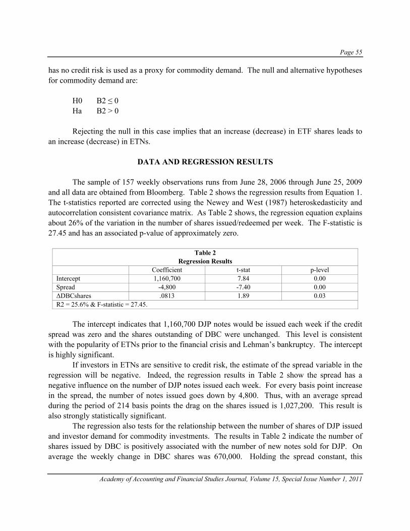
Page 55
Academy of Accounting and Financial Studies Journal, Volume 15, Special Issue Number 1, 2011
has no credit risk is used as a proxy for commodity demand. The null and alternative hypotheses for commodity demand are: H0 B2 ≤ 0 Ha B2 > 0 Rejecting the null in this case implies that an increase (decrease) in ETF shares leads to an increase (decrease) in ETNs.
DATA AND REGRESSION RESULTS The sample of 157 weekly observations runs from June 28, 2006 through June 25, 2009 and all data are obtained from Bloomberg. Table 2 shows the regression results from Equation 1. The t-statistics reported are corrected using the Newey and West (1987) heteroskedasticity and autocorrelation consistent covariance matrix. As Table 2 shows, the regression equation explains about 26% of the variation in the number of shares issued/redeemed per week. The F-statistic is 27.45 and has an associated p-value of approximately zero.
Table 2 Regression Results
Coefficient t-stat p-level Intercept 1,160,700 7.84 0.00 Spread -4,800 -7.40 0.00 ΔDBCshares .0813 1.89 0.03 R2 = 25.6% & F-statistic = 27.45.
The intercept indicates that 1,160,700 DJP notes would be issued each week if the credit spread was zero and the shares outstanding of DBC were unchanged. This level is consistent with the popularity of ETNs prior to the financial crisis and Lehman’s bankruptcy. The intercept is highly significant. If investors in ETNs are sensitive to credit risk, the estimate of the spread variable in the regression will be negative. Indeed, the regression results in Table 2 show the spread has a negative influence on the number of DJP notes issued each week. For every basis point increase in the spread, the number of notes issued goes down by 4,800. Thus, with an average spread during the period of 214 basis points the drag on the shares issued is 1,027,200. This result is also strongly statistically significant. The regression also tests for the relationship between the number of shares of DJP issued and investor demand for commodity investments. The results in Table 2 indicate the number of shares issued by DBC is positively associated with the number of new notes sold for DJP. On average the weekly change in DBC shares was 670,000. Holding the spread constant, this
Page 56
Academy of Accounting and Financial Studies Journal, Volume 15, Special Issue Number 1, 2011
coefficient of 0.0813 translates into 54,471 notes of DJP issued. Again, the result is strongly statistically significant. The regression results indicate that the demand for DJP notes is positively related to demand for commodity investments as expected. In addition, the demand for this particular ETN is negatively related to investor credit risk aversion. A visual examination of Figure 2 reveals that, prior to the Lehman bankruptcy, investor risk aversion appeared to play a slight role in the demand for these notes. It is equally clear that after the Lehman bankruptcy, and as investors became more credit risk averse, the demand for this ETN declined in spite of an increased appetite for commodity investments. Taken together, these results show that the demand for this particular ETN is sensitive to credit risk and that ETFs act as a substitute for ETNs during such periods. These results suggest that future demand for ETNs will be uneven and pro-cyclical. This is problematic for issuing banks such as Barclays because during downturns they often need to conserve equity capital to stay solvent. ETN holders put pressure on these banks as they redeem notes causing the banks to use up precious capital or get expensive external funding. There are two primary ways issuers can avoid the massive redemptions of ETNs during times of economic hardship. First, they could purchase a third party guaranty from a financially strong insurer. Alternatively, the industry or government could create an institution similar to the Federal Deposit Insurance Corporation that collects fees from the issuing banks and protects investors when default occurs.
CONCLUSIONS This study explores the characteristics of exchange traded notes (ETNs), a topic that has largely been ignored in the academic literature despite the growth in importance of this market since its creation in 2006. Exchange traded notes possess advantages over equivalently-based exchange traded funds (ETFs) such as lower tracking error, tax advantages and access to more advanced investment strategies such as the ability to go double long or double short an index. The primary disadvantage of ETNs over ETFs is the existence of credit risk. Surprisingly, this study shows that credit risk was largely ignored prior to the bankruptcy of Lehman Brothers. Regression and graphical results show the Lehman Brothers bankruptcy and the large increase in credit risk spreads significantly reduced the demand for ETNs. Many investors switched to ETFs, which are good substitutes for ETNs, in order to avoid default risk. Exchange traded notes will likely never be as popular as exchange traded funds due to the credit risk involved. However, ETNs will most likely continue to be traded by investors who stress the importance of tracking performance or who are interested in the double-long or short features. Regardless, investors should be aware or, indeed, be made aware of the credit risk inherent in these securities.

Page 57
Academy of Accounting and Financial Studies Journal, Volume 15, Special Issue Number 1, 2011
REFERENCES Fletcher, J. (2009). Currency exchange traded notes (ETNs). Global Pensions 11. Fuhr, D., & Kelly, S. (2009). Contrasting the development of ETF markets. Global Pensions 21. Macchia, D. (2008). Challenges Ahead For EIAs and Structured Products. National Underwriter Life & Health
112(27), 12-13. Martin, N. A. (2008). How to Avoid the Worst of a Market Squall. Barron's. 88(14), L16, L19. Newey, W and K. West, A Simple Positive Semi-Definite Hetroskedasticity and Autocorrelation Consistent
Covariance Matrix. Exonometrica (1987) 55, pp. 703-708. Pengelly, M. (2009). The End for ETNs? Risk. 22(4), 28-30. Revenue Ruling 2008-1, Treatment of Certain Foreign Currency Transactions. www.irs.gov/pub/irs-irbs/irb08-
01.pdf. Salisbury, I. (2010). ETFs Were Wider Off the Mark in 2009. Wall Street Journal. (19 February) Sorkin, A. R. (2008). Lehman Files for Bankruptcy; Merrill is Sold. New York Times (15 September). Stinespring, J. R., & Kench, B. T. (2009). Explaining the Interbank Loan Crisis of 2008: A Teaching Note. Journal
of Economics & Economic Education Research. 10(2), 3-15. Sullivan, T. (2007). The Newest Kids in Town. Barron's. 87(1), 28-29. Velotta, R. A. (2008). Taxation of Exchange Traded Notes. Tax Adviser. 39 (8), 497-499.

Page 58
Academy of Accounting and Financial Studies Journal, Volume 15, Special Issue Number 1, 2011
Page 59
Academy of Accounting and Financial Studies Journal, Volume 15, Special Issue Number 1, 2011
MARKET IMPLICATION OF HUMAN CAPITAL INVESTMENT IN TRAINING
Chih-Hsien Liao, National Taiwan University
Songtao Mo, Purdue University Calumet Julia Grant, Case Western Reserve University
ABSTRACT
The empirical determination of whether human capital investment creates intangible assets and contributes to firms’ profitability and market values is seriously hampered by the lack of publicly disclosed information on such practices. Using unique survey data regarding employee training practices, we examine and find that employee training expenditures are positively related to both contemporaneous and future operating performance, as well as to market values. Further, following the balanced scorecard theory, we test whether incorporating training into the firm’s performance measurement system has a positive effect on firm value. The empirical results suggest that training in conjunction with the use of non-financial performance metrics (from customer, internal process, and learning and growth perspectives) is positively related to the use of performance metrics in the financial perspective, which in turn has a positive effect on firms’ market values. The establishment of a direct relationship between market price and human capital investment sheds light on corporations’ human resource management practices. This attempt integrates empirical financial accounting research with general management research, broadening the horizon for accounting scholars with regard to the significance of such internally-developed intangibles.
INTRODUCTION Intangible assets of major publicly held corporations are recognized as important determinants of firm value and economic prosperity. However, there are significant concerns about the deficiencies of information in corporate financial reports and inadequate treatment of these assets under traditional accounting principles (Lev, 2001). The failure of financial statements to fully recognize these intangibles leads to an increasing gap between firms’ market values and book values. Many studies attribute this gap to the omitted value of what they call intellectual capital (e.g., Stewart, 1994; Roos et al., 1998). Some examples include employee competence, brand names, supplier relationships, production process, and organizational culture. Although there is no consensus on everything that contributes to intellectual capital, the human capital embedded in employee competence is one of the core components agreed upon by many researchers (e.g., Brooking, 1996; Edvinsson and Malone, 1997; Roos and Roos, 1997).
Page 60
Academy of Accounting and Financial Studies Journal, Volume 15, Special Issue Number 1, 2011
According to Blundell et al. (1999), human capital is generated when an individual or a firm decides to invest resources in the development of people who work in the business. This decision is not essentially different from other investment decisions. Similar to other investment choices, human capital investment is intended to generate higher returns. In today’s technology-dependent global economy, knowledge and competence of employees become the most important sources of firms’ competitive advantages (Drucker, 1999). In fact, the concept of human capital originated in the 1960s, when economists focused on the economic benefits from investments in education and training. Investments in human capital have been shown to explain a country’s economic growth (e.g., Psacharopoulos, 1973), an individual’s earnings growth (e.g., Becker, 1964) and a firm’s employee productivity (e.g., Bartel, 1994). Researchers in the management field are also concerned about the use of human resource practices and their impact on organizational performance. Studies document that a human resource system focused on human capital enhancement is directly related to multiple dimensions of firms’ operational performance, such as employee productivity, machine efficiency and customer satisfaction (e.g., Youndt et al., 1996). There is also evidence supporting a significantly positive relationship between human capital investments and corporate financial performance, using both accounting-based measures such as return on assets and market-based measures such as Tobin’s q (e.g., Huselid, 1995). Accounting research in the 1970s mainly focused on establishing techniques in measuring the cost and value of employees (e.g., Flamholz, 1974; Friedman and Lev, 1974). Although there is some evidence of differential decision-making effect on investors (e.g., Elias, 1972; Hendricks, 1976), the failure to achieve a consensus about the measurement and reporting methods impeded further development of issues related to human capital accounting. A recent paper by Amir and Livne (2005) uses a sample of football companies in the U.K. to examine the relationship between investment in player contracts and future economic benefits, and documents that the capital market values investment in player contracts, even though the economic benefits of the contracts last no more than two years. The purpose of this paper is to assess the economic benefits as well as the valuation effect of a specific type of human capital investment—employee training. Investment in human capital can be broadly categorized into investment in employee skills and investment in employee motivation (Huselid, 1995). The former includes practices such as personnel selection, job design and employee training, which are intended to enhance employee’s knowledge, skills and abilities; the latter includes practices such as performance appraisals, promotion systems and incentive compensation, which are designed to recognize and reinforce desired employee behaviors. We focus on employee training because it is a major part of a firm’s investment in human capital following the hiring decision itself (Douthat, 1970). The value of training is not restricted solely to the employee's individual benefit. Case studies reviewed by Bartel (2000) suggest that employer’s returns on investments in training are substantial and higher than those presented in prior studies. Ballot (2006) indicates that both employees and firms benefit from

Page 61
Academy of Accounting and Financial Studies Journal, Volume 15, Special Issue Number 1, 2011
job-related trainings. Firms are motivated to provide training to enhance productivity while the employees receiving training may be compensated by future salary increase. This study advances on the research by Ballot (2006) and investigates whether firms investing in training, as a means of productivity improvement, are valued by the market. Under current U.S. accounting standards, financial statements do not recognize human capital as assets, nor do companies disclose separately their human-capital-related expenditures; therefore it has been difficult to examine whether training investment does increase firms’ operating performance and whether the capital markets can recognize this benefit. We apply a comprehensive approach to test the association between market valuation and employee training. Our study differs from previous research in that we incorporate both quantitative and qualitative aspects of training. While prior studies have demonstrated a performance effect of training, they have measured training in the form of the existence of formal training programs (e.g., Bartel, 1994), the types of training (e.g., Black and Lynch, 1996), or the number of training hours received by employees (e.g., Huselid, 1995). All of these measures are related to the costs of training, but none measure the resources invested. We consider the costs of training to be an important but missing measure because training is a consumption of firm resources, and cost-benefit analysis should be conducted in making the investment decision. Having identified a heretofore unexplored data source, we attempt to examine whether training expenditures indeed provide (future) economic benefits and are valued by the capital market. While a few studies use aggregated labor costs data to document the market valuation and performance impacts of human capital (e.g., Ballester et al., 2002; Lajili and Zeghal, 2006), such an approach aggregates uses of resources for hiring and compensation, as well as for training. This study adds to our understanding of how markets respond to investments in training. In addition, we adopt the Balanced Scorecard (BSC hereafter) framework developed by Kaplan and Norton (1992, 1996) to further examine the valuation effect of the combined use of training practices and business metrics. The human resources literature argues for the idea of internal fit, or an alignment of human resource practices with organizational strategy and performance measurement system (e.g., Huselid and Becker, 1997). A similar concept is also proposed by Kaplan and Norton (1992, 1996), who advocate the use of a balanced performance system through which to translate the firm’s strategy into action. The purpose of the BSC is to improve a firm’s external financial performance through improvement of internal non-financial performance, including customer relationships, internal process, and learning and growth. Among the four dimensions, learning and growth is the foundation, primarily represented by what employees achieve. Improved employee performance will lead to better performance in the other business areas. When a firm not only invests in employee training but also tracks and ties its training performance with both internal and external performance metrics, it is expected to increase shareholder value via the causal link between the non-financial and financial perspectives documented by the BSC literature (e.g., Cohen et al., 2006). We examine this conjecture using both qualitative and quantitative information associated with training.
Page 62
Academy of Accounting and Financial Studies Journal, Volume 15, Special Issue Number 1, 2011
The training data used in this study is obtained from the 2003-2006 Training Top 100 survey reports published by Training magazine, which ranks 100 companies for their workplace development and employee training initiatives in the previous year. We focus on public companies to document a significantly positive relationship between training expenditures and both contemporaneous and future operating performance, confirming prior evidence (using other types of data) regarding the performance effect of human capital investment. We then examine the valuation effect of training expenditures on the basis of the Ohlson (1995) model and find that training expenditures are positively associated with market values, suggesting that information about training expenditures is value relevant to investors, incremental to book value and net income. To test the effect of linking training practices to performance measures, we use factor analysis to extract factors from the various business metrics reported in the Training magazine and the results are consistent with the four perspectives in the BSC framework. We use the factor scores to measure a firm’s use of BSC in conjunction with training, and find that the combination of training and each non-financial (customer, internal process and learning and growth) perspective has an indirect and positive effect on market value. The results support the theoretical balanced scorecard argument that firms can create shareholder value by improving internal performance, which in turn increases financial performance to be valued by the capital market. Our study contributes to the literature in a number of ways. First, this study is one of the first to directly examine the capital market effect of firms’ employee training investments. Although links between other measures for human capital and organizational performance have been established, limited empirical evidence exists regarding whether employee training provides valuation-relevant information to the investors. Second, our study extends the prior stream of research on intangibles to demonstrate that employee training, like R&D and advertising, has future economic benefits that are valued positively by the capital market even though these costs are expensed immediately under accounting rules. Third, we apply an empirical methodology based on the combination of financial statement and market data with other data by directly building the connection between capital market factors and human capital investment factors. This approach is an attempt to extend accounting research into other management domains, which have not been extensively explored in accounting empirical studies. Fourth, through the examination of the valuation effect of training-related performance measurement systems, we integrate managerial accounting research with market-based accounting literature and demonstrate a linkage between information used internally and information reported externally. Our findings also have practical implications for companies in designing and implementing human resource management practices. The remainder of the paper is organized as follows. The next section reviews prior literature and develops the research hypotheses. Section three describes our data and sample. Empirical tests are analyzed in section four and robustness tests are performed in section five. Section six concludes the paper and discusses implications for future research.
Page 63
Academy of Accounting and Financial Studies Journal, Volume 15, Special Issue Number 1, 2011
LITERATURE REVIEW AND RESEARCH HYPOTHESES Human Capital Theory The theory of human capital was first elaborated by economist Mincer (1958), who demonstrated that human capital investment such as training is a primary source of earnings differentials among individuals and that investment in people should serve as the underlying principle in the analysis of income distributions. Schultz (1961) proposes that human beings and their skills and knowledge are a form of capital and that human capital has been increasing at a rate greater than nonhuman or physical capital. Becker (1962) defines investing in human capital as activities that influence future real income through the imbedding of resources in people, and he shows that trained workers are less likely to leave the employer, suggesting that training can be a mechanism to retain employees. A body of literature has examined the impact of human capital on economic growth at the macro level and on productivity at the firm level. Chuang’s (2000) analysis for Taiwan over the period 1952-1995 shows that human capital accumulation stimulates the country’s exports and fosters economic growth. Conducting a cross-sectional study of 21 Organizations for Economic Co-operation and Development (OECD) countries, Frantzen (2000) finds that both the level and growth rate of human capital positively affect a nation’s productivity growth. Zucker et al. (1998) demonstrate that the intellectual human capital of “star” scientists measured in terms of their research productivity contributed positively to the founding of U.S. biotechnology firms during the period 1976-1989. Corvers (1997) analyzes the manufacturing sectors in seven member states of the European Union and concludes that the input of human capital, measured by the proportion of intermediate and highly-skilled workers in the workforce, is positively related to the sector’s labor productivity. Other studies, using survey data about individual firm’s training programs, also document a significantly positive effect of employer-provided training on business productivity (Bartel, 1994; Black and Lynch, 1996). Researchers in the management field are another group interested in human capital. These scholars are mainly concerned about the use of human resource practices and their impact on organizational performance as well as on management decisions regarding personnel policies. They conclude that effective management of human capital creates a source of sustained competitive advantage since employee skills and commitments are key components in the value creation process (Pfeffer, 1994; Schuler, 1992; Snell and Dean, 1992; Wright and McMahan, 1992). Studies have found that effective human resource management practices such as investments in specialized management systems are associated with lower employee turnover, greater productivity and financial performance (Cascio, 1991; Huselid, 1995; Delantey and Huselid, 1996). Using a sample of 62 stores in the retail industry, Russell et al. (1985) find that the percentage of sales personnel trained is highly correlated with store performance. Bouillon, Doran and Orazem (1995) also document a significant and positive relationship between a proxy
Page 64
Academy of Accounting and Financial Studies Journal, Volume 15, Special Issue Number 1, 2011
for firm investment in specific human capital (measured as ten-year average retention rate and CEO tenure) and long-term return on assets. From the foregoing discussion, there is evidence of a positive link between human capital and organizational performance. However, none of the above studies specifically examine investment measured as actual training costs. The scope of human capital is broad, encompassing many elements. Firms do invest in human capital in various ways, such as recruiting, training, and compensation systems. According to Bontis and Fitz-enz (2002), who use survey data of 76 senior executives from 25 financial service companies to study the elements of effective human capital development, the amount spent on training is shown to be the primary measure for the human capital investment construct. They also suggest that the benefits of human capital investment should last for a long time, arguing the need for a leading indicator of firms’ future financial performance. While Bontis and Fitz-enz (2002) employ the structural equation model to develop a causal map of human capital antecedents and consequents, they do not test this argument using empirical methods on a diverse sample. We consider training as a process that requires consumption of tangible resources to generate intangible benefits, and accordingly hypothesize that:
H1.1: A firm’s employee training investment is positively related to its contemporaneous operating performance. H1.2: A firm’s employee training investment is positively related to its future operating performance.
Accounting scholars, on the other hand, intend to explain how the contributions of employees add to the value of the firm. Brummet et al. (1968) put forth the earliest work in the area of human resource measurement, advocating the use of Human Resource Accounting (HRA) information for internal planning and control purposes. The American Accounting Association (AAA) also established committees on HRA in 1972 and 1973 and published reports on the development and issues of HRA (AAA, 1973, 1974). Thereafter, a stream of research has focused on developing methods of measuring the cost and value of human resources and providing a quantitative basis for decision-making by managers as well as investors (e.g., Flamholtz, 1971, 1974; Lau and Lau, 1978; Lev and Schwartz, 1971; Morse, 1973). In spite of high interest in the attempt to value the contribution of employees, failure to establish a valid and reliable means for measuring human capital in monetary terms led to slow and inconclusive progress in this area. The discussion of human resources measurement and the debate over accounting treatment of human capital investment ebbed in the late 1970s. A few research papers address the link between human capital and its capital market impact. Using experimental settings, Ellias (1972) and Hendricks (1976) find that stock investment decisions would be different when human resource accounting information is added to conventional financial statements. However, they did not address whether the market interprets this information positively. More recently, two studies examine a sample of U.S. firms
Page 65
Academy of Accounting and Financial Studies Journal, Volume 15, Special Issue Number 1, 2011
that voluntarily disclose labor-related expenses in Compustat. Ballester et al. (2002) show that about 16 percent of such labor costs are valued by the market as investment in human capital asset whereas the rest of such costs represent an expense. Lajili and Zeghal (2006), employing a portfolio approach, find that firms disclosing labor costs and firms with higher labor productivity and efficiency indicators (estimated from a general production function) outperform their counterparts, i.e., enjoy higher abnormal returns. While the findings of Ballester et al. (2002) and Lajili and Zeghal (2006) indicate that voluntarily disclosed labor costs are perceived as value-enhancing by investors, how the market values individual components deserves further investigation. Chen et al. (2003) use the VAIC (Value Added Intellectual Coefficient) measure developed by Pulic (2000a, b) to study the relationship between intellectual capital and corporate financial performance as well as market-to-book ratios for a sample of Taiwanese firms, and their results show that companies with higher human capital efficiency have higher market-to-book ratios and greater financial performance. However, their study also uses total expenditure on employees as a proxy for firms’ human capital investment, which does not distinguish the effects of various human-capital-related components. Using a sample of 58 football companies in the U.K., Amir and Livne (2005) examine whether investment in player contracts warrants capitalization required by current accounting standards in the U.K. They find that investment in football player contracts is positively associated with firms’ future economic benefits for at most two years and that the capitalized amount of this investment is positively related to firms’ market values. Given that investments by firms in the form of training costs constitute an important part of human capital investment, this study extends prior studies by looking specifically at the market valuation of employee training. The empirical evidence regarding the relationship between employee training and firm value is lacking in the U.S., primarily because of the deficiency of required disclosures of such information in reports filed by public companies. Current U.S. accounting standards require that employee-related expenditures be expensed immediately. There is a rising debate about whether this treatment is appropriate when the importance of human capital is increasing in today’s knowledge-based economy (Lev, 2001). Following prior literature, if training enhances employees’ skills and competence to perform their jobs, firms that invest heavily in employee training are expected to have better financial performance, which in turn should affect market values. Accordingly, we expect that information about training investment will be value relevant to investors in making their investment decisions. Our second hypothesis is as follows:
H2: A firm’s employee training investment is positively related to its market value.
Page 66
Academy of Accounting and Financial Studies Journal, Volume 15, Special Issue Number 1, 2011
The Balanced Scorecard perspective Most of the literature analyzes the performance effect of human capital at the organizational level, with financial and accounting based measures of performance. Some researchers in the field of human resource management advocate a more comprehensive perspective with emphasis on performance outcomes that reflect employee attitudes and behavior, internal performance such as production output and quality, and external indicators such as sales and financial performance (Guest et al., 2000). This approach justifies the use of multiple measures of performance, both financial and non-financial, and is generally consistent with the BSC concept proposed by accounting scholars Kaplan and Norton (1992, 1993). The BSC is a performance measurement system developed by Kaplan and Norton in 1992. In addition to traditional financial measures of performance, the BSC system incorporates non-financial performance measures in three dimensions—the customer perspective, the internal perspective and the learning and growth perspective. Rooted in the organization’s overall objectives, the BSC is intended to provide strategic measurement to focus on the firm’s vision of development (Kaplan and Norton, 1993). Linked to multiple organizational behaviors, the BSC identifies factors that influence intangibles in a greater magnitude. Kaplan and Norton (2001) mention that intangibles should be examined within the organizational context, since “the value-creation related to intangibles is normally achieved by their combination with other intangible or tangible assets”. Accordingly, consideration of the qualitative characteristics of training will present a more comprehensive analysis of the association between market value and human capital investment in training. A number of studies have provided evidence that firms that align human resource practices with organizational strategy report higher performance outcomes (e.g., Huselid, 1995; Youndt et al., 1996). If BSC is designed to link all performance metrics with organizational strategy, firms that link their training practices with these measures are expected to generate more beneficial outcomes. According to the BSC framework, an improvement in the learning and growth perspective enhances the internal process and customer perspectives, which in turn improve the financial perspective. A few empirical studies have provided evidence in support of this interrelation between non-financial and financial performance (e.g., Cohen et al., 2006). However, previous literature in general only examines the effect of BSC adoption on firms’ operating performance without considering the associated capital market effect. Since the BSC is an internal management device, information about BSC usage and the various non-financial performance measures are generally not publicly available. If firms adopt and implement the BSC successfully, they will increase shareholder value through better financial performance such as revenues and profitability. Therefore, we expect that when a firm’s training practices are built into its performance measurement system consistent with the BSC framework, the effect associated with the non-financial perspectives (i.e., customer, internal process, learning and growth) will have an indirect relationship with the firm’s market value, via the effect associated

Page 67
Academy of Accounting and Financial Studies Journal, Volume 15, Special Issue Number 1, 2011
with the financial perspective. This causal relationship is demonstrated in Figure 1, according to which we develop a third set of related hypotheses:
H3.1: Firms that link training to non-financial performance measures also link training to financial performance measures. H3.2: Firms that link training to financial performance measures have higher market value.
Figure 1 The Link between Balanced Scorecard and Shareholder Value
Market Value
Balanced Scorecard
H 3.1
H 3.2
Customer Perspective
Training Internal Process Perspective
Learning and Growth
Perspective
Financial PerspectiveTraining

Page 68
Academy of Accounting and Financial Studies Journal, Volume 15, Special Issue Number 1, 2011
DATA, SAMPLE AND DESCRIPTIVE STATISTICS Data and Sample We obtain training information from the Training Top 100 survey report published by the Training magazine from year 2003 to 2006. The Training magazine has been dedicated to promoting job-related, employer-sponsored training and education in the working environment. Each year, the magazine selects and ranks one hundred companies for their workplace development and employee training initiatives in the previous fiscal year. The selection procedure is conducted through a multi-tiered process. Participating companies may be nominated by their peers, employees or training suppliers, or voluntarily apply to be considered for the Top 100, or simply respond to the mass mailings targeted at Training magazine’s circulation base. All participants answered a detailed questionnaire providing both quantitative and qualitative data; the former is evaluated using a point-based scale, and the latter is evaluated by conducting follow-up interviews. In addition to annual training expenditures (not always disclosed either for this ranking or publicly in other ways), the survey also reports whether certain business metrics of the firm are tracked and tied to training. These metrics include: retention, new employee referral, turnover, quality, productivity, customer service, customer loyalty, product development, revenue and market share. In order to obtain financial and market data, we focus on publicly-traded companies, excluding 208 observations among the 400 firm-years available. Among the 192 observations, 97 have disclosed training expenditures data, representing 49 unique firms. Ballester et al. (2002) examine the determinants of firms’ voluntary disclosure of labor-related costs, and find that disclosing firms are larger, more profitable, more labor-intensive, and tend to operate in regulated industries. Since only about 50% of the public firms in the ranking report publicly disclose their training costs, we follow Ballester et al. (2002) to see if these firms exhibit the characteristics documented in their findings. After performing t-tests of differences in means, we find that disclosing firms are not significantly different from the non-disclosing firms in the survey. Based on the findings of Ballester et al. (2002), we examine the following four characteristics: size (measured by natural logarithm of total assets), profitability (measured by return on equity), labor-intensity (measured by revenues per employee), and industry regulation (measured by a dummy variable that equals 1 if the firm revenues per employee), and industry regulation (measured by a dummy variable that equals 1 if the firm belongs to the two-digit SIC industries 40, 46, 48, 49, and 60-64, and 0 otherwise). We also perform the Heckman procedure as a sensitivity analysis to address the potential self-selection problem. We obtain the disclosing firms’ financial statement information from Compustat and stock return data from CRSP, and exclude those with missing values in these datasets. The final sample consists of 93 observations with 46 unique firms. Table 1 shows the sample distribution

Page 69
Academy of Accounting and Financial Studies Journal, Volume 15, Special Issue Number 1, 2011
by years (Panel A) and by industry (Panel B). The industries that dominate the sample are: banking and insurance (26.09%) and machinery, computer hardware and electronics (19.57%).
Table 1 Sample Distribution by Years and IndustriesPanel A: Number of firms per year
Fiscal year Number of firms 2002 242003 222004 222005 25Total 93
Panel B: Industry compositionIndustry (2-digit SIC codes) Number of firms % of totalFurniture and printing (25, 27) 2 4.35%Chemicals (28) 1 2.17%Machinery, computer hardware and electronics (35, 36) 9 19.57%Vehicles and instruments (37-39) 5 10.87%Transportation and communications (42, 45, 48) 4 8.69%Utilities (49) 1 2.17%Retail (59) 2 4.35%Banking and insurance (60-63) 12 26.09%Real estate (67) 2 4.35%Computer software (73) 5 10.87%Services (79, 87) 3 6.52%Total 46 100.00%
Descriptive Statistics
Table 2 Descriptive Statistics for Sample FirmsVariable1 N2 Mean Std Dev Q1 Median Q3
TRAINING 93 102.10 170.32 6.10 33.00 102.40NE 93 62.84 81.86 8.85 26.00 85.00TRAIN NE 93 0.0016 0.0013 0.0005 0.0010 0.0025SALES 93 19,789 24,426 2,433 9,648 30,141OI 93 3,242 4,334 249 1,366 3,977NI 93 1,819 2,459 135 795 2,398TA 93 69,525 117,165 3,539 25,554 77,317BV 93 13,151 16,634 1,386 6,394 20,186MV 93 35,250 45,781 3,482 16,593 39,134RET 93 0.1870 0.3447 0.0001 0.1386 0.30081 Except that NE is in thousands, all other variables are in million dollars 2 Number of observations over fiscal years 2002-2005 TRAINING = training expenditures (reported by Training magazine) NE = number of employees in thousands (from Compustat) TRAIN_NE = training expenditures per employee (calculated as TRAINING/1,000*NE) SALES = net sales (from Compustat) OI = operating income after depreciation (from Compustat) NI = net income before extraordinary items (from Compustat) TA = total assets (from Compustat) MV = market value of equity at fiscal year end (calculated from Compustat) BV = book value of equity (from Compustat) RET = annual stock return, calculated for the period from nine months before to three months after the end of fiscal year t (from CRSP)
Table 2 provides the descriptive statistics for the sample. During reported years 2002-2005, the average amount spent on employee training is $102 million, ranging from $1.1 million to $825 million. The sample firms have a mean (median) of 63,000 (26,000) number of
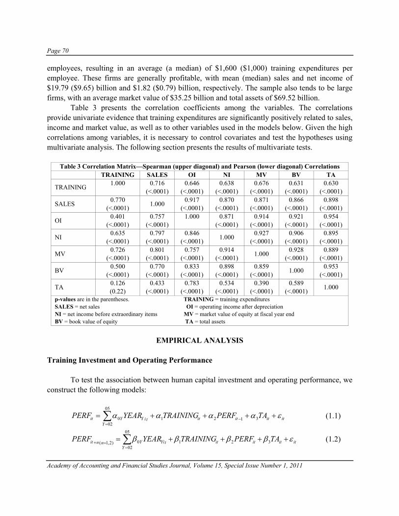
Page 70
Academy of Accounting and Financial Studies Journal, Volume 15, Special Issue Number 1, 2011
employees, resulting in an average (a median) of $1,600 ($1,000) training expenditures per employee. These firms are generally profitable, with mean (median) sales and net income of $19.79 ($9.65) billion and $1.82 ($0.79) billion, respectively. The sample also tends to be large firms, with an average market value of $35.25 billion and total assets of $69.52 billion. Table 3 presents the correlation coefficients among the variables. The correlations provide univariate evidence that training expenditures are significantly positively related to sales, income and market value, as well as to other variables used in the models below. Given the high correlations among variables, it is necessary to control covariates and test the hypotheses using multivariate analysis. The following section presents the results of multivariate tests.
Table 3 Correlation Matrix—Spearman (upper diagonal) and Pearson (lower diagonal) Correlations TRAINING SALES OI NI MV BV TA
TRAINING 1.000
0.716 (<.0001)
0.646 (<.0001)
0.638 (<.0001)
0.676 (<.0001)
0.631 (<.0001)
0.630 (<.0001)
SALES 0.770 (<.0001) 1.000 0.917
(<.0001) 0.870
(<.0001) 0.871
(<.0001) 0.866
(<.0001) 0.898
(<.0001)
OI 0.401 (<.0001)
0.757 (<.0001)
1.000
0.871 (<.0001)
0.914 (<.0001)
0.921 (<.0001)
0.954 (<.0001)
NI 0.635 (<.0001)
0.797 (<.0001)
0.846 (<.0001) 1.000 0.927
(<.0001) 0.906
(<.0001) 0.895
(<.0001)
MV 0.726 (<.0001)
0.801 (<.0001)
0.757 (<.0001)
0.914 (<.0001) 1.000 0.928
(<.0001) 0.889
(<.0001)
BV 0.500 (<.0001)
0.770 (<.0001)
0.833 (<.0001)
0.898 (<.0001)
0.859 (<.0001) 1.000 0.953
(<.0001)
TA 0.126 (0.22)
0.433 (<.0001)
0.783 (<.0001)
0.534 (<.0001)
0.390 (<.0001)
0.589 (<.0001) 1.000
p-values are in the parentheses. TRAINING = training expenditures SALES = net sales OI = operating income after depreciation NI = net income before extraordinary items MV = market value of equity at fiscal year end BV = book value of equity TA = total assets
EMPIRICAL ANALYSIS
Training Investment and Operating Performance To test the association between human capital investment and operating performance, we construct the following models:
∑=
− ++++=05
0231210
YitititittiYYit TAPERFTRAININGYEARPERF εαααα (1.1)
∑=
=+ ++++=05
023210)2,1(
YitititittYiYnnit TAPERFTRAININGYEARPERF εββββ (1.2)

Page 71
Academy of Accounting and Financial Studies Journal, Volume 15, Special Issue Number 1, 2011
where PERF is measured by operating income. We permit the regression intercept to vary across years to control for time-specific effects, represented by the indicator YEAR. TRAINING denotes the amount of training expenditures. We also control for lagged performance and size (measured by total assets, TA). Controlling performance in the prior year reflects a Granger-type lead-lag relation, since better performance gives the firm more resources to invest in training which in turn improves future performance. Equation (1.1) estimates the relation between training and contemporaneous operating performance. Equation (1.2) estimates the relation between training and both one-year-ahead and two-year-ahead operating performance, i.e., this formulation takes into account the fact that the benefits of training may lag the investments. According to the research hypotheses, we expect α1 and β1 to be positive. We deflate all variables by number of employees and estimate the model using Ordinary Least Squares (OLS).
Table 4 The Association between Training and Operating Performance Panel A: Contemporaneous Effect
∑=
− ++++=05
0231210
tititititttit TAPERFTRAININGYEARPERF εαααα (1.1)
Variable1 Predicted Sign PERFt TRAININGt + 2.30 (1.40)* PERFt-1 + 0.94 (12.68)*** TAt ? 0.01 (4.19)*** YEAR ? (not tabled) N 93 Adjusted R-square 96.03% Panel B: Future Effect
∑=
=+ ++++=05
023210)2,1(
tititititttnnit TAPERFTRAININGYEARPERF εαααα (1.2)
Variable1 Predicted Sign PERFt+1 PERFt+2 TRAININGt + 5.54 (2.48)*** 7.10 (3.06)*** PERFt + 0.76 (9.51)*** 0.87 (10.51)*** TAt ? 0.01 (4.81)*** 0.01 (5.79)*** YEAR ? (not tabled) (not tabled) N2 92 90 Adjusted R-square 93.08% 94.64% 1 All variables (except YEAR) are scaled by number of employees of year t 2 The reduction of number of observations is due to missing values on future performance *, **, *** denote significance at p= 0.10, 0.05, and 0.01 levels (one-tailed), respectively. t-statistics are in the parentheses. PERF = operating income after depreciation TRAINING = training expenditures TA = total assets YEAR = a set of dummy variables for fiscal years 2002-2005
The results of equations (1.1) and (1.2) are reported in Table 4 Panel A and Panel B, respectively. Panel A shows that training is positively associated with contemporaneous

Page 72
Academy of Accounting and Financial Studies Journal, Volume 15, Special Issue Number 1, 2011
operating income (significant at p=0.10), after controlling for past performance. The coefficient of training also represents economic significance, indicating that an increase of $1 training expenditures per employee can generate an increase of $2.3 in total operating income per employee. Panel B shows that training is positively associated with both one-year-ahead operating income (significant at p=0.01) and two-year-ahead operating income (significant at p=0.01). The magnitude of the training coefficients is even higher than that in equation (1.1): on a per-employee basis, a $1 increase of training expenditures leads to $5.5 increase in operating income in the next year and $7.1 increase in operating income two years out, suggesting that the benefits of training are manifested more in future performance. Overall, the results presented in Table 4 support H1.1 and H1.2 that investment in employee training is positively related to current and future operating performance. Training Investment and Firm Value To test whether the capital market values employee training by firms, we follow Barth et al. (1998) and use a valuation model based on Ohlson’s (1995) framework:
∑=
++++=05
023210
YitititittYiYit TRAININGNIBVYEARMV εγγγγ (2.1)
where MV is market value of equity at fiscal year-end, BV is book value of equity at fiscal year-end, and NI is net income before extraordinary items and before training expenditures. All variables are deflated by book value of equity at the beginning of the fiscal year. We interpret TRAINING as an “other information” variable in Ohlson’s (1995) model. Hence, observation of γ3 >0 is evidence that employee training captures value-relevant information not reflected in book value of equity and net income. Kothari and Zimmerman (1995) discuss that price (levels) models are more prone to omitted variable bias (or model misspecification problems), but the estimated slope coefficients are substantially less biased in price models than in return models. They suggest that the use of both returns and price models can yield more convincing evidence. Therefore, we also examine the following return model:
∑=
+Δ+Δ++=05
023210
YitititittYiYit TRAININGNINIYEARRET ελλλλ (2.2)
where RET is the annual stock return, calculated for the period from nine months before to three months after the end of fiscal year t. Table 5 presents the estimation results of equations (2.1) and (2.2), both without and with the TRAINING variable. Panel A of Table 5 shows that the coefficient on training is positive, suggesting that investors value a firm’s training investment incremental to net income and book value of equity. The returns specification in Panel B also indicates that changes in training are positively related to stock returns. In both price and return models, the addition of training results in an increase of
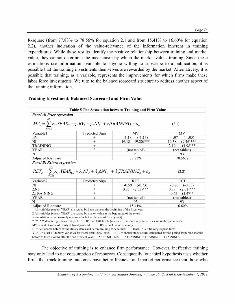
Page 73
Academy of Accounting and Financial Studies Journal, Volume 15, Special Issue Number 1, 2011
R-square (from 77.83% to 78.56% for equation 2.1 and from 15.41% to 16.60% for equation 2.2), another indication of the value-relevance of the information inherent in training expenditures. While these results identify the positive relationship between training and market value, they cannot determine the mechanism by which the market values training. Since these estimations use information available to anyone willing to subscribe to a publication, it is possible that the training investments themselves are rewarded by the market. Alternatively, it is possible that training, as a variable, represents the improvements for which firms make these labor force investments. We turn to the balance scorecard structure to address another aspect of the training information. Training Investment, Balanced Scorecard and Firm Value
Table 5 The Association between Training and Firm Value Panel A: Price regression
∑=
++++=05
023210
YitititittYiYit TRAININGNIBVYEARMV εγγγγ (2.1)
Variable1 Predicted Sign MV MV BV + -1.18 (-1.13) -1.07 (-1.05)NI + 16.18 (9.20)*** 16.38 (9.46)***TRAINING + 2.19 (1.98)**YEAR ? (not tabled) (not tabled)N 93 93 Adjusted R-square 77.83% 78.56% Panel B: Return regression
∑=
++Δ++=05
023210
YitititittYiYit TRAININGNINIYEARRET ελλλλ (2.2)
Variable2 Predicted Sign RET RET NI + -0.59 (-0.73) -0.26 (-0.33)ΔNI + 0.85 (2.38)*** 0.88 (2.51)***ΔTRAINING + 0.63 (1.47)*YEAR ? (not tabled) (not tabled)N 93 93 Adjusted R-square 15.41% 16.60% 1 All variables (except YEAR) are scaled by book value at the beginning of the fiscal year 2 All variables (except YEAR) are scaled by market value at the beginning of the return accumulation period (namely nine months before the end of fiscal year t) *, **, *** denote significance at p= 0.10, 0.05, and 0.01 levels (one-tailed), respectively. t-statistics are in the parentheses. MV = market value of equity at fiscal year end t BV = book value of equity NI = net income before extraordinary items and before training expenditures TRAINING = training expenditures YEAR = a set of dummy variables for fiscal years 2002-2005 RET = annual stock return, calculated for the period from nine months before to three months after the end of fiscal year t ΔNI = NIt-NIt-1 ΔTRAINING = TRAININGt-TRAININGt-1
The objective of training is to enhance firm performance. However, ineffective training may only lead to net consumption of resources. Consequently, our third hypothesis tests whether firms that track training outcomes have better financial and market performance than those who
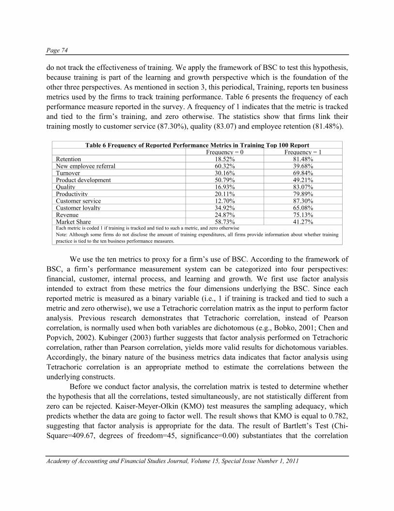
Page 74
Academy of Accounting and Financial Studies Journal, Volume 15, Special Issue Number 1, 2011
do not track the effectiveness of training. We apply the framework of BSC to test this hypothesis, because training is part of the learning and growth perspective which is the foundation of the other three perspectives. As mentioned in section 3, this periodical, Training, reports ten business metrics used by the firms to track training performance. Table 6 presents the frequency of each performance measure reported in the survey. A frequency of 1 indicates that the metric is tracked and tied to the firm’s training, and zero otherwise. The statistics show that firms link their training mostly to customer service (87.30%), quality (83.07) and employee retention (81.48%).
Table 6 Frequency of Reported Performance Metrics in Training Top 100 Report Frequency = 0 Frequency = 1Retention 18.52% 81.48% New employee referral 60.32% 39.68% Turnover 30.16% 69.84% Product development 50.79% 49.21% Quality 16.93% 83.07% Productivity 20.11% 79.89% Customer service 12.70% 87.30% Customer loyalty 34.92% 65.08% Revenue 24.87% 75.13% Market Share 58.73% 41.27% Each metric is coded 1 if training is tracked and tied to such a metric, and zero otherwise Note: Although some firms do not disclose the amount of training expenditures, all firms provide information about whether training practice is tied to the ten business performance measures.
We use the ten metrics to proxy for a firm’s use of BSC. According to the framework of BSC, a firm’s performance measurement system can be categorized into four perspectives: financial, customer, internal process, and learning and growth. We first use factor analysis intended to extract from these metrics the four dimensions underlying the BSC. Since each reported metric is measured as a binary variable (i.e., 1 if training is tracked and tied to such a metric and zero otherwise), we use a Tetrachoric correlation matrix as the input to perform factor analysis. Previous research demonstrates that Tetrachoric correlation, instead of Pearson correlation, is normally used when both variables are dichotomous (e.g., Bobko, 2001; Chen and Popvich, 2002). Kubinger (2003) further suggests that factor analysis performed on Tetrachoric correlation, rather than Pearson correlation, yields more valid results for dichotomous variables. Accordingly, the binary nature of the business metrics data indicates that factor analysis using Tetrachoric correlation is an appropriate method to estimate the correlations between the underlying constructs. Before we conduct factor analysis, the correlation matrix is tested to determine whether the hypothesis that all the correlations, tested simultaneously, are not statistically different from zero can be rejected. Kaiser-Meyer-Olkin (KMO) test measures the sampling adequacy, which predicts whether the data are going to factor well. The result shows that KMO is equal to 0.782, suggesting that factor analysis is appropriate for the data. The result of Bartlett’s Test (Chi-Square=409.67, degrees of freedom=45, significance=0.00) substantiates that the correlation
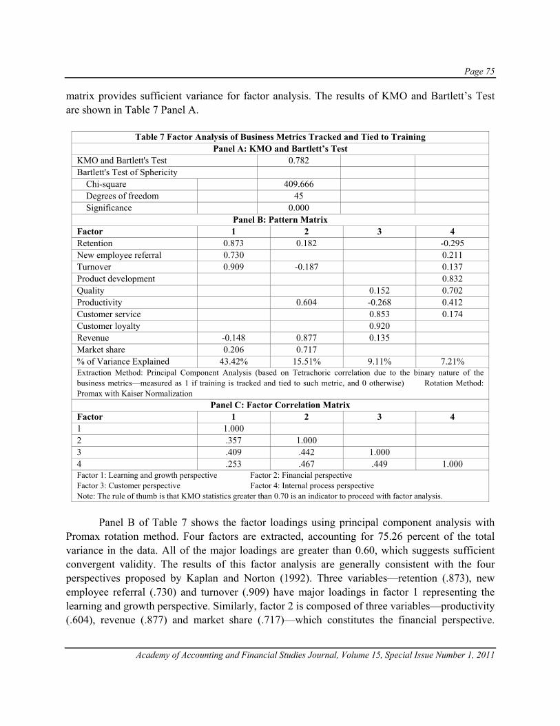
Page 75
Academy of Accounting and Financial Studies Journal, Volume 15, Special Issue Number 1, 2011
matrix provides sufficient variance for factor analysis. The results of KMO and Bartlett’s Test are shown in Table 7 Panel A.
Table 7 Factor Analysis of Business Metrics Tracked and Tied to Training Panel A: KMO and Bartlett’s Test
KMO and Bartlett's Test 0.782 Bartlett's Test of Sphericity Chi-square 409.666 Degrees of freedom 45 Significance 0.000
Panel B: Pattern Matrix Factor 1 2 3 4 Retention 0.873 0.182 -0.295 New employee referral 0.730 0.211 Turnover 0.909 -0.187 0.137 Product development 0.832 Quality 0.152 0.702 Productivity 0.604 -0.268 0.412 Customer service 0.853 0.174 Customer loyalty 0.920 Revenue -0.148 0.877 0.135 Market share 0.206 0.717 % of Variance Explained 43.42% 15.51% 9.11% 7.21% Extraction Method: Principal Component Analysis (based on Tetrachoric correlation due to the binary nature of the business metrics—measured as 1 if training is tracked and tied to such metric, and 0 otherwise) Rotation Method: Promax with Kaiser Normalization
Panel C: Factor Correlation Matrix Factor 1 2 3 4 1 1.000 2 .357 1.000 3 .409 .442 1.000 4 .253 .467 .449 1.000 Factor 1: Learning and growth perspective Factor 2: Financial perspective Factor 3: Customer perspective Factor 4: Internal process perspective Note: The rule of thumb is that KMO statistics greater than 0.70 is an indicator to proceed with factor analysis.
Panel B of Table 7 shows the factor loadings using principal component analysis with Promax rotation method. Four factors are extracted, accounting for 75.26 percent of the total variance in the data. All of the major loadings are greater than 0.60, which suggests sufficient convergent validity. The results of this factor analysis are generally consistent with the four perspectives proposed by Kaplan and Norton (1992). Three variables—retention (.873), new employee referral (.730) and turnover (.909) have major loadings in factor 1 representing the learning and growth perspective. Similarly, factor 2 is composed of three variables—productivity (.604), revenue (.877) and market share (.717)—which constitutes the financial perspective.

Page 76
Academy of Accounting and Financial Studies Journal, Volume 15, Special Issue Number 1, 2011
Customer service (.853) and customer loyalty (.920) are loaded in factor 3, which indicates the customer perspective. The remaining two variables, product development (.832) and quality (.702), represent factor 4—the internal process perspective. The factor correlation matrix in Panel C of Table 7 demonstrates discriminant validity of the factors: The correlations vary from .253 (between factor 1 and factor 4) to .467 (between factor 2 and factor 4), indicating adequate conceptual separation among the factors. After extracting the four factors, we calculate factor scores for each perspective by multiplying the factor loadings by the metrics underlying each factor, and use the factor scores to measure the firm’s use of BSC in conjunction with training. Our third hypothesis argues that linking training to nonfinancial performance measures has an indirect effect on firms’ market values through a direct effect on financial performance measures, therefore we use the two-stage least squares (2SLS) approach to estimate the following models:
05
0 1 2 3 402
it t t it it it it itt
FIN YEAR CUST IP LEARN SIZEδ δ δ δ δ ε=
= + + + + +∑ (3.1)
ititititit
t
tttit ROALEVSIZEFINYEARMV εθθθθθ +++++= ∑
=
=4321
05
020 (3.2)
where FIN is the factor score of the financial perspective, CUST is the factor score of the customer perspective, IP is the factor score of the internal process perspective, and LEARN is the factor score of the learning and growth perspective. Since prior literature finds that larger firms are more likely to use a BSC approach to management (Hoque and James, 2000), we include SIZE as a control variable, measured by the natural logarithm of total assets. Equation (3.1) tests the relationship between the use of non-financial performance metrics in the customer, internal process and learning and growth perspectives and the use of financial metrics in the financial perspective. The predicted value of FIN is then used to estimate equation (3.2) which examines the association between the financial perspective and market value. We take the natural logarithm of market value (MV) to transform the variable to a normal distribution. We also control for size, leverage (measured by debt-to-equity ratio, LEV) and profitability (measured by return on assets, ROA) as determinants of market values. According to Kaplan and Norton (1992, 1993, 2001), the ultimate goal of BSC is to increase shareholder value. Specifically, improvement in the three non-financial perspectives should have a positive effect on the financial perspective, which in turn should increase firm value. Therefore, we predict that δ1>0, δ2>0, δ3>0, and θ1>0. Table 8 provides the results of equations (3.1) and (3.2). According to the estimation of (3.1) in Table 8, the coefficients of CUST, IP and LEARN are all positive and statistically significant. These results suggest that increasing performance tracking of training in each of the non-financial perspectives has positive effect on the use of performance tracking in the financial perspective. The estimation of (3.2) presented in Table 8 shows that the coefficient on FIN is significantly positive, indicating that an improvement in the financial dimension of BSC tied to training has positive effect on the firm’s market value. This is

Page 77
Academy of Accounting and Financial Studies Journal, Volume 15, Special Issue Number 1, 2011
evidence of an indirect relation between non-financial perspectives of BSC and firm value, through its direct effect on financial perspectives. To sum up, when training is used in conjunction with BSC, the use of performance metrics in customer, internal process and learning and growth perspectives is positively related to the use of performance metrics in the financial perspective, which in turn has a positive association with the firm’s market value.
Table 8 The Association between Balanced Scorecard and Firm Value (2SLS) 05
0 1 2 3 402
it t t it it it it itt
FIN YEAR CUST IP LEARN SIZEδ δ δ δ δ ε=
= + + + + +∑ (3.1)
ititititit
t
tttit ROALEVSIZEFINYEARMV εθθθθθ +++++= ∑
=
=4321
05
020 (3.2)
Variable Predicted Sign FIN (3.1) MV (3.2)
CUST + 0.25 (3.26)***
IP + 0.38 (4.33)***
LEARN + 0.20 (3.42)***
FIN + 0.19 (1.58)*
SIZE + 0.01 (0.25)
0.94 (34.70)***
LEV - -0.11 (-11.19)***
ROA + 8.76 (12.64)***
YEAR ? (not tabled) (not tabled) N1 189 189 Adjusted R-square 86.93% 99.66% 1 A total of 400 firm-years in the Training report less 208 non-public observations and 3 observations with missing values in Compustat *, **, *** denote significance at p= 0.10, 0.05, and 0.01 levels, respectively (one-tailed). t-statistics are in the parentheses. FIN = factor score of the financial perspective CUST = factor score of the customer perspective IP = factor score of the internal process perspective LEARN = factor score of the learning and growth perspective MV = natural logarithm of market value of equity at fiscal year end SIZE = natural logarithm of total assets LEV = total debt divided by total equity ROA = net income before extraordinary items divided by average total assets YEAR = a set of dummy variables for fiscal years 2002-2005

Page 78
Academy of Accounting and Financial Studies Journal, Volume 15, Special Issue Number 1, 2011
ROBUSTNESS TESTS
The Influence of Outliers In order to test whether the previous results are sensitive to the influence of outliers, we remove influential observations identified on the basis of criteria developed by Belsley et al. (1980). More specifically, an observation is defined as an outlier if it meets the following criteria: absolute value of DFFITS > 2(p/n)0.5 (p is number of parameters and n is number of observations) or absolute value of studentized residual > 3. The results indicate that all of the above analyses do not change after removal of these outliers. Deflator Effect We test the robustness of our empirical results on equations (1.1) and (1.2) to different deflators of variables. Instead of scaling all variables by number of employees, we use lagged sales and lagged assets as alternative deflators. The results are similar to the ones provided in Table 4, supporting our hypotheses that investment in employee training is positively related to both contemporaneous and future operating performance. Alternative Model Specifications Recognizing that levels specification is more susceptible to omitted variable problem, we conduct a change analysis on equation (1.1), where all variables (except the YEAR indicator) are measured as the change from year t-1 to year t. Untabulated results show that training has significantly positive relationship with operating income. Market Incorporation of Information Since the Training Top 100 report is published in March, we are aware that investors may not incorporate this information from the other financial reports in setting the market price at fiscal year-end. Allowing the market to adjust to the release of new information, we estimate the valuation model (equation 2.1) using the market values of three and six months after fiscal year-end; the results are not sensitive to this specification. In addition, a similar test is performed for equation (3.2) where the log of market value is used, and we obtain similar findings. Further, the market may place a higher valuation on firms that recur in the training report during the sample years than on firms that appear only once. The data show that, among the 46 sample firms, 24 firms are included in the report for two or more years while 22 firms are included in only one year. Therefore, we include a dummy variable that controls for firm

Page 79
Academy of Accounting and Financial Studies Journal, Volume 15, Special Issue Number 1, 2011
recurrence (1 if firms appear in the sample only once and 0 otherwise); the results are robust to this control. Self-Selection Bias Although we do not find significantly different characteristics between firms disclosing a training amount and those not disclosing, it is possible that unobserved variables lead to a self-selection problem. Therefore, we use the Heckman (1979) procedure to address this issue. For H1.1 (the contemporaneous effect of training on operating performance), we estimate the following two-equation model:
itititititit REGREVEMPROESIZEDIS εωωωωω +++++= 43210 (4.1)
∑=
− +++++=05
02431210
YititititittiYYit IMRTAPERFTRAININGYEARPERF εααααα (4.2)
where DIS is a dichotomous variable that equals 1 for firms that disclose training amount, and 0 otherwise. Equation (4.1) uses a Logit regression to estimate the probability of a firm’s disclosing a training amount to the public. The explanatory variables in equation (4.1) are identified in reference to Ballester et al. (2002), which finds that voluntary disclosers of labor-related costs are larger (measured by SIZE, natural logarithm of total assets), more profitable (measured by ROE, return on equity), more labor-intensive (measured by REMEMP, revenues per employee, Lower values of revenues per employee indicate higher labor-intensity), and are operating in regulated industries (measured by REG, a dummy variable which equals one for firms with two-digit SIC codes 40, 46, 48, 49, and 60-64, and zero otherwise). We then derive the inverse Mill’s ratio from the output of equation (4.1) and include this ratio (denoted IMR) in equation (4.2), which uses OLS regression to model the relationship between training and operating performance. All the variables in equation (4.2), except IMR, are the same as those in equation (1.1). We employ the same procedure for H1.2 (the future effect of training on operating performance) and H2 (the effect of training on market valuation/stock returns). The results of the two-equation model are presented in Table 9. Panel A of Table 9 shows the results of the first-stage logit model. All independent variables are not significant; this is consistent with the t-test results described in section 3.1, namely, firms disclosing training amount do not differ significantly from the non-disclosing firms. Panel B reports the second-stage OLS regression results after controlling for self-selection. The results show that training is positively related to both contemporaneous and future operating performance, consistent with the main findings. Further, the magnitude of the coefficient on training is similar to that presented in Table 4. In general, the coefficient of IMR (the inverse Mill’s ratio) is not significant, suggesting that self-selection does not appear to be a significant factor that drives the results. The untabluated results on the second-stage Heckman model for H2

Page 80
Academy of Accounting and Financial Studies Journal, Volume 15, Special Issue Number 1, 2011
also indicate a positive and significant relationship between training and market valuation/stock returns, supporting our primary findings presented in Table 5.
Table 9 The Association between Training, Operating Performance, and Market Value after Controlling for Self-Selection using the Heckman Model
Panel A: Disclosure Logit Model (first-stage)
itititititit REGREVEMPROESIZEDIS εωωωωω +++++= 43210 Variable Predicted Sign Coefficient Std. Error Chi-square Intercept ? -0.25 0.60 0.17 SIZE + 0.02 0.07 0.09 ROE + -0.78 0.66 1.40 REVEMP - 0.0002 0.0003 0.40 REG + 0.30 0.26 1.33 N1 174 Panel B: Relationship between Training and Operating Performance (second-stage) Variable2 Predicted Sign PERFt PERFt+1 PERFt+2
TRAININGt + 2.55 (1.39)*
5.34 (2.32)**
6.88 (2.94)***
PERFt-1 + 0.86 (12.37)***
PERFt + 0.76 (9.36)***
0.86 (10.38)***
TAt ? 0.01 (3.82)***
0.01 (3.29)***
0.01 (3.85)***
IMRt ? 20.52 (0.72)
-43.92 (-1.26)
-67.29 (-1.89)*
YEAR ? (not tabled) (not tabled) (not tabled) N 88 88 88 Adjusted R-square 93.89% 93.27% 94.79% 1 After excluding all missing values in financial variables from Compustat 2 All variables (except YEAR) are scaled by number of employees of year t *, **, *** denote significance at p= 0.10, 0.05, and 0.01 levels (one-tailed), respectively. t-statistics are in the parentheses. DIS = 1 if the firm discloses training amount in the survey report, and 0 otherwise SIZE = total assets natural logarithm of total assets ROE = return on equity REG = 1 if the firm operates in industries with two-digit SIC code 40, 46, 48, 49, or 60-64, and 0 otherwise PERF = operating income after depreciation TRAINING = training expenditures TA = total assets IMR = inverse Mill’s ratio YEAR = a set of dummy variables for fiscal years 2002-2005
Page 81
Academy of Accounting and Financial Studies Journal, Volume 15, Special Issue Number 1, 2011
SUMMARY AND CONCLUSIONS In today’s economy, it has been widely agreed that intangible assets are often far more important to a company’s success than tangible assets. Intellectual human capital, in particular knowledge and competence of employees, is one of the most important sources of companies’ competitive advantages. However, while the existence of physical and financial assets is recognized in the financial statements, U.S. accounting standards require expensing of all internally-generated intangibles. Various studies have shown that investments in intangibles such as R&D and advertising contribute significantly to firms’ profitability and market values (see Lev, 2001). On the other hand, the empirical determination of whether human capital investment such as employee training generates economic benefits and increases firm value is seriously hampered by the lack of publicly disclosed information on such practices, despite frequent assertions to the effect that “employees are our most valuable asset” in companies’ annual reports. This paper uses a unique data source regarding employee training practices to empirically examine the market implication of such human capital investment. Using the 2003-2006 Training Top 100 survey reports published by Training magazine, we first test the relationship between employee training expenditures and firms’ operating performance and market values. For a sample of public companies, we find that training expenditures are significantly and positively related to both contemporaneous and future operating performance. The results suggest that investment in employee training creates economic benefits beyond the current period and lasts for at least two years. In addition, training expenditures are positively related to market values and have significant incremental power in explaining stock returns, suggesting that capital market participants consider this information value-relevant. In addition to the dollar amount of training expenditures, we further use the qualitative information provided in the survey to investigate the market implication of the joint use of training with various performance measures. According to scholars in the field of strategic human resources management, human resources practices produce more benefits when used in alignment with the firm’s strategy and performance measurement system. The balanced scorecard framework proposed by Kaplan and Norton (1992) also advocates the use of both non-financial and financial measures to translate organizational strategy into action which in turn creates shareholder value. From the business metrics reported in the survey, we use factor analysis and extract four principal components consistent with the four perspectives underlying the BSC framework—financial perspective, customer perspective, internal process perspective and learning and growth perspective. We test and find that training in conjunction with the use of metrics in the three non-financial perspectives has a positive relationship with that in the financial perspective, which in turn is positively associated with firms’ market values. These results support the BSC’s theoretical argument that an improvement of non-financial
Page 82
Academy of Accounting and Financial Studies Journal, Volume 15, Special Issue Number 1, 2011
performance measures has an indirect effect on firm value, through a direct effect on the improvement of financial performance measures. Similar to most research in the field of human capital, we have a small sample size due to limited information disclosures and data accessibility. A review by Tharenou et al. (2007) shows that studies on employee training contain observations ranging from 20 to 2079. A closer examination reveals that 20 out of the 67 studies discussed in their paper have sample size of less than 100 observations. Since the financial statements do not provide detailed information about human capital investment (for instance, Compustat provides an aggregate number on labor-related expense but does not differentiate employee training from other expenses), survey is regarded to be one of the acceptable ways of data collection. As far as the limitation of survey data is concerned, this problem is likely to persist in the near future. Due to the nature of specialized data used in this study, the generalizability of our findings is limited. The primary objective of this paper is to explore the quantitative and qualitative attributes of training using the constrained data set available, in an attempt to shed light on this important but poorly-investigated field. This position is consistent with the findings of Tharenou et al. (2007), suggesting that research on training shares limitations in sample size and data accessibility; such limitations may be addressed in future research if more data become available. Nevertheless, the data limitations do not diminish the importance of the research questions and the significance of the findings. This study contributes to both the intangibles literature in accounting and the human capital literature in management by integrating the empirical methodology to examine the capital market effect of an important investment in intangibles. Further, we provide empirical evidence of a linkage between internal non-financial performance and external financial performance which affects market values. Our findings not only have implications for companies’ human resources practices and the associated performance measurement, but also shed light on the impact of BSC implementation on external reporting. Theory predicts that the benefits of BSC, a driver of long-term performance, should be reflected in a firm’s share price. In addressing the question regarding the information value of BSC implementation to the investment community, Kaplan and Norton (1993) cites the limitations of financial reporting standards as the primary reason that explains their failure to find a trend of market reaction to the adoption of BSC. Nevertheless, our paper provides evidence of a significantly positive association between shareholder value and the use of balanced scorecard in connection to training, suggesting a shift in the market perception over the past decade. Given this finding, future research to revisit the topic of balanced scorecard implementation and external reporting could be fruitful. The results of this study also provide insight upon the controversial questions as to the treatment of human capital expenditures. Our findings suggest the training costs, required to be expensed under current U.S. accounting standards, contain characteristics of an asset-like investment in improving firm performance and market valuation.

Page 83
Academy of Accounting and Financial Studies Journal, Volume 15, Special Issue Number 1, 2011
REFERENCES American Accounting Association (1973). Report of the Committee on Human Resource Accounting. The
Accounting Review, 48 (supplement), 169-185. American Accounting Association (1974). Report of the Committee on Accounting for Human Resources. The
Accounting Review, 49 (supplement), 115-124. Aboody, D. & B. Lev (1998). The Value Relevance or Intangibles: The Case of Software Capitalization. Journal of
Accounting Research, 36 (supplement), 161-191. Amir, E. & G. Livne (2005). Accounting, Valuation and Duration of Football Player Contracts. Journal of Business
Finance and Accounting, 32 (3&4), 549-586. Ballester, M., J. Livnat & N. Sinha (2002). Labor Costs and Investments in Human Capital. Journal of Accounting,
Auditing and Finance, 17 (4), 351-373. Ballot G., F. Fakhfakh, & E. Taymaz (2006). Who Benefits from Training and R&D, the Firm or the Workers.
British Journal of Industrial Relations, 44 (3), 473-495. Barth, M. E. & G. Clinch (1998). Revalued Financial, Tangible, and Intangible Assets: Associations with Share
Prices and Non-Market-Based Value Estimates. Journal of Accounting Research, 36 (supplement), 199-217.
Barth, M. E. et al. (1998). Brand Values and Capital Market Valuation. Review of Accounting Studies, 3(1&2), 41-
68. Bartel, A. P. (1994). Productivity Gains form the Implementation of Employee Training Programs. Industrial
Relations, 33 (4), 411-425. Bartel, A. P. (2000). Measuring the Employer’s Return on Investments in Training: Evidence from the Literature.
Industrial Relations, 39 (3), 502-524. Becker, G. S. (1962). Human Capital: A Theoretical Analysis. Journal of Political Economy, 70 (5), 9-49. Becker, G. S. (1964). Human Capital: A Theoretical and Empirical Analysis with Special Reference to Education.
New York, NY: Columbia University Press. Belsley, D., E. Kuh, &R. Welsch (1980). Regression Diagnostics: Identifying Influential Data and Sources of
Collinearity. New York, NY: Wiley. Black, S. E. & L. M. Lynch (1996). Human Capital Investments and Productivity. American Economic Review, 86
(2), 263-267. Blundell, R. et al. (1999). Human Capital Investment: The Returns from Education and Training to the Individual,
the Firm and the Economy. Fiscal Studies, 20 (1), 1-23.

Page 84
Academy of Accounting and Financial Studies Journal, Volume 15, Special Issue Number 1, 2011
Bobko, P. (2001). Correlation and Regression (2nd edition). Thousand Oaks, CA: Sage Publications. Bontis, N. & J. Fitz-enz (2002). Intellectual Capital ROI: A Causal Map of Human Capital Antecedents and
Consequents. Journal of Intellectual Capital, 3 (3), 223-247. Bouillon, M. L., B. M. Doran & P.F. Orazem (1995). Human Capital Investment Effects on Firm Returns. Journal of
Applied Business Research, 12, (1), 30-41. Brooking, A. (1996). Intellectual Capital: Core Asset for the Third Millennium Enterprise. New York, NY:
International Thomson Business Press. Brummet, R. L., E.G. Flamholtz & W.C. Pyle (1968). Human Resource Measurement: A Challenge for
Accountants. The Accounting Review, 43 (2), 217-224. Cascio, W. F. (1991). Costing Human Resources: The Financial Impact of Behavior in Organizations (3rd edition).
Boston, MA: PWS-Kent. Chen, M., S. Cheng & Y. Hwang (2005). An Empirical Investigation of the Relationship between Intellectual
Capital and Firms’ Market Value and Financial Performance. Journal of Intellectual Capital, 6 (2), 159-176.
Chen, P. Y. & P.M. Popovich (2002). Correlation: Parametric and Nonparametric Measures. Thousand Oaks, CA:
Sage Publications. Chuang, Y. C. (2000). Human Capital, Exports, and Economic Growth: A Causality Analysis for Taiwan. Review of
International Economics, 8 (4), 712-720. Cohen, S., D. Thiraios & M. Kandilorou (2006). Do Non-Financial and Financial Performance Parameters
Interrelate in Practice? Working Paper, Athens University of Economics and Business. Corvers, F. (1997). The Impact of Human Capital on Labor Productivity in Manufacturing Sectors of the European
Union. Applied Economics, 29 (8), 975-987. Delantey, J. & M. Huselid (1996). The Impact of Human Resource Management Practices on Perceptions of
Organizational Performance. Academy of Management Journal, 39 (4), 949-969. Douthat, J. (1970). Accounting for Personnel Training and Development Costs. Training and Development Journal,
24 (6), 2-6. Drucker, P. F. (1999). Knowledge-worker Productivity: The Biggest Challenge. California Management Review, 41
(2), 79-81. Edvinsson, L. & M.S. Malone (1997). Intellectual Capital: Realizing Your Company’s True Value by Finding Its
Hidden Roots. New York, NY: Harper Business. Elias, N. (1972). The Effects of Human Asset Statements on the Investment Decision: An Experiment. Journal of
Accounting Research, 10 (supplement), 215-233.

Page 85
Academy of Accounting and Financial Studies Journal, Volume 15, Special Issue Number 1, 2011
Flamholtz, E. G. (1971).A Model for Human Resource Valuation: a Stochastic Process with Service Rewards. The Accounting Review, 46 (2), 253-267.
Flamholtz, E. G. (1974). Human Resource Accounting. Encino, CA: Dickenson Publishing Company. Frantzen, D. (2000). R&D, Human Capital and International Technology Spillovers: A Cross-country Analysis.
Scandinavian Journal of Economics, 102 (1), 57-75. Friedman, A. & B. Lev (1974). A Surrogate Measure for the Firm’s Investment in Human Resources. Journal of
Accounting Research, 12, (2), 235-250. Guest, D. et al. (2000). Effective People Management: Initial Findings of the Future of Work Study. London:
Chartered Institute of Personnel and Development. Heckman, J.J. (1979). Sample Selection Bias as a Specification Error. Econometrica, 47 (1), 153-161. Hendricks, J. A. (1976). The Impact of Human Resource Accounting Information on Stock Investment Decisions:
An Empirical Study. The Accounting Review, 51 (2), 292-305. Hoque, A. & W. James (2000). Linking Balanced Scorecard Measures to Size and Market Factors: Impact on
Organizational Performance. Journal of Management Accounting Research, 12, 1-17. Huselid, M. A. (1995). The Impact of Human Resource Management Practices on Turnover, Productivity, and
Corporate Financial Performance. Academy of Management Journal, 38 (3), 635-672. Huselid, M. A. & B. Becker (1997). The Impact of High Performance Work Systems, Implementation Effectiveness,
and Alignment with Strategy and Shareholder Wealth. Academy of Management Proceedings, 144-148. Kaplan, R. S. & D. P. Norton (1992). The Balanced Scorecard—Measures That Drive Performance. Harvard
Business Review, 70 (1), 71-79. Kaplan, R. S. & D. P. Norton (1993). Putting the Balanced Scorecard to Work. Harvard Business Review, 71(5),
134-147. Kaplan, R. S. & D. P. Norton (1996). The Balanced Scorecard: Translating Strategy into Action. Boston, MA:
Harvard Business School Press. Kaplan, R. S. & D. P. Norton (2001). Commentary: Transforming the Balanced Scorecard from Performance
Measurement to Strategic Management: Part I. Accounting Horizons, 15(1), 87-104. Kothari, S. & J. Zimmerman (1995). Price and Return Models. Journal of Accounting and Economics 20 (2), 155-
192. Kubinger, K. D. (2003). On Artificial Results due to Using Factor Analysis for Dichotomous Variables. Psychology
Science, 45(1), 106-110.

Page 86
Academy of Accounting and Financial Studies Journal, Volume 15, Special Issue Number 1, 2011
Lajili, K. & D. Zeghal (2006). Market Performance Impacts of Human Capital Disclosures. Journal of Accounting and Public Policy, 25(2), 171-194.
Lau, A. H. & H. Lau (1978). Some Proposed Approaches for Writing Off Capitalized Human Resource Assets.
Journal of Accounting Research, 16(1), 80-102. Lev, B. (2001). Intangibles: Management, Measurement, and Reporting. Washington, D.C.: Brookings Institution
Press. Lev. B. & A. Schwartz (1971). On the Use of the Economic Concept of Human Capital in Financial Statements. The
Accounting Review, 46 (1), 103-112. Mincer, J. (1958). Investment in Human Capital and Personal Income Distribution. Journal of Political Economy, 66
(4), 281-302. Morse, W. J. (1973). A Note on the Relationship between Human Assets and Human Capital. The Accounting
Review, 48 (3), 589-593. Ohlson, J. (1995). Earnings, Book Values and Dividends in Security Valuation. Contemporary Accounting
Research, 11 (2), 661-687. Pfeffer, J. (1994). Competitive Advantage Through People. Boston, MA: Harvard Business School Press. Psacharopoulos, G. (1973). Returns to Education: An International Comparison. San Francisco, CA: Jossey-Bass. Pulic, A. (2000 a). VAIC—An Accounting Tool for IC Management. available at www.measuring-
ip.at/papers/ham99txt.htm Pulic, A. (2000 b). MVA and VAIC Analysis of Randomly Selected Companies from FTSE 250. available at
www.vaic-on.net/downloads/ftse30.pdf Roos, G. & J. Roos (1997). Measuring Your Company’s Intellectual Performance. Long Range Planning, 30(3),
413-426. Roos, J. et al. (1998). Intellectual Capital: Navigating in the New Business Landscape. New York, NY: New York
University Press. Russell, J. S., J. R. Terborg & M. L. Powers (1985). Organizational Performance and Organizational Level Training
and Support. Personnel Psychology, 38 (4), 849-863. Schuler, R. S. (1992). Strategic Human Resource Management: Linking People with the Needs of the Business.
Organizational Dynamics, 21 (1), 18-32. Schultz, T. W. (1961). Investment in Human Capital. American Economic Review, 51(1), 1-17. Snell, S. A. & J.W. Dean (1992). Integrated Manufacturing and Human Resource Management: A Human Capital
Perspective. Academy of Management Journal, 35 (3), 467-504.

Page 87
Academy of Accounting and Financial Studies Journal, Volume 15, Special Issue Number 1, 2011
Stewart, T. A. (1994). Your Company’s Most Valuable Asset: Intellectual Capital. Fortune, 130 (7), 28-33. Tharenou, P., A. M. Saks & C. Moore (2007). A Review and Critique of Research on Training and Organizational-
level Outcomes. Human Resource Management Review, 17(3), 251-273. Wright, P. M. & G. C. McMahan (1992). Theoretical Perspective for Human Resource Management. Journal of
Management, 18 (2), 294-320. Youndt, M. et al. (1996). Human Resource Management, Manufacturing Strategy and Firma Performance. Academy
of Management Journal, 39 (4), 836-866. Zuker, L. G., M. R. Darby, & M. B. Brewer (1998). Intellectual Human Capital and the Birth of U.S. Biotechnology
Enterprises. American Economic Review, 88 (1), 290-306.

Page 88
Academy of Accounting and Financial Studies Journal, Volume 15, Special Issue Number 1, 2011
Page 89
Academy of Accounting and Financial Studies Journal, Volume 15, Special Issue Number 1, 2011
INTERNATIONAL PORTFOLIO DIVERSIFICATION BASED ON PARTIAL-CORRELATION
Askar Choudhury, Illinois State University
G. N. Naidu, Illinois State University
ABSTRACT Potential for international portfolio diversification and its rewards has been recognized by the investors and researchers alike for a long-time. Portfolio that has the highest level of expected return for a given level of risk is recognized as mean-variance efficient. Thus, the risk-reward ratio of an internationally diversified portfolio is expected to be higher because of added diversification opportunity due to socio-economic distance between countries. Advantage of portfolio diversification transpires from the drive of risk minimization and maximization of the expected return. In this paper, we implement a portfolio selection method based on partial-correlation proposed by Choudhury and Naidu (2009). This approach utilizes market relationship that is unimpeded by world market influence. Portfolios are constructed using both partial-correlation approach and Markowitz (correlation) approach in the ASEAN countries for two different home markets, Japan and Singapore. Performances of these internationally diversified portfolios have been measured for three different strategies to explore the optimum proportion of asset allocation in the portfolio composition. Research results reveal that, the portfolio based on partial-correlation approach is comparable to portfolio created based on Markowitz approach according to Sharpe’s performance measure. In addition, the optimum strategy that minimizes the coefficient of variation to attain the optimal proportion of asset allocation has a better potential for diversification in the international investment perspective.
INTRODUCTION Portfolio diversification benefit emerges from the motivation of minimizing risk and maximizing the return. Investors have expanded their investment into the international arena for diversification purposes. Although, controlling risk in international market is much more challenging because of number factors involved (see, Sullivan, 2008; Lin, 2000; Brennan & Cao, 1997) that are dynamic in nature. The degree of benefits and rewards from international portfolio diversification supersedes all these impediments. An extensive discussion in this area of research can be found in Solnik (1988). A measure of portfolio risk is the variance of a portfolio. However, portfolio variance depends on the variance of each asset and also the correlations among themselves. Researchers (Grubel, 1968; Bailey & Stulz, 1990; Divecha et al, 1992; Michaud et al. 1996) have demonstrated that relatively low correlations between equity markets

Page 90
Academy of Accounting and Financial Studies Journal, Volume 15, Special Issue Number 1, 2011
in the international arena produces optimum portfolio when diversification is sought. Correlation plays an important function in the creation of diversified portfolio for investment purposes. This “Markowitz” approach of portfolio diversification based on correlation was extended to international portfolio diversification (Levy & Sarnat, 1970; and Solnik, 1974) to gain potential benefits. However, the spurious nature of correlation between country indexes due to global market influence may impact the likely benefits of international diversification. Different alternative methodologies have been suggested by researchers to alleviate this deficiency (Choudhury & Naidu, 2009; Statman & Scheid, 2008; Naidu & Choudhury, 2006; Jorion, 1985; Solnik & Roulet, 2000; Das & Uppal, 2004). Choudhury and Naidu (2009) have proposed the concept of partial-correlation with respect to the world market to mitigate this effect of global market influence on diversified portfolio creation in the European Union (EU) countries. This paper, implements this concept of portfolio diversification in the ASEAN (Association of Southeast Asian Nations) stock markets. Bilateral and multilateral trade agreements among nations have been around for several decades. Recently, an upsurge of trade coalitions began with the signing of North American Free Trade Agreement (NAFTA). European nations also started their efforts to create single European Union (EU). Similarly, Asian nations started positioning themselves to form trade associations of their own, such as, Association of Southeast Asian Nations (ASEAN). In a recent study, Francois and Wignaraja (2008) tested international input-output structural model on data for these ASEAN countries including India. The membership of ASEAN nations grew to 10 countries over the last 15 years. The purpose of all these trade alliances is to eliminate the trade barriers among the member nations and thereby achieve economic prosperity and stability in the region and consequently throughout the whole world. As the trade coalition fosters economic prosperity and income growth, capital formation of member nations will expand. This will pave the way to initiate capital market integration and may not be a desirable aspect for investment diversification purpose. However, absolute economic integration among the member countries takes long time to develop and mature. In the meantime investors can find opportunities to diversify their portfolios within the region or outside. Thus, the primary purpose of this paper is to examine the risk-return tradeoffs prevailing in the capital markets of member nations of ASEAN coalition for investment diversification. We also include countries outside the region in our analysis to observe the differences in outcomes due to different compositions of portfolio diversification. This paper, applies partial-correlation structure of market returns proposed by Choudhury and Naidu (2009) to generate alternative set of diversified portfolios. By implementing this concept, we remove the global market influence of the world economy to diminish the world market effect for an equitable diversified portfolio creation. We also examine the correlation structure of market returns of these countries to create diversified portfolios for comparison purposes. We place emphasis on the alternative prospects for insider (within the coalition) and outsider (outside the coalition) countries.

Page 91
Academy of Accounting and Financial Studies Journal, Volume 15, Special Issue Number 1, 2011
We implement optimization procedure on the coefficient of variation (CV) to determine the proportion of asset allocation in ASEAN countries for both Japanese and Singaporean investors. We then evaluate their performance using Sharpe’s Index and compare them with portfolios created by simple correlation criterion. Results based on performance measure indicate that partial-correlation approach (i.e., partialing out the influence of the world market) is comparable to Markowitz approach (correlation based). Another interesting finding is that, home country strategy (HOME) has the poorest performance among the three different strategies explored in this research.
THEORETICAL BACKGROUND AND STATISTICAL METHODS As the global market in the international arena becomes more integrated, developed markets have displayed greater synchronization compared to emerging markets. Therefore, recently energized emerging markets and their increasing involvement into the world market creates an opportunity for portfolio diversification. Collectively all national equity markets together creates global capital market. Then, if we aggregate all the national equity markets we have a great world equity market. Each national equity market has its own degree of volatility. However, the volatility relative to each other will be different. In the same way equity’s volatility relative to an index will be different. Just as one can estimate the risk of an asset relative to a market index, one can also estimate the risk of a national equity market relative to world equity market. Thus, a country’s correlation is the measure of its market’s sensitivity to world market variability. Bekaert and Harvey (1997) concluded that market volatility is a function of the openness of its economy. Therefore, a country’s correlation is indicative of closeness (or remoteness) of their equity markets. Thus, smaller the correlation the more segmented is the country’s market and hence better will be the gains from diversification. This concept of smaller the degree of correlation the greater the benefit of diversification was popularized by Harry Markowitz (1959). The idea of risk reduction using the correlation structure of returns determines the extent of benefits derived through diversification. However, in the context of global market the degree of correlation between two markets is also influenced by aggregated world market. Therefore, the apparent magnitude of a correlation between two specific markets may be due to the influence of world market on those markets. As for example, the level of correlations between France & Japan and France & Singapore has decreased dramatically from 0.242078 and 0.281069 to -0.01293 and 0.135848 (see Table 1) respectively when calculated as partial-correlation with respect to the world market. Thus, partialing out the influence of world market to create portfolios for diversification may lead to a better investment performance. Thus, the difference in correlations and partial-correlations may produce different results in portfolio diversification. Therefore, even though France and Japan or France and Singapore had higher degree of correlations (0.24 & 0.28), their partial-correlations imply that they may

Page 92
Academy of Accounting and Financial Studies Journal, Volume 15, Special Issue Number 1, 2011
offer better gains from diversification compared to other markets that do not have such an overpowering world market influence. In fact, France moved up to the first portfolio level from the fourth portfolio level when portfolios are created by partial-correlations instead of correlations (see Exhibit-A and Exhibit-B) from the perspective of Japanese home market. This example demonstrates that gains from diversification may be improved by using partial-correlations rather than the simple correlations. However, the relational stability between two countries for the diversification purposes may be more desirable when their correlations and partial-correlations remain same (or similar) in the long run. On the basis of this concept we develop two sets of portfolios based on: a) correlations and b) partial-correlations as a criterion to compare the performance of diversified portfolios.
2. Japan Investor
3. Japan Investor
4. Japan Investor
China
Vietnam
USA
India
Malaysia
Philippines
Indonesia
Thailand
Germany
France
England
South Korea
1. Singapore Investor
2. Singapore Investor
3. Singapore Investor
4. Singapore Investor
Philippines
England
Malaysia
South Korea
Japan
Thailand
Vietnam
China
USA
India
Germany
France
1. Japan Investor
Exhibit-A [portfolios created using correlation]
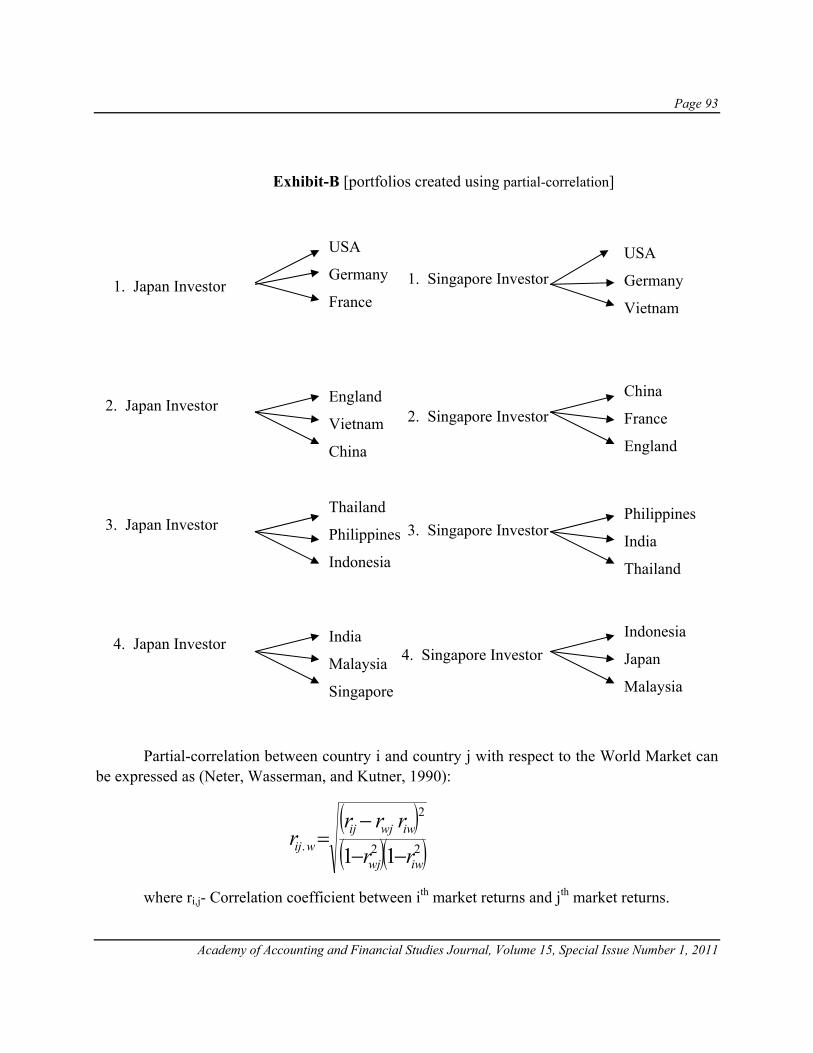
Page 93
Academy of Accounting and Financial Studies Journal, Volume 15, Special Issue Number 1, 2011
Partial-correlation between country i and country j with respect to the World Market can be expressed as (Neter, Wasserman, and Kutner, 1990):
where ri,j- Correlation coefficient between ith market returns and jth market returns.
2. Japan Investor
3. Japan Investor
4. Japan Investor
USA
Germany
France
England
Vietnam
China
Thailand
Philippines
Indonesia
India
Malaysia
Singapore
1. Singapore Investor
2. Singapore Investor
3. Singapore Investor
4. Singapore Investor
Philippines
India
Thailand
Indonesia
Japan
Malaysia
USA
Germany
Vietnam
China
France
England
1. Japan Investor
Exhibit-B [portfolios created using partial-correlation]
( )( )( )22
2
. 11 iwwj
iwwjijwij rr
rrrr
−−
−=
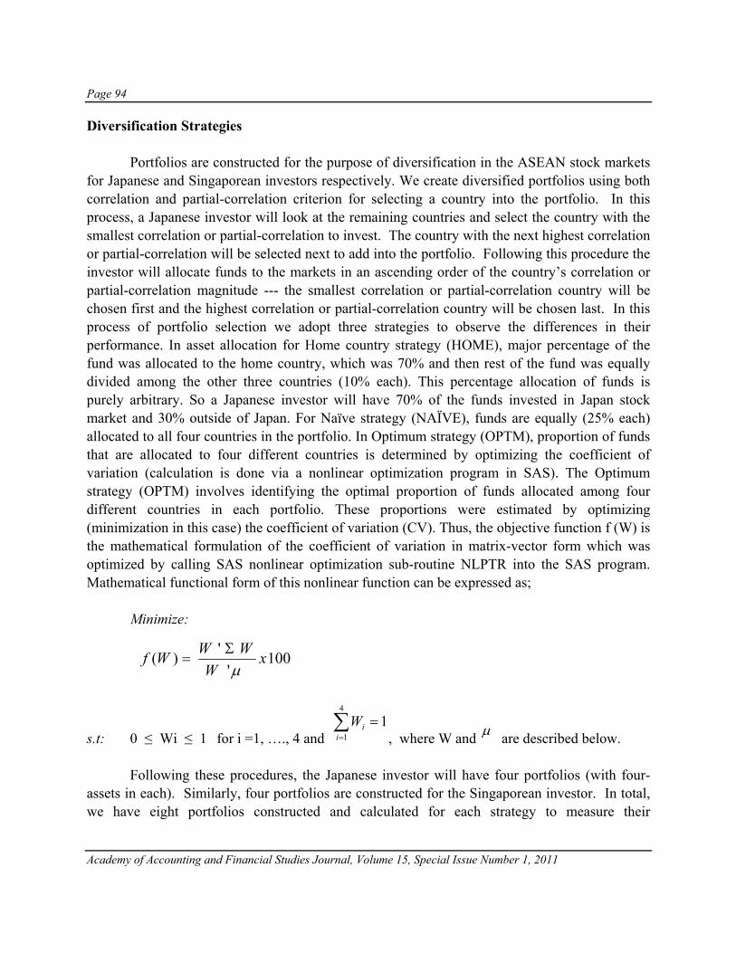
Page 94
Academy of Accounting and Financial Studies Journal, Volume 15, Special Issue Number 1, 2011
Diversification Strategies Portfolios are constructed for the purpose of diversification in the ASEAN stock markets for Japanese and Singaporean investors respectively. We create diversified portfolios using both correlation and partial-correlation criterion for selecting a country into the portfolio. In this process, a Japanese investor will look at the remaining countries and select the country with the smallest correlation or partial-correlation to invest. The country with the next highest correlation or partial-correlation will be selected next to add into the portfolio. Following this procedure the investor will allocate funds to the markets in an ascending order of the country’s correlation or partial-correlation magnitude --- the smallest correlation or partial-correlation country will be chosen first and the highest correlation or partial-correlation country will be chosen last. In this process of portfolio selection we adopt three strategies to observe the differences in their performance. In asset allocation for Home country strategy (HOME), major percentage of the fund was allocated to the home country, which was 70% and then rest of the fund was equally divided among the other three countries (10% each). This percentage allocation of funds is purely arbitrary. So a Japanese investor will have 70% of the funds invested in Japan stock market and 30% outside of Japan. For Naïve strategy (NAÏVE), funds are equally (25% each) allocated to all four countries in the portfolio. In Optimum strategy (OPTM), proportion of funds that are allocated to four different countries is determined by optimizing the coefficient of variation (calculation is done via a nonlinear optimization program in SAS). The Optimum strategy (OPTM) involves identifying the optimal proportion of funds allocated among four different countries in each portfolio. These proportions were estimated by optimizing (minimization in this case) the coefficient of variation (CV). Thus, the objective function f (W) is the mathematical formulation of the coefficient of variation in matrix-vector form which was optimized by calling SAS nonlinear optimization sub-routine NLPTR into the SAS program. Mathematical functional form of this nonlinear function can be expressed as; Minimize:
s.t: 0 ≤ Wi ≤ 1 for i =1, …., 4 and 1
4
1=∑
=iiW
, where W and μ are described below. Following these procedures, the Japanese investor will have four portfolios (with four-assets in each). Similarly, four portfolios are constructed for the Singaporean investor. In total, we have eight portfolios constructed and calculated for each strategy to measure their
100'
')( xW
WWWfμΣ
=

Page 95
Academy of Accounting and Financial Studies Journal, Volume 15, Special Issue Number 1, 2011
performance. We have evaluated each portfolio performance using Sharpe’s Index. The risk-return characteristics of these portfolios are estimated for the thirteen year period, 1995-2007. We hope to demonstrate that partial-correlation based approach to portfolio diversification proposed by Choudhury and Naidu (2009) offers a new way to build internationally diversified portfolios. Performance Measure: Performance of a portfolio is evaluated using both return and risk. A portfolio is said to be mean-variance efficient if it possess the highest level of expected return at a given level of risk. Likewise, it is efficient if it has the lowest level of risk for a given level of expected return. Thus, the desire for international diversification is to optimize the risk-reward ratio, which also reinforces the importance of country selection strategy for an optimum portfolio. Portfolios that are diversified internationally have more potential to lower the risk for the same level of expected return, or to increase the return for the same risk level. As a result, the risk-reward ratio of an internationally diversified portfolio is in advantageous position. Coefficient of variation (CV) measures the relative variability and can be used to measure the standardized risk with respect to the mean. Thus, coefficient of variation can be considered a risk-reward ratio. Coefficient of variation of a portfolio return can be expressed as follows:
.
The smaller the CV the better is the performance of the portfolio. Thus, a portfolio is considered to be more diversified if the CV is smaller in magnitude. Another measure of portfolio performance developed by William Sharpe (1966) is composite (risk-adjusted) in nature and known as the reward-to-variability ratio. This measure is also called Sharpe’s Performance Index (PI) and is expressed as,
.
Where, =pσ standard deviation of pth portfolio return, =pμ average return of pth portfolio, r= risk- free rate for this period. Therefore, the higher the values of the index better the performance of that portfolio on risk-adjusted basis. The Performance of a diversified portfolio will be evaluated by using the expected return and standard deviation of return of a portfolio consisting of proportion of assets invested in the home country and the remaining portion of assets invested in three other countries (or markets).
p
pp
rPI
σμ −
=
100xCVp
pp μ
σ=

Page 96
Academy of Accounting and Financial Studies Journal, Volume 15, Special Issue Number 1, 2011
Thus, we will create and evaluate three different strategies to determine the optimum proportion (weights) of asset allocation in constructing a portfolio. Expected return and variance of a portfolio in matrix-vector form is expressed as follows:
where, W is the vector of portfolio weights (or proportion) for different markets, µ is the mean vector of returns of markets in the portfolio, and Σ is the variance-covariance matrix. For example, the mean and variance of a portfolio with only two markets (assets) can be written as,
Where, =1μ average return of market-1, =2μ average return of market-2, =1σ standard
deviation of return of market-1, =2σ standard deviation of return of market-2, =21σσcovariance of returns between market-1 and market-2.
EMPIRICAL ANALYSIS For our analysis, a set of eight portfolios were created using Markowitz approach (correlation), see the methodology section above. Another set of eight portfolios using partial-correlation as the basis for market (country) selection were also created. These set of portfolios appear in Exhibit-A and Exhibit-B. As can be seen from these exhibits, the least correlated country (asset) portfolios are exactly identical in composition of countries for both Japanese and Singaporean investors. But, the lowest partial-correlation portfolios are not identical in composition of countries. The portfolio composition changes dramatically, however, as the correlation and the partial-correlation levels ascend. For example, the portfolio-2 for Japanese investor has a quite different composition using partial-correlation than correlation criterion. A similar change in composition also occurs to Singaporean investors. Thus, it appears that these two processes of portfolio selection using correlation and partial-correlation as selection basis produces portfolios that are different in composition. Daily data for all the stock market indices of the ASEAN region including some outside countries were obtained from GMID, Global Financial Data, and SourceOECD for the period 1995-2007. The daily returns were computed and annualized. Since, the correlation structure of returns has been one of the bases for diversification (risk reduction) potential. Mean, standard deviation, and correlation structure of annualized daily stock returns among these equity markets have been estimated and presented in Table 1. However, in certain markets the correlation structure may not provide adequate guidance for diversification potential when international diversification is in play. In those circumstances, partial-correlation criteria may offer a greater diversification potential. Thus, in-addition to correlation structure we also estimated partial-
andWp μμ '= WWV p Σ= '
2211 μμμ wwp += 21122122
22
21
21 2 σσσσσ wwwwV p ++=

Page 97
Academy of Accounting and Financial Studies Journal, Volume 15, Special Issue Number 1, 2011
correlation for all these stock markets with respect to the world market. Consequently, partial relationship between two markets that are independent of the world market is observed and reported in Table 1. To represent World Equity Market, we have used Morgan Stanley Capital International Index.
TABLE 1: Means, Standard Deviations, Correlations, and Partial-Correlations of Annualized Daily Stock Market Returns (1995-2007).
Country Japan (Correlations)
Singapore (Correlations)
World (Correlations)
Japan (Partial *
Correlations)
Singapore (Partial *
Correlations) Mean Std Dev
China 0.031433 0.043616 -0.01938 0.106618 0.128181 2.964191 30.63071 India 0.179452 0.249031 0.144674 0.26685 0.349418 2.134652 19.50228
Indonesia 0.209067 0.450305 0.139591 0.262717 0.428728 2.478141 24.25272 Malaysia 0.190205 0.338785 0.111036 0.320849 0.484345 1.731024 25.75152
Philippines 0.194518 0.308432 0.121262 0.246851 0.246366 1.51087 20.79057 South Korea 0.368217 0.367141 0.233157 0.535508 0.506302 3.244774 27.37225
Thailand 0.212969 0.444096 0.175292 0.22863 0.384552 1.662961 22.65673 Vietnam 0.036503 0.008283 -0.03098 0.056254 0.035709 2.893108 21.71856
Singapore 0.37044 1 0.316386 0.468349 1 1.070867 14.68682 Japan 1 0.37044 0.375318 1 0.468349 1.099124 17.24216 USA 0.098289 0.124043 0.861422 -0.45875 -0.41699 1.119374 13.05674
England 0.262567 0.320006 0.680406 0.041697 0.211623 0.849054 11.70755 France 0.242078 0.281069 0.675144 -0.01293 0.135848 1.490869 16.4962
Germany 0.223477 0.271389 0.696651 -0.10227 0.031518 1.682919 17.90263 World 0.375318 0.316386 1 0.740822 9.913175
* Partial-correlations are calculated with respect to World Index.
The mean, standard deviation, coefficient of variation (CV), and Sharpe’s Index for all eight portfolios constructed using the correlation-based (Markowitz) screening criterion is presented in Table 2. All portfolios are evaluated for all three different strategies of proportion of asset allocation. Negative Sharpe’s Index implies that all eight portfolios constructed using Markowitz approach have underperformed the risk-free assets (short-term government debt) in their respective home markets. Degree of performance varied greatly among the portfolios. Nonetheless, optimum diversified portfolio produced higher expected return (e.g., 2.24 and 2.31 for Japanese and Singaporean respectively) for a similar risk level of each portfolio constructed.
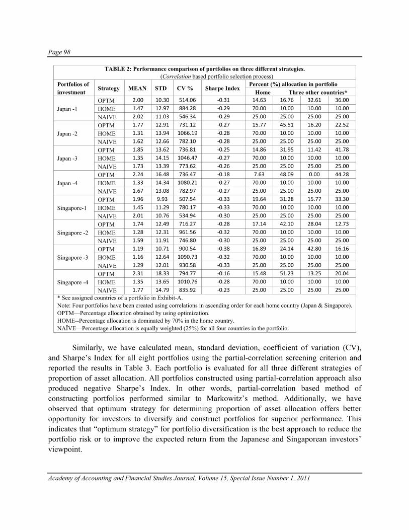
Page 98
Academy of Accounting and Financial Studies Journal, Volume 15, Special Issue Number 1, 2011
TABLE 2: Performance comparison of portfolios on three different strategies. (Correlation based portfolio selection process)
Portfolios of investment
Strategy MEAN STD CV % Sharpe Index Percent (%) allocation in portfolio Home Three other countries*
Japan -1 OPTM 2.00 10.30 514.06 -0.31 14.63 16.76 32.61 36.00
HOME 1.47 12.97 884.28 -0.29 70.00 10.00 10.00 10.00
NAIVE 2.02 11.03 546.34 -0.29 25.00 25.00 25.00 25.00
Japan -2 OPTM 1.77 12.91 731.12 -0.27 15.77 45.51 16.20 22.52
HOME 1.31 13.94 1066.19 -0.28 70.00 10.00 10.00 10.00
NAIVE 1.62 12.66 782.10 -0.28 25.00 25.00 25.00 25.00
Japan -3 OPTM 1.85 13.62 736.81 -0.25 14.86 31.95 11.42 41.78
HOME 1.35 14.15 1046.47 -0.27 70.00 10.00 10.00 10.00
NAIVE 1.73 13.39 773.62 -0.26 25.00 25.00 25.00 25.00
Japan -4 OPTM 2.24 16.48 736.47 -0.18 7.63 48.09 0.00 44.28
HOME 1.33 14.34 1080.21 -0.27 70.00 10.00 10.00 10.00
NAIVE 1.67 13.08 782.97 -0.27 25.00 25.00 25.00 25.00
Singapore-1 OPTM 1.96 9.93 507.54 -0.33 19.64 31.28 15.77 33.30
HOME 1.45 11.29 780.17 -0.33 70.00 10.00 10.00 10.00
NAIVE 2.01 10.76 534.94 -0.30 25.00 25.00 25.00 25.00
Singapore -2 OPTM 1.74 12.49 716.27 -0.28 17.14 42.10 28.04 12.73
HOME 1.28 12.31 961.56 -0.32 70.00 10.00 10.00 10.00
NAIVE 1.59 11.91 746.80 -0.30 25.00 25.00 25.00 25.00
Singapore -3 OPTM 1.19 10.71 900.54 -0.38 16.89 24.14 42.80 16.16
HOME 1.16 12.64 1090.73 -0.32 70.00 10.00 10.00 10.00
NAIVE 1.29 12.01 930.58 -0.33 25.00 25.00 25.00 25.00
Singapore -4 OPTM 2.31 18.33 794.77 -0.16 15.48 51.23 13.25 20.04
HOME 1.35 13.65 1010.76 -0.28 70.00 10.00 10.00 10.00
NAIVE 1.77 14.79 835.92 -0.23 25.00 25.00 25.00 25.00 * See assigned countries of a portfolio in Exhibit-A. Note: Four portfolios have been created using correlations in ascending order for each home country (Japan & Singapore). OPTM—Percentage allocation obtained by using optimization. HOME--Percentage allocation is dominated by 70% in the home country. NAÏVE—Percentage allocation is equally weighted (25%) for all four countries in the portfolio.
Similarly, we have calculated mean, standard deviation, coefficient of variation (CV), and Sharpe’s Index for all eight portfolios using the partial-correlation screening criterion and reported the results in Table 3. Each portfolio is evaluated for all three different strategies of proportion of asset allocation. All portfolios constructed using partial-correlation approach also produced negative Sharpe’s Index. In other words, partial-correlation based method of constructing portfolios performed similar to Markowitz’s method. Additionally, we have observed that optimum strategy for determining proportion of asset allocation offers better opportunity for investors to diversify and construct portfolios for superior performance. This indicates that “optimum strategy” for portfolio diversification is the best approach to reduce the portfolio risk or to improve the expected return from the Japanese and Singaporean investors’ viewpoint.
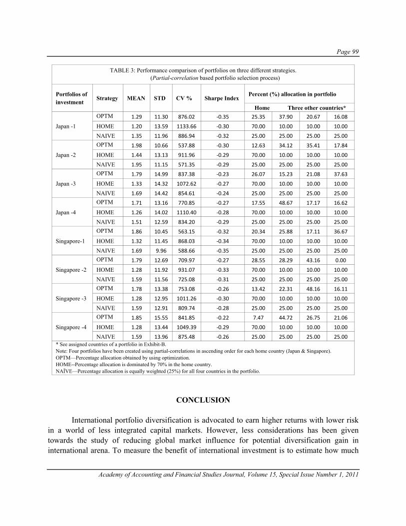
Page 99
Academy of Accounting and Financial Studies Journal, Volume 15, Special Issue Number 1, 2011
TABLE 3: Performance comparison of portfolios on three different strategies. (Partial-correlation based portfolio selection process)
Portfolios of investment
Strategy MEAN STD CV % Sharpe Index Percent (%) allocation in portfolio
Home Three other countries*
Japan -1
OPTM 1.29 11.30 876.02 -0.35 25.35 37.90 20.67 16.08
HOME 1.20 13.59 1133.66 -0.30 70.00 10.00 10.00 10.00
NAIVE 1.35 11.96 886.94 -0.32 25.00 25.00 25.00 25.00
Japan -2
OPTM 1.98 10.66 537.88 -0.30 12.63 34.12 35.41 17.84
HOME 1.44 13.13 911.96 -0.29 70.00 10.00 10.00 10.00
NAIVE 1.95 11.15 571.35 -0.29 25.00 25.00 25.00 25.00
Japan -3
OPTM 1.79 14.99 837.38 -0.23 26.07 15.23 21.08 37.63
HOME 1.33 14.32 1072.62 -0.27 70.00 10.00 10.00 10.00
NAIVE 1.69 14.42 854.61 -0.24 25.00 25.00 25.00 25.00
Japan -4
OPTM 1.71 13.16 770.85 -0.27 17.55 48.67 17.17 16.62
HOME 1.26 14.02 1110.40 -0.28 70.00 10.00 10.00 10.00
NAIVE 1.51 12.59 834.20 -0.29 25.00 25.00 25.00 25.00
Singapore-1
OPTM 1.86 10.45 563.15 -0.32 20.34 25.88 17.11 36.67
HOME 1.32 11.45 868.03 -0.34 70.00 10.00 10.00 10.00
NAIVE 1.69 9.96 588.66 -0.35 25.00 25.00 25.00 25.00
Singapore -2
OPTM 1.79 12.69 709.97 -0.27 28.55 28.29 43.16 0.00
HOME 1.28 11.92 931.07 -0.33 70.00 10.00 10.00 10.00
NAIVE 1.59 11.56 725.08 -0.31 25.00 25.00 25.00 25.00
Singapore -3
OPTM 1.78 13.38 753.08 -0.26 13.42 22.31 48.16 16.11
HOME 1.28 12.95 1011.26 -0.30 70.00 10.00 10.00 10.00
NAIVE 1.59 12.91 809.74 -0.28 25.00 25.00 25.00 25.00
Singapore -4
OPTM 1.85 15.55 841.85 -0.22 7.47 44.72 26.75 21.06
HOME 1.28 13.44 1049.39 -0.29 70.00 10.00 10.00 10.00
NAIVE 1.59 13.96 875.48 -0.26 25.00 25.00 25.00 25.00 * See assigned countries of a portfolio in Exhibit-B. Note: Four portfolios have been created using partial-correlations in ascending order for each home country (Japan & Singapore). OPTM—Percentage allocation obtained by using optimization. HOME--Percentage allocation is dominated by 70% in the home country. NAÏVE—Percentage allocation is equally weighted (25%) for all four countries in the portfolio.
CONCLUSION International portfolio diversification is advocated to earn higher returns with lower risk in a world of less integrated capital markets. However, less considerations has been given towards the study of reducing global market influence for potential diversification gain in international arena. To measure the benefit of international investment is to estimate how much
Page 100
Academy of Accounting and Financial Studies Journal, Volume 15, Special Issue Number 1, 2011
international portfolio diversification with respect to world market can reduce the variance and or increase the expected return of a diversified portfolio compared to the home country’s variance and expected return. In this paper we implement a method of portfolio selection on the basis of partial-correlation criterion proposed by Choudhury and Naidu (2009) by seeking market relationship that is independent of world market. Thus, we have created portfolios using both partial-correlation approach and correlation approach for two different home markets, namely Japan and Singapore. The performance of these portfolios has been measured for three different strategies. Strategies are different in their proportion of asset allocation in the portfolios to identify the optimum portion. As expected, the two different approaches (partial-correlation and correlation) produced portfolios with different composition of markets. Our research analysis also reveals that the optimum strategy that minimizes the coefficient of variation to determine the proportion of asset allocation has a better potential for diversification benefit compared to other strategies. In addition, we have observed that portfolios constructed by partial-correlation approach are very much comparable to Markowitz approach in their performance.
REFERENCES Bailey, W. & R.M. Stulz (1990). Benefits of International Diversification: The Case of Pacific Basin Stock Markets,
Journal of Portfolio Management, 16, 47-61. Bekaert, G. & C. R. Harvey (1997). Emerging Equity Market Volatility. Journal of Financial Economics, 43, 29-77. Bracker, K. & P.D. Koch (1999). Economic Determinants of the Correlation Structure across International Equity
Markets. Journal of Economics and Business, 51, 443-471. Brennan, M.J. & H.N. Cao (1997). International Portfolio Investment Flows. The Journal of Finance, 52(5), 1851-
1880. Chopra, V.K., C.R. Hensel & A.L. Turner (1993). Massaging Mean-Variance Inputs: Returns from Alternative
Global Investment Strategies in the 1980s. Management Science, 39, 845-855. Choudhury, A.H. and G.N. Naidu (2009). A New Selection Strategy for Portfolio Diversification in the European
Union. Academy of Accounting and Financial Studies Journal, Vol. 13(3), 79-92. Das, S.R. and R. Uppal (2004). Systemic Risk and International Portfolio Choice. The Journal of Finance, Vol.
59(6), 2809-2834. DeFusco, R.A., J.M. Geppert & G. Tsetsekos (1996). Long-Run Diversification Potential in Emerging Stock
Markets. Financial Review, 31, 343-363. Divecha, A.B., J. Drach & D. Dtefek (1992). Emerging Markets: A Quantitative Perspective. Journal of Portfolio
Management, 19, 41-50.

Page 101
Academy of Accounting and Financial Studies Journal, Volume 15, Special Issue Number 1, 2011
Errunza, V. R. & P. Padmanabhan (1988). Further evidence on the benefits of portfolio investments in emerging markets. Financial Analysts Journal, 44(4), 76-78.
Francois, J.F. and G. Wignaraja (2008), Economic Implications of Asian Integration, Global Economy Journal, 8(3), 1- 46.
Grubel, H. (1968). International diversified portfolios: Welfare Gains and Capital Flows. American Economic
Review, 5, 1299-1314. Harvey, C. R.. (1991). The world price of covariance risk. Journal of Finance, 46, 111--157. Harvey, C. R.. (1995). Predictable Risk and Returns in Emerging Markets. Review of Financial Studies, 8(3), 773-
816. Jorion, P. (1985). International Portfolio Diversification with Estimation Risk. The Journal of Business, 58(3), 259-
278. Kasa, K. (1992). Common Stochastic Trends in International Stock Markets. Journal of Monetary Economics, 29,
95-124. Lau, S.T. & T.H. McInish (1993). Co-Movements of International Equity Returns: A Comparison of the Pre-and
Post-October 19, 1987, Periods. Global Finance Journal, 4, 1-19. Lessard, D. R. (1974). World, National, and Industry Factors in Equity Returns. Journal of Finance, 29(2), 379-391. Levy, H. & M. Sarnat (1970). International Diversification of Investment Portfolios. American Economic Review,
60, 668–675. Lin, W. (2000). Controlling Risk in Global Multimanager Portfolios. Financial Analysts Journal, 56, 44-53. Markowitz, H. M. (1959). Portfolio Selection. Wiley, New York. Michaud, R.O., G.L. Bergstrom, R.D. Frachure & B. Wolahan (1996). Twenty Years of Equity Financing. Journal
of Portfolio Management, 23, 9-27. Naidu, G.N. & A.H. Choudhury (2006). Country Betas and Potential Gains FromDiversification in the European
Union. Journal of the Academy of Finance, 4(1), 26-36. Neter, J., W. Wasserman & M.H. Kutner, (1990). Applied Linear Statistical Models,3rd ed. Irwin, Homewood,
Illinois. SAS/IML User’s Guide. 1993. SAS Institute, Inc, Cary, North Carolina. Shapiro, A.C. (2003). Multinational Financial Management, 7th Edition, Chichester: John Wiley & Sons. Sharpe, W. (1966). Mutual Fund Performance. Journal of Business, 119-138. Solnik, B.H. (1974). Why do not diversify internationally than domestically? Financial Analyst Journal, 30, 48-54.

Page 102
Academy of Accounting and Financial Studies Journal, Volume 15, Special Issue Number 1, 2011
Solnik, B.H. (1988). International Investment, MA: Addison-Wesley. Solnik, B. & J. Roulet (2000). Dispersion as cross-sectional correlation. Financial Analysts Journal, 56(1), 54-61. Solnik, B. & D. McLeavey (2003). International Investments, 5th ed. Boston:Addison-Wesley. Statman, M. & J. Scheld (2008). Correlation, Return Gaps, and the Benefits of Diversification. The Journal of
Portfolio Management, 34(3), 132-139. Sullivan, R.N. (2008). Taming Global Village Risk. Journal of Portfolio Management, 34(4), 58-67.
Page 103
Academy of Accounting and Financial Studies Journal, Volume 15, Special Issue Number 1, 2011
A CROSS SECTIONAL STUDY OF FINANCIAL MEASURES IN PREDICTING STOCKS’ RISKINESS
DURING YEAR 2008 CRASH PERIOD
Victor Bahhouth, University of North Carolina - Pembroke Ramin Maysami, University of North Carolina - Pembroke
ABSTRACT
The study tests the use of financial measures in predicting stocks’ riskiness during 2008 crash period. The stock market witnessed a number of crashes with the most recent one in year 2008. Crashes cause instability in the stock market and a collapse of investor confidence. In a study, Bahhouth and Maysami (2009) showed evidence that Beta had a marginal effect in predicting stocks riskiness. The paper explores the ability of using financial ratios to identify stocks’ riskiness (i.e. stocks that are more adversely affected during the crash periods). Analysts, practitioners and academicians used financial ratios in assessing stock returns in financial markets (Arslan, O. and Karam, M., 2009; Bhandari 1988; Basu 1977; Tze, S., and Bon H.,2009). The results showed that a set of financial measures exhibited significant predictive power in identifying stocks that were adversely affected during the year 2008 crash period.
INTRODUCTION Several studies discussed the crash of stock markets and suggested different explanations. Roll (1989) suggested downward revised expectations for the worldwide economic activity. Others highlighted that stock prices swing from fundamental values because of the trading activities of the uninformed (Shiller, 1984). Zuckerman E. and Rao H. (2004) related the market crash of year 2000 to the main features of trading in technology stocks early in the 1990s. Investors and stock traders were not able to explain the implications of the rise and fall of the Internet stock for many years. Ofek and Richardson (2003) pointed out that during that period, the very high volume of trade in Internet stocks indicated a wide gap between the prices and their fundamental values. Demers and Lev (2001) gave two broad reasons for how Internet stocks reached unjustifiably high prices in the late 1990s and early 2000. The first focuses on the fundamental values that highlight the elements of capital gains and losses. Investors change their opinion often based on indicators rather than on fundamental values. The second suggests that fundamentals were indeed responsible for market prices but investors’ interpretations of fundamentals were irrationally optimistic in making their assessments. Ang, Tourani-Rad, and Yu (2004) in reporting their findings of 1997 south-east Asia crash period made four major remarks which are the following: 1- Price bubbles exist prior to the
Page 104
Academy of Accounting and Financial Studies Journal, Volume 15, Special Issue Number 1, 2011
crash period. 2- Price momentum increases stock price prior to the crash period. 3- Price bubbles are among the most liquid and most volatile shares. 4- stock liquidity changes during crash periods. In addition, it was noticed that during normal periods, illiquid shares are priced at a discount in comparison with those of more liquid shares. The result is a negative effect on the required rates of return. Contrary to these results, during a crash period, illiquid shares experience a smaller drop in prices. Other researchers (De Long et al., 1993; Shleifer and Vishny, 1997) explained that fundamental limitations on arbitrage might have been responsible. Ofek and Richardson (2003) described a process whereby the significant constraints on the short selling of the Internet stocks prevented the opinions of more reasonable investors from being incorporated into prices. In the early 2000, with the expiration of the lock-up period that prevented insiders from selling stocks, prices of the Internet stocks fell, which led into a price crash (Ofek and Richardson, 2003). Blodget Henry (2005) referred the market crash of year 2000 to the prevailing strategies like "buy and hold" that had been applied for more than a decade. A large number of new market traders believed that 20-percent annual return was normal. In the hindsight, the only pain that approaches the pain of losing money is the pain of not making money when everyone else is. The NASDAQ stock market, for example, did not hit 5,000 because of fraud or idiocy. It was because the majority of investors made investment decisions that they believed reasonable at that time. This paper tests the use of fundamental measures in identifying risky stocks that are more adversely affected during the year 2008 crash period; the following is the research problem:
• Null Hypothesis: Financial measures don’t identify risky stocks during year 2008 crash period. • Alternate Hypothesis: Financial measures do identify risky stocks during year 2008 crash period.
METHODOLOGY AND DATA DESCRIPTION
This study takes a deep look into the predictive ability of financial measures in determining the stocks’ riskiness during crash periods. The data is a secondary type and is taken from Compustat e-data bank. It covers a twelve-month-period ending by October 31, 2008. The data bank includes the information of the 9870 US publicly traded firms. A binary logistic regression model (BLRM) is used to test the research problem. Logistic regression is superior to linear regression when the normality assumption of the independent variables is not met. It is simpler to read and to interpret because its values are between zero and one (Tsun-Siou, Yin-Hua & Rong-Tze, 2003; Arslan, O. and Baha, M., 2010; ). The use of the logistic regression model in this study is to evaluate the predictive power of the independent variables (fundamental measures) in classifying traded stocks into two groups (dependent variable). The dependent variable is a non-metric measure and is used to identify these two-stock groups; stocks that are adversely affected during crash periods (assigned a value = 0), and stocks that are less adversely affected (assigned a value = 1).
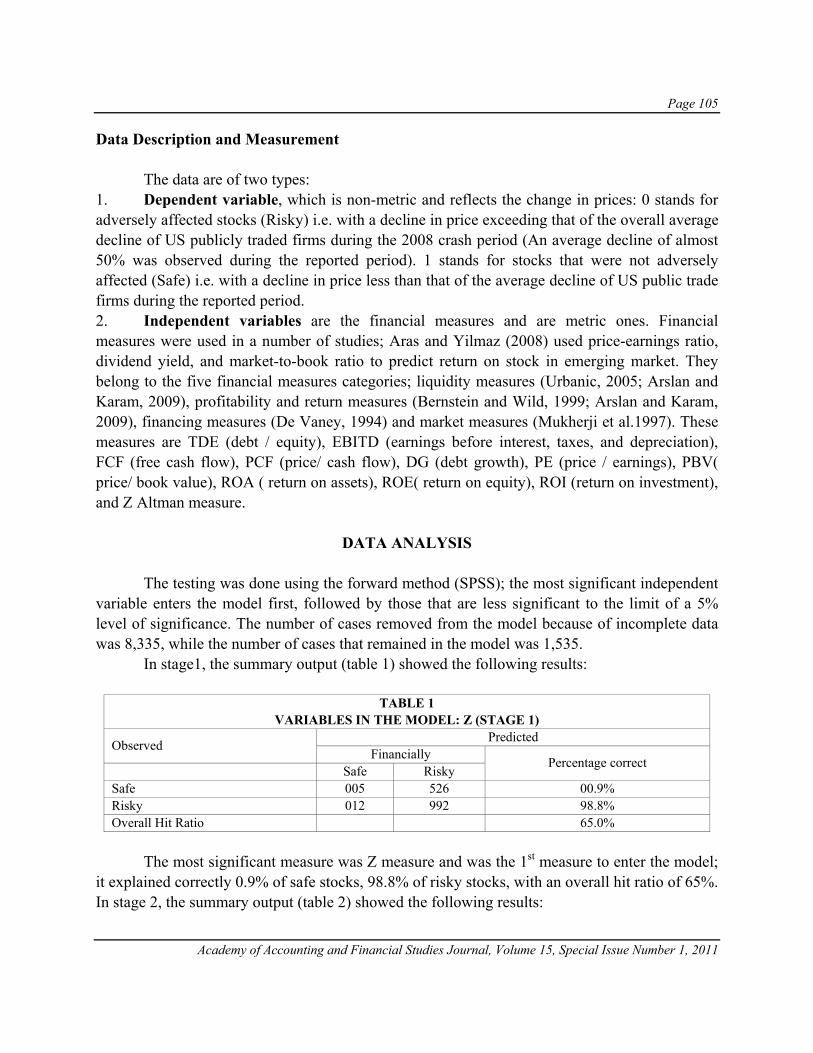
Page 105
Academy of Accounting and Financial Studies Journal, Volume 15, Special Issue Number 1, 2011
Data Description and Measurement The data are of two types: 1. Dependent variable, which is non-metric and reflects the change in prices: 0 stands for adversely affected stocks (Risky) i.e. with a decline in price exceeding that of the overall average decline of US publicly traded firms during the 2008 crash period (An average decline of almost 50% was observed during the reported period). 1 stands for stocks that were not adversely affected (Safe) i.e. with a decline in price less than that of the average decline of US public trade firms during the reported period. 2. Independent variables are the financial measures and are metric ones. Financial measures were used in a number of studies; Aras and Yilmaz (2008) used price-earnings ratio, dividend yield, and market-to-book ratio to predict return on stock in emerging market. They belong to the five financial measures categories; liquidity measures (Urbanic, 2005; Arslan and Karam, 2009), profitability and return measures (Bernstein and Wild, 1999; Arslan and Karam, 2009), financing measures (De Vaney, 1994) and market measures (Mukherji et al.1997). These measures are TDE (debt / equity), EBITD (earnings before interest, taxes, and depreciation), FCF (free cash flow), PCF (price/ cash flow), DG (debt growth), PE (price / earnings), PBV( price/ book value), ROA ( return on assets), ROE( return on equity), ROI (return on investment), and Z Altman measure.
DATA ANALYSIS The testing was done using the forward method (SPSS); the most significant independent variable enters the model first, followed by those that are less significant to the limit of a 5% level of significance. The number of cases removed from the model because of incomplete data was 8,335, while the number of cases that remained in the model was 1,535. In stage1, the summary output (table 1) showed the following results:
TABLE 1 VARIABLES IN THE MODEL: Z (STAGE 1)
Observed Predicted Financially Percentage correct Safe Risky
Safe 005 526 00.9% Risky 012 992 98.8% Overall Hit Ratio 65.0%
The most significant measure was Z measure and was the 1st measure to enter the model; it explained correctly 0.9% of safe stocks, 98.8% of risky stocks, with an overall hit ratio of 65%. In stage 2, the summary output (table 2) showed the following results:
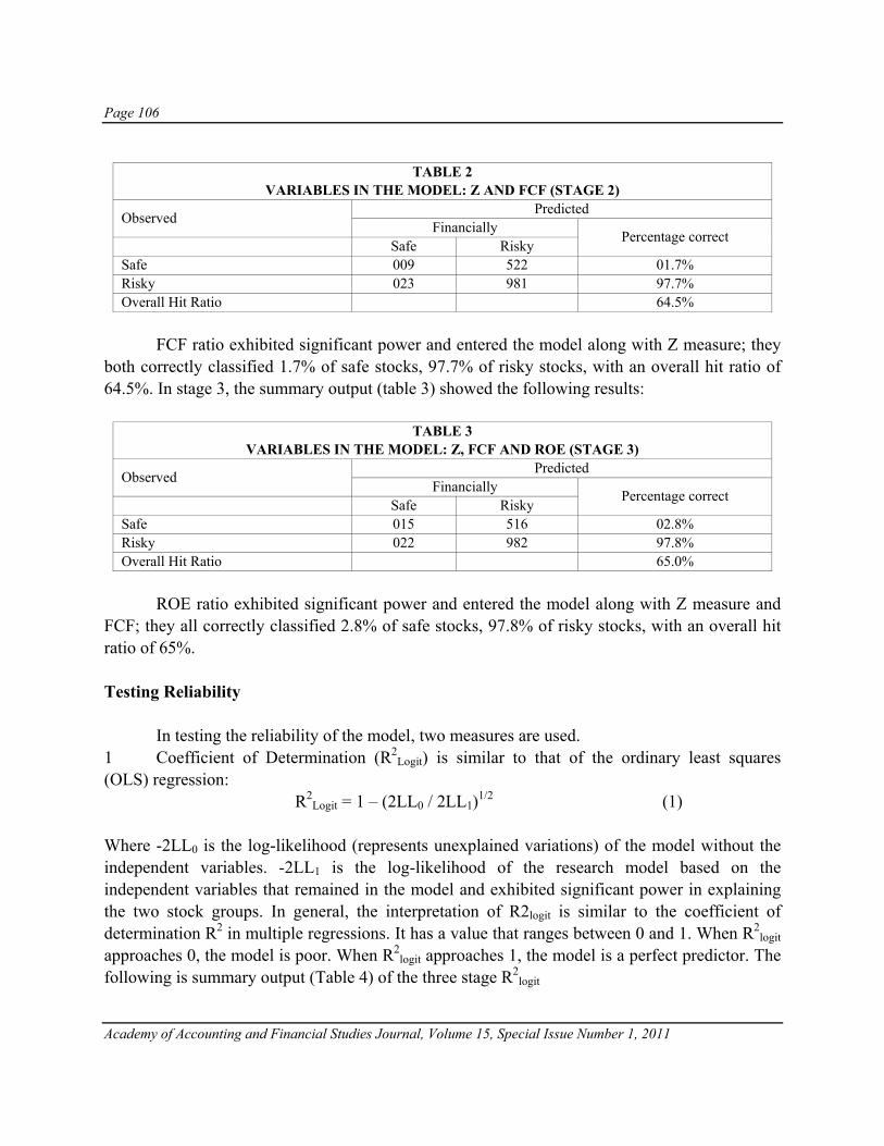
Page 106
Academy of Accounting and Financial Studies Journal, Volume 15, Special Issue Number 1, 2011
TABLE 2
VARIABLES IN THE MODEL: Z AND FCF (STAGE 2)
Observed Predicted Financially Percentage correct Safe Risky
Safe 009 522 01.7% Risky 023 981 97.7% Overall Hit Ratio 64.5%
FCF ratio exhibited significant power and entered the model along with Z measure; they both correctly classified 1.7% of safe stocks, 97.7% of risky stocks, with an overall hit ratio of 64.5%. In stage 3, the summary output (table 3) showed the following results:
TABLE 3 VARIABLES IN THE MODEL: Z, FCF AND ROE (STAGE 3)
Observed Predicted Financially Percentage correct Safe Risky
Safe 015 516 02.8% Risky 022 982 97.8% Overall Hit Ratio 65.0%
ROE ratio exhibited significant power and entered the model along with Z measure and FCF; they all correctly classified 2.8% of safe stocks, 97.8% of risky stocks, with an overall hit ratio of 65%. Testing Reliability In testing the reliability of the model, two measures are used. 1 Coefficient of Determination (R2
Logit) is similar to that of the ordinary least squares (OLS) regression: R2
Logit = 1 – (2LL0 / 2LL1)1/2 (1) Where -2LL0 is the log-likelihood (represents unexplained variations) of the model without the independent variables. -2LL1 is the log-likelihood of the research model based on the independent variables that remained in the model and exhibited significant power in explaining the two stock groups. In general, the interpretation of R2logit is similar to the coefficient of determination R2 in multiple regressions. It has a value that ranges between 0 and 1. When R2
logit approaches 0, the model is poor. When R2
logit approaches 1, the model is a perfect predictor. The following is summary output (Table 4) of the three stage R2
logit

Page 107
Academy of Accounting and Financial Studies Journal, Volume 15, Special Issue Number 1, 2011
TABLE 4 R2
logit RESULTS Stage Variables in the model R2
Logit Remarks 1 Z 12.1% Slightly significant 2 FCF and Z 12.9% Increases 3 ROE, FCF, and Z 13.7% Increases
2 Overall Hit Ratio: The normal Z-test for the binomial was performed to test the significance of the overall hit ratio (proportion of correctly classified cases). The following formula was applied: Z-test = [P – 0.5] / [0.5 (1 – 0.5) / N]1/2 (2) Where P = hit ratio = proportion of correctly classified cases, N = sample size. The Z-test tests the significance of the hit ratio from 0.5. The hit ratio measures the percentage of times the model accurately classified the cases into the two stock groups i.e. if the model completely explains the dependent variable, the overall hit ratio would be 100%. A level of significance of 5% is used. The following is the summary output (Table 5) of 3-stage overall hit significance test
TABLE 5 SIGNIFICANCE OF OVERALL HIT RATIO
Measures Hit Ratio % N Z computed
Critical Value Result
Z 65.0 1,535 30.3 1.65 Significant FCF and Z 64.5 1,535 29.8 1.65 Significant ROE, FCF, and Z 65.0 1,535 30.3 1.65 Significant
Both measures showed that the model’s reliability is significant. Limitations of the study There were two limitations in the study, which are the following: 1- Missing cases: 8,335 cases in this study had missing variables, which were removed from the study as reported in the analysis. 2- The external validity of the model was not tested.
CONCLUSIONS The research output showed that a group of financial measures i.e. Z measure, FCF and ROE exhibited significant effect in predicting the stock’s riskiness; they correctly classified 65% of the cases with R2
logit of 13.7%. While on the other hand, based on a previous study done by Bahhouth and Maysami (2009), Beta and Price-earnings ratio had marginal power in predicting stock price movements by explaining less than 1% and leaving 99% of unexplained variations.

Page 108
Academy of Accounting and Financial Studies Journal, Volume 15, Special Issue Number 1, 2011
An explanation to these results is that during market down turn, investors rely more on using fundamental measures and avoid using Beta and P/E; in addition, they basically retain stocks based on the financial performance. Evidently, this argument is supported when examining the coefficient of determination, which shows that 13.7% of the total variations of price movements were explained by the group of financial measures, which are Z measure, FCF, and ROE; while in the preceding study, less than 1% of the total variations in price movements were explained by Beta and P/E. However, both models failed to explain significantly the total variation in price movement during market down turn and it is recommended to carry further studies to investigate the sources of the remaining 86.3% of these variations.
REFERENCES Ang, J. Tourani-Rad, A. and Yu J.(2004). Some lessons from price bubbles and market crashes in Southeast Asia.
Managerial Finance. Patrington..30(7): 1. Aras and Yilmaz (2008) Price-earnings Ratio, Dividend Yield, and Market-to-book Ratio to Predict Return on Stock
Market: Evidence from the Emerging Markets. Journal of Global Business and Technology, 4(1) Spring 2008.
Arslan, O. and Baha, M. (2010). Consumer Credit Risk Characteristics: Understanding Income and Expense
Differentials. Journal of Emerging Markets Finance and Trade, Volume 46, Issue 2. Arslan, O. and Karam, M. (2009). Credit Risks and Internationalization of SMEs. Journal of Business Economics
and management. Volume 10, Issue 4. Bahhouth, V. and Maysami R. (2009, forthcoming). Risk prediction capabilities of P/E during market downturns.
Academy of Accounting and Financial Studies Journal. Basu, S. (1977, July). The investment performance of common stocks in relation to their price-earnings ratios: A test
of the efficient market hypothesis. Journal of Finance 32(3):663-82. Berstein, L. and Wild, J. (1999). Analysis of Financial Statements, 5th edition, Mc Graw – Hill. Bhandari, L.C. (1988, June). Debt/equity ratio and expected common stock returns: Empirical evidence. Journal of
Finance, 43(2):507-28. Blodget H. (2005, April) Bubble anniversary: End the revisionism! Euromoney. London: 1. De Long, J. B., Shleifer, A. , Summers L.H., and Waldman R.J. (1993). Noise trader risk in financial markets
[1990].R. H. Thaler (ed.), Advances in Behavioral Finance, New York: Sage. Demers, E. and B. Lev (2001). A rude awakening: Internet shakeout in 2000, Review of Accounting Studies 6: 331-
359.

Page 109
Academy of Accounting and Financial Studies Journal, Volume 15, Special Issue Number 1, 2011
De Vaney S. (1994) The usefulness of financial ratios as predictors of household solvency: Two perspectives. http:// hec.osu.edu/people/ shanna/devaney.pdf.
Mukherji, S. Dhatt, M. and Kim, Y (1997). A fundamental analysis of Korean stock returns. Financial Analysts
Journal.53(3): 75-81. Ofek, E. and Richardson, M. (2003), Dot.com mania: The rise and fall of internet prices, Journal of Finance 58:
1113-1138. Roll, R ( 1989). The International crash of October 1987, in R.W. Kamphuis, R.C. Kormendi, and J,W, Watson, eds:
Black Monday and the future of Financial Markets (Irwin, Homewood, H). Shleifer, A. and R. W. Vishny (1997). The limits of arbitrage, Journal of Finance 52: 35-55. Shiller, R, (1984). Stock prices and social dynamics. Brooking Paper on Economic Activity: 457- 498. Tsun-Siou, L., Yin-Hua, Y. and Rong-Tze, L (2003). Can corporate governance variables enhance the prediction
power of accounting-based financial distress prediction models?”http://cei.ier.hit-u.ac.jp/working /2003/2003WorkingPapers/wp2003-14.pdf.
Tze San Ong and Boon Heng Teh (2009). The Use of Financial and Non-Financial Performance Measures in the
Malaysian Manufacturing Companies. Journal of Accounting Research; Vol. 8, Issue 1 Zuckerman E, Rao H. (2004). Shrewd, crude or simply deluded? Co-movement and the internet stock phenomenon.
Industrial and Corporate Change. Oxford.13(1): 171.

Page 110
Academy of Accounting and Financial Studies Journal, Volume 15, Special Issue Number 1, 2011
Page 111
Academy of Accounting and Financial Studies Journal, Volume 15, Special Issue Number 1, 2011
OWNERSHIP STRUCTURE AND FINANCIAL PERFORMANCE IN THE TRUCKING INDUSTRY
Arthur J. Francia, University of Houston
Mattie C. Porter, University of Houston-Clear Lake Christian K. Sobngwi, University of Houston
ABSTRACT
We compare the financial performance of firms with public and private equity in the trucking industry. From an agency theory perspective, the owner-manager agency conflict should be less pronounced in firms with privately held equity than it is for firms with publicly held equity. However, as the level of competition within an industry increases, economic Darwinism may lead to a strong focus on efficiency improvements regardless of the ownership structure of individual firms. We examine how the nature of the ownership structure of firms in a competitive industry influences their operating performance. We expect the weaker intensity of the agency conflict in privately held trucking firms to mitigate the role of accounting as a performance measure. This weaker role should be reflected in private firms exhibiting poorer financial performance than their public counterparts. We analyze financial performance from the perspective of return on operating assets and firm growth. The first contribution of our study is to shed additional light on the differences in the operating environment of public and private firms. The second contribution appears through our focus on the trucking industry. We are able to provide some evidence on the importance of agency implications of the separation of ownership and control within a highly competitive industry.
INTRODUCTION This study investigates whether publicly held full truckload van trucking companies are more or less efficient than their private counterparts. Federal regulations require that all trucking companies with annual net operating revenue of three million dollars or more file a report with the Federal Motor Carrier Safety Administration at least annually. This report includes financial information similar to a balance sheet and income statement and requires non-financial information such as the number of tractors, trailers, employees, mechanics and numerous other nonfinancial measures. In this study, we use the Motor Carrier Financial and Operating Information database and ratio analysis to see if the difference in the nature of the agency conflict between public and private firms is reflected on their financial performance. The trucking industry is a large part of our economy. More than seventy percent of the freight in the United States is moved by truck (ATA, 2007-2008). The industry can be classified
Page 112
Academy of Accounting and Financial Studies Journal, Volume 15, Special Issue Number 1, 2011
into segments that are very homogeneous with regard to products and services. There are twenty-one classifications based on the type of service that generate the majority of revenues. We use the largest segment, dry van freight, as the basis for our analysis. One of the major strengths of this study is that by using a very homogeneous group of private and public companies in a sub-set of an industry, we avoid the issues that arise when a database with industry codes is used to stratify the population for comparison. In many cases, one industry code in a financial database includes companies that are not comparable because the definition of the code is so broad that the actual companies included in the code are not comparable (Jacobs and O’Neill, 2003). A second strength is that we are using information from a regulatory agency database. The format, the guidelines, the classifications of data, and the chart of accounts are established by the regulatory agency. The benefit of using regulatory information is that the companies are required to follow the same guidelines for filing the information and this increases the comparability of the data. If the company has more than three million in net sales, they must complete the regulatory reporting requirement. Our sample is made up of 847 firm-year observations related to 302 individual firms for the period ranging from 1989 to 2003. We find that the ownership structure of firms in the truckload segment of the trucking industry does not influence the level of profitability achieved by these firms. However, we also find that public trucking firms perform better than their private counterparts. These results lead us to conclude that other operating choices may be the source of this difference in profitability. We find that growth in sales in the truckload segment of the trucking industry depends on whether the firm’s ownership is publicly or privately held. Moreover, whereas private firms are less likely to grow after a prior period of positive growth, that is not the case with the public ones. Our results contribute to the literature of public versus private firms’ profitability and efficiency in several ways:
• The data we use is homogeneous for both public and private companies; therefore, it has internal consistency.
• The industry is large enough that we can identify 17 public firms and 285 private sector firms in the full truckload van industry. These 302 firms provide the same service to the same customer group using the same type of equipment so they are very comparable in operational abilities.
The paper is organized as follows. We discuss the motivation for the study using the trucking industry and the van truckload segment. Then we build our hypotheses by examining the gaps in the related literature. The next section discusses our approaches to sample selection and research methodology. We end with the results from our analyses and a summary of our conclusions.
Page 113
Academy of Accounting and Financial Studies Journal, Volume 15, Special Issue Number 1, 2011
TRUCKING INDUSTRY: A YOUNG INDUSTRY WITH HIGH COMPETITION From 1935 to 1980, long haul trucking was regulated by the Interstate Commerce Commission (ICC). Most trucking companies with regulated authority to operate in a large part of the United States or in the entire United States were less than full truckload companies that moved goods from one terminal to the next until they delivered the load. Until 1980, there were less than twenty full truckload carriers in the United States with authority to carry general commodities between major cities (Lockridge, 2005). The ICC regulations were very restrictive. The regulations controlled pricing and routes, which enabled a trucking company with nationwide authority to earn a market return on investment without regard to cost structure. This led to a level of inefficiency in the trucking industry that became the basis for criticism in numerous publications and books (Moore, 1993). Deregulation arrived in 1980 and entry into the freight moving business became available to anyone who could show financial responsibility and meet the other minimum requirements established by the ICC. Deregulation allowed for a dramatic increase in full truckload trucking companies. The effects of deregulation were also helped by the economy at the time. Companies such as large retailers and grocery wholesalers were growing and needed full truckloads of products to be moved from factories to final destinations all over the United States. Just in time delivery became popular and this enabled manufacturers and retailers to reduce inventories and improve their return on investment and financial metrics. To achieve just in time delivery, more full truckload carriers were needed to move the freight and commodities. Full truckload became a very entrepreneurial and competitive business after deregulation. Any company that could do business at a low cost could provide the best (lowest) freight rate to the customer. They only constraint was the hours of service requirements set by the government to insure safety on the highway. These regulations restrict the number of hours truck drivers are permitted to be “on duty.” Deregulation allowed trucking companies to move freight between any two points in the United States, as long as it was not intrastate, and this improved the efficiency of the carriers. The carrier no longer had to return empty to their home area where they had the Federal authority to pick up and deliver a load. These new entrepreneurs and a few of the old carriers that survived became non-union, lean, low cost carriers. After deregulation, the truckload segment of the industry became the largest segment. Moving freight became a commodity and the business went to the lowest cost carriers. Purchasers of freight services would get quotes from carriers and could gather publicly available information regarding the prices charged for moving freight in the usual or normal freight lanes. Competition is so severe that most business is done through competitive quotes. The lowest bidder becomes the number one alternative for any available loads and the second lowest bidder becomes the second carrier to be called if the first bidder cannot take the freight. This procedure is followed until a carrier is matched to the load. To reduce costs further, some shippers will use brokers to try to get freight moved at a lower price on the “spot” market. The industry became

Page 114
Academy of Accounting and Financial Studies Journal, Volume 15, Special Issue Number 1, 2011
the closest thing as any industry can get to pure competition. If you can offer the lowest price, you will be the first carrier called. Service is assumed as a “given”. The lowest cost carrier is held to the same level of care in terms of on-time deliveries, damages, or whatever the shipper is concerned with regarding service. There are normally more carriers available than loads. There may be temporary reversals where there are more loads than carriers, but the market equilibrium will adjust rapidly. For example, when the economy suddenly picks up and more loads are available than trucks, the cost to move the freight will temporarily increase due to limited trucking capacity. The increase in pricing will entice carriers to add more capacity (add drivers, tractors, and trailers) and the additional capacity will restore market equilibrium. This competitive situation brought about a low paying industry structure and a critical shortage of drivers to drive trucks. The shortage of drivers constrains the capacity of trucking companies. Because of the continual shortage of capacity, most trucking companies rely on both employee drivers and contract employee drivers (owner operators who own their own tractors). The truckload van segment is the largest for hire segment of the trucking industry. Most companies (about seventy to eighty percent) are small with five or fewer tractors. The equipment and its ability to complete the task are relatively homogeneous in this sector. Most trailers are fifty-three feet long and one hundred and two inches wide. The customer receives the same basic service capabilities from all dry van trucking companies. The only difference is that some trucking companies are very large versus very small and some are publicly held but most are privately held.
RESEARCH QUESTION, RELATED LITERATURE AND HYPOTHESES DEVELOPMENT
The literature in agency theory suggests that there should be operational differences related to a firm’s ownership structure. This leads to our basic research question: Are public trucking firms more or less efficient than their private counterparts? We examine the extent to which the financial performance of a firm in the trucking industry is related to its ownership structure. On one hand, the separation between ownership and control that is characteristic of publicly traded firms creates a need for more precise and informative performance measures for the evaluation of professional managers hired by the board of directors on behalf of the shareholders (Holmstrom, 1979; Banker and Datar, 1989; Feltham and Xie, 1994). Ittner, Larcker, and Rajan (1997) provide evidence that both financial and non-financial performance measures are used to contract with professional managers of publicly traded firms. On the other hand, firms with privately held equity are less subject to the need for precise and informative performance measures as the agency conflict between managers and shareholders is less pronounced. This is due to the fact that in many privately held firms, the managers are frequently the owners of the company so no agency conflict exists.
Page 115
Academy of Accounting and Financial Studies Journal, Volume 15, Special Issue Number 1, 2011
Despite these differences in the nature of the agency conflict between public and private trucking firms, it is necessary to consider the specificities of the industry before jumping to any conclusion. Indeed, the trucking industry is characterized by a strong competition among the firms (ATRI, 2004). This level of competition is likely to impose operating constraints on all firms in the industry, and may thus mitigate the influence of the differences in ownership structure on their operating performance. Given the differences in the nature of the manager-shareholder agency conflict for public and private trucking firms and the impact of competition on the industry, we posit that the difference in profitability between public and private trucking firms is an empirical question and, thus our first hypothesis: Hypothesis 1: The profitability of firms in the trucking industry depends on their ownership structure. To further examine the difference in operating efficiency between public and private trucking firms, we consider another efficiency metric, namely growth in revenues. Since the trucking industry has been deregulated, there is virtually no limit to the extent of competition for market share between public and private firms in that industry. Both private and public trucking firms in the full truckload segment are long-haul firms and can thus compete for the same types of customers. However, to service the needs of these customers, these firms must have the financial backing necessary to support such a fast-paced growth. We conjecture that private firms, compared to their public counterparts, may be limited in their ability to obtain the financial resources necessary to sustain a fast-paced long term growth. We thus form our second hypothesis as follows: Hypothesis 2: Public trucking firms grow faster than their private counterparts.
DATA AND RESEARCH METHODOLOGY: SAMPLE SELECTION We obtain our data from the regulatory filings of trucking companies through the Department of Transportation. We use the information from the Motor Carrier Financial and Operating Information filing with the Federal Motor Carrier Safety Administration (FMCSA) for the years 1989 through 2003. We are limited to this time period as it is the only one which the Department of Transportation has available and has released in an electronic format. We begin with 34,957 firm-year observations representing firms with adjusted annual operating revenue of at least $3 million as they are required to comply with the filing requirements of the FMCSA. From this population of firms, we only consider the truckload segment which results in a sample of 12,470 firm-year observations. Since our study focuses on the operating differences between public and private firms, we only consider firms with at least $30 million in revenues so as to make reasonable comparisons. This step leads to a sample of 1643 firm-year observations. To increase the level of homogeneity in our sample, we delete firm-year observations for firms such as United Parcel Service, Federal Express, Yellow Corporation,
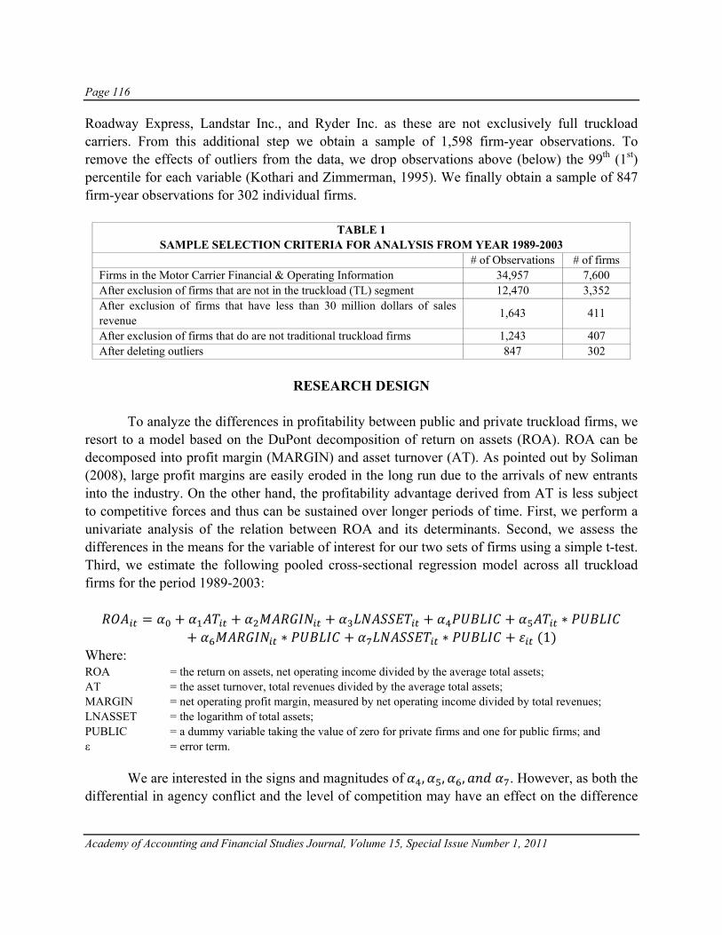
Page 116
Academy of Accounting and Financial Studies Journal, Volume 15, Special Issue Number 1, 2011
Roadway Express, Landstar Inc., and Ryder Inc. as these are not exclusively full truckload carriers. From this additional step we obtain a sample of 1,598 firm-year observations. To remove the effects of outliers from the data, we drop observations above (below) the 99th (1st) percentile for each variable (Kothari and Zimmerman, 1995). We finally obtain a sample of 847 firm-year observations for 302 individual firms.
TABLE 1 SAMPLE SELECTION CRITERIA FOR ANALYSIS FROM YEAR 1989-2003
# of Observations # of firms Firms in the Motor Carrier Financial & Operating Information 34,957 7,600 After exclusion of firms that are not in the truckload (TL) segment 12,470 3,352 After exclusion of firms that have less than 30 million dollars of sales revenue 1,643 411
After exclusion of firms that do are not traditional truckload firms 1,243 407 After deleting outliers 847 302
RESEARCH DESIGN
To analyze the differences in profitability between public and private truckload firms, we resort to a model based on the DuPont decomposition of return on assets (ROA). ROA can be decomposed into profit margin (MARGIN) and asset turnover (AT). As pointed out by Soliman (2008), large profit margins are easily eroded in the long run due to the arrivals of new entrants into the industry. On the other hand, the profitability advantage derived from AT is less subject to competitive forces and thus can be sustained over longer periods of time. First, we perform a univariate analysis of the relation between ROA and its determinants. Second, we assess the differences in the means for the variable of interest for our two sets of firms using a simple t-test. Third, we estimate the following pooled cross-sectional regression model across all truckload firms for the period 1989-2003:
1 Where: ROA = the return on assets, net operating income divided by the average total assets; AT = the asset turnover, total revenues divided by the average total assets; MARGIN = net operating profit margin, measured by net operating income divided by total revenues; LNASSET = the logarithm of total assets; PUBLIC = a dummy variable taking the value of zero for private firms and one for public firms; and ε = error term. We are interested in the signs and magnitudes of , , , . However, as both the differential in agency conflict and the level of competition may have an effect on the difference

Page 117
Academy of Accounting and Financial Studies Journal, Volume 15, Special Issue Number 1, 2011
in profitability between public and private firms, we make no prediction about the sign of each of these coefficients. To test whether public truckload firms grow more rapidly than their private counterparts, we estimate the following pooled cross-sectional regression model across all truckload firms for the period 1989-2003:
∆ ∆∆ ∆
2 Where:
GROWTH = the growth in revenues measured by the change in total revenues divided by the revenues from the previous period;
ΔOPERATING_RATIO = the change in the ratio of total expenses divided by total revenues; ΔROA = the change in the return on assets, net operating income divided by the
average total assets; LAGGROWTH = previous period’s growth; PUBLIC = a dummy variable taking the value of zero for private firms and one
for public firms; and ε = error term.
We are interested in the sign and magnitude of the coefficients on the interaction between our main independent variables and the dummy variable to distinguish private firms from their public counterparts. We include ΔOPERATING_RATIO as a determinant of growth as this ratio provides a measure of the change in the firm’s operating efficiency. The trucking industry is a competitive, capital intensive, and employee intensive industry so it is necessary to keep costs as low as possible. The firms with lower operating ratios are expected to grow at a more sustainable rate than the ones with higher operating ratios. With respect to the difference between public and private firms, the former are expected to be more efficient than the latter. Thus, we expect a higher operating ratio to have a more detrimental effect on the growth potential of public firms compared to the private ones.
RESULTS From both the descriptive statistics in Panel A and B of Table 2 and the test of difference in means in Table 4 we can show that on average, public truckload firms are more profitable (statistically significant difference of 3.16% in ROA), enjoy stronger profit margins (statistically significant difference of 1.6% in MARGIN), are larger, grow faster, and are more efficient in their operations than their private counterparts. These preliminary results provide early evidence that the owners of public trucking firms are more demanding than those of private firms and this leads the former to operate more efficiently than the latter.
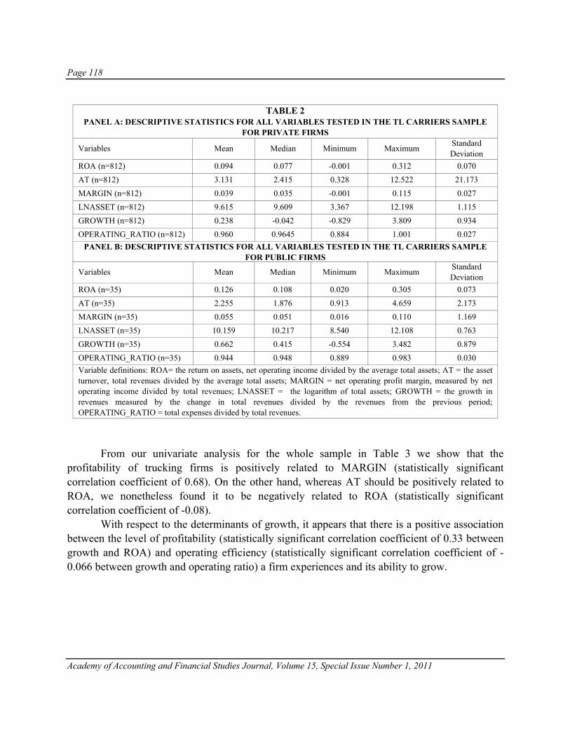
Page 118
Academy of Accounting and Financial Studies Journal, Volume 15, Special Issue Number 1, 2011
TABLE 2
PANEL A: DESCRIPTIVE STATISTICS FOR ALL VARIABLES TESTED IN THE TL CARRIERS SAMPLE FOR PRIVATE FIRMS
Variables Mean Median Minimum Maximum Standard Deviation
ROA (n=812) 0.094 0.077 -0.001 0.312 0.070 AT (n=812) 3.131 2.415 0.328 12.522 21.173 MARGIN (n=812) 0.039 0.035 -0.001 0.115 0.027 LNASSET (n=812) 9.615 9.609 3.367 12.198 1.115 GROWTH (n=812) 0.238 -0.042 -0.829 3.809 0.934 OPERATING_RATIO (n=812) 0.960 0.9645 0.884 1.001 0.027
PANEL B: DESCRIPTIVE STATISTICS FOR ALL VARIABLES TESTED IN THE TL CARRIERS SAMPLE FOR PUBLIC FIRMS
Variables Mean Median Minimum Maximum Standard Deviation
ROA (n=35) 0.126 0.108 0.020 0.305 0.073 AT (n=35) 2.255 1.876 0.913 4.659 2.173 MARGIN (n=35) 0.055 0.051 0.016 0.110 1.169 LNASSET (n=35) 10.159 10.217 8.540 12.108 0.763 GROWTH (n=35) 0.662 0.415 -0.554 3.482 0.879 OPERATING_RATIO (n=35) 0.944 0.948 0.889 0.983 0.030 Variable definitions: ROA= the return on assets, net operating income divided by the average total assets; AT = the asset turnover, total revenues divided by the average total assets; MARGIN = net operating profit margin, measured by net operating income divided by total revenues; LNASSET = the logarithm of total assets; GROWTH = the growth in revenues measured by the change in total revenues divided by the revenues from the previous period; OPERATING_RATIO = total expenses divided by total revenues.
From our univariate analysis for the whole sample in Table 3 we show that the profitability of trucking firms is positively related to MARGIN (statistically significant correlation coefficient of 0.68). On the other hand, whereas AT should be positively related to ROA, we nonetheless found it to be negatively related to ROA (statistically significant correlation coefficient of -0.08). With respect to the determinants of growth, it appears that there is a positive association between the level of profitability (statistically significant correlation coefficient of 0.33 between growth and ROA) and operating efficiency (statistically significant correlation coefficient of -0.066 between growth and operating ratio) a firm experiences and its ability to grow.

Page 119
Academy of Accounting and Financial Studies Journal, Volume 15, Special Issue Number 1, 2011
TABLE 3 SAMPLE CORRELATIONS (PEARSON)
Variables ROA AT MARGIN LNASSET GROWTH OPERATING_RATIO LAGGROWTH
ROA -0.08657 (0.0117)
0.68913 (<.0001)
0.26312 (<0.0001)
0.33802 (<.0001)
-0.68913 (<.0001)
-0.14205 (<.0001)
AT -0.38593 (<.0001)
-0.49905 (<.0001)
-0.13176 (<.0001)
0.38594 (<.0001)
-0.06394 (0.0630)
MARGIN 0.34828 (<0.0001)
0.06685 (0.0518)
-1.00000 (<.0001)
0.02492 0.4692
LNASSET
0.46774 (<0.0001)
-0.34830 (<0.0001)
0.24755 (<.0001)
GROWTH -0.06686 (0.0518)
-023067 (<.0001)
OPERATING_RATIO -0.0292 (0.4691)
LAGGROWTH Variable definitions: ROA= the return on assets, net operating income divided by the average total assets; AT = the asset turnover, total revenues divided by the average total assets; MARGIN = net operating profit margin, measured by net operating income divided by total revenues; LNASSET = the logarithm of total assets; GROWTH = the growth in revenues measured by the change in total revenues divided by the revenues from the previous period; OPERATING_RATIO = total expenses divided by total revenues.
TABLE 4
TESTS OF DIFFERENCES IN MEANS BETWEEN PUBLIC AND PRIVATE FIRMS
Variables Mean Private Mean Public Difference in means
(private-public) t-statistic p-value
ROA 0.0945 0.1261 -0.0316 -2.60 0.009 AT 3.131 2.255 0.876 2.37 0.01 MARGIN 0.04 0.0560 -0.016 -3.32 0.0009 LNASSET 9.615 10.1599 -0.544 -2.03 0.0429 GROWTH 0.238 0.662 -0.424 -2.64 0.008 OPERATING_RATIO 0.96 0.944 0.0160 3.32 0.0009 Variable definitions: ROA= the return on assets, net operating income divided by the average total assets; AT = the asset turnover, total revenues divided by the average total assets; MARGIN = net operating profit margin, measured by net operating income divided by total revenues; LNASSET = the logarithm of total assets; GROWTH = the growth in revenues measured by the change in total revenues divided by the revenues from the previous period; OPERATING_RATIO = total expenses divided by total revenues.
The results of multivariate analysis of the differences in profitability between public and private trucking firms are found in Table 5. The coefficients on both asset turnover and profit margin are positive and statistically significant as predicted by the literature on the drivers of firm’s profitability. However, the lack of statistical significance of the coefficient on the dummy PUBLIC shows that the ownership structure is not the major determinant of the difference in profitability between the two sets of firms. Moreover, none of the coefficients on the interaction variables are significant (AT*PUBLIC and MARGIN*PUBLIC). It therefore appears that the level of competition in the industry is so strong that it mitigates the effects related to the difference in ownership structure. We can therefore conclude that the truckload segment of the trucking industry is so competitive that survival in this segment mitigates the influence of the differences in the ownership structure on the performance of firms in the industry.
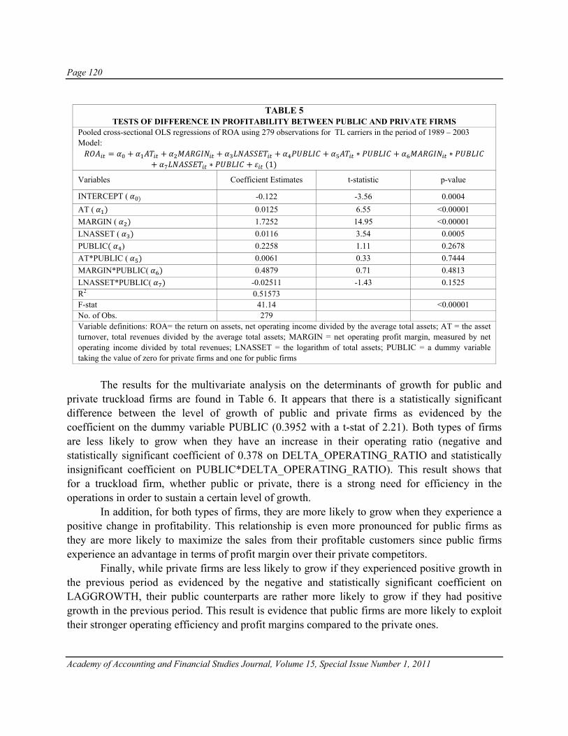
Page 120
Academy of Accounting and Financial Studies Journal, Volume 15, Special Issue Number 1, 2011
TABLE 5
TESTS OF DIFFERENCE IN PROFITABILITY BETWEEN PUBLIC AND PRIVATE FIRMS Pooled cross-sectional OLS regressions of ROA using 279 observations for TL carriers in the period of 1989 – 2003 Model:
1
Variables Coefficient Estimates t-statistic p-value
INTERCEPT ( -0.122 -3.56 0.0004 AT ( 0.0125 6.55 <0.00001 MARGIN ( 1.7252 14.95 <0.00001 LNASSET ( 0.0116 3.54 0.0005 PUBLIC ) 0.2258 1.11 0.2678 AT*PUBLIC ( 0.0061 0.33 0.7444 MARGIN*PUBLIC( 0.4879 0.71 0.4813 LNASSET*PUBLIC( -0.02511 -1.43 0.1525 R2 0.51573 F-stat 41.14 <0.00001 No. of Obs. 279 Variable definitions: ROA= the return on assets, net operating income divided by the average total assets; AT = the asset turnover, total revenues divided by the average total assets; MARGIN = net operating profit margin, measured by net operating income divided by total revenues; LNASSET = the logarithm of total assets; PUBLIC = a dummy variable taking the value of zero for private firms and one for public firms
The results for the multivariate analysis on the determinants of growth for public and private truckload firms are found in Table 6. It appears that there is a statistically significant difference between the level of growth of public and private firms as evidenced by the coefficient on the dummy variable PUBLIC (0.3952 with a t-stat of 2.21). Both types of firms are less likely to grow when they have an increase in their operating ratio (negative and statistically significant coefficient of 0.378 on DELTA_OPERATING_RATIO and statistically insignificant coefficient on PUBLIC*DELTA_OPERATING_RATIO). This result shows that for a truckload firm, whether public or private, there is a strong need for efficiency in the operations in order to sustain a certain level of growth. In addition, for both types of firms, they are more likely to grow when they experience a positive change in profitability. This relationship is even more pronounced for public firms as they are more likely to maximize the sales from their profitable customers since public firms experience an advantage in terms of profit margin over their private competitors. Finally, while private firms are less likely to grow if they experienced positive growth in the previous period as evidenced by the negative and statistically significant coefficient on LAGGROWTH, their public counterparts are rather more likely to grow if they had positive growth in the previous period. This result is evidence that public firms are more likely to exploit their stronger operating efficiency and profit margins compared to the private ones.
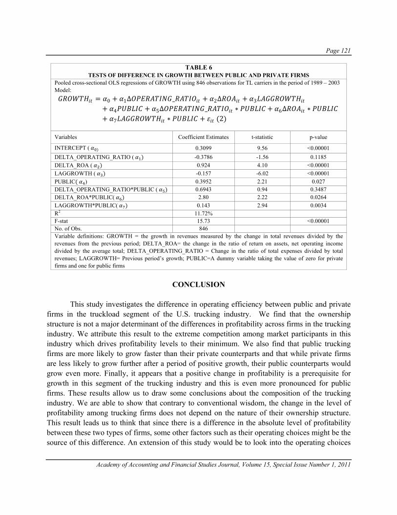
Page 121
Academy of Accounting and Financial Studies Journal, Volume 15, Special Issue Number 1, 2011
TABLE 6 TESTS OF DIFFERENCE IN GROWTH BETWEEN PUBLIC AND PRIVATE FIRMS
Pooled cross-sectional OLS regressions of GROWTH using 846 observations for TL carriers in the period of 1989 – 2003 Model:
Variables Coefficient Estimates t-statistic p-value
INTERCEPT ( 0.3099 9.56 <0.00001 DELTA_OPERATING_RATIO ( -0.3786 -1.56 0.1185 DELTA_ROA ( 0.924 4.10 <0.00001 LAGGROWTH ( -0.157 -6.02 <0.00001 PUBLIC ) 0.3952 2.21 0.027 DELTA_OPERATING_RATIO*PUBLIC ( 0.6943 0.94 0.3487 DELTA_ROA*PUBLIC( 2.80 2.22 0.0264 LAGGROWTH*PUBLIC( 0.143 2.94 0.0034 R2 11.72% F-stat 15.73 <0.00001 No. of Obs. 846 Variable definitions: GROWTH = the growth in revenues measured by the change in total revenues divided by the revenues from the previous period; DELTA_ROA= the change in the ratio of return on assets, net operating income divided by the average total; DELTA_OPERATING_RATIO = Change in the ratio of total expenses divided by total revenues; LAGGROWTH= Previous period’s growth; PUBLIC=A dummy variable taking the value of zero for private firms and one for public firms
CONCLUSION
This study investigates the difference in operating efficiency between public and private firms in the truckload segment of the U.S. trucking industry. We find that the ownership structure is not a major determinant of the differences in profitability across firms in the trucking industry. We attribute this result to the extreme competition among market participants in this industry which drives profitability levels to their minimum. We also find that public trucking firms are more likely to grow faster than their private counterparts and that while private firms are less likely to grow further after a period of positive growth, their public counterparts would grow even more. Finally, it appears that a positive change in profitability is a prerequisite for growth in this segment of the trucking industry and this is even more pronounced for public firms. These results allow us to draw some conclusions about the composition of the trucking industry. We are able to show that contrary to conventional wisdom, the change in the level of profitability among trucking firms does not depend on the nature of their ownership structure. This result leads us to think that since there is a difference in the absolute level of profitability between these two types of firms, some other factors such as their operating choices might be the source of this difference. An extension of this study would be to look into the operating choices
0 1∆ _ 2∆ 3
4 5∆ _ 6∆7 2

Page 122
Academy of Accounting and Financial Studies Journal, Volume 15, Special Issue Number 1, 2011
of public and private firms such as the decision to use company drivers or owner-operators or even the decision to buy or lease tractors and trailers to see if these factors make a difference.
REFERENCES ATA (2007-2008). American Trucking Associations Trucking and the Economy 2007-2008 Edition. ATRI (2004). The Trucking Industry from American Trucking Trends. Retrieved August 14, 2010, from
http://www.atri-online.org/industry/index.htm Banker, R., & Datar, S. M. (1989). Sensitivity, Precision, and Linear Aggregation of Signals for Performance
Evaluation . Journal of Accounting Research 27, 21-39. Feltham, G., & Xie, J. (1994). Performance Measure Congruity and Diversity in Multi-Task Principal/Agent
Relations. The Accounting Review Vol. 69 No. 3, 429-453. Holmstrom, B. (1979). Moral Hazard and Observability. Bell Journal of Economics 10, 74-91. Ittner, C., Larcker, D., & Rajan, M. (1997). The Choice of Performance Measures in Annual Bonus Contracts. The
Accounting Review Vol. 72 No. 2, 231-255. Jacobs, G. & O’Neill, C. (2003). On the Reliability (or Otherwise) of SIC Codes. European Business Review Vol. 15
No. 3, 164-169. Kothari, S. P., & Zimmerman, S. P. (1995). Price and Return Models . Journal of Accounting and Economics Vol.
20 (2), 155-192. Lockridge, D., editor (2005). The Rise of Truckload: Rebels with a Cause. Heavy Duty Trucking. Retrieved May 9,
2008, from: http://www.heavydutytrucking.com/2005/01/010a0501.asp Moore, T. G. (1993). "Trucking Deregulation," The Concise Encyclopedia of Economics. 1993. Library of
Economics and Liberty. Retrieved August 14, 2010 from the World Wide Web: http://www.econlib.org/library/Enc1/TruckingDeregulation.html
Soliman, M. (2008). The Use of DuPont Analysis by Market Participants. The Accounting Review .
Page 123
Academy of Accounting and Financial Studies Journal, Volume 15, Special Issue Number 1, 2011
A STUDY ON AUDIT PRICING AND MARKET ASSESSMENT OF RISK
Hema Rao, SUNY- Oswego
John MacDonald, SUNY- Oswego
ABSTRACT Audit pricing decisions of public accounting firms are not directly observable nor are the variables used in determining the audit fee. A number of research studies have, however, identified several accounting and corporate governance variables as significantly impacting the variability of audit fee of publicly traded firms. The riskiness of the audit client should be a consideration since there are legal and financial consequences for the auditor if the firm fails financially. Studies conducted in the U.S. on audit fees have not found systematic risk as a variable in audit fee determination of non-financial firms. This study finds that while the current systematic risk of the firm is significant in its impact on audit fees, this is true only for firms with relatively little regulation. Firms with heavier regulation do not show impact of current systematic risk, but only changes in systematic risk (from the prior year.) These regulated firms include banks, insurance companies, media and telecommunications firms. The findings overall suggest that audit committees and management need to be aware of how restructuring of assets and financing and risk management, such as hedging will impact on the accounting risk and costs to the firm.
INTRODUCTION This research investigates auditee systematic risk in audit pricing decisions. A number of empirical studies present evidence on audit fee pricing and identify many factors that impact such fee. Cobbin (2002) has an extensive review of studies on audit fees. The seminal Simunic study (1980) used US data and since then many international studies have replicated the basic regression model that include several variables. Most studies find that differences in audit fee are explained by client attributes like size, audit effort and audit risk. Audit risk is theoretically defined as a combination of inherent risk, control risk and detection risk and is expressed as
AR = IR X CR X DR
Where, AR= Audit risk, IR = Inherent risk, CR = Control risk and DR = Detection risk (Arens, Elder, Beasley, 2009). Inherent risk is client specific and includes many macro and micro factors. The purpose of this study is to determine if systemic risk of a firm (as measured
Page 124
Academy of Accounting and Financial Studies Journal, Volume 15, Special Issue Number 1, 2011
by the market β) affects audit pricing decisions. We believe that the inclusion of β as one of the components in inherent risk may be appropriate after considering some of the micro and macro factors in the KPMG audit model (Bell, Mars, Solomon, & Thomas, 1997). Effect of Client’s Risk on Audit Fees As defined in the model above, control risk is the probability of the client’s internal control system failing to prevent financial statement misstatements exceeding the auditor’s predetermined assessment of such risk. In the era of the implementation of internal control reporting requirements following the passage of Sarbanes-Oxley (SOX), the components of internal control suggested by the 2004 Committee of Sponsoring Organizations of the Treadway Commission (COSO) framework are considered in the assessment of internal control risk. Abbott et al (2003) consider the quality of audit committees (COSO mandated corporate governance factors) in predicting audit fees. Raghunathan and D. V. Rama (2006) report that the audit fee in the year 2004 (internal control disclosures required by Section 404 of the SOX) was significantly higher than in the prior year. Huang et al (2009) have considered audit fee differences in pre-and post-SOX continuing and initial audits. They report that the initial fee discounts seen in 2001 Big 4 audits are not available in the post-Sox 2006 audit fee. Detection risk deals with auditor specific issues in performing the audit. Some studies have considered differences in quality of Big 4 vs. Non-Big 4 audit fees (Simunic 1980) and auditor specialization (Cahan et al 2008) in audit fee determination. Healy (2005) suggests a key role for auditors as intermediaries in the capital markets for reducing investor information risk. He suggests that audit pricing must provide for higher quality audits that may reduce the risk of fraud. He suggests that this type of high quality audit work may even reduce litigation risk for auditors. Role of Systemic Risk β is a market risk indicator of a stock’s volatility in relation to the market’s volatility and since auditors play a role in the capital markets’ certification processes, β may well affect in determining audit fee. Just like an investor, an auditor accepts several clients from a portfolio of firms and hence has a selection problem. According to Markowitz (1952), systematic risk of a firm (audit client) should affect the selection problem. Various liquidity, profitability and leverage ratios (Cobbin 2002) used to estimate audit risk may also contain some unsystematic risk elements that may be somewhat biased. Capital Asset Pricing Models developed by Sharpe (1964) and Lintner (1965) and Mossin (1964) suggest that the appropriate measure for determining a firm’s systematic risk is β. Betas (β) may better capture client risk in any audit pricing model, since it reflects the firm’s business risk as viewed in the financial markets. β is estimated using stock market returns and an individual firm .
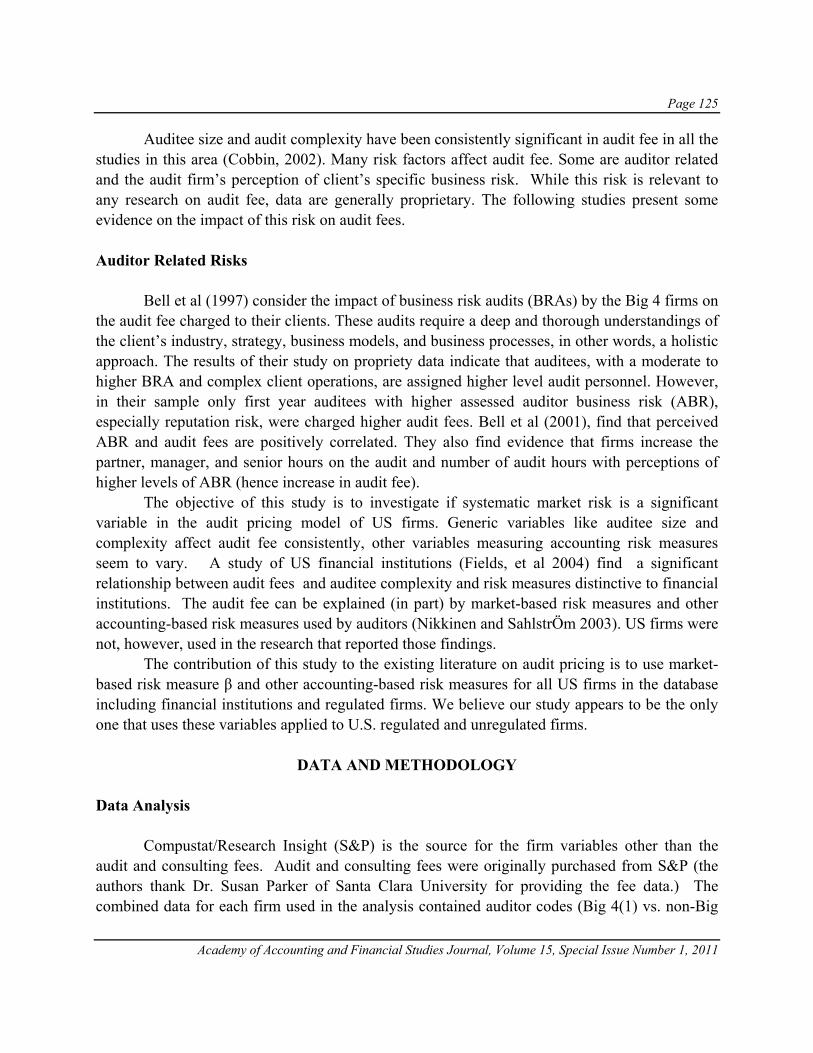
Page 125
Academy of Accounting and Financial Studies Journal, Volume 15, Special Issue Number 1, 2011
Auditee size and audit complexity have been consistently significant in audit fee in all the studies in this area (Cobbin, 2002). Many risk factors affect audit fee. Some are auditor related and the audit firm’s perception of client’s specific business risk. While this risk is relevant to any research on audit fee, data are generally proprietary. The following studies present some evidence on the impact of this risk on audit fees. Auditor Related Risks Bell et al (1997) consider the impact of business risk audits (BRAs) by the Big 4 firms on the audit fee charged to their clients. These audits require a deep and thorough understandings of the client’s industry, strategy, business models, and business processes, in other words, a holistic approach. The results of their study on propriety data indicate that auditees, with a moderate to higher BRA and complex client operations, are assigned higher level audit personnel. However, in their sample only first year auditees with higher assessed auditor business risk (ABR), especially reputation risk, were charged higher audit fees. Bell et al (2001), find that perceived ABR and audit fees are positively correlated. They also find evidence that firms increase the partner, manager, and senior hours on the audit and number of audit hours with perceptions of higher levels of ABR (hence increase in audit fee). The objective of this study is to investigate if systematic market risk is a significant variable in the audit pricing model of US firms. Generic variables like auditee size and complexity affect audit fee consistently, other variables measuring accounting risk measures seem to vary. A study of US financial institutions (Fields, et al 2004) find a significant relationship between audit fees and auditee complexity and risk measures distinctive to financial institutions. The audit fee can be explained (in part) by market-based risk measures and other accounting-based risk measures used by auditors (Nikkinen and SahlstrÖm 2003). US firms were not, however, used in the research that reported those findings. The contribution of this study to the existing literature on audit pricing is to use market-based risk measure β and other accounting-based risk measures for all US firms in the database including financial institutions and regulated firms. We believe our study appears to be the only one that uses these variables applied to U.S. regulated and unregulated firms.
DATA AND METHODOLOGY Data Analysis Compustat/Research Insight (S&P) is the source for the firm variables other than the audit and consulting fees. Audit and consulting fees were originally purchased from S&P (the authors thank Dr. Susan Parker of Santa Clara University for providing the fee data.) The combined data for each firm used in the analysis contained auditor codes (Big 4(1) vs. non-Big

Page 126
Academy of Accounting and Financial Studies Journal, Volume 15, Special Issue Number 1, 2011
4(0)), annual β, exchange on which the common stock traded, auditor fees, auditor consulting fees and data on firm sales, current assets, total assets and total liabilities for the years 2000 and 2001. A log transformation was used for the asset value variable. Ratios were also computed for measures of liquidity (current-assets-to-total- assets) and debt load (total-liabilities-to-total-assets). The initial sample had a total of 2373 firms. The sample was divided into two classes based on the SIC code: (1) regulated (banks, insurance companies, telecommunications and media companies and (2) unregulated. This categorization provided 1899 “unregulated” firms and 474 “regulated” firms. Forty-six firms were removed for either missing data or because the firm data included outliers beyond four sigmas (standard deviations) from the variable mean. Following the removal of the 44 outliers, the final dataset had 2329 total observations containing 1883 unregulated firms and 446 regulated firms. The descriptive statistics relating to firm descriptors are provided in Table 1.
Table 1 Descriptive Statistics for Data
ALL N= 2329 Regulated N=446 UnRegulated
N=1883 Variable/Statistic Mean (Std dev ) Mean (Std dev ) Mean (Std dev )
Β2001 .7943 (1.1267 ) .3829 (.3722) .8918 (.7305) Β Change from 2000 to 2001 .1618 (.7284 ) -.0449 (.2576) .2107 (.7926)
Total Sales 2001 $2.34b 8.7b) $2.96b ($8.39b) $2.2b ($8.77b) Total Current Assets $.602b ($2.18b) $.343b ($1.56b) $.663b ($2.3b)
Total Assets $6.21b ($35.0b) $17.3b ($67.1b) $3.57b ($20.2b) Total Current Liabilities $.484b ($1.99b) $.378b ($1.59b) $.509b ($2.07b)
Total Liabilities $5.01b ($1.01b) $15.6b ($63.4b) $2.49b ($17.4b) Audit Fees (000) $667.5k ($1493.4k) $720.57k ( $654.92k ($1464k)
IS Consulting Fees (000) $ 81.17k ($611.73k) 80.807k (530.727k) $81.257k ($629.53k) Total Liabilities to Total Assets .5628 (.2925) .8407 (.1432) .4969 (.2799) Current Assets to Total Assets .3631 (.2991 ) .0377 (.1120) .4402 (.2769)
ALL N= 2329 Regulated N=446 UnRegulated N=1883 From the descriptive statistics for the sample, it is clear that the regulated firms have a different profile than the firms with less regulation. The systematic risk for the regulated firms is .3829, considerably below the market level of 1 and the mean of the unregulated firms. When we look at the change in β across the period of 2000 to 2001, regulated firms actually saw an average decrease in systematic risk, while unregulated firms saw a modest increase (.2107) on average. This could be indicative of the recessionary and political (9/11, terrorism) events of this time period in which many investors would have moved to what they perceived were less risky firms (i.e. regulated firms.)

Page 127
Academy of Accounting and Financial Studies Journal, Volume 15, Special Issue Number 1, 2011
At least on average, the regulated firms had a lower amount of current assets but were much larger firms, using much more debt. This would certainly be true of regulated financial institutions. Average sales and consulting fees for the two subsets are, however, rather close in size. In the research sample, 384 four-digit SIC codes were represented. Table 2 provides a view of the SIC code ranges and lists those individual code values with twenty-five or more firms. Of the 384 different SIC codes, 303 codes were represented by only one firm in the sample, so there is a rather diverse sample with respect to industries.
Table 2 SIC Codes
SIC Code Description Number of Firms Range 100-9997 2329 1389 OIL & GAS FIELD SERVICES 70 2673 PLASTIC, FOIL,COATED PAPER BAGS 25 2891 ADHESIVES & SEALANTS 186 3357 DRAWING, INSULATING NONFERROUS WIRE 32 3490 MISC. FABRICATED METAL PRODUCTS 32 3590 MISC. INDUSTRIAL COMMERCIAL MACHINERY & EQUIPMENT 113 3695 MAGNETIC, OPTIC RECORDING MEDIA 129 3790 MISC. TRANSPORTATION EQUIPMENT 38 3873 WATCHES, CLOCKS, AND PARTS 110 4899 COMMUNICATION SERVICES 76 5094 JEWELRY & WATCHES - WHOLESALE 38 5990 RETAIL STORES 34 6798 REAL ESTATE INVESTMENT TRUSTS 110 7389 BUSINESS SERVICES 271 8093 SPECIAL OUTPATIENT FACILITY 32 8742 MANAGEMENT CONSULTING SERVICES 60 4931 ELECTRICAL & OTHER SERVICE COMB. 64 6099 FUNCTIONS RELATED TO DEP BANKING 275
Methodology The extant literature has shown that audit fees are impacted by liquidity (typically measured as current assets/total assets), reliance on debt (measured as total liabilities to total assets or a lognormal version), firm size (usually measured as the log of the assets or log of sales), consulting fees, auditor, the exchange on which the firm’s common stock trades, and systematic risk (measured as a recent or lag β.) Turpen (1990) classified his sample firms on the basis of the exchanges on which the sample firm stocks were traded but did not include them as a variable in his analysis. Based on prior research stock exchanges were not included in the regression models examined in the current study.
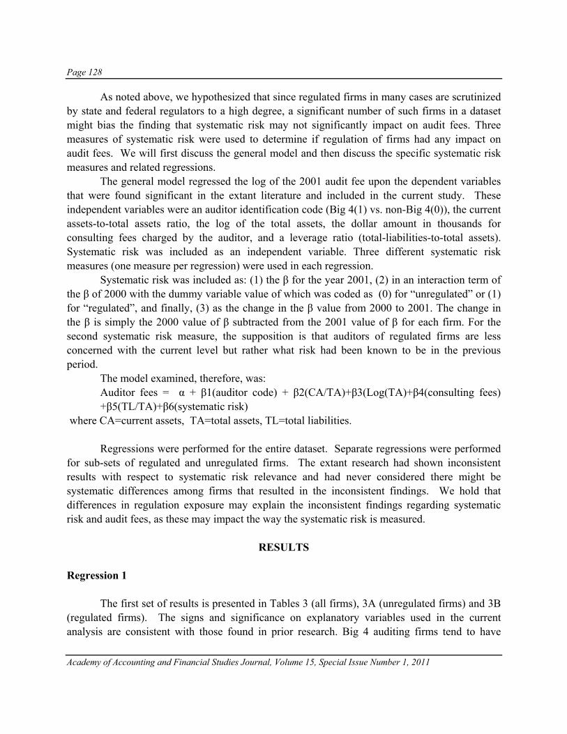
Page 128
Academy of Accounting and Financial Studies Journal, Volume 15, Special Issue Number 1, 2011
As noted above, we hypothesized that since regulated firms in many cases are scrutinized by state and federal regulators to a high degree, a significant number of such firms in a dataset might bias the finding that systematic risk may not significantly impact on audit fees. Three measures of systematic risk were used to determine if regulation of firms had any impact on audit fees. We will first discuss the general model and then discuss the specific systematic risk measures and related regressions. The general model regressed the log of the 2001 audit fee upon the dependent variables that were found significant in the extant literature and included in the current study. These independent variables were an auditor identification code (Big 4(1) vs. non-Big 4(0)), the current assets-to-total assets ratio, the log of the total assets, the dollar amount in thousands for consulting fees charged by the auditor, and a leverage ratio (total-liabilities-to-total assets). Systematic risk was included as an independent variable. Three different systematic risk measures (one measure per regression) were used in each regression. Systematic risk was included as: (1) the β for the year 2001, (2) in an interaction term of the β of 2000 with the dummy variable value of which was coded as (0) for “unregulated” or (1) for “regulated”, and finally, (3) as the change in the β value from 2000 to 2001. The change in the β is simply the 2000 value of β subtracted from the 2001 value of β for each firm. For the second systematic risk measure, the supposition is that auditors of regulated firms are less concerned with the current level but rather what risk had been known to be in the previous period. The model examined, therefore, was: Auditor fees = α + β1(auditor code) + β2(CA/TA)+β3(Log(TA)+β4(consulting fees)
+β5(TL/TA)+β6(systematic risk) where CA=current assets, TA=total assets, TL=total liabilities. Regressions were performed for the entire dataset. Separate regressions were performed for sub-sets of regulated and unregulated firms. The extant research had shown inconsistent results with respect to systematic risk relevance and had never considered there might be systematic differences among firms that resulted in the inconsistent findings. We hold that differences in regulation exposure may explain the inconsistent findings regarding systematic risk and audit fees, as these may impact the way the systematic risk is measured.
RESULTS Regression 1 The first set of results is presented in Tables 3 (all firms), 3A (unregulated firms) and 3B (regulated firms). The signs and significance on explanatory variables used in the current analysis are consistent with those found in prior research. Big 4 auditing firms tend to have

Page 129
Academy of Accounting and Financial Studies Journal, Volume 15, Special Issue Number 1, 2011
higher fees. Higher fees are associated with larger firms, firms with larger debt ratios, and use of consulting services. Firms with higher current assets as a proportion of their asset structure also tend to have higher auditor fees. While cash would be a very low risk current asset, receivables and certain types of inventory could be viewed as risky, especially if their respective periods (collection and inventory) were longer than the payables period for the firm.
Table 3 Regression 1 Systematic Risk = 2001 β All Firms in Sample
Adjusted-R2 .6202 N=2328 F-statistic(significance) 634.44(~0)* P-Values of Independent Variables↓ α (intercept) -2.2787 5.2675E-143* Auditor Code (Big 4 =1, Non Big 0) .2099 2.5598E-16* CA/TA .5591 2.63069E-82* Log(TA) .4860 ~0* Consulting Fees (000s) 6.50309E-05 2.08569E-10* TL/TA .0982 .0001632* 2001 β .0152 .006873** * p<.001 **p<.01 ***p<.10
Table 3A Regression 1 Systematic Risk = 2001 β
Unregulated Firms in Sample Adjusted-R2 .6480 N=1882 F-statistic(significance) 578.22 (~0)* P-Values of Independent Variables↓ α (intercept) -2.1158 7.5E-108* Auditor Code (Big 4 =1, Non Big 0) .05438 .090252*** CA/TA .42158 1.36E-46* Log(TA) .4877 ~0* Consulting Fees (000s) 5.51948E-05 1.11E-07* TL/TA .2387 4.18E-20* 2001 β .0118 .027736*** * p<.001 **p<.01 ***p<.10
Table 3B Regression 1 Systematic Risk = 2001 β
Regulated Firms in Sample Adjusted-R2 .7697 N=446 F-statistic(significance) 248.85 (7.97E-138)* P-Values of Independent Variables↓ α (intercept) -2.3667 1.0231E-38* Auditor Code(Big 4 =1, Non Big 0) .1742 1.24408E-06* CA/TA .8315 4.0721E-12* Log(TA) .5631 2.1588E-104* Consulting Fees (000s) 4.04615E-05 .080923*** TL/TA -.8072 7.74228E-16* 2001 β .0118 .737723 * p<.001 **p<.01 ***p<.10

Page 130
Academy of Accounting and Financial Studies Journal, Volume 15, Special Issue Number 1, 2011
For all regressions there is consistency in the adjusted R2 values, with values ranging from .62 to .77. F-statistics also consistently show significant values for the overall models. These regressions use the 2001 β as a measure of systematic risk. The current year β is significant and the variable sign is positive for the entire dataset, and for the subset of unregulated firms (Table 3A). Regulated firms (Table 3B) do not show the current beta level to be a significant variable in audit fee determination. One of the foremost functions of regulation is to reduce risk and ensure stability in certain industries. An interpretation of the results for the first set of regressions and the descriptive statistics is that regulated firms are viewed as having lower risk at any point in time than most unregulated firms, so there is more risk to auditors from challenges on firms with higher systematic risk. What would be of more concern to auditors with regard to regulated firms might be changes in the level of systematic risk, which is subject to more monitoring. Use of Dummy Variables and Prior Year β Regression 2 Table 4 shows the results of the second regression in which the systematic risk measure (β) (β2000) is multiplied by 1 for regulated firms and 0 for unregulated firms. This (β2000*1) variable has a negative sign and is highly significant. The negative sign indicates that current year (2001) fees will be lower when the systematic risk of the previous year (β 2000) was higher than the one for the current year (β 2001). Consequently, current year fees will fall when the systematic risk was higher in the previous year. This suggests that when beta increases from one year to the next, fees may also increase. In other word, for regulated firms, there is greater concern for changes in systematic risk, rather than the level of risk.
Table 4 Regression 2 Systematic Risk = Interaction term
All Firms in Sample Adjusted-R2 .6336 N=2329 F-statistic(significance) 56.6499(~0)* P-Values of Independent Variables↓ α (intercept) -2.3965 8.9455E-158* Auditor Code(Big 4 =1, Non Big 0) .2054 3.33846E-16* CA/TA .5309 6.95967E-78* Log(TA) .5032 ~0* Consulting Fees (000s) 5.95562E-05 3.26733E-09* TL/TA .1255 1.12808E-06* Interaction Beta 2000/Regulation -.2739 4.1404E-21* * p<.001 **p<.01 ***p<.10
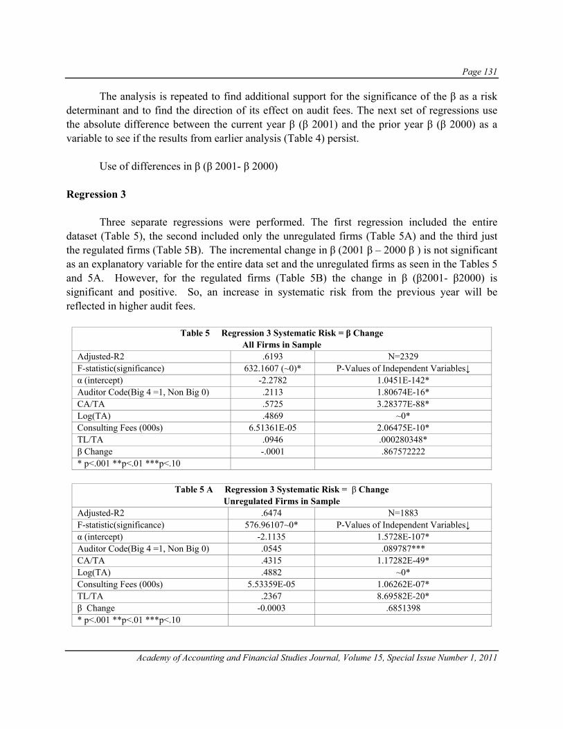
Page 131
Academy of Accounting and Financial Studies Journal, Volume 15, Special Issue Number 1, 2011
The analysis is repeated to find additional support for the significance of the β as a risk determinant and to find the direction of its effect on audit fees. The next set of regressions use the absolute difference between the current year β (β 2001) and the prior year β (β 2000) as a variable to see if the results from earlier analysis (Table 4) persist. Use of differences in β (β 2001- β 2000) Regression 3 Three separate regressions were performed. The first regression included the entire dataset (Table 5), the second included only the unregulated firms (Table 5A) and the third just the regulated firms (Table 5B). The incremental change in β (2001 β – 2000 β ) is not significant as an explanatory variable for the entire data set and the unregulated firms as seen in the Tables 5 and 5A. However, for the regulated firms (Table 5B) the change in β (β2001- β2000) is significant and positive. So, an increase in systematic risk from the previous year will be reflected in higher audit fees.
Table 5 Regression 3 Systematic Risk = β Change All Firms in Sample
Adjusted-R2 .6193 N=2329 F-statistic(significance) 632.1607 (~0)* P-Values of Independent Variables↓ α (intercept) -2.2782 1.0451E-142* Auditor Code(Big 4 =1, Non Big 0) .2113 1.80674E-16* CA/TA .5725 3.28377E-88* Log(TA) .4869 ~0* Consulting Fees (000s) 6.51361E-05 2.06475E-10* TL/TA .0946 .000280348* β Change -.0001 .867572222 * p<.001 **p<.01 ***p<.10
Table 5 A Regression 3 Systematic Risk = β Change
Unregulated Firms in Sample Adjusted-R2 .6474 N=1883 F-statistic(significance) 576.96107~0* P-Values of Independent Variables↓ α (intercept) -2.1135 1.5728E-107* Auditor Code(Big 4 =1, Non Big 0) .0545 .089787*** CA/TA .4315 1.17282E-49* Log(TA) .4882 ~0* Consulting Fees (000s) 5.53359E-05 1.06262E-07* TL/TA .2367 8.69582E-20* β Change -0.0003 .6851398 * p<.001 **p<.01 ***p<.10

Page 132
Academy of Accounting and Financial Studies Journal, Volume 15, Special Issue Number 1, 2011
This outcome supports the results in Table 4 which indicate that an increase in β may be associated with a corresponding increase in the audit fees. The auditor may perceive a change from a lower level of β in 2000 to a higher β 2001 as an indicator of higher risk and compensate for it by charging higher audit fees. In addition to the perceived higher audit risk due to increases in β, and as stated earlier, the fees may include the effects of regulatory issues that impact on the financial statement audit resulting in additional audit hours and higher level audit personnel (higher billable audit hours) involvement in the audit. As in prior results the R2 ranged from .6193 to .7730 and the F statistics for all the models are robust and very significant (Table 5, R2 .6193 F 632.16, Table 5 A R2 .6474: F 576.96, Table 5 B R2 .7730: F 253.63). The variables used were significant and the only difference in results was for β which was not significant in the whole data set as well as in the unregulated firm subset regressions. Additional explanations for the results were provided in earlier paragraphs.
Table 5 B Regression 3 Systematic Risk = β Change
Regulated Firms in Sample Adjusted-R2 .7730 N=446 F-statistic(significance) 253.6266~0* P-Values of Independent Variables↓ α (intercept) -2.4519 8.29159E-41* Auditor Code (0, (Big 4 =1, Non Big 0) .1752 8.29159E-07*
CA/TA .8546 4.85754E-13* Log(TA) .5686 6.2184E-113 Consulting Fees (000s) 3.91242E-05 .088395072*** TL/TA -.7576 2.50859E-14* β Change .1235 .010404*** * p<.001 **p<.01 ***p<.10
LIMITATIONS The dataset used in the empirical research restricts the findings in the study to the two years of available data used in the current investigation. Further regulations in corporate governance have been instituted since then. The levels of regulation between regulated and unregulated firms may have changed somewhat due to these additional compliance measures applicable to both sets of firms. More current data may capture all the effects of the additional regulation and hence, the systemic risk implications may need to be reassessed to study any potential changes in audit fees, if any.
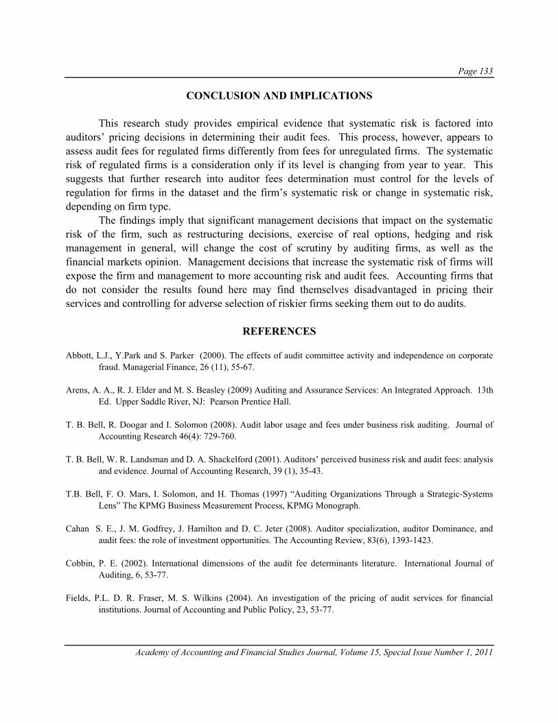
Page 133
Academy of Accounting and Financial Studies Journal, Volume 15, Special Issue Number 1, 2011
CONCLUSION AND IMPLICATIONS This research study provides empirical evidence that systematic risk is factored into auditors’ pricing decisions in determining their audit fees. This process, however, appears to assess audit fees for regulated firms differently from fees for unregulated firms. The systematic risk of regulated firms is a consideration only if its level is changing from year to year. This suggests that further research into auditor fees determination must control for the levels of regulation for firms in the dataset and the firm’s systematic risk or change in systematic risk, depending on firm type. The findings imply that significant management decisions that impact on the systematic risk of the firm, such as restructuring decisions, exercise of real options, hedging and risk management in general, will change the cost of scrutiny by auditing firms, as well as the financial markets opinion. Management decisions that increase the systematic risk of firms will expose the firm and management to more accounting risk and audit fees. Accounting firms that do not consider the results found here may find themselves disadvantaged in pricing their services and controlling for adverse selection of riskier firms seeking them out to do audits.
REFERENCES Abbott, L.J., Y.Park and S. Parker (2000). The effects of audit committee activity and independence on corporate
fraud. Managerial Finance, 26 (11), 55-67. Arens, A. A., R. J. Elder and M. S. Beasley (2009) Auditing and Assurance Services: An Integrated Approach. 13th
Ed. Upper Saddle River, NJ: Pearson Prentice Hall. T. B. Bell, R. Doogar and I. Solomon (2008). Audit labor usage and fees under business risk auditing. Journal of
Accounting Research 46(4): 729-760. T. B. Bell, W. R. Landsman and D. A. Shackelford (2001). Auditors’ perceived business risk and audit fees: analysis
and evidence. Journal of Accounting Research, 39 (1), 35-43. T.B. Bell, F. O. Mars, I. Solomon, and H. Thomas (1997) “Auditing Organizations Through a Strategic-Systems
Lens” The KPMG Business Measurement Process, KPMG Monograph. Cahan S. E., J. M. Godfrey, J. Hamilton and D. C. Jeter (2008). Auditor specialization, auditor Dominance, and
audit fees: the role of investment opportunities. The Accounting Review, 83(6), 1393-1423. Cobbin, P. E. (2002). International dimensions of the audit fee determinants literature. International Journal of
Auditing, 6, 53-77. Fields, P.L. D. R. Fraser, M. S. Wilkins (2004). An investigation of the pricing of audit services for financial
institutions. Journal of Accounting and Public Policy, 23, 53-77.

Page 134
Academy of Accounting and Financial Studies Journal, Volume 15, Special Issue Number 1, 2011
Hamada, R., (1972). The effects of a firm’s capital structure on the systematic risk of common stocks. Journal of Finance, 27, 435-452.
Healy, P. M.,(2005) The Challenges Facing Auditors and Analysts in U.S. Capital Markets. Retrieved July 15, 2008
from http://newman.baruch.cuny.edu/DIGITAL/saxe/saxe_2005/healy_05.html. Hua-Wei H., K. Raghunandan, and D. V. Raman (2009). Audit fees for initial audit engagements before and after
SOX. Auditing: A Journal of Practice & Theory 25 (1):171-190. Lintner, J. (1965). The valuation of risk assets and the selection of risky investments in stock portfolios and capital
budgets. Review of Economics and Statistics, 47, 13-37. Markowitz, H. (1952). Portfolio selection. Journal of Finance , 7, 77-91. Mossin, J. (1966). Equilibrium in a capital asset market. Econometrica, 34, 768-783. Nikkinen. J. and P. SahlstrÖm (2003). Do auditors assess the systematic market risk in their audit decisions?
International Evidence. Advances in Accounting, 20, 233-244. Raghunandan, K and D. V. Rama. (2006). SOX section 404 material weakness disclosures and audit fees. Auditing:
A Journal of Practice & Theory, 25 (1), 99-114. Sharpe, W.F. (1964). Capital asset prices: a theory of market equilibrium under conditions of risk. Journal of
Finance, 19, 425-442. Simunic, D. A. (1980). The pricing of audit services: theory and evidence. Journal of Accounting Research, 18(1),
161-190. Turpen, R. A., (1990). Differential pricing on auditors’ initial engagements: further evidence. Auditing: A Journal
of Practice & Theory, 9(2), 60-76.

Page 135
Academy of Accounting and Financial Studies Journal, Volume 15, Special Issue Number 1, 2011
LIQUIDITIY AND FINANCIAL LEVERAGE RATIOS: THEIR IMPACT ON COMPLIANCE WITH
INTERNATIONAL FINANCIAL REPORTING STANDARDS (IFRS)
Rodiel C. Ferrer, De La Salle – Manila, Philippines Glenda J. Ferrer, University of Rizal System, Philippines
ABSTRACT This paper investigates how the liquidity and leverage ratios exert significant effect on the degree of compliance with International Financial Reporting Standard disclosure as measured by Balance Sheet and Income Statement of Publicly Listed Corporations. The researcher analyzed the effects of current ratio, quick ratio, debt equity ratio and interest coverage ratio on compliance with IFRS. The compliance audit output was used by the author to calculate the financial statement disclosure index using a dichotomous procedure to score each of the company indices. This study covered 100 publicly listed corporations in the Philippines from different industries out of the 244 PLCs. The companies belong to different sectors / industries such as Financials, Industrial, Holding Firms, Property, Services, and Mining and Oil. Published annual reports of the aforesaid companies have been used as a secondary source. Disclosure indices were constructed from 475 items of Balance Sheet disclosure checklist and 263 items of Income Statement disclosure checklist based on the compliance audit consistent with the International Financial Reporting Standard (IFRS) Report Checklist. Using multiple regression analysis, the author regressed each of balance sheet index, income statement index and total of income statement – balance sheet indices, against liquidity ratios and financial leverage ratios such as current ratio, quick ratio, debt ratio and interest coverage ratio. Finding suggests that none of the indices exert a significant effect on the financial variables cited based on the computed t-statistics whose p-values are greater than the level of significance (α = 0.05). Therefore, the null hypothesis, that liquidity and financial leverage have no effect on IFRS when the latter is expressed in terms of Balance Sheet and Income Statement indices, is accepted.

Page 136
Academy of Accounting and Financial Studies Journal, Volume 15, Special Issue Number 1, 2011
INTRODUCTION A recent and important trend in financial reporting and disclosure regulation is the increasingly widespread adoption of uniform financial reporting standards by stock exchanges and accounting standards bodies from different countries. These uniform standards are labeled International Financial Reporting Standards (IFRS) and their stated goal is to achieve global “harmonization” and “convergence” of financial reporting rules and regulations. International Financial Reporting Standards (IFRS) are accounting rules issued by the International Accounting Standards Board (IASB). In contrast to local accounting rules (domestic GAAP) that differ across markets and countries, IFRS are a set of uniform rules that, in theory, apply in the same way to all public companies in markets that adopt the standards. IFRS are principles-based reporting standards that attempt to cover a broad range of economic conditions, transactions, activities or events. Over 100 countries have recently moved to IFRS reporting or decided to require the use of these standards in the near future, and even the U.S. is considering allowing U.S. firms to prepare their financial statements in accordance with IFRS. While the overall impact of IFRS is still to be determined, promoters of IFRS often argue that uniform global standards are obviously superior to disparate, and in many cases competing, standards across markets. However, the optimality of a single set of mandated global financial reporting rules, let alone the specific uniform rules contained in the current IFRS, is not obvious (e.g., Dye and Sunder, 2001). While mandatory uniform rules and regulations may provide aggregate economic benefits, the individual and aggregate costs of uniform global regulations on firms, investors, and other stakeholders are often not recognized nor discussed. In particular, IFRS draw heavily on the current financial reporting regulations of countries and markets that are geared toward outside capital providers. Moreover, these advanced countries have institutional infrastructures that complement the type of reporting regulations that have developed in these markets. Therefore, it is far from clear that IFRS will be superior or even effective in countries that have different capital-market paradigms and lack the necessary institutional infrastructures to support the effective application and enforcement of the uniform global standards. Despite the importance of corporate transparency as a recurring policy issue, there is (i) limited research on the costs and benefits of financial reporting and disclosure regulation, (ii) few attempts to systematically organize the key economic principles of and empirical findings on this type of regulation, and (iii) little guidance on important unanswered questions about the economic consequences of regulating financial reporting and corporate disclosure (Leuz, 2008). This paper evaluates how the liquidity and leverage ratios exert significant effect on the degree of compliance with International Financial Reporting Standard disclosure as measured by Balance Sheet and Income Statement of Publicly Listed Corporations.

Page 137
Academy of Accounting and Financial Studies Journal, Volume 15, Special Issue Number 1, 2011
CONCEPTUAL FRAMEWORK Agency theory portrays the relationship of principal and agent. In agency relationship, principals (shareholders) hire agents (managers) to manage business operations and entrust to them the decision-making authority. In corporations, a central problem exists concerning shareholders’ interest: top management does not always act in the best interest of shareholders. As a result, tension takes place between two parties since managers first serve their interest: either in the manner of shirking, which is lack of attention for maximizing shareholders returns in the corporate governance context, or self opportunistic behavior, by accruing wealth meant for themselves instead for shareholders. Information asymmetry occurs when managers have easy and better access to information against shareholders (Lee and Choi, 2002). Managers, in this instance, have the capacity to control and suppress relevant information from stakeholders. Therefore, managers have the discretion on the level of disclosed information that could affect decisions made by shareholders. With a high level of information asymmetry, stakeholders could not avail the incentives, the resources, and the access to information in overseeing management’s actions (Richardson, 2000). This heightened the presence of information asymmetry as a necessary requirement for earnings management to take place (Dye, 1988; as cited by Richardson, 2000) since the environmental conditions surrounding the firm provides opportunities for managers to manipulate information presented to the stakeholders. Stakeholders estimate the value of a company not only in terms of financial measure but also by its nonfinancial and strategic performance. Annual reports are now seen as the primary source of corporate information disclosure. Additionally, annual reports may also provide voluntary information. The efficiency of the disclosure process is dependent upon the needs of the stakeholders and of the interests of the management of the corporation (Debreceny, Gray, Mock, 2001). Roberts (2004) explained that agency theory has a number of related manifestations. As with neoclassical economics, the basic unit of analysis is taken as the ‘individual’ who is preoccupied with maximizing or at least satisfying utility, conceived typically in terms of a trade-off between work and leisure. It is this combination of assumed autonomy and self-interested motivation that creates the problems within agency relationships, the relationship between a principal and those employed as ‘agents’ to serve their interests. Kusumawati and Riyanto (2005) in their research have proven that good corporate governance disclosures in addition to corporate governance variables are important to investors. Investors are very eager and willing to pay at a higher share price to companies that both practice and disclose governance related information in the annual report. Bhat et al (2006) added that investors use governance related disclosures in examining the quality of information and setting a more precise expectation regarding future performance. If the level of information asymmetry
Page 138
Academy of Accounting and Financial Studies Journal, Volume 15, Special Issue Number 1, 2011
is high, stakeholders cannot obtain benefits, resources and information access in watching over management actions. These may trigger current shareholders to pull out their investments and discourage potential investors. In solving this problem, companies can use incentives and monitoring. According to Fama (1980), these mechanisms have limited use since it implicates agency costs. In this way, behavior of managers will not always be fully aligned with shareholders. Another way to alleviate this dilemma is good corporate governance. Cadbury Committee Report (1992) showed that improved transparency is the end result of improved disclosures, which is an important component of strong corporate governance practices. Improved disclosures would most likely cause agency costs to decrease that is regarded as a disagreement between principals and agents (Jensen and Meckling, 1976). One of the reasons, according to Farrar and Hannigan (1998), is that information flows to shareholders is enhanced which reduces information asymmetry in the business. For this study, the liquidity and financial leverage ratios of publicly listed companies (PLCs) as measured by the following financial variables: Current Ratio (CR), Quick Asset Ratio (QR), Debt-Equity Ratio (DR) and Interest Coverage Ratio (ICR) were expressed as functions of IFRS disclosure index which comprise of Balance Sheet and Income Statement indices, viz: BS = (CR, QR, DR, ICR) IS = (CR, QR, DR, ICR) TBSIS = (CR, QR, DR, ICR) Where BS = balance sheet index; IS = income statement index; TBIS = average income and balance sheet indices Similarly, the other financial performance measures are expressed as functions of the two (2) indices. Figure 2 illustrates how the financial performance measures are influenced by the indices cited. Conceptually, it shows the interaction between indexed International Financial Reporting Standards (IFRS index) and liquidity and financial leverage ratios of publicly listed companies in the Philippines. It illustrates how liquidity and financial leverage ratios affect the compliance with IFRS as reflected in the Balance Sheet and Income Statement disclosure indices. The process of testing the relationship between profitability and financial leverage ratios with the degree of compliance with IFRS was undertaken statistically through the use of multiple regression analysis. On the other hand, documentary analysis was utilized in obtaining data regarding liquidity ratios and financial leverage ratios of the publicly listed corporations. The control variables are Securities and Exchange Commission and Financial Accounting Standard Board. These Institutions are considered as control variables since they are entities
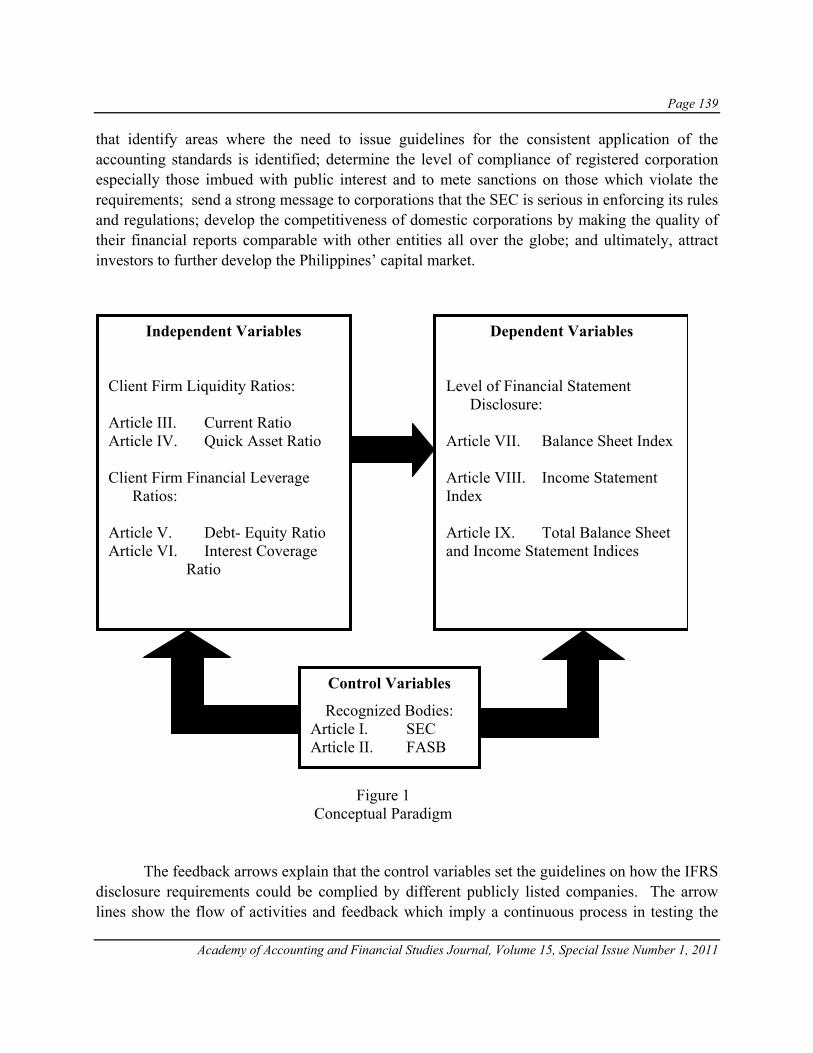
Page 139
Academy of Accounting and Financial Studies Journal, Volume 15, Special Issue Number 1, 2011
that identify areas where the need to issue guidelines for the consistent application of the accounting standards is identified; determine the level of compliance of registered corporation especially those imbued with public interest and to mete sanctions on those which violate the requirements; send a strong message to corporations that the SEC is serious in enforcing its rules and regulations; develop the competitiveness of domestic corporations by making the quality of their financial reports comparable with other entities all over the globe; and ultimately, attract investors to further develop the Philippines’ capital market.
The feedback arrows explain that the control variables set the guidelines on how the IFRS disclosure requirements could be complied by different publicly listed companies. The arrow lines show the flow of activities and feedback which imply a continuous process in testing the
Figure 1 Conceptual Paradigm
Control Variables
Recognized Bodies: Article I. SEC Article II. FASB
Independent Variables
Client Firm Liquidity Ratios:
Article III. Current Ratio Article IV. Quick Asset Ratio Client Firm Financial Leverage
Ratios:
Article V. Debt- Equity Ratio Article VI. Interest Coverage
Ratio
Dependent Variables
Level of Financial Statement
Disclosure:
Article VII. Balance Sheet Index
Article VIII. Income Statement Index Article IX. Total Balance Sheet and Income Statement Indices

Page 140
Academy of Accounting and Financial Studies Journal, Volume 15, Special Issue Number 1, 2011
relationship and effect of liquidity and financial leverage ratios with the degree of compliance with IFRS among publicly listed corporations in the Philippines.
STATEMENT OF THE PROBLEM Is there a significant relationship between liquidity and financial leverage ratios with International Financial Reporting Standard disclosure when the latter is expressed in terms of Balance Sheet and Income Statement indices? Does the degree of compliance with International Financial Reporting Standard disclosure as measured by Balance Sheet and Income Statement indices exert a significant effect on financial performance of Publicly Listed Corporations?
HYPOTHESES
Ho: There is no significant relationship between the liquidity and financial leverage ratios of publicly listed corporations (PLCs) in the Philippines and that of compliance with Internal Financial Reporting Standard disclosure in terms of Balance Sheet and Income Statement Indices.
Ho: The liquidity and financial leverage indicators of publicly listed corporations are
not significantly affected by International Reporting Standard disclosure index.
TREATMENT OF DATA Disclosure indices were constructed from 475 items of Balance Sheet disclosure checklist and 263 items of Income Statement disclosure checklist based on the 2007 compliance audit consistent with the International Financial Reporting Standard (IFRS) Report Checklist. A dichotomous scoring procedure was applied to each of the above items per publicly listed corporation by assigning a value of “1” if compliance is satisfactorily met and a value of “0” if not met. Thereafter, the scores for the Balance Sheet items are totaled and divided by total number of items. Likewise for Income Statement index. The resulting quotient is a relative measure of degree of compliance by a PLC.
STATISTICAL TREATMENT A multiple regression analysis was performed to test if liquidity and financial leverage indicators of publicly listed corporations are not significantly affected by International Reporting Standard disclosure index. The regression equations are as follows:

Page 141
Academy of Accounting and Financial Studies Journal, Volume 15, Special Issue Number 1, 2011
BS = ß0 + ß1CRInd i + ß2QRind i i + ß3DRInd i + ß4ICRind i i + e i IS = ß0 + ß1CRInd i + ß2QRind i i + ß3DRInd i + ß4ICRind i i + e i TBSIS = ß0 + ß1CRInd i + ß2QRind i i + ß3DRInd i + ß4ICRind i i + e i where: BS= balance sheet index of a firm; IS = income statement index of a firm; CRInd I = current ratio of a firm; QRInd 2 = quick ratio of a firm; DRInd I3= debt equity ratio of the firm; ICRInd 4 = interest coverage ratio; e 1 = Error term or disturbance term attributable to unknown factors. The statistical significance of the individual regression coefficients were tested using the Studentized residual or t-test.
t-ratio = regression coefficient standard error of coefficient
while the overall significance of each regression model was determined by calculating the corresponding coefficient of determination or R2 and its corresponding F-ratio, viz:
R2 = 1 - ∑e2
∑y2
where ∑e2 = squared deviations of estimates from actual observation ∑y2 = squared difference of actual data from its mean and
F-ratio = R2 / k – 1 (1 – R2) / n – k
where k = number of explanatory variables n = sample size If the computed F-ratio exceeds critical values at a specified level of significance, say 5 percent, and degrees of freedom, then the regression model is deemed statistically significantly different from zero. In other words, the explanatory variables, taken collectively, exert a significant effect on the dependent variable of choice. It is also a test of significance of the R2 which in turn measures the “goodness of fit” of the model.

Page 142
Academy of Accounting and Financial Studies Journal, Volume 15, Special Issue Number 1, 2011
MEASURES OF LIQUIDITY AND FINANCIAL LEVERAGE RATIOS Liquidity The term working capital is used to describe the current items of the balance sheet. Working capital includes current assets such as cash, accounts receivable, and inventory, and current liabilities such as accounts payable and other short term liabilities. Net working capital is defined as non-cash current operating assets minus non-debt current operating liabilities. Cash, short-term debt, and current portion of long-term debt are excluded from the net working capital calculation because they are related to financing and not to operations. Financial Leverage Ratios Any ratio used to calculate the financial leverage of a company to get an idea of the company's methods of financing or to measure its ability to meet financial obligations. There are several different ratios, but the main factors looked at include debt, equity, assets and interest expenses. A ratio used to measure a company's mix of operating costs, giving an idea of how changes in output will affect operating income. Fixed and variable costs are the two types of operating costs; depending on the company and the industry, the mix will differ. The following measures ratios of publicly listed corporations (PLCs) represent the independent variables of the regression models: The Current Ratio (or Working Capital) is the ratio of current assets to current liabilities. Working capital is a company's biggest safety net against financial disaster. Current Ratio = current assets / current liabilities
The Quick Ratio (or Acid Test) is considered more stringent than the Current Ratio. In this formula, inventories and paid expenses are removed from the current assets because they often can not be turned back into cash or liquidated quickly.
Quick Ratio = (cash + investments + receivables) / current liabilities The Debt Ratio is derived by subtracting the company's total assets from its total debt. Debt Ratio = total debt / total assets The Interest Coverage, the Times Interest Earned Ratio measures a company's ability to handle the interest
payments of long-term debt. Times Interest Earned Ratio = earnings before interest (EBIT) / interest charges (http://www.ehow.com/how_2364215_calculate-financial-ratios.html)
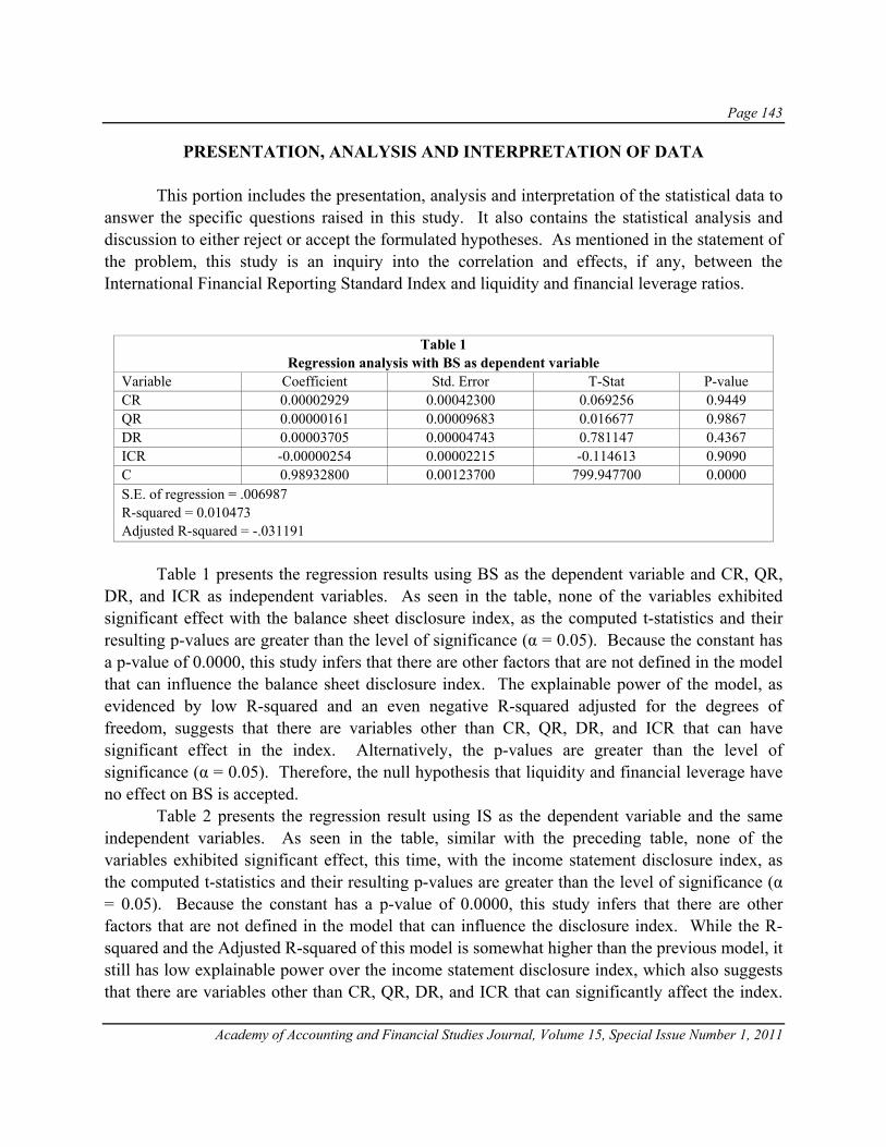
Page 143
Academy of Accounting and Financial Studies Journal, Volume 15, Special Issue Number 1, 2011
PRESENTATION, ANALYSIS AND INTERPRETATION OF DATA This portion includes the presentation, analysis and interpretation of the statistical data to answer the specific questions raised in this study. It also contains the statistical analysis and discussion to either reject or accept the formulated hypotheses. As mentioned in the statement of the problem, this study is an inquiry into the correlation and effects, if any, between the International Financial Reporting Standard Index and liquidity and financial leverage ratios.
Table 1 presents the regression results using BS as the dependent variable and CR, QR, DR, and ICR as independent variables. As seen in the table, none of the variables exhibited significant effect with the balance sheet disclosure index, as the computed t-statistics and their resulting p-values are greater than the level of significance (α = 0.05). Because the constant has a p-value of 0.0000, this study infers that there are other factors that are not defined in the model that can influence the balance sheet disclosure index. The explainable power of the model, as evidenced by low R-squared and an even negative R-squared adjusted for the degrees of freedom, suggests that there are variables other than CR, QR, DR, and ICR that can have significant effect in the index. Alternatively, the p-values are greater than the level of significance (α = 0.05). Therefore, the null hypothesis that liquidity and financial leverage have no effect on BS is accepted. Table 2 presents the regression result using IS as the dependent variable and the same independent variables. As seen in the table, similar with the preceding table, none of the variables exhibited significant effect, this time, with the income statement disclosure index, as the computed t-statistics and their resulting p-values are greater than the level of significance (α = 0.05). Because the constant has a p-value of 0.0000, this study infers that there are other factors that are not defined in the model that can influence the disclosure index. While the R-squared and the Adjusted R-squared of this model is somewhat higher than the previous model, it still has low explainable power over the income statement disclosure index, which also suggests that there are variables other than CR, QR, DR, and ICR that can significantly affect the index.
Table 1 Regression analysis with BS as dependent variable
Variable Coefficient Std. Error T-Stat P-value CR 0.00002929 0.00042300 0.069256 0.9449 QR 0.00000161 0.00009683 0.016677 0.9867 DR 0.00003705 0.00004743 0.781147 0.4367 ICR -0.00000254 0.00002215 -0.114613 0.9090 C 0.98932800 0.00123700 799.947700 0.0000 S.E. of regression = .006987 R-squared = 0.010473 Adjusted R-squared = -.031191

Page 144
Academy of Accounting and Financial Studies Journal, Volume 15, Special Issue Number 1, 2011
Alternatively, the p-values are greater than the level of significance (α = 0.05). Therefore, the null hypothesis that liquidity and financial leverage have no effect on IS is accepted.
Table 2 Regression analysis with IS as dependent variable
Variable Coefficient Std. Error T-Stat P-value TQ 0.00030949 0.00027110 1.141596 0.2565 ROA 0.00000399 0.00006207 0.064289 0.9489 ROE 0.00002925 0.00003040 0.962080 0.3385 EPS -0.00002514 0.00001420 -1.771194 0.0797 C 0.99385300 0.00079300 1253.691000 0.0000 S.E. of regression = 0.004478 R-squared = 0.059896 Adjusted R-squared = 0.020313
Table 3 presents the regression results using the combined indices of balance sheet and income statement disclosures as the dependent variable and the independent variables used in prior tables. From this presentation, the study identified none of the variables that is significantly related to the variables, except for the constant, whose figures indicate that there are other variables than CR, QR, DR, and ICR that will exhibit significant influence with the indices used. Alternatively, the p-values are greater than the level of significance (α = 0.05). Therefore, the null hypotheses that liquidity and financial leverage have no effect on Total BS and IS, is accepted.
Table 3 Regression analysis with TBSIS as dependent variable
Variable Coefficient Std. Error t-Statistic Prob. TQ 0.00012915 0.00031359 0.411838 0.6814 ROA 0.00000246 0.00007180 0.034284 0.9727 ROE 0.00003427 0.00003516 0.974517 0.3323 EPS -0.00001059 0.00001642 -0.645186 0.5204 C 0.99094000 0.00091700 1080.681 0.0000 S.E. of regression = 0.00518 R-squared = .021638 Adjusted R-squared = -0.019556
Table 4 shows the results of the analysis of variance of the model with the balance sheet disclosure index as the dependent variable. With a p-value of .9082 which is higher than the level

Page 145
Academy of Accounting and Financial Studies Journal, Volume 15, Special Issue Number 1, 2011
of significance, this study reveals the insignificance of the model to influence the disclosure index in the balance sheet. This can be explained by the non-significance of CR, QR, DR, and ICR to influence such disclosures.
Table 4 Analysis of variance of the model with BS as dependent variable
Source SS df MS F p-value Regression 0.00004908 4 0.00001227 0.25 .9082 Residual 0.00463741 95 0.00004881 Total 0.00468649 99
Table 5 shows the results of the analysis of variance of the model with the income statement disclosure index as the dependent variable. With a p-value of .2045 which is higher than the level of significance, this study identifies, similar in the previous model, the insignificance of the entire model to influence the income statement disclosure index. This can be explained by the non-significance of CR, QR, DR, and ICR to influence IFRS disclosures.
Table 5 Analysis of variance of the model with IS as dependent variable
Source SS df MS F p-value Regression 0.00012140 4 0.00003035 1.51 .2045 Residual 0.00190538 95 0.00002006 Total 0.00202678 99
Table 6 shows the results of the analysis of variance of the model with the combined indices of the balance sheet and income statement as the dependent variable. With an F-statistics of 0.53, the model’s p-value equals 0.7174 which is higher than the level of significance. Thus, this study finds and insignificant relationship between the variables of interest and the disclosure index.
Table 6 Analysis of variance of the model with TBSIS as dependent variable
Source SS df MS F p-value Regression 0.00005638 4 0.00001410 0.53 .7174 Residual 0.00254928 95 0.00002683 Total 0.00260567 99

Page 146
Academy of Accounting and Financial Studies Journal, Volume 15, Special Issue Number 1, 2011
TESTING FOR PLAUSIBILITY AND ROBUSTNESS This section highlights the test that were carried out to determine the plausibility and robustness of the model used or make sure that the model does not violate the fundamental assumptions of ordinary least squares which is crucial to the precision of the results it will generate. The OLS assumptions known as multicollinearity, heteroskedasticity, and autocorrelation.
TESTING FOR MULTICOLLINEARITY To determine whether the proposed model has committed the violation of multicollinearity or the presence of a linear relationship among the variables, this study performed the Variance Inflation Factor (VIF). As a rule of thumb, the VIF must not exceed 10, otherwise, it is an indication that multicollinearity exists.
Table 7 Variance inflation factors (VIF) of the variables
Variable Coefficient CR 1.018 QR 1.601 DR 1.600 ICR 1.009 C Mean VIF 1.307
To test whether the variables have complied or have not complied to the assumptions of the ordinary least squares regression model, this study applied the different tests of multicollinearity, heteroskedasticity, and autocorrelation. Table 7 presents the variance inflation factors (VIF) of the variables. The same figures appear on the regression analyses despite the difference in the independent variables, as this test identifies the presence or absence of a linear relationship between the variables. This study noted that the coefficients and the mean VIF are less than the critical value of 10. As such, there is an absence of a linear relationship between the variables.
TESTING FOR HETEROSKEDASTICITY To test the presence or absence of any violation that the model might have committed, the model underwent the White’s Test, using the EVIEWS software, for Heteroskedasticity which means that the error of each observation must come form the same probability distribution.

Page 147
Academy of Accounting and Financial Studies Journal, Volume 15, Special Issue Number 1, 2011
One way of proving the non-existence of heteroskedasticity was by comparing the p-values and the level of significance (α). If the p-value is greater than α, then the probability of incorrect rejection of the null hypothesis of no heteroskedasticity is greater than its level of significance; then indicating the absence of non-constant variation in the residual terms.
Table 8 Summary results of the White’s Heteroskedasticity test for all models
Variable Df White's Test Statistic > or < Critical χ2 P-value > or < Α
BS 14 0.550729 < 23.6847913 1.000000 > 0.05 IS 14 13.27611 < 23.6847913 0.504907 > 0.05 TBSIS 14 0.699166 < 23.6847913 1.00000 > 0.05
To test the presence or absence of constant variances among the variables, this study performed the White’s Test of heteroskedasticity. Table 8 presents the summary results. As this study utilized the cross terms method of the test, this study noted that the White’s Test statistic is less than the critical chi-square values given the degrees of freedom. Moreover, the p-values computed are greater than the level of significance that indicates the absence of non-constant variances among the variables. Thus, this study finds that there is no heteroskedasticity in the models.
TESTING FOR AUTOCORRELATION The Durbin–Watson statistics is a test statistic used to detect the presence of autocorrelation in the residuals from a regression analysis. It is named after James Durbin and Geoffrey Watson. Autocorrelation is commonly seen or is endemic in time-series analysis or the presence of spatial correlation across the order of observations in a cross-sectional econometric model, it is still important to establish that autocorrelation is not present in the model to enhance the integrity of the conclusion drawn from it. This study used the Run’s test to verify the true state of autocorrelation in the IFRS index model. Using the MEGASTAT software, the expected value of residuals [ E ( resid)] and the variance of residuals (σr
2) is computed as
E(resid) = 2T1T2 + 1 T
σr2 = 2T1T2 (2T1T2 – T)
T2 (T – 1)

Page 148
Academy of Accounting and Financial Studies Journal, Volume 15, Special Issue Number 1, 2011
where: T1 = number of positive residuals T2 = number of negative residuals T = number of observations; and σr
2 = variance of residuals. Incidentally, σr refers to the standard deviation of residuals computed as the square root of the variance.
Substituting the formula, this method obtained the figures as presented on Table 9 that will be needed for the Run’s test.
Table 9 Summary results of the Autocorrelation for all models
Item Designation Values BS IS TBSIS
T1 Number of positive residuals 63 56 63 T2 Number of negative residuals 37 44 37 T Number of observations 100 100 100 E (resid) Expected value of residuals 47.62 50.28 47.62 σr
2 Variance of residuals 21.43578 24.03271 21.43578 σr Standard deviation of residuals 4.62988 4.902317 4.62988 Min Minimum Runs 38.5454 40.67 38.5454 Max Maximum Runs 56.6946 59.8885 56.6946 Runs Observed Runs 44 45 45
To test the presence or absence of serial correlation among the observations, this study performed the Run’s test of autocorrelation. Table 9 presents the summary results. The researcher identified the number of changes in the residual and treated such changes as runs. Under this test, the model commits the violation of autocorrelation when the number of runs fell above the maximum or below the minimum runs as identified by the allowable range provided by the standard normal distribution. Using the computations, it can be observed that the number of runs for all models fall within the maximum and minimum runs; thus providing strong evidence that there is no autocorrelation in our models.
CONCLUSIONS Based on the above findings in this study, conclusions have been drawn. They are discussed as follows: Using multiple regression analysis, the author regressed each of balance sheet index, income statement index and total of income statement – balance sheet indices, against liquidity
Page 149
Academy of Accounting and Financial Studies Journal, Volume 15, Special Issue Number 1, 2011
ratios and financial leverage ratios such as current ratio, quick ratio, debt ratio and interest coverage ratio. None of the indices exert a significant effect on the financial variables cited based on the computed t-statistics whose p-values are greater than the level of significance (α = 0.05). Therefore, the null hypothesis, that liquidity and financial leverage have no effect on IFRS when the latter is expressed in terms of Balance Sheet and Income Statement indices, is accepted. The OLS assumptions known as multicollinearity, heteroskedasticity, and autocorrelation were utilized. This study noted that the coefficients and the mean VIF are less than the critical value of 10. As such, there is an absence of a linear relationship between the variables. As this study utilized the cross terms method of the test, this study noted that the White’s Test statistic is less than the critical chi-square values given the degrees of freedom. Moreover, the p-values computed are greater than the level of significance that indicates the absence of non-constant variances among the variables. Thus, this study finds that there is no heteroskedasticity in the models. The researcher identified the number of changes in the residual and treated such changes as runs. Under this test, the model commits the violation of autocorrelation when the number of runs fell above the maximum or below the minimum runs as identified by the allowable range provided by the standard normal distribution. Using the computations, it can be observed that the number of runs for all models fall within the maximum and minimum runs; thus providing strong evidence that there is no autocorrelation in our models.
REFERENCES Bhat, G., O.-K. Hope and T. Kang (2006), “Does corporate governance transparency affect the accuracy of analyst
forecasts?”, Accounting and Finance,(46)5, 715-732. Cadbury Code, The (1992), Report of the Committee on the Financial Aspects of Corporate Governance: The Code
of Best Practices, December, Gee Professional Publishing, London. Debrency, R. and G.L. Gray (2001). Financial reporting on the Internet and the external audit (Abstract). European
Accounting Review, 8:2, 335-350. Dye, R., and S. Sunder (2001). Why Not Allow FASB and IASB Standards to Compete in the U.S.? Accounting
Horizons 15, 257-272. Fama, E. F. (1980). Agency problem and the theory of the firm. Journal of political economy, 88, 288-308. Farrar J. and B. Hannigan (1998). Farrar’s Company Law, (4th Edition), Butterworths, London. Jensen, M. C. (1983). Separation of ownership and control. Journal of law and economics, 26, 301-325.

Page 150
Academy of Accounting and Financial Studies Journal, Volume 15, Special Issue Number 1, 2011
Kusumawati, N. (2006). Profitability and corporate governance disclosure: an Indonesian study. Simposium Nasional Akuntansi 9 Padang.
Lee, H., V. Mande, and R. Ortman (2004). The effect of audit committee and board of director independence on
auditor resignation. Auditing: A journal of practice and theory, 23(2)., 131-146. Leuz, Christian and Peter Wysocki (2008). Economic Consequences of Financial Reporting and Disclosure
Regulation: A Review and Suggestions for Future Research. Retrieved Jan 5, 2010, from http://ssrn.com/abstract=1105398
Richardson, V. (2000). Information asymmetry and earnings management: Some evidence. Review of quantitative
finance and accounting, 15, 325-347. Roberts J. (2004). Agency Theory Ethics and Corporate Governance, The Judge Institute of Management
University of Cambridge.