1D-LDA vs. 2D-LDA: When is vector-based linear discriminant ...

Pattern Recognition 41 (2008) 2156–2172www.elsevier.com/locate/pr

1D-LDA vs. 2D-LDA: When is vector-based linear discriminant analysisbetter than matrix-based?

Wei-Shi Zhenga,c, J.H. Laib,c,∗, Stan Z. Lid

aSchool of Mathematics and Computational Science, Sun Yat-sen University, Guangzhou, PR ChinabDepartment of Electronics and Communication Engineering, School of Information Science and Technology, Sun Yat-sen University, Guangzhou, PR China

cGuangdong Province Key Laboratory of Information Security, PR ChinadCenter for Biometrics and Security Research and National Laboratory of Pattern Recognition, Institute of Automation, Chinese Academy of Sciences,

Beijing, PR China

Received 18 August 2006; received in revised form 27 November 2007; accepted 29 November 2007

Abstract

Recent advances have shown that algorithms with (2D) matrix-based representation perform better than the traditional (1D) vector-basedones. In particular, 2D-LDA has been widely reported to outperform 1D-LDA. However, would the matrix-based linear discriminant analysis bealways superior and when would 1D-LDA be better? In this paper, we investigate into these questions and have a comprehensive comparisonbetween 1D-LDA and 2D-LDA in theory and in experiments. We analyze the heteroscedastic problem in 2D-LDA and formulate mathematicalequalities to explore the relationship between 1D-LDA and 2D-LDA; then we point out potential problems in 2D-LDA. It is shown that 2D-LDA has eliminated the information contained in the covariance information between different local geometric structures, such as the rowsor the columns, which is useful for discriminant feature extraction, whereas 1D-LDA could preserve such information. Interestingly, this newfinding indicates that 1D-LDA is able to gain higher Fisher score than 2D-LDA in some extreme case. Furthermore, sufficient conditions onwhich 2D-LDA would be Bayes optimal for two-class classification problem are derived and comparison with 1D-LDA in this aspect is alsoanalyzed. This could help understand how 2D-LDA is expected to achieve at its best, further discover its relationship with 1D-LDA, and wellsupport other findings. After the theoretical analysis, comprehensive experimental results are reported by fairly and extensively comparing1D-LDA with 2D-LDA. In contrast to the existing view that some 2D-LDA based algorithms would perform better than 1D-LDA when thenumber of training samples for each class is small or when the number of discriminant features used is small, we show that it is not alwaystrue and show that some standard 1D-LDA based algorithms could perform better in those cases on some challenging data sets.� 2007 Elsevier Ltd. All rights reserved.

Keywords: Fisher’s linear discriminant analysis (LDA); Matrix-based representation; Vector-based representation; Pattern recognition

1. Introduction

Over the last two decades, many subspace algorithms havebeen developed for feature extraction. Among them are prin-cipal component analysis (PCA) [1–4], (Fisher’s) linear dis-criminant analysis (LDA) [4–8], independent component anal-ysis (ICA) [9–12], non-negative matrix factorization (NMF)

∗ Corresponding author. Department of Electronics and CommunicationEngineering, School of Information Science and Technology, Sun Yat-senUniversity, Guangzhou, PR China. Tel.: +86 020 84035440.

E-mail addresses: [email protected] (W.-S. Zheng),[email protected] (J.H. Lai), [email protected] (S.Z. Li).

0031-3203/$30.00 � 2007 Elsevier Ltd. All rights reserved.doi:10.1016/j.patcog.2007.11.025

[13–15], locality preserving projection [16] and Bayesian prob-abilistic subspace [17,18], etc.

Most well-known subspace methods require the input pat-terns to be shaped in vector form. Recently there are effortsseeking to extract features directly without any vectorizationwork on image samples, i.e., the representation of an im-age sample is retained in matrix form. Based on this idea,some well-known algorithms are developed, including two-dimensional principal component analysis (2D-PCA) [19,20]and two-dimensional linear discriminant analysis (2D-LDA)[21–23].

2D-PCA was first proposed by Yang et al. [19,20], anda generalized work has been subsequently described in [24]

http://www.elsevier.com/locate/pr

mailto:[email protected]



W.-S. Zheng et al. / Pattern Recognition 41 (2008) 2156–2172 2157

called bilateral-projection-based 2DPCA (B2DPCA). Ye thenproposed the generalized low rank approximations of matrices(GLRAM) [25] as a further development of 2D-PCA. Recentlya modification on 2D-PCA was proposed in Ref. [26] and itcould be treated as implementing 2D-PCA after rearrangementof the entries of an image matrix.

For supervised learning, 2D-LDA has also been developedrecently. Xiong et al. [22] and Li et al. [21] extended one-dimensional LDA (1D-LDA), a vector-based scheme, to 2D-LDA. In contrast to [21,22] which only do transform on oneside of the image matrix, i.e., either left side or right side, somemethods have been proposed for extraction of the discrimina-tive transforms on both sides of the image matrix. Yang et al.[27] proposed to do the IMLDA (uncorrelated image matrix-based LDA) twice, i.e., IMLDA is first implemented to find theoptimal discriminant projection on the right side of the matrixand then to find another optimal discriminant projection on theleft side. Similarly, Kong et al. [28] proposed to first extract the2D-LDA discriminative projections on both sides of the imagematrix independently and then combine them by some process-ing. Different from them, Ye et al. proposed an iterative schemeto extract the transforms on both sides [23] simultaneously.Recently, some other modifications on 2D-LDA [29–31] areproposed. Especially, in Ref. [30], similar to Fisherface [8], 2D-LDA is processed after the implementation of 2D-PCA. Thoughsuch rapid development appeared in the last two years; however,Liu et al. [32] actually had suggested a 2D image matrix-based(Fisher’s) linear discriminant technique which performed LDAdirectly on image matrices in 1993. In nature, the idea behindis to construct the covariance matrix, including total-class scat-ter matrix, within-class scatter matrix and between-class scattermatrix, by just using the original image samples representedin matrix form. Moreover, some recent studies [24,28,33,34]have realized that two-dimensional matrix-based algorithms arespecial blocked-based methods such as column-based or row-based LDA\PCA in essence.

2D-LDA is attractive since it is efficient in computation andalways avoids the “small sample size problem” [8,35–38] thatthe within-class scatter matrix is always singular in 1D-LDAwhen the training sample size is (much) smaller than the dimen-sionality of the data. Recently, the 2D-LDA based algorithmshave been experimentally reported superior to some standard1D-LDA based algorithms, such as Fisherface [8], on somelimited data sets.

However, one may ask: “Could 2D-LDA always perform thebest?” “Why would it be better sometimes?” “Is there any draw-back in 2D-LDA?” “What is the intrinsic relationship between1D-LDA and 2D-LDA?” “1D-LDA is Bayes optimal for two-class classification under some sufficient conditions, and thenwhat is the situation for 2D-LDA? What are the differences be-tween 1D-LDA and 2D-LDA under their sufficient conditionsbeing Bayes optimal?” After all, “When is 1D-LDA better than2D-LDA?”

We do investigation into these questions and present an ex-tensive analysis between 1D-LDA and 2D-LDA in theory andin experiments. This is, to the best of our knowledge, the firstof such attempt with comprehensive study. The contributions

of this paper are summarized as follows:

(1) Extensive theoretical comparisons between 1D-LDA and2D-LDA are presented, and we have the following findings:(a) From the statistical point of view, 2D-LDA would also

be confronted with the “Heteroscedastic Problem” andthe problem would be more serious for 2D-LDA thanthe one for 1D-LDA.

(b) Mathematical equalities are formulated to explore therelationship between 1D-LDA and 2D-LDA. It gives anovel way to show that 2D-LDA loses the covarianceinformation among different local geometry structuresin the image such as rows or columns, while 1D-LDAcould preserve those relations for feature extraction. Itthen breaks the appearance view that 2D-LDA is ableto utilize the global geometry structure of an image.Interestingly, we further find that 1D-LDA is able toachieve higher Fisher score than 2D-LDA in some ex-treme case as shown in the paper.

(c) The sufficient conditions when 2D-LDA is Bayes opti-mal for two-class classification problem are given andproved. They could help give an interpretation what2D-LDA is expected ideally. Moreover further discus-sions between 1D-LDA and 2D-LDA are presentedwhen those sufficient conditions are satisfied or not.

(2) Extensive experiments are conducted to compare 1D-LDAwith 2D-LDA. The experimental results break the existingviews and indeed show that 2D-LDA would not always besuperior to 1D-LDA when the number of training samplesfor each class is small or when the number of discriminantfeatures used is small.

Though this paper focuses on (Fisher’s) LDA; however, theanalysis could be useful for other similar algorithms. The re-mainder of this paper is outlined as follows. In Section 2, a briefreview of 1D-LDA and 2D-LDA is given. In Section 3, the-oretical analysis between 1D-LDA and 2D-LDA is presented.In Section 4, extensive experiments are conducted. Finally, wehave a summarization in Section 5.

2. Reviews

2.1. Notations

Suppose {(x11, X1

1, C1), . . . , (x1N1

, X1N1

, C1), . . . , (xL1 , XL

1 ,

CL), . . . , (xLNL

, XLNL

, CL)} are image samples from L classes.

The n-dimensional vector xki ∈ Rn is the ith sample of the kth

class Ck and Xki ∈ Rrow×col is its corresponding row × col

image matrix, where i = 1, . . . , Nk and Nk is the number oftraining samples of class Ck . Let N = ∑L

j=1Nj be the total

sample size. Define uk = 1Nk

∑Nk

i=1 xki as the mean vector of

samples of class Ck and Uk = 1Nk

∑Nk

i=1 Xki as its corresponding

mean matrix. Let u =∑Lk=1

Nk

Nuk be the mean vector of all

samples and U=∑Lk=1

Nk

NUkbe its corresponding mean matrix.

2158 W.-S. Zheng et al. / Pattern Recognition 41 (2008) 2156–2172

2.2. 1D-LDA (one-dimensional LDA)

1D-LDA aims to find the discriminative vector wopt such that

wopt = arg maxw

wTSbwwTSww

, (1)

where Sb=∑Lk=1

Nk

N(uk−u)(uk−u)T, Sw= 1

N

∑Lk=1∑Nk

i=1 (xki −

uk)(xki −uk)

T=∑Lk=1

Nk

NSk

w, Skw= 1

Nk

∑Nk

i=1 (xki −uk)(xk

i −uk)T

are between-class scatter matrix, within-class scatter matrixand within-class scatter matrix of class Ck , respectively. Inpractice, due to the curse of high dimensionality, Sw is alwayssingular. So far, some well-known standard variations of 1D-LDA have been developed to overcome this problem, such asFisherface [8] and its further developments [40,41], NullspaceLDA [35–37], direct LDA [42], LDA/QR [38,43] and regular-ized LDA [5,44–47], etc. Thereof, regularized LDA is alwaysimplemented as follows:

wr-opt = arg maxw

wTSbwwT(Sw + � I)w

, � > 0. (2)

Other efforts are also made for obtaining more discriminativeand robust 1D-LDA algorithms in the small sample size case,such as constraint-based LDA algorithm [48,49], weight-basedLDA algorithm [50], mixture model-based LDA [51], locallyLDA [52] and oriented LDA [53], etc.

2.3. 2D-LDA (two-dimensional LDA)

2D-LDA directly performs discriminant feature analysis onan image matrix rather than on a vector. 2D-LDA tries to findthe optimal vector w2d

opt such that

w2dopt = arg max

w2d

w2dTS2d

b w2d

w2dTS2dw w2d

, (3)

where S2db = ∑L

k=1Nk

N(Uk − U)(Uk − U)T and S2d

w =1N

∑Lk=1∑Nk

i=1 (Xki − Uk)(Xk

i − Uk)T are between-class scatter

matrix and within-class scatter matrix, respectively. An alter-native approach of 2D-LDA could be driven by the followingcriterion:

w̃2dopt = arg max

w̃2d

w̃2dTS̃2d

b w̃2d

w̃2dTS̃2dw w̃2d

, (4)

where S̃2db = ∑L

k=1Nk

N(Uk − U)T(Uk − U) and S̃2d

w =1N

∑Lk=1∑Nk

i=1 (Xki − Uk)

T(Xki − Uk).

Equality (Criterion) (3) or (4) is called the unilateral 2D-LDA [28]. As aforementioned, a generalization of 2D-LDAcalled the bilateral 2D-LDA (B-2D-LDA) [23,28] finds a pairdiscriminant vectors (w2d

l-opt , w2dr-opt ) satisfying:

(w2dl-opt , w2d

r-opt ) = arg max(w2d

l ,w2dr )∑L

k=1Nk

Nw2d

l

T(Uk−U)w2d

r w2dr

T(Uk−U)Tw2d

l

1N

∑Lk=1∑Nk

i=1 w2dl

T(Xk

i −Uk)w2dr w2d

rT(Xk

i −Uk)Tw2d

l

. (5)

3. 1D-LDA vs. 2D-LDA: theoretical analysis

In this part, to compare with 1D-LDA, we first mainly focuson 2D-LDA in terms of equality (3). It does not mean thecomparison would lose the generality. It is because equality (4)would become equality (3) if the input matrices are transposedfirst, and also so far it is hard to obtain a closed form solutionbut a practical solution [23,28,54] is popular and always foundfor equality (5). Analysis will be extended to the variations of2D-LDA in terms of equalities (4)–(5) in Section 3.4.

Without loss of generality, define Xki = [Xk

i (1), Xki (2), . . . ,

Xki (col)] ∈ Rrow×col and its corresponding vector form xk

i =[Xk

i (1)T, Xki (2)T, . . . , Xk

i (col)T]T, where Xki (j) ∈ Rrow×1 is

the j th column of matrix Xki . We then have

Uk = [Uk(1), . . . , Uk(col)]

=⎡⎣ 1

Nk

Nk∑i=1

Xki (1), . . . ,

1

Nk

Nk∑i=1

Xki (col)

⎤⎦ ,

U = [U(1), . . . , U(col)]

=[

L∑k=1

Nk

NUk(1), . . . ,

L∑k=1

Nk

NUk(col)

],

uk = [Uk(1)T, . . . , Uk(col)T]T,

u = [U(1)T, . . . , U(col)T]T.

As indicated in Refs. [28,33], it is easy to verify the following:

S2db =

L∑k=1

Nk

N

col∑j=1

(Uk(j) − U(j))(Uk(j) − U(j))T

= S2db,1 + · · · + S2d

b,col , (6)

S2dw = 1

N

L∑k=1

Nk∑i=1

col∑j=1

(Xki (j) − Uk(j))(Xk

i (j) − Uk(j))T

= S2dw,1 + · · · + S2d

w,col , (7)

where

S2db,j =

L∑k=1

Nk

N(Uk(j) − U(j))(Uk(j) − U(j))T,

j = 1, . . . , col,

S2dw,j = 1

N

L∑k=1

Nk∑i=1


i (j) − Uk(j))T,

j = 1, . . . , col.

3.1. Heteroscedastic problem

First the 2D-LDA criterion in terms of equality (3) could beequivalently written as

w2dopt = arg max

w2d

w2dT{

1col

∑colj=1 S2d

b,j

}w2d

w2dT{

1col

∑colj=1 S2d

w,j

}w2d

.


It can be found that the between-class information of 2D-LDAin terms of equality (3) is modeled by averaging all between-class scatter matrices S2d

b,j with respect to different column in-dexes and models the within-class information similarly by av-eraging all S2d

w,j . From the statistical point of view, both S2db

and S2dw are “plug-in” estimates according to equalities (6)–(7).

However, if columns with different indexes of images are het-eroscedastic in essence, i.e., S2d

b,j �= S2db,i , ∀i �= j or S2d

w,j �=S2d

w,i , ∀i �= j , then those “plug-in” estimates S2db and S2d

w would

be inappropriate if the differences between S2db,j or the differ-

ences between S2dw,j are significantly large. In such case the

heteroscedastic problem [39] has to be addressed. We note that1D-LDA would also be confronted with the heteroscedasticproblem when the covariance matrices of different classes, i.e.,Sk

w, k = 1, . . . , L, are not equal [39], and it breaks the assump-tion of LDA that within-class covariance matrices of all classesare equal. However, the problem for 2D-LDA is different fromthe one for 1D-LDA in the following aspects. It is observedthat samples learned by 2D-LDA in terms of equality (3) areactually the columns of images according to equalities (6)–(7),while columns are always obviously different if they are notcoherent. Hence, on one hand, for estimation of within-classscatter information, columns with different indexes of imageswithin the same class could be heteroscedastic (i.e., S2d

w,j arenot equal), even if the image samples in vector form are notheteroscedastic (i.e., Sk

w are equal). On the other hand, the het-eroscedastic problem in 1D-LDA is mainly due to the unequalwithin-class covariance matrices of different classes, but sucha problem could additionally happen to S2d

b in 2D-LDA for es-timation of between-class scatter information, because it is for-mulated by averaging all S2d

b,j . Therefore, it would be expectedthat the heteroscedastic problem in 2D-LDA could be more se-rious than that in 1D-LDA. However, such a seriously potentialproblem in 2D-LDA has not been pointed out before.

3.2. Relationship between 1D-LDA and 2D-LDA

Let w=[�wT

1 , . . . ,�w

T

col]T be any n-dimensional vector, where�wi ∈ Rrow×1. To explore the relationship between 1D-LDAand 2D-LDA, we first have the following lemma, and its proofcan be found in Appendix A.

Lemma 1. If�w1, . . . ,

�wcol ∈ Rrow×1 are imposed to be

equivalent, i.e.,

w2d = �w1 = · · · = �

wcol ∈ Rrow×1, (8)

then the following relations are valid:

w̃TSbw̃ = w2dTS2d

b w2d + w2dT

⎧⎨⎩

L∑k=1

Nk

N

col∑j=1,h=1,j �=h

(Uk(j)

−U(j))(Uk(h) − U(h))T

⎫⎬⎭w2d , (9)

w̃TSww̃ = w2dTS2dw w2d + w2dT

⎧⎪⎨⎪⎩

1

N

L∑k=1

Nk∑i=1


(Xki (j)

−Uk(j))(Xki (h) − Uk(h))T

⎫⎪⎬⎪⎭w2d , (10)

where

w̃ =⎡⎣w2dT

, . . . , w2dT︸︷︷︸col

⎤⎦T

. (11)

2D-LDA is apparently indicated to preserve global geomet-ric information of image since it directly lies on samples rep-resented in image matrix form. However, the above lemma re-veals that unlike 1D-LDA, it may lose the covariance infor-mation among different local geometry structures, such as thecolumns here. This is because in equalities (9) and (10), sum-mation of the covariance information of data after a 2D-LDAtransform and the eliminated covariance information by 2D-LDA between different local geometry structures is just the co-variance information of data after a special 1D-LDA transform,

where w2dTS2d

b w2d is the between-class covariance informa-

tion and w2dTS2d

w w2d is the within-class covariance informa-tion induced by the 2D-LDA transform w2d . Hence 2D-LDAdoes not completely utilize global geometric information of animage. Though w̃ is a special row · col( = n) dimensional vec-tor; however, equalities (9)–(10) suggest 1D-LDA could pre-serve those information.

Although some recent studies [28,33] have indicated that2D-LDA is a special block-based algorithm; however, the re-lationship between 1D-LDA and 2D-LDA has not been furtherexplored theoretically as shown in equalities (9) and (10) be-fore. Based on them, we here provide a new way to reveal thatthose part-based local geometric structures are considered sep-arately and show the covariance information between them isnot taken into account by 2D-LDA in theory.

Furthermore, the relationship formulated by Lemma 1 couldin fact provide a more in-depth insight view. The followingtheorem then tells such an interesting issue.

Theorem 1. 1 D-LDA can have higher Fisher score than 2D-LDA if the following cases are valid:

L∑k=1

Nk

N


(Uk(j) − U(j))(Uk(h) − U(h))T = 0,

(12)1

N

L∑k=1

Nk∑i=1



i (h)

− Uk(h))T = 0. (13)

Proof. In such a case, the following relations hold:

w̃TSbw̃ = w2dTS2d

b w2d , (14)

w̃TSww̃ = w2dTS2d

w w2d . (15)


Since w̃ is just a special n-dimensional vector, hence it is validthat:

maxw2d∈Rrow

w2dTS2d

b w2d

w2dTS2dw w2d

� maxw∈Rn

wTSbwwTSww

. (16)

That is, 1D-LDA can obtain higher Fisher score than2D-LDA. �

One situation when equalities (12) and (13) are valid is thecase that columns with different indexes of image matrices arestatistically independent. A further interpretation of equality(16) in such case could be provided from another point of viewin next section.

3.3. 2D-LDA: a Bayes optimal feature extractor undersufficient conditions

It is known that for two-class classification problem 1D-LDAwill be Bayes optimal if data are normally distributed with equalcovariance matrices within each class [4,5]. Then what is thesituation for 2D-LDA? The analysis here attempts to seek thesufficient conditions when 2D-LDA would be Bayes optimalfor two-class classification. Finally, the differences between1D-LDA and 2D-LDA will be discussed when those sufficientconditions are satisfied or not.

Suppose X = [X(1), . . . , X(col)] is a random Rrow×col ma-trix, where X(j) ∈ Rrow, j=1, . . . , col. Let p(X) and p(X(j))

be the probability density functions of X and X(j), respec-tively, and let p(X|Ck)and p(X(j)|Ck) be the class-conditionalprobability density functions of class Ck . Then it is valid that

p(X) = p(X(1), . . . , X(col)),

p(X|Ck) = p(X(1), . . . , X(col)|Ck).

If X(1), . . . , X(col) are independent, we then have

p(X) =col∏j=1

p(X(j)), p(X|Ck) =col∏j=1

p(X(j)|Ck). (17)

Given two classes C1 and C2, to classify X using Bayesiandecision principle, it is said X ∈ C1 if and only ifp(C1|X) > p(C2|X) else X ∈ C2. Note that P(Ck|X) =p(X|Ck)P (Ck)

p(X), where P(Ck) is the prior probability of class Ck .

If X(1), . . . , X(col) are assumed to be independent,1 then

P(Ck|X) =col∏j=1

p(X(j)|Ck)

p(X(j))P (Ck), (18)

log(P (Ck|X)) =col∑j=1

{log(p(X(j)|Ck)) − log(p(X(j)))}

+ log(P (Ck)). (19)

1This condition could be strict and a discussion will be given at the endof this section.

If all the j th columns X(j) of the kth class Ck are normallydistributed with mean Mk(j) and covariance matrix �j

k , i.e.,

p(X(j)|Ck) = (2�)−row/2|�jk |−1/2 exp{− 1

2 (X(j)

− Mk(j))T(�jk )

−1(X(j) − Mk(j))},

log(p(X(j)|Ck)) = − row

2log 2� − 1

2 log |�jk | − 1

2 (X(j)

− Mk(j))T(�jk )

−1(X(j) − Mk(j)) (20)

then the Bayes classifier function gk(X) can be formulated as

gk(X) = log(P (Ck|X))

=col∑j=1

{− row

2log 2� − 1

2log |�j

k | − 1

2(X(j)

−Mk(j))T(�jk )

−1(X(j) − Mk(j)) − log(p(X(j)))

}+ log(P (Ck)). (21)

In practice, utilizing the maximum likelihood principle, Mk(j)

and �jk could be estimated by

M̂k(j) = (Nk)−1

Nk∑i=1

Xki (j) = Uk(j), (22)

�̂jk = (Nk)

−1Nk∑i=1


i (j) − Uk(j))T, (23)

where Xki (j) is the j th column of the ith sample matrix of class

Ck as defined previously.Then, based on equalities (17)–(23), the following theorem

first gives the sufficient conditions when 2D-LDA would beBayes optimal for two-class classification problem. Its proofcan be found in Appendix B.

Theorem 2. For two-class classification problem, 2D-LDA interms of equality (3) is Bayes optimal if the following conditionshold:

(1) Columns with different indexes of image matrices are in-dependent, i.e., equality (17).

(2) Columns with the same index of image matrices within eachclass are normally distributed, i.e., equality (20), and thecovariance matrices are equal as follows:

�̂j1k1

= �̂j2k2

= S̃w, ∀j1 �= j2, k1 �= k2,

S̃w =2∑

k=1

col∑j=1

P(Ck, j)

⎧⎨⎩(Nk)

−1Nk∑i=1

(Xki (j)

−Uk(j))(Xki (j) − Uk(j))T

⎫⎬⎭ ,

P(Ck, j) = Nk · (N · col)−1. (24)

(3) Differences between any two columns with the same indexof two class mean matrices are equal except some scalar


scaling, i.e., there exist si �= 0, i = 1, . . . , col, such that

�U = si(U1(i) − U2(i)) = sj (U1(j) − U2(j)),

∀i �= j, i, j = 1, . . . , col. (25)

Those sufficient conditions could help understand some find-ings presented. It is because if condition (1) is satisfied thenit is true why 2D-LDA in terms of equality (3) eliminates therelations between different columns, and if conditions (2)–(3)are valid it would be interpretable that why 2D-LDA estimatesits between-class scatter matrix by averaging the between-classscatter matrices over all column indexes and also model thewithin-class scatter matrix by averaging the within-class scattermatrices over all column indexes.

Being Bayes optimal, 2D-LDA presented above, how-ever, requires more conditions than 1D-LDA. Then, whatare the differences between 1D-LDA and 2D-LDA whenthose conditions in Theorem 2 are satisfied or not satis-fied? We finally give a discussion below. First, we note thatfor any given X = [X(1), . . . , X(col)], its vector form isx = [X(1)T, . . . , X(col)T]T. Then it is true that

p(X) = p([X(1), . . . , X(col)]) = p([X(1)T, . . . , X(col)T])= p([X(1)T, . . . , X(col)T]T) = p(x), (26)

p(X|Ck) = p(x|Ck), (27)

p(Ck|X) = p(Ck|x). (28)

Hence the declaration “X ∈ C1 if and only if p(C1|X) >

p(C2|X), else X ∈ C2” is equivalent to the one “X ∈ C1 ifand only if p(C1|x) > p(C2|x), else X ∈ C2.” Therefore fortwo-class classification problem, we could have the following:

(1) If those sufficient conditions (1)–(3) in Theorem 2 are sat-isfied, both 1D-LDA and 2D-LDA are Bayes optimal. Thevector-form sample x=[X(1)T, . . . , X(col)T]T is then nor-mally distributed with equal covariance matrix within eachclass under conditions (1)–(2), and the covariance matrixof x within class Ck is indicated by equality (29) belowunder condition (1):

E[(x − E[x|Ck])(x − E[x|Ck])T|Ck]

= E

⎡⎢⎢⎢⎣⎛⎜⎜⎝

X(1) − E[X(1)|Ck]...

X(col) − E[X(col)|Ck]

⎞⎟⎟⎠⎛⎜⎜⎝

X(1) − E[X(1)|Ck]...

X(col) − E[X(col)|Ck]

⎞⎟⎟⎠

T∣∣∣∣∣∣∣∣∣Ck

⎤⎥⎥⎥⎦

=⎡⎣E[(X(1) − E[X(1)|Ck])(X(1) − E[X(1)|Ck])T|Ck] 0 0

0. . . 0

0 0 E[(X(col) − E[X(col)|Ck])(X(col) − E[X(col)|Ck])T|Ck]

⎤⎦ , (29)

where the estimations of E[(X(j) − E[X(j)|Ck])(X(j) −E[X(j)|Ck])T|Ck], j =1, . . . , col, k=1, 2 are equal undercondition (2).

(2) If only conditions (1)–(2) are satisfied, 1D-LDA could beBayes optimal, while there is no guarantee for 2D-LDAbeing Bayes optimal. Hence one could recall equality (16)which indicates that why 1D-LDA is better than 2D-LDAin such case, i.e., condition (1).

(3) If X(1), . . . , X(col) are not independent, then 2D-LDA interms of equality (3) loses discriminative information inthe covariance information between different columns ofan image. Generally speaking, condition (1) is not requiredfor 1D-LDA to be Bayes optimal.

(4) If conditions (2)–(3) are not satisfied, then the het-eroscedastic problem in 2D-LDA discussed cannot beavoided.

(5) Finally, we see that if vector sample x = [X(1)T, . . . ,

X(col)T]T is normally distributed with equal class covari-ance matrices, then 1D-LDA is Bayes optimal, but thoseconditions (1)–(3)for 2D-LDA cannot be implied in suchcase.

3.4. Why is 2D-LDA sometimes superior?

The above analysis on 2D-LDA is based on the equality(3). Actually some similar conclusions could also be obtainedfor its variations. First, we see that if the image matrices arefirst transposed, equality (4) would become equality (3). Eventhough B-2D-LDA has combined both approaches, however, itis hard to obtain a closed form solution. So far there are at leasttwo ways to find a practical solution of B-2D-LDA. One wayis to drive an iterative algorithm that finds the optimal valuefor w2d

l-opt while fixing w2dr-opt and finds the optimal value for

w2dr-opt while fixing w2d

l-opt [23,54]. Another way is to calculatethem independently and then combine them [28]. Hence thepotential drawbacks of 2D-LDA discussed above are embeddedin each process of computation of B-2D-LDA.

However, why has 2D-LDA been recently reported superiorto some 1D-LDA based algorithms experimentally? The rea-sons may be the following:

(1) The dimensionality of the optimal feature w2dopt extracted

by 2D-LDA is much smaller than the one wopt extractedby 1D-LDA, while the number of samples learned for w2d

opt

is actually much larger than the one for wopt , becausefor 2D-LDA each column or each row of an image is a

training sample, while for 1D-LDA only the whole imageis a training sample. Therefore, the number of parametersestimated for w2d

opt is much less than the one for wopt andthe bias of the estimation of w2d

opt could be smaller thanthe estimation of wopt .

(2) 1D-LDA is always confronted with the singularity prob-lem. For 1D-LDA, the strategy to overcome such problem


is crucially important. So far some standard approachesare proposed [8,35–38,42–46]. It is known that most of thedimension reduction techniques for 1D-LDA would losediscriminant information, such as Fisherface and nullspaceLDA. In contrast, 2D-LDA would always avoid the sin-gularity problem. However, some well-known standardapproaches of 1D-LDA, such as nullspace LDA and reg-ularized LDA, have been presented to be effective andpowerful in practice, but previous experimental resultshave rarely reported the comparison of 2D-LDA withthem, especially regularized LDA which is almost a pureLDA except the additional regularization term. Thus thispaper would like to include them for comparison.

(3) The data set selected for comparison is important. More-over in the experiment, we will find that the final classi-fier is indeed an impact in evaluating the performances of1D-LDA and 2D-LDA. However, it is also not suggestedbefore.

4. 1 D-LDA vs. 2D-LDA: experimental comparison

Besides theoretical comparison, a comprehensive experi-mental comparison between 1D-LDA and 2D-LDA is also

Table 1Brief descriptions of databases and subsets used

Database/subset Number ofpersons

Numberof faces(per person)

Database/subsetsize

Image size

FERET 255 4 1020 92 × 112CMU-NearFrontalPose-Expression

68 15 1020 60 × 80

CMU-Illumination-Frontal

68 43 2924 60 × 80

CMU-11-Poses 68 11 748 60 × 80

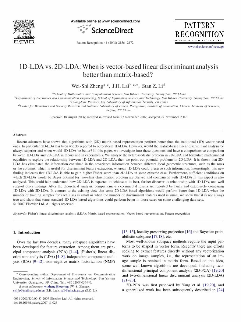
Fig. 1. Illustrations of some face images (images are resized to show): (a) FERET; (b) CMU-Illumination-Frontal; (c) CMU-NearFrontalPose-Expression;(d) CMU-11-Poses.

performed here. The main goal is to compare them under thecase when the number of training samples for each class is lim-ited or when the number of discriminant features used is small.Some existing views will be broken. Experimental results arereported on FERET [55] and CMU [56] databases. As either2D-LDA or 1D-LDA is actually used for discriminant featureextraction, a final classifier is employed for classification in thefeature space. Two such classifiers, namely nearest neighborclassifier (NNC) and nearest class mean classifier (NCMC) areemployed to evaluate the performances. They are always pop-ularly used for evaluation of the LDA-based algorithms and itwill be shown that the final classifier would have an impact onthe performances of some algorithms. Note that in almost allpublished papers regarding 2D-LDA only NNC is selected asthe final classifier [21–23,27,29,30].

We compare some standard 1D-LDA based algorithms withsome standard 2D-LDA based algorithms. The compared 1D-LDA based algorithms involve Fisherface, nullspace LDA andregularized LDA. For comparison, they are renamed as “1D-LDA, Fisherface”, “1D-LDA, nullspace LDA” and “1D-LDA,regularized LDA”. Regularized LDA is implemented by equal-ity (2) with � = 0.005. For 2D-LDA, we have implemented itsthree standard algorithms, i.e., equalities (3)–(5). For compari-son, they are also renamed as “unilateral 2D-LDA, left” (equal-ity (3)), “unilateral 2D-LDA, right (equality (4)), and “bilateral2D-LDA” (equality (5)), where the number of iteration in “bi-lateral 2D-LDA” is set to be 10. Noting that regularized LDAis almost a pure 1D-LDA except the regularization term addedto the within-class scatter matrix, hence it is valuable to take itinto comparison.

4.1. Introduction to databases and subsets

A large subset of FERET [55] is established by extract-ing images from four different sets, namely Fa, Fb, Fc and


duplicate. It consists of 255 persons, and for each individualthere are four face images undergoing expression variation,illumination variation, age variation, etc.

Three subsets of CMU PIE [56] are also established, called“CMU-NearFrontalPose-Expression”, “CMU-Illumination-Frontal” and “CMU-11-Poses”. The subset “CMU-Near-FrontalPose-Expression” is established by selecting imagesunder natural illumination for all persons from the frontalview, 1

4 left\right profile and below\above in frontal view. Foreach view, there are three different expressions, namely natu-ral expression, smiling and blinking [56]. Hence there are 15face images for each object. The subset “CMU-Illumination-frontal” consists of images with all illumination variations inFrontal view under the background light off and on. The subset“CMU-11-Poses” consists of images across 11 different posesof each person, including 3

4 right profile, half right profile,14 right profile, frontal view, 1

4 left profile, half left profile,34 left profile, below in frontal view, above in frontal viewand two surveillance views, and all images are under naturalillumination and natural expression.

The data sets used are briefly summarized in Table 1 andsome face images are illustrated in Fig. 1. Note that all imagesare linearly stretched to full range of pixel values of [0, 1].

Table 2Range of the number of training samples for each class

Database Range

FERET [2 : 1 : 3]CMU-NearFrontalPose-Expression [2 : 1 : 8]a

CMU-Illumination-Frontal [2 : 1 : 8]CMU-11-Poses [2 : 1 : 8]

a[2 : 1 : 8] means the number of training samples for each class rangesfrom 2 to 8 with step 1.

20

30

40

50

60

70

80

Ave

rag

e R

eco

gn

itio

n R

ate

(%

)

1D-LDA, Fisherface

Bilateral 2D-LDA

1D-LDA, NullspaceLDA

Unilateral 2D-LDA, Right

1D-LDA, Regularized LDA

Unilateral 2D-LDA, Left

50

20

30

40

50

60

70

80

Ave

rag

e R

eco

gn

itio

n R

ate

(%

)

1D-LDA, Fisherface

Bilateral 2D-LDA

1D-LDA, Nullspace LDA




Number of Discriminant FeaturesNumber of Discriminant Features

25020015010050 100 150 200 250

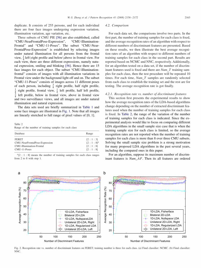
Fig. 2. Recognition rate vs. number of discriminant features on FERET; training number is three for each class. (a) Final classifier: NCMC. (b) Final classifier:NNC.

4.2. Comparison

For each data set, the comparisons involve two parts. In thefirst part, the number of training samples for each class is fixed,and the average recognition rates of an algorithm with respect todifferent numbers of discriminant features are presented. Basedon these results, we then illustrate the best average recogni-tion rates of an algorithm with respect to different numbers oftraining samples for each class in the second part. Results arereported based on NCMC and NNC, respectively. Additionally,for an algorithm tested on a data set, if the number of discrim-inant features used is fixed and there are Num_T training sam-ples for each class, then the test procedure will be repeated 10times. For each time, Num_T samples are randomly selectedfrom each class to establish the training set and the rest are fortesting. The average recognition rate is got finally.

4.2.1. Recognition rate vs. number of discriminant featuresThis section first presents the experimental results to show

how the average recognition rates of the LDA-based algorithmschange depending on the number of extracted discriminant fea-tures used when the number of training samples for each classis fixed. In Table 2, the range of the variation of the numberof training samples for each class is indicated. Since the ex-perimental analysis would like to focus on comparing differentLDA algorithms in the small sample size case that is when thetraining sample size for each class is limited, so the averagerecognition rates are not reported when the number of trainingsamples for each class is more than 8 over three CMU subsets.Solving the small sample size problem is a strong motivationfor many proposed LDA algorithms in the past several years,including the compared ones in this paper.

For an algorithm, suppose its maximum number of discrim-inant features is Num_AF . Then its all features are ordered


10 20 30 40 50 60 70 80

35

40

45

50

55

60

Avera

ge R

ecognitio

n R

ate

(%

)

1D-LDA, Fisherface

Bilateral 2D-LDA




Unilateral 2D-LDA,Left

10 20 30 40 50 60 70 80

30

35

40

45

50

55

60

Avera

ge R

ecognitio

n R

ate

(%

)

1D-LDA, Fisherface

Bilateral 2D-LDA





10 20 30 40 50 60 70 80

40

50

60

70

80

90

Number of Discriminant Features

Avera

ge R

ecognitio

n R

ate

(%

)

1D-LDA, Fisherface

Bilateral 2D-LDA





10 20 30 40 50 60 70 80

40

50

60

70

80

90

Number of Discriminant Features

Avera

ge R

ecognitio

n R

ate

(%

)

1D-LDA, Fisherface

Bilateral 2D-LDA





Number of Discriminant Features Number of Discriminant Features

Fig. 3. Recognition rate vs. number of discriminant features on “CMU-NearFrontalPose-Expression”; training number is two for each class in (a)–(b) andtraining number is seven for each class in (c)–(d). (a) Final classifier: NCMC. (b) Final classifier: NNC. (c) Final classifier: NCMC. (d) Final classifier: NNC.

according to their corresponding eigenvalues in a descen-dant order, since the eigenvalue of each feature could betreated as a measurement of the discriminative ability. Fi-nally, the top Num_F features are selected to evaluate therecognition performance, where we would let Num_F =5, 10, 15, 20, . . . , Num_AF . Additionally, the scheme for“bilateral 2D-LDA” is explained as follows. “bilateral 2D-LDA” has bilateral projections, while the maximum numbersof features with respect to two different side projections arealways different. Hence, if there are Num_F features selectedfor “bilateral 2D-LDA”, it means the top Num_F features areselected for both projections, respectively. If the value Num_F

has exceeded the maximum number of features of one of theprojections, then all features of that projection would be used.

Due to the limited length of the paper, only some fig-ures describe the experiment results could be illustrated. ForFERET database, we present the results when the number oftraining samples for each class is three (Fig. 2); for “CMU-

NearFrontalPose-Expression” and “CMU-11-Poses”, it is 2and 7 in Figs. 3 and 5; for “CMU-Illumination-Frontal” it is 3and 7 in Fig. 4. The sample size of FERET is limited so weonly present the case when the number of training samples foreach class is three; for “CMU-Illumination-Frontal” the resultwhen the number of training samples for each class is 3 ratherthan 2 is presented, because the performance of Fisherfaceincreases notably as observed later in Fig. 7 when NCMC isused. The best average recognition rates with respect to differ-ent numbers of training samples for each class will be totallyreported in the next section.

From the experimental results above, it could observed thatthe 2D-LDA based algorithms always achieve their best perfor-mances when the number of discriminant features is retainedappropriately small while the performances of them wouldsometimes degrade if more features are used. Interestingly, the1D-LDA based algorithms may also achieve their best perfor-mances sometimes when an appropriately small set of features


10 20 30 40 50 60 70 80

55

60

65

70

75

80

Avera

ge R

ecognitio

n R

ate

(%

)

1D-LDA, Fisherface

Bilateral 2D-LDA





10 20 30 40 50 60 70 80

55

60

65

70

75

80

Avera

ge R

ecognitio

n R

ate

(%

)

1D-LDA, Fisherface

Bilateral 2D-LDA





70

75

80

85

90

95

Avera

ge R

ecognitio

n R

ate

(%

)

1D-LDA, Fisherface

Bilateral 2D-LDA




Unilateral 2D-LDA, Left 70

75

80

85

90

Avera

ge R

ecognitio

n R

ate

(%

)

1D-LDA, Fisherface

Bilateral 2D-LDA






10 20 30 40 50 60 70 80 10 20 30 40 50 60 70 80


Fig. 4. Recognition rate vs. number of discriminant features on “CMU-Illumination-Frontal”; training number is three for each class in (a)–(b) and trainingnumber is seven for each class in (c)–(d). (a) Final classifier: NCMC. (b) Final classifier: NNC. (c) Final classifier: NCMC. (d) Final classifier: NNC.

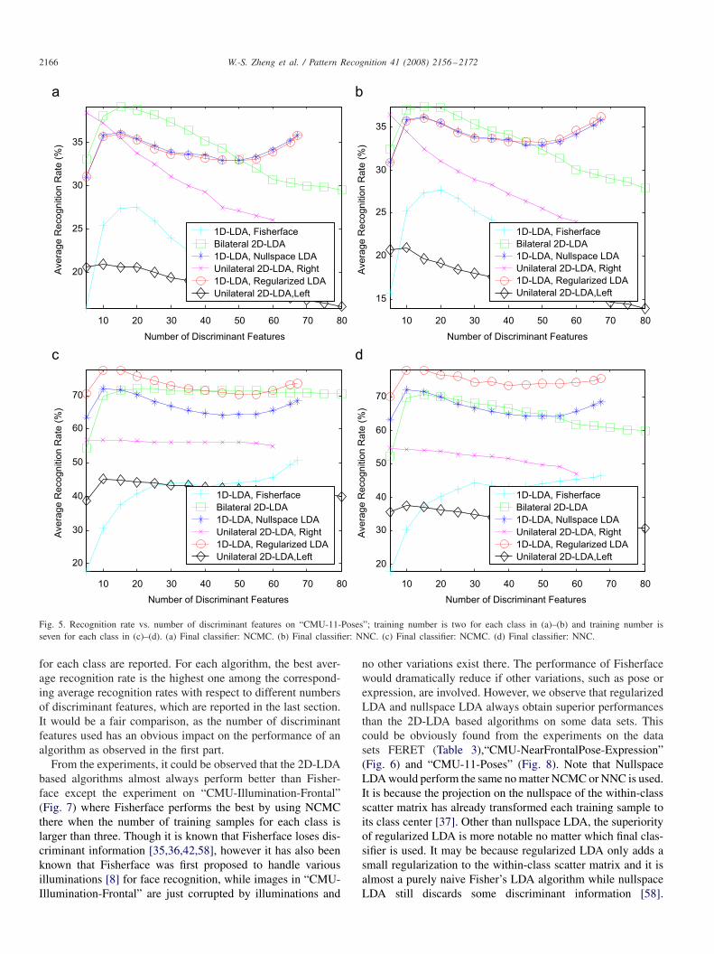
is retained. However, sometimes their performances would firstdescend and then ascend as more features are used. Such sce-nario could be obviously observed in Fig. 3(a)–(b) and Fig. 5.A recent developed theory on LDA by Martínez and Zhu hastold the fact that not all discriminant features are good for clas-sification [57]. Hence a small set of features would sometimesget its best accuracy. Of course it is not always the case, sincethe 2D-LDA based algorithms do not degrade too much in Fig.3(c)–(d) when more features are used and the 1D-LDA basedalgorithms perform better and better in Fig. 4 when more fea-tures are used. However, it could be found that if all features ofthe 1D-LDA based algorithms are used, the performances arealways almost the same as their best ones acquired, but it is notalways the case for the 2D-LDA based algorithms. Therefore,the experimental results indicate how to select the proper num-ber of features would potentially be a more serious problem forthe 2D-LDA based algorithms than that for the 1D-LDA basedalgorithms.

The experiments have also broken the existing viewpoint that2D-LDA could always achieve better performance than 1D-LDA when only fewer discriminant features are used [21,22],since it is also found that regularized LDA and nullspace LDAcould achieve their best performances and perform better thanthe 2D-LDA based algorithms on data sets FERET (Fig. 2),“CMU-NearFrontalPose-Expression” (Fig. 3) and “CMU-11-Poses” (Fig. 5(c)–(d)) when fewer features are used. Note thateven Fisherface could perform better than some 2D-LDA basedalgorithms if a little more discriminant features are employedsometimes.

4.2.2. Recognition rate vs. number of training samplesThis section shows how the best average recognition rate of

an algorithm changes depending on the number of training sam-ples for each class. Except FERET database, all experimentalresults are presented in figures. In all tables and figures, the bestaverage recognition rates for fixed number of training samples


10 20 30 40 50 60 70 80

20

25

30

35

Ave

rag

e R

eco

gn

itio

n R

ate

(%

)

1D-LDA, Fisherface

Bilateral 2D-LDA





10 20 30 40 50 60 70 80

15

20

25

30

35

Ave

rag

e R

eco

gn

itio

n R

ate

(%

)

1D-LDA, Fisherface

Bilateral 2D-LDA





10 20 30 40 50 60 70 80

20

30

40

50

60

70

Ave

rag

e R

eco

gn

itio

n R

ate

(%

)

1D-LDA, Fisherface

Bilateral 2D-LDA





10 20 30 40 50 60 70 80

20

30

40

50

60

70

Ave

rag

e R

eco

gn

itio

n R

ate

(%

)

1D-LDA, Fisherface

Bilateral 2D-LDA







Fig. 5. Recognition rate vs. number of discriminant features on “CMU-11-Poses”; training number is two for each class in (a)–(b) and training number isseven for each class in (c)–(d). (a) Final classifier: NCMC. (b) Final classifier: NNC. (c) Final classifier: NCMC. (d) Final classifier: NNC.

for each class are reported. For each algorithm, the best aver-age recognition rate is the highest one among the correspond-ing average recognition rates with respect to different numbersof discriminant features, which are reported in the last section.It would be a fair comparison, as the number of discriminantfeatures used has an obvious impact on the performance of analgorithm as observed in the first part.

From the experiments, it could be observed that the 2D-LDAbased algorithms almost always perform better than Fisher-face except the experiment on “CMU-Illumination-Frontal”(Fig. 7) where Fisherface performs the best by using NCMCthere when the number of training samples for each class islarger than three. Though it is known that Fisherface loses dis-criminant information [35,36,42,58], however it has also beenknown that Fisherface was first proposed to handle variousilluminations [8] for face recognition, while images in “CMU-Illumination-Frontal” are just corrupted by illuminations and

no other variations exist there. The performance of Fisherfacewould dramatically reduce if other variations, such as pose orexpression, are involved. However, we observe that regularizedLDA and nullspace LDA always obtain superior performancesthan the 2D-LDA based algorithms on some data sets. Thiscould be obviously found from the experiments on the datasets FERET (Table 3),“CMU-NearFrontalPose-Expression”(Fig. 6) and “CMU-11-Poses” (Fig. 8). Note that NullspaceLDA would perform the same no matter NCMC or NNC is used.It is because the projection on the nullspace of the within-classscatter matrix has already transformed each training sample toits class center [37]. Other than nullspace LDA, the superiorityof regularized LDA is more notable no matter which final clas-sifier is used. It may be because regularized LDA only adds asmall regularization to the within-class scatter matrix and it isalmost a purely naive Fisher’s LDA algorithm while nullspaceLDA still discards some discriminant information [58].


Table 3Best average recognition rate on FERET

Final classifier NCMC (%) NNC (%)

Number of training samples for each class 2 3 2 3

1D-LDA, Fisherface 63.51 76.20 63.59 71.611D-LDA, nullspace LDA 76.10 85.10 76.10 85.101D-LDA, regularized LDA 77.35 87.53 77.37 88.27Bilateral 2D-LDA 75.84 83.33 76.29 87.14Unilateral 2D-LDA, right 65.63 70.12 68.78 81.18Unilateral 2D-LDA, left 73.51 81.29 72.51 83.10

2 3 4 5 6 7 8

50

60

70

80

90

Best A

vera

ge R

ecognitio

n R

ate

(%

)

1D-LDA, Fisherface

Bilateral 2D-LDA





2 3 4 5 6 7 8

50

60

70

80

90

Best A

vera

ge R

ecognitio

n R

ate

(%

)

1D-LDA, Fisherface

Bilateral 2D-LDA





Number of Training Samples for Each Class Number of Training Samples for Each Class

Fig. 6. Recognition rate vs. number of training samples on “CMU-NearFrontalPose-Expression”. (a) Final classifier: NCMC. (b) Final Classifier: NNC.

2 3 4 5 6 7 8

60

65

70

75

80

85

90

95

Best A

vera

ge R

ecognitio

n R

ate

(%

)

1D-LDA, Fisherface

Bilateral 2D-LDA





2 3 4 5 6 7 8

60

65

70

75

80

85

90

95

Best A

vera

ge R

ecognitio

n R

ate

(%

)

1D-LDA, Fisherface

Bilateral 2D-LDA





Number of Training Samples for Each ClassNumber of Training Samples for Each Class

Fig. 7. Recognition rate vs. number of training samples on “CMU-Illumination-Frontal”. (a) Final classifier: NCMC; (b) Final classifier: NNC.

Actually, some 2D-LDA based algorithms do not perform wellover some challenging data sets. For instance, both “unilateral2D-LDA, left” and “unilateral 2D-LDA, right” do not have sat-isfied performances on “CMU-NearFrontalPose-Expression”and “CMU-11-Poses” no matter if NCMC or NNC is used, and

“unilateral 2D-LDA, right” does not perform well over “CMU-Illumination-Frontal” using NCMC. However, “bilateral2D-LDA” would perform more stable. It outperforms some1D-LDA based algorithms on “CMU-Illumination-Frontal”data set, and it performs the best especially when only two


2 3 4 5 6 7 8

30

40

50

60

70

Be

st

Ave

rag

e R

eco

gn

itio

n R

ate

(%

)

1D-LDA, Fisherface

Bilateral 2D-LDA





2 3 4 5 6 7 8

30

40

50

60

70

80

Be

st

Ave

rag

e R

eco

gn

itio

n R

ate

(%

)

1D-LDA, Fisherface

Bilateral 2D-LDA





Number of Training Samples for Each Class Number of Training Samples for Each Class

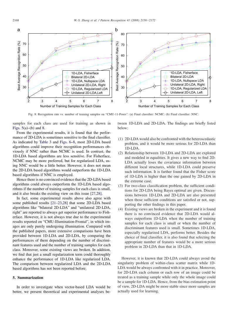
Fig. 8. Recognition rate vs. number of training samples on “CMU-11-Poses”. (a) Final classifier: NCMC. (b) Final classifier: NNC.

samples for each class are used for training as shown inFigs. 5(a)–(b) and 8.

From the experimental results, it is found that the perfor-mance of 2D-LDA is sometimes sensitive to the final classifier.As indicated by Table 3 and Figs. 6–8, most 2D-LDA basedalgorithms could improve their recognition performances ob-viously if NNC rather than NCMC is used. In contrast, the1D-LDA based algorithms are less sensitive. For Fisherface,NCMC may be more preferred, but for regularized LDA, us-ing NNC would be a little better. However, it does not meanthe 2D-LDA based algorithms would outperform the 1D-LDAbased algorithms if NNC is employed.

Hence there is no convinced evidence that the 2D-LDA basedalgorithms could always outperform the 1D-LDA based algo-rithms if the number of training samples for each class is small,and it also breaks the existing view on this issue [27,28].

In fact, some experimental results above also agree withsome published results [21–23,28] that some 2D-LDA basedalgorithms like “bilateral 2D-LDA” and “unilateral 2D-LDA,right” are reported to always get superior performance to Fish-erface. However, it is not always true due to the experimentalresults reported on “CMU-Illumination-Frontal”, in which im-ages are only purely undergoing illumination. Compared withthe published papers, more extensive comparisons have beenprovided between 1D-LDA and 2D-LDA, by comparing theperformances of them depending on the number of discrimi-nant features used and the number of training samples for eachclass. Moreover, some existing views are broken. In addition,we find that just a small regularization term could thoroughlyenhance the performance of 1D-LDA like regularized LDA.The comparison between regularized LDA and the 2D-LDAbased algorithms has not been reported before.

5. Summarization

In order to investigate when vector-based LDA would bebetter, we present theoretical and experimental analyses be-

tween 1D-LDA and 2D-LDA. The findings are briefly listedbelow:

(1) 2D-LDA would also be confronted with the heteroscedasticproblem, and it would be more serious for 2D-LDA than1D-LDA.

(2) Relationship between 1D-LDA and 2D-LDA are exploredand modeled in equalities. It gives a new way to find 2D-LDA actually loses the covariance information betweendifferent local structures, while 1D-LDA could preservesuch information. It is further found that the Fisher scoreof 1D-LDA is higher than the one gained by 2D-LDA inthe extreme case.

(3) For two-class classification problem, the sufficient condi-tions for 2D-LDA being Bayes optimal are given. Discus-sions between 1D-LDA and 2D-LDA are also presentedwhen those sufficient conditions are satisfied or not, sup-porting the other findings in this paper.

(4) Existing views are broken in the experiment and it is foundthere is no convinced evidence that 2D-LDA would al-ways outperform 1D-LDA when the number of trainingsamples for each class is small or when the number ofdiscriminant features used is small. Sometimes 1D-LDA,especially regularized LDA, performs better. Besides thechoice of final classifier, it is also found that selecting theappropriate number of features would be a more seriousproblem in 2D-LDA than that in 1D-LDA.

However, it is known that 2D-LDA could always avoid thesingularity problem of within-class scatter matrix while 1D-LDA would be always confronted with it in practice. Moreover,for 2D-LDA each column or each row of an image could betreated as a training sample while only the whole image couldbe a sample for 1D-LDA. Hence, from the bias estimation pointof view, 2D-LDA might be more stable since more samples areactually used for learning.


Finally, it is stressed that this paper does not aim to declarewhich algorithm is the best. We investigate into the question bypresenting a fair comparison between 1D-LDA and 2D-LDAin both theoretical and experimental sense. The goal of theextensive comparisons is to explore the properties of 2D-LDA,present its disadvantages and some inherent problems, and findwhen 1D-LDA would be better. Even though some 2D-LDAbased algorithms do not perform as well as some standard 1D-LDA based algorithms in the experiments, it still does not mean2D-LDA is not effective sometimes.

In conclusion, our findings indicate that using the matrix-based feature extraction technique would not always result in abetter performance than using the traditional vector-form rep-resentation. The traditional vector-form representation is stilluseful.

Acknowledgements

This project was supported by the National NaturalScience Foundation of China (60373082), 973 Program(2006CB303104), the Key (Key grant) Project of ChineseMinistry of Education (105134) and NSF of Guangdong(06023194). The authors would also like to thank the reviewersfor their constructive advice.

Appendix A. Proof of Lemma 1

As indicated at the beginning of Section 3, we note thatxki = [Xk

i (1)T, . . . , Xki (col)T]T. Then we have

wTSbw

=L∑

k=1

Nk

NwT(uk − u)(uk − u)Tw

=L∑

k=1

Nk

N[�wT

1 , . . . ,�w

T

col]⎡⎣ Uk(1) − U(1)

...

Uk(col) − U(col)

⎤⎦

× [(Uk(1) − U(1))T, . . . , (Uk(col) − U(col))T]⎡⎣

�w1...

�wcol

⎤⎦

=L∑

k=1

Nk

N

⎡⎣ col∑

j=1

�w

T

j (Uk(j) − U(j))

⎤⎦

×⎡⎣ col∑

j=1

(Uk(j) − U(j))T�wj

⎤⎦

=L∑

k=1

Nk

N

col∑j=1

�w

T

j (Uk(j) − U(j))(Uk(j) − U(j))T�wj

+L∑

k=1

Nk

N


�w

T

j (Uk(j) − U(j))(Uk(h)

− U(h))T�wh, (A.1)

wTSww

= 1

N

L∑k=1

Nk∑i=1

wT(xki − uk)(xk

i − uk)Tw

= 1

N

L∑k=1

Nk∑i=1

[�wT

1 , . . . ,�w

T

col]⎡⎢⎣

Xki (1) − Uk(1)

...

Xki (col) − Uk(col)

⎤⎥⎦

× [(Xki (1) − Uk(1))T, . . . , (Xk

i (col) − Uk(col))T]

×⎡⎣

�w1...

�wcol

⎤⎦

= 1

N

L∑k=1

Nk∑i=1

⎡⎣ col∑

j=1

�w

T

j (Xki (j) − Uk(j))

⎤⎦

×⎡⎣ col∑

j=1

(Xki (j) − Uk(j))T�

wj

⎤⎦

= 1

N

L∑k=1

Nk∑i=1

col∑j=1

�w

T

j (Xki (j) − Uk(j))(Xk

i (j) − Uk(j))T�wj

+ 1

N

L∑k=1

Nk∑i=1


�w

T

j (Xki (j) − Uk(j))(Xk

i (h)

− Uk(h))T�wh. (A.2)

Using equalities (6)–(7) and equalities (8), (11), the lemma isthen proved.

Appendix B. Proof of Theorem 2

Based on equalities (21)–(23), substituting the estimatesof the means and the covariance matrices and eliminating theineffective ingredients that do not affect the classification resultin formula (21) would yield the following Bayes classifier:

gk(X) =col∑j=1

{−1

2log |�̂j

k | − 1

2(X(j) − Uk(j))T(�̂j

k )−1(X(j)

−Uk(j))

}+ log(P (Ck)). (B.1)

Under the condition (2) in the theorem, �̂jk are equal. We hence

further have

gk(X) =col∑j=1

{−1

2log |S̃w| − 1

2(X(j) − Uk(j))T(S̃w)−1(X(j)

−Uk(j))

}+ log(P (Ck))

=col∑j=1

{−1

2log |S̃w| − 1

2(X(j))T(S̃w)−1X(j)

+ (Uk(j))T(S̃w)−1X(j)

−1

2(Uk(j))T(S̃w)−1Uk(j)

}+ log(P (Ck)).


By eliminating the ineffective terms again, the Bayes classifiergk(X) could be further reduced and formulated as

gk(X)=col∑j=1

{(Uk(j))T(S̃w)−1X(j) − 1

2(Uk(j))T(S̃w)−1Uk(j)

}+ log(P (Ck)) (B.2)

Therefore, for two-class classification, it is said X ∈ C1 if andonly if g1(X) > g2(X), i.e.,

col∑j=1

{(U1(j))T(S̃w)−1X(j) − 1

2(U1(j))T(S̃w)−1U1(j)

}+ log(P (C1))

>

col∑j=1

{(U2(j))T(S̃w)−1X(j)− 1

2(U2(j))T(S̃w)−1U2(j)

}+ log(P (C2)).

Then we could say X ∈ C1 if and only if

col∑j=1

wTj X(j) + w0 > 0,

wj = (S̃w)−1(U1(j) − U2(j)),

w0 =col∑j=1

−1

2(U1(j)

+ U2(j))T(S̃w)−1(U1(j) − U2(j)) + logP(C1)

P (C2).

(B.3)

Finally, under the condition (3) in the theorem, i.e., �U =si(U1(i)−U2(i))=sj (U1(j)−U2(j)), ∀i �= j, i, j=1, . . . , col,we then obtain the declaration that X ∈ C1 if and only if

wTbayes

⎛⎝ col∑

j=1

(sj )−1X(j)

⎞⎠+ w0 > 0,

wbayes = w1 = · · · = wcol = (S̃w)−1�U (B.4)

else X ∈ C2.Next, the following shows why 2D-LDA in terms of equal-

ity (3) would be a Bayes optimal feature extractor for two-class classification problem under the conditions indicated inTheorem 2. First, for two-class classification problem, S2d

b =∑colj=1 S2d

b,j and S2dw =∑col

j=1 S2dw,j , where

S2db,j = N1

N(U1(j) − U(j))(U1(j) − U(j))T + N2

N(U2(j)

− U(j))(U2(j) − U(j))T,

U(j) = N1

NU1(j) + N2

NU2(j),

S2dw,j = 1

N

2∑k=1

Nk∑i=1


i (j) − Uk(j))T,

j = 1, . . . , col.

Note that S2db,j and S2d

b could be written equivalently belowbased on N = N1 + N2 and equality (25):

S2db,j = N1N2

N2 (U1(j) − U2(j))(U1(j) − U2(j))T

= N1N2

N2 (sj )−2�U(�UT),

S2db =

col∑j=1

S2db,j = N1N2

N2 �U

⎛⎝ col∑

j=1

(sj )−2�UT

⎞⎠ .

Second, it is known that the optimal feature of 2D-LDA interms of equality (3) for two-class classification problem wouldsatisfy �optw2d

opt = (S2dw )−1S2d

b w2dopt , �opt > 0. Hence we have

w2dopt = (�opt )

−1(S2dw )−1 N1N2

N2 �U

⎛⎝ col∑

j=1

(sj )−2�UT

⎞⎠w2d

opt .

(B.5)

Since (�opt )−1 N1N2

N2 (∑col

j=1 (sj )−2�UT)w2d

opt is a scalar value,then we have

w2dopt ∝ (S2d

w )−1�U. (B.6)

Furthermore, it is easy to verify S2dw =col · S̃w. Comparing with

equality (B.4), we then have

w2dopt ∝ wbayes . (B.7)

It means the discriminant feature of 2D-LDA is in proportionto the Bayes optimal feature obtained in equality (B.4). Theyare the same except some scalar scaling under the conditionsindicated by the theorem.

References

[1] M. Kirby, L. Sirovich, Application of the KL procedure for thecharacterization of human faces, IEEE Trans. Pattern Anal. Mach. Intell.12 (1) (1990) 103–108.

[2] M. Turk, A. Pentland, Eigenfaces for recognition, J. Cognitive Neurosci.3 (1) (1991) 71–86.

[3] A.M. Martinez, A.C. Kak, PCA versus LDA, IEEE Trans. Pattern Anal.Mach. Intell. 23 (2) (2001) 228–233.

[4] K. Fukunnaga, Introduction to Statistical Pattern Recognition, seconded., Academic Press, New York, 1991.

[5] A.R. Webb, Statistical Pattern Recognition, second ed., Wiley, New York,2002.

[6] R.A. Fisher, The use of multiple measures in taxonomic problems, Ann.Eugenics 7 (1936) 179–188.

[7] D.L. Swets, J. Weng, Using discriminant eigenfeatures for imageretrieval, IEEE Trans. Pattern Anal. Mach. Intell. 18 (8) (1996) 831–836.

[8] P.N. Belhumeur, J. Hespanha, D.J. Kriegman, Eigenfaces vs. Fisherfaces:recognition using class specific linear projection, IEEE Trans. PatternAnal. Mach. Intell. 19 (7) (1997) 711–720.

[9] P. Comon, Independent component analysis, a new concept?, SignalProcessing 36 (1994) 287–314.

[10] A. Hyvärinen, J. Karhunen, E. Oja, Independent Component Analysis,Wiley, New York, 2001.

[11] P.C. Yuen, J.H. Lai, Face representation using independent componentanalysis, Pattern Recognition 35 (6) (2002) 1247–1257.

[12] M.S. Bartlett, J.R. Movellan, T.J. Sejnowski, Face recognition byindependent component analysis, IEEE Trans. Neural Networks 13 (6)(2002) 1450–1464.


[13] D.D. Lee, H.S. Seung, Learning the parts of objects by non-negativematrix factorization, Nature 401 (6755) (1999) 788–791.

[14] S.Z. Li, X.W. Hou, H.J. Zhang, Learning spatially localized, parts-basedrepresentation, in: CVPR, 2001.

[15] A. Pascual-Montano, J.M. Carazo, K. Kochi, D. Lehmann, R.D. Pascual-Marqui, Nonsmooth nonnegative matrix factorization (nsNMF), IEEETrans. Pattern Anal. Mach. Intell. 28 (3) (2006) 403–415.

[16] X. He, S. Yan, Y. Hu, P. Niyogi, H.-J. Zhang, Face recognition usingLaplacianfaces, IEEE Trans. Pattern Anal. Mach. Intell. 27 (3) (2005)328–340.

[17] B. Moghaddam, Principle manifolds and probabilistic subspace for visualrecognition, IEEE Trans. Pattern Anal. Mach. Intell. 24 (6) (2002)780–788.

[18] B. Moghaddam, T. Jebara, A. Pentland, Bayesian face recognition, PatternRecognition 33 (2000) 1771–1782.

[19] J. Yang, D. Zhang, A.F. Frangi, J. Yang, Two-dimensional PCA: a newapproach to appearance-based face representation and recognition, IEEETrans. Pattern Anal. Mach. Intell. 26 (1) (2004) 131–137.

[20] J. Yang, J.Y. Yang, From image vector to matrix: a straightforwardimage projection technique—IMPCA vs. PCA, Pattern Recognition 35(9) (2002) 1997–1999.

[21] M. Li, B. Yuan, 2D-LDA: a novel statistical linear discriminant analysisfor image matrix, Pattern Recognition Lett. 26 (5) (2005) 527–532.

[22] H. Xiong, M.N.S. Swamy, M.O. Ahmad, Two-dimensional FLD for facerecognition, Pattern Recognition 38 (2005) 1121–1124.

[23] J. Ye, R. Janardan, Q. Li, Two-dimensional linear discriminant analysis,in: NIPS, 2004.

[24] H. Kong, L. Wang, E.K. Teoh, J.G. Wang, V. Ronda, Generalized 2Dprincipal component analysis, in: IEEE Conference on IJCNN, Canada,2005.

[25] J. Ye, Generalized low rank approximations of matrices, Mach. Learn.61 (2005) 167–191.

[26] D. Zhang, Z.-H. Zhou, S. Chen, Diagonal principal component analysisfor face recognition, Pattern Recognition 39 (2006) 140–142.

[27] J. Yang, D. Zhang, X. Yong, J.-Y. Yang, Two-dimensional discriminanttransform for face recognition, Pattern Recognition 38 (2005)1125–1129.

[28] H. Kong, L. Wang, E.K. Teoh, A framework of 2D Fisher discriminantanalysis: application to face recognition with small number of trainingsamples, in: CVPR, 2005.

[29] S. Noushatha, G. Hemantha Kumar, P. Shivakumara, (2D)2 LDA: anefficient approach for face recognition, Pattern Recognition 39 (2006)1396–1400.

[30] X.-Y. Jing, H.-S. Wong, D. Zhang, Face recognition based on 2DFisherface approach, Pattern Recognition, 39 (2006) 707–710.

[31] N.V. Chawla, K. Bowyer, Random subspaces and subsampling for 2-Dface recognition, in: CVPR, 2005.

[32] K. Liu, Y.-Q. Cheng, J.-Y. Yang, Algebraic feature extraction forimage recognition based on an optimal discriminant criterion, PatternRecognition 26 (6) (1993) 903–911.

[33] L. Wang, X. Wang, J. Feng, On image matrix based feature extractionalgorithms, IEEE Trans. Syst Man Cybern.—Part B: Cybern. 36 (1)(2006) 194–197.

[34] D. Xu, S. Yan, L. Zhang, M. Li, W. Ma, Z. Liu, H. Zhang, Parallelimage matrix compression for face recognition, in: Proceedings of the11th International Multimedia Modelling Conference, 2005.

[35] L. Chen, H. Liao, M. Ko, J. Lin, G. Yu, A new LDA based facerecognition system which can solve the small sample size problem,Pattern Recognition 33 (10) (2000) 1713–1726.

[36] R. Huang, Q.S. Liu, H.Q. Lu, S.D. Ma, Solving the small sample sizeproblem of LDA, in: ICPR, 2002.

[37] H. Cevikalp, M. Neamtu, M. Wilkes, A. Barkana, Discriminative commonvectors for face recognition, IEEE Trans. Pattern Anal. Mach. Intell. 27(1) (2005) 4–13.

[38] J. Ye, R. Janardan, C.H. Park, H. Park, An optimization criterionfor generalized discriminant analysis on undersampled problems, IEEETrans. Pattern Anal. Mach. Intell. 26 (8) (2004) 982–994.

[39] M. Loog, R.P.W. Duin, Linear dimensionality reduction via aheteroscedastic extension of LDA: the Chernoff criterion, IEEE Trans.Pattern Anal. Mach. Intell. 26 (6) (2004) 732–739.

[40] W.-S. Zheng, J.-H. Lai, P.C. Yuen, GA-fisher: a new LDA-based facerecognition algorithm with selection of principal components, IEEETrans. Syst. Man Cybern. Part B 35 (5) (2005) 1065–1078.

[41] C. Liu, H. Wechsler, Enhanced Fisher linear discriminant models forface recognition, in: ICPR, 1998.

[42] H. Yu, J. Yang, A direct LDA algorithm for high dimensional datawith application to face recognition, Pattern Recognition 34 (10) (2001)2067–2070.

[43] J. Ye, Q. Li, LDA/QR: an efficient and effective dimension reductionalgorithm and its theoretical foundation, Pattern Recognition 37 (2004)851–854.

[44] W. Zhao, R. Chellappa, P.J. Phillips, Subspace linear discriminantanalysis for face recognition, Technical Report CAR-TR-914, CS-TR-4009, University of Maryland, College Park, MD.

[45] J. Lu, K.N. Plataniotis, A.N. Venetsanopoulos, Regularization studiesof linear discriminant analysis in small sample size scenarios withapplication to face recognition, Pattern Recognition Letters 26 (2005)181–191.

[46] D.-Q. Dai, P.C. Yuen, Regularized discriminant analysis and itsapplication to face recognition, Pattern Recognition 36 (2003) 845–847.

[47] P. Zhang, J. Peng, N. Riedel, Discriminant analysis: a least squaresapproximation view, in: CVPR, 2005.

[48] Z. Jin, J.Y. Yang, Z.S. Hu, Z. Lou, Face recognition based on theuncorrelated discriminant transformation, Pattern Recognition 34 (2001)1405–1416.

[49] J. Duchene, S. Leclercq, An optimal transformation for discriminant andprincipal component analysis, IEEE Trans. Pattern Anal. Mach. Intell.10 (6) (1988) 978–983.

[50] J.R. Price, T.F. Gee, Face recognition using direct, weighted lineardiscriminant analysis and modular subspaces, Pattern Recognition 38(2005) 209–219.

[51] H.-C. Kim, D. Kim, S.Y. Bang, Face recognition using LDA mixturemodel, Pattern Recognition Lett. 24 (2003) 2815–2821.

[52] T.-K. Kim, J. Kittler, Locally linear discriminant analysis formultimodally distributed classes for face recognition with a single modelimage, IEEE Trans. Pattern Anal. Mach. Intell. 27 (3) (2005) 318–327.

[53] F. De la Torre Frade, T. Kanade, Multimodal oriented discriminantanalysis, in: International Conference on Machine Learning (ICML),August, 2005.

[54] S. Yan, D. Xu, Q. Yang, L. Zhang, X. Tang, H.-J. Zhang, Discriminantanalysis with tensor representation, in: CVPR, 2005.

[55] P.J. Phillips, H. Moon, S.A. Rizvi, P.J. Rauss, The feret evaluationmethodology for face recognition algorithms, IEEE Trans. Pattern Anal.Mach. Intell. 22 (10) (2000) 1090–1104.

[56] T. Sim, S. Baker, M. Bsat, The CMU pose, illumination, and expressiondatabase, IEEE Trans. Pattern Anal. Mach. Intell. 25 (12) (2003)1615–1618.

[57] A.M. Martínez, M. Zhu, Where are linear feature extraction methodsapplicable?, IEEE Trans. Pattern Anal. Mach. Intell. 27 (12) (2005)1934–1944.

[58] J. Yang, J.Y. Yang, Why can LDA be performed in PCA transformedspace?, Pattern Recognition 36 (2) (2003) 563–566.

About the Author—WEI-SHI ZHENG was born in Guangzhou (Canton), China, in 1981. He received the B.S. degree in both mathematics and computerscience at Sun Yat-sen University, Guangzhou, in 2003. He is now pursuing a Ph.D. degree in applied mathematics at Sun Yat-Sen University. From April2006 to October 2006, he was a visiting student at Center for Biometrics and Security Research and National Laboratory of Pattern Recognition, Institute ofAutomation, Chinese Academy of Sciences. In 2007, he has been an exchanged research student at Hong Kong Baptist University from May 16 to November 15.He is a student member of IEEE.His current research interests include pattern recognition, machine learning, and face recognition.


About the Author—J.H. LAI was born in 1964. He received the M.Sc. degree in applied mathematics in 1989 and the Ph.D. degree in mathematics in1999 from Sun Yat-sen University, Guangzhou, China. He joined Sun Yat-sen University in 1989, where currently, he is a Professor with the Department ofElectronics and Communication Engineering, School of Information Science and Technology. He has published over 50 papers in the international journals,book chapters, and conferences. His current research interests are in the areas of digital image processing, pattern recognition, multimedia communication,wavelets and their applications. Dr. Lai had successfully organized the International Conference on Advances in Biometric Personal Authentication’ 2004,which was also the Fifth Chinese Conference on Biometric Recognition (Sinobiometrics’04), Guangzhou, in December 2004. He has taken charge of more thanfour research projects, including NSFC (number 60144001, 60 373 082, 60675016), the Key (Key grant) Project of Chinese Ministry of Education (number105 134), and NSF of Guangdong, China (number 021 766, 06023194). He serves as a board member of the Image and Graphics Association of China andalso serves as a board member and secretary-general of the Image and Graphics Association of Guangdong.

About the Author—STAN Z. LI received the Ph.D. degree from Surrey University, UK, in 1991. He is currently a professor at National Laboratory of PatternRecognition (NLPR), director of Center for Biometrics and Security Research (CBSR), Institute of Automation, Chinese Academy of Sciences (CASIA); anddirector of Joint Laboratory for Intelligent Surveillance and Identification in Civil Aviation (CASIA-CAUC). He worked at Microsoft Research Asia as aresearcher from 2000 to 2004. Prior to that, he was an associate professor at Nanyang Technological University, Singapore. His research interest includesface recognition, biometrics, intelligent video surveillance, pattern recognition and machine learning, and image and video processing. He authored the book“Markov Random Field Modeling in Image Analysis” (Springer, 1st edition in 1995 and 2nd edition in 2001), co-edited “Handbook of Face Recognition”(Springer, 2005), and published over 200 papers in international journals and conferences. He is currently an associated editor of IEEE Transactions on PatternAnalysis and Machine Intelligence. He leads several national and international collaboration projects in biometrics and intelligent video surveillance. He hasbeen actively participating in organizing a number of international conferences and workshops in the fields of computer vision, image processing, patternrecognition, face analysis and biometrics.

1D-LDA vs. 2D-LDA: When is vector-based linear discriminant ...

Documents

Transcript of 1D-LDA vs. 2D-LDA: When is vector-based linear discriminant ...