requirement - arXiv · inequalities, minimum sample size requirement, linear discriminant analysis...

Journal of Machine Learning Research 21 (2020) 1-44 Submitted 8/18; Revised 12/19; Published 1/20

Neyman-Pearson classification: parametrics and sample sizerequirement

Xin Tong [email protected] of Data Sciences and OperationsMarshall Business SchoolUniversity of Southern California

Lucy Xia [email protected] of ISOMSchool of Business and ManagementHong Kong University of Science and Technology

Jiacheng Wang [email protected] of StatisticsUniversity of Chicago

Yang Feng [email protected]

Department of Biostatistics

School of Global Public Health

New York University

Editor: Xiaotong Shen

Abstract

The Neyman-Pearson (NP) paradigm in binary classification seeks classifiers that achieve a min-imal type II error while enforcing the prioritized type I error controlled under some user-specifiedlevel α. This paradigm serves naturally in applications such as severe disease diagnosis and spamdetection, where people have clear priorities among the two error types. Recently, Tong et al.(2018) proposed a nonparametric umbrella algorithm that adapts all scoring-type classificationmethods (e.g., logistic regression, support vector machines, random forest) to respect the giventype I error (i.e., conditional probability of classifying a class 0 observation as class 1 under the0-1 coding) upper bound α with high probability, without specific distributional assumptionson the features and the responses. Universal the umbrella algorithm is, it demands an explicitminimum sample size requirement on class 0, which is often the more scarce class, such as inrare disease diagnosis applications. In this work, we employ the parametric linear discriminantanalysis (LDA) model and propose a new parametric thresholding algorithm, which does notneed the minimum sample size requirements on class 0 observations and thus is suitable forsmall sample applications such as rare disease diagnosis. Leveraging both the existing nonpara-metric and the newly proposed parametric thresholding rules, we propose four LDA-based NPclassifiers, for both low- and high-dimensional settings. On the theoretical front, we prove NPoracle inequalities for one proposed classifier, where the rate for excess type II error benefitsfrom the explicit parametric model assumption. Furthermore, as NP classifiers involve a samplesplitting step of class 0 observations, we construct a new adaptive sample splitting scheme thatcan be applied universally to NP classifiers, and this adaptive strategy reduces the type II errorof these classifiers.

Keywords: classification, asymmetric error, Neyman-Pearson (NP) paradigm, NP oracleinequalities, minimum sample size requirement, linear discriminant analysis (LDA), NP umbrellaalgorithm, adaptive splitting

c©2020 Xin Tong, Lucy Xia, Jiacheng Wang and Yang Feng.

License: CC-BY 4.0, see https://creativecommons.org/licenses/by/4.0/. Attribution requirements are provided athttp://jmlr.org/papers/v21/18-577.html.

arX

iv:1

802.

0255

7v5

[st

at.M

E]

28

Jan

2020

https://creativecommons.org/licenses/by/4.0/

http://jmlr.org/papers/v21/18-577.html

Tong, Xia, Wang and Feng

1. Introduction

Classification aims to predict discrete outcomes (i.e., class labels) for new observations, usingalgorithms trained on labeled data. It is one of the most studied machine learning problems withapplications including automatic disease diagnosis, email spam filters, and image classification.Binary classification, where the outcomes belong to one of two classes and the class labels areusually coded as {0, 1} (or {−1, 1} or {1, 2}), is the most common type. Most binary classifiersare constructed to minimize the overall classification error (i.e., risk), which is a weighted sumof type I and type II errors. Here, type I error is defined as the conditional probability ofmisclassifying a class 0 observation as class 1, and type II error is the conditional probabilityof misclassifying a class 1 observation as class 0 1. In the following, we refer to this paradigmas the classical classification paradigm. Along this line, numerous methods have been proposed,including linear discriminant analysis (LDA) in both low and high dimensions (Guo et al.,2005; Cai and Liu, 2011; Shao et al., 2011; Witten and Tibshirani, 2012; Fan et al., 2012; Maiet al., 2012), logistic regression, support vector machine (SVM) (Vapnik, 1999), random forest(Breiman, 2001), among others.

In contrast, the Neyman-Pearson (NP) classification paradigm (Cannon et al., 2002; Scottand Nowak, 2005; Rigollet and Tong, 2011; Tong, 2013; Zhao et al., 2016; Tong et al., 2016)was developed to seek a classifier that minimizes the type II error while maintaining the typeI error below a user-specified level α, usually a small value (e.g., 5%). We call this targetclassifier the NP oracle classifier. The NP paradigm is appropriate in applications such as cancerdiagnosis, where a type I error (i.e., misdiagnosing a cancer patient to be healthy) has more severeconsequences than a type II error (i.e., misdiagnosing a healthy patient as with cancer). Thelatter incurs extra medical costs and patients’ anxiety but will not result in the tragic loss oflife, so it is appropriate to have type I error control as the priority. Cost-sensitive learning,which assigns different costs as weights of type I and type II errors (Elkan, 2001; Zadroznyet al., 2003) is a popular alternative paradigm to address asymmetric errors. This approach hasmerits and many practical values. However, when there is no consensus to assign costs to errors,or in applications such as medical diagnosis, where it is morally unacceptable to do a cost andbenefit analysis, the NP paradigm is a more natural choice. Previous NP classification literatureuse both empirical risk minimization (ERM) (Cannon et al., 2002; Casasent and Chen, 2003;Scott, 2005; Scott and Nowak, 2005; Han et al., 2008; Rigollet and Tong, 2011) and plug-inapproaches (Tong, 2013; Zhao et al., 2016), and its genetic application is suggested in Li andTong (2016). More recently, Tong et al. (2018) took a different route, and proposed an NPumbrella algorithm that adapts scoring-type classification algorithms (e.g., logistic regression,support vector machines, random forest, etc.) to the NP paradigm, by setting nonparametricorder statistics based thresholds on the classification scores. To implement the NP paradigm, itis very tempting to simply tune the empirical type I error to (no more than) α. Nevertheless,as argued extensively in Tong et al. (2018), doing so would not lead to classifiers whose type Ierrors are bounded from above by α with high probability.

Universal the NP umbrella algorithm is, it demands an explicit minimum sample size re-quirement on class 0, which is usually the more scarce class. While this requirement is not toostringent, it does cause a problem when the smaller class 0 has an insufficient sample size. Forinstance, a commonly-used lung cancer diagnosis example (Gordon et al., 2002) in the high-dimensional statistics literature has 181 subjects and 12, 533 features. These subjects carry two

1. In verbal discussion, with a slight abuse of language, we also refer to the action of assigning a class 0 observationto class 1 as type I error, and that of assigning a class 1 observation to class 0 as type II error.

2

Neyman-Pearson classification: parametrics and sample size requirement

different types of lung cancer, namely, adenocarcinoma (150 subjects) and mesothelioma (31subjects). If we were to treat mesothelioma as the class 0, and would like to control the typeI error under α = .05 with high probability 1 − δ0 = .95, then the sample size requirement ofthe NP umbrella algorithm for the left-out class 0 observations is 59 (or log δ0/ log(1 − α) tobe exact), which is almost twice as much as the total available class 0 sample size 31. In thiswork, we employ the linear discriminant analysis (LDA) model and propose a new thresholdingalgorithm, which does not have the minimum sample size requirements on class 0 observationsand thus applies to small sample applications such as rare disease diagnosis.

In total, we develop four NP classifiers in this paper: combinations of two different waysto create scoring functions in low- and high-dimensional settings under the LDA model, andtwo thresholding methods that include the nonparametric order statistics based NP umbrellaalgorithm and the newly proposed parametric thresholding rule. We will denote these classifiersby NP-LDA, NP-sLDA, pNP-LDA and pNP-sLDA, where p means “parametric thresholding” and s

means “sparse”. Extensive numerical experiments will suggest the recommended applicationdomains of these methods.

On the theoretical front, NP oracle inequalities, a core theoretical criterion to evaluate clas-sifiers under the NP paradigm, were only established for nonparametric plug-in classifiers (Tong,2013; Zhao et al., 2016). The current work is the first to establish NP oracle inequalities underparametric models. Concretely, we will show that NP-sLDA satisfies the NP oracle inequalities.Another major contribution of this work is that we design an adaptive sample splitting schemethat can be applied universally to existing NP classifiers. This adaptive strategy enhances thepower (i.e., reduces type II error) and therefore raises the practicality of the NP algorithms.

The rest of this paper is organized as follows. Section 2 introduces the notations and modelsetup. Section 3 constructs the new parametric thresholding rule based on the LDA model andintroduces four new LDA based NP classifiers. Section 4 formulates theoretical conditions andderives NP oracle inequalities for NP-sLDA. Section 5 describes the new data-adaptive samplesplitting scheme. Numerical results are presented in Section 6, followed by a short discussionin Section 7. Longer proofs, additional numerical results, and other supporting intermediateresults are relegated to the appendices.

2. Notations and model setup

A few standard notations are introduced to facilitate our discussion. Let (X,Y ) be a random pairwhere X ∈ X ⊂ Rd is a d-dimensional vector of features, and Y ∈ {0, 1} indicates X’s class label.Denote respectively by IP and IE generic probability distribution and expectation. A classifierφ : X → {0, 1} is a data-dependent mapping from X to {0, 1} that assigns X to one of theclasses. The overall classification error of φ is R(φ) = IE1I{φ(X) 6= Y } = IP {φ(X) 6= Y }, where1I(·) denotes the indicator function. By the law of total probability, R(φ) can be decomposedinto a weighted average of type I error R0(φ) = IP {φ(X) 6= Y |Y = 0} and type II error R1(φ) =IP {φ(X) 6= Y |Y = 1} as

R(φ) = π0R0(φ) + π1R1(φ) , (1)

where π0 = IP(Y = 0) and π1 = IP(Y = 1). While the classical paradigm minimizes R(·),the Neyman-Pearson (NP) paradigm seeks to minimize R1 while controlling R0 under a user-specified level α. The (level-α) NP oracle classifier is thus

φ∗α ∈ arg minR0(φ)≤α

R1(φ) , (2)

where the significance level α reflects the level of conservativeness towards type I error.

3


In this paper, we assume that (X|Y = 0) and (X|Y = 1) follow multivariate Gaussiandistributions with a common covariance matrix. That is, their probability density functions f0

and f1 aref0 ∼ N (µ0,Σ) and f1 ∼ N (µ1,Σ) ,

where the mean vectors µ0, µ1 ∈ Rd (µ0 6= µ1) and the common positive definite covariancematrix Σ ∈ Rd×d. This model is frequently referred to as the linear discriminant analysis(LDA) model. Despite its simplicity, the LDA model has been proved to be effective in manyapplications and benchmark datasets. Moreover, in the last ten years, several papers (Shaoet al., 2011; Cai and Liu, 2011; Fan et al., 2012; Witten and Tibshirani, 2012; Mai et al., 2012)have developed LDA based algorithms under high-dimensional settings where the dimensionalityof features is comparable to or larger than the sample size.

It is well known that the Bayes classifier (i.e., oracle classifier) of the classical paradigmis φ∗(x) = 1I(η(x) > 1/2), where η(x) = IE(Y |X = x) = IP(Y = 1|X = x) is the regressionfunction. Since

η(x) =π1 · f1(x)/f0(x)

π1 · f1(x)/f0(x) + π0,

the oracle classifier can be written alternatively as 1I(f1(x)/f0(x) > π0/π1). When f0 and f1

follow the LDA model, the oracle classifier of the classical paradigm is

φ∗(x) = 1I

{(x− µa)>Σ−1µd + log

π1

π0> 0

}= 1I

{(Σ−1µd)

>x > µ>a Σ−1µd − logπ1

π0

}, (3)

where µa = 12(µ0 + µ1), µd = µ1 − µ0, and (·)> denotes the transpose of a vector. In con-

trast, motivated by the famous Neyman-Pearson Lemma in hypothesis testing (attached in theAppendix A for readers’ convenience), the NP oracle classifier is

φ∗α(x) = 1I

{f1(x)

f0(x)> Cα

}, (4)

for some threshold Cα such that P0{f1(X)/f0(X) > Cα} ≤ α and P0{f1(X)/f0(X) ≥ Cα} ≥ α,where P0 is the conditional probability distribution of X given Y = 0 (P1 is defined similarly).

Under the LDA model assumption, the NP oracle classifier is φ∗α(x) = 1I((Σ−1µd)>x >

C∗∗α ), where C∗∗α = logCα + µ>a Σ−1µd. Denote by βBayes = Σ−1µd and s∗(x) = (Σ−1µd)>x =

(βBayes)>x, then the NP oracle classifier (4) can be written as

φ∗α(x) = 1I(s∗(x) > C∗∗α ) . (5)

In fact, leveraging further the LDA model assumption, C∗∗α can be written out explicitly. Notethat when Xj ∼ N (µj ,Σ), (Σ−1µd)

>Xj ∼ N (µ>d Σ−1µj , µ>d Σ−1µd), where j = 0, 1. Let Z ={(Σ−1µd)

>X0 − (Σ−1µd)>µ0

} (µ>d Σ−1µd

)−1/2, then Z ∼ N (0, 1). As Σ−1 is positive definite

and µ0 6= µ1, we have µ>d Σ−1µ0 < µ>d Σ−1µ1, and thus the level-α NP oracle is

φ∗α(x) = 1I(s∗(x) > C∗∗α ) = 1I

((Σ−1µd)

>x >√µ>d Σ−1µdΦ

−1(1− α) + µ>d Σ−1µ0

), (6)

where Φ(·) is the CDF of the univariate standard normal distribution N (0, 1). This oracleholds independent of the feature dimensionality. In reality, we cannot expect that the type Ierror bound holds almost surely; instead, we can only hope that a classifier φα trained on a

4


finite sample have R0(φα) ≤ α with high probability. We will construct multiple versions ofLDA-based φα to suit different application domains in the next section.

Other mathematical notations are introduced as follows. For a general m1 × m2 matrixM , ‖M‖∞ = maxi=1,...,m1

∑m2j=1 |Mij |, and ‖M‖ denotes the operator norm. For a vector b,

‖b‖∞ = maxj |bj |, |b|min = minj |bj |, and ‖b‖ denotes the L2 norm. Let A = {j : (Σ−1µd)j 6= 0},and µ1

A be a sub-vector of µ1 of length s := cardinality(A) that consists of the coordinates of µ1

in A (similarly for µ0A). Up to permutation, the Σ matrix can be written as

Σ =

[ΣAA ΣAAc

ΣAcA ΣAcAc

].

We use λmax(·) and λmin(·) to denote maximum and minimum eigenvalues of a matrix, respec-tively.

3. Constructing LDA-based NP classifiers φα(·)

In this section, we construct two estimates of s∗(·) in Sections 3.1 and 3.2, and two estimatesof C∗∗α in Sections 3.3 and 3.4. Hence in total, we present in Section 3.5 four LDA-based NPclassifiers φα(·) for different application domains. We assume the following sampling schemefor the rest of this section and in the theoretical analysis. Let S0 = {X0

1 , . . . , X0n0} be an i.i.d.

class 0 sample of size n0, S ′0 = {X0n0+1, . . . , X

0n0+n′0

} be an i.i.d. class 0 sample of size n′0 and

S1 = {X11 , . . . , X

1n1} be an i.i.d. class 1 sample of size n1. The example sizes n0, n′0 and n1 are

considered as fixed numbers. Moreover, we assume that samples S0, S ′0 and S1 are independentof each other.

3.1 Estimating s∗(·) in low-dimensional settings

To estimate s∗(x) = (Σ−1µd)>(x), we divide the situation into low- and high-dimensional feature

dimensionality d. In low-dimensional settings, that is, when feature dimensionality d is smallcompared to the sample sizes, we use S0 and S1 to get the sample means µ0 and µ1 thatestimate µ0 and µ1 respectively, and get the pooled sample covariance matrix Σ that estimatesΣ. Precisely, we have

Σ =1

n0 + n1 − 2

(n0∑i=1

(X0i − µ0)(X0

i − µ0)> +

n1∑i=1

(X1i − µ1)(X1

i − µ1)>

), (7)

µ0 =1

n0

(X0

1 + . . .+X0n0

), (8)

µ1 =1

n1

(X1

1 + . . .+X1n1

). (9)

Let µd = µ1 − µ0, then we can estimate s∗(·) by s(x) = (Σ−1µd)>x.

3.2 Estimating s∗(·) in high-dimensional settings

In high-dimensional settings where d is larger than the sample sizes, Σ in (7) is not invertible, andwe need to resort to more sophisticated methods to estimate s∗(·). First, we note that althoughthe decision thresholds are different, the NP oracle φ∗α in (5) and the classical oracle φ∗ in (3)both project an observation x to the βBayes = Σ−1µd direction. Hence one can leverage existingworks on sparse LDA methods under the classical paradigm to find a βBayes estimate, using

5


samples S0 and S1. In particular, we adopt βlasso, the lassoed (sparse) discriminant analysis(sLDA) direction in Mai et al. (2012), which is defined by

(βlasso, βλ0 ) = arg min(β,β0)

n−1n∑i=1

(yi − β0 − x>i β)2 + λd∑j=1

|βj |

, (10)

where n = n0 + n1, yi = −n/n0 if the ith observation is from class 0, and yi = n/n1 if the ithobservation is from class 1. Then we estimate s∗(·) by

s(x) = (βlasso)>x .

Note that although the optimization program (10) is the same as in Mai et al. (2012),our sampling scheme is different from that in Mai et al. (2012), where they assumed i.i.d.observations from the joint distribution of (X,Y ). As a consequence, when analyzing theoreticalproperties for βlasso in (10), it is necessary to establish results that are counterparts to those inMai et al. (2012).

3.3 Estimating C∗∗α via the nonparametric NP umbrella algorithm

Tong et al. (2018) provides a nonparametric order statistics based method, the NP umbrellaalgorithm, to estimate the threshold C∗∗α . This algorithm leverages the following proposition.

Proposition 1 Suppose that we use S0 and S1 to train a base algorithm (e.g., sLDA) , andobtain a scoring function f (e.g., an estimate of s∗). Applying f to S ′0, we denote the resultingclassification scores as T1, . . . , Tn′0, which are real-valued random variables. Then, denote byT(k) the k-th order statistic (i.e., T(1) ≤ . . . ≤ T(n′0)). For a new observation X, if we denote

its classification score f(X) as T , we can construct classifiers φk(X) = 1I(T > T(k)), k ∈{1, . . . , n′0}. Then, the population type I error of φk, denoted by R0(φk), is a function of T(k)

and hence a random variable, and it holds that

IP[R0(φk) > α

]≤

n′0∑j=k

(n′0j

)(1− α)jαn

′0−j . (11)

That is, the probability that the type I error of φk exceeds α is under a constant that only dependson k, α and n′0. We call this probability the violation rate of φk and denote its upper bound by

v(k) =∑n′0

j=k

(n′0j

)(1− α)jαn

′0−j. When Ti’s are continuous, this bound is tight.

Proposition 1 is the key step towards the NP umbrella algorithm proposed in Tong et al.(2018), which applies to all scoring-type classification methods (base algorithms), includinglogistic regression, support vector machines, random forest, etc. In the theoretical analysis partof this paper, we always assume the continuity of scoring functions. Under this mild assumption,v(k) is the violation rate of type I error for φk. An essential step of the proof of the propositionhinges on the symmetry property of permutation. It is obvious that v(k) decreases as k increases.To choose from φ1, . . . , φn′0 such that a classifier achieves minimal type II error with type I errorviolation rate less than or equal to a user’s specified δ0, the right order is

k∗ = min{k ∈ {1, . . . , n′0} : v(k) ≤ δ0

}. (12)

6


In our current setting, s(·), constructed as in Section 3.1 or Section 3.2, plays the role of the

scoring function. Let s(k∗) be the k∗-th order statistic among the set{s(X0

n0+1), . . . , s(X0n0+n′0

)}

,

then the NP umbrella algorithm sets

Cα = s(k∗) .

To achieve IP[R0(φk) > α

]≤ δ0 for some φk, we need to control the violation rate under δ0

at least in the extreme case when k = n′0; that is, it is necessary to ensure v(n′0) = (1−α)n′0 ≤ δ0.

Clearly, if the (n′0)-th order statistic cannot guarantee the violation rate control, other orderstatistics certainly cannot. Therefore, for a given α and δ0, there exists a minimum left-out class0 sample size requirement

n′0 ≥ log δ0/ log(1− α) ,

for the type I error violation rate control. Note that the control on type I error violation ratedoes not demand any sample size requirements on S0 and S1. But these two parts have animpact on the quality of scoring functions, and hence on the type II error performance.

3.4 Estimating C∗∗α by leveraging the parametric assumption

We explicitly leverage the LDA model assumption to create an estimate of C∗∗α . For simplicity,let A be either Σ−1µd in Section 3.1 or βlasso in Section 3.2, corresponding to the low- andhigh-dimensional settings, respectively. First, we consider A as fixed (i.e., fix S0 and S1). WhenX0 ∼ N (µ0,Σ), we have

A>X0 ∼ N (A>µ0, A>ΣA) .

Let

φα(x) = 1I(A>x >

√A>ΣAΦ−1(1− α) + ATµ0

).

For every fixed S0 and S1, φα is the NP oracle at level α. Note that φα is not an accessibleclassifier because Σ and µ0 are unknown. Plugging in the estimates of these parameters is nota good idea because this will not achieve a high probability control of the type I error under α.We plan to construct a statistic Cpα (the super index p stands for “parametric thresholding”)such that with high probability,

Cpα ≥√A>ΣAΦ−1(1− α) + A>µ0 .

Let

φα(x) = 1I(A>x > Cpα

).

Then R0(φα) ≤ R0(φα) = α with high probability. Naturally, we want such a Cpα as small aspossible, so that the resulting classifier has good type II error performance. Towards this end,we build tight sample-based upper bounds for A>µ0 (Lemma 2) and A>ΣA (Lemma 3), andthen combine these bounds to get Cpα (Proposition 4).

3.4.1 Upper bound for A>µ0

Lemma 2 Let W1 = A>X0n0+1, W2 = A>X0

n0+2, . . ., and Wn′0= A>X0

n0+n′0. Denote by

Ft(n′0−1)(·) the cumulative distribution function of the t-distribution with degrees of freedom

7


(n′0 − 1). Then with probability at least 1− δ0, it holds that

A>µ0 ≤ W − F−1t(n′0−1)

(δ0)S√n′0

, (13)

where W = (W1 + . . .+Wn′0)/n′0 and S =

{[(W1 − W )2 + . . .+ (Wn′0

− W )2]/(n′0 − 1)

}1/2.

Proof We invoke the following classic result. Suppose W1, . . . ,Wm are i.i.d. from one-

dimensional N (µ, σ2). Let W = (W1 + . . .+Wm)/m and S ={∑m

j=1(Wj − W )2/(m− 1)}1/2

,

then we haveW − µS/√m∼ t(m−1) (t distribution with df = m− 1) .

Take W = A>X and m = n′0, then for fixed A, W1 = A>X0n0+1, . . . ,Wn′0

= A>X0n0+n′0

are

i.i.d. from one-dimensional normally distributed variable with mean A>µ0. Then it follows that

W − A>µ0

S/√n′0

∼ t(n′0−1) .

Thus with probability 1− δ0 (randomness comes from S ′0 while keeping S0 and S1 fixed),

W − A>µ0

S/√n′0

≥ F−1t(n′0−1)

(δ0) ⇐⇒ A>µ0 ≤ W − F−1t(n′0−1)

(δ0)S√n′0

. (14)

Since the above inequality is true for every realization of S0 and S1, and S ′0 is independent of S0

and S1, the above upper bound for A>µ0 holds with probability 1 − δ0 regarding all samplingrandomness.

3.4.2 Upper bound for A>ΣA

Lemma 3 Let n = n0 + n1. Suppose there exist some positive constants c and C such that(n− 2)1/C < d < (n− 2) and d/(n− 2) ≤ 1− c. Then for any positive ε and D, there exists anN(ε,D) such that for all n ≥ N(ε,D), it holds with probability at least 1− (n− 2)−D that,

A>ΣA ≤ 1(1−

√d

n−2

)2

− (n−2)ε√n−2d

16

λmax(Σ)A>A . (15)

Proof An obvious upper bound for A>ΣA is λmax(Σ)A>A, but λmax(Σ) is not accessible fromsamples. Instead, λmax(Σ) is accessible. In the following, we explore the relations betweenλmax(Σ) and λmax(Σ) to derive a sample-based upper bound for A>ΣA.

Let Z1, . . . , Zn0 be i.i.d. from d-dimensional Gaussian N (µ0, Id×d), Zn0+1, . . . , Zn0+n1 bei.i.d. from N (µ1, Id×d), and n = n0 + n1. Further assume that all the Zi’s, i = 1, . . . , n, areindependent of each other. Let

U =1

n− 2

(n0∑i=1

(Zi − Z0)(Zi − Z0)> +

n∑i=n0+1

(Zi − Z1)(Zi − Z1)>

),

8


where Z0 = (Z1 + . . . + Zn0)/n0 and Z1 = (Z(n0+1) + . . . + Zn)/n1. Define Gi = Zi − µ0 fori = 1, . . . , n0 and Gi = Zi − µ1 for i = n0 + 1, . . . , n. Then Gi ∼ N (0, Id×d) for all i = 1, . . . , n.Let

V =1

n− 2

(n0∑i=1

(Gi − G0)(Gi − G0)> +n∑

i=n0+1

(Gi − G1)(Gi − G1)>

),

where G0 = (G1 + . . .+Gn0)/n0 and G1 = (Gn0+1 + . . .+Gn)/n1. Clearly U = V . Let

P = diag

(In0×n0 −

1

n0e0e>0 , In1×n1 −

1

n1e1e>1

),

where the entries of e0 and e1 are all equal to 1, and the lengths are n0 and n1 respectively.Then P is a projection matrix with rank n − 2. Note that a projection matrix has eigenvaluesall equal to 1 and 0, with the number of 1’s equals to its rank. Hence, we can decompose P byP = UU>, where U is an n× (n− 2) orthogonal matrix with U>U = I(n−2)×(n−2).

Let G = (G1, . . . , Gn). G is a d×n matrix and its columns are i.i.d. d-dimensional standardmultivariate Gaussian. Let G = GU, then G is a d× (n− 2) matrix in which the columns arei.i.d. d-dimensional standard multivariate Gaussian. Therefore, we have

U = V =1

n− 2GPG> =

1

n− 2GUU>G> =

1

n− 2GG

>.

By Bloemendal et al. (2015), we have the following concentration result on minimum eigenvalues:suppose there exist some positive constants c and C such that (n − 2)1/C < d < (n − 2) andd/(n − 2) ≤ 1 − c. Then for any positive ε and D, there exists an N(ε,D) such that for alln ≥ N(ε,D), we have

IP

∣∣∣∣∣∣λmin

(1

n− 2GG

>)−

(1−

√d

n− 2

)2∣∣∣∣∣∣ > (n− 2)ε√n− 2d

16

≤ (n− 2)−D . (16)

This result implies that for n ≥ N(ε,D), we have with probability at least 1− (n− 2)−D,

Id×d ≤1(

1−√

dn−2

)2

− (n−2)ε√n−2d

16

(1

n− 2GG

>),

where the inequality means “A ≤ B iff B −A is positive semi-definite”. This further implies

Σd= Σ1/2UΣ1/2 = Σ1/2

(1

n− 2GG

>)

Σ1/2 ≥

(1−√

d

n− 2

)2

− (n− 2)ε√n− 2d

16

Σ ,

where the notation “d=” means equal in distribution. Therefore, for n ≥ N(ε,D), we have with

probability at least 1− (n− 2)−D,

λmax(Σ) ≤ 1(1−

√d

n−2

)2

− (n−2)ε√n−2d

16

λmax(Σ) . (17)

9


Hence we can bound A>ΣA by

A>ΣA ≤ λmax(Σ)A>A ≤ 1(1−

√d

n−2

)2

− (n−2)ε√n−2d

16

λmax(Σ)A>A . (18)

Lemma 3 can be improved for large d and sparse A. To bound A>ΣA = (βlasso)>Σβlasso

using results in Bloemendal et al. (2015), we need the condition d < n − 2. Even when d ismoderate, the bound on the right-hand side of (15) can be loose. A remedy exists when βlasso

is sparse, e.g., ‖βlasso‖0 = s � d. Concretely, we can replace βlasso in the first inequality of(18) by its s-dimensional sub-vector that consists of the nonzero coordinates, and Σ by its s× ssub-matrix that corresponds to the nonzero elements of βlasso. Then in the multiplicative factoron the right-hand side of (18), we replace d by a much smaller s and replace the maximumeigenvalue of the d × d pooled sample covariance matrix by that of the s × s pooled samplecovariance matrix. To summarize, we achieve a much tighter high probability bound of A>ΣAby exploring the sparsity of A. This variant also allows us to handle the situation when dis bigger than the sample sizes. In numerical implementation, when we use βlasso for A, thisimproved bound is what we always use, although for notational simplicity we still denote thethreshold of scoring function as Cpα.

3.4.3 Combining bounds for A>µ0 and A>ΣA

The arguments at the beginning of Section 3.4 together with the derived upper bounds for A>µ0

and A>ΣA imply the following proposition.

Proposition 4 Under definitions and conditions in Lemmas 2 and 3, if we set

Cpα =

1(1−

√d

n0+n1−2

)2

− (n0+n1−2)ε√n0+n1−2d

16

λmax(Σ)A>A

12

·Φ−1(1−α) + W −F−1t(n′0−1)

(δ0)S√n′0

,

(19)then φα(x) = 1I(A>x > Cpα) satisfies

IP(R0(φα) ≤ α) > 1− δ0 − (n− 2)−D . (20)

In many applications, n1 is large, so the sample size requirement of (16) (and hence of(17) and (20)) on n, although impossible to check, can be comfortably assumed. Furthermore,simulation studies in Appendix C show that the inequality (17) is often satisfied with probabilityvery close to 1 even when n is moderate, with the choice of ε = 1e − 3. Hence the right-handside of (20) is often almost 1− δ0 in practice.

3.5 The resulting four LDA-based classifiers φα

Having obtained two estimates for s∗ and two for C∗∗α , we construct four classifiers in total:

NP-LDA: 1I(

(Σ−1µd)>x > Cα

), NP-sLDA: 1I

((βlasso)>x > Cα

), pNP-LDA: 1I

((Σ−1µd)

>x > Cpα)

,

pNP-sLDA: 1I(

(βlasso)>x > Cpα)

. We will suggest the application domains of these four classifiers

in the numerical analysis section.

10


4. Theoretical analysis

In the theoretical analysis, we focus on the NP-sLDA classifier, which we denote by φk∗(x) =

1I(

(βlasso)>x > Cα

)in this section. We will establish NP oracle inequalities for φk∗ . The NP

oracle inequalities were formulated for classifiers under the NP paradigm to reckon the spirit oforacle inequalities in the classical paradigm. They require two properties to hold simultaneouslywith high probability: i). type I error R0(φk∗) is bounded from above by α, and ii). excess typeII error, that is R1(φk∗) − R1(φ∗α), diminishes as sample sizes increase. By construction of theorder k∗ in NP-sLDA φk∗ , the first property is already fulfilled, so in the following we bound theexcess type II error.

In the NP classification literature, nonparametric plug-in NP classifiers constructed in Tong(2013) and Zhao et al. (2016) were shown to satisfy the NP oracle inequalities. Both papersassume bounded feature support [−1, 1]d. Under this assumption, uniform deviation boundsbetween f1/f0 and its nonparametric estimate f1/f0 were derived, and such uniform deviationbounds were crucial in bounding the excess type II error. However, as canonical parametricmodels in classification (such as LDA and QDA) have unbounded feature support, the devel-opment of NP theory under parametric settings cannot bypass the challenges arisen from theunboundedness of feature support. To address these challenges, we follow a conditioning-on-a-high-probability-set strategy and formulate conditional marginal assumption and conditionaldetection condition. For the LDA model, we elaborate on these high-level conditions in termsof specific parameters. In fact, the same conditioning-on-a-high-probability-set strategy canwork under the nonparametric model assumptions, such as with a mild finite moment condi-tion. Thus, we can also relax the bounded feature support assumption for the nonparametricmethods. Before presenting the new assumptions and main theorem, we need a few technicallemmas to make the “conditioning” work.

4.1 A few technical lemmas

With kernel density estimates f1, f0, and an estimate of the threshold level Cα based on VCinequality, Tong (2013) constructed a plug-in classifier 1I{f1(x)/f0(x) ≥ Cα} that is of limitedpractical value unless the feature dimension is small and sample size is large. Zhao et al.(2016) analyzed high-dimensional Naive Bayes models under the NP paradigm and innovatedthe threshold estimate by invoking order statistics with an explicit analytic formula for thechosen order. We denote that order by k′. The order k∗ derived in Tong et al. (2018) is arefinement of the order statistics approach to estimate the threshold. However, although theorder k∗ is optimal, it does not take an explicit formula and thus is not helpful in bounding theexcess type II error. Interestingly, efforts to approximate k∗ analytically for type II error controlleads to k′, and so k′ will be employed as a bridge in establishing NP oracle inequalities for φk∗ .

To derive an upper bound for the excess type II error, it is essential to bound the deviationbetween type I error of φk∗ and that of the NP oracle φ∗α. To achieve this, we first quote thenext proposition from Zhao et al. (2016) and then derive a corollary.

Proposition 5 Given δ0 ∈ (0, 1), suppose n′0 ≥ 4/(αδ0), let the order k′ be defined as follows

k′ =⌈(n′0 + 1)Aα,δ0(n′0)

⌉, (21)

where dze denotes the smallest integer larger than or equal to z, and

Aα,δ0(n′0) =1 + 2δ0(n′0 + 2)(1− α) +

√1 + 4δ0(1− α)α(n′0 + 2)

2 {δ0(n′0 + 2) + 1}.

11


Then we haveIP(R0(φk′) > α

)≤ δ0 .

In other words, the type I error of classifier φk′ (φk was defined in Proposition 1) is boundedfrom above by α with probability at least 1− δ0 .

Corollary 6 Under continuity assumption of the classification scores Ti’s (which we alwaysassume in this paper), the order k∗ is smaller than or equal to the order k′.

Proof Under the continuity assumption of Ti’s, v(k) is the exact violation rate of classifier φk.By construction, both v(k′) and v(k∗) are smaller than or equal to δ0. Since k∗ is the smallestk that satisfies v(k) ≤ δ0, we have k∗ ≤ k′.

Lemma 7 Let α, δ0 ∈ (0, 1) and n′0 ≥ 4/(αδ0). For any δ′0 ∈ (0, 1), the distance between R0(φk′)and R0(φ∗α) can be bounded as

IP{|R0(φk′)−R0(φ∗α)| > ξα,δ0,n′0(δ′0)} ≤ δ′0 ,

where

ξα,δ0,n′0(δ′0) =

√k′(n′0 + 1− k′)

(n′0 + 2)(n′0 + 1)2δ′0+Aα,δ0(n′0)− (1− α) +

1

n′0 + 1,

in which k′ and Aα,δ0(n′0) are the same as in Proposition 5. Moreover, if n′0 ≥ max(δ−20 , δ

′−20 ),

we have ξα,δ0,n′0(δ′0) ≤ (5/2)n′−1/40 .

Lemma 7 is borrowed from Zhao et al. (2016), so its proof is omitted. Based on Lemma 7and Corollary 6, we can derive the following result whose proof is in the Appendix.

Lemma 8 Under the same assumptions as in Lemma 7, the distance between R0(φk∗) andR0(φ∗α) can be bounded as

IP{|R0(φk∗)−R0(φ∗α)| > ξα,δ0,n′0(δ′0)} ≤ δ0 + δ′0 .

Lemma 8 serves as an intermediate step towards the final “conditional” version to be elaboratedin Lemma 11. Moving towards Lemma 11, we construct a set C ∈ Rd, such that Cc is “small”.We also show that the uniform deviation between s and s∗ on C is controllable (Lemma 10).To achieve that, we digress to introduce some more notations. Suppose the lassoed lineardiscriminant analysis (sLDA) finds the set A, which is the support of the Bayes rule directionβBayes, we have βlasso

Ac = 0 and βlassoA = βA, where βA is defined by

(βA, β0) = arg min(β,β0)

n−1n∑i=1

(yi − β0 −∑j∈A

xijβj)2 +

∑j∈A

λ|βj |

.

The quantity βA is only for theoretical analysis, as the definition assumes knowledge of the truesupport set A. The next proposition is a counterpart of Theorem 1 in Mai et al. (2012), butdue to different sampling schemes, it differs from that theorem and a proof is attached in theAppendix.

12


Proposition 9 Assume κ := ‖ΣAcA(ΣAA)−1‖∞ < 1 and choose λ in the optimization program(10) such that λ < min{|β∗|min/(2ϕ),∆}, where β∗ = (ΣAA)−1(µ1

A−µ0A), ϕ = ‖(ΣAA)−1‖∞ and

∆ = ‖µ1A − µ0

A‖∞, then it holds that

1. With probability at least 1− δ∗1, βlassoA = βA and βlassoAc = 0, where

δ∗1 =1∑l=0

2d exp

(−c2nl

λ2(1− κ− 2εϕ)2

16(1 + κ)2

)+ f(d, s, n0, n1, (κ+ 1)εϕ(1− ϕε)−1) ,

in which ε is any positive constant less than min[ε0, λ(1 − κ)(4ϕ)−1(λ/2 + (1 + κ)∆)−1]and ε0 is some positive constant, and in which

f(d, s, n0, n1, ε) = (d+ s)s exp

(−c1ε

2n2

4s2n0

)+ (d+ s)s exp

(−c1ε

2n2

4s2n1

),

for some constants c1 and c2.

2. With probability at least 1− δ∗2, none of the elements of βA is zero, where

δ∗2 =

1∑l=0

2s exp(−nlε2c2) +

1∑l=0

2s2 exp

(−c1ε

2n2

4nls2

).

in which ε is any positive constant less than min[ε0, ξ(3 + ξ)−1/ϕ,∆ξ(6 + 2ξ)−1], whereξ = |β∗|min/(∆ϕ) .

3. For any positive ε satisfying ε < min{ε0, λ(2ϕ∆)−1, λ}, we have

IP(‖βA − β∗‖∞ ≤ 4ϕλ

)≥ 1− δ∗2 .

Aided by Proposition 9, the next lemma constructs C, a high probability set under both P0

and P1. Moreover, a high probability bound is derived for the uniform deviation between s ands∗ on this set.

Lemma 10 Suppose max{tr(ΣAA), tr(Σ2AA), ‖ΣAA‖, ‖µ0

A‖2, ‖µ1A‖2} ≤ c0s for some constant c0,

where s = cardinality(A). For δ3 = exp{−(n0 ∧ n1)1/2}, there exists some constant c′1 > 0,such that C = {X ∈ Rd : ‖XA‖ ≤ c′1s

1/2(n0 ∧ n1)1/4} satisfies P0(X ∈ C) ≥ 1 − δ3 andP1(X ∈ C) ≥ 1− δ3. Moreover, let ‖s− s∗‖∞,C := maxx∈C |s(x)− s∗(x)|. Then for δ1 ≥ δ∗1 andδ2 ≥ δ∗2, where δ∗1 and δ∗2 are defined as in Proposition 9, it holds that with probability at least1− δ1 − δ2,

‖s− s∗‖∞,C ≤ 4c′1ϕλs(n0 ∧ n1)1/4 .

The set C was constructed with two opposing missions in mind. On one hand, we wantto restrict the feature space Rd to C so that the restricted uniform deviation of s from s∗ iscontrolled. On the other hand, we also want C to be sufficiently large, so that P0(X ∈ Cc) andP1(X ∈ Cc) diminish as sample sizes increase. The next lemma is implied by Lemma 8 andLemma 10.

Lemma 11 Let C be defined as in Lemma 10. Then under the same conditions as in Lemma 7,the distance between R0(φk∗ |C) := P0(s(X) ≥ Cα|X ∈ C) and R0(φ∗α|C) := P0(s∗(X) ≥ C∗∗α |X ∈C) can be bounded as

IP{|R0(φk∗ |C)−R0(φ∗α|C)| > 2[ξα,δ0,n′0(δ′0) + exp{−(n0 ∧ n1)1/2}]} ≤ δ0 + δ′0 ,

where ξα,δ0,n′0(δ′0) is defined in Lemma 7.

13


4.2 Margin assumption and detection condition

Margin assumption and detection condition are critical theoretical assumptions in Tong (2013)and Zhao et al. (2016) for bounding excess type II error of the nonparametric NP classifiersconstructed in those papers. To assist our proof strategy that divides the Rd space into a highprobability set (e.g., C defined in Lemma 10) and its complement, we introduce conditionalversions of these assumptions.

Definition 12 (conditional margin assumption) A function f(·) is said to satisfy condi-tional margin assumption restricted to C∗ of order γ with respect to probability distribution P(i.e., X ∼ P ) at the level C∗ if there exists a positive constant M0, such that for any δ ≥ 0,

P{|f(X)− C∗| ≤ δ|X ∈ C∗} ≤ M0δγ .

The unconditional version of such an assumption was first introduced in Polonik (1995). Inthe classical binary classification framework, Mammen and Tsybakov (1999) proposed a similarcondition named “margin condition” by requiring most data to be away from the optimal decisionboundary and this condition has become a common assumption in classification literature. Inthe classical classification paradigm, Definition 12 reduces to the margin condition by takingf = η, C∗ = support(X) and C∗ = 1/2, with {x : |f(x) − C∗| = 0} = {x : η(x) = 1/2} givingthe decision boundary of the classical Bayes classifier. For a C∗ with nontrivial probability, theconditional margin assumption is weaker than the unconditional version. For example, supposeP (X ∈ C∗) ≥ 1/2, then the condition P{|f(X)−C∗| ≤ δ} ≤ 2M0δ

γ would imply the conditionalmargin assumption in view of the Bayes Theorem.

Definition 12 is a high level assumption. In view of explicit Gaussian modeling assumptions,it is preferable to derive it based on more elementary assumptions on µ0, µ1 and Σ, for ourchoices of f , P , C∗ and C∗. Recall that the NP oracle classifier can be written as

φ∗α(x) = 1I{(Σ−1µd)>x > C∗∗α } .

Here we take f(x) = s∗(x) = (Σ−1µd)>x, C∗ = C∗∗α , P = P0, and C∗ = C in Lemma 10.

When X ∼ N (µ0,Σ), (Σ−1µd)>X ∼ N (µ>d Σ−1µ0, µ>d Σ−1µd). Lemma 10 guarantees that for

δ3 = exp{−(n0 ∧ n1)1/2}, P0(X ∈ C) ≥ 1− δ3. Moreover,

P0 (|s∗(X)− C∗∗α | ≤ δ|X ∈ C)

≤ P0

(C∗∗α − δ ≤ (Σ−1µd)

>X ≤ C∗∗α + δ)/(1− δ3)

= [Φ (U)− Φ (L)]/(1− δ3) ,

where Φ is the cumulative distribution function of the standard normal distribution, U = (C∗∗α +

δ − µ>d Σ−1µ0)/√µ>d Σ−1µd, and L = (C∗∗α − δ − µ>d Σ−1µ0)/

√µ>d Σ−1µd. By the mean value

theorem, we have

Φ (U)− Φ (L) = φ(z)(U − L) = φ(z)2δ√

µ>d Σ−1µd

,

where φ is the probability distribution function of the standard normal distribution, and z is in[L,U ]. Clearly φ is bounded from above by φ(0). Hence, under the assumptions of Lemma 10,if we additionally assume that µ>d Σ−1µd ≥ C for some universal positive constant C, the condi-tional margin assumption is met with the restricted set C, the constant M0 = 2φ(0)/(

√C(1−δ3))

and γ = 1. Since δ3 < 1/2, we can take M0 = 4φ(0)/√C.

14


Assumption 1 i). max{tr(ΣAA), tr(Σ2AA), ‖ΣAA‖, ‖µ0

A‖2, ‖µ1A‖2} ≤ c0s for some constant c0,

where s = cardinality(A), and A = {j : {Σ−1µd}j 6= 0}; ii). µ>d Σ−1µd ≥ C for some universalpositive constant C; iii). the set C is defined as in Lemma 10 .

Remark 13 Under Assumption 1, the function s∗(·) satisfies the conditional margin assumptionrestricted to C of order γ = 1 with respect to probability distribution P0 at the level C∗∗α . Inaddition, the constant M0 can be taken as M0 = 4φ(0)/

√C.

Unlike the classical paradigm where the optimal threshold 1/2 on regression function isknown, the optimal threshold level in the NP paradigm is unknown and needs to be estimated,suggesting the necessity of having sufficient data around the decision boundary to detect it. Thisconcern motivated Tong (2013) to formulate a detection condition that works as an opposite forceto the margin assumption, and Zhao et al. (2016) improved upon it and proved its necessity inbounding excess type II error of an NP classifier. However, formulating a transparent detectioncondition for feature spaces of unbounded support is subtle: to generalize the detection conditionin the same way as we generalize the margin assumption to a conditional version, it is not obviouswhat elementary general assumptions one should impose on the µ0, µ1 and Σ. The good sideis that we are able to establish explicit conditions for s ≤ 2, aided by the literature on thetruncated normal distribution. Also, we need a two-sided detection condition as in Tong (2013),because the technique in Zhao et al. (2016) to get rid of one side does not apply in the unboundedfeature support situation.

Definition 14 (conditional detection condition) A function f(·) is said to satisfy condi-tional detection condition restricted to C∗ of order γ

−with respect to P (i.e., X ∼ P ) at level

(C∗, δ∗) if there exists a positive constant M1, such that for any δ ∈ (0, δ∗),

P{C∗ ≤ f(X) ≤ C∗ + δ|X ∈ C∗} ∧ P{C∗ − δ ≤ f(X) ≤ C∗|X ∈ C∗} ≥ M1δγ−.

Unlike the conditional margin assumption, the conditional detection condition is stronger thanits unconditional counterpart, in view of the Bayes Theorem. Although we do not have a proofof the necessity for the conditional detection condition, much efforts to bound excess type IIerror without it failed.

Assumption 2 The function s∗(·) satisfies conditional detection condition restricted to C (de-fined in Lemma 10) of order γ

−≥ 1 with respect to P0 at the level (C∗∗α , δ

∗).

Proposition 23 in the Appendix shows that under restrictive settings (s ≤ 2), Assumption 2can be implied by more elementary assumptions on the parameters of the LDA model.

4.3 NP oracle inequalities

Having introduced the technical assumptions and lemmas, we present the main theorem.

Theorem 15 Suppose Assumptions 1 and 2, and the assumptions for Lemmas 1-4 hold. Further

suppose n′0 ≥ max{4/(αα0), δ−20 , (δ′0)−2, ( 1

10M1δ∗γ−

)−4}, n0∧n1 ≥ [− log(M1δ∗γ−/4)]2, and Cα and

µ>a Σ−1µd are bounded from above and below. For δ0, δ′0 > 0, δ1 ≥ δ∗1 and δ2 ≥ δ∗2, there exist

15


constants c1, c2 and c3 such that, with probability at least 1− δ0 − δ′0 − δ1 − δ2, it holds that

(I) R0(φk∗) ≤ α ,

(II) R1(φk∗)−R1(φ∗α) ≤ c1(n′0)− 1

4( 1+γγ−∧1)

+ c2(λs)1+γ(n0 ∧ n1)1+γ

4

+c3 exp

−(n0 ∧ n1)12 (

1 + γ

γ−

∧ 1)

.

Theorem 15 establishes the NP oracle inequalities for the NP-sLDA classifier φk∗ . Note thatthe upper bound for excess type II error does not contain the overall feature dimensionality dexplicitly. However, the indirect dependency is two-fold: first, the choice of λ might depend ond; second, the minimum requirements (i.e., lower bounds) for δ1 and δ2, which are δ∗1 and δ∗2defined in Proposition 9, depend on d.

By Assumption 1, γ = 1 and by Proposition 23 in the Appendix, γ−

= 1 under certain condi-

tions. Take the special case γ = γ−

= 1 and take λ ∼√

log d(n0+n1) , the upper bound on the excess

type II error can be simplified to B1 = c1(n′0)−1/4 + c2s2 log d√

n0+n1+ c3 exp{−(n0 ∧ n1)1/2}, where

c1, c2, c3 are generic constants. The upper bound on excess type II errors when γ = γ−

= 1 in Zhao

et al. (2016) [nonparametric plug-in estimators for densities, high-dimensional settings, feature

independence assumption] is B2 = c1(n′0)−1/4 + c2s2(

logn0

n0

)2β/(2β+1)+ c3s

2(

logn1

n1

)2β/(2β+1),

where β is a smoothness parameter of the kernel function and the densities. Note that the rateabout the left-out class 0 sample size n′0 (for threshold estimate) is the same. This is becausealthough NP-sLDA relies on an optimal order k∗ from the NP umbrella algorithm while the classi-fier in Zhao et al. (2016) uses the order k′ specified in equation (19) of the current paper, analyticapproximation of k∗ falls back to k′. However, we should note that B1 and B2 are not directlycomparable due to the simplifying feature independence assumption and a screening stage inZhao et al. (2016). Concretely, there is a marginal screening step before constructing the scoringfunction and threshold, and that requires reserving some class 0 and class 1 observations. Thesample sizes of these reserved observations, as well as the full feature space dimensionality d,do not enter the bound B2 because the theory part of Zhao et al. (2016) assumes a minimumsample size requirement on the observations for screening in terms of d. So the effect of thescreening only enters as a probability compromise as opposed to an extra term in the upperbound. Moreover, after the marginal screening step, Zhao et al. (2016) effectively dealt withs one-dimensional problems due to the feature independence assumption. This explains theappearance of the typical exponent 2β/(2β + 1) in one-dimensional nonparametric estimation.Without the feature independence assumption, we would see the exponent as 2β/(2β + s). Fora typical β value β = 2 and a moderate s value s = 20, we have 2β/(2β + s) = 1/6 which issmaller than 1/2. Hence without the feature independence assumption, the second and thirdterms in B2 could represent slower rates in terms of the sample sizes n0 and n1 compared to thecounterparts in B1. Overall, if n0, n

′0, n1 ∼ n, taking β = 2 and s = 20 without the feature inde-

pendence assumption, we have B2 ∼ (log n/n)1/6 while B1 ∼ n−1/4; the parametric assumptionsresult in a better rate in this case. Moreover, in important applications such as severe diseasediagnosis, the sample size n0 is much smaller than n1. In B1, these sample sizes appear togetheras n0 + n1, but in B2, n0 appears alone as in (log n0/n0)2β/(2β+1), which is likely much largerthan both (log n1/n1)2β/(2β+1) and 1/

√n0 + n1, considering the n0 � n1 situation.

16


5. Data-adaptive sample splitting scheme

In practice, researchers and practitioners are not given data as separate sets S0, S ′0 and S1.Instead, they have a single dataset S that consists of mixed class 0 and class 1 observations.More class 0 observations to better train the base algorithm and more class 0 observations toprovide more candidates for threshold estimate each has its own merits. Hence how to split theclass 0 observations into two parts, one to train the base algorithm and the other to estimatethe score threshold, is far from intuitive. Tong et al. (2018) adopts a half-half split for class 0and ignores this issue in the development of the NP umbrella algorithm, as that paper focuseson the type I error violation rate control.

Now switching the focus to type II error, we propose a data-adaptive splitting scheme thatuniversally enhances the power (i.e., reduces type II error) of NP classifiers, as demonstrated inthe subsequent numerical studies. The procedure is to choose a split proportion τ according torankings of K-fold cross-validated type II errors. Concretely, for each split proportion candidateτ ∈ {.1, .2, · · · , .9}, the following steps are implemented.

1. Randomly split class 1 observations into K-folds.

2. Use all class 0 observations and K−1 folds of class 1 observations to train an NP classifier.For class 0 observations, τ proportion is used to train the base algorithm, and 1 − τproportion for threshold estimate.

3. For this classifier, calculate its classification error on the validation fold of the class 1observations (type II error).

4. Repeat steps (2) and (3) for K times, with each of the K folds used exactly once as thevalidation data. Compute the mean of type II errors in step (3), and denote it by e(τ).

Our choice of the split proportion is

τmin = arg minτ∈{.1,··· ,.9}

e(τ) .

Note that τmin not only depends on the dataset S, but also on the base algorithm and thethresholding algorithm one uses, as well as on the user-specified α and δ0. Merits of this adaptivesplitting scheme will be revealed in the simulation section. Here we elaborate on how to reconcilethis adaptive scheme with the violation rate control objective. The type I error violation ratecontrol was proved based on a fixed split proportion of class 0 observations, so will the adaptivesplitting scheme be overly aggressive on type II error such that we can no longer keep the typeI error violation rate under control? If for each realization (among infinite realizations) of themixed sample S, we do adaptive splitting on class 0 observations before implementing NP-sLDA

φk∗ (or other NP classifiers), then the overall procedure indeed does not lead to a classifier withtype I error violation rate controlled under δ0. However, this is not how we think about thisprocess; instead, we only adaptively split for one realization of S, getting a split proportion τ ,and then fix τ in all rest realizations of S. This implementation of the overall procedure keepsthe type I error violation rate under control.

6. Numerical analysis

Through extensive simulations and real data analysis, we study the performance of NP-LDA,NP-sLDA, pNP-LDA and pNP-sLDA. In addition, we will study the new adaptive sample splitting

17


Figure 1: Example 1. Type II error of NP-LDA, NP-sLDA, pNP-LDA and pNP-sLDA vs. N0 or d.The dashed red line represent the NP oracle.

●

●

●● ● ● ●

0.2

0.4

0.6

100 200 300

N0

type

II e

rror

method

● NP−LDA

NP−sLDA

pNP−LDA

pNP−sLDA

(a) Example 1a

●

●

●

●

●● ●

0.10

0.15

0.20

0.25

100 200 300

N0

type

II e

rror

(b) Example 1b

●● ● ● ● ● ● ● ●

●0.25

0.50

0.75

10 20 30

d

type

II e

rror

(c) Example 1c

●●

● ●● ● ●

● ● ●

0.1

0.2

0.3

0.4

0.5

10 20 30

d

type

II e

rror

(d) Example 1d

scheme. In this section, N0 denotes the total class 0 training sample size (we do not use n0 andn′0 here, as class 0 observations are not assumed to be pre-divided into two parts), n1 denotesthe class 1 training sample size, and N = N0 + n1 denotes the total sample size.

6.1 Simulation studies under low-dimensional settings

In this subsection, we consider the low-dimensional settings with two examples. In particular, wewould like to compare the performance of four NP based methods: NP-LDA, NP-sLDA, pNP-LDAand pNP-sLDA. In all NP methods, τ , the class 0 split proportion, is fixed at 0.5. In everysimulation setting, the experiments are repeated 1, 000 times.

Example 1 The data are generated from an LDA model with common covariance matrix Σ,where Σ is set to be an AR(1) covariance matrix with Σij = 0.5|i−j| for all i and j. TheβBayes = Σ−1µd = 1.2× (1d0 , 0d−d0)>, µ0 = 0d, d0 = 3. We set π0 = π1 = 0.5 and α = δ0 = 0.1.

(1a). d = 3, varying N0 = n1 ∈ {20, 70, 120, 170, 220, 270, 320, 370}.

18


(1b). d = 3, n1 = 500, varying N0 ∈ {20, 70, 120, 170, 220, 270, 320, 370}.

(1c). N0 = n1 = 125, varying d ∈ {3, 6, 9, 12, 15, 18, 21, 24, 26, 30}.

(1d). N0 = 125, n1 = 500, varying d ∈ {3, 6, 9, 12, 15, 18, 21, 24, 26, 30}.

The results are summarized in the Figure 1. Several observations are made in order. First, fromthe first row of the figure (1a and 1b), we observe that when N0 is very small, the implementablemethods that can achieve the desired type I error control are pNP-LDA and pNP-sLDA; the NPumbrella algorithm based methods fail its minimum class 0 sample size requirement. Second,the type II error of all methods decreases as N0 increases from the first row of the figure (1aand 1b), and increases when d increases from the second row of the figure (1c and 1d). Third,from the first row of the figure, we see pNP-LDA and pNP-sLDA have advantages over NP-LDA andNP-sLDA when the sample sizes are small. Finally, from the second row of the figure, we see thatthe nonparametric NP umbrella algorithm gains more and more advantages over the parametricthresholding rule (pNP-LDA) as d increases, since Cpα specified in (19) can become loose when dis large. It is worth to mention that by taking advantage of the sparse solution generated bysLDA, the performance of pNP-sLDA does not deteriorates as d increases and performs the bestfor Example 1d.

Example 2 The data are generated from an LDA model with common covariance matrix Σ,where Σ is set to be AR(1) covariance matrix with Σij = 0.5|i−j| for all i and j. The βBayes =Σ−1µd = Cd · 1>d , µ0 = 0d. We set π0 = π1 = 0.5 and α = δ0 = 0.1. Here Cd is a constantdepending on d such that the oracle classifier always has type II error 0.112 for any choice of d.

(2a). d = 3, varying N0 = n1 ∈ {20, 70, 120, 170, 220, 270, 320, 370}.

(2b). d = 6, varying N0 = n1 ∈ {20, 70, 120, 170, 220, 270, 320, 370}.

(2c). N0 = n1 = 125, varying d ∈ {3, 6, 9, 12, 15, 18, 21, 24, 26, 30}.

(2d). N0 = 125, n1 = 500, varying d ∈ {3, 6, 9, 12, 15, 18, 21, 24, 26, 30}.

Example 2 is a more challenging scenario where the oracle rule depends on all features. Simi-lar observations as in Example 1 can be made for Example 2 from Figure 2. It is worth to mentionthat in this case, although we still see improvement of pNP-sLDA over pNP-LDA throughout all d,the performance of pNP-sLDA is dominated by NP-LDA and NP-sLDA for moderate sample sizesas all features are important.

From Figure 1 (a)(b) and Figure 2(a)(b), we see that as sample sizes increase, the perfor-mance of NP-sLDA gets better and eventually dominates pNP-sLDA even though the latter takesadvantage of the parametric model assumption in both training the scoring function and con-structing the threshold. This might seem a little counter-intuitive at first glance. The reason isthat the construction of threshold estimate Cα in pNP-sLDA replies on a high probability upperbound on the inaccessible model-specific oracle threshold (see Lemma 3). The construction ofthis upper bound involves bounding a quadratic form of Σ by λmax(Σ) and studying the re-lations between λmax(Σ) and λmax(Σ) without structural assumptions on Σ. Thus, the upperbound can be on the conservative side (i.e., larger than what is necessary) for a specific covari-ance structure. On the other hand, when the sample sizes are large, the number of candidatethresholds in NP-sLDA becomes large, then one can choose an order k in the nonparametric NPumbrella algorithm to make the violation rate v(k) very close to δ0 in equation (12). Thus theloss due to universal handling of covariance structure in pNP-sLDA may outweigh the loss due todiscretization in NP-sLDA.

19


Figure 2: Example 2. Type II error of NP-LDA, NP-sLDA, pNP-LDA and pNP-sLDA vs. N0 or d.The dashed red line represents the NP oracle.

●

●

●●

● ● ●

0.2

0.4

0.6

100 200 300

N0

type

II e

rror

method

● NP−LDA

NP−sLDA

pNP−LDA

pNP−sLDA

(a) Example 2a

●

●

●●

● ● ●

0.25

0.50

0.75

1.00

100 200 300

N0

type

II e

rror

(b) Example 2b

●● ●

●●

● ● ●● ●

0.2

0.4

0.6

0.8

10 20 30

d

type

II e

rror

(c) Example 2c

● ● ●

●●

●● ● ●

●

0.2

0.3

0.4

0.5

10 20 30

d

type

II e

rror

(d) Example 2d

6.2 Simulation studies under high-dimensional settings

In Examples 3−5, we conduct simulations to compare the empirical performance of the proposedNP-sLDA and pNP-sLDA with other non-LDA based NP classifiers as well as the sLDA (Mai et al.,2012). In every simulation setting, the experiments are repeated 1, 000 times.

Example 3 The data are generated from an LDA model with common covariance matrix Σ,where Σ is set to be an AR(1) covariance matrix with Σij = 0.5|i−j| for all i and j. TheβBayes = Σ−1µd = 0.556 × (3, 1.5, 0, 0, 2, 0, · · · , 0)>, µ0 = 0>, d = 1, 000, and N0 = n1 = 200.Bayes error = 10% under π0 = π1 = 0.5. α = δ0 = 0.1.

Example 4 The data are generated from an LDA model with common covariance matrix Σ,where Σ is set to be a compound symmetric covariance matrix with Σij = 0.5 for all i 6= j andΣii = 1 for all i. The βBayes = Σ−1µd = 0.551 × (3, 1.7,−2.2,−2.1, 2.55, 0, . . . , 0)>, µ0 = 0>,d = 2, 000, and N0 = n1 = 300. Bayes error = 10% under π0 = π1 = 0.5. α = δ0 = 0.1.

20


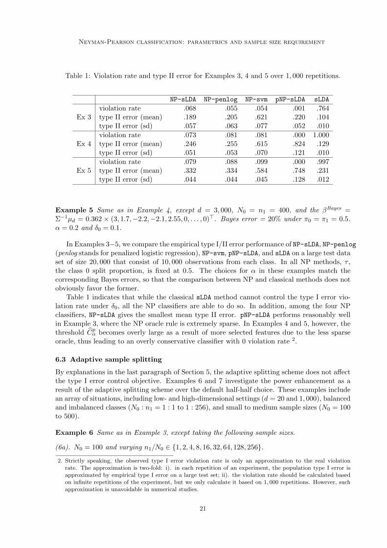
Table 1: Violation rate and type II error for Examples 3, 4 and 5 over 1, 000 repetitions.

NP-sLDA NP-penlog NP-svm pNP-sLDA sLDA

Ex 3violation rate .068 .055 .054 .001 .764type II error (mean) .189 .205 .621 .220 .104type II error (sd) .057 .063 .077 .052 .010

Ex 4violation rate .073 .081 .081 .000 1.000type II error (mean) .246 .255 .615 .824 .129type II error (sd) .051 .053 .070 .121 .010

Ex 5violation rate .079 .088 .099 .000 .997type II error (mean) .332 .334 .584 .748 .231type II error (sd) .044 .044 .045 .128 .012

Example 5 Same as in Example 4, except d = 3, 000, N0 = n1 = 400, and the βBayes =Σ−1µd = 0.362 × (3, 1.7,−2.2,−2.1, 2.55, 0, . . . , 0)>. Bayes error = 20% under π0 = π1 = 0.5.α = 0.2 and δ0 = 0.1.

In Examples 3−5, we compare the empirical type I/II error performance of NP-sLDA, NP-penlog(penlog stands for penalized logistic regression), NP-svm, pNP-sLDA, and sLDA on a large test dataset of size 20, 000 that consist of 10, 000 observations from each class. In all NP methods, τ ,the class 0 split proportion, is fixed at 0.5. The choices for α in these examples match thecorresponding Bayes errors, so that the comparison between NP and classical methods does notobviously favor the former.

Table 1 indicates that while the classical sLDA method cannot control the type I error vio-lation rate under δ0, all the NP classifiers are able to do so. In addition, among the four NPclassifiers, NP-sLDA gives the smallest mean type II error. pNP-sLDA performs reasonably wellin Example 3, where the NP oracle rule is extremely sparse. In Examples 4 and 5, however, thethreshold Cpα becomes overly large as a result of more selected features due to the less sparseoracle, thus leading to an overly conservative classifier with 0 violation rate 2.

6.3 Adaptive sample splitting

By explanations in the last paragraph of Section 5, the adaptive splitting scheme does not affectthe type I error control objective. Examples 6 and 7 investigate the power enhancement as aresult of the adaptive splitting scheme over the default half-half choice. These examples includean array of situations, including low- and high-dimensional settings (d = 20 and 1, 000), balancedand imbalanced classes (N0 : n1 = 1 : 1 to 1 : 256), and small to medium sample sizes (N0 = 100to 500).

Example 6 Same as in Example 3, except taking the following sample sizes.

(6a). N0 = 100 and varying n1/N0 ∈ {1, 2, 4, 8, 16, 32, 64, 128, 256}.

2. Strictly speaking, the observed type I error violation rate is only an approximation to the real violationrate. The approximation is two-fold: i). in each repetition of an experiment, the population type I error isapproximated by empirical type I error on a large test set; ii). the violation rate should be calculated basedon infinite repetitions of the experiment, but we only calculate it based on 1, 000 repetitions. However, suchapproximation is unavoidable in numerical studies.

21


(6b). Varying n1 = N0 ∈ {100, 150, 200, 250, 300, 350, 400, 450, 500}.

Example 7 Same as in Example 3, except that d = 20, N0 = 100 and varying n1/N0 ∈{1, 2, 4, 8, 16}.

Note that Examples 6a and 6b each includes 9 different simulation settings, and Example 7includes 5. For each simulation setting, we generate 1, 000 (training) datasets and a commontest set of size 100, 000 from class 1. Only class 1 test data are needed because only type IIerror is investigated in these examples. In each simulation setting, we train 10 NP classifiersof the same base algorithm using each of the 1, 000 datasets. Nine of these 10 NP classifiersuse fixed split proportions in {.1, · · · , .9}, and the last one uses adaptive split proportion usingK = 5. Overall in Examples 6 and 7, we set α = δ0 = 0.1, and train an enormous number of NPclassifiers. For instance, in Example 6a, we train 9 × 1, 000 × 10 = 90, 000 NP-sLDA classifiers,and the same number of NP classifiers for any other base algorithm under investigation. We fixthe thresholding rule as the NP umbrella algorithm in this subsection.

For each simulation setting, denote by R1(·) the empirical type II error on the test set. Wefix a simulation setting so that we do not need to have overly complex sub or sup indexes inthe following discussion. Denote by hi,b,τ an NP classifier with base algorithm b, trained on theith dataset (i ∈ {1, · · · , 1000}) using split proportion τ . This classifier also depends on users’choices of α and δ0, but we suppress these dependencies here to highlight our focus. In fixedproportion scenarios, τ ∈ {.1, · · · , .9}. Let τada(j, b) represent the adaptive split proportiontrained on the j-th dataset with base algorithm b using adaptive splitting scheme described inSection 5. Therefore, hi,b,τada(j,b) refers to the NP classifier with base algorithm b, trained on

the i-th dataset using the split proportion τada(j, b) pre-determined in the j-th dataset, wherei, j ∈ {1, · · · , 1000}. Let Aveb,τ and Aveb,τ be our performance measures for fix proportion andadaptive proportion respectively, which are defined by,

Aveb,τ =1

1000

1000∑i=1

R1(hi,b,τ ) , and Aveb,τ = medianj=1,··· ,1000

(1

1000

1000∑i=1

R1

(hi,b,τada(j,b)

)).

While the meaning of the measure Aveb,τ is almost self-evident, Aveb,τ deserves some elaboration.As we explained in the last paragraph of Section 5, the adaptive splitting scheme returns aproportion based on one realization of S, and then we adopt it in all subsequent realizations.Let

wb(j) =1

1000

1000∑i=1

R1

(hi,b,τada(j,b)

),

then wb(j) is a performance measure of the adaptive scheme if the proportion is returned fromtraining on the j-th dataset. To account for the variation among wb(j)’s for different choicesof j, we take the median over wb(j)’s as our final measure. Also, we denote the average ofadaptively selected proportions by τb,ada = 1

1000

∑1000j=1 τ

ada(j, b), and define the average optimalsplit proportion τb,opt by

τb,opt =1

1000

1000∑i=1

arg minτ∈{.1··· ,.9}

R1(hi,b,τ ) .

With Example 6, we investigate i). the effectiveness (in terms of type II error) of the adaptivesplitting strategy compared to a fixed half-half split, illustrated by the left panels of Figures 3

22


Figure 3: Example 6a. Left panel: type II error (Aveb,.5 and Aveb,τ ) of NP-sLDA and NP-penlog

vs. n1/N0; Right panel: average split proportion (τb,ada and τb,opt) vs. n1/N0. N0 is fixed to be100 for both panels.

●

●

●

●

●●

●● ●

●

●

●

●

●

● ●

●●

0.200

0.225

0.250

0.275

0.300

0.325

1 2 4 8 16 32 64 128 256

n1 N0

Type

II E

rror

●

●

penlog

sLDA

● 0.5

ada●

●

●

● ●

●

●

● ●

●

●

●

●

●

●

●

●

●

0.32

0.34

0.36

0.38

0.40

1 2 4 8 16 32 64 128 256

n1 N0

Ave

rage

Spl

it P

ropo

rtio

n

●

●

penlog

sLDA

● opt

ada

and 4; ii). how close is τb,ada compared to τb,opt, illustrated by the right panels of Figures 3and 4; iii). how the class imbalance affects NP-sLDA and NP-penlog, illustrated by both panelsof Figure 3; and iv). how the absolute class 0 sample size affects NP-sLDA and NP-penlog,illustrated by both panels of Figure 4.

In Figure 3 (Example 6a), the left panel presents the trend of type II errors (Aveb,.5 andAveb,τ ) as the sample size ratio n1/N0 increases from 1 to 256 for fixed N0 = 100. For bothNP-penlog and NP-sLDA, type II error decreases as n1/N0 increases from 1 to 16 and gradu-ally stabilizes afterwards. Neither NP-penlog nor NP-sLDA suffers from training on imbalancedclasses. In terms of type II error performance, the adaptive splitting strategy significantly im-proves over the fixed split proportion 0.5. The right panel of Figure 3 shows that, on averagethe adaptive split proportion is very close to the optimal one throughout all sample size ratios.

In Figure 4 (Example 6b), the left panel presents the trend of type II errors (Aveb,.5 andAveb,τ ) as the class 0 sample size N0 (n1 = N0) increases from 100 to 500, indicating that typeII error clearly benefits from increasing training sample sizes of both classes. For the same basealgorithm, the adaptive splitting strategy significantly improves over the fixed split proportion0.5 for N0 and n1 small, although the improvement diminishes as both sample sizes becomelarge. The right panel of Figure 4 shows that on average, the adaptive split proportion is veryclose to the optimal one throughout all sample sizes. Furthermore, the average optimal splitproportion seems to increase as N0 increases in general. An intuition is that when N0 is smaller,a higher proportion of class 0 observations is needed for threshold estimate, to guarantee thetype I error violation rate control.

With Example 7, we investigate the interaction between adaptive splitting strategy andmultiple random splits on different NP classifiers. Multiple random splits of class 0 observationswere proposed in the NP umbrella algorithm in Tong et al. (2018) to increase the stability ofthe type II error performance. When an NP classifier uses M > 1 multiple splits, each split willresult in a classifier, and the final prediction rule is a majority vote of these classifiers. Figure5 shows the trend of type II error of NP-sLDA, NP-penlog, NP-randomforest, and NP-svm, asthe sample size ratio n1/N0 increases from 1 to 16 while keeping N0 = 100. For each base

23


Figure 4: Example 6b. Left panel: type II error (Aveb,.5 and Aveb,τ ) of NP-sLDA and NP-penlog

vs. N0; Right panel: average split proportion (τb,ada and τb,opt) vs. N0. n1 = N0 for both panels.

●

●

●

●

●

●●

●●

●

●

●

●

●

●

●

●●

0.15

0.20

0.25

0.30

100 200 300 400 500

N0

Type

II E

rror

●

●

penlog

sLDA

● 0.5

ada

● ●

●

●

●

●

●

●●

●

●

●

●

●

●

●

●

●

0.350

0.375

0.400

0.425

0.450

100 200 300 400 500

N0

Ave

rage

Spl

it P

ropo

rtio

n

●

●

penlog

sLDA

● opt

ada

Figure 5: Example 7. Type II error (Aveb,.5 and Aveb,τ ) vs. sample size ratios for four NPclassifiers (NP-sLDA, NP-penlog, NP-svm, NP-randomforest), with both multiple random splits(M = 11) and single random split. N0 = 100 for all sample size ratios.

●● ● ● ●

●● ● ● ●

●

●

●

●

●

●

●

●

●

●

●● ● ● ●

●●

● ●●

●

●

●

●

●

●●

●

●

●

0.2

0.3

0.4

0.5

0.6

4 8 12 16

n1 N0

Med

ian

Type

II E

rror

multi

single

● 0.5

ada

●

●

●

●

penlog

randomforest

sLDA

svm

24


Table 2: Example 7. Average computational cost (in seconds) for four NP-classifiers (NP-sLDA,NP-penlog, NP-randomforest, NP-svm) over 1,000 repetitions (standard deviation in parenthe-ses).

n1/N0 NP-sLDA NP-penlog NP-randomforest NP-svm

1 1.17(0.14) 3.58(0.58) 1.49(4.83) 33.81(2.08)2 1.19(0.13) 5.24(1.03) 1.43(0.16) 36.09(1.98)4 1.19(0.14) 7.63(1.79) 2.06(0.10) 41.44(2.38)8 1.22(0.09) 11.11(2.31) 3.43(0.19) 53.25(6.21)16 1.30(0.08) 16.08(3.79) 6.92(0.25) 84.64(5.28)

algorithm, four scenarios are considered: (fixed 0.5 split proportion, single split), (adaptivesplit proportion, single split), (fixed 0.5 split proportion, multiple splits), and (adaptive splitproportion, multiple splits). Figure 5 suggests the following interesting findings: i). type IIerror decreases for NP-sLDA and NP-penlog but increases for NP-randomforest and NP-svm, asa function of n1/N0 while keeping N0 constant; ii). with both fixed 0.5 split proportion andadaptive splitting strategy, performing multiple splits leads to a smaller type II error comparedwith their single split counterparts; iii). for both single split and multiple splits, the adaptivesplit always improves upon the fixed 0.5 split proportion; iv). NP-svm and NP-randomforest

are affected by the imbalance scenario, and one might consider downsampling or upsamplingmethods before applying an NP algorithm; and v). adding multiple splits to the adaptivesplitting strategy leads to a further reduction on the type II error. Nevertheless, the reductionin type II error from the adaptive splitting scheme alone is much larger than the marginal gainfrom adding multiple splits on top of it. Therefore, when computation power is limited, oneshould implement the adaptive splitting scheme before considering multiple splits.

Lastly, from Table 2, we would like to point out NP-sLDA is the fastest method to computeamong the four NP classifiers with more evident advantages as the sample size increases. 3

6.4 Real data analysis

We study two high-dimensional datasets in this subsection. The first is a neuroblastoma datasetcontaining d = 43, 827 gene expression measurements from N = 498 neuroblastoma samplesgenerated by the Sequencing Quality Control (SEQC) consortium (Wang et al., 2014). Thesamples fall into two classes: 176 high-risk (HR) samples and 322 non-HR samples. It is usuallyunderstood that misclassifying an HR sample as non-HR will have more severe consequencesthan the other way around. Formulating this problem under the NP classification framework, welabel the HR samples as class 0 observations and the non-HR samples as class 1 observations and,use all gene expression measurements as features to perform classification. We set α = δ0 = 0.1,and compare NP-sLDA with NP-penlog, NP-randomforest and NP-svm. We randomly split thedataset 1, 000 times into a training set (70%) and a test set (30%), and then train the NPclassifiers on each training data and compute their empirical type I and type II errors over thecorresponding test data. We consider each fixed split proportion in {.1, .2, .3, .4, .5, .6, .7, .8} aswell as the adaptive splitting strategy. Here, the split proportion 0.9 is not considered since it

3. All numerical experiments were performed on HP Enterprise XL170r with CPU E5-2650v4 (2.20 GHz) and16 GB memory.

25


Figure 6: The average type I and type II errors vs. splitting proportion on the neuroblastomadata set for NP-sLDA, NP-penlog, NP-randomforest and NP-svm over 1, 000 random splits. The“*” point on each line represents the average split proportion chosen by adapting splitting.

●

●

●

●

●

●

●

●

****

0.04

0.05

0.06

0.2 0.4 0.6 0.8

Split Proportion

Type

I E

rror

● penlog

randomforest

sLDA

svm

●

●

●

●

●

●

●

●

**

*

*

0.075

0.100

0.125

0.150

0.175

0.200

0.2 0.4 0.6 0.8

Split Proportion

Type

II E

rror

● penlog

randomforest

sLDA

svm

leads to a left-out sample size which is too small to control the type I error at the given α andδ0 values. Figure 6 indicates that the average type I error is less than α across different splitproportions for all four methods considered. Regarding the average type II error, NP-sLDA hasthe smallest values for a wide range of split proportions. In particular, the smallest averagetype II error for NP-sLDA corresponds to split proportion 0.4. The average location of the splitproportion chosen by the adaptive splitting scheme would lead to a type II error close to theminimum. This demonstrates that the adaptive splitting scheme works well for different NPclassifiers. Lastly, we note that for a specific splitting proportion, the median computation timeis 213.95 seconds for pNP-sLDA vs. 1717.69 seconds for NP-randomforest over 1,000 randomsplits.

The second dataset is a high-dimensional breast cancer dataset (d = 22, 215, N = 118)(Chin et al., 2006) with gene expression measurements of subjects that fall into positive (class0, N = 75) and negative (class 1, n1 = 43) groups. We set δ0 = 0.1 and vary α from 0.05 to0.15, and compare the performance of NP-sLDA with pNP-sLDA. We randomly split the dataset1,000 times into a training set (2/3) and a test set (1/3), train the two methods on the trainingset, and compute the empirical type I and type II errors on the corresponding test set. Due tothe limited sample size, it is clear from Table 3 that when α is small, the minimum sample sizerequirement for the NP umbrella algorithm is not satisfied. The pNP-sLDA, on the other hand,took advantage of the parametric assumption and the corresponding violation rate is under δ0

throughout all choices of α.

7. Discussion

This work develops Neyman-Pearson (NP) classification theory and methodology under para-metric model assumptions. Most specifically, based on the linear discriminant analysis (LDA)model, we develop a new parametric model-based thresholding rule for high probability type Ierror control, and this complements the nonparametric NP umbrella algorithm when the mini-mum sample size requirement of the latter is not met. In practice, when the minimum sample

26


Table 3: Violation rate and average type II errors over 1,000 replications for the breast cancerdata. Here, δ0 = 0.1 and α varies from 0.05 to 0.15.

α vio (NP) vio (pNP) type II (NP) type II (pNP)

0.05 NA 0.021 NA 0.6630.06 NA 0.025 NA 0.6260.07 NA 0.029 NA 0.5940.08 NA 0.015 NA 0.5650.09 0.111 0.015 0.448 0.5360.1 0.111 0.015 0.448 0.515

size requirement is met and the scoring function depends on more than a few features, the NPumbrella algorithm is still recommended based on better empirical performance. For futurework, it would be interesting to investigate NP classifiers under other parametric settings, suchas quadratic discriminant analysis (QDA) model and heavy-tailed distributions which are ap-propriate to model financial data. We expect that new model-specific thresholding rules will bedeveloped for NP classification.

Acknowledgement

The authors would like to thank the Action Editor and three anonymous referees for manyconstructive comments which greatly improved the paper. This work was partially supportedby National Science Foundation grants DMS-1554804 and DMS-1613338, and National Institutesof Health grant R01 GM120507.

Appendix A. Neyman-Pearson Lemma

The oracle classifier under the NP paradigm arises from its close connection to the Neyman-Pearson Lemma in statistical hypothesis testing. Hypothesis testing bears strong resemblance tobinary classification if we assume the following model. Let P1 and P0 be two known probabilitydistributions on X ⊂ Rd. Assume that Y ∼ Bern(ζ) for some ζ ∈ (0, 1), and the conditionaldistribution of X given Y is PY . Given such a model, the goal of statistical hypothesis testingis to determine if we should reject the null hypothesis that X was generated from P0. To thisend, we construct a randomized test φ : X → [0, 1] that rejects the null with probability φ(X).Two types of errors arise: type I error occurs when P0 is rejected yet X ∼ P0, and type IIerror occurs when P0 is not rejected yet X ∼ P1. The Neyman-Pearson paradigm in hypothesistesting amounts to choosing φ that solves the following constrained optimization problem

maximize IE[φ(X)|Y = 1] , subject to IE[φ(X)|Y = 0] ≤ α ,

where α ∈ (0, 1) is the significance level of the test. A solution to this constrained optimizationproblem is called a most powerful test of level α. The Neyman-Pearson Lemma gives mildsufficient conditions for the existence of such a test.

Lemma 16 (Neyman-Pearson Lemma) Let P1 and P0 be two probability measures with den-sities f1 and f0 respectively, and denote the density ratio as r(x) = f1(x)/f0(x). For a given

27


significance level α, let Cα be such that P0{r(X) > Cα} ≤ α and P0{r(X) ≥ Cα} ≥ α. Then,the most powerful test of level α is

φ∗α(X) =

1 if r(X) > Cα ,0 if r(X) < Cα ,α−P0{r(X)>Cα}P0{r(X)=Cα} if r(X) = Cα .

Under mild continuity assumption, we take the NP oracle classifier

φ∗α(x) = 1I{f1(x)/f0(x) > Cα} = 1I{r(x) > Cα} , (22)

as our plug-in target for NP classification.

Appendix B. Additional Lemmas and Propositions

Lemma 17 (Hsu et al. (2012)) Let A ∈ Rm×n be a matrix, and let Σ := A>A. Let x =(x1, · · · , xn)> be an isotropic multivariate Gaussian random vector with mean zero. For allt > 0,

IP(‖Ax‖2 > tr(Σ) + 2

√tr(Σ2)t+ 2‖Σ‖t

)≤ e−t .

Lemma 18 Recall that βBayes = Σ−1µd = Σ−1(µ1−µ0) and A = {j : {Σ−1µd}j 6= 0}. Denote by

β∗ = (ΣAA)−1(µ1A−µ0

A) and βBayes by letting βBayesA = β∗ and βBayes

Ac = 0. Then βBayes = βBayes.

Recall these notations for the following lemma: let S0 = {x01, · · · , x0

n0} be an i.i.d. sample of

class 0 of size n0 and S1 = {x11, · · · , x1

n1} be an i.i.d. sample of class 1 of size n1, and n = n0 +n1.

We use S0 and S1 to find an estimate of βBayes. Let X be the (n× d) centered predictor matrix,whose column-wise mean is zero, which can be decomposed into X0, the (n0 × d) centeredpredictor matrix based on class 0 observations and X1, the (n1 × d) centered predictor matrixbased on class 1 observations. Let C(n) = (X)>X/n, then

C(n) =n0

nΣ0 +

n1

nΣ1 ,

where Σ0 = (X0)T X0/n0 , and Σ1 = (X1)T X1/n1 .

Lemma 19 Suppose there exists c > 0 such that Σjj ≤ c for all j = 1, · · · , d. There existconstants ε0 and c1, c2 such that for any ε ≤ ε0 we have,

IP(|(µ1

j − µ0j )− (µ1

j − µ0j )| ≥ ε)

)≤ 2 exp(−n0ε

2c2) + 2 exp(−n1ε2c2) , for j = 1, · · · , d . (23)

IP(|Σlij − Σij | ≥ ε

)≤ 2 exp(−nlε2c1) , for l = 0, 1, i, j = 1, · · · , d . (24)

IP(‖Σl

AA − ΣAA‖∞ ≥ ε)≤ 2s2 exp(−nls−2ε2c1) . (25)

IP(‖ΣAcA − ΣAcA‖∞ ≥ ε

)≤ (d− s)s exp(−nls−2ε2c1) . (26)

IP(‖(µ1 − µ0)− (µ1 − µ0)‖∞ ≥ ε

)≤ 2d exp(−n0ε

2c2) + 2d exp(−n1ε2c2) . (27)

28


IP(‖(µ1

A − µ0A)− (µ1

A − µ0A)‖∞ ≥ ε

)≤ 2s exp(−n0ε

2c2) + 2s exp(−n1ε2c2) . (28)

IP(|C(n)ij − Σij | ≥ ε

)≤ 2 exp

(−c1ε

2n2

4n0

)+ 2 exp

(−c1ε

2n2

4n1

). (29)

IP(|C(n)AA − ΣAA| ≥ ε

)≤ 2s2 exp

(−c1ε

2n2

4s2n0

)+ 2s2 exp

(−c1ε

2n2

4s2n1

). (30)

IP(|C(n)AcA − ΣAcA| ≥ ε

)≤ (d− s)s exp

(−c1ε

2n2

4s2n0

)+ (d− s)s exp

(−c1ε

2n2

4s2n1

). (31)

Lemma 20 Recall that κ = ‖ΣAcA(ΣAA)−1‖∞, ϕ = ‖(ΣAA)−1‖∞ and ∆ = ‖µ1A − µ0

A‖∞. Let

C(n)AcA = n0

n (X0Ac)>X0

A + n1n (X1

Ac)>X1

A = n0n Σ0

AcA + n1n Σ1

AcA, and C(n)AA = n0

n Σ0AA + n1

n Σ1AA. There

exist constants c1 and ε0 such that for any ε ≤ min(ε0, 1/ϕ), we have

IP(‖C(n)

AcA(C(n)AA)−1 − ΣAcA(ΣAA)−1‖∞ ≥ (κ+ 1)εϕ(1− ϕε)−1

)≤ f(d, s, n0, n1, ε) ,

where f(d, s, n0, n1, ε) = (d+ s)s exp(− c1ε2n2

4s2n0

)+ (d+ s)s exp

(− c1ε2n2

4s2n1

), and n = n0 + n1.

Lemma 21 Let C0 be in Equation (39), C as in Lemma 10, and XA = Σ−1/2AA XA. Assume

λm = λmin(Σ−1/2AA ) is bounded from below, then we have

P0{C∗∗α ≤ s∗(X) ≤ C∗∗α + δ|X ∈ C} ≥ (1− δ3)P0(C∗∗α ≤ (µ1A − µ0

A)>Σ−1/2AA XA ≤ C∗∗α + δ|C0) ,

where δ3 = exp{−(n0 ∧ n1)1/2}.

Lemma 22 Let us denote a = Σ−1/2AA (µ1

A − µ0A). Assume there exist M > 0 such that the

following conditions hold:

i) C∗∗α − (µ1A − µ0

A)>Σ−1AAµ

0A ∈ (C1, C2) for some constants C1, C2.

ii) When s = 1, a is a scalar. fN (0,|a|) is bounded below on interval (C1, C2 + δ∗) by M .

iii) When s = 2, a = (a1, a2)> is a vector. 1√

2π|a1|(a2

2

a21

+ 1) exp{−a

21 + a2

2 − a22a

21

a21(a2

1 + a22)

t2}

(2Φ(

√L2 − a2

1 + a22 − a2

2a21

a21(a2

1 + a22)

t2)− 1

)

is bounded below on interval t ∈ (C1, C2 + δ∗) by M .

Then, for s ≤ 2, for any δ ∈ (0, δ∗), there exists M1 which is a constant depending on M , suchthat the following inequality holds

P0(C∗∗α ≤ (µ1A − µ0

A)>Σ−1/2AA XA ≤ C∗∗α + δ|C0) ≥M1δ.

Proposition 23 Suppose that λmin(Σ−1/2AA ), the minimum eigenvalue of Σ

−1/2AA , is bounded from

below. Let us denote a = Σ−1/2AA (µ1

A−µ0A). Let us also assume that there exists M > 0 such that

the following conditions hold:

29


i) C∗∗α − (µ1A − µ0

A)>Σ−1AAµ

0A ∈ (C1, C2) for some constants C1, C2.

ii) When s = 1, a is a scalar. fN (0,|a|) is bounded below on interval (C1 − δ∗, C2 + δ∗) by M .

iii) Let L = λmin(Σ−1/2AA )c′1s

1/2(n0 ∧ n1)1/4. When s = 2, a = (a1, a2) is a vector. 1√

2π|a1|(a2

2

a21

+ 1) exp{−a

21 + a2

2 − a22a

21

a21(a2

1 + a22)

t2}

(2Φ(

√L2 − a2

1 + a22 − a2

2a21

a21(a2

1 + a22)

t2)− 1

)

is bounded below on interval t ∈ (C1 − δ∗, C2 + δ∗) by M .

Then for s ≤ 2, the function s∗(·) satisfies conditional detection condition restricted to C oforder γ

−= 1 with respect to P0 at the level (C∗∗α , δ

∗). In other words, Assumption 2 is satisfied.

Appendix C. Simulation for the control of largest empirical eigenvalues

Here, we present a simulation to verify the inequality on the largest eigenvalue of the samplecovariance matrix in relation to that of the population covariance matrix, as stated in (17).

Example 8 The data are generated from an LDA model with common covariance matrix Σ.We set ε = 1e − 3 and consider the 8 combinations for the following three factors and varyN0 = n1 ∈ {20, 40, 60, 80, 100, 120, 140, 160, 180, 200}. µ0 = 0d.

(8a). The dimension d ∈ {3, 10}. µ1 = 1.16 · 13 when d = 3 and µ1 = 0.75 · 110 when d = 10.

(8b). Σ is set to be an AR(1) covariance matrix with Σij = ρ|i−j| or an CS (compound symmetry)covariance matrix with Σii = 1 and Σij = ρ for all i 6= j.

(8c). The correlation parameter ρ ∈ {.5, .9}.

From Table 4, it is clear that the bound is satisfied with very high probability across all scenariosconsidered.

Table 4: The probability that the bound stated in (17) is satisfied over 1000 replications.

Covarianceρ

N0 20 40 60 80 100 120 140 160 180 200

d = 3AR(1)

.5 1.0 1.0 1.0 1.0 1.0 .999 .999 1.0 .999 1.0

.9 1.0 1.0 1.0 1.0 1.0 .999 .999 1.0 .999 1.0

CS.5 1.0 1.0 1.0 1.0 1.0 1.0 1.0 1.0 1.0 1.0.9 1.0 1.0 1.0 1.0 1.0 1.0 1.0 1.0 1.0 1.0

d = 10AR(1)

.5 1.0 1.0 1.0 1.0 1.0 1.0 1.0 1.0 1.0 1.0

.9 1.0 1.0 1.0 1.0 1.0 1.0 1.0 1.0 1.0 1.0

CS.5 1.0 1.0 1.0 1.0 1.0 1.0 1.0 1.0 1.0 1.0.9 1.0 1.0 1.0 1.0 1.0 1.0 1.0 1.0 1.0 1.0

30


Appendix D. Proofs

Proof [Proof of Lemma 8] By Corollary 6, k∗ ≤ k′. This implies that R0(φk∗) ≥ R0(φk′).Moreover, by Lemma 7, for any δ′0 ∈ (0, 1) and n′0 ≥ 4/(αδ0),

IP(|R0(φk′)−R0(φ∗α)| > ξα,δ0,n′0(δ′0)

)≤ δ′0 .

Let E0 = {R0(φk∗) ≤ α} and E1 = {|R0(φk′)−R0(φ∗α)| ≤ ξα,δ0,n′0(δ′0)}. On the event E0 ∩ E1, wehave

α = R0(φ∗α) ≥ R0(φk∗) ≥ R0(φk′) ≥ R0(φ∗α)− ξα,δ0,n′0(δ′0) ,

This implies that

|R0(φk∗)−R0(φ∗α)| ≤ ξα,δ0,n′0(δ′0) .

Proof [Proof of Lemma 10] Note that Σ−1/2AA (XA−µ0

A) ∼ N (0, Is). By Lemma 17, for all t > 0,

P0

(‖XA − µ0

A‖2 > tr(ΣAA) + 2√tr(Σ2

AA)t+ 2‖ΣAA‖t)≤ e−t .

For t = (n0 ∧ n1)1/2 (> 1), the above inequality implies there exists some c′′1 > 0 such that

P0(‖XA − µ0A‖2 > c′′1st) ≤ e−t .

Similarly, P1(‖XA − µ1A‖2 > c′′1st) ≤ e−t. Let C0 = {X : ‖XA − µ0

A‖2 ≤ c′′1st} and C1 ={X : ‖XA − µ1

A‖2 ≤ c′′1st}. There exists some c′1 > 0, such that both C0 and C1 are subsetsof C = {X : ‖XA‖ ≤ c′1s

1/2t1/2}. Then P0(X ∈ C) ≥ 1 − δ3 and P1(X ∈ C) ≥ 1 − δ3, forδ3 = exp{−(n0 ∧ n1)−1/2}.

By Proposition 9, for δ1 ≥ δ∗1 and δ2 ≥ δ∗2 , we have with probability at least 1 − δ1 − δ2,

βlassoAc = βBayes

Ac = 0. Moreover,

‖s− s∗‖∞,C ≤ maxx∈C|x>Aβlasso

A − x>AβBayesA |+ max

x∈C|x>Ac βlasso

Ac − x>AcβBayesAc |

= maxx∈C|x>Aβlasso

A − x>AβBayesA |

≤ ‖βlassoA − βBayes

A ‖∞ ·maxx∈C‖XA‖1

≤ ‖βlassoA − βBayes

A ‖∞ ·√smaxx∈C‖XA‖2

≤ 4ϕλ · c′1s(n0 ∧ n1)1/4 ,

where the last inequality uses a relation β∗ = βBayesA , which is derived in Lemma 18.

Proof [Proof of Lemma 11] Note that by Lemma 10, P0(X ∈ C) ≥ 1− exp{−(n0 ∧ n1)1/2}, sowe have

|R0(φk∗)−R0(φ∗α)|= |[R0(φk∗ |C)−R0(φ∗α|C)]P0(X ∈ C) + [R0(φk∗ |Cc)−R0(φ∗α|Cc)]P0(X ∈ Cc)|≥ |[R0(φk∗ |C)−R0(φ∗α|C)]P0(X ∈ C)| − |[R0(φk∗ |Cc)−R0(φ∗α|Cc)]P0(X ∈ Cc)|≥ |R0(φk∗ |C)−R0(φ∗α|C)|(1− exp{−(n0 ∧ n1)1/2})− 1 · exp{−(n0 ∧ n1)1/2} .

31


Lemma 8 says that

IP{|R0(φk∗)−R0(φ∗α)| > ξα,δ0,n′0(δ′0)} ≤ δ0 + δ′0 .

This combined with the above inequality chain implies

IP{|R0(φk∗ |C)−R0(φ∗α|C)| >[ξα,δ0,n′0(δ′0) + exp{−(n0 ∧ n1)1/2}]

1− exp{−(n0 ∧ n1)1/2}} ≤ δ0 + δ′0 .

Since exp{−(n0 ∧ n1)1/2} ≤ 1/2, the conclusion follows.

Proof [Proof of Lemma 18] Note that µ1 − µ0 = ΣβBayes. After shuffling the A coordinates tothe front if necessary, we have

µ1 − µ0 =

[ΣAA ΣAAc

ΣAcA ΣAcAc

][βBayesA

βBayesAc

].

Then, µ1A − µ0

A = (ΣAA)βBayesA as βBayes

Ac = 0 ∈ R|Ac| by definition. Therefore we have,

β∗ = Σ−1AA(µ1

A − µ0A) = βBayes

A ,

which combined with βBayesAc = βBayes

Ac = 0 leads to βBayes = βBayes.

Proof [Proof of Lemma 19]Inequalities (23)-(28) can be proved similarly as in Mai et al. (2012), so proof is omitted.Inequalities (29)-(31) can be proved by applying (24)-(26) respectively and observe that

A + B ≥ ε implies A ≥ ε/2 or B ≥ ε/2. More concretely, they are proven by the followingarguments:

IP(|C(n)ij − Σij | ≥ ε

)= IP

(|n0

nΣ0ij +

n1

nΣ1ij − Σij | ≥ ε

)≤ IP

(n0

n|Σ0ij − Σij | ≥ ε/2

)+ IP

(n1

n|Σ1ij − Σij | ≥ ε/2

)= IP

(|Σ0ij − Σij | ≥

nε

2n0

)+ IP

(|Σ1ij − Σij | ≥

nε

2n1

)≤ 2 exp

(−c1ε

2n2

4n0

)+ 2 exp

(−c1ε

2n2

4n1

).

IP(|C(n)AA − ΣAA| ≥ ε

)= IP

(|n0

nΣ0AA +

n1

nΣ1AA − ΣAA| ≥ ε

)≤ IP

(n0

n|Σ0AA − ΣAA| ≥ ε/2

)+ IP

(n1

n|Σ1AA − ΣAA| ≥ ε/2

)≤ 2s2 exp

(−c1ε

2n2

4n0s2

)+ 2s2 exp

(−c1ε

2n2

4n1s2

).

IP(|C(n)AcA − ΣAcA| ≥ ε

)= IP

(|n0

nΣ0AcA +

n1

nΣ1AcA − ΣAcA| ≥ ε

)≤ IP

(n0

n|Σ0AcA − ΣAcA| ≥ ε/2

)+ IP

(n1

n|Σ1AcA − ΣAcA| ≥ ε/2

)≤ (d− s)s exp

(−c1n

2ε2

4s2n0

)+ (d− s)s exp

(−c1n

2ε2

4s2n1

).

32


Proof [Proof of Lemma 20] Let η1 = ‖ΣAA − C(n)AA‖∞, η2 = ‖ΣAcA − C

(n)AcA‖∞, and η3 =

‖(C(n)AA)−1 − (ΣAA)−1‖∞.

‖C(n)AcA(C

(n)AA)−1 − ΣAcA(ΣAA)−1‖∞ ≤ ‖C(n)

AcA − ΣAcA‖∞ × ‖(C(n)AA)−1 − (ΣAA)−1‖∞

+‖C(n)AcA − ΣAcA‖∞ × ‖(ΣAA)−1‖∞

+‖ΣAcA(ΣAA)−1‖∞ × ‖ΣAA − C(n)AA‖∞ × ‖(ΣAA)−1‖∞

+‖ΣAcA(ΣAA)−1‖∞ × ‖ΣAA − C(n)AA‖∞

×‖(C(n)AA)−1 − (ΣAA)−1‖∞

≤ (κη1 + η2)(ϕ+ η3) .

Moreover, η3 ≤ ‖(C(n)AA)−1‖∞×‖C(n)

AA−ΣAA‖∞×‖(ΣAA)−1‖∞ ≤ (ϕ+η3)ϕη1. Hence, if ϕη1 < 1,we have η3 ≤ ϕ2η1(1− ϕη1)−1. Hence we have,

‖C(n)AcA(C

(n)AA)−1 − ΣAcA(ΣAA)−1‖∞ ≤ (κη1 + η2)ϕ(1− ϕη1)−1 .

Then we consider the event max(η1, η2) ≤ ε. Note that ε < 1/ϕ ensures that ϕη1 < 1 on thisevent. The conclusion follows from inequalities (30) and (31).

Proof [Proof of Lemma 21] Since (Σ−1µd)A = Σ−1AA(µ1

A−µ0A) (by Lemma 18) and C0 ⊂ C0 ⊂ C,

we have

P0{C∗∗α ≤ s∗(X) ≤ C∗∗α + δ|X ∈ C}≥ P0({C∗∗α ≤ (µ1

A − µ0A)>Σ−1

AAXA ≤ C∗∗α + δ} ∩ C)

≥ P0({C∗∗α ≤ (µ1A − µ0

A)>Σ−1AAXA ≤ C∗∗α + δ} ∩ C0)

= P0({C∗∗α ≤ (µ1A − µ0

A)>Σ−1/2AA XA ≤ C∗∗α + δ}|C0)P0(C0)

≥ (1− δ3)P0(C∗∗α ≤ (µ1A − µ0

A)>Σ−1/2AA XA ≤ C∗∗α + δ|C0) ,

where the last inequality uses P0(C0) ≥ 1− δ3. To derive this inequality, let V 0 (defined in theproof of Proposition 23) play the role of x and take A = Is in Lemma 17, then we have

IP(‖V 0‖2 ≥ s+ 2

√st+ 1 · t

)≤ e−t , for all t > 0 .

For s, t ∈ N, the above inequality clearly implies IP(‖V 0‖2 ≥ 4st) ≤ exp(−t). Take t = (n0 ∧n1)1/2, then as long as c′1 ≥ 2/λm,

{x : ‖V 0‖2 ≤ 4st} ⊂ {x : ‖V 0‖2 ≤ λ2m(c′1)2st} = C0 .

Since λm is bounded from below, we can certainly take c′1 ≥ 2/λm is the proof of Lemma

10 in constructing C0. Therefore, IP(‖V 0‖2 ≤ s + 2√st + t) ≥ 1 − exp(−t) implies that

IP(C0) ≥ 1− exp(−t) for t = (n0 ∧ n1)1/2.

33


Proof [Proof of Lemma 22] Since V 0 = XA − Σ−1/2AA µ0

A, it follows that,

P0(C∗∗α ≤ (µ1A − µ0

A)>Σ−1/2AA XA ≤ C∗∗α + δ|C0)

=P0(C∗∗α − (µ1A − µ0

A)>Σ−1AAµ

0A ≤ a>V 0 ≤ C∗∗α + δ − (µ1

A − µ0A)>Σ−1

AAµ0A|C0).

By Mukerjee and Ong (2015), the probability density function of V 0|C0 is given by

fV 0|C0(v) =

{kL,s

Πsi=1φ(vi) if ‖v‖ ≤ L

0 , otherwise,(32)

where φ is the pdf for the standard normal random variable, L is defined in equation (39), andkL,s

is a normalizing constant. Note that kL,s

is a monotone decreasing function of L for each s,

and when L goes to infinity, kL,s

= k0s is a positive constant. Therefore, k

L,sis bounded below

by k0s . Since we only consider s ∈ {1, 2}, we can take k0 as a universal constant independent of

s, and kL,s

is bounded below by k0 universally.

Let fa>V 0|C0(z) be the density of a>V 0|C0. Thus, we want to lower bound

P0(C∗∗α − (µ1A − µ0

A)>Σ−1AAµ

0A ≤ a>V 0 ≤ C∗∗α + δ − (µ1

A − µ0A)>Σ−1

AAµ0A|C0)

=

∫ C∗∗α +δ−(µ1A−µ

0A)>Σ−1

AAµ0A

C∗∗α −(µ1A−µ

0A)>Σ−1

AAµ0A

fa>V 0|C0(z)dz .

Let us analyze fa>V 0|C0(z) when s = 1 and s = 2.

Case 1 (s = 1): a is a scalar. Hence

faV 0|C0(z) =

{kL,1

|a| φ( za), for |z| ≤ |a|L0, otherwise,

which is the density function of a truncated Normal random variable with parent distributionN (0, |a|) symmetrically truncated to −|a|L and |a|L, i.e. TN(0, |a|,−|a|L, |a|L). Here |a| is thestandard deviation of the parent Normal distribution. Therefore,

faV 0|C0(z) ≥ fN (0,|a|)(z), for |z| ≤ |a|L.

This implies∫ C∗∗α +δ−(µ1A−µ

0A)>Σ−1

AAµ0A


0A)>Σ−1

AAµ0A

faV 0|C0(z)dz

≥ δmin{fN (0,|a|)(C∗∗α − (µ1

A − µ0A)>Σ−1

AAµ0A), fN (0,|a|)(C

∗∗α − (µ1

A − µ0A)>Σ−1

AAµ0A + δ∗)}

≥ δM.

where the inequality follows from the mean-value theorem and our assumption (ii).Case 2 (s = 2): a = (a1, a2) is a vector. Now let us do the following change of variable from(V1, V2) = V 0|C to (Z1, Z2) = (a>V 0|C, V2).{

Z1 = a1V1 + a2V2

Z2 = V2

, and thus

{V1 = Z1−a2Z2

a1

V2 = Z2

(33)

34


The original event SV1,V2 = {V 21 + V 2

2 ≤ L2} is equivalent to

SZ1,Z2 =

(Z1 − a2Z2

a1

)2

+ Z22 ≤ L2

⇔(a2

2

a21

+ 1

)(Z2 −

(a1a2

a21 + a2

2

)Z1

)2

+a2

1 + a22 − a2

1a22

a21(a2

1 + a22)

Z21 ≤ L2.

Now for any z1, the marginal density of a>V 0 can be carried out as

fZ1(z1)

=

∫Sz1,z2

kL,2

|a1|φ

(z1 − a2z2

a1

)φ(z2)dz2

=

∫Sz1,z2

kL,2

2π|a1|exp{−1

2

(z1 − a2z2

a1

)2

− z22

2}dz2

=

(kL,2

2π|a1|exp{−a

21 + a2

2 − a22a

21

2a21(a2

1 + a22)

z21}

)∫Sz1,z2

exp{−(z2 −

(a1a2

a21+a2

2

)z1)2

2a2

2/a21+1

}dz2

=

kL,2

|a1|√

2π(a2

2

a21

+ 1)

exp{−a21 + a2

2 − a22a

21

2a21(a2

1 + a22)

z21}

∫Sz1,z2

φN ((a1a2a21+a2

2

)z1,

1√a22/a

21+1

)(z2)dz2

=

kL,2

√2π|a1|

(a22

a21

+ 1) exp{−a

21 + a2

2 − a22a

21

a21(a2

1 + a22)

z21}

∫√L2−

a21+a2

2−a22a

21

a21(a2

1+a22)

z21

−

√L2−

a21+a2

2−a22a

21

a21(a2

1+a22)

z21

φN (0,1)(z)dz

=

kL,2

√2π|a1|

(a22

a21

+ 1) exp{−a

21 + a2

2 − a22a

21

a21(a2

1 + a22)

z21}

(2Φ(

√L2 − a2

1 + a22 − a2

2a21

a21(a2

1 + a22)

z21)− 1

).

This implies∫ C∗∗α +δ−(µ1A−µ

0A)>Σ−1

AAµ0A


0A)>Σ−1

AAµ0A

fa>V 0|C0(z)dz

≥ δmin{fZ1(C∗∗α − (µ1A − µ0

A)>Σ−1AAµ

0A), fZ1(C∗∗α − (µ1

A − µ0A)>Σ−1

AAµ0A + δ∗)}

≥ δMk0.

where the inequality follows from the mean-value theorem and our assumption (iii).

We can safely conclude our proof by combining cases s = 1 and s = 2, and taking M1 =min{M,Mk0}.

Proof [Proof of Proposition 9] The proof is largely identical to that of Theorem 1 in Mai et al.(2012), except the differences due to a different sampling scheme.

35


Similarly to Mai et al. (2012), by the definition of βA, we can write βA = (n−1X>A XA)−1{(µ1A−

µ0A) − λtA/2}, where tA represents the subgradient such that tj = sign(βj) if βj 6= 0 and

−1 < tj < 1 if βj = 0. To show that βlasso = (βA, 0), it suffices to verify that

‖n−1X>AcXAβA − (µ1Ac − µ0

Ac)‖∞ ≤ λ/2 . (34)

The left-hand side of (34) is equal to

‖C(n)AcA(C

(n)AA)−1(µ1

A − µ0A)− C(n)

AcA(C(n)AA)−1λtA/2− (µ1

Ac − µ0Ac)‖∞. (35)

Using ΣAcAΣ−1AA(µ1

A − µ0A) = (µ1

Ac − µ0Ac), (35) is bounded from above by

U1 = ‖C(n)AcA(C

(n)AA)−1 − ΣAcAΣ−1

AA‖∞∆ + ‖(µ1Ac − µ0

Ac)− (µ1Ac − µ0

Ac)‖∞+(‖C(n)

AcA(C(n)AA)−1 − ΣAcAΣ−1

AA‖∞ + κ)‖(µ1A − µ0

A)− (µ1A − µ0

A)‖∞+(‖C(n)

AcA(C(n)AA)−1 − ΣAcAΣ−1

AA‖∞ + κ)λ/2 .

If ‖C(n)AcA(C

(n)AA)−1−ΣAcAΣ−1

AA‖∞ ≤ (κ+1)εϕ(1−ϕε)−1 (invoke Lemma 20), and ‖(µ1− µ0)−(µ1−µ0)‖∞ ≤ 4−1λ(1−κ−2εϕ)/(1+κ), and given ε ≤ min[ε0, λ(1−κ)(4ϕ)−1(λ/2+(1+κ)∆)−1],then U1 ≤ λ/2.

Therefore, by Lemmas 19 and 20, we have

IP{‖n−1X>AcXAβA − (µ1Ac − µ0

Ac)‖∞ ≤ λ/2}≥ 1− 2d exp(−n0ε

∗2c2)− 2d exp(−n1ε∗2c2)− f(d, s, n0, n1, (κ+ 1)εϕ(1− ϕε)−1) ,

where ε∗ = 4−1λ(1− κ− 2εϕ)/(1 + κ), and f is the same as in Lemma 20. Tidy up the algebraa bit, we can write

δ∗1 =1∑l=0

2d exp

(−c2nl

λ2(1− κ− 2εϕ)2

16(1 + κ)2

)+ f(d, s, n0, n1, (κ+ 1)εϕ(1− ϕε)−1) .

To prove the 2nd conclusion, note that

βA = (ΣAA)−1(µ1A − µ0

A) + (C(n)AA)−1{(µ1

A − µ0A)− (µ1

A − µ0A)} (36)

+ {(C(n)AA)−1 − (ΣAA)−1}(µ1

A − µ0A)− λ(C

(n)AA)−1tA/2 . (37)

Let ξ = |β∗|min/(∆ϕ). Write η1 = ‖ΣAA −C(n)AA‖∞ and η3 = ‖(C(n)

AA)−1 −Σ−1AA‖∞. Then for any

j ∈ A,|βj | ≥ ξ∆ϕ− (η3 + ϕ){λ/2 + ‖(µ1

A − µ0A)− (µ1

A − µ0A)‖∞} − η3∆ .

When η1ϕ < 1, we have shown that η3 < ϕ2η1(1− η1ϕ)−1 in Lemma 20. Therefore,

|βj | ≥ ξ∆ϕ− (1− η1ϕ)−1{λϕ/2 + ‖(µ1A − µ0

A)− (µ1A − µ0

A)‖∞ϕ+ ϕ2η1∆} ≡ L1 .

Because ‖β∗‖∞ ≤ ∆ϕ, ξ ≤ 1. Hence λ ≤ |β∗|min/(2ϕ) ≤ 2|β∗|min/{(3 + ξ)ϕ}. Under theevents η1 ≤ ε and ‖(µ1

A− µ0A)−(µ1

A−µ0A)‖∞ ≤ ε, together with restriction on ε, we have L1 > 0.

Therefore,

IP(L1 > 0) ≥ 1−1∑l=0

2s exp(−nlε2c2)−1∑l=0

2s2 exp

(−c1ε

2n2

4nls2

).

36


To prove the 3rd conclusion, equation (36) and η1ϕ < 1 imply that

‖βA − β∗‖∞ ≤ (1− η1ϕ)−1{λϕ/2 + ‖(µ1A − µ0

A)− (µ1A − µ0

A)‖∞ϕ+ ϕ2η1∆} .

On the events {η1 < ε} and {‖(µ1A − µ0

A)− (µ1A − µ0

A)‖∞ ≤ ε}, and under restrictions for ε and

λ in the assumption, we have ‖βA − β∗‖∞ ≤ 4ϕλ. Hence,

IP(‖βA − β∗‖∞ ≤ 4ϕλ) ≥ 1−1∑l=0

2s exp(−nlε2c2)−1∑l=0

2s2 exp

(−c1ε

2n2

4s2nl

).

Proof [Proof of Proposition 23] For simplicity, we will derive the lower bound for one of thetwo probabilities in the definition:

P0{C∗∗α ≤ s∗(X) ≤ C∗∗α + δ|X ∈ C} ≥ (1− δ3)M1δ , for δ ∈ (0, δ∗) . (38)

The lower bound for the other probability can be derived similarly.

Recall that C0 = {X ∈ Rd : ‖XA − µ0A‖ ≤ c′1s

1/2(n0 ∧ n1)1/4 .= L} (in the proof of Lemma

10). Let V 0 = Σ−1/2AA (XA − µ0

A) = XA − Σ−1/2AA µ0

A, where XA = Σ−1/2AA XA, then V 0 ∼ N (0, Is)

under P0. Define an event

C0 ={X ∈ Rd : ‖V 0‖ ≤ λmL

.= L

}, (39)

where λm = λmin(Σ−1/2AA ) and λmin(·) denotes the minimum eigenvalue of a matrix. Since

‖V 0‖ ≥ λmin(Σ−1/2AA )‖XA − µ0

A‖ = λm‖XA − µ0A‖, we have C0 ⊂ C0. Then inequality (38)

holds by invoking Lemma 21 and Lemma 22.

Remark 24 Proof of Proposition 23 indicates that the same conclusion would hold for a general

s ∈ N, if the density of (µ1A − µ0

A)>Σ−1/2AA XA|C0 is bounded below on (C1 − δ∗, C2 + δ∗) by some

constant.

Proof [Proof of Theorem 15] The first inequality follows from Proposition 1 and the choice ofk∗ in (12) of the main paper. In the following, we prove the second inequality.

Let G∗ = {s∗ ≤ C∗∗α } and G = {s ≤ Cα}. The excess type II error can be decomposed as

P1(G)− P1(G∗) =

∫G\G∗

|r − Cα|dP0 +

∫G∗\G

|r − Cα|dP0 + Cα{R0(φ∗α)−R0(φk∗)} . (40)

In the above decomposition, the third part can be bounded via Lemma 8. For the first twoparts, let

T = ‖s− s∗‖∞,C := maxx∈C|s(x)− s∗(x)| , and

∆R0,C := |R0(φ∗α|C)−R0(φk∗ |C)| = |P0(s∗(X) > C∗∗α |X ∈ C)− P0(s(X) > Cα|X ∈ C)| ,

where C is defined in Lemma 10. A high probability bound for ∆R0,C was derived in Lemma 11.

37


It follows from Lemma 7 that if n′0 ≥ max{4/(αα0), δ−20 , (δ′0)−2, ( 1

10M1δ∗γ−)−4},

ξα,δ0,n′0(δ′0) ≤ 5

2(n′0)−1/4 ≤ 1

4M1(δ∗)

γ− .

Because the lower bound in the detection condition should be smaller than 1 to make sense,

M1δ∗γ− < 1. This together with n0 ∧ n1 ≥ [− log(M1δ

∗γ−/4)]2 implies that exp{−(n0 ∧ n1)1/2} ≤M1δ

∗γ−/4.Let E2 = {R0,C ≤ 2[ξα,δ0,n′0(δ′0) + exp{−(n0 ∧ n1)1/2}]}. On the event E2 we have

{R0,CM1

}1/γ−≤

{2[ξα,δ0,n′0(δ′0) + exp{−(n0 ∧ n1)1/2}]

M1

}1/γ−

≤ δ∗ .

To find the relation between C∗∗α and Cα, we invoke the detection condition as follows:

P0

(s∗(X) ≥ C∗∗α + (∆R0,C/M1)

1/γ−|X ∈ C)

= R0(φ∗α|C)− P0(C∗∗α < s∗(X) < C∗∗α + (∆R0,C/M1)1/γ−|X ∈ C)

≤ R0(φ∗α|C)−∆R0,C (by detection condition)

≤ R0(φk∗ |C) = P0(s(X) > Cα|X ∈ C)

≤ P0(s∗(X) > Cα − T |X ∈ C) .

This implies that C∗∗α + (∆R0,C/M1)1/γ− ≥ Cα − T , which further implies that

Cα ≤ C∗∗α + (∆R0,C/M1)1/γ− + T .

Note that

C ∩ (G\G∗)

= C ∩ {s∗ > C∗∗α , s ≤ Cα}

= C ∩ {s∗ > C∗∗α , s ≤ C∗∗α + (∆R0,C/M1)1/γ− + T} ∩ {s ≤ Cα}

⊂ C ∩ {C∗∗α + (∆R0,C/M1)1/γ− + 2T ≥ s∗ ≥ C∗∗α , s ≤ C∗∗α + (∆R0,C/M1)

1/γ− + T} ∩ {s ≤ Cα}

⊂ C ∩ {C∗∗α + (∆R0,C/M1)1/γ− + 2T ≥ s∗ ≥ C∗∗α } .

We decompose as follows∫(G\G∗)

|r − Cα|dP0 =

∫(G\G∗)∩C

|r − Cα|dP0 +

∫(G\G∗)∩Cc

|r − Cα|dP0 =: (I) + (II) .

To bound (I), recall that

r(x) =f1(x)

f0(x)= exp

(s∗(x)− µ>a Σ−1µd

),

and that, r(x) > Cα is equivalent to s∗(x) > C∗∗α = logCα + µ>a Σ−1µd. By the mean valuetheorem, we have

|r(x)− Cα| = e−µ>a Σ−1µd |es∗(x) − eC∗∗α | = e−µ

>a Σ−1µd · ez′ |s∗(x)− C∗∗α | ,

38


where z′ is some quantity between s∗(x) and C∗∗α . Denote by C1 = {x : C∗∗α + (∆R0,C/M1)1/γ− +

2T ≥ s∗(x) ≥ C∗∗α }. Restricting to C ∩ C1, we have

z′ ≤ C∗∗α + (∆R0,C/M1)1/γ− + 2T .

This together with C ∩ (G\G∗) ⊂ C ∩ C1 implies that

(I) ≤∫C∩C1|r − Cα|dP0

=

∫C∩C1

exp{z′ − µ>a Σ−1µd}|s∗(x)− C∗∗α |dP0

≤∫C∩C1

exp

{C∗∗α + (∆R0,C/M1)

1/γ− + 2T − µ>a Σ−1µd

}|s∗(x)− C∗∗α |dP0 .

Since Cα and µ>a Σ−1µd are assumed to be bounded, C∗∗α = logCα+µ>a Σ−1µd is also bounded.Let E2 = {R0,C ≤ 2[ξα,δ0,n′0(δ′0) + exp{−(n0 ∧ n1)1/2}]}. By Lemma 11, IP(E2) ≥ 1− δ0− δ′0. Let

E3 = {T ≤ 4c1ϕλs(n0 ∧ n1)1/4}. By Lemma 10, IP(E3) ≥ 1 − δ1 − δ2. Restricting to the eventE2∩E3, R0,C and T are bounded. Therefore on the event E2∩E3, there exists a positive constantc′ such that

(I) ≤ c′∫C∩C1|s∗(x)− C∗∗α |dP0

≤ c′(

(∆R0,C/M1)1/γ− + 2T

)P0(C ∩ C1) .

Note that by the margin assumption (we know γ = 1, but we choose to reserve the explicitdependency of γ by not substituting the numerical value),

P0(C ∩ C1) = P0(C∗∗α + (∆R0,C/M1)1/γ− + 2T ≥ s∗ ≥ C∗∗α , C)

≤ P0(C∗∗α + (∆R0,C/M1)1/γ− + 2T ≥ s∗ ≥ C∗∗α |C)

≤M0

((∆R0,C/M1)

1/γ− + 2T

)γ.

Therefore,

(I) ≤ c′M0

((∆R0,C/M1)

1/γ− + 2T

)1+γ

.

Regarding (II), by Lemma 10 we have

(II) ≤∫Cc|r − Cα|dP0 ≤

∫CcrdP0 + Cα

∫CcdP0 = P1(Cc) + CαP0(Cc)

≤ (1 + Cα) exp{−(n0 ∧ n1)1/2} .

Therefore,∫(G\G∗)

|r − Cα|dP0 ≤ c′M0 ((∆R0,C/M1)1/γ− + 2T )1+γ + (1 + Cα) exp{−(n0 ∧ n1)1/2} .

39


To bound∫

(G∗\G)|r − Cα|dP0, we decompose∫

(G∗\G)|r − Cα|dP0 =

∫(G∗\G)∩C

|r − Cα|dP0 +

∫(G∗\G)∩Cc

|r − Cα|dP0 =: (I′) + (II′′) .

To bound (I′), we invoke both the margin assumption and the detection condition, and we needto define a new a new quantity ∆R0,C := P0(s∗(X) > C∗∗α |X ∈ C) − P0(s(X) > Cα|X ∈ C).When ∆R0,C ≥ 0, we have

P0

(s∗(X) ≥ C∗∗α + (∆R0,C/M0)1/γ |X ∈ C

)= P0(s∗(X) > C∗∗α |X ∈ C)− P0(C∗∗α < s∗(X) < C∗∗α + (∆R0,C/M0)1/γ |X ∈ C)≥ P0(s∗(X) > C∗∗α |X ∈ C)− ∆R0,C (by margin assumption)

= P0(s(X) > Cα|X ∈ C)

≥ P0(s∗(X) > Cα + T |X ∈ C) .

So when ∆R0,C ≥ 0, Cα ≥ C∗∗α − (∆R0,C/M0)1/γ − T . On the other hand, when ∆R0,C < 0,

P0

(s∗(X) ≥ C∗∗α − (−∆R0,C/M1)

1/γ−|X ∈ C)

= P0(s∗(X) > C∗∗α |X ∈ C) + P0(C∗∗α ≥ s∗(X) ≥ C∗∗α − (−∆R0,C/M1)1/γ−|X ∈ C)

≥ P0(s∗(X) > C∗∗α |X ∈ C) + |∆R0,C | (by detection condition)

= P0(s(X) > Cα|X ∈ C)

≥ P0(s∗(X) > Cα + T |X ∈ C) .

So when ∆R0,C < 0, Cα ≥ C∗∗α − (−∆R0,C/M1)1/γ− − T . Note that ∆R0,C = |∆R0,C |. Therefore

we have in both cases,

Cα ≥ C∗∗α − (∆R0,C/M0)1/γ ∧ (∆R0,C/M1)1/γ− − T .

Using the above inequality, we have

C ∩ (G∗\G)

= C ∩ {s∗ ≤ C∗∗α , s > Cα}

= C ∩ {s∗ ≤ C∗∗α , s ≥ C∗∗α − (∆R0,C/M0)1/γ ∧ (∆R0,C/M1)1/γ− − T} ∩ {s > Cα}

⊂ C ∩ {C∗∗α − (∆R0,C/M0)1/γ ∧ (∆R0,C/M1)1/γ− − 2T ≤ s∗ ≤ C∗∗α } ∩ {s ≥ Cα}

⊂ C ∩ {C∗∗α − (∆R0,C/M0)1/γ ∧ (∆R0,C/M1)1/γ− − 2T ≤ s∗ ≤ C∗∗α } .

Denote by C2 = {x : C∗∗α − (∆R0,C/M0)1/γ ∧ (∆R0,C/M1)1/γ−− 2T ≤ s∗(x) ≤ C∗∗α }. Then we just

showed that C ∩ (G∗\G) ⊂ C ∩ C2. Recall that

|r(x)− Cα| = e−µ>a Σ−1µd |es∗(x) − eC∗∗α | = e−µ

>a Σ−1µd · ez′ |s∗(x)− C∗∗α | ,

where z′ is some quantity between s∗(x) and C∗∗α . Restricting to C ∩ C2, we have

z′ ≤ C∗∗α .

40


This together with C ∩ (G∗\G) ⊂ C ∩ C2 implies that

(I′) ≤∫C∩C2|r − Cα|dP0

=

∫C∩C2

exp{z′ − µaΣ−1µd}|s∗(x)− C∗∗α |dP0

≤∫C∩C2

c′′|s∗(x)− C∗∗α |dP0

≤ c′′(

(∆R0,C/M0)1/γ ∧ (∆R0,C/M1)1/γ− + 2T

)P0(C ∩ C2) .

Note that by the margin assumption,

P0(C ∩ C2)

≤ P0(C∗∗α − (∆R0,C/M0)1/γ ∧ (∆R0,C/M1)1/γ− − 2T ≤ s∗(X) ≤ C∗∗α )

≤ M0

((∆R0,C/M0)1/γ ∧ (∆R0,C/M1)

1/γ− + 2T

)γ.

Therefore,

(I′) ≤ c′′M0

((∆R0,C/M0)1/γ ∧ (∆R0,C/M1)

1/γ− + 2T

)1+γ

.

Regarding (II′), by Lemma 10 we have

(II′) ≤∫CcrdP0 + Cα

∫CcdP0 = P1(Cc) + CαP0(Cc) ≤ (1 + Cα) exp{−(n0 ∧ n1)1/2} .

Therefore, by the excess type II error decomposition equation (40),

P1(G)− P1(G∗) = (I) + (II) + (I′) + (II′) + Cα{R0(φ∗α)−R0(φk∗)} .

Using the upper bounds for (I), (II), (I′) and (II′) and Lemma 8, With probability at least1− δ0 − δ′0 − δ1 − δ2, we have

P1(G)− P1(G∗) ≤ c′M0

((∆R0,C/M1)

1/γ− + 2T

)1+γ

+ c′′M0

((∆R0,C/M0)1/γ ∧ (∆R0,C/M1)

1/γ− + 2T

)1+γ

+ 2(1 + Cα) exp{−(n0 ∧ n1)1/2}+ Cα · ξα,δ0,n′0(δ′0)

≤ c′1∆R(1+γ)/γ−

0,C + c′2T1+γ + c′3 exp{−(n0 ∧ n1)1/2}+ Cα · ξα,δ0,n′0(δ′0) ,

for some positive constants c′1, c′2 and c′3. In the last inequality of the above chain, we used γ−≥ γ.

Note that on the event E2∩E3, Lemma 11 guarantees ∆R0,C ≤ 2[ξα,δ0,n′0(δ′0)+exp{−(n0∧n1)1/2}].Lemma 10 guarantees that T ≤ 4c′1ϕλs(n0 ∧ n1)1/4. Therefore,

P1(G)− P0(G∗) ≤ c′′1ξα,δ0,n′0(δ′0)(1+γ)/γ−∧1

+ c′′2[4c′1ϕλs(n0 ∧ n1)1/4]1+γ

+ c′′3[exp{−(n0 ∧ n1)12 }]

(1+γ)/γ− .

41


Lemma 7 guarantees that ξα,δ0,n′0(δ′0) ≤ (5/2)(n′0)−1/4. Then the excess type II error isbounded by

P1(G)− P0(G∗) ≤ c1(n′0)−( 1

4∧ 1+γ

4γ−)

+ c2(λs)1+γ(n0 ∧ n1)1+γ

4

+ c3 exp

−(n0 ∧ n1)12 (

1 + γ

γ−

∧ 1)

.

References

A. Bloemendal, L. Erdos, A. Knowles, H.-T. Yau, and J. Yin. Isotropic local laws for samplecovariance and generalized wigner matrices. Electronic Journal of Probability, 19:1–53, 2015.

Leo Breiman. Random forests. Machine Learning, 45(1):5–32, 2001.

Tony Cai and Weidong Liu. A direct estimation approach to sparse linear discriminant analysis.J. Amer. Statist. Assoc., 106:1566–1577, 2011.

A. Cannon, J. Howse, D. Hush, and C. Scovel. Learning with the neyman-pearson and min-maxcriteria. Technical Report LA-UR-02-2951, 2002.

D. Casasent and X. Chen. Radial basis function neural networks for nonlinear fisher discrimi-nation and neyman-pearson classification. Neural Networks, 16(5-6):529 – 535, 2003.

Koei Chin, Sandy DeVries, Jane Fridlyand, Paul T Spellman, Ritu Roydasgupta, Wen-Lin Kuo,Anna Lapuk, Richard M Neve, Zuwei Qian, Tom Ryder, Fanqing Chen, Heidi Feiler, TakuTokuyasu, Chris Kingsley, Shanaz Dairkee, Zhenhang Meng, Karen Chew, Daniel Pinkel,Ajay Jain, Britt Marie Ljung, Laura Esserman, Donna G Albertson, Frederic M Waldman,and Joe W Gray. Genomic and transcriptional aberrations linked to breast cancer pathophys-iologies. Cancer Cell, 10(6):529–541, December 2006.

C. Elkan. The foundations of cost-sensitive learning. In Proceedings of the Seventeenth Inter-national Joint Conference on Artificial Intelligence, pages 973–978, 2001.

J. Fan, Y. Feng, and X. Tong. A road to classification in high dimensional space: the regularizedoptimal affine discriminant. Journal of the Royal Statistical Society. Series B (StatisticalMethodology), 74:745–771, 2012.

Gavin J GJ Gordon, Roderick V RV Jensen, Li-Li LL Hsiao, Steven R SR Gullans, Joshua E JEBlumenstock, Sridhar S Ramaswamy, William G WG Richards, David J DJ Sugarbaker, andRaphael R Bueno. Translation of Microarray Data into Clinically Relevant Cancer DiagnosticTests Using Gene Expression Ratios in Lung Cancer and Mesothelioma. Cancer Research, 62(17):4963–4967, September 2002.

Yaqian Guo, Trevor Hastie, and Robert Tibshirani. Regularized discriminant analysis and itsapplication in microarrays. Biostatistics, 1:1–18, 2005.

42


Min Han, Dirong Chen, and Zhaoxu Sun. Analysis to Neyman-Pearson classification with convexloss function. Analysis in Theory and Applications, 24(1):18–28, 2008. ISSN 1672-4070. doi:10.1007/s10496-008-0018-3.

Daniel Hsu, Sham Kakade, and Tong Zhang. A tail inequality for quadratic forms of subgaussianrandom vectors. Electronic Communications in Probability, 17(52):1–6, 2012.

Jingyi Jessica Li and Xin Tong. Genomic applications of the neyman–pearson classificationparadigm. In Big Data Analytics in Genomics, pages 145–167. Springer, 2016.

Q. Mai, H. Zou, and M. Yuan. A direct approach to sparse discriminant analysis in ultra-highdimensions. Biometrika, 99:29–42, 2012.

E. Mammen and A.B. Tsybakov. Smooth discrimination analysis. Annals of Statistics, 27:1808–1829, 1999.

Rahul Mukerjee and SH Ong. Variance and covariance inequalities for truncated joint normaldistribution via monotone likelihood ratio and log-concavity. Journal of Multivariate Analysis,139:1–6, 2015.

W. Polonik. Measuring mass concentrations and estimating density contour clusters-an excessmass approach. Annals of Statistics, 23:855–881, 1995.

P. Rigollet and X. Tong. Neyman-pearson classification, convexity and stochastic constraints.Journal of Machine Learning Research, 12:2831–2855, 2011.

C. Scott. Comparison and design of neyman-pearson classifiers. Unpublished, 2005.

C. Scott and R. Nowak. A neyman-pearson approach to statistical learning. IEEE Transactionson Information Theory, 51(11):3806–3819, 2005.

Jun Shao, Yazhen Wang, Xinwei Deng, and Sijian Wang. Sparse linear discriminant analysis bythresholding for high dimensional data. Annals of Statistics, 39:1241–1265, 2011.

Xin Tong. A plug-in approach to neyman-pearson classification. Journal of Machine LearningResearch, 14:3011–3040, 2013.

Xin Tong, Yang Feng, and Anqi Zhao. A survey on neyman-pearson classification and suggestionsfor future research. Wiley Interdisciplinary Reviews: Computational Statistics, 8(2):64–81,2016.

Xin Tong, Yang Feng, and Jingyi Li. Neyman-Pearson (NP) Classification algorithms and NPreceiver operating characteristics (NP-ROC). Science Advances, page eaao1659, 2018.

Vladimir Vapnik. The nature of statistical learning theory. Springer, 1999.

Charles Wang, Binsheng Gong, Pierre R Bushel, Jean Thierry-Mieg, Danielle Thierry-Mieg,Joshua Xu, Hong Fang, Huixiao Hong, Jie Shen, Zhenqiang Su, et al. The concordance betweenrna-seq and microarray data depends on chemical treatment and transcript abundance. Naturebiotechnology, 32(9):926, 2014.

D. Witten and R. Tibshirani. Penalized classification using fisher’s linear discriminant. Journalof the Royal Statistical Society Series B, 73:753–772, 2012.

43


B. Zadrozny, J. Langford, and N. Abe. Cost-sensitive learning by cost-proportionate exampleweighting. IEEE International Conference on Data Mining, page 435, 2003.

Anqi Zhao, Yang Feng, Lie Wang, and Xin Tong. Neyman-Pearson classification under highdimensional settings. Journal of Machine Learning Research, 17(213):1–39, 2016.

44

requirement - arXiv · inequalities, minimum sample size requirement, linear discriminant analysis...

Documents

Transcript of requirement - arXiv · inequalities, minimum sample size requirement, linear discriminant analysis...