1

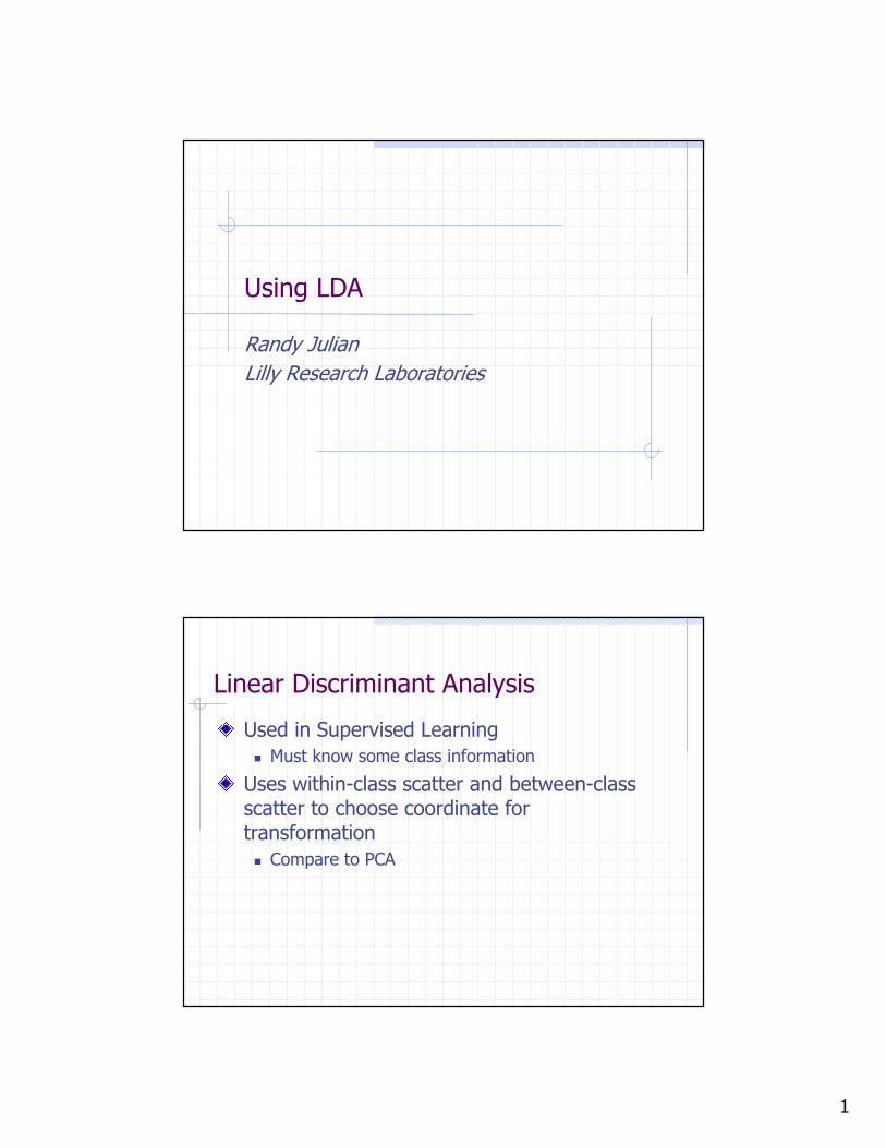
Using LDA

Randy JulianLilly Research Laboratories

Linear Discriminant Analysis

Used in Supervised Learning! Must know some class information

Uses within-class scatter and between-class scatter to choose coordinate for transformation

! Compare to PCA

2

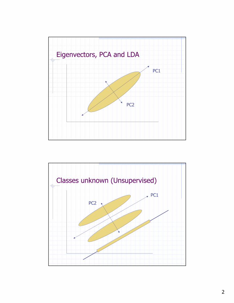
Eigenvectors, PCA and LDA

PC1

PC2

Classes unknown (Unsupervised)

PC1

PC2

3

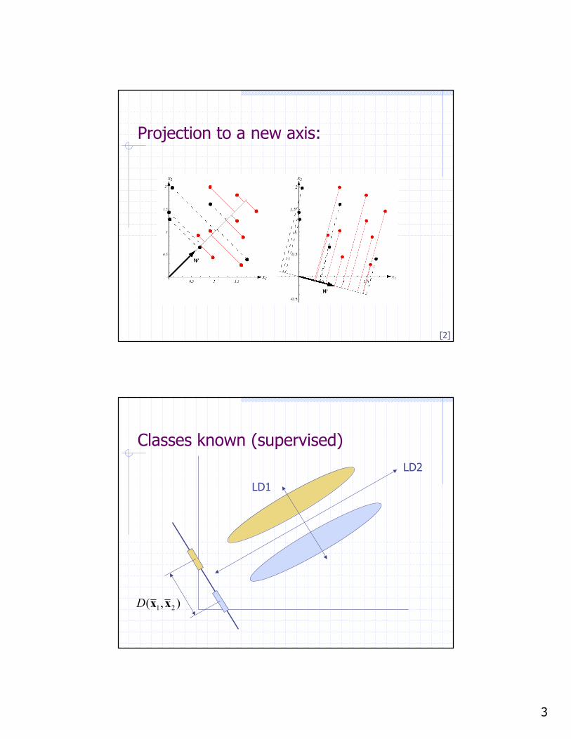
Projection to a new axis:

[2]

Classes known (supervised)LD2

LD1

),( 21 xxD

4

-20 -15 -10 -5 0 5 10 15

-1.5

-1.0

-0.5

0.0

0.5

1.0

1.5

-20-15

-10 -5

0 5

10 15

20

x1

x2

x3

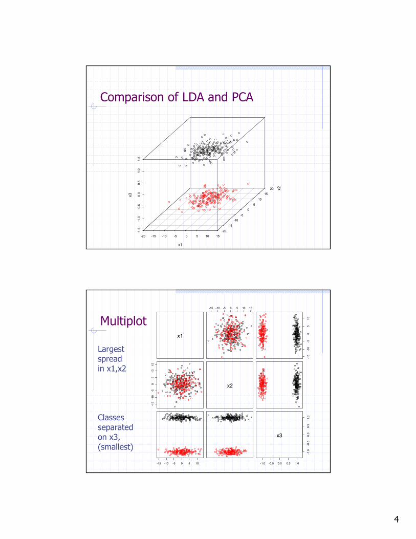
Comparison of LDA and PCA

Multiplotx1

-15 -10 -5 0 5 10 15-1

5-1

0-5

05

10

-15

-10

-50

510

15

x2

-15 -10 -5 0 5 10 -1.0 -0.5 0.0 0.5 1.0

-1.0

-0.5

0.0

0.5

1.0

x3

Largest spreadin x1,x2

Classesseparatedon x3, (smallest)

5

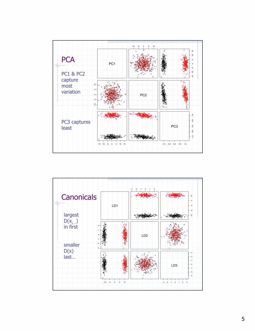
PCAPC1

-10 -5 0 5 10

-15

-10

-50

510

15

-10

-50

510

PC2

-15 -10 -5 0 5 10 15 -1.0 -0.5 0.0 0.5 1.0

-1.0

-0.5

0.0

0.5

1.0

PC3

PC1 & PC2capturemost variation

PC3 capturesleast

CanonicalsLD1

-3 -2 -1 0 1 2-1

0-5

05

10

-3-2

-10

12

LD2

-10 -5 0 5 10 -3 -2 -1 0 1 2 3

-3-2

-10

12

3

LD3

largestD(xi,…)in first

smallerD(x)last…

6

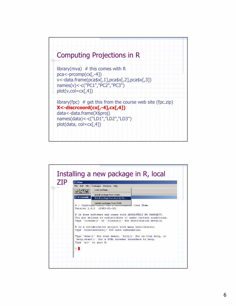
Computing Projections in R

library(mva) # this comes with Rpca<-prcomp(cx[,-4])v<-data.frame(pca$x[,1],pca$x[,2],pca$x[,3])names(v)<-c("PC1","PC2","PC3")plot(v,col=cx[,4])

library(fpc) # get this from the course web site (fpc.zip)X<-discrcoord(cx[,-4],cx[,4])data<-data.frame(X$proj)names(data)<-c("LD1","LD2","LD3")plot(data, col=cx[,4])

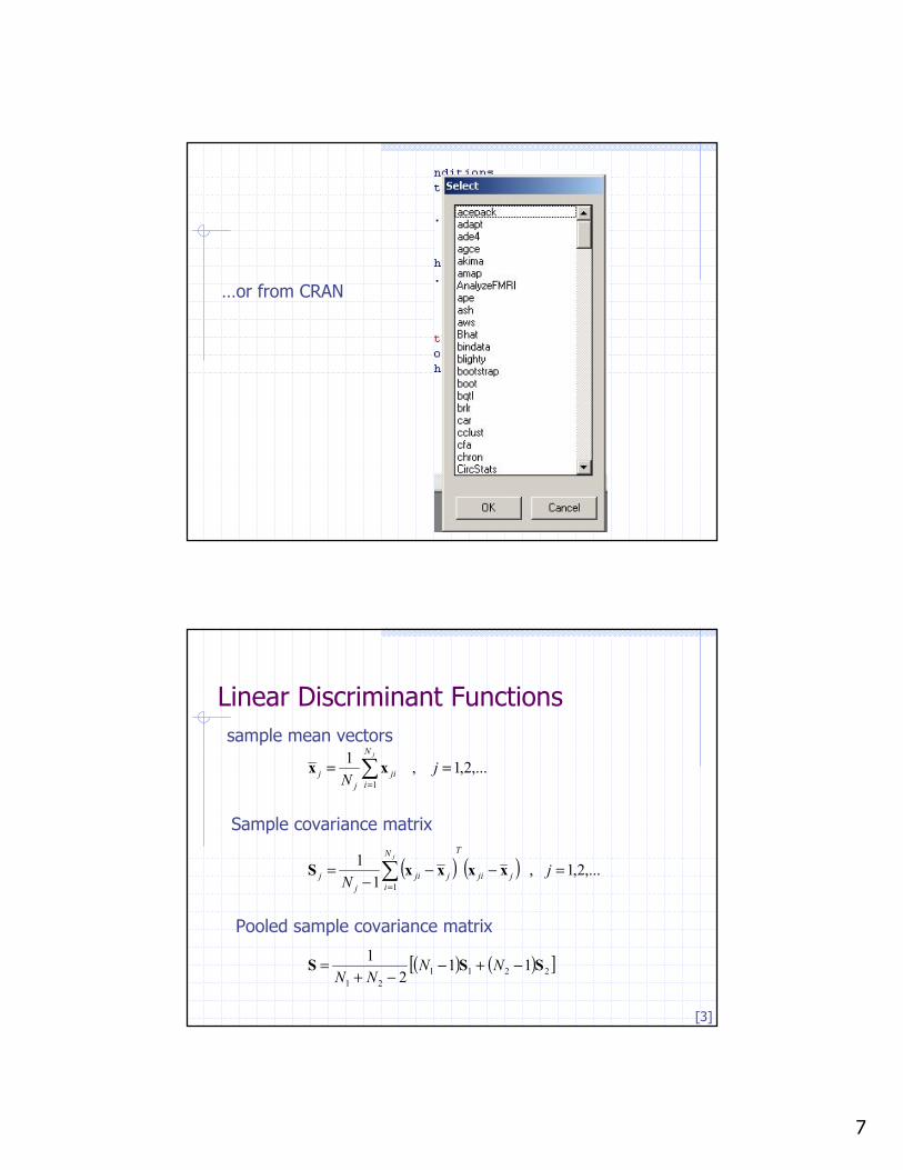
Installing a new package in R, local ZIP

7

…or from CRAN

Linear Discriminant Functions

( ) ( )

( ) ( )[ ]221121

1

1

112

1

,...2,1 , 1

1

,...2,1 , 1

SSS

xxxxS

xx

!+!!+

=

=!!!

=

==

!

!

=

=

NNNN

jN

jN

jji

TN

ijji

jj

N

iji

jj

j

j

sample mean vectors

Sample covariance matrix

Pooled sample covariance matrix

[3]

8

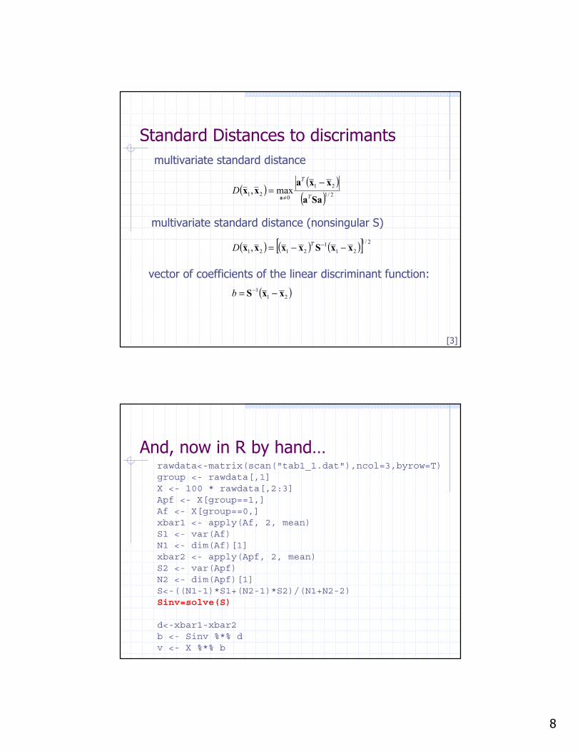
Standard Distances to discrimants

( ) ( )( )

( ) ( ) ( )[ ]

( )211

2/1

211

2121

2/121

021

,

max,

xxS

xxSxxxx

Saa

xxaxx

a

!=

!!=

!=

!

!

"

b

D

D

T

T

T

multivariate standard distance

multivariate standard distance (nonsingular S)

vector of coefficients of the linear discriminant function:

[3]

And, now in R by hand…rawdata<-matrix(scan("tab1_1.dat"),ncol=3,byrow=T)group <- rawdata[,1]X <- 100 * rawdata[,2:3]Apf <- X[group==1,]Af <- X[group==0,]xbar1 <- apply(Af, 2, mean)S1 <- var(Af)N1 <- dim(Af)[1]xbar2 <- apply(Apf, 2, mean)S2 <- var(Apf)N2 <- dim(Apf)[1]S<-((N1-1)*S1+(N2-1)*S2)/(N1+N2-2)Sinv=solve(S)

d<-xbar1-xbar2b <- Sinv %*% dv <- X %*% b

9

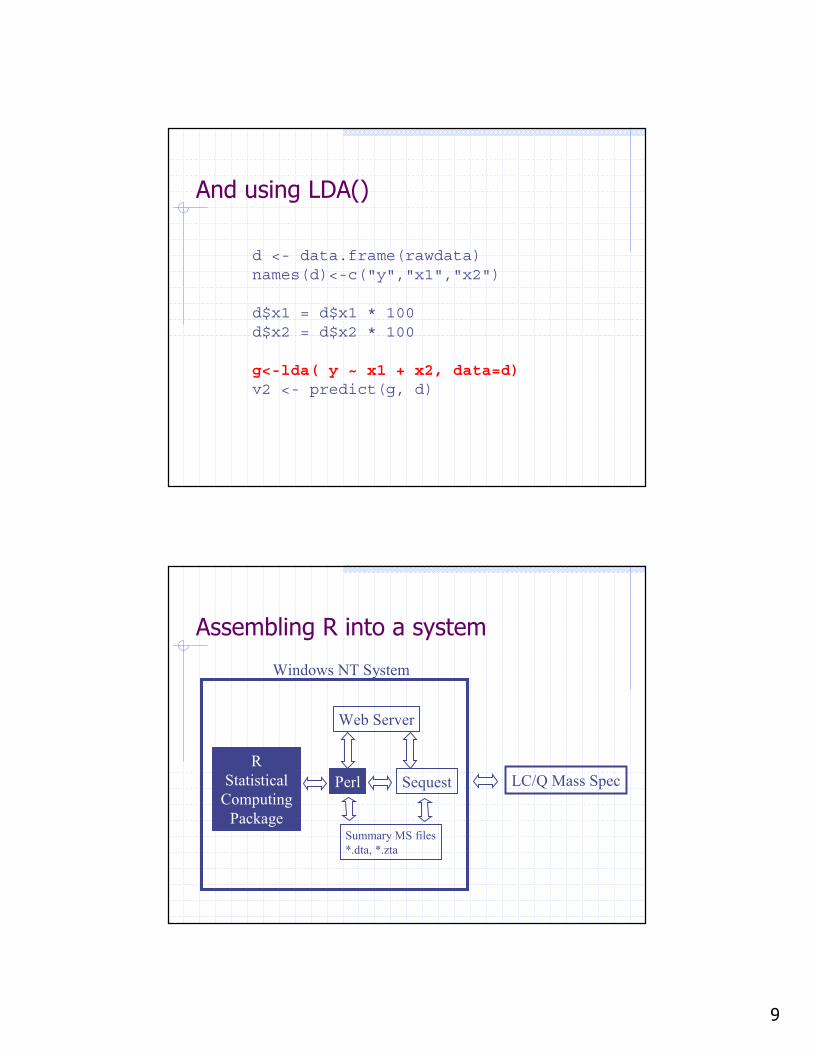
And using LDA()

d <- data.frame(rawdata)names(d)<-c("y","x1","x2")

d$x1 = d$x1 * 100d$x2 = d$x2 * 100

g<-lda( y ~ x1 + x2, data=d)v2 <- predict(g, d)

Assembling R into a system

R Statistical

Computing Package

Perl

Windows NT System

Sequest

Summary MS files*.dta, *.zta

Web Server

LC/Q Mass Spec

10

120 130 140 150

170

180

190

200

X[,1]

X[,2

]

123 4

5 6 7

8

9

1

2

3 45 6

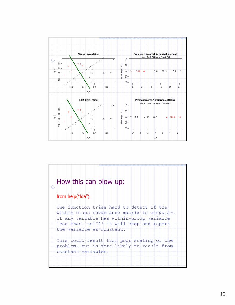
Manual Calculation

120 130 140 150

170

180

190

200

X[,1]

X[,2

]

123 4

5 6 7

8

9

1

2

3 45 6

LDA Calculation

-5 0 5 10 15 20

-1.0

-0.5

0.0

0.5

1.0

v

rep.

0..le

ngth

.v.1

...

123 45 6 78 9123 45 6

Projection onto 1st Canonical (manual)beta_1= 0.58 beta_2= -0.38

-3 -2 -1 0 1 2 3

-1.0

-0.5

0.0

0.5

1.0

LD1

rep.

0..le

ngth

.v.1

...

Projection onto 1st Canonical (LDA)beta_1= -0.15 beta_2= 0.097

1 2 34 567 89 12 34 56

How this can blow up:

from help(“lda”)

The function tries hard to detect if the within-class covariance matrix is singular. If any variable has within-group variance less than `tol^2' it will stop and report the variable as constant.

This could result from poor scaling of the problem, but is more likely to result from constant variables.

11

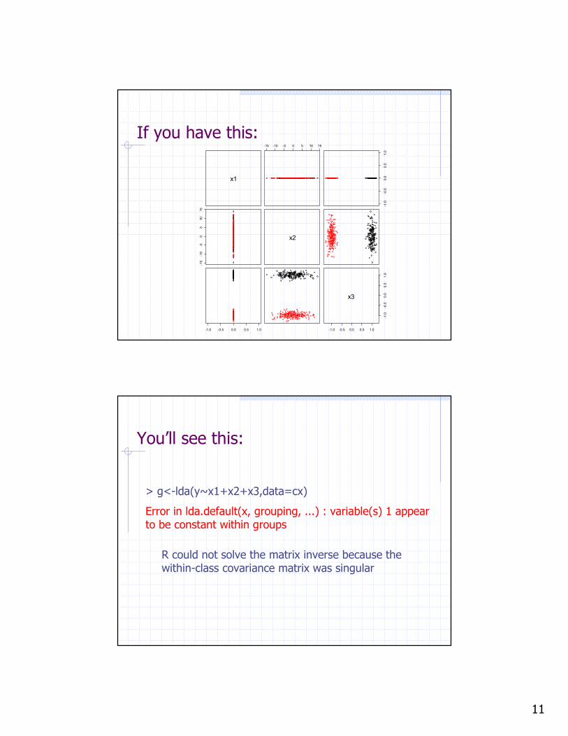
If you have this:

x1

-15 -10 -5 0 5 10 15

-1.0

-0.5

0.0

0.5

1.0

-15

-10

-50

510

15

x2

-1.0 -0.5 0.0 0.5 1.0 -1.0 -0.5 0.0 0.5 1.0

-1.0

-0.5

0.0

0.5

1.0

x3

You’ll see this:

> g<-lda(y~x1+x2+x3,data=cx)

Error in lda.default(x, grouping, ...) : variable(s) 1 appear to be constant within groups

R could not solve the matrix inverse because thewithin-class covariance matrix was singular

12

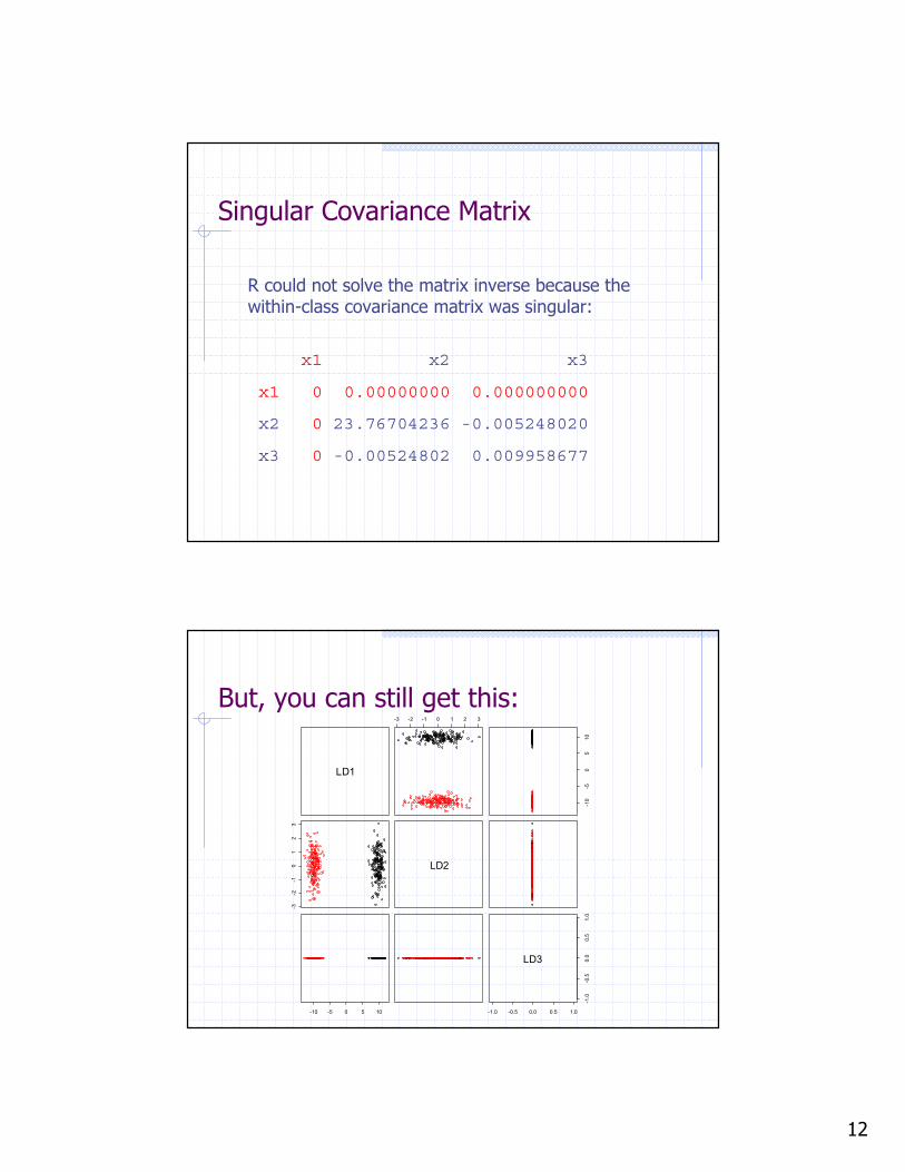
Singular Covariance Matrix

x1 x2 x3

x1 0 0.00000000 0.000000000

x2 0 23.76704236 -0.005248020

x3 0 -0.00524802 0.009958677

R could not solve the matrix inverse because thewithin-class covariance matrix was singular:

But, you can still get this:

LD1

-3 -2 -1 0 1 2 3

-10

-50

510

-3-2

-10

12

3

LD2

-10 -5 0 5 10 -1.0 -0.5 0.0 0.5 1.0

-1.0

-0.5

0.0

0.5

1.0

LD3

13

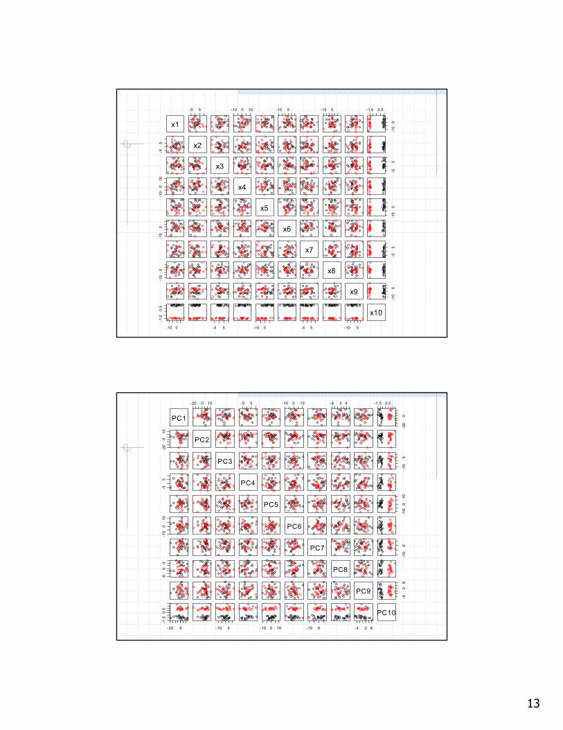
x1

-5 5 -10 0 10 -15 0 -15 0 -1.0 0.5

-10

0

-55 x2

x3

-55

-10

010

x4

x5

-10

0

-15

0 x6

x7

-55

-15

0 x8

x9

-10

5

-10 0

-1.0

0.5

-5 5 -10 0 -5 5 -10 5

x10

PC1

-20 -5 10 -5 5 -10 0 10 -6 0 4 -1.5 0.5-2

00

-20

-510

PC2

PC3

-10

5

-55

PC4

PC5

-10

010

-10

010

PC6

PC7

-10

0

-60

4

PC8

PC9

-42

6

-20 0

-1.5

0.5

-10 5 -10 0 10 -10 0 -4 2 6

PC10

14

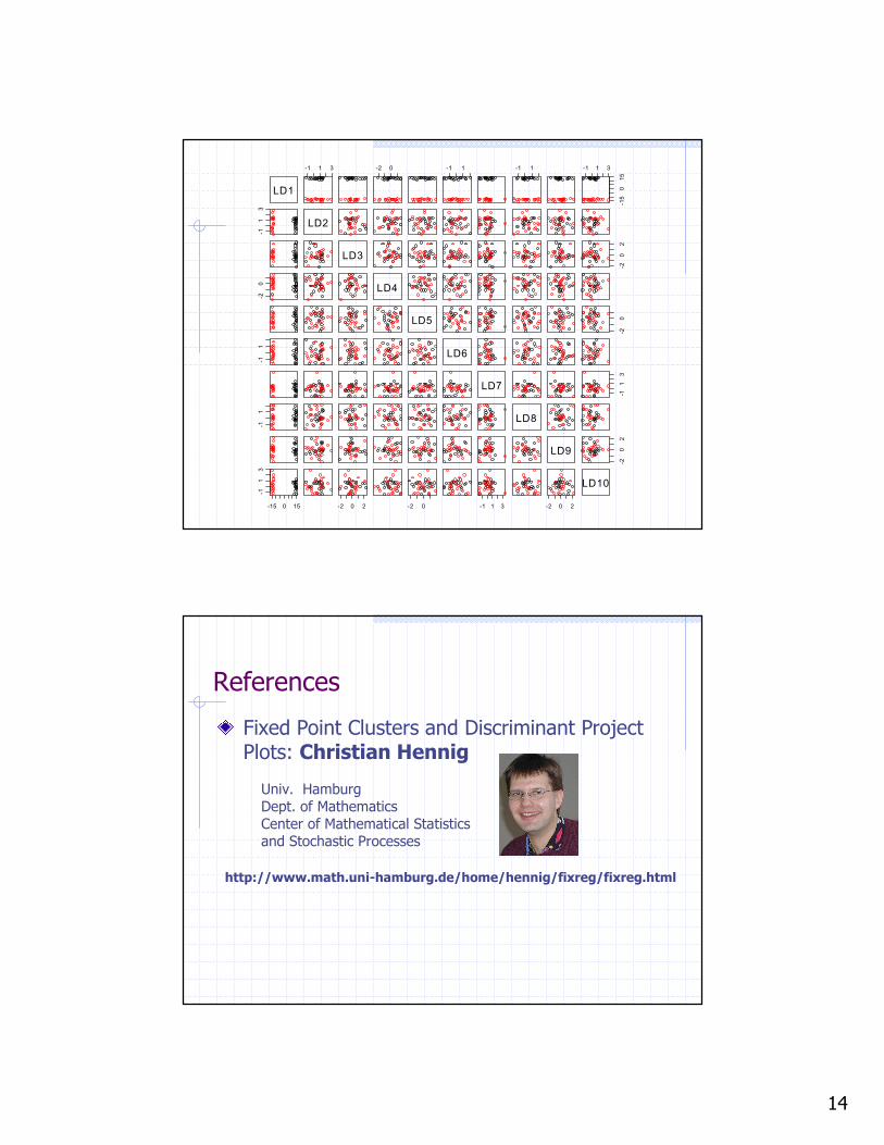
LD1

-1 1 3 -2 0 -1 1 -1 1 -1 1 3

-15

015

-11

3

LD2

LD3

-20

2

-20 LD4

LD5

-20

-11

LD6

LD7

-11

3

-11

LD8

LD9

-20

2

-15 0 15

-11

3

-2 0 2 -2 0 -1 1 3 -2 0 2

LD10

References

Fixed Point Clusters and Discriminant Project Plots: Christian Hennig

http://www.math.uni-hamburg.de/home/hennig/fixreg/fixreg.html

Univ. HamburgDept. of MathematicsCenter of Mathematical Statistics and Stochastic Processes