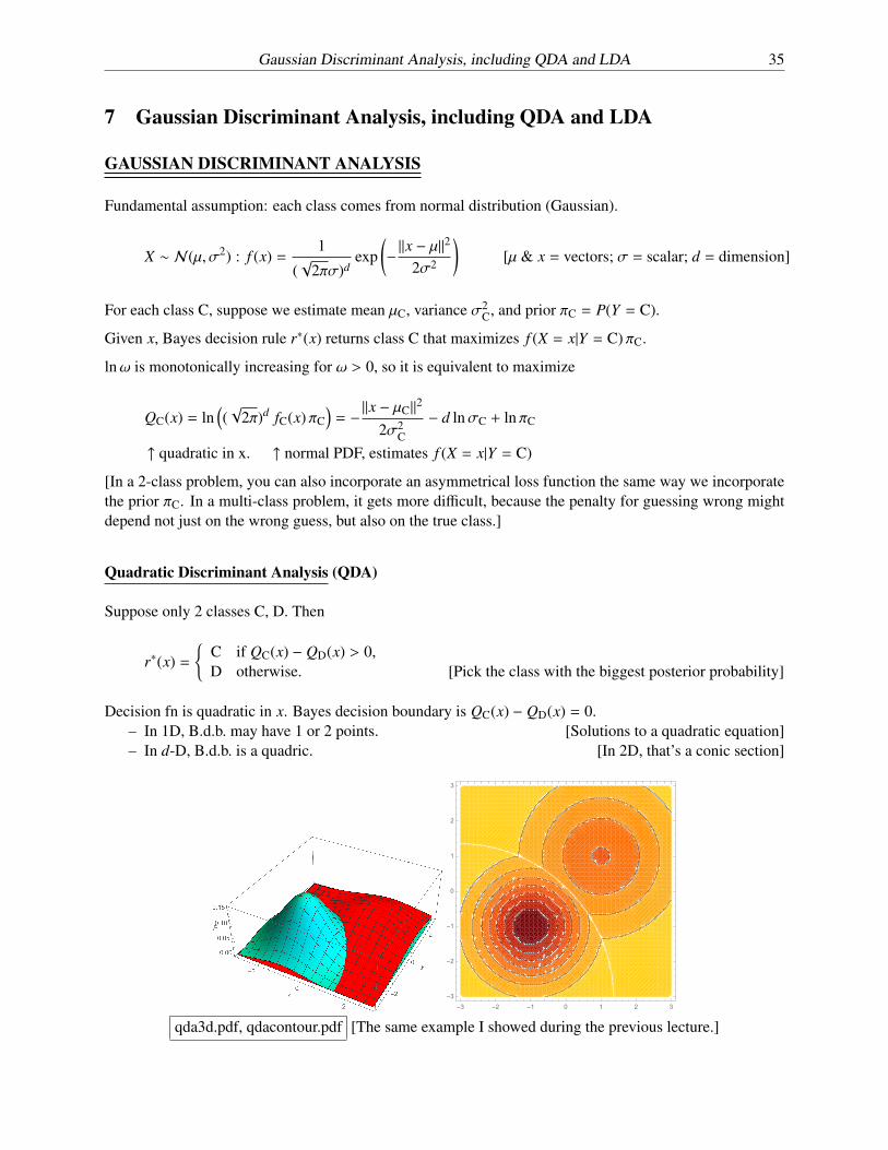
Gaussian Discriminant Analysis, including QDA and LDA 35

7 Gaussian Discriminant Analysis, including QDA and LDA

GAUSSIAN DISCRIMINANT ANALYSIS

Fundamental assumption: each class comes from normal distribution (Gaussian).

X ⇠ N(µ,�2) : f (x) =1

(p

2⇡�)dexp

�kx � µk

2

2�2

![µ & x = vectors; � = scalar; d = dimension]

For each class C, suppose we estimate mean µC, variance �2C, and prior ⇡C = P(Y = C).

Given x, Bayes decision rule r⇤(x) returns class C that maximizes f (X = x|Y = C) ⇡C.

ln! is monotonically increasing for ! > 0, so it is equivalent to maximize

QC(x) = ln⇣(p

2⇡)d fC(x) ⇡C⌘= �kx � µCk2

2�2C� d ln�C + ln ⇡C

" quadratic in x. " normal PDF, estimates f (X = x|Y = C)

[In a 2-class problem, you can also incorporate an asymmetrical loss function the same way we incorporatethe prior ⇡C. In a multi-class problem, it gets more di�cult, because the penalty for guessing wrong mightdepend not just on the wrong guess, but also on the true class.]

Quadratic Discriminant Analysis (QDA)

Suppose only 2 classes C, D. Then

r⇤(x) =(

C if QC(x) � QD(x) > 0,D otherwise. [Pick the class with the biggest posterior probability]

Decision fn is quadratic in x. Bayes decision boundary is QC(x) � QD(x) = 0.– In 1D, B.d.b. may have 1 or 2 points. [Solutions to a quadratic equation]– In d-D, B.d.b. is a quadric. [In 2D, that’s a conic section]

-3 -2 -1 0 1 2 3-3

-2

-1

0

1

2

3

qda3d.pdf, qdacontour.pdf [The same example I showed during the previous lecture.]

36 Jonathan Richard Shewchuk

[You’re probably familiar with the Gaussian distribution where x and µ are scalars, but as I’ve written it, itapplies equally well to a multi-dimensional feature space with isotropic Gaussians. Then x and µ are vectors,but the variance � is still a scalar. Next lecture we’ll look at anisotropic Gaussian distributions where thevariance is di↵erent along di↵erent directions.]

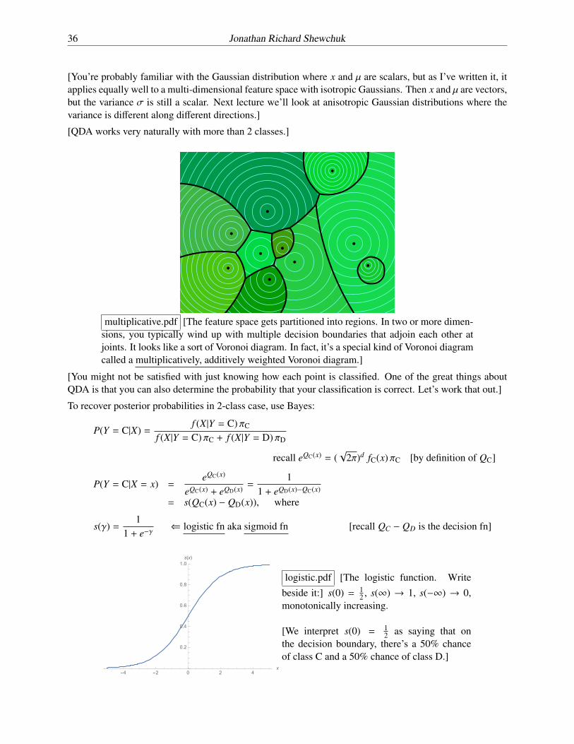
[QDA works very naturally with more than 2 classes.]

multiplicative.pdf [The feature space gets partitioned into regions. In two or more dimen-sions, you typically wind up with multiple decision boundaries that adjoin each other atjoints. It looks like a sort of Voronoi diagram. In fact, it’s a special kind of Voronoi diagramcalled a multiplicatively, additively weighted Voronoi diagram.]

[You might not be satisfied with just knowing how each point is classified. One of the great things aboutQDA is that you can also determine the probability that your classification is correct. Let’s work that out.]

To recover posterior probabilities in 2-class case, use Bayes:

P(Y = C|X) =f (X|Y = C) ⇡C

f (X|Y = C) ⇡C + f (X|Y = D) ⇡D

recall eQC(x) = (p

2⇡)d fC(x) ⇡C [by definition of QC]

P(Y = C|X = x) =eQC(x)

eQC(x) + eQD(x) =1

1 + eQD(x)�QC(x)

= s(QC(x) � QD(x)), where

s(�) =1

1 + e��( logistic fn aka sigmoid fn [recall QC � QD is the decision fn]

-4 -2 0 2 4x

0.2

0.4

0.6

0.8

1.0s(x)

logistic.pdf [The logistic function. Writebeside it:] s(0) = 1

2 , s(1) ! 1, s(�1) ! 0,monotonically increasing.

[We interpret s(0) = 12 as saying that on

the decision boundary, there’s a 50% chanceof class C and a 50% chance of class D.]

Gaussian Discriminant Analysis, including QDA and LDA 37

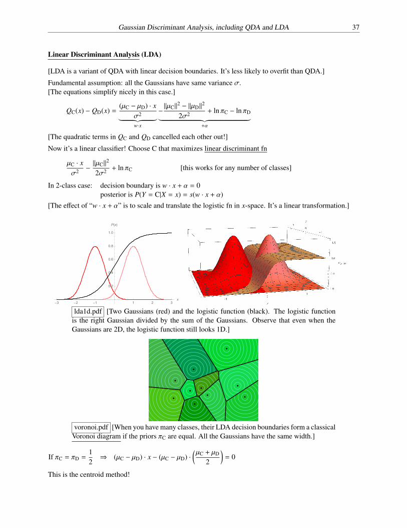
Linear Discriminant Analysis (LDA)

[LDA is a variant of QDA with linear decision boundaries. It’s less likely to overfit than QDA.]

Fundamental assumption: all the Gaussians have same variance �.[The equations simplify nicely in this case.]

QC(x) � QD(x) =(µC � µD) · x

�2| {z }w·x

�kµCk2 � kµDk22�2 + ln ⇡C � ln ⇡D

| {z }+↵

[The quadratic terms in QC and QD cancelled each other out!]

Now it’s a linear classifier! Choose C that maximizes linear discriminant fn

µC · x�2 � kµCk2

2�2 + ln ⇡C [this works for any number of classes]

In 2-class case: decision boundary is w · x + ↵ = 0posterior is P(Y = C|X = x) = s(w · x + ↵)

[The e↵ect of “w · x + ↵” is to scale and translate the logistic fn in x-space. It’s a linear transformation.]

-3 -2 -1 1 2 3x

0.2

0.4

0.6

0.8

1.0

P(x)

lda1d.pdf [Two Gaussians (red) and the logistic function (black). The logistic functionis the right Gaussian divided by the sum of the Gaussians. Observe that even when theGaussians are 2D, the logistic function still looks 1D.]

voronoi.pdf [When you have many classes, their LDA decision boundaries form a classicalVoronoi diagram if the priors ⇡C are equal. All the Gaussians have the same width.]

If ⇡C = ⇡D =12) (µC � µD) · x � (µC � µD) ·

✓µC + µD

2

◆= 0

This is the centroid method!

38 Jonathan Richard Shewchuk

MAXIMUM LIKELIHOOD ESTIMATION OF PARAMETERS (Ronald Fisher, circa 1912)

[To use Gaussian discriminant analysis, we must first fit Gaussians to the sample points and estimate theclass prior probabilities. We’ll do priors first—they’re easier, because they involve a discrete distribution.Then we’ll fit the Gaussians—they’re less intuitive, because they’re continuous distributions.]

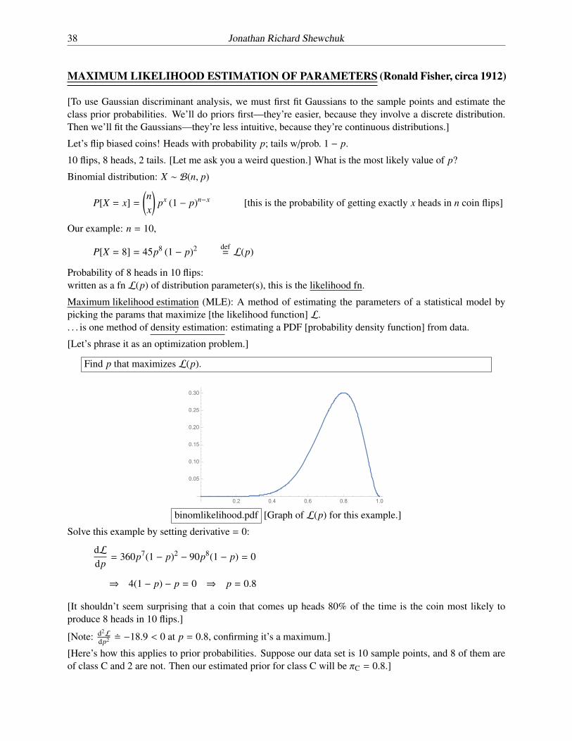
Let’s flip biased coins! Heads with probability p; tails w/prob. 1 � p.

10 flips, 8 heads, 2 tails. [Let me ask you a weird question.] What is the most likely value of p?

Binomial distribution: X ⇠ B(n, p)

P[X = x] = nx

!px (1 � p)n�x [this is the probability of getting exactly x heads in n coin flips]

Our example: n = 10,

P[X = 8] = 45p8 (1 � p)2 def= L(p)

Probability of 8 heads in 10 flips:written as a fn L(p) of distribution parameter(s), this is the likelihood fn.

Maximum likelihood estimation (MLE): A method of estimating the parameters of a statistical model bypicking the params that maximize [the likelihood function] L.. . . is one method of density estimation: estimating a PDF [probability density function] from data.

[Let’s phrase it as an optimization problem.]

Find p that maximizes L(p).

0.2 0.4 0.6 0.8 1.0

0.05

0.10

0.15

0.20

0.25

0.30

binomlikelihood.pdf [Graph of L(p) for this example.]

Solve this example by setting derivative = 0:

dLdp= 360p7(1 � p)2 � 90p8(1 � p) = 0

) 4(1 � p) � p = 0 ) p = 0.8

[It shouldn’t seem surprising that a coin that comes up heads 80% of the time is the coin most likely toproduce 8 heads in 10 flips.]

[Note: d2Ldp2 ⌘ �18.9 < 0 at p = 0.8, confirming it’s a maximum.]

[Here’s how this applies to prior probabilities. Suppose our data set is 10 sample points, and 8 of them areof class C and 2 are not. Then our estimated prior for class C will be ⇡C = 0.8.]

Gaussian Discriminant Analysis, including QDA and LDA 39

Likelihood of a Gaussian

Given sample points X1, X2, . . . , Xn, find best-fit Gaussian.

[Now we want a normal distribution instead of a binomial distribution. If you generate a random point froma normal distribution, what is the probability that it will be exactly at the mean of the Gaussian?]

[Zero. So it might seem like we have a problem here. With a continuous distribution, the probability ofgenerating any particular point is zero. But we’re just going to ignore that and do “likelihood” anyway.]

Likelihood of generating these points is

L(µ,�; X1, . . . , Xn) = f (X1) f (X2) · · · f (Xn). [How do we maximize this?]

The log likelihood `(·) is the ln of the likelihood L(·).Maximizing likelihood , maximizing log likelihood.

`(µ,�; X1, ..., Xn) = ln f (X1) + ln f (X2) + ... + ln f (Xn)

=

nX

i=1

�kXi � µk2

2�2 � d lnp

2⇡ � d ln�!

| {z }ln of normal PDF

Want to set rµ` = 0,@`

@�= 0

rµ` =nX

i=1

Xi � µ�2 = 0 ) µ̂ =

1n

nX

i=1

Xi [The hats ˆ mean “estimated”]

@`

@�=

nX

i=1

kXi � µk2 � d�2

�3 = 0 ) �̂2 =1

dn

nX

i=1

kXi � µk2

We don’t know µ exactly, so substitute µ̂ for µ to compute �̂.

I.e., we use mean & variance of points in class C to estimate mean & variance of Gaussian for class C.

For QDA: estimate conditional mean µ̂C & conditional variance �̂2C of each class C separately [as above]

& estimate the priors:

⇡̂C =nCPD nD ( total sample points in all classes [⇡̂C is the coin flip parameter]

For LDA: same means & priors; one variance for all classes:

�̂2 =1

dn

X

C

X

{i:yi=C}kXi � µ̂Ck2 ( pooled within-class variance

[Notice that although LDA is computing one variance for all the data, each sample point contributes withrespect to its own class’s mean. This gives a very di↵erent result than if you simply use the global mean!It’s usually smaller than the global variance. We say “within-class” because we use each point’s distancefrom its class’s mean, but “pooled” because we then pool all the classes together.]