101 Basics Hands-On Experimental work notes

Species Distribution Modeling

101

Basics Hands-On

Experimental work notes

Rita Castilho

May 2015

SDM101 Rita Castilho

Page | 1

SDM101. IMPLEMENTATION OF BASIC STEPS

Species distribution modelling (SDM) is a recent scientific development that has enormous application potential in biological sciences. Most of the information on the geographic distribution of species stems from fieldwork data accumulated throughout centuries. Species distribution modelling is also known under other names including climate envelope-modelling, habitat modelling, and environmental or ecological niche-modelling (ENM). The advent of SDM has allowed inferring hypothetical geographic species’ distributions by relating the presence or presence and absence of a species with environmental variables (Franklin 2010). It is possible to predict the environmental conditions that are suitable for a species by classifying grid cells according to the degree in which they are suitable/unsuitable for a species, resulting in a predictive model describing the suitability of any site for that species (Guisan & Thuiller 2005). Common applications of SDM include exploring the response of geographic species distributions to climate change (Peterson 2011), predicting range expansions of invasive species (Benedict et al. 2009), supporting conservation planning (Wilson et al. 2011), identifying areas of endemism (Raxworthy et al. 2007) and facilitating field surveys of species with poorly known geographic distributions (Guisan & Thuiller 2005; Raxworthy et al. 2003). Different implementations of SDM This experimental work provides an introduction to the making of species distribution modelling with R. It is largely based on two different approaches: i) WALLACE beta v0.1: Harnessing Digital Biodiversity Data for Predictive Modelling, fuelled by R (http://protea.eeb.uconn.edu:3838/wallace/) and ii) Hijmans and Elith (Hijmans et al. 2014) “Species distribution modelling with R” (http://cran.r-project.org/web/packages/dismo/vignettes/sdm.pdf). Our goal is to provide practical guidance to implement the basic steps of SDM not to provide the theoretical background on SDM. You will not have any problems in finding background references on the subject. Workflow of SDM There are lots of different ways to go about SDM, however, the general workflow for obtaining an SDM is: (0) Choose a target species. You may do so because you are already working on a given species, or will be working on that species in the future. However, if this is not the case, you still need to choose a species... (1) Collect the locations (geographical coordinates) of occurrence of the target species. (2) Assemble values of environmental predictor variables at these locations taken from spatial databases; (3) Use the environmental values to fit a model to estimate similarity to the sites of occurrence; (4) Predict the variable(s) of interest across the region of interest. Steps 0-2 are easy and quick to perform in contrast with steps 3 and 4, which may be complex and long to implement.


Page | 2

WALLACE (beta v0.1) Harnessing Digital Biodiversity Data for Predictive Modeling, fueled by R (http://protea.eeb.uconn.edu:3838/wallace/) The Global Biodiversity Information Facility (GBIF) harnesses numerous species occurrence records, with free access and unlimited downloads for use in your research. You can explore those records by occurrences, species, datasets and countries. Wallace uses these data to generate high-quality models that estimate a species’ abiotic niche requirements and suitable geographic areas. Two main obstacles in estimating the environmental habitat of species are the effects of sampling bias and evaluation of performance of different models. Two R packages, spThin (Aiello‐Lammens et al. 2015) and ENMeval (Muscarella et al. 2014) automate solutions to these obstacles. spThin thin returns spatially thinned species occurence data sets buy a randomizing algorithm to create a data set in which all occurrence locations are at least a fixed distance apart. Spatial thinning helps to reduce the effect of uneven, or biased, species occurence collections on spatial model outcomes. The ENMeval package performs 3 rather relevant tasks in the estimation of SDM: (1) automatically partitions data into training and testing bins, (2) executes ENMs using Maxent (Phillips et al. 2006) with a variety of user-defined settings and (3) estimates multiple metrics to aid in selecting model settings that balance model goodness-of-fit and complexity. However, a gui-mediated (Graphical User Interface (GUI) that calls on the use of GBIF together with R-packages rgbif (Chamberlain et al. 2013), spThin (Aiello‐Lammens et al. 2015), dismo (Hijmans et al. 2014) and ENMeval (Muscarella et al. 2014) first approach to SDM such as “Wallace: Harnessing Digital Biodiversity Data for Predictive Modeling, Fueled by R” is quite useful for the novice. You will be able to download and map GBIF occurrence data, eliminate questionable records, remove clustered records, access climatic variables, build and evaluate Maxent models of varying complexities, visualize predictions, and save results. Wallace can run online or locally (PC/Mac). We advise you have preview the video before setting out to do your first SDM! Wallace has five processes: 1) Download, plot and clean occurrence data The first step is to download occurrence data (e.g. from GBIF; duplicate records are removed). After acquiring these points, it is useful to examine them on a map. Such datasets can contain errors; as a preliminary method of data-cleaning, here the user can specify records to be remove. Additionally, the user can download the records as a CSV file. 2) Process occurrence data Datasets of occurrence records typically suffer from the effects of biased sampling across geography. spThin implements one way to reduce the effects of such biases, by spatial thinning that removes occurrence records less than a user-specified distance from other records. The user can download the thinned records as a CSV file. This step is optional. 3) Choose environmental variables Choice of which environmental variables to use as predictors. These data are in raster form. For this demonstration, WorldClim bioclimatic variables are made available at 3 resolutions. For Maxent and many other niche/distribution modeling approaches, selection of a study region is critical because it defines the pixels whose environmental values are compared with those of the pixels holding occurrence records of the species (Anderson & Raza 2010; Barve et al. 2011). As one way to do so, the user can choose a bounding box or minimum convex polygon around the occurrence records, as well as buffer distance for either.


Page | 3

4) Build and evaluate distribution models The output of niche/distribution models varies greatly depending on model settings, in particular those affecting the level of model complexity. This step automates the tedious building of a suite of candidate models with differing limitations on complexity. Furthermore, it quantifies their performance on test records. These metrics can aid the user in selecting optimal settings. You have several option to choose from:

A. Algorithm Maxent Boosted Regression Trees (not functional) Random Forest (not functional) GAM (not functional)

B. Select feature classes (flexibility of modeled response) To assess model complexity, we additionally fit MaxEnt models using the default settings, which automate the implementation of more complex model feature classes (quadratic, product, hinge, and threshold) depending on the number of occurrence records. See Appendix 2 for a more detailed explanation. L (= linear) LQ (=linear, quadratic) H (=hinge) LQH (=linear, quadratic, hinge) LQHP (=linear, quadratic, hinge, product) LQHPT (=linear, quadratic, hinge, product, threshold)

C. Select regularization multipliers (penalty against complexity) from 1 to 10 Regularization provides a method to reduce model over-fitting. Regularization can be thought of as a smoothing parameter, making the model more regular, so as to avoid fitting too complex a model. In MaxEnt the regularization parameters can be changed if required, where larger values increase the amount of smoothing. For the purpose of this exercise, we will leave the default setting at 1 for this value.

D. Regularization multipliers step value E. Occurrence record partitioning method

(I have tried to come up with an illustrative example, but I could not find one) Jacknife Block Checkerboard 1 Checkerboard 2 Random kfold (not implemented) User-specified (not implemented)

As a start one usually runs the process with the default options (taken from the video). However, we want to know the meaning of each of these options, and therefore 5) View Predictions View the prediction rasters. You can download them individually and import into a GIS for further analysis. Task 1. Run “Wallace” for your target species. You will see at the top of the map the number of duplicated records automatically removed. You have also the chance to remove akward or uncertainpoints, one by one. However, more often than not, there are too many points to eliminate, and a process of automatic removal would be more efficient and practical. Any suggestions? Task 2. Determine the best model. Problems? Task 3. Discuss the limitations of Wallace implementation.


Page | 4

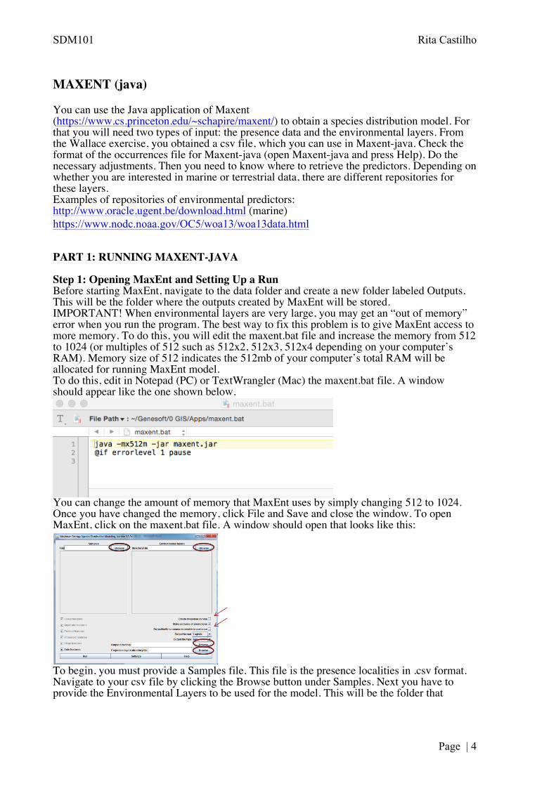
MAXENT (java) You can use the Java application of Maxent (https://www.cs.princeton.edu/~schapire/maxent/) to obtain a species distribution model. For that you will need two types of input: the presence data and the environmental layers. From the Wallace exercise, you obtained a csv file, which you can use in Maxent-java. Check the format of the occurrences file for Maxent-java (open Maxent-java and press Help). Do the necessary adjustments. Then you need to know where to retrieve the predictors. Depending on whether you are interested in marine or terrestrial data, there are different repositories for these layers. Examples of repositories of environmental predictors: http://www.oracle.ugent.be/download.html (marine) https://www.nodc.noaa.gov/OC5/woa13/woa13data.html PART 1: RUNNING MAXENT-JAVA Step 1: Opening MaxEnt and Setting Up a Run Before starting MaxEnt, navigate to the data folder and create a new folder labeled Outputs. This will be the folder where the outputs created by MaxEnt will be stored. IMPORTANT! When environmental layers are very large, you may get an “out of memory” error when you run the program. The best way to fix this problem is to give MaxEnt access to more memory. To do this, you will edit the maxent.bat file and increase the memory from 512 to 1024 (or multiples of 512 such as 512x2, 512x3, 512x4 depending on your computer’s RAM). Memory size of 512 indicates the 512mb of your computer’s total RAM will be allocated for running MaxEnt model. To do this, edit in Notepad (PC) or TextWrangler (Mac) the maxent.bat file. A window should appear like the one shown below.

You can change the amount of memory that MaxEnt uses by simply changing 512 to 1024. Once you have changed the memory, click File and Save and close the window. To open MaxEnt, click on the maxent.bat file. A window should open that looks like this:

To begin, you must provide a Samples file. This file is the presence localities in .csv format. Navigate to your csv file by clicking the Browse button under Samples. Next you have to provide the Environmental Layers to be used for the model. This will be the folder that


Page | 5

contains all your environmental layers in ASCII format (they must have an .asc file extension) with the same geographic bounds, cell size, and projection system. Navigate to this folder by clicking the Browse button under Environmental Layers. Notice how you can change the environmental layers to either continuous or categorical. If any of the layers you include in your environmental layers are categorical (e.g. vegetation type), make sure you change them by clicking on the down arrow and choosing categorical. An Output folder also needs to be selected. This will be the folder where all the MaxEnt outputs will be stored. We will use the folder created earlier named Outputs. Navigate to this folder by clicking the Browse located next to the Output Directory. You can leave the Projection Layers Folder/File window blank if you do not intend on producing future scenarios. Make sure that the Create Response Curves, Make Pictures of Predictions, and Do jackknife to Measure Variable Importance boxes are all checked. Keep the Auto Features box checked and leave the Output Format as Logistic and the Output file type as .asc. Now, the MaxEnt GUI (graphic user interface) should look like this:

Step 2: MaxEnt Settings Choose the Settings sub-tab. Replicates (Number of Runs) MaxEnt allows the ability to run a model multiple times and then conveniently averaging the results from all models created. Using this feature in combination with withholding a certain portion of the data for testing (see Random Test Percentage below) enables the ability to test the model performance while taking advantage of all available data without having an independent dataset. Executing multiple runs also provides a way to measure the amount of variability in the model. To set the replicates in MaxEnt, go to Settings and then enter the number of run in the Replicates field. We will use 3.


Page | 6

Step 3: Random Test Percentage (Test data) (Basic tab) One way to evaluate model performance is to use the Random test percentage setting in MaxEnt. This setting allows you to withhold a certain percentage of your presence data to be used to evaluate the model’s performance. This is important because without these test data, the model will employ data used to develop the model (also called training data) to evaluate the model. This is a bias method and will provide an inflated measure of model performance. There are three different sampling techniques (replicate run types) that are available in MaxEnt: Crossvalidation, Subsampling and bootstrap. We use sub-sample for the majority of the models we run. To select the Subsample replicate run type go to Settings and chose Subsample in the drop down for the field Replicated run type.

NOTE: You will need to check the “Random seed” box when using test data. If you forget to check this, MaxEnt will pop up an error and force you to check this box. Step 4: Reducing disk space and increasing speed (optional setting) (Advanced tab) When the only output needed from a MaxEnt run is the averaged results from multiple runs (replications), you can change the model setting to turn off the “write output grids.” This will prevent MaxEnt from writing output grids from individual runs and only output the summary statistic grids (e.g. Average, Minimum, Maximum, etc.) from all the runs. This will speed up the total run time and decrease disk space. You can turn off the “write output grids” option by going to Settings, selecting the Advanced tab and then de-check write output grids.


Page | 7

Step 5: Number of Iterations (Convergence) (Advanced tab) Normally set to 500, increase this amount to 5000. This allows the model to have adequate time for convergence. If the model doesn’t have enough time to converge, (in the form of number of iterations) the model may over-predict or under-predict the relationships. To increase the amount of iterations go to the MaxEnt Settings select the Advanced tab and then enter 5000 in the field Maximum iterations.


Page | 8

Step 6: Running the MaxEnt model Now that everything has been entered into the MaxEnt program, simply press the Run button to begin modeling. A progress window will appear describing the modeling process. You will also be able to see the gain for each environmental variable while the model is running. The gain is similar to a measure of goodness of fit. Specifically, the gain is a measure of the closeness of the model concentration around the presence samples. So a gain value of 2, would translate to the average likelihood of the presence samples is exp(2) or about 7.5 times higher than that of a random background pixel. Once the MaxEnt model has completed its run, the progress window will disappear. You will be able to find all the outputs created by MaxEnt in the Outputs folder you created earlier. You have now completed a MaxEnt model and can start interpreting the outputs. PART 2: INTERPRETING MAXENT OUTPUTS This part of the tutorial explores the different outputs of MaxEnt. Many, but not all, of MaxEnt’s outputs will be discussed and explained. The layers used for this tutorial were taken from Bio-Oracle (the full list of codes and their bioclimatic variables is attached at the end of this tutorial). For further explanation and interpretation of MaxEnt’s outputs, users should refer to www.cs.princeton.edu/~schapire/maxent/ . Step 1: Exploring MaxEnt Outputs First, open the folder that contains the MaxEnt outputs (i.e. Outputs). When you open the folder, you should see another folder labeled plots, and a list of other files. Open the file called XXX.html file, which has the default browser you use. This is the main output file for the MaxEnt model. This file contains information on the overall averaging of all model runs that were specified with statistical analyses, plots, model images, and links to the other files and runs. Also contained in this file are the control settings and parameters that were used to run the model, and the code to run the MaxEnt model from the command line. The first graph you see in this file is the Analysis of Omission/ Commission. The “25” we entered for “random test percentage” told the program to randomly set aside 25% of the sample records for testing. This allows the program to do some simple statistical analysis. Much of the analysis used the use of a threshold to make a binary prediction, with suitable conditions predicted above the threshold and unsuitable below. The first plot shows how testing and omission (training) and predicted area vary with the choice of cumulative threshold. The orange and blue shading surrounding the lines on the graph represent variability. Here we see that the omission on test samples (orange) is a very good match to the predicted (black) omission rate. In some situations, the test omission line lies well below the predicted omission line: a common reason is that the test and training data are not independent, for example if they derive from the same spatially autocorrelated presence data. On the left the result of a 15 replicate run, on the right the result of a 5 replicate run.

The next graph you see when you scroll down is the Sensitivity vs 1 –Specificity. This is a graph of the Area Under the Receiver Operating Characteristic (ROC) Curve or AUC. The AUC values allow you to easily compare performance of one model with another, and are useful in evaluating multiple MaxEnt models. An AUC value of 0.5 indicates that the performance of the model is no better than random, while values closer to 1.0 indicate better model performance.


Page | 9

Further down the page, you will see a picture of the model. You can click on the picture to see an enlarged version. You can also find this image in the Plots folder in the outputs as a Portable Network Graphic (.png) file.

Which variables matter most? A natural application of species distribution modeling is to answer the question, which variables matter most for the species being modeled? There is more than one way to answer this question; here we outline the possible ways in which Maxent can be used to address it. While the Maxent model is being trained, it keeps track of which environmental variables are contributing to fitting the model. Each step of the Maxent algorithm increases the gain of the model by modifying the coefficient for a single feature; the program assigns the increase in the gain to the environmental variable(s) that the feature depends on. Converting to percentages at the end of the training process, we get the middle column in the table below. Farther down the page, you will see a table that shows the Analysis of Variable Contributions. This table shows the environmental variables used in the model and their percent predictive contribution of each variable. The higher the contribution, the more impact that particular variable has on predicting the occurrence of that species. In this example sea surface temperature range (i.e. sstrange) had the highest predictive contribution of 37.6%. Below the variable contributions is a graph of the Jackknife of Regularized Training Gain. The jackknifing shows the training gain of each variable if the model was run in isolation, and


Page | 10

compares it to the training gain with all the variables. This is useful to identify which variables contribute the most individually. In this case, the environmental variable with highest gain when used in isolation is sstrange, which therefore appears to have the most useful information by itself. The environmental variable that decreases the gain the most when it is omitted is phosphate, which therefore appears to have the most information that isn't present in the other variables. Turning to the lighter blue bars, it appears that no variable contains a substantial amount of useful information that is not already contained in the other variables, because omitting each variable in turn did not decrease the training gain considerably.Values shown are averages over replicate runs. The model also provides a jackknife for test gain of the species and AUC.

If you use the same data for training and for testing then the red and blue lines will be identical. If you split your data into two partitions, one for training and one for testing it is normal for the red (training) line to show a higher AUC than the blue (testing) line. The red (training) line shows the “fit” of the model to the training data. The blue (testing) line indicates the fit of the model to the testing data, and is the real test of the models predictive power.

It is important to note that AUC values tend to be higher for species with narrow ranges, relative to the study area described by the environmental data. This does not necessarily mean that the models are better; instead this behavior is an artifact of the AUC statistic.

Task 1. Appraisal of the most and the least relevant variables

Observe the graphs below for a given species, and identify the most important and less important variable for predicting the distribution of the occurrence data.


Page | 11

We see that if Maxent uses only pre6190_l1 (average January rainfall) it achieves almost no gain, so that variable is not (by itself) useful for estimating the distribution of Bradypus. October rainfall (pre6190_l10) allows a reasonably good fit to the training data. Turning to the lighter blue bars, it appears that no variable contains a substantial amount of useful information that is not already contained in the other variables, because omitting each variable in turn did not decrease the training gain considerably. However, if we would have to remove variables from the analysis, h_dem would be the chosen variable. Comparing the three jackknife plots can be very informative. The AUC plot shows that annual precipitation (pre6190_ann) is the most effective single variable for predicting the distribution of the occurrence data that was set aside for testing, when predictive performance is measured using AUC, even though it was hardly used by the model built using all variables. The relative importance of annual precipitation also increases in the test gain plot, when compared against the training gain plot. In addition, in the test gain and AUC plots, some of the light blue bars (especially for the monthly precipitation variables) are longer than the red bar, showing that predictive performance improves when the corresponding variables are not used. This tells us that these (monthly precipitation) variables are helping Maxent to obtain a good fit to the training data, but the annual precipitation variable generalizes better, giving comparatively better results on the set-aside test data. Phrased differently, models made with the monthly precipitation variables appear to be less transferable. This is important if our goal is to transfer the model, for example by applying the model to future climate variables in order to estimate its future distribution under climate change. It makes sense that monthly precipitation values are less transferable: likely suitable conditions for this species will depend not on precise rainfall values in selected months, but on the aggregate average rainfall, and perhaps on rainfall consistency or lack of extended dry periods. When we are modeling on a continental scale, there will probably be shifts in the precise timing of seasonal rainfall patterns, affecting the monthly precipitation but not suitable conditions for the species. The same line of thought can be pursued when dealing with a marine species. Sea surface temperature for particular months may not be as good descriptor variables as sea surface temperature range, or minimum or maximum values. Bio-Oracle has these aggregate variables while World Ocean Atlas (https://www.nodc.noaa.gov/OC5/woa13/woa13data.html) has another king of aggregation (see below).


Page | 12

In general, it would be better to use variables that are more likely to be directly relevant to the species being modeled. For example, the Worldclim website (www.worldclim.org) provides “BIOCLIM” variables, including derived variables such as “rainfall in the wettest quarter”, rather than monthly values. A last note on the jackknife outputs: the test gain plot shows that a model made only with January precipitation (pre6190_l1) results in a negative test gain. This means that the model is slightly worse than a null model (i.e., a uniform distribution) for predicting the distribution of occurrences set aside for testing. This can be regarded as more evidence that the monthly precipitation values are not the best choice for predictor variables. Task 2. Run Maxent-java for your target species. Identify specific problems or advantages.


Page | 13

SDM BY SCRIPTING

1. SPECIES OCCURRENCE RECORDS

HOW TO COLLECT THE LOCATIONS (GEOGRAPHICAL COORDINATES ) OF OCCURRENCE OF THE TARGET SPECIES?

There are several ways to get presence data from the target species: (1) databases: Gbif (http://www.gbif.org), Obis (http://iobis.org/), Fishbase (http://fishbase.org); (2) previous published work ; and (3) own work. There are several problems with using data retrieved from databases, mostly related to either duplicate data and georeferencing errors, for instance data relating to marine species that is georeferenced in land or the other way around. Errors are identified by creating an overlay between the point locality layer and a maritime boundaries layer (coastlines) provided by the data(wrld_simpl). Any mismatch between these layers was indicative of a potential georeferencing error and outlying points can be removed. We will use a script that automatically retrieves data from these two databases (marine organisms), eliminates the duplicates and eliminates all the inland or marine points, depending on the species, written by Miguel Gandra. ################################################################################################################### ## Miguel Gandra || [email protected] || April 2015 ############################################################## ################################################################################################################### # Script to plot a distribution map of a chosen species from GBIF, OBIS and FishBase records. # http://www.gbif.org # http://iobis.org # http://www.fishbase.org # ---> no prior file manipulation required # ---> automatically distinguishes points on land and sea, plotting them with different colors # ---> automatically saves a pdf file with the map on the chosen directory # ---> exports a csv file with the fetched coordinates # ---> prints a summary of the records # 1. Define the genus and species name in the variables field (below). # 2. Set the directory containing the data files (txt from GBIF and csv from OBIS) - user's desktop predefined. # GBIF data: the script first looks for the "occurrence.txt" file in the chosen directory, # if it's not available or contains wrong species, the data is downloaded directly from the GBIF portal. # OBIS data: the script looks for a csv file in the chosen directory (if multiple csv files are found # it uses the first one listed). # FishBase data: the script downloads the data directly from the web. # The "marginal.tolerance" variable sets the margin at which records are considered to be in land. # A positive value will consider records to be on land, even if they are up to x degrees outside the nearest coast. # A negative value will constraint land records to the ones that are at least x degrees within the coastline. # User can automatically delete points in land by setting the "remove.land.points" variable to TRUE, # or delete points in water by setting the "remove.ocean.points" variable to TRUE. ###################################################################################### # Automatically install required libraries ########################################## # (check http://tlocoh.r-forge.r-project.org/mac_rgeos_rgdal.html # if rgeos and rgdal installation fails on a Mac) if(!require(dismo)){install.packages("dismo"); library(dismo)}


Page | 14

if(!require(XML)){install.packages("XML"); library(XML)} if(!require(jsonlite)){install.packages("jsonlite"); library(jsonlite)} if(!require(graphics)){install.packages("graphics"); library(graphics)} if(!require(maps)){install.packages("maps"); library(maps)} if(!require(maptools)){install.packages("maptools"); library(maptools)} if(!require(rgeos)){install.packages("rgeos"); library(rgeos)} if(!require(rgdal)){install.packages("rgdal"); library(rgdal)} ###################################################################################### # Variables ########################################################################## genus <- "Prionace" species <- "glauca" directory <- file.path(path.expand('~'),'Desktop') marginal.tolerance <- 0 remove.land.points <- FALSE remove.ocean.points <- FALSE export.csv <- TRUE ####################################################################################### # Get GBIF records from txt file or download them directly from the portal ############ gbif.file<-file.path(directory,"occurrence.txt") txt <- TRUE if(file.exists(gbif.file)==TRUE){ gbif.data <- read.table(gbif.file, sep="\t", header=TRUE, fill=TRUE, quote=NULL, comment='') if(length(grep(species,gbif.data$scientificName))==0){ txt <- FALSE stop("occurrence.txt file from a different species, downloading data from GBIF") }else{ gbif.coordinates <- data.frame(gbif.data$decimalLongitude,gbif.data$decimalLatitude) gbif.coordinates <- na.omit(gbif.coordinates)} }else{ txt <- FALSE stop("occurrence.txt file not available, downloading data from GBIF") } if(txt==FALSE){ gbif.data <- try(gbif(genus,species,geo=TRUE,removeZeros=TRUE)) if(class(gbif.data)=="try-error"){ gbif.coordinates<-data.frame(matrix(ncol=2, nrow=0)) stop("GBIF data download failed, check internet connection") }else{ gbif.coordinates <- data.frame(gbif.data$lon,gbif.data$lat) gbif.coordinates <- na.omit(gbif.coordinates)} } ####################################################################################### # Get OBIS records from csv file ###################################################### obis.file<-list.files(directory,pattern="*.csv") obis.file <- file.path(directory,obis.file[1]) if(file.exists(obis.file)==TRUE){ obis.data <- read.csv(obis.file, sep=",", header=TRUE) if(length(grep(species,obis.data$sname))==0){ obis.coordinates <- data.frame(matrix(ncol=2, nrow=0)) stop("OBIS csv file from a different species") }else{ obis.coordinates <- data.frame(obis.data$longitude,as.numeric(as.character(obis.data$latitude))) obis.coordinates <- na.omit(obis.coordinates)} }else{ obis.coordinates <- data.frame(matrix(ncol=2, nrow=0)) stop("OBIS csv file not available") } ####################################################################################### # Get records from FishBase ########################################################### url <- paste("http://www.fishbase.org/Map/OccurrenceMapList.php?showAll=yes&genus=", genus,"&species=",species,sep="") fishbase.data <- try(readHTMLTable(url),silent=TRUE) if(class(fishbase.data)=="try-error"){ fishbase.coordinates<-data.frame(matrix(ncol=2, nrow=0)) stop("FishBase data download failed, check internet connection") }else{ n.rows <- unlist(lapply(fishbase.data, function(t) dim(t)[1])) fishbase.data <- fishbase.data[[which.max(n.rows)]]


Page | 15

fishbase.coordinates <- data.frame(fishbase.data[,4],fishbase.data[,3]) fishbase.coordinates[,1] <- as.numeric(as.character(fishbase.coordinates[,1])) fishbase.coordinates[,2] <- as.numeric(as.character(fishbase.coordinates[,2])) fishbase.coordinates <- na.omit(fishbase.coordinates) } ####################################################################################### # Merge records and remove duplicates ################################################# colnames(gbif.coordinates)<-c("long","lat") colnames(obis.coordinates)<-c("long","lat") colnames(fishbase.coordinates)<-c("long","lat") coordinates <- rbind(gbif.coordinates,obis.coordinates,fishbase.coordinates) total <- nrow(coordinates) dups <- duplicated(coordinates[,1:2]) dups <- dups[dups==TRUE] coordinates <- unique(coordinates) ####################################################################################### # Set geographical area ############################################################### x <- coordinates[,1] y <- coordinates[,2] xmin=min(x)-5 xmax=max(x)+5 ymin=min(y)-5 ymax=max(y)+5 ######################################################################################## # Plot Map ############################################################################ map("world", xlim=c(xmin,xmax), ylim=c(ymin,ymax), col="gray60", border="gray60", fill=TRUE, resolution=0) box(which = "plot", lty = "solid", lwd=0.25) axis(side=1,cex.axis=0.4,lwd=0.25) axis(side=2,cex.axis=0.4, lwd=0.25) ######################################################################################## # Compute land and ocean points ####################################################### data(wrld_simpl) specie.pts <- SpatialPoints(coordinates, proj4string=CRS(proj4string(wrld_simpl))) min.distances <- c() pts.on.land <- !is.na(over(specie.pts, wrld_simpl)$FIPS) if (marginal.tolerance==0){ x.ocean <- x[pts.on.land==FALSE] y.ocean <- y[pts.on.land==FALSE] x.land <- x[pts.on.land==TRUE] y.land <- y[pts.on.land==TRUE] } else if (marginal.tolerance>0){ distances <- gDistance(specie.pts,wrld_simpl,byid=TRUE) for (i in 1:length(specie.pts)) {min.distances[i] <- min(distances[,i])} x.ocean <- x[min.distances>marginal.tolerance] x.land <- x[min.distances<=marginal.tolerance] y.ocean <- y[min.distances>marginal.tolerance] y.land <- y[min.distances<=marginal.tolerance] } else if (marginal.tolerance<0) { specie.pts <- specie.pts[pts.on.land==TRUE] mp <- map("world", xlim=c(xmin,xmax), ylim=c(ymin,ymax), col="gray60", border="gray60", fill=TRUE, resolution=0) coastline <- cbind(mp$x, mp$y)[!is.na(mp$x),] coast.pts <- SpatialPoints(coastline, proj4string=CRS(proj4string(wrld_simpl))) distances <- gDistance(specie.pts,coast.pts,byid=TRUE) for (i in 1:length(specie.pts)) {min.distances[i] <- min(distances[,i])} x.ocean <- c(x[pts.on.land==FALSE],specie.pts@coords[min.distances<=abs(marginal.tolerance),1]) y.ocean <- c(y[pts.on.land==FALSE],specie.pts@coords[min.distances<=abs(marginal.tolerance),2]) x.land <- specie.pts@coords[min.distances>abs(marginal.tolerance),1] y.land <- specie.pts@coords[min.distances>abs(marginal.tolerance),2] } ######################################################################################## # Plot ocean points ? ################################################################# if (remove.ocean.points==FALSE){ points(x.ocean, y.ocean, pch=21, col='black', bg='blue', cex=0.2, lwd=0.2) }


Page | 16

######################################################################################## # Plot land points ? ################################################################## if (remove.land.points==FALSE){ points(x.land, y.land, pch=21, col='black', bg='red', cex=0.2, lwd=0.2) } ######################################################################################## # Save pdf ############################################################################# pdf.name <- paste(genus,'_',species,".pdf",sep="") pdf.file <- file.path(directory,pdf.name) dev.copy2pdf(file=pdf.file) ######################################################################################## # Export data as csv ################################################################### if(export.csv==TRUE){ occurrences <- data.frame(x.ocean,y.ocean) colnames(occurrences) <- c("lon","lat") csv.name <- paste(genus,'_',species,".csv",sep="") csv.file <- file.path(directory,csv.name) write.csv(occurrences, file=csv.file, row.names=FALSE) } ######################################################################################## # Print summary table ################################################################## r.summary <- data.frame(c(total,nrow(gbif.coordinates),nrow(obis.coordinates),nrow(fishbase.coordinates), length(dups),sum(length(x.ocean),length(x.land)), length(x.ocean),length(x.land))) rownames(r.summary) <- c("Total","GBIF","OBIS","FishBase","Duplicated","Plotted","Ocean","Land") colnames(r.summary) <- c("RECORDS") r.summary

2. ENVIRONMENTAL PREDICTOR VARIABLES How to assemble values of environmental predictor variables from spatial databases? Marine environmental variable can be retrieved from two major databases, Bio-Oracle and World Ocean Database 2009. Bio-ORACLE (Ocean Rasters for Analysis of Climate and Environment) is available for download at http://www.bio-oracle.ugent.be, and consisting of 23 geophysical, biotic and climate rasters, in ASCII format. Terrestrial bioclimatic variables can be retrieved from the WorldClim dataset (http://www.worldclim.org/) that are derived from monthly temperature and precipitation data, and represent biologically meaningful aspects of local climate. For processing, the bioclimatic variable layers need to be “stacked” in a single object and trimmed to a smaller size adjusted to the geographical coordinate limits of the species distribution so that computational time is reduced. ###################################################################################### ## Load predictor rasters # make raster "stack" with raster for each predictor... note that using formats other than ASCII (as used here) can save on memory... # note that the files have the same name as the predictors do in the species' data file (sans the file extension) # download rasters from http://www.oracle.ugent.be/DATA/90_90_ST/BioOracle_9090ST.rar # place rasters in folder Desktop/SDM/Oracle #list.rasters<-(list.files("~/Shadow_Desktop/0_R_ready_to_use/0_Oracle", full.names=T, pattern=".asc")) list.rasters<-(list.files("~/Desktop/SDM/Oracle", full.names=T, pattern=".asc")) list.rasters rasters <- stack(list.rasters)


Page | 17

## set the coordinate reference system for the raster stack... this is not absolutely necessary if the rasters are unprojected (e.g., WGS84), but we'll do it to avoid warning messages below projection(rasters) <- CRS("+proj=longlat +datum=WGS84") ## Crop rasters rasters.crop <- crop(rasters,limits) ###################################################################################### 3. CO-LINEARITY BETWEEN PREDICTORS Rationale to remove variables that co-variate. ############################################################################################################ rasters.crop.reduced <- removeCollinearity(rasters.crop, multicollinearity.cutoff = 0.85, select.variables = TRUE, sample.points = FALSE, plot = TRUE) rasters.crop.reduced # is there a more practical way to crop the rasters, that does not imply writing all the names of all these rasters?? rasters.selected <- subset(rasters.crop, c("calcite", "chlorange","chlomean","cloudmean","cloudmin","damean", "temperature", "nitrate", "parmax", "parmean", "ph", "phosphate", "salinity", "silicate", "sstrange")) ############################################################################################################# 4. EXTRACTING VALUES FROM RASTERS 4.1. Extracting values from rasters

By now you should have a set of predictor variables (rasters) and occurrence points. The next step is to extract the values of the predictors at the locations of the points. This is a very straightforward thing to do using the ’extract’ function from the raster package. In your case you use that function first for your species occurrence points, then for 500 random background points. We combine these into a single data.frame in which the first column (variable ’pb’) indicates whether this is a presence or a background point.

################################################################################################################ ## Extracting values from rasters presvals <- extract(rasters.selected, spoints) presvals ################################################################################################################ 4.2. Absence and background points Background data are not aiming to guess at absence locations, but rather to characterize environments in the study region. In this sense, background is the same, irrespective of where the species has been found. Background data establishes the environmental domain of the study, whilst presence data should establish under which conditions a species is more likely to be present than on average. ################################################################################################################ # setting random seed to always create the same random set of points for this example set.seed(1963) # background points (read about background backgr <- randomPoints(rasters.selected, 1000) absvals <- extract(rasters.selected, backgr) pb <- c(rep(1, nrow(presvals)), rep(0, nrow(absvals))) sdmdata.present <- data.frame(cbind(pb, rbind(presvals, absvals))) write.table(presvals, file ="variable.txt",quote = TRUE, sep = "\t", eol = "\n",na = "NA", dec = ",", row.names = TRUE,qmethod = c("escape", "double")) ################################################################################################################


Page | 18

5. MODEL FITTING The ecological/environmental niches of species will be modelled with Maxent, a presence-only niche modelling technique based on the maximum entropy principle (Phillips et al., 2006). Depending on the nature of species, absence data cannot sometime be reliably obtained for species on a global scale. Maxent is known for its high predictive performance (e.g. Elith et al., 2006), even when only few occurrence records are available (Wisz et al., 2008). Maxent estimates the probability distribution of each ecological variable across the study area. This distribution is calculated with the constraint that the expected value of each ecological variable under the estimated distribution matches the empirical average generated from ecological values associated with species occurrence data. The model output consists of a spatially explicit probability surface that represents an ecological niche or habitat suitability translated from ecological space into geographical space. In the resulting grid each pixel value represents the estimated probability that the species can be present at that pixel (Phillips & Dudík, 2008).

It is expected that some of the bioclimatic variables will be correlated, so in order to obtain independent variables only, we need to we calculated pairwise correlations on values extracted from the occurrence records, and exclude highly correlated variables (r>0.9). This assessment results in a decrease in the total of variables that we use for ecological niche modeling.

5.1. General Linear Models

################################################################################################################## STEP 12 Model fitting model.present <- glm(pb ~ .,data=sdmdata.present) summary(model.present) #A significant intercept in a model only means that there is also a constant in the model, in addition to all other explanatory variables. # delete all non-significant parameters reduced.sdmdata.present<-subset(sdmdata.present, select=c(-ph,-sstrange)) reduced.present.model<-glm(pb ~ .,data=reduced.sdmdata.present) summary(reduced.present.model) # why should we perform an ANOVA? Anova(model.present,test="Wald") # AIC (Akaike information criterion:the preferred model is the one with the minimum AIC value) # AIC model with all variables------------------------------------------------------------------------------------------------------------------ k <- length(model.present$coefficients) aic <- (2*k)-(2*logLik(model.present)[[1]]) round(aic) gof <- (model.present$null.deviance-model.present$deviance)/model.present$null.deviance gof # AIC model with selected variables------------------------------------------------------------------------------------------------------------------ k1 <- length(reduced.present.model$coefficients) aic1 <- (2*k1)-(2*logLik(reduced.present.model)[[1]]) round(aic1) gof1 <- (reduced.present.model$null.deviance-reduced.present.model$deviance)/reduced.present.model$null.deviance gof1

5.2. Maxent

################################################################################################################ ## Train Maxent model # Call Maxent using the "raster-points" format (x=a raster stack and p=a two-column matrix of coordinates).


Page | 19

# Only x and p are really required, but I'm showing many of the commands in case you want to tweak some later. # All of the "args" are set to their default values except for "randomtestpoints" which says to randomly # select 30% of the species' records and use these as test sites (the default for this is 0). # The R object made by the model will remain in R's memory. # All other arguments are set to the defaults except "threads" which can be set up to the number of cores # you have on your computer to speed things up... to see more "args" see bottom of "Help" file from the Maxent program. ## ONLY WITH SELECTED RASTERS rasters.final<-subset(rasters.selected,c("calcite", "chlorange","chlomean","cloudmean","cloudmin","damean", "temperature", "nitrate", "parmax", "parmean", "phosphate", "salinity", "silicate")) rasters.final fold <- kfold(location.data, k=5) test <- location.data[fold == 1, ] train <- location.data[fold != 1, ] model.maxent <- maxent( x=rasters.final, p=spoints, a=backgr, args=c( 'randomtestpoints=30', 'betamultiplier=1', 'linear=true', 'quadratic=true', 'product=true', 'threshold=true', 'hinge=true', 'threads=2', 'responsecurves=true', 'jackknife=true', 'askoverwrite=false' ) ) ################################################################################################################ # look at model output (HTML page) model.maxent ################################################################################################################ # variable contribution plot(model.maxent) ## ---------------------------------------------------------------------------------------------------------------------------------------- ## write prediction map # note that you could save the prediction raster in any number of formats (see ?writeFormats), but GeoTiffs are small and can be read by ArcMap... # ASCIIs can also be read by other programs but are large... the default raster format (GRD) sometimes can't be read by ArcMap... # if you don't specifiy a file name then the results are written to R's memory map.model.maxent <- predict( object=model.maxent, x=rasters.crop, na.rm=TRUE, format='GTiff', filename= "~/Desktop/model", overwrite=TRUE, progress='text' ) # look at map plot(map.model.maxent, main='Present-day') # add species' records points(spoints, col='blue', pch=20, cex=0.2) ################################################################################################################

Task 1. Run Maxent for your target species. Identify specific problems or advantages.


Page | 20

6. MORE R-PACKAGES Package ‘dismo’ http://cran.r-project.org/web/packages/dismo/dismo.pdf Functions for species distribution modeling, that is, predicting entire geographic distributions form occurrences at a number of sites. Package ‘sdmvspecies’ http://cran.r-project.org/web/packages/sdmvspecies/sdmvspecies.pdf This package includes several methods to create virtual species distribution map. Those maps can be used for species distribution modelling (SDM) study. SDM use environmental data for sites of occurrence of a species to predict all the sites where the environmental conditions are suitable for the species to persist, and may be expected to occur. Package ‘ENiRG’ http://cran.r-project.org/web/packages/ENiRG/ENiRG.pdf The package allows to perform the Ecological Niche Factor Analysis, calculate habitat suitability maps and classify the habitat in suitability classes. Computations are executed in a throw-away GRASS environment from R in order to be able to perform analysis with large data sets. Package 'unmarked' http://cran.r-project.org/web/packages/unmarked/unmarked.pdf Fits hierarchical models of animal abundance and occurrence to data collected using sur- vey methods such as point counts, site occupancy sampling, distance sampling, removal sampling, and double observer sampling. Parameters governing the state and observation processes can be modeled as functions of covariates.

RELEVANT REFERENCE LIST Papers Aiello‐Lammens ME, Boria RA, Radosavljevic A, Vilela B, Anderson RP (2015) spThin: an R

package for spatial thinning of species occurrence records for use in ecological niche models. Ecography.

Benedict M, Levine R, Hawley W, Lounibos L (2009) Spread of the tiger: global risk of invasion by the mosquito Aedes albopictus. Vector-Borne and Zoonotic Diseases 7, 76–85.

Chamberlain S, Boettiger C, Ram K, Barve V, Mcglinn D (2013) rgbif: Interface to the Global Biodiversity Information Facility API. R package version 0.4.0.

Franklin J (2010) Mapping species distributions: spatial inference and prediction Cambridge University Press. Guisan A, Thuiller W (2005) Predicting species distribution: offering more than simple habitat models.

Ecology Letters 8, 993-1009. Hijmans RJ, Phillips S, Leathwick J, Elith J (2014) dismo: species distribution modeling. R package

version 1.0-12. Muscarella R, Galante PJ, Soley‐Guardia M, et al. (2014) ENMeval: An R package for conducting

spatially independent evaluations and estimating optimal model complexity for Maxent ecological niche models. Methods in Ecology and Evolution 5, 1198-1205.

Peterson AT (2011) Ecological niche conservatism: A time‐structured review of evidence. Journal of Biogeography 38, 817-827.

Raxworthy CJ, Ingram CM, Rabibisoa N, Pearson RG (2007) Applications of ecological niche modeling for species delimitation: a review and empirical evaluation using day geckos (Phelsuma) from Madagascar. Systematic Biology 56, 907-923.

Raxworthy CJ, Martinez-Meyer E, Horning N, et al. (2003) Predicting distributions of known and unknown reptile species in Madagascar. Nature 426, 837-841.


Page | 21

Wilson CD, Roberts D, Reid N (2011) Applying species distribution modelling to identify areas of high conservation value for endangered species: A case study using Margaritifera margaritifera (L.). Biological Conservation 144, 821-829.

Books Franklin, J 2009 Mapping Species Distributions: Spatial inference and prediction. Cambridge Univ. Press.

Cambridge, UK. 320 pp. [more methodological] Peterson, AT, J Soberon, RG Pearson, RP Anderson, E Martinez-Martin, M Nakamura, MB Araujo

2011 Ecological Niches and Geographic Distributions (Monographs in Population Biology). Princeton U Press 328 pp. [more conceptual]


Page | 22

APPENDIX 1. Bio-Oracle predictor layer’s definitions.

Variable Derived Metric Units Manipulation Source

Sea Surface Temperature Minimum °C Temporal minimum from monthly climatologies (2002-2009) Aqua-MODIS §

Sea Surface Temperature Mean °C Temporal mean from monthly climatologies (2002-2009) Aqua-MODIS §

Sea Surface Temperature Maximum °C Temporal maximum from monthly climatologies (2002-2009) Aqua-MODIS §

Photosynthetically Available Radiation

Mean Einstein/m2/day Temporal mean from monthly climatologies (1997-2009) SeaWiFS §

Photosynthetically Available Radiation

Maximum Einstein/m2/day Temporal maximum from monthly climatologies (1997-2009) SeaWiFS §

Salinity Mean PSS DIVA interpolation of in-situ measurements WOD 2009 †

pH Mean - DIVA interpolation of in-situ measurements WOD 2009 †

Cloud Cover Maximum % Temporal maximum from monthly images (2005-2010) Terra-MODIS *

Cloud Cover Mean % Temporal mean from monthly images (2005-2010) Terra-MODIS *

Cloud Cover Minimum % Temporal minimum from monthly images (2005-2010) Terra-MODIS *

Dissolved Oxygen Mean ml/l DIVA interpolation of in-situ measurements WOD 2009 †

Silicate Mean μmol/l DIVA interpolation of in-situ measurements WOD 2009 †

Nitrate Mean μmol/l DIVA interpolation of in-situ measurements WOD 2009 †

Phosphate Mean μmol/l DIVA interpolation of in-situ measurements WOD 2009 †

Sea Surface Temperature Range °C Temporal range from monthly climatologies (2002-2009) Aqua-MODIS §

Calcite concentration Mean mol/m3 Temporal mean from seasonal climatologies (2002-2009) Aqua-MODIS §

Chlorophyll A Maximum mg/m3 Temporal maximum from monthly climatologies (2002-2009) Aqua-MODIS §

Chlorophyll A Range mg/m3 Temporal range from monthly climatologies (2002-2009) Aqua-MODIS §

Chlorophyll A Mean mg/m3 Temporal mean from monthly climatologies (2002-2009) Aqua-MODIS §

Chlorophyll A Minimum mg/m3 Temporal minimum from monthly climatologies (2002-2009) Aqua-MODIS §

Diffuse Attenuation Minimum m-1 Temporal minimum from monthly climatologies (2002-2009) Aqua-MODIS §

Diffuse Attenuation Maximum m-1 Temporal maximum from monthly climatologies (2002-2009) Aqua-MODIS §

Diffuse Attenuation Mean m-1 Temporal mean from monthly climatologies (2002-2009) Aqua-MODIS §


Page | 23

APPENDIX 2. Maxent “Features”.


Page | 24

APPENDIX 3. Definitions of variables from World Ocean Atlas.

101 Basics Hands-On Experimental work notes

Documents

Transcript of 101 Basics Hands-On Experimental work notes