“Learn Image Segmentation Basics with Hands-on Introduction to ITK-SNAP”

RSNA Course RCA31

Tuesday, Dec. 1, 2015 8:30am - 10:00am

Room S401AB

Presenters:

• Paul Yushkevich, PhD, University of Pennsylvania, Philadelphia, PA• Guido Gerig, PhD, New York University, Brooklyn, NY • Jeffrey Ware, MD, University of Pennsylvania, Philadelphia, PA• Philipose G. Mulugeta, MD, University of Pennsylvania, Philadelphia, PA

Learning Objectives:

• To use a free interactive software tool ITK-SNAP to view and manipulate 3D medical image volumes such as multi-parametric MRI, CT and ultrasound.

• To label anatomical structures in medical images using a combination of manual and user-guided automat-ic segmentation tools.

Course Outline: 08:30 - 08:35 Introduction to Module I “Image Navigation and Manual Segmentation” (G. Gerig) 08:35 - 08:45 Live demo for Module I (G. Gerig) 08:45 - 09:15 Hands-on exercises 1 and 2 09:15 - 09:20 Introduction to Module II “Semi-Automatic Segmentation” (P. Yushkevich) 09:20 - 09:30 Live demo for Module II (P. Yushkevich) 09:30 - 10:00 Hands-on exercises 3 and 4

MODULE I: Image Navigation and Manual Segmentation

Exercise 1. Image Navigation Basics

Learning Objectives After completing this exercise, you will know how to

• Open 3D medical image files • View orthogonal slices at different image locations • Adjust image contrast • Change zoom level and pan • Open segmentation images • Compute volumes and statistics

Duration: 15 minutes.

Step 1. Launch ITK-SNAP

• Go to the Windows Start Menu• Go to All Programs — ITK-SNAP Qt4 — ITK-SNAP• If the window like the one shown below does not open, get help from an instructor.

Step 2. Open a Brain MRI

• Select File->Open Main Image from the menu. This will launch a wizard as shown below.

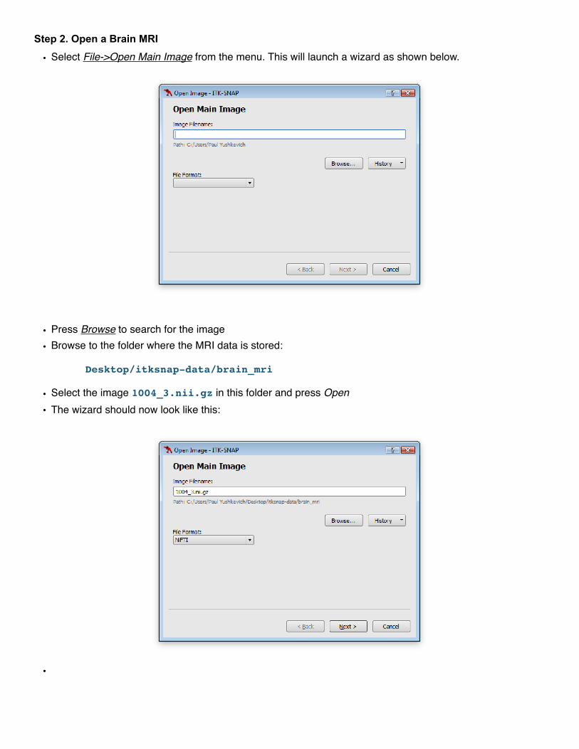
• Press Browse to search for the image• Browse to the folder where the MRI data is stored:

Desktop/itksnap-data/brain_mri

• Select the image 1004_3.nii.gz in this folder and press Open• The wizard should now look like this:

•

• Press Next. The wizard will go to the next page that shows summary information about the image.

�

• Press Finish. ITK-SNAP main window should now show three orthogonal views of a brain MRI scan.

Step 3. Quick Contrast Adjustment

• Open the Layer Inspector (Tools->Layer Inspector or � button on the main toolbar)• Click the Contrast tab• Press Auto to adjust the contrast automatically.

�• Close the Layer Inspector

What are the dimensions of the image you just loaded?

________ by ________ by ________

What are the level and window after automatic con-trast adjustment?

Level: ________ Window: ________

Step 4. Focus in on the Left Hippocampus

• Make sure the Crosshair mode is selected as shown:

• Position the 3D cursor in the middle of the left hippocampus (see illustration below)• You can left-click in any of the three slice views to position the cursor• Or you can hold and drag the left mouse button for faster navigation• Or you can enter cursor position (114,116,110) in the Cursor Inspector panel (highlighted below)

• Now select the Zoom/Pan mode from the main toolbar

• Zoom in on the hippocampus• Hold the right mouse button in one of the slice views and drag up/down to zoom in or out• Or press the 4x button in the Zoom Inspector panel

• Pan in each of the slice views so that the hippocampus is centered in each view• Hold and drag the left mouse button in each slice view until the hippocampus is centered• Or hold and drag the white rectangle in the yellow zoom thumbnail• Or press Center on Cursor in the Zoom Inspector (shortcut C)

Step 5. Fine Contrast Adjustment

• Re-open the Layer Inspector window (shortcut is Ctrl-I)• Change the shape of the contrast curve to optimize contrast between tissues in the hippocampus region.

• Click and drag the curve control points to adjust the shape of the curve• You can add more points with the ‘+’ button

Step 6. Load a Segmentation Image File

• Press Zoom to Fit in the Zoom Inspector to make the whole image visible again (shortcut Ctrl-F)• In the main menu, select Segmentation->Open Segmentation to open a wizard (shortcut Ctrl-O)• In the wizard, open the file 1004_3_seg.nii in the same folder as the brain MRI image• When you complete the wizard, the main ITK-SNAP window will show the segmentation

Step 7. Load Segmentation Label Descriptions

• Select the Crosshair Tool in the Main Toolbar.• Notice that in the Cursor Inspector, under Label Under Cursor, the label is “Label 48”• We will now load a set of label descriptions that have anatomical meaning

• In the main menu, select Segmentation->Import Label Descriptions• In the window that opens, press Browse and select file anat_labels.txt, the press Ok.• Under Label Under Cursor, it should now say “Left Hippocampus”, as below• In the lower left view (3D view) press the update button. You will see a rendering of the brain regions.

Step 8. Compute Volumes and Statistics

• In the main menu, select Segmentation->Volumes and Statistics

�

Step 9. Unload the MRI image

• Close the Volumes and Statistics and Layer Inspector windows (if open)• In the main menu, select File->Close All Images (shortcut Ctrl-Shift-W)• Congratulations! You have completed Exercise 1.

What is the volume of the left hippocampus (label 48)?

________ mm3

What is the average intensity of the left hippocampus?

________

Exercise 2: Manual Segmentation

Learning Objectives After completing this exercise, you will know how to

• Load a DICOM image file • Create and edit segmentation labels • Outline structures of interest with the polygon tool • Edit segmentations with the paintbrush tool • [Optional] Use adaptive paintbrush for computer-aided segmentation

Duration: 15 minutes.

Step 1. Load a body CT scan from a DICOM file

• From the main menu, select File->Open Main Image (shortcut Ctrl-G)• Press Browse, then navigate to the folder below:

Desktop/itksnap-data/Thorax 1CTA_THORACIC…/A Aorta w-c 1.5 B20f 60%

• Select the any file in that folder, e.g., IM-0001-0001.dcm and press Open• The wizard should now look like the image on the left below:

• Notice that the File Format has been automatically set to “DICOM Image Series”

• Press Next. A new screen will appear (above, right).• This screen shows all the DICOM series found in the folder• In this case, there is only one DICOM series found, and it is already selected.

• Press Next to show the summary page• Press Finish to close the wizard

Step 2. [Optional] View Image Information and DICOM Metadata

• Open the Layer Inspector (shortcut Ctrl-I), and select the Info tab (below, left)• This lists basic information about the image, like its size, voxel dimensions, etc.

• Now select the Metadata tab (below, right)• This lists all the information contained in the image header• You can search for specific entries by typing in the Filter field

Step 3. Locate the Spleen

• Use the Crosshair tool to find the spleen (as shown below)

Step 4. Create Anatomical Labels

• In the main menu, select Segmentation->Label Editor (shortcut Ctrl-L)• The label editor should contain seven labels with generic names, as shown below• If it does not (e.g., brain labels from the previous exercise are shown), reset the label list by pressing

Actions button at the bottom of the window, and selecting Reset Label Descriptions

• Select Label 1 in the list on the left• Under Description, type in “Spleen”

• You may also want to change the color for the spleen label• Create additional labels for left and right kidneys, liver, etc.

• Use the New button if you decide to create more than 6 labels• Close the Label Editor window

Step 5. Select the Active Label

• In the Segmentation Labels panel, make sure that “Spleen” is selected as the Active Label.• Also ensure that “All Labels” is selected as the Paint over setting

Step 6. Label the Spleen using the Polygon Tool

• Set the zoom factor to 2x and center the view on the spleen (zoom/pan was covered in Exercise 1)• Select the Polygon Tool in the Main Toolbar

• Using a series of left clicks, draw the outline of the spleen in one of the slice views• Finish drawing by clicking on the first point - the outline will turn red (below, right)

• If you wish to edit the contour, you can click and drag on individual point (below left), or draw an edit box around multiple points (below, middle).

• Once satisfied, press accept, and the contour will be integrated into the segmentation (above, right)• When you hit accept, all the voxels inside of the polygon are assigned the active label (Spleen)• ITK-SNAP represents segmentations by assigning each voxel a unique label

• Draw the spleen outline in other slice views (you won’t have time to segment the entire structure of course, so just do as much as you need to get the hang of the polygon tool)

• Notice that once you accept a polygon in one slice view (e.g., sagittal), it becomes visible in the other slice views (coronal, axial)

• You can also render your partial segmentation in the 3D view by pressing update.

Step 7. Draw small structures using the Paintbrush Tool

• In the Main Toolbar, select the Paintbrush Tool.

• In the Paintbrush Inspector, under Brush Style, select the circle (round brush)• Under Brush Options, check Isotropic

• Hold and drag the left mouse button to paint with the active label (spleen)• Hold and drag the right mouse button to paint with the clear label

Step 8. [Optional] Use the Adaptive Brush Style The adaptive brush style adapts the brush shape based on the image content. It can be used to quickly label parts of structures that are distinctive from surrounding structures

• Open the Label Editor (Ctrl-L) and create a “Lung” label• Select “Lung” as the active label• Position the cursor at coordinate 360, 292, 215

• To do this, you need to select the Crosshairs Mode to access the Cursor Inspector• Select Paintbrush Mode• In the Paintbrush Inspector, under Brush Style, select the last icon (adaptive brush)• Set Brush Size to 40• Click (do not drag) somewhere in the lung, close to other tissues.

• Notice how just the lungs get painted with the lung color, while the surrounding tissue is not.• Changing the granularity and smoothness parameters changes adaptive brush behavior

Step 9. Save your segmentation Segmentations in ITK-SNAP are saved as a special kind of image, where each voxel holds a value referencing an anatomical label.

• From the main menu, select Segmentation->Save Segmentation Image• Select the file format for the segmentation (NIFTI is a good choice) • Assign a filename and hit Finish

• Congratulations, you have finished Exercise 2!

MODULE II: Semi-Automatic Segmentation

Exercise 3: Basic Semi-Automatic Segmentation

Learning Objectives In this exercise, we will use semi-automatic segmentation to label the spleen in the CT image from Exercise 2. After completing this exercise, you will know how to

• Perform semi-automatic segmentation on a single image • Selects regions of interest for semi-automatic segmentation • Use thresholding to pre-segment image into foreground and background • Initialize the active contour using bubbles • Perform contour evolution

Duration: 15 minutes.

Step 1. Open the CT DICOM File from Exercise 2 For this exercise, we will continue working with the same CT dataset as in exercise 2. If you already have it opened, continue to the next step.

• Load the CT image from

Desktop/itksnap-data/Thorax 1CTA_THORACIC…/A Aorta w-c 1.5 B20f 60%

• If you completed Exercise 2, then this image will be in your recent image history. Access it by select-ing from the main menu File->Recent Main Images->[Image Name]

• If you did not complete Exercise 2, see Step 1 in Exercise 2.

Step 2. Unload previous segmentation This step clears the segmentation you created in Exercise 2.

• From the main menu, select Segmentation->Unload Segmentation.• If prompted to save the segmentation, press Discard.

Step 3. Select Region of Interest for Automatic Segmentation This is a preparatory step for semi-automatic segmentation.

• From the main menu, select Edit->View Zoom->Zoom to Fit in All Views (Ctrl-F), which will make the whole CT image visible in all three slice views

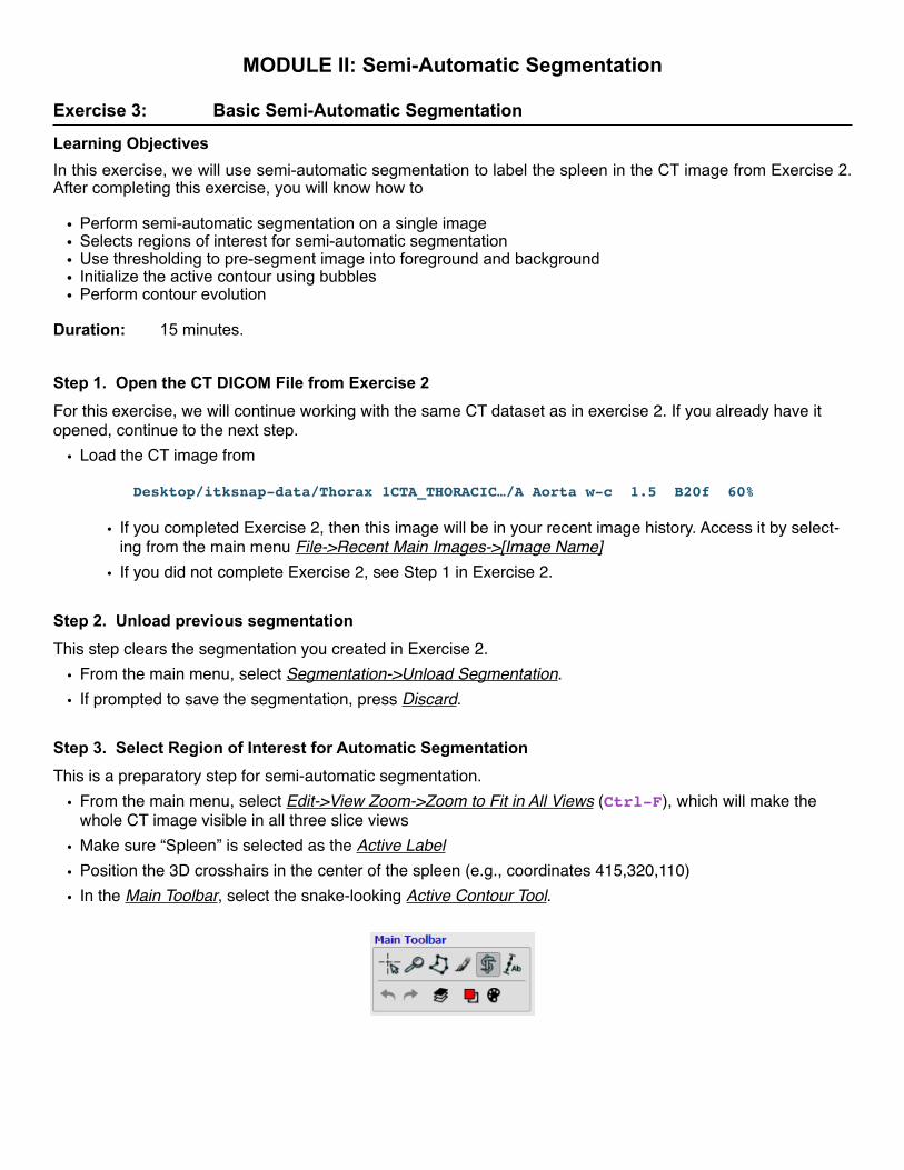
• Make sure “Spleen” is selected as the Active Label • Position the 3D crosshairs in the center of the spleen (e.g., coordinates 415,320,110)• In the Main Toolbar, select the snake-looking Active Contour Tool.

• Using the left mouse button, drag the corners of the red selection box, so that the box encompasses the spleen, as shown below

• Or you can type in the position (300,209,47) and size (194,216,118) of the selection box in the Snake Inspector, as highlighted below

• Press Segment 3D to enter the semi-automatic segmentation mode.

Step 4. Use Thresholding to Isolate the Spleen

• Your ITK-SNAP window should look like the screenshot below. Each slide view will show two images side by side. On the left is the region of interest of the CT, and on the right is the so-called speed image, which should be white in spleen voxels, and blue in non-spleen voxels.

• If your images are now shown side by side, press the little button � in the right top corner of any of the three slice views

• If the CT image contrast looks wrong, select from the main menu Tools->Image Contrast->Auto Adjust Contrast (Ctrl-J).

• In the tool panel on the right hand side of the ITK-SNAP window, ensure that under Actions, the Preseg-mentation Mode is set to “Thresholding”

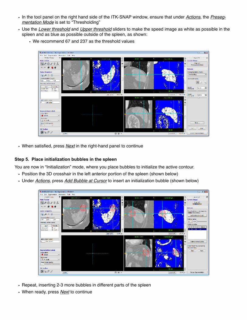
• Use the Lower threshold and Upper threshold sliders to make the speed image as white as possible in the spleen and as blue as possible outside of the spleen, as shown:

• We recommend 67 and 237 as the threshold values

• When satisfied, press Next in the right-hand panel to continue

Step 5. Place initialization bubbles in the spleen You are now in “Initialization” mode, where you place bubbles to initialize the active contour.

• Position the 3D crosshair in the left anterior portion of the spleen (shown below)• Under Actions, press Add Bubble at Cursor to insert an initialization bubble (shown below)

• Repeat, inserting 2-3 more bubbles in different parts of the spleen• When ready, press Next to continue

Step 6. Run active contour segmentation You are now in “Evolution” mode, where you let the bubbles grow to fill the spleen.

• In the 3D visualization panel (lower right quadrant), press update to visualize the bubbles

• Under Actions, press the play button (� ) to start evolution.• As the contour evolves, you can press update in the 3D visualization panel to get a rendering

• After about 350 iterations, press the pause button (� ) under Actions to stop evolution

• If you are not satisfied with the segmentation, you may press the Back button to return to the pre segmen-tation and initialization stages, and use different threshold values or bubble placement.

Step 7. [Optional] Repeat segmentation with different parameters To obtain a smoother spleen segmentation, we can change the parameter that controls smoothness.

• Under Actions, press Set Parameters button• In the window that opens (see below), set a larger (0.8) value of the Smoothing (curvature) force,

• Press Close to close the window.

• Rewind the segmentation (� ), and run again for 350 iterations.

Step 8. Exit semi-automatic segmentation mode

• Under Actions, press the Finish button. Your segmentation of the spleen will be integrated into the overall segmentation of the CT image.

• You can now repeat this process for various other structures in the CT scan

• Congratulations, you completed Exercise 8!

Exercise 4: Multi-Modality Semi-Automatic Segmentation

Learning Objectives In this exercise, we will use semi-automatic segmentation to label a brain tumor from multiple MRI contrasts of the same subject.

• Open ITK-SNAP workspaces • Work with multiple images at once • Use the “classification” pre-segmentation mode to generate speed images

Duration: 15 minutes.

Step 1. Open an ITK-SNAP workspace with multiple image files

• From the main menu, select Workspace->Open Workspace.• If prompted to save unsaved changes, press Discard.• In the Open Workspace dialog window (below), press Browse

• Locate the workspace file for this exercise:

Desktop/itksnap-data/VSD.Brain.54513/VSD.Brain.54513.itksnap

• Press Open to open the workspace. Your screen will look like one of the images below:

• The layout on the left is called “Tiled layout” and the layout on the right is “Thumbnail layout”.

• Toggle between these layouts using the buttons � and � on the top right area of each slice panel

Step 2. Experiment with the Thumbnail layout

• Enter the “Thumbnail layout” by pressing the � button in one of the slice panels• Press on the thumbnails on the right hand side of each slice view to select the different MRI contrasts• When your mouse is over a thumbnail, you will see a small round button appear. Press it to reveal a con-

test many for that image.

• Use the context menu to adjust the contrast and color map of the different images. • Or press Ctrl-J to auto-adjust contrast in all images

Step 3. Select the Region of Interest for Tumor segmentation

• In the Main Toolbar, select the snake-looking Active Contour Tool.• The region of interest will become visible. It is predefined in the workspace file that you loaded.

• [Optional] check that the tumor is included in the region of interest for all modalities. Do do this, for each modality take turns selecting it, and then scroll through the different image slices to make sure the tumor and surrounding edema are in the region of interest. Adjust the region if needed.

• Press Segment 3D to enter semi-automatic segmentation mode

Step 4. Pre-segmentation using classification In this step, instead of thresholding used in Exercise 2, we will provide ITK-SNAP with examples of different tissue types in the image.

• Under Actions, set Presegmentation Mode to “Classification”• The panel will look like what is shown on the right

• Hover the mouse over the little color buttons in the panel. You will see that each one corresponds to an anatomical label.

• Pressing the colored buttons will select set its label as the Active label and will also select the Paintbrush tool in the Main Toolbar.

• Using the buttons, paint examples of each tissue class in the image.• The contrast-enhanced “T1ce” image (second thumbnail) is best suited for

labeling examples of the tumor core and enhancing tumor.• The FLAIR image is good for drawing examples of edema

• The adaptive paintbrush � is helpful for drawing examples of the enhanc-ing part of the tumor, which is thin.

• See examples below of progressive labeling of tumor core, enhancing tumor, edema, normal brain, and other (fluid, non-brain region)

• It is easiest to draw all your examples on just one slice, as we did below

• Press Train Classifier.• Press the thumbnail for the speed image. Your window should look like what you see below.

• Press on different labels listed in the Foreground class(es) box. For each class you click on, a different speed image will appear.

• Flip between the speed image and the different MRI images. If you think the speed image is incorrect, you can edit your examples and train the classifier again

• Now, using Shift-click to select both “Tumor Core” and “Enhancing Tumor” in the Foreground class(es) box

• The reason we do this is that it is easier to first segment the two parts of the tumor together and then separate out the tumor core, than to segment the thin narrow enhancing tumor region independently.

• Select “Enhancing Tumor” as the active label (left panel, Segmentation Labels)• Press Next in the right panel.

Step 5. Perform Active Contour Segmentation

• Place a single bubble in the bright region of the speed image.• Press Next

• Run the segmentation as you did in Exercise 3.

• Press finish to send the segmentation into the main ITK-SNAP window.

Step 6. Repeat segmentation for the tumor core

• In the Main Toolbar, select the snake-looking Active Contour Tool, and press Segment 3D.• Notice how the examples you previously drew are still there

• Select “Tumor Core” in the Foreground classes box• Important: Select “Tumor Core” as the active label• Perform segmentation of the tumor core as in Step 5.• When you finish, the segmentation should look like this

Step 7. Repeat segmentation for the edema

• Follow the same sequence of steps to label edema

Conclusions

By now, you have discovered the most widely used features of ITK-SNAP. The combination of semi-automatic and manual segmentation tools you have used should make it possible to solve a broad range of segmentation problems using ITK-SNAP.

There are several additional tools and functionalities that ITK-SNAP provides. We did not have time to cover all of them in these exercises, and we invite you to explore them on your own. These features include:

• Using the 3D editing tools like the 3D scalpel• Using different color maps to display images• Displaying images (e.g., statistical maps) as overlays on top of other images• Saving screenshots• Exporting segmentations as surface meshes, e.g., for 3D printing• Additional pre-segmentation modes (edge-based and clustering-based)• Annotation mode, used to draw lines, measure lengths, and add comments to images• Working with multiple ITK-SNAP sessions at once

Where to Find More Information?

Almost every button, checkbox, and control in ITK-SNAP has a tool tip. Hold your mouse cursor over the but-ton for a second or two, and a tooltip will appear. Using these tooltips is one of the best ways to discover new features.

The itksnap.org website is a source of additional information. Through the website you can find:

• Video tutorials from a day-long training course• Discussion boards for ITK-SNAP users and developers• Information on the companion image processing tool Convert3D