284-2009: The Basics of Experimental Design for...

Paper 284-2009

The Basics of Experimental Design for Multivariate Analysis Steve Figard, Abbott Laboratories, Abbott Park, IL

ABSTRACT This paper is designed for the beginner to intermediate practitioner of the form of analysis known as Design of Experiments (DOE). Specific objectives include:

• Defining some of the terminology • Introducing major thought processes, philosophy, strategies, and rules of thumb • Keeping objectives in the context of JMP® as an example of how this type of analysis is implemented in

software • Presenting a relevant example of the use of DOE in assay development

Letting the software worry about the how of DOE, this paper focuses on the when and why to do what. ALTERNATE TITLES

How to Vary More Than One Variable at a Time & Still Survive Your Audit INTRODUCTION The programmers at the SAS Institute have labored long and hard to beef up the DOE module for JMP as the version number has increased. In response to this effort, a primary objective of this paper is to answer the question, “Why should I pay any attention to the DOE module in JMP?” Or perhaps in other words, “What’s in DOE for me?” SAS documentation and training is one excellent way to both learn the software and the methodology, but here we will focus on some of the ideas not covered in that material as an introduction to the concept of DOE. WHAT IS DOE? DOE is an acronym for Design of Experiments, a collection of techniques sometimes known amongst statisticians as “multivariate experimental design and analysis.” In somewhat plainer English, it is a methodology which allows the experimenter to systematically vary multiple factors within the context of one experimental design, and use the results to create mathematical models of the process being examined. Using these models, it is then possible to find the true optimum of a process, accounting for interactions and revealing the most important inputs into that process. This is in distinct contrast to the time honored tradition approach of one-factor-at-a-time.

“Statistical analysis: Mysterious, sometimes bizarre, manipulations performed upon the collected data of an experiment in order to obscure the fact that the results have no generalizable meaning for humanity. Commonly, computers are used, lending an additional aura of unreality to the proceedings.” · Author Unknown

OFAT OFAT is another acronym frequently seen in this context, and does not refer to how one answers the wife’s question regarding how her new dress makes her look! As concluded in the previous section, OFAT, or one-factor-at-a-time, is the guiding principle of the scientific method, especially when investigating the unknown. In such cases, it is the method of choice. However, when you know the input factors for a given process, and have an approximation of the values for those inputs that yield acceptable final product, OFAT fails to give you any information about interactions and consequently frequently results in finding secondary optima rather than the true optimum set of conditions for your process. In addition, the statistical power of OFAT is considerable less than DOE and the ability to predict results when inputs vary is totally absent from OFAT. As an example of how OFAT works (or doesn’t work well, depending on your viewpoint), consider the situation of a process with two input variables. With OFAT, the investigator chooses a fixed setting for one input variable and finds the optimum for the second variable. As a second step, the second variable is fixed at this alleged optimum and now the first variable is investigated and the optimum found for it. In so doing, the alleged optimum for the process is (sometimes) found. In situations where there is an interaction between the two input variables, the possibility of finding a secondary optimum and not the true optimum of the process increases greatly. In more complex cases where there are more than two input factors under investigation, the situation rapidly becomes unmanageable. Moreover, since the presence of the interaction is not revealed by OFAT, should problems arise in the future when natural variation leads to a shift in the input factors, there is no true characterization of the process thus minimizing the probability of finding a solution.

“Prediction is very hard, especially when it is about the future.” · Yogi Berra

1

SAS Presents... JMPSAS Global Forum 2009

THE SPECIFIC GOALS OF DOE The specific goals of DOE are those which truly cannot be easily accomplished by OFAT, and all revolve around characterizing to a high degree the process under investigation. The first goal is to identify critical parameters for further study, while eliminating those whose impact is minimal or totally insubstantial. The second is to predict the performance of your process in a robust (reproducible) fashion. The overarching goal of both of these is to do so with the minimum use of resources, both time and equipment/reagents, operationally defined as the smallest number of experimental trials that will give you meaningful data for analysis. At this point, it should be emphasized that DOE is not a panacea for shortcomings in your experimental situation. It is a tool, and as any other tool, has its appropriate and inappropriate use. One must know how and when to use it. That said, it is a very powerful tool when used properly. “[Don’t] use statistics as a drunken man uses lamp posts, for support

rather than illumination.” ·Andrew Lang

THE LOGICAL FLOW OF DOE When DOE was defined, an adjective used was “systematic.” This suggests a logical flow to the methodology, and that flow may be summarized in the following bullet points:

• State & document objectives • Select variables/factors & models to support the objective • Create a design to support the model • Collect the data based on the design • Execute the analysis with the software • Verify the model with check points • Report: if it ain’t documented, signed and witnessed, you never done it!

The remainder of this paper will expand upon each of these steps with some details, and then an example of DOE in use will be examined. OBJECTIVES Someone has aptly said that if you aim for nothing, you are bound to hit it. Thus, it is crucial at the outset to have a clear picture of what you need to accomplish with the experiments you are planning. There are two distinct goals for DOE that call for two distinct types of designs.

The first is simply to identify critical factors. This is called a SCREENING design and is accomplished with a simpler surface to allow the evaluation of a larger number of possible factors. The idea is to first find out which

factors have no impact on the final outcome of the process and thus can be ignored, or which have minimal impact on the final outcome and so can be fixed at values convenient to the purpose of the experimenter.

“It’s better to solve the right problem approximately than to solve the wrong problem exactly.” ·J. W. Tukey

Once the critical factors which clearly have the greatest impact on the process have been identified, a RESPONSE SURFACE design (sometimes known as RSM, for Response Surface Method) will be used to characterize the response relative to these input factors. Here the objective is to construct a model to predict process outcomes based on the input at various settings of the critical factors. A model so constructed should also allow true optimization of the process. Should the ultimate goals of the process change over time, the model in hand should then allow re-optimization. Because fewer factors are evaluated, a more complex surface design can be used for RSM experiments. In cases where the process is simple enough, a Screening design can also be predictive. Fortunately, reality is not always complex. The software should give diagnostics to allow the experimenter to determine whether or not this is so. FACTORS (VARIABLES) The factors in an experiment also fall into two categories: input or design factors, and output or response factors. The input factors are the independent control variables, essentially the knobs you turn to adjust your output. They are the settings that define your process, and can be continuous, categorical, mixture, or blocking. Continuous factors are measured on a continuous scale, such as temperature, and thus can have fractional values, such as 23.45. Categorical variables, in contrast, are discrete units, such as instrument, or building, or test site. (You would have a difficult time executing an experiment with 2.5 instruments!) Categorical variables increase the size and complexity of the design and analysis and this should be kept in mind when planning, especially if resources are limited. These first two categories are the ones most frequently encountered.

2


Mixture factors are a special class of continuous factors measured in proportions which must all add up to 100%. They can appear in processes in which there are fixed manufacturing capacities of, for example, volume. The reaction vessel can hold 100 liters of fluid and there are three fluids to be combined to make your product. The optimum mixture of these three components would be a mixture design with mixture variables. This particular design and analysis is outside the scope of this paper, but JMP can handle it and so I mention it here for completeness. Lastly, blocking variables are a special type of categorical variable used to account for known sources of variation that are not really part of the experiment but are caused by changes in personnel, materials, or machinery, or by the fact that you can’t complete all your runs on one day. The specifics of dealing with blocking variables are left to the reader to determine and again, JMP can handle these types of variables. Here is one of the places that “the art” of DOE enters the picture: the accurate selection of the factors to be included as input and output for the study. The reason is simple: most processes have many potential input factors influencing the output. Prior knowledge of the process or of similar processes must be applied where available to weed out the factors to a reasonable number even for a screening design. If it is possible to avoid categorical variables, do so.

“You know my method. It is founded upon the observation of trifles.” ·Sherlock Holmes, The Boscombe Valley Mystery

MODELS The model is a mathematical construct, i.e., formula, inferred from the collected data using statistical methods. It ties together the response and control factors and defines the possible shape of the response surface. The more complex the model, the more data will be required to define the model. Thus, it is better to create a design based on a more complex model, but then analyze with a simpler model. You cannot, however, run a design of a simpler model and analyze the results with a more complex model. There will be insufficient data to do so. This will be discussed in greater detail in the next section on Designs. Here, you must be careful not to adopt a model that describes the noise of a process. This situation is usually found when the correlation coefficient is at or very near perfect (1.000). Measurement error, indeed, human error, should lower this metric away from perfection. Thus, if a complex model results in correlation coefficients of approximately one, you should suspect you are modeling the noise along with the data. By way of illustration, I will now illustrate the way models define certain shapes.

• Figure 1: Line: Linear model in 1 variable o y = a + bx o slope in x direction o no slope in z direction o line for z = 0

3


• Figure 2: Plane: Linear Model in 2 Variables o y = a + bx + cz o Used to analyze screening designs o No curvature o No interactions o x and z are “Main Effects”

• Figure 3: Interaction Twists Plane o y = a + bx + cz + dxz o Still no curvature

• Figure 4: Interaction & Curvature in x Variable Only o y = a + bx + cz + dxz + ex2

4


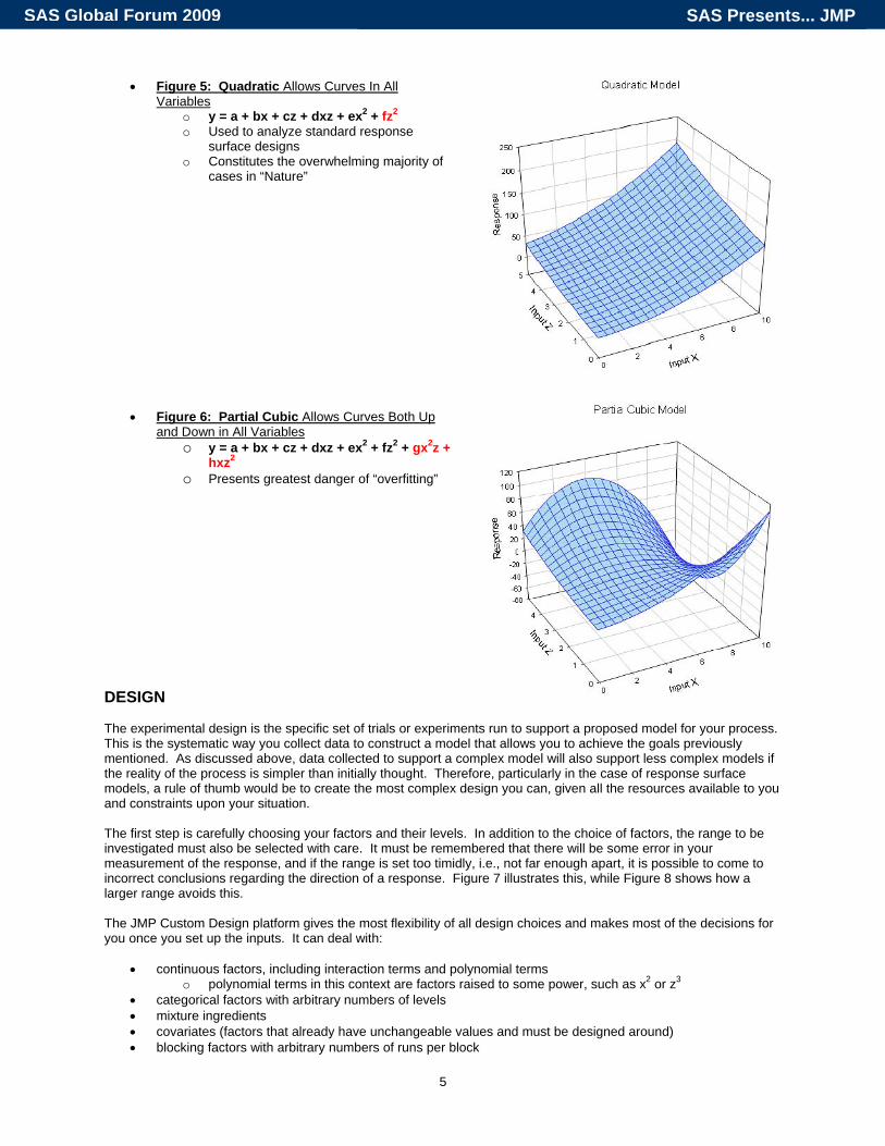
• Figure 5: Quadratic Allows Curves In All Variables

o y = a + bx + cz + dxz + ex2 + fz2 o Used to analyze standard response

surface designs o Constitutes the overwhelming majority of

cases in “Nature”

• Figure 6: Partial Cubic Allows Curves Both Up and Down in All Variables

o y = a + bx + cz + dxz + ex2 + fz2 + gx2z + hxz2

o Presents greatest danger of “overfitting” DESIGN The experimental design is the specific set of trials or experiments run to support a proposed model for your process. This is the systematic way you collect data to construct a model that allows you to achieve the goals previously mentioned. As discussed above, data collected to support a complex model will also support less complex models if the reality of the process is simpler than initially thought. Therefore, particularly in the case of response surface models, a rule of thumb would be to create the most complex design you can, given all the resources available to you and constraints upon your situation. The first step is carefully choosing your factors and their levels. In addition to the choice of factors, the range to be investigated must also be selected with care. It must be remembered that there will be some error in your measurement of the response, and if the range is set too timidly, i.e., not far enough apart, it is possible to come to incorrect conclusions regarding the direction of a response. Figure 7 illustrates this, while Figure 8 shows how a larger range avoids this. The JMP Custom Design platform gives the most flexibility of all design choices and makes most of the decisions for you once you set up the inputs. It can deal with:

• continuous factors, including interaction terms and polynomial terms o polynomial terms in this context are factors raised to some power, such as x2 or z3

• categorical factors with arbitrary numbers of levels • mixture ingredients • covariates (factors that already have unchangeable values and must be designed around) • blocking factors with arbitrary numbers of runs per block

5


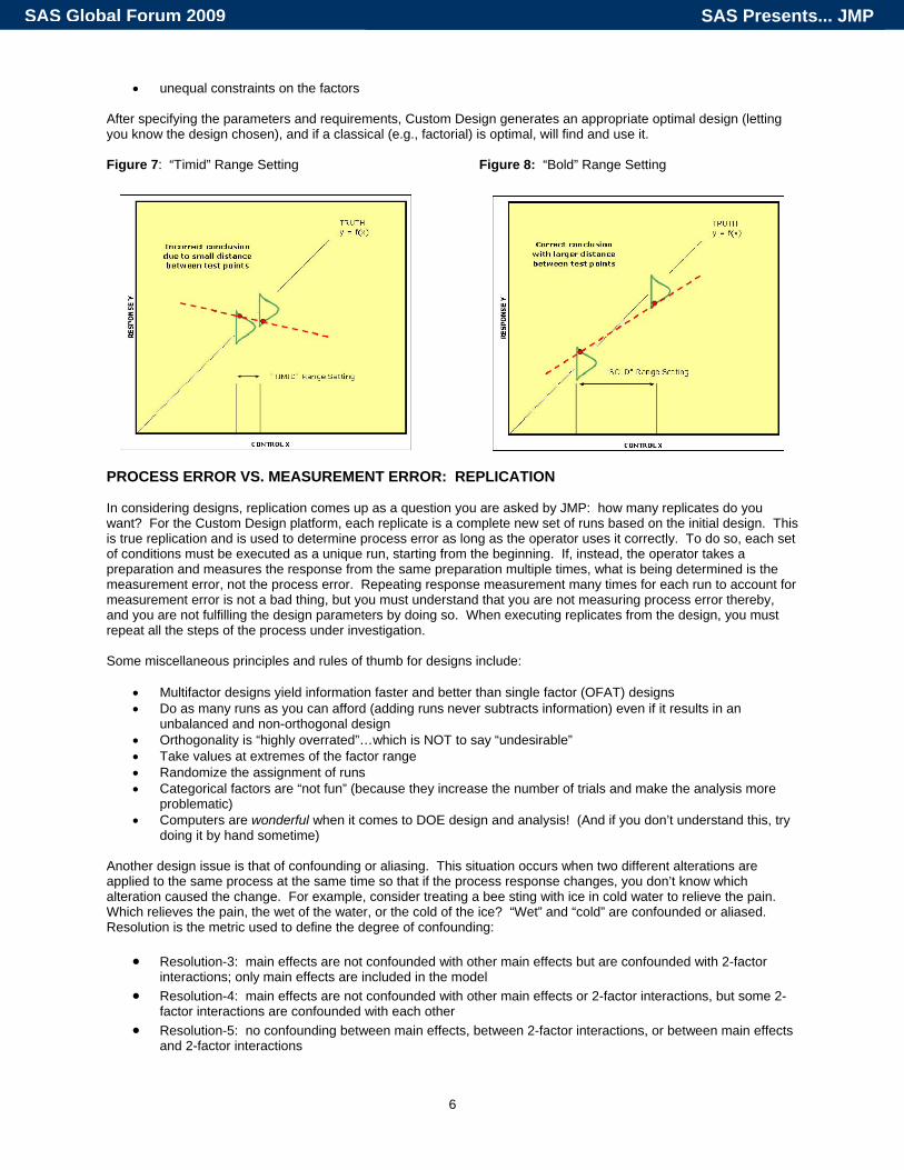
• unequal constraints on the factors After specifying the parameters and requirements, Custom Design generates an appropriate optimal design (letting you know the design chosen), and if a classical (e.g., factorial) is optimal, will find and use it. Figure 7: “Timid” Range Setting Figure 8: “Bold” Range Setting

PROCESS ERROR VS. MEASUREMENT ERROR: REPLICATION In considering designs, replication comes up as a question you are asked by JMP: how many replicates do you want? For the Custom Design platform, each replicate is a complete new set of runs based on the initial design. This is true replication and is used to determine process error as long as the operator uses it correctly. To do so, each set of conditions must be executed as a unique run, starting from the beginning. If, instead, the operator takes a preparation and measures the response from the same preparation multiple times, what is being determined is the measurement error, not the process error. Repeating response measurement many times for each run to account for measurement error is not a bad thing, but you must understand that you are not measuring process error thereby, and you are not fulfilling the design parameters by doing so. When executing replicates from the design, you must repeat all the steps of the process under investigation. Some miscellaneous principles and rules of thumb for designs include:

• Multifactor designs yield information faster and better than single factor (OFAT) designs • Do as many runs as you can afford (adding runs never subtracts information) even if it results in an

unbalanced and non-orthogonal design • Orthogonality is “highly overrated”…which is NOT to say “undesirable” • Take values at extremes of the factor range • Randomize the assignment of runs • Categorical factors are “not fun” (because they increase the number of trials and make the analysis more

problematic) • Computers are wonderful when it comes to DOE design and analysis! (And if you don’t understand this, try

doing it by hand sometime) Another design issue is that of confounding or aliasing. This situation occurs when two different alterations are applied to the same process at the same time so that if the process response changes, you don’t know which alteration caused the change. For example, consider treating a bee sting with ice in cold water to relieve the pain. Which relieves the pain, the wet of the water, or the cold of the ice? “Wet” and “cold” are confounded or aliased. Resolution is the metric used to define the degree of confounding:

• Resolution-3: main effects are not confounded with other main effects but are confounded with 2-factor interactions; only main effects are included in the model

• Resolution-4: main effects are not confounded with other main effects or 2-factor interactions, but some 2-factor interactions are confounded with each other

• Resolution-5: no confounding between main effects, between 2-factor interactions, or between main effects and 2-factor interactions

6


Finally, the DOE literature is replete with design names, a detailed description of each being beyond the scope of this paper. Classical designs available in JMP include factorial, fractional factorial, Plackett-Burman, and Taguchi designs. Two newer designs that the Custom Design platform may select for you are the D-optimal and the I-optimal. The D-optimal design maximizes a criterion so that you learn the most about the parameters and is particularly useful for screening designs. In contrast, the I-optimal design maximizes a criterion so that the model predicts best over the region of interest, rendering this design particularly useful for response surface optimization. DATA COLLECTION There are a few rules of thumb regarding the collection of the data once the design has been determined. First, get involved in the data collection if you aren’t doing it yourself. Communicate the why and how you are doing things and engage all your people skills to create an atmosphere of teamwork. Share the ownership of the design, the experiment, and the entire problem solving or characterization endeavor. Your output will only be as good as your input, and you want people filling in the results based on actual observations, not what they “know” the result will be based on their experience or how it’s always been done. As someone has aptly said, don’t risk your career on “delivered” data.

“There is nothing like first-hand evidence.” ·Sherlock Holmes, A Study in Scarlet

Secondly, to reinforce a previously mentioned point, randomize the order in which the trials are run whenever possible to break correlations between the studied control variables and the unknown variables.

“Get your facts first, and then you can distort them as much as you please. (Facts are stubborn, but statistics are more pliable.)” ·Mark Twain

ANALYSIS This step is simply the creation from your data of a specific mathematical model defining the behavior of your specific process. Keeping in mind that the ultimate goal is to predict the response for any given settings of the input control variables, the analysis must answer two initial questions:

1. Does the model fit the data? (If the model does not fit the data, its utility is limited at best.) 2. What are the important factors/variables?

If the experiment follows a screening design, then the important factors should be carried over to a response surface experiment. If it is already a response surface experiment, the important factors should be used as axes for contour plots and provide the focus of attention in the JMP Profiler tools. Analysis of DOE data in JMP is done in the Analyze > Fit Model submenu. JMP tutorials provide the necessary instructions for the actual execution and I will not duplicate that material here. Tools and metrics to consider include (but are not limited to):

• p-values for the ANOVA and for individual factors, a metric for identifying important factors • R square: rule of thumb ≈ % of the data accounted for by the factors in the model, in addition to being a

metric for how well the model fits the data • R square adjusted: adjusts the R square value to make it more comparable over models with different

numbers of parameters by using the degrees of freedom in its computation • Normal Plot: significant (important) factors appear as outliers that lie away from the line that represents

Normal noise and helpfully labeled for you by JMP • Profiler tools: see JMP documentation for details (we will look at the Prediction Profiler later)

o Prediction Profiler o Interaction Profiler o Contour Profiler

MODEL VERIFICATION It is critical to always, always, ALWAYS check the model’s ability to predict before implementing those predictions in mass production of final product. Such verification runs are sometimes called check points, trials run after the analysis at settings not used to create the model to verify said model’s accuracy and proximity to reality. Check points should be done at certain input settings such as:

• near the process optimum • near suspicious behavior • at low cost settings • inside versus outside the range of experiments

7


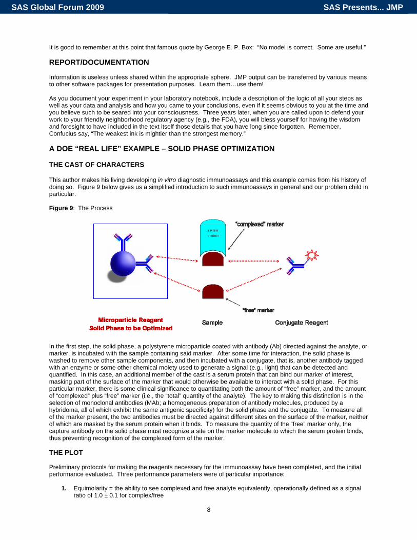
It is good to remember at this point that famous quote by George E. P. Box: “No model is correct. Some are useful.” REPORT/DOCUMENTATION Information is useless unless shared within the appropriate sphere. JMP output can be transferred by various means to other software packages for presentation purposes. Learn them…use them! As you document your experiment in your laboratory notebook, include a description of the logic of all your steps as well as your data and analysis and how you came to your conclusions, even if it seems obvious to you at the time and you believe such to be seared into your consciousness. Three years later, when you are called upon to defend your work to your friendly neighborhood regulatory agency (e.g., the FDA), you will bless yourself for having the wisdom and foresight to have included in the text itself those details that you have long since forgotten. Remember, Confucius say, “The weakest ink is mightier than the strongest memory.” A DOE “REAL LIFE” EXAMPLE – SOLID PHASE OPTIMIZATION THE CAST OF CHARACTERS This author makes his living developing in vitro diagnostic immunoassays and this example comes from his history of doing so. Figure 9 below gives us a simplified introduction to such immunoassays in general and our problem child in particular. Figure 9: The Process

In the first step, the solid phase, a polystyrene microparticle coated with antibody (Ab) directed against the analyte, or marker, is incubated with the sample containing said marker. After some time for interaction, the solid phase is washed to remove other sample components, and then incubated with a conjugate, that is, another antibody tagged with an enzyme or some other chemical moiety used to generate a signal (e.g., light) that can be detected and quantified. In this case, an additional member of the cast is a serum protein that can bind our marker of interest, masking part of the surface of the marker that would otherwise be available to interact with a solid phase. For this particular marker, there is some clinical significance to quantitating both the amount of “free” marker, and the amount of “complexed” plus “free” marker (i.e., the “total” quantity of the analyte). The key to making this distinction is in the selection of monoclonal antibodies (MAb; a homogeneous preparation of antibody molecules, produced by a hybridoma, all of which exhibit the same antigenic specificity) for the solid phase and the conjugate. To measure all of the marker present, the two antibodies must be directed against different sites on the surface of the marker, neither of which are masked by the serum protein when it binds. To measure the quantity of the “free” marker only, the capture antibody on the solid phase must recognize a site on the marker molecule to which the serum protein binds, thus preventing recognition of the complexed form of the marker. THE PLOT Preliminary protocols for making the reagents necessary for the immunoassay have been completed, and the initial performance evaluated. Three performance parameters were of particular importance:

1. Equimolarity = the ability to see complexed and free analyte equivalently, operationally defined as a signal ratio of 1.0 ± 0.1 for complex/free

8


2. Microparticle stability, defined as 100 ± 10% of 2-8ºC signal after 3 days storage at 45ºC 3. Panel values = within 5% of target values across the dynamic range of the assay

The performance in the initial evaluate showed that panel values were within the specified goal, but the microparticles were not stable (signal loss greater than 10%) and the equimolarity performance was marginal. Thus, the experimental objective is to determine a manufacturing formula to meet all three of the above goals. Additional investigations had shown that the loss in stability was related to free antibody coming off of the solid phase during storage as a function of time, suggesting a lack of covalent coupling of the antibody to the microparticles. Dropping the antibody concentration for coating improved the stability, but then the panel values read lower than acceptable, and equimolarity, already marginal, departed further from the target. THE FACTORS Four input factors to the microparticle manufacturing process were evaluated. The first three are the obvious “active ingredients” for the coupling process: the concentration of the coating antibody (in mg/mL), the concentration of the microparticles (in % solids), and the concentration of the coupling reagent, affectionately known as EDAC (a carbodiimide, for those chemically curious, in mg/mL). The fourth factor is the concentration of sodium chloride in mM. Ionic strength is known to impact the interaction of proteins with surfaces, and the concentration of NaCl is one easy way of manipulating this characteristic of the coupling reaction. We already know the three critical output factors in which we have interest. Equimolarity is a simple ratio with a target of one. Panel values were evaluated with a high and a low panel, so this output consists of two ratios (panel value - target value/target value) with a target of zero (zero difference from standards). Stability is evaluated by averaging across calibrators (Cal B-F) and calculating the ratio of (heat stressed – cold storage)/cold storage with the target again zero difference from cold stored calibrators. THE DESIGN A screening design was chosen first to minimize the number of runs and determine the most important factors. Table 1 shows the inputs, and Table 2 shows the design that was run (a screening design: 4 factors, 2 levels with midpoint: 11 unique preps including 5 duplicate preps for a total of 16): TABLE 1: Design Inputs

Factor Low Level High Level Midpoint Current[Ab], mg/mL 0.02 1.0 0.51 2.0[EDAC], mg/mL 0.1 5.0 2.55 1.0[NaCl], mM 0.0 500 250 0.0% solids 0.5 2.0 1.25 1.0

TABLE 2: Design

Pattern Trial # Ab mg/mL EDAC mg/mL NaCl mM % Solids+−++ 1 1 0.1 500 2−+−− 2 0.02 5 0 0.5−+++ 3 0.02 5 500 2+−−− 4 1 0.1 0 0.5+++− 5 1 5 500 0.5−−−+ 6 0.02 0.1 0 2++−+ 7 1 5 0 2−−+− 8 0.02 0.1 500 0.5++++ 9 1 5 500 2−−−− 10 0.02 0.1 0 0.50000 11 0.51 2.55 250 1.25

+−++ 1 1 0.1 500 2−+−− 2 0.02 5 0 0.5−+++ 3 0.02 5 500 2+−−− 4 1 0.1 0 0.5+++− 5 1 5 500 0.5

Note: For the “Pattern” in the above table, low, midpoint, and high settings are shown as minus, zero, and plus signs.

9


THE RESULTS WITH CHECKPOINTS One of the first diagnostics of fit is the plot of predicted versus actual values. The R squared values give an objective measure of that fit, while the plots give a good visual indication of outliers and the overall fit. R square values do not have to be close to one for the model to have predictive power, which is why looking at the plot is helpful in making the decision whether or not to use the model predictions for next steps. Figures 10 and 11 show these results for the two panels. Figures 12 shows the measure of stability used, and figure 13, the equimolarity results. Figure 10: Panel C Predicted vs. Actual Figure 11: Panel I Predicted vs. Actual

Figure 12: Cal B-F Stability Predicted vs. Actual Figure 13: Equimolarity Predicted vs. Actual

These plots show a reasonable ability to predict these responses of interest, with most R Square values above 0.80. Thus, it was decided to attempt optimization using these results first for stability. To do this, we turn to the Prediction Profiler tool (Figure 14). With this tool, the inputs are plotted separately along the x-axes with the range of values used in the design. On the far right is the Desirability function used to optimize the responses (see the JMP tutorial materials for instructions on how to use this plot). The y-axes are the outputs. Plotted this way, you can immediately see visually the impact of each input on each output and verify with your eyes what the p-values and other statistics have told you about your process. For example, we see immediately that the % solids have little influence in any of the responses here. Of particular relevance here is the flat line for the Desirability function for the panels and the equimolarity responses. This is because the target is not on the y-axes for these responses, indicating that the input factors cannot be adjusted to any setting within these ranges that will yield the desired response.

10


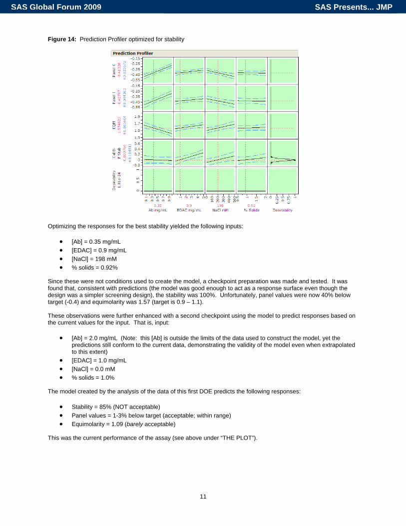
Figure 14: Prediction Profiler optimized for stability

Optimizing the responses for the best stability yielded the following inputs:

• [Ab] = 0.35 mg/mL • [EDAC] = 0.9 mg/mL • [NaCl] = 198 mM • % solids = 0.92%

Since these were not conditions used to create the model, a checkpoint preparation was made and tested. It was found that, consistent with predictions (the model was good enough to act as a response surface even though the design was a simpler screening design), the stability was 100%. Unfortunately, panel values were now 40% below target (-0.4) and equimolarity was 1.57 (target is 0.9 – 1.1). These observations were further enhanced with a second checkpoint using the model to predict responses based on the current values for the input. That is, input:

• [Ab] = 2.0 mg/mL (Note: this [Ab] is outside the limits of the data used to construct the model, yet the predictions still conform to the current data, demonstrating the validity of the model even when extrapolated to this extent)

• [EDAC] = 1.0 mg/mL • [NaCl] = 0.0 mM • % solids = 1.0%

The model created by the analysis of the data of this first DOE predicts the following responses:

• Stability = 85% (NOT acceptable) • Panel values = 1-3% below target (acceptable; within range) • Equimolarity = 1.09 (barely acceptable)

This was the current performance of the assay (see above under “THE PLOT”).

11


The conclusion of this first DOE analysis provides an important lesson on the utility of DOE. The four inputs studied here do not provide a means to simultaneously optimize stability, equimolarity, and panel values. To do so, you must either a.) accept a tradeoff in response outputs, i.e., change the design goals (which is not a good idea if those design goals have been properly formulated from customer requirements), or b.) entertain a new perturbation/parameter in the assay system, i.e., look at something new, a different parameter not yet evaluated, or something radically new to the entire system. A CRITICAL ADVANTAGE OF USING DOE “Lack of Success” is not the same as “Failure.” One of the greatest benefits of DOE is the ability to terminate unfruitful lines of investigation using the objective evidence of the validated models generated to scientifically justify this decision. This occurs when the model predictions have been verified (validating the model) and when those predictions show the impossibility of meeting all necessary goals simultaneously.

“Eliminate all other factors, and the one which remains must be the truth.” ·Sherlock Holmes, The Sign of the Four

WHAT TO DO? At this point, a preliminary experiment done months earlier surfaced again, suggesting a new direction to evaluate in earnest. At the time, it was set aside as “interesting results” having no practical utility. At that time it was observed that if you added the monoclonal Ab (MAb) against the free marker to the solid phase diluent to create a pseudo-complexed marker from the free marker, all forms of the marker appeared to look alike in the “total” assay. This addresses the panel values and the equimolarity issue. The new hypothesis, therefore, was, can we optimize the solid phase coating for stability and then adjust the panel values and equimolarity results with this MAb in the diluent? THE FACTORS & DESIGN, PART 2 Based on the first DOE the % solids and NaCl concentrations were fixed and dropped from this study, leaving only three factors: TABLE 3: Design Inputs

Factor Low Level High Level Midpoint Current[Ab], mg/mL 0.05 1.0 0.525 1.0[EDAC], mg/mL 0.5 10.0 5.25 2.5[Mab in diluent], mg/mL 0.10 2.0 1.05 0.0

With fewer factors to evaluate, and a stronger need to create a model that would be predictive, a D-optimal RSM with 3 factors, 3 levels, and 5 duplicate reps was designed and executed. TABLE 4: Design

Pattern Trial # Ab mg/mL EDAC mg/mL [MAb] mg/mL in diluent

-++ 1 0.05 10 2.0+0- 2 1.0 5.25 0.1-+- 3 0.05 10 0.1--+ 4 0.05 0.5 2.0

+++ 5 1.0 10 2.00+0 6 0.525 10 1.05-00 7 0.05 5.25 1.0500+ 8 0.525 5.25 2.0--- 9 0.05 0.5 0.1+-0 10 1.0 0.5 1.05++0 11 1.0 10 1.050+- 12 0.525 10 0.10-- 13 0.525 0.5 0.1

+0+ 14 1.0 5.25 2.0-0- 15 0.05 5.25 0.1-++ 1 0.05 10 2.0+0- 2 1.0 5.25 0.1-+- 3 0.05 10 0.1--+ 4 0.05 0.5 2.0

+++ 5 1.0 10 2.0

12


THE RESULTS, PART 2 In this instance, in order to capture more than just two panels, the metric used to determine the panel performance was the slope of the plot of observed values versus the target values, making the goal a slope of one. Equimolarity and stability were measured as before. Figures 15-17 show considerably better R square values for this data: Figure 15: Panel Slope Predicted vs. Actual Figure 16: Equimolarity Predicted vs. Actual

Figure 17: Cal B-F Stability Predicted vs. Actual Another JMP output that is informative is the sorted parameter estimates. When sorted, the factor having the greatest influence on the response is on the top. Table 5 shows the results for the Panel Slope, and as expected from our hypothesis, the most important factor is the concentration of the MAb in the microparticle diluent. Similarly, Table 6 shows that the same input factor is the primary driver of the equimolarity response. Table 7, however, shows a different story, but one expected based on the theory of our process. The concentration of the coupling reagent plays the most important role in the generation of that response.

Seeing such results that agree with the known the chemistry of the process enhances the confidence that the models created are describing reality. TABLE 5: Panel Slope Sorted Parameter Estimates Term Estimate Std Error t Ratio t Ratio Prob>|t| [MAb] ug/mL in diluent 0.1764243 0.008012 22.02 <.0001 (EDAC mg/mL-6)*([MAb] ug/mL in diluent-1) 0.0118634 0.002058 5.76 0.0003 Ab mg/mL 0.0876801 0.016448 5.33 0.0005 (Ab mg/mL-0.5)*(EDAC mg/mL-6) -0.021259 0.004288 -4.96 0.0008 (Ab mg/mL-0.5)*([MAb] ug/mL in diluent-1) -0.057951 0.019001 -3.05 0.0138 ([MAb] ug/mL in diluent-1)*([MAb] ug/mL in diluent-1) -0.050856 0.017105 -2.97 0.0156 EDAC mg/mL -0.004822 0.001845 -2.61 0.0281 (EDAC mg/mL-6)*(EDAC mg/mL-6) -0.000842 0.000616 -1.37 0.2048 (Ab mg/mL-0.5)*(Ab mg/mL-0.5) 0.0592606 0.067526 0.88 0.4030 TABLE 6: Equimolarity Sorted Parameter Estimates Term Estimate Std Error t Ratio t Ratio Prob>|t| [MAb] ug/mL in diluent -0.250386 0.023948 -10.46 <.0001 ([MAb] ug/mL in diluent-1)*([MAb] ug/mL in diluent-1) 0.1138585 0.051129 2.23 0.0530 Ab mg/mL 0.1009066 0.049166 2.05 0.0703 (EDAC mg/mL-6)*([MAb] ug/mL in diluent-1) -0.011816 0.006152 -1.92 0.0870 (EDAC mg/mL-6)*(EDAC mg/mL-6) 0.0022738 0.00184 1.24 0.2479 (Ab mg/mL-0.5)*(Ab mg/mL-0.5) -0.071951 0.201843 -0.36 0.7297 EDAC mg/mL 0.0019068 0.005514 0.35 0.7374 (Ab mg/mL-0.5)*(EDAC mg/mL-6) 0.0026686 0.012818 0.21 0.8397 (Ab mg/mL-0.5)*([MAb] ug/mL in diluent-1) 0.0070362 0.056798 0.12 0.9041

13


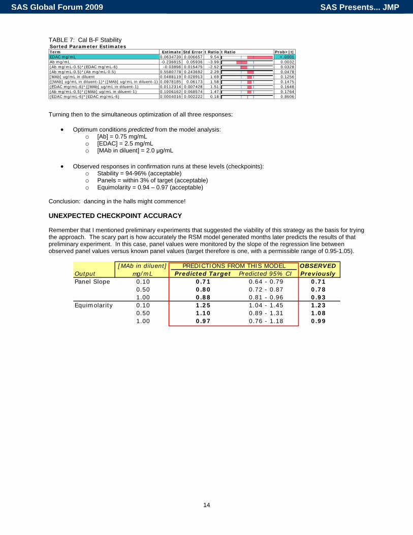
TABLE 7: Cal B-F Stability Sorted Parameter Estimates Term Estimate Std Error t Ratio t Ratio Prob>|t| EDAC mg/mL 0.0634739 0.006657 9.54 <.0001 Ab mg/mL -0.236815 0.05936 -3.99 0.0032 (Ab mg/mL-0.5)*(EDAC mg/mL-6) -0.03898 0.015475 -2.52 0.0328 (Ab mg/mL-0.5)*(Ab mg/mL-0.5) 0.5580778 0.243692 2.29 0.0478 [MAb] ug/mL in diluent 0.0488119 0.028913 1.69 0.1256 ([MAb] ug/mL in diluent-1)*([MAb] ug/mL in diluent-1) 0.0978185 0.06173 1.58 0.1475 (EDAC mg/mL-6)*([MAb] ug/mL in diluent-1) 0.0112314 0.007428 1.51 0.1648 (Ab mg/mL-0.5)*([MAb] ug/mL in diluent-1) 0.1006162 0.068574 1.47 0.1764 (EDAC mg/mL-6)*(EDAC mg/mL-6) 0.0004016 0.002222 0.18 0.8606 Turning then to the simultaneous optimization of all three responses:

• Optimum conditions predicted from the model analysis: o [Ab] = 0.75 mg/mL o [EDAC] = 2.5 mg/mL o [MAb in diluent] = 2.0 μg/mL

• Observed responses in confirmation runs at these levels (checkpoints):

o Stability = 94-96% (acceptable) o Panels = within 3% of target (acceptable) o Equimolarity = 0.94 – 0.97 (acceptable)

Conclusion: dancing in the halls might commence! UNEXPECTED CHECKPOINT ACCURACY Remember that I mentioned preliminary experiments that suggested the viability of this strategy as the basis for trying the approach. The scary part is how accurately the RSM model generated months later predicts the results of that preliminary experiment. In this case, panel values were monitored by the slope of the regression line between observed panel values versus known panel values (target therefore is one, with a permissible range of 0.95-1.05).

[MAb in diluent] OBSERVEDOutput mg/mL Predicted Target Predicted 95% CI PreviouslyPanel Slope 0.10 0.71 0.64 - 0.79 0.71

0.50 0.80 0.72 - 0.87 0.781.00 0.88 0.81 - 0.96 0.93

Equimolarity 0.10 1.25 1.04 - 1.45 1.230.50 1.10 0.89 - 1.31 1.081.00 0.97 0.76 - 1.18 0.99

PREDICTIONS FROM THIS MODEL

14


HANDY REFERENCES Anderson, Mark J. and Patrick J. Whitcomb. 2000. DOE Simplified – Practical Tools for Effective Experimentation. Portland, OR: Productivity, Inc. Anderson, Mark J. and Patrick J. Whitcomb. 2005. RSM Simplified – Optimizing Processes using Response Surface Methods for Design of Experiments. New York, NY: Productivity Press. Brandt, Doug and Steve Figard. 2005. Immunoassay Development in the In Vitro Diagnostics Industry. In: The Immunoassay Handbook, 3rd Ed. David Wild, editor. New York, NY: Elsevier, Inc. pages 136-143. ACKNOWLEDGMENTS I would like to acknowledge John Wass, statistician extraordinaire, former co-worker, and good friend, for motivation, helpful hints, and dutiful review of the content of this paper and subsequent presentation. CONTACT INFORMATION Steve Figard Abbott Laboratories Dept 09FE, Building AP20 100 Abbott Park Road Abbott Park, IL 60064-6015 (847) 937-9089 [email protected] SAS and all other SAS Institute Inc. product or service names are registered trademarks of SAS Institute Inc. in the USA and other countries. ® indicates USA registration. Other brand and product names are trademarks of their respective companies.

15


284-2009: The Basics of Experimental Design for...

Documents

Transcript of 284-2009: The Basics of Experimental Design for...