1 Automatic Calibration of MiCES Modules Craig Dowell University of Washington IRL Lab Seminar...
36
1 Automatic Calibration of MiCES Modules Craig Dowell University of Washington IRL Lab Seminar November 19, 2009
-
Upload
sharyl-porter -
Category
Documents
-
view
215 -
download
0
Transcript of 1 Automatic Calibration of MiCES Modules Craig Dowell University of Washington IRL Lab Seminar...

1
Automatic Calibration of MiCES Modules
Craig DowellUniversity of Washington
IRL Lab SeminarNovember 19, 2009

MiCES Automatic Calibration November 2009
2
Outline
• Quick Hardware Overview
• Graphical Analysis Tools
• Calibration Process
• Some Interesting Results
• Short Q & A

MiCES Automatic Calibration November 2009
3
MiCES Hardware Overview
• PET scanners have large numbers of detectors;
• Detectors arranged in concentric rings;
• Rings are composed of rows (of four PSPMTs each);
• Four (PS)PMTs per “cassette”;
• Cassette controlled by a “Rabbit Digital Board”;
• Two modules per digital board (master, slave);
• Two PMTs per module;
• From calibration perspective modules are independent;
• Calibration works per-module, or per-2-PMTs.

MiCES Automatic Calibration November 2009
4
MiCES Hardware Overview
• Fifteen settings (“knobs”) per module – Calibration means finding best settings for each of these knobs;
– For some definition of best.
Xx 2

MiCES Automatic Calibration November 2009
5
MiCES Hardware Overview
• High Voltage Setting– Affects both PMTs
– Used in calibration to position photopeak in histogram of PMT 0 (currently “best” means bin 155 – constant in cal code);
– Finest grained control (one bit = 5 bins).
• ASIC Gain (A, B, C & D) Setting– Allows for differences between PMTs
– Used in calibration to position photopeak in histogram of PMT 1 (currently “best” means bin 155);
– X+, X-, Y+, Y- are always set together;
– Not as fine grained (one bit = 15 bins).
MiCES Automatic Calibration November 2009
6
MiCES Hardware Overview
• CFD Threshold Setting– Used to adjust low energy side of histograms to common position “best” means bin
35;
– Cut out low energy noise but leave interesting signal.
• TDC Offset, TDC Gain Settings– Offset adjusts low side of TDC voltage divider network;
• “Best” means uniform distribution WRT lowest bins.
– Gain adjusts high side of TDC voltage divider network;• “Best” means uniform distribution WRT highest bins.
– Adjusts shape of TAC “ramp”;
– Offset too high means no low time-values;
– Gain too low means no high time-values.

MiCES Automatic Calibration November 2009
7
MiCES Hardware Overview
• Feedback for calibration is via histograms– Implemented in FPGA;
– Available to Rabbit processor;
– PMT divided into four quadrants;• Edge pixels not accumulated;
• Single histogram per quadrant;
• 256 energy bins per histogram.
– Timing information in fifth virtual “quadrant”;
• 32 bins of fine grained start time.

MiCES Automatic Calibration November 2009
8
Graphical Analysis Tools
• Written for the calibration project– C++;
– Really C;
– Some is similar code as in Rabbit calibration functions;
– Help make sense of odd histo data.
• Runs on Mac– Xcode + gnu toolchain + gnuplot
• Runs on Windows– Cygwin + gnu toolchain + gnuplot
• Freely available– Feel free to use any code you want

MiCES Automatic Calibration November 2009
9
Graphical Analysis Tools
• rabbit-histo-fit – Create energy histograms from module histogrammer raw data
and perform same fits as calibration code.

MiCES Automatic Calibration November 2009
10
Graphical Analysis Tools
• rabbit-tdc-plot – Create time histograms from module histogrammer raw data and
calculate same average and tolerance as calibration code.

MiCES Automatic Calibration November 2009
11
Graphical Analysis Tools
• crystal-map – Create surface plots of hit counts from MiCES map files;
– Not the same thing as an orgthog display, but similar.

MiCES Automatic Calibration November 2009
12
Graphical Analysis Tools
• map-read – Similar to rabbit-histo-plot but operates on MiCES map files;
– Used to check end-to-end results.

MiCES Automatic Calibration November 2009
13
Graphical Analysis Tools
• Orthog Display – Existing tool written in IDL;
– Combines position and energy information.

MiCES Automatic Calibration November 2009
14
Calibration
• First step is to adjust HV – Set default values for HV, ASIC 0 gain and take histo of PMT 0 and run fits to find
photopeak bin of each quadrant;
– Find average photopeak for PMT 0;
– Make small change in HV;
– Take histo of PMT 0 and run fits to find new photopeak bin of each quadrant;
– Find average photopeak for PMT 0;
– Assume responses to HV changes are linear, and calculate new HV to place average photopeak in desired bin (155);
– Set new HV and remember setting.
_ _
_ _ _
small change bits required change bits
measured after measured before bins desired measured before bins

MiCES Automatic Calibration November 2009
15
Calibration
• Second step is to adjust gain for PMT 1– Set default values for ASIC 1 gain;
– Take histo of PMT 1 and run fits to find photopeak bin of each quadrant;
– Find average photopeak for PMT 1;
– Make small change in ASIC 1 gain;
– Take histo of PMT 1 and run fits to find new photopeak bin of each quadrant;
– Find average photopeak for PMT 1;
– Assume responses to gain changes are linear, and calculate new gain to place average photopeak in desired bin (155);
– Set new ASIC 1 gain and remember setting.

MiCES Automatic Calibration November 2009
16
Calibration
• Third, fourth steps are to set CFD threshold for PMT 0 and 1– Set CFD threshold to max;
– Take histo of PMT and find low energy edge of backscatter peak in each quadrant – calculate average over quadrants
– Make small downward change in CFD threshold;
– Take histo of PMT and find low energy edge of backscatter peak in each quadrant – calculate average over quadrants;
– Assume responses to CFD threshold are linear, and calculate new gain to place average edge in desired bin (35);
– Set new CFD threshold and remember setting;
– Repeat for second PMT.

MiCES Automatic Calibration November 2009
17
Calibration
• Fifth, sixth steps are to set TDC offset and gain for PMT 0 and 1– Set TDC offset and gain to default
– Take histo of PMT and find average counts in center bins;
– If lowest bin not in range, binary search (change setting, take histo) for TDC offset that puts lowest bin closest to average;
– Take histo of PMT and find average counts in center bins;
– If highest bin not in range, binary search (change setting, take histo) for TDC gain that puts highest bin closest to average;
– Set new TDC offset and gain and remember settings;
– Repeat for second PMT.

MiCES Automatic Calibration November 2009
18
Calibration
• Final step is to write settings to flash– HV DAC setting;
– ASIC 0 gain (individual channels A, B, C, D);
– ASIC 0 CFD Threshold;
– ASIC 0 TDC offset;
– ASIC 0 TDC gain;
– ASIC 1 gain (individual channels A, B, C, D);
– ASIC 1 CFD Threshold;
– ASIC 1 TDC offset;
– ASIC 1 TDC gain.
• Total of fifteen knobs adjusted
• Values can be restored from flash at power-on

MiCES Automatic Calibration November 2009
19
Calibration
• Before and after energy histograms

MiCES Automatic Calibration November 2009
20
Calibration
• Before and after time histograms

MiCES Automatic Calibration November 2009
21
Interesting Results 1
• Already seen one– Funny shaped photopeak;
– Backscatter peak larger than photopeak.

MiCES Automatic Calibration November 2009
22
Interesting Results 1
• Why?– Each PSPMT is really an array of miniature PMTs;
– Gain of each miniature PMT can vary by more than 30% (source Hamamatsu).

MiCES Automatic Calibration November 2009
23
Interesting Results 1
• Why?– Rabbit histograms give finer granularity;
– Another case: three different photopeaks?

MiCES Automatic Calibration November 2009
24
Interesting Results 1
• Why?– Orthog display shows
phenomenon clearly;
– Notice gain drop overabout one sixth of PMTwidth in saggital slice;
– Six X-direction anodesper PMT.

MiCES Automatic Calibration November 2009
25
Interesting Results 1
• This means different PMT quadrants exhibit very different photopeaks.– Quadrant 1

MiCES Automatic Calibration November 2009
26
Interesting Results 1
• This means different PMT quadrants exhibit very different photopeaks– Quadrant 2

MiCES Automatic Calibration November 2009
27
Interesting Results 1
• This means different PMT quadrants exhibit very different photopeaks– Quadrant 3
MiCES Automatic Calibration November 2009
28
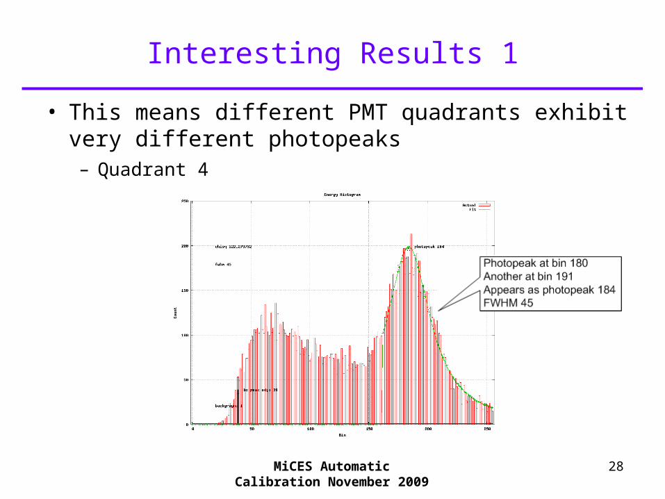
Interesting Results 1
• This means different PMT quadrants exhibit very different photopeaks– Quadrant 4

MiCES Automatic Calibration November 2009
29
Interesting Results 1
• Implications– Can’t just look for highest count and assume that is photopeak –
it might be a backscatter peak;
– Differences between quadrants within one PMT are often greater than between different PMTs;
– If looking for unscattered annihilation photons by filtering on 511 KeV photons, you want to look for hits around the photopeak – but positions of photopeaks have 30% tolerance;
• Can do calibration on end-to-end system using map files to come up with compensation values since map files have pixel resolution;
• Not possible with current FPGA histogrammer.
– It’s hard to tell where the cut value is between a good module/PMT and a bad one.

MiCES Automatic Calibration November 2009
30
Interesting Results 2
• Delamination of Crystals– It is suspected that high temperatures in the lab caused
delamination of crystals;
– crystal-map tool shows reduced hit counts quite clearly.
MiCES Automatic Calibration November 2009
31
Interesting Results 3
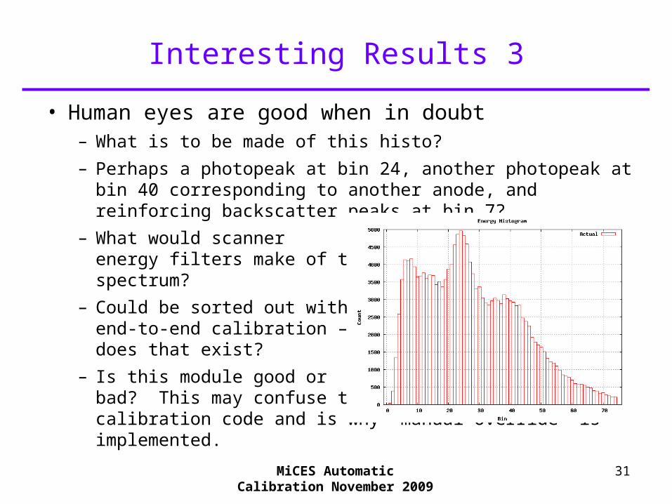
• Human eyes are good when in doubt– What is to be made of this histo?
– Perhaps a photopeak at bin 24, another photopeak at bin 40 corresponding to another anode, and reinforcing backscatter peaks at bin 7?
– What would scanner energy filters make of this spectrum?
– Could be sorted out withend-to-end calibration –does that exist?
– Is this module good orbad? This may confuse thecalibration code and is why “manual override” is implemented.

MiCES Automatic Calibration November 2009
32
Interesting Results 3
• Human eyes are good when in doubt– What is to be made of this histo?
– Hardware problem?
– No Lorentzian-likephotopeak, so chi-squarewill be huge.
– I provide a “test” functionwith some initial cut values on parameterslike chi-square of fit.
– Needs furtherdevelopment.
– Right now, main calibration routines will just print large chi-square statistics and will continue as much as possible.

MiCES Automatic Calibration November 2009
33
Interesting Results n
• There are many “novel” histograms laying around in the system;
• When I started this project, I went through many of them to try and get my bearings and was often completely baffled;
• I think many of the odd histograms were due to various failures in the system. Dan tells me that cables are notoriously fickle;
• I tried to make the calibration code fairly robust, but I am (and my code is) still surprised by what sometimes happens.

MiCES Automatic Calibration November 2009
34
Resources
• I have passed around an “Orange Book” that describes all of this in excruciating detail;
• It shows where all of the analysis code lives, on Windows and Mac, and how to build it;
• Shows how to run and interpret all of the outputs of the various pieces of code;
• Includes a CD-ROM with all of the code, manual and this presentation on it;
• This is all freely usable in the sense of GPL. If you think any of my bits may be useful, feel free to use them in any way you want.

MiCES Automatic Calibration November 2009
35
Lessons Learned
• The hardest part was understanding why so many histograms were so “oddly” shaped;
• Spend time up front writing tools and scripts for gathering, reducing and presenting data – it is well worth it;
• Looking at lots of histograms with human eyes is important – run code on as many different modules as possible, as soon as possible;
• Don’t be afraid to throw things away if they aren’t working out;
• It’s a research device, expect it to be broken sometimes.

MiCES Automatic Calibration November 2009
36
Automatic Calibration of MiCES Modules
Short Q and A

![Index []...2003/01/28 · IRL Jack O'Leary 04/11/1997 IRL Peter Lynch 26/11/1997 IRL Darragh McElhinney 2000 IRL Fearghal Curtin 14/07/1998 IRL Charlie O'Donovan 06/08/1999 IRL Barry](https://static.fdocuments.us/doc/165x107/5e9ad3bf924b7b6d1915a79a/index-20030128-irl-jack-oleary-04111997-irl-peter-lynch-26111997.jpg)