
Well-to-wheels Analysis of Future Automotive Fuels and...
108
EUR 24952 EN - 2011 Well-to-wheels Analysis of Future Automotive Fuels and Powertrains in the European Context WTT APPENDIX 1 Description of individual processes and detailed input data R. Edwards European Commission Joint Research Centre, Institute for Energy J-F. Larivé CONCAWE J-C. Beziat Renault/EUCAR
Transcript of Well-to-wheels Analysis of Future Automotive Fuels and...

EUR 24952 EN - 2011
Well-to-wheels Analysis of Future Automotive Fuels and Powertrains
in the European Context WTT APPENDIX 1
Description of individual processes and detailed input data
R. EdwardsEuropean Commission Joint Research Centre, Institute for Energy
J-F. LarivéCONCAWE
J-C. BeziatRenault/EUCAR

The mission of the JRC-IE is to provide support to Community policies related to both nuclear and non-nuclear energy in order to ensure sustainable, secure and efficient energy production, distribution and use. European Commission Joint Research Centre Institute for Energy and Transport Contact information Address: Ispra Site I – 21027 (Va) E-mail: [email protected] Tel.: +39 0332 783902 Fax: +39 0332 785236 http://iet.jrc.ec.europa.eu/about-jec http://www.jrc.ec.europa.eu/ Legal Notice Neither the European Commission nor any person acting on behalf of the Commission is responsible for the use which might be made of this publication.
Europe Direct is a service to help you find answers to your questions about the European Union
Freephone number (*):
00 800 6 7 8 9 10 11
(*) Certain mobile telephone operators do not allow access to 00 800 numbers or these calls may be billed.
A great deal of additional information on the European Union is available on the Internet. It can be accessed through the Europa server http://europa.eu/ JRC 65998 EUR 24952 EN ISBN 978-9279-21395-3 ISSN 1831-9424 doi:10.2788/79018 Luxembourg: Publications Office of the European Union © European Union, 2011 Reproduction is authorised provided the source is acknowledged Printed in Italy

WELL-TO-WHEELS ANALYSIS OF FUTURE AUTOMOTIVE FUELS AND POWERTRAINS
IN THE EUROPEAN CONTEXT
WELL-to-TANK Report - Appendix 1
Version 3c, July 2011
http://iet.jrc.ec.europa.eu/about-jec [email protected]

WTT Report v3c July 2011 – Appendix 1 Page 4 of 108
This report is available as an ADOBE pdf file on the JRC/IES website at:
http://iet.jrc.ec.europa.eu/about-jec Questions and remarks may be sent to:
[email protected] Notes on version number: This document reports on the third release of this study replacing data made available since November 2008. The original version 1b was published in December 2003.
WTT Report v3c July 2011 – Appendix 1 Page 5 of 108
Description of individual processes and detailed input data All WTT data is stored in LBST's E3 database and that software was used to calculate the energy and GHG balances of the pathways. This appendix provides full detail of the input data. It consists in two elements: • A series of tables giving input data to each process, • A textual description and justification of each process. The information has been split into logical sections each incorporating the processes involved in a number of related pathways. The process that are new to this version 3 or have been updated, as compared to version 2c are highlighted in yellow. In this appendix both energy and GHG figures are shown per unit energy content of the output of the particular process (MJ), i.e. NOT of the output of the total pathway (e.g. the energy required for wheat farming is shown per MJ of wheat grain, rather than MJ of ethanol). This has to be kept in mind when comparing figures in the appendix with those in WTT Appendix 2 where figures pertaining to each step of a pathway are expressed per MJ of the final fuel. The energy figures are expressed as net total energy expended (MJxt) in each process (i.e. excluding the energy transferred to the final fuel) per unit energy content of the output of the process (MJ). Where fuels or intermediate energy sources (e.g. electricity) are used in a process the total primary energy (MJp) is allocated to the process including the energy necessary to make the fuel or the electricity. Example: • If a process requires 0.1 MJ of electricity per MJ output, the expended energy is expressed as 0.1 MJx/MJ. • If electricity is generated with a 33% efficiency, the primary energy associated to 1 MJ of electricity is 3 MJp. • The total primary energy associated to the process is then 3 x 0.1 = 0.3 MJp/MJ. All energy is accounted for regardless of the primary energy source, i.e. including renewable energy. This is necessary to estimate the energy footprint of each process and each pathway. The share of fossil energy in each complete pathway is shown in the overall pathway energy balance (see WTT Appendix 2). The CO2 figures represent the actual emissions occurring during each process. When CO2 emissions stem from biomass sources only the net emissions are counted i.e. excluding CO2 emitted when burning the biomass. The figures used in this study and described in this appendix are generally based on literature references as given. In a number of cases, particularly with regards to oil-based pathways, we have used figures considered as typical in the industry and generally representing the combined views of a number of experts. Where no specific reference is given, the figures are the result of standard physical calculations based on typical parameters. This is the case for instance for CNG or hydrogen compression energy.

WTT Report v3c July 2011 – Appendix 1 Page 6 of 108
Most processes include a line labelled "Primary energy consumption and emissions": this is an approximate and simplified calculation intended for the reader's guidance. The full calculation has been carried out by LBST's E3 database resulting in the figures in WTT Appendix 2. Where appropriate we have specified a range of variability associated with a probability distribution either normal (Gaussian), double-triangle for asymmetrical distribution or equal (all values in the range equally probable). The equal distribution has been used when representing situations where a range of technologies or local circumstances may apply, all being equally plausible. For the complete pathway, a variability range is estimated by combining the individual ranges and probability distributions with the Monte-Carlo method.
WTT Report v3c July 2011 – Appendix 1 Page 7 of 108
Table of contents
1 Useful conversion factors and calculation methods 13
1.1 General 13 1.2 Factors for individual fuels 13 1.3 GHG calculations 15
2 Fuels properties 16
2.1 Standard properties of fuels 16 2.2 Detailed composition of natural gas per source 17 2.3 Deemed composition of LPG 18
3 Common processes 19 Z1 Diesel production 19 Z2 Road tanker 19 Z3 Heavy Fuel Oil (HFO) production 20 Z4 Product carrier (50 kt) 20 Z5 Rail transport 20 Z6 Marginal use of natural gas 20 Z7 Electricity (EU-mix) 20
4 Crude oil – based fuels provision 21 4.1 Crude oil, diesel fuel 21
CO1 Crude oil production 22 CO2 Crude oil transportation 22 CD1 Crude oil refining, marginal diesel 23 CD2 Diesel transport 23 CD3 Diesel depot 23 CD4 Diesel distribution 23
4.2 Gasoline 24 CG1/4 Gasoline 24
4.3 Naphtha 25 CN1/4 Naphtha 25
5 Natural gas (NG) provision (including CNG) 26

WTT Report v3c July 2011 – Appendix 1 Page 8 of 108
5.1 Natural gas extraction and processing 26 GG1 NG extraction & processing 26 GG2 On-site electricity generation 27 GG2C On-site electricity generation with CCS (CO2 capture and storage) 27
5.2 Long distance pipeline transport 27 5.3 LNG 29
GR1 NG liquefaction 30 GR1C Liquefaction with CO2 capture 30 GR2 LNG loading terminal 30 GR3 LNG transport 30 GR4 LNG unloading terminal 30 GR5 LNG vaporisation 31 GR6 LNG distribution (road tanker) 31 GR7 LNG to CNG (vaporisation/compression) 31
5.4 Natural gas distribution, CNG dispensing 31 GG3 NG trunk distribution 32 GG4 NG local distribution 32 GG5 CNG dispensing (compression) 32 Note on CO2 emissions from natural gas combustion: 33
6 Synthetic fuels and hydrogen production from NG 34
6.1 Syn-diesel, Methanol, DME 34 GD1 NG to syn-diesel plant (GTL) 35 GD1C NG to syn-diesel plant with CO2 capture 35 GA1 NG to methanol plant 35 GT1 NG to DME plant 36 GT1C NG to DME plant with CO2 capture 36
6.2 Natural gas to hydrogen 36 GH1a NG to hydrogen (steam reforming, on-site, 2 MW hydrogen,) 36 GH1b NG to hydrogen (steam reforming, central plant, 100-300 MW hydrogen) 36 GH1bC NG to hydrogen (steam reforming, central plant, 100-300 MW hydrogen) with CO2 capture 37
7 LPG and ethers 38 LR1 LPG production 38 BU1 n-butane to isobutene 38 EH1 ETBE manufacture (large plant) 38 MH1 MTBE manufacture (large plant) 39
8 Synthetic fuels and hydrogen production from coal 40 KB1 Lignite/brown coal provision 41
WTT Report v3c July 2011 – Appendix 1 Page 9 of 108
KO1 Hard coal provision (EU-mix) 41 KH1 Coal to hydrogen 41 KH1C Coal to hydrogen with CO2 capture 41 KA1/E1 Coal to methanol or DME 41 KD1 Coal to synthetic diesel 41 KD1C Coal to synthetic diesel with CO2 capture 41
9 Farming processes 42 SB1 Sugar Beet Farming 44 WT1a-c Wheat Farming 44 SC1 Sugar cane farming (Brazil) 44 WF1 Wood Farming 45 RF1 Rapeseed Farming 47 SF1 Sunflower Seed Farming 47 SY1 Soy Bean Farming 48 PO1 Palm Oil Plantation 49 CR1 Corn farming 49
10 Production of agro-chemicals 51 AC1-3 N/P/K Fertilizer Provision 52 AC4 Lime (CaO+CaCO3) Provision 52 AC5 Provision of other farming inputs 52
11 Biomass transport 53 Z8a 40 tonne truck for dry products 54 Z8b 12 tonne truck for dry products 54 Z10 Ocean-going bulk carrier 54 SY2 Soy bean transport 55 PO2 Palm FFB 55 PO4a Palm oil road transport 56 PO4b Vegetable oil shipping 56
12 Biogas from organic materials 57
12.1 Biogas from organic waste 57 Heat and power generation in the biogas plant 58 BG2 Waste biomass to upgraded biogas 59 BG3 Waste biomass to electricity (small scale) 60
12.2 Biogas from crops 60 WB1 Whole wheat to biogas 61 WB2 Double cropping whole plant maize and barley to biogas 61
13 Conversion processes for “conventional biofuels” 62

WTT Report v3c July 2011 – Appendix 1 Page 10 of 108
13.1 Credit Calculation for Animal Feed By-Products 62 13.2 Ethanol from sugar beet 63
SB3a Ethanol from sugar beet, pulp used as animal feed, slops not used 63 SB3b Sugar beet to ethanol, pulp to animal feed, slops to biogas 64 SB3c Ethanol from sugar beet, pulp burned to produce heat and electricity, slops to biogas 64
13.3 Ethanol from wheat grain 65 WT3 Wheat Grain Handling 66 WT4a Conventional natural gas boiler 66 WT4b Combined cycle gas turbine 66 WT4c Lignite boiler CHP 66 WT4d Straw boiler CHP 66 WTDa Credits for DDGS as animal feed 67 WTDb Credits for DDGS as fuel 67 WT4e Wheat grain to ethanol, DDGS to biogas 67
13.4 Ethanol from sugar cane (Brazil) 68 SC3a Sugar cane ethanol with credit for surplus bagasse 68 SC3b Sugar cane ethanol, no credit for surplus bagasse 68
13.5 Biodiesel for plant oil 69 RO3a/b Rapeseed Oil Extraction 70 SO3a/b Sunflower Oil Extraction 70 SY3a/b Soy beans to raw oil: extraction 71 PO3 Palm FFB to raw oil: extraction 72 PO3a Palm Oil - Methane emissions from waste 72 PO3b Palm Oil - Credit for surplus heat (diesel) 73 RO4 Plant Oil Refining 73 RO/SO5 Esterification (methanol) 75 RO/SO6 Esterification (ethanol) 75
13.6 Processes to make materials needed for biomass processing and credit calculations 76 C6 Pure CaO for Processes 77 C7 Sulphuric Acid 77 C8 Ammonia 77 C10 Propylene Glycol 77 SY3 Soy meal from crushing soy beans 77 SYML Complete soy bean meal production chain 78
13.7 Hydrotreated Plant Oil 78 OY1a Plant Oil Hydrotreating (NexBTL) 79 OY1b Plant Oil Hydrotreating (UOP) 79
14 Synthetic fuels and hydrogen production from farmed wood and wood waste 80 WW1 Forest residuals chipping 80

WTT Report v3c July 2011 – Appendix 1 Page 11 of 108
14.1 Wood gasification to hydrogen 81 W3d Large scale (200 MW) 81 W3e Small scale (10MW) 81
14.2 Synthetic fuels from wood gasification 82 W3f Synthetic Diesel from Wood 82 W3g Wood to methanol or DME 82
14.3 Ethanol from cellulosic biomass (farmed wood, wood waste and straw) 84 W3j Ethanol from woody biomass; worst/best case 85 W3k Ethanol from straw 85
14.4 Synthetic fuels and hydrogen from waste wood via Black Liquor 86 BLD/M Wood waste to DME/Methanol 86 BLS Wood waste to FT via black liquor gasification 88 BLH Wood waste to hydrogen via black liquor gasification 89
15 Heat and Electricity (co)Generation 91
15.1 Electricity only 91 GE Electricity from NG 92 KE1 Electricity from coal (conv. boiler) 92 KE2 Electricity from coal (IGCC) 92 W3a Electricity from wood steam boiler 92 W3b Electricity from 200 MWth wood gasifier 92 W3c Electricity from 10 MWth wood gasifier 92 BLE Electricity from waste wood via black liquor 93 W3h Wood co-firing in coal-fired power station 93 DE Electricity from wind 93 NE1 Nuclear fuel provision 93 NE2 Electricity from nuclear 93
15.2 Heat only 94 15.3 Combined Heat and Power (CHP) 95
16 Hydrogen from electrolysis 96 YH Hydrogen from electrolysis 96
17 Hydrogen distribution and dispensing (all sources) 97 CH1a/b Gaseous hydrogen distribution 98 CH2 Liquid hydrogen vaporisation/compression 98 CH3 Gaseous hydrogen compression 98 LH1 Hydrogen liquefaction 98 LH2 Liquid hydrogen long-distance transport 98 LH3 Liquid hydrogen distribution 99

WTT Report v3c July 2011 – Appendix 1 Page 12 of 108
18 Synthetic fuels distribution and dispensing (all sources) 100 DS1 Synthetic diesel loading and handling (remote) 100 DS2 Synthetic diesel sea transport 100 DS3 Synthetic diesel depot 100 DS4 Synthetic diesel distribution (blending component) 101 DS5a/b Synthetic diesel distribution (neat) 101 ME1 Methanol handling and loading (remote) 102 ME2 Methanol sea transport 103 ME3 Methanol depot 103 ME4a/b Methanol distribution and dispensing 103 DE1-4 DME distribution and dispensing 103
19 Bio-fuels distribution 104
20 References 105

WTT Report v3c July 2011 – Appendix 1 Page 13 of 108
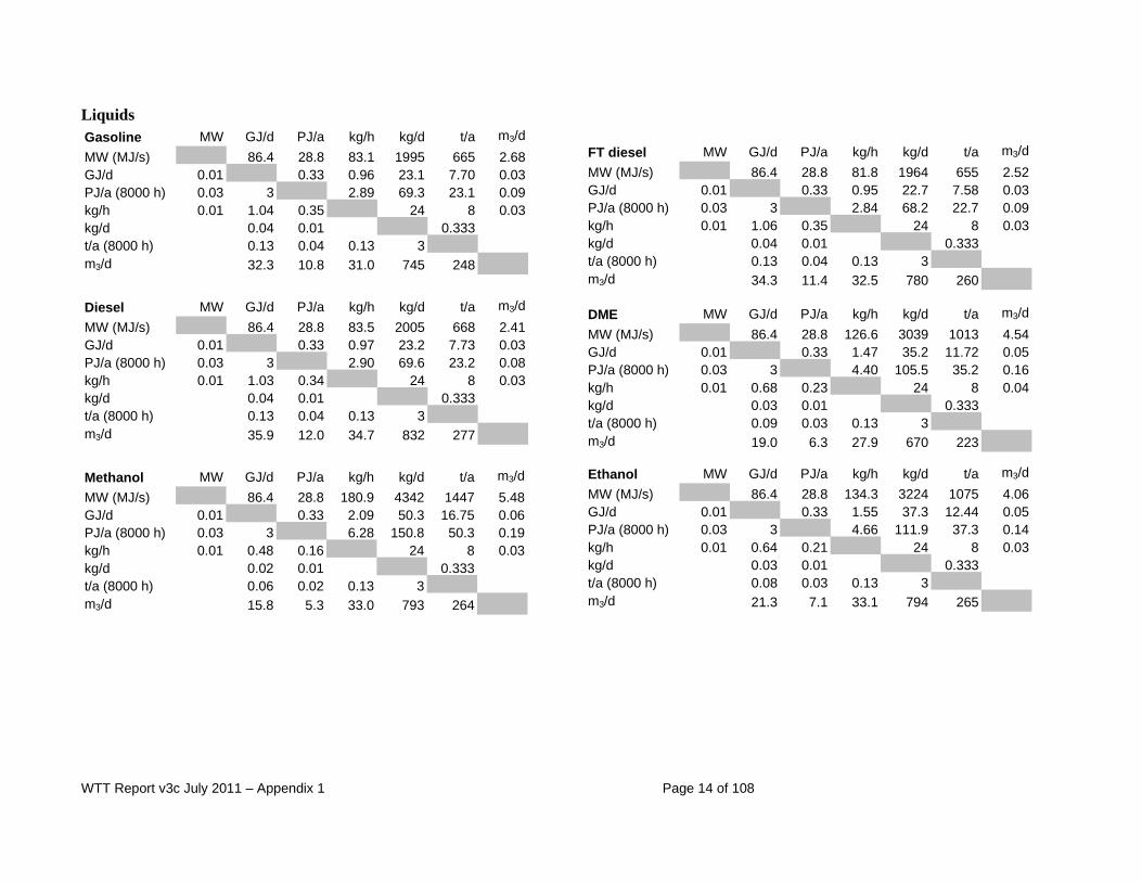
1 Useful conversion factors and calculation methods 1.1 General 1 kWh = 3.6 MJ = 3412 Btu 1 Mtoe = 42.6 PJ 1 MW = 1 MJ/s = 28.8 PJ/a (8000 h) 1 t crude oil ~ 7.4 bbl 1 Nm3 of EU-mix NG ~ 0.8 kg ~ 40 MJ (i.e. 1 Nm3 of NG has approximately the same energy content as 1 kg of crude oil) 1.2 Factors for individual fuels Gases
NG EU-mix MW GJ/d PJ/a kg/h kg/d t/a Nm3/hMW (MJ/s) 86.4 28.8 80.4 1929 643 102GJ/d 0.012 0.333 0.930 22.3 7.4 1.18PJ/a (8000 h) 0.035 3 2.79 67.0 22.3 3.53kg/h 0.012 1.07 0.36 24 8 1.27kg/d 0.04 0.01 0.33 0.05t/a (8000 h) 0.13 0.04 0.13 3 0.16Nm3/h 0.85 0.28 0.79 19.0 6.3
Hydrogen MW GJ/d PJ/a kg/h kg/d t/a Nm3/hMW (MJ/s) 86.4 28.8 30.0 719 240 336GJ/d 0.012 0.333 0.347 8.3 2.8 3.89PJ/a (8000 h) 0.035 3 1.04 25.0 8.3 11.66kg/h 0.033 2.88 0.96 24 8 11.20kg/d 0.12 0.04 0.33 0.47t/a (8000 h) 0.36 0.12 0.13 3 1.40Nm3/h 0.26 0.09 0.09 2.1 0.7
Methane MW GJ/d PJ/a kg/h kg/d t/a Nm3/hMW (MJ/s) 86.4 28.8 72.0 1728 576 101GJ/d 0.012 0.333 0.833 20.0 6.7 1.17PJ/a (8000 h) 0.035 3 2.50 60.0 20.0 3.50kg/h 0.014 1.20 0.40 24 8 1.40kg/d 0.05 0.02 0.33 0.06t/a (8000 h) 0.15 0.05 0.13 3 0.18Nm3/h 0.86 0.29 0.71 17.1 5.7
WTT Report v3c July 2011 – Appendix 1 Page 14 of 108
Liquids Gasoline MW GJ/d PJ/a kg/h kg/d t/a m3/dMW (MJ/s) 86.4 28.8 83.1 1995 665 2.68GJ/d 0.01 0.33 0.96 23.1 7.70 0.03PJ/a (8000 h) 0.03 3 2.89 69.3 23.1 0.09kg/h 0.01 1.04 0.35 24 8 0.03kg/d 0.04 0.01 0.333t/a (8000 h) 0.13 0.04 0.13 3m3/d 32.3 10.8 31.0 745 248 Diesel MW GJ/d PJ/a kg/h kg/d t/a m3/dMW (MJ/s) 86.4 28.8 83.5 2005 668 2.41GJ/d 0.01 0.33 0.97 23.2 7.73 0.03PJ/a (8000 h) 0.03 3 2.90 69.6 23.2 0.08kg/h 0.01 1.03 0.34 24 8 0.03kg/d 0.04 0.01 0.333t/a (8000 h) 0.13 0.04 0.13 3m3/d 35.9 12.0 34.7 832 277 Methanol MW GJ/d PJ/a kg/h kg/d t/a m3/dMW (MJ/s) 86.4 28.8 180.9 4342 1447 5.48GJ/d 0.01 0.33 2.09 50.3 16.75 0.06PJ/a (8000 h) 0.03 3 6.28 150.8 50.3 0.19kg/h 0.01 0.48 0.16 24 8 0.03kg/d 0.02 0.01 0.333t/a (8000 h) 0.06 0.02 0.13 3m3/d 15.8 5.3 33.0 793 264
FT diesel MW GJ/d PJ/a kg/h kg/d t/a m3/dMW (MJ/s) 86.4 28.8 81.8 1964 655 2.52GJ/d 0.01 0.33 0.95 22.7 7.58 0.03PJ/a (8000 h) 0.03 3 2.84 68.2 22.7 0.09kg/h 0.01 1.06 0.35 24 8 0.03kg/d 0.04 0.01 0.333t/a (8000 h) 0.13 0.04 0.13 3m3/d 34.3 11.4 32.5 780 260
DME MW GJ/d PJ/a kg/h kg/d t/a m3/dMW (MJ/s) 86.4 28.8 126.6 3039 1013 4.54GJ/d 0.01 0.33 1.47 35.2 11.72 0.05PJ/a (8000 h) 0.03 3 4.40 105.5 35.2 0.16kg/h 0.01 0.68 0.23 24 8 0.04kg/d 0.03 0.01 0.333t/a (8000 h) 0.09 0.03 0.13 3m3/d 19.0 6.3 27.9 670 223
Ethanol MW GJ/d PJ/a kg/h kg/d t/a m3/dMW (MJ/s) 86.4 28.8 134.3 3224 1075 4.06GJ/d 0.01 0.33 1.55 37.3 12.44 0.05PJ/a (8000 h) 0.03 3 4.66 111.9 37.3 0.14kg/h 0.01 0.64 0.21 24 8 0.03kg/d 0.03 0.01 0.333t/a (8000 h) 0.08 0.03 0.13 3m3/d 21.3 7.1 33.1 794 265
WTT Report v3c July 2011 – Appendix 1 Page 15 of 108
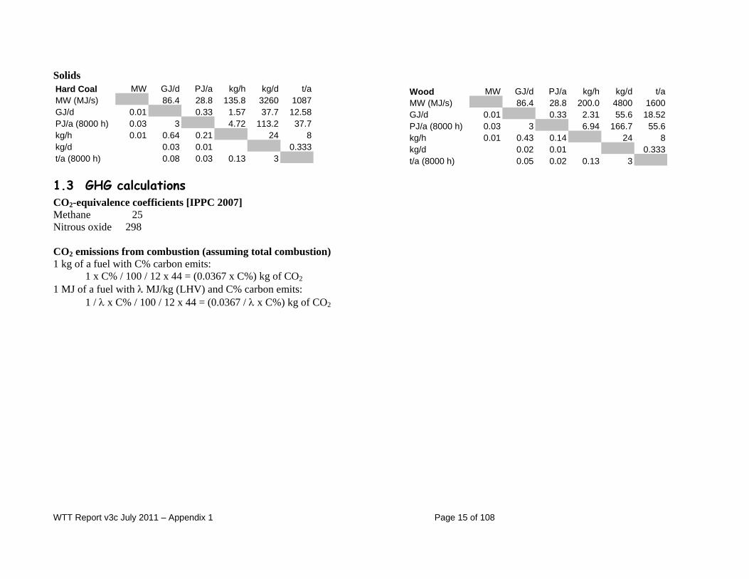
Solids Hard Coal MW GJ/d PJ/a kg/h kg/d t/aMW (MJ/s) 86.4 28.8 135.8 3260 1087GJ/d 0.01 0.33 1.57 37.7 12.58PJ/a (8000 h) 0.03 3 4.72 113.2 37.7kg/h 0.01 0.64 0.21 24 8kg/d 0.03 0.01 0.333t/a (8000 h) 0.08 0.03 0.13 3 1.3 GHG calculations CO2-equivalence coefficients [IPPC 2007] Methane 25 Nitrous oxide 298 CO2 emissions from combustion (assuming total combustion) 1 kg of a fuel with C% carbon emits:
1 x C% / 100 / 12 x 44 = (0.0367 x C%) kg of CO2 1 MJ of a fuel with λ MJ/kg (LHV) and C% carbon emits: 1 / λ x C% / 100 / 12 x 44 = (0.0367 / λ x C%) kg of CO2
Wood MW GJ/d PJ/a kg/h kg/d t/aMW (MJ/s) 86.4 28.8 200.0 4800 1600GJ/d 0.01 0.33 2.31 55.6 18.52PJ/a (8000 h) 0.03 3 6.94 166.7 55.6kg/h 0.01 0.43 0.14 24 8kg/d 0.02 0.01 0.333t/a (8000 h) 0.05 0.02 0.13 3
WTT Report v3c July 2011 – Appendix 1 Page 16 of 108
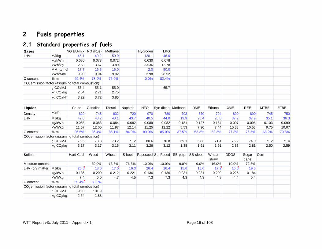
2 Fuels properties 2.1 Standard properties of fuels Gases NG EU-mix NG (Rus) Methane Hydrogen LPGLHV MJ/kg 45.1 49.2 50.0 120.1 46.0
kg/kWh 0.080 0.073 0.072 0.030 0.078kWh/kg 12.53 13.67 13.89 33.36 12.78MM, g/mol 17.7 16.3 16.0 2.0 50.0kWh/Nm3 9.90 9.94 9.92 2.98 28.52
C content % m 69.4% 73.9% 75.0% 0.0% 82.4%CO2 emission factor (assuming total combustion)
g CO2/MJ 56.4 55.1 55.0 65.7kg CO2/kg 2.54 2.71 2.75kg CO2/Nm 3.22 3.72 3.85
Liquids Crude Gasoline Diesel Naphtha HFO Syn diesel Methanol DME Ethanol XME REE MTBE ETBE
Density kg/m3 820 745 832 720 970 780 793 670 794 890 890 745 750LHV MJ/kg 42.0 43.2 43.1 43.7 40.5 44.0 19.9 28.4 26.8 37.2 37.9 35.1 36.3
kg/kWh 0.086 0.083 0.084 0.082 0.089 0.082 0.181 0.127 0.134 0.097 0.095 0.103 0.099kWh/kg 11.67 12.00 11.97 12.14 11.25 12.22 5.53 7.90 7.44 10.33 10.53 9.75 10.07
C content % m 86.5% 86.4% 86.1% 84.9% 89.0% 85.0% 37.5% 52.2% 52.2% 77.3% 76.5% 68.2% 70.6%CO2 emission factor (assuming total combustion)
g CO2/MJ 75.5 73.3 73.2 71.2 80.6 70.8 69.1 67.3 71.4 76.2 74.0 71.2 71.4kg CO2/kg 3.17 3.17 3.16 3.11 3.26 3.12 1.38 1.91 1.91 2.83 2.81 2.50 2.59
Solids Hard Coal Wood Wheat S beet Rapeseed SunFseed SB pulp SB slops Wheat straw
DDGS Sugar cane
Corn
Moisture content 30.0% 13.5% 76.5% 10.0% 10.0% 9.0% 9.0% 16.0% 10.0% 72.5%LHV (dry matter) MJ/kg 26.5 18.0 17.0 16.3 26.4 26.4 15.6 15.6 17.2 16.0 19.6
kg/kWh 0.136 0.200 0.212 0.221 0.136 0.136 0.231 0.231 0.209 0.225 0.184kWh/kg 7.4 5.0 4.7 4.5 7.3 7.3 4.3 4.3 4.8 4.4 5.4
C content % m 69.4% 50.0%CO2 emission factor (assuming total combustion)
g CO2/MJ 96.0 101.9kg CO2/kg 2.54 1.83

WTT Report v3c July 2011 – Appendix 1 Page 17 of 108
2.2 Detailed composition of natural gas per source Origin CIS NL UK Norway Algeria EU-mix
%mol %mShare in EU-mix 21.4% 22.0% 30.4% 11.8% 14.4%H2 0.0% 0.0% 0.5% 0.5% 0.8% 0.3% 0.0%C1 98.4% 81.5% 86.0% 86.0% 92.1% 88.5% 79.9%C2 0.4% 2.8% 8.8% 8.8% 1.0% 4.6% 7.7%C3 0.2% 0.4% 2.3% 2.3% 0.0% 1.1% 2.7%C4 0.1% 0.1% 0.1% 0.1% 0.0% 0.1% 0.3%C5 0.0% 0.0% 0.0% 0.0% 0.0% 0.0% 0.0%C6 0.0% 0.0% 0.0% 0.0% 0.0% 0.0% 0.0%C7 0.0% 0.0% 0.0% 0.0% 0.0% 0.0% 0.0%CO2 0.1% 1.0% 1.5% 1.5% 0.0% 0.9% 2.2%N2 0.8% 14.2% 0.8% 0.8% 6.1% 4.5% 7.1%
100.0% 100.0% 100.0% 100.0% 100.0% 100.0% 100.0%MM (g/mol) 16.3 18.5 18.4 18.4 16.8 17.7Density (kg/Nm3) 0.727 0.827 0.820 0.820 0.750 0.791LHV (MJ/Nm3) 35.7 31.4 38.6 38.6 33.7 35.7LHV (GJ/t) 49.2 38.0 47.1 47.1 44.9 45.1MON (CARB) 138.2 132.9 122.3 122.3 138.0 129.2Methane number (CARB) 105.3 96.8 79.6 79.6 105.0 90.7Methane number (DK) 96.6 93.3 75.7 75.7 98.3 84.1 Source: GEMIS MON and Methane number methods references: 'Algorithm for methane number determination for natural gasses' (sic) by Paw Andersen, Danish Gas Technology Centre, Report R9907, June 1999 http://uk.dgc.dk/publications/algotitme.htm CARB: http://www.arb.ca.gov/regact/cng-lpg/cng-lpg.htm The EU-mix is the gas that is deemed to be available to the vehicle as CNG.

WTT Report v3c July 2011 – Appendix 1 Page 18 of 108
2.3 Deemed composition of LPG Component % m/m % v/v MM LHV (GJ/t) C (%m/m) H (%m/m)C1 0.1 0.3 16 50.1 75.0 25.0C2 2.4 4.0 30 47.5 80.0 20.0C2= 0.5 0.9 28 47.2 85.7 14.3C3 40.0 45.4 44 46.4 81.8 18.2C3= 1.0 1.2 42 45.8 85.7 14.3nC4 30.0 25.8 58 45.8 82.8 17.2iC4 22.0 19.0 58 45.7 82.8 17.2C4= 1.5 1.3 56 45.3 85.7 14.3iC4= 1.5 1.3 56 45.1 85.7 14.3nC5 1.0 0.7 72 45.4 83.3 16.7Total 100.0 100.0 50 46.0 82.4 17.6TotalC2- 3.0C3 41.0C4 55.0 CO2 emission factorC5+ 1.0 3.02 t CO2 / tOlefins 4.5 65.7 kg CO2 / GJ

WTT Report v3c July 2011 – Appendix 1 Page 19 of 108
3 Common processes Code Process Assoc.
processMJex/
MJg CO2/
MJg CH4/
MJg N2O/
MJg CO2 eq/
MJEff MJp/
MJexg CO2/MJex
g CH4/MJex
g N2O/MJex
MJex/t.km
Min Max Probability distribution
Reference
Transport fuels simplified production processes (used for auxiliary transport fuel requirements )Z1 Diesel production CONCAWE
Crude oil 0.1600 14.30Z2 Road tanker LBST
Diesel 73.25 0.936Z3 HFO production TFE 2001
Crude oil 0.0880 6.65Z4 Product carrier 50 kt gCO2/tkm Oko inventar
Energy (ship's fuel) as HFO) 9.99 0.124 0.112 0.136 Dble triZ5 Rail transport MJex/
t.kmg CO2/t.km
g CH4/t.km
g N2O/t.km
g CO2 eq/t.km Okoinventar
Electricity (EU-mix, MV) Z7a 0.210Primary energy consumption and emissions 0.5949 25.05 0.06 0.00 26.92Marginal NG for general use
Z6a Piped 7000 km 1.2346 68.65 0.2884 0.0000Z6b Piped 4000 km 1.1306 63.12 0.1995 0.0000Z6c LNG 1.2218 69.02 0.1351 0.0000
As electricity is used as an intermediate rather than final energy source, the figures below are shown in total primary energy (MJp) to produce one unit of electricity (MJe)Code Process Assoc.
processMJp/MJe
g CO2/MJe
g CH4/MJe
g N2O/MJe
g CO2 eq/ MJe
Eff Reference
Z7 Electricity (EU-mix)Production GEMIS 4.07Biomass 0.0074Coal brown 0.1956Coal hard 0.5512Geothermal 0.0016Hydro 0.1239Oil 0.2397NG 0.3440Nuclear 1.1354Waste 0.1838Wind 0.0044
2.7868 35.9%Z71 HV+MV losses 0.0172Z72 LV losses 0.0120Z7a Electricity (EU-mix, MV) 2.8347 119.36 0.2911 0.0054 128.24 35.3% GEMIS 3.03Z7b Electricity (EU-mix, LV) 2.8687 120.79 0.2946 0.0055 129.78 34.9% GEMIS 3.03 Z1 Diesel production This process is used to compute the energy associated to the consumption of diesel fuel for transportation purposes in a given pathway. The figures stem from the diesel provision pathway COD1. Z2 Road tanker This process represents the diesel fuel consumption and CO2 emissions of a standard diesel-powered road tanker per t.km transported, including the return trip of the empty vehicle. When calculating the total energy and emissions associated with road transport, the figures corresponding to diesel production are added.

WTT Report v3c July 2011 – Appendix 1 Page 20 of 108
Z3 Heavy Fuel Oil (HFO) production This process is used to compute the energy associated with the consumption of HFO for transportation purposes (essentially shipping) in a given pathway. Evaluating the energy associated to HFO production is a difficult issue. It can be argued that increasing HFO demand would “rebalance the barrel”, resulting in decreased requirement for conversion of residue into distillates; this could even result in an energy saving in the refineries. Conversely, decreasing HFO demand would increase the need for conversion and increase energy requirements. In our pathways, HFO is essentially used for long-distance shipping of fossil-based fuels and the share of the HFO production energy in the total for the pathway is always small. For simplicity we have opted for a single value showing a net energy consumption. Z4 Product carrier (50 kt) This process represents the energy and CO2 emissions associated with long-distance sea transport of a number of liquid products such as FT diesel or methanol (per t.km and including the return trip of the empty ship) [ESU 1996]. This does not concern crude oil which is generally transported in larger ships. The variability range represents the diversity of ships available for such transport. Z5 Rail transport This process represents the energy and CO2 emissions associated with transport of liquid products by rail (per t.km), assuming the use of EU-mix electricity as energy source [GEMIS 2002]. Z6 Marginal use of natural gas This process represents the energy and CO2 emissions associated with use of marginal natural gas of various origins (based on NG processes described in section 5). Z7 Electricity (EU-mix) Unless the process produces its own electricity, the electrical energy used in processes deemed to take place within the EU is assumed to have been generated by the EU electrical mix in 2015-20. There are several sources of information for this a/o the IEA, Eurelectric and the EU Commission’s “Poles” model. All sources report slightly different figures for the past years and of course show different forecasts. There is, however, a general agreement to show a decrease of nuclear, solid fuels and heavy fuel oil compensated mainly by natural gas. Renewables, although progressing fast in absolute terms, do not achieve a significant increase in relative terms because of the sharp increase in electricity demand. As a result, although the primary energy composition of the 2015-20 “kWh” is different from that of 2000, the resulting CO2 emissions are not very different. We have used the figures compiled in the German GEMIS database for the year 1999 [GEMIS 2002]. A correction is applied to account for typical transmission losses to the medium and low voltage levels.

WTT Report v3c July 2011 – Appendix 1 Page 21 of 108
4 Crude oil – based fuels provision 4.1 Crude oil, diesel fuel
Code Process Expended
energy
Tran
spor
t di
stan
ce
Tran
spor
t en
ergy
Tran
spor
t re
quire
men
t
MJx/MJ prod.
g CO2/MJ prod.
g CH4/MJ prod.
g N2O/MJ prod.
g CO2eq/MJ prod.
km or Nm
MJex/t.km
t.km/ MJ Min Max
CO1 Crude oil productionEnergy as crude oil 0.0580 4.38 4.38 0.044 0.072 NormalCO2 eq emissions 0.45Total CO2 eq 4.83 3.53 6.17 Normal
CO2 Crude oil transportationEnergy as HFO 0.0101 0.81 0.81 0.0096 0.0106 NormalPrimary energy consumption and emissions Z3 0.0110 0.88 0.88
CD1 Crude oil refining, marginal dieselRefinery fuel 0.1000 8.60 8.60 0.0800 0.1200 Normal
CD2 Diesel transportBarge, 9000 t (20%)Distance 500 0.0116Diesel consumption and emissions Z2 0.0058 0.43 0.43Evaporation losses 0.00 0.00Primary energy consumption and emissions 0.0064 0.51 0.51Rail, 250 km (20%)Distance Z5 250 0.0058Primary energy consumption and emissions 0.0035 0.15 0.0004 0.0000 0.16Pipeline (60%)Electricity (EU-mix, LV) Z7b 0.0002Primary energy consumption and emissions 0.0006 0.02 0.0001 0.0000 0.03Total Primary energy consumption and emissions 0.0023 0.15 0.0001 0.0000 0.15
CD3 Diesel depotElectricity (EU-mix, LV) Z7b 0.0008Primary energy consumption and emissions 0.0024 0.10 0.0002 0.0000 0.11
CD4 Diesel distribution and dispensingTanker load and distance 150 0.0037Diesel consumption and emissions Z2, Z1 0.0035 0.26 0.00Retail, Electricity (EU-mix, LV) Z7b 0.0034Primary energy consumption and emissions 0.0138 0.72 0.0010 0.0000 0.75
Probability distribution
Assoc. processes
Range
GHG emissions
WTT Report v3c July 2011 – Appendix 1 Page 22 of 108
CO1 Crude oil production Figures include all energy and GHG emissions associated with crude oil production and conditioning at or near the wellhead (such as dewatering and associated gas separation). The total CO2eq figure includes an element of flaring and emissions of GHGs other than combustion CO2. Production conditions for conventional crude oil vary considerably between producing regions, fields and even between individual wells and it is only meaningful to give typical or average energy consumption and GHG emission figures for the wide range of crudes relevant to Europe, hence the wide variability range indicated. These figures are best estimates for the basket of crude oils available to Europe [Source: CONCAWE]. They have been revised upwards in this version 3 (see WTT Report Section 3.1.1). Substantial deposits of heavier oils also exist, notably in Canada and Venezuela. The process of extracting and processing these oils is more energy intensive than for conventional crude oil. The very large reserves mean that these resources may become more important in the future, however most of the current production is used within the Americas, and we expect little or none of it to reach Europe in the period to 2020. The marginal crude available to Europe is likely to originate from the Middle East where production energy tends to be at the low end of the range. Non-conventional crude oil is discussed in more detail in the WTT Report, Section 3.1.1. CO2 Crude oil transportation Crude oil is mostly transported by ship. The type of ship used depends on the distance to be covered. The bulk of the Arab Gulf crude is tranported in large ships (VLCC or even ULCC Very/Ultra Large Crude Carrier) that can carry between 200 and 500 kt and travel via the Cape of Good Hope to destinations in Western Europe and America or directly to the Far East. North Sea or African crudes travel shorter distances for which smaller ships (100 kt typically) are used. Pipelines are also extensively used from the production fields to a shipping terminal. Some Middle Eastern crudes are piped to a Mediterranean port. The developing regions of the Caspian basin will rely on one or several new pipelines to be built to the Black Sea. Crude from central Russia is piped to the Black Sea as well as directly to Eastern European refineries through an extensive pipeline network. The majority of EU refineries are located at coastal locations with direct access to a shipping terminal. Those that are inland are generally supplied via one of several pipelines such as from the Mediterranean to North Eastern France and Germany, from the Rotterdam area to Germany and from Russia into Eastern and Central Europe. Here again, there is a wide diversity of practical situations. The figures used here are typical for marginal crude originating from the Middle East. The energy is supplied in the form of HFO, the normal ship’s fuel [Source: Shell]. Note that that require shorter transport distances such as North Sea or North African crudes or those that can be transported by pipeline (e.g. Russian crude) would command somewhat smaller figures.

WTT Report v3c July 2011 – Appendix 1 Page 23 of 108
CD1 Crude oil refining, marginal diesel This represents the energy and GHG emissions that can be saved, in the form of crude oil, by not producing a marginal amount of diesel in Europe, starting from a 2010 “business-as-usual” base case [Source: CONCAWE, see WTT Appendix 3 for details]. CD2 Diesel transport Road fuels are transported from refineries to depots via a number of transport modes. We have included water (inland waterway or coastal), rail and pipeline (1/3 each). The energy consumption and distance figures are typical averages for EU. Barges and coastal tankers are deemed to use a mixture of marine diesel and HFO. Rail transport consumes electricity. The consumption figures are typical [Source: Total]. The road tanker figures pertain to a notional 40 t truck transporting 26 t of diesel in a 2 t tank (see also process Z2). CD3 Diesel depot A small amount of energy is consumed in the depots mainly in the form of electricity for pumping operations [Source: Total]. CD4 Diesel distribution From the depots, road fuels are normally trucked to the retail stations where additional energy is required, essentially as electricity, for lighting, pumping etc. This process includes the energy required for the truck as well as the operation of the retail station [Source: Total].

WTT Report v3c July 2011 – Appendix 1 Page 24 of 108
4.2 Gasoline
Code Process Expended energy
Tran
spor
t di
stan
ce
Tran
spor
t en
ergy
Tran
spor
t re
quire
men
t
MJx/MJ prod.
g CO2/MJ prod.
g CH4/MJ prod.
g N2O/MJ prod.
g CO2eq/MJ prod.
km or Nm
MJex/t.km
t.km/ MJ Min Max
CG1 Crude oil refining, marginal gasolineRefinery fuel 0.0800 7.00 7.00 0.0600 0.1000 Normal
CG2 Gasoline transportBarge, 9000 t (20%)Distance 500 0.0116Diesel consumption and emissions Z2 0.0058 0.43 0.43Evaporation losses 0.0000Primary energy consumption and emissions 0.0068 0.51 0.51Rail, 250 km (20%)Distance Z5 250 0.0058Primary energy consumption and emissions 0.0034 0.14 0.0004 0.0000 0.16Evaporation losses 0.0004Pipeline (60%)Electricity (EU-mix, LV) Z7b 0.0002Primary energy consumption and emissions 0.0006 0.02 0.0001 0.0000 0.03Total Primary energy consumption and emissions 0.0024 0.15 0.0001 0.0000 0.15
CG3 Gasoline depotElectricity (EU-mix, LV) Z7b 0.0008Primary energy consumption and emissions 0.0024 0.10 0.0002 0.0000 0.11Evaporation losses 0.0000
CG4 Gasoline distribution and dispensingTanker load and distance 150 0.0037Diesel consumption and emissions Z2, Z1 0.0035 0.26Filling station, Electricity (EU-mix, LV) Z7b 0.0034Primary energy consumption and emissions 0.0138 0.72 0.0010 0.0000 0.75Evaporation losses 0.0008
Probability distribution
Assoc. processes
Range
GHG emissions
CG1/4 Gasoline These processes are essentially the same as for diesel with some specific adjustments for the gasoline case, mostly in terms of evaporation losses.

WTT Report v3c July 2011 – Appendix 1 Page 25 of 108
4.3 Naphtha
Code Process Expended energy
Tran
spor
t di
stan
ce
Tran
spor
t en
ergy
Tran
spor
t re
quire
men
t
MJx/MJ prod.
g CO2/MJ prod.
g CH4/MJ prod.
g N2O/MJ prod.
g CO2eq/MJ prod.
km or Nm
MJex/t.km
t.km/ MJ Min Max
CN1 Crude oil refining, marginal naphthaCrude oil 0.0510 4.36 4.36 0.0450 0.0550 Normal
CN2 Naphtha transportBarge, 9000 t (20%)Distance 500 0.0114Diesel consumption and emissions Z2 0.0058 0.42 0.42Evaporation losses 0.0000 0.00Primary energy consumption and emissions 0.0067 0.50 0.50Rail, 250 km (20%)Distance Z5 250 0.0057Primary energy consumption and emissions 0.0034 0.14 0.0003 0.0000 0.15Evaporation losses 0.0004Pipeline (60%)Electricity (EU-mix, LV) Z7b 0.0002Primary energy consumption and emissions 0.0006 0.02 0.0001 0.0000 0.03Total Primary energy consumption and emissions 0.0024 0.14 0.0001 0.0000 0.15
CN3 Naphtha depotElectricity (EU-mix, LV) Z7b 0.0008Primary energy consumption and emissions 0.0024 0.10 0.0002 0.0000 0.11Evaporation losses 0.0000
CN4 Naphtha distribution and dispensingTanker load and distance 150 0.0037Diesel consumption and emissions Z2, Z1 0.0035 0.25Filling station, Electricity (EU-mix, LV) Z7b 0.0034Primary energy consumption and emissions 0.0138 0.71 0.0010 0.0000 0.74Evaporation losses 0.0008
Probability distribution
Assoc. processes
Range
GHG emissions
CN1/4 Naphtha These processes are essentially the same as for diesel with some specific adjustments for the naphtha case, mostly in terms of evaporation losses.

WTT Report v3c July 2011 – Appendix 1 Page 26 of 108
5 Natural gas (NG) provision (including CNG) 5.1 Natural gas extraction and processing
Code Process Expended
energyMJx/
MJ prod.g CO2/
MJ prod.g CH4/
MJ prod.g N2O/
MJ prod.g CO2eq/MJ prod.
MJ/MJx
g CO2/MJx
g CH4/MJx
g N2O/MJx
km or N m
MJx/t.km
MJx/MJ /100km
Min Max
GG1 NG Extraction & ProcessingEnergy as NG 0.0200 1.13 1.13 0.0100 0.0400 Dble triCO2 venting 0.55Methane losses 0.0042 0.0833 2.08Primary energy consumption and emissions 0.0242 1.68 0.0833 3.76
GG2 Electricity generation from NG (CCGT) Energy efficiency 55.0% 1.8178 52.3% 57.8% CO2 emissions 100.11 Methane losses 0.0004 0.0075 N2O emissions 0.0047 Total NG input to power plant 1.8182 1.7300 1.9100
GG2C Electricity generation from NG (CCGT) with CO2 capture Energy efficiency 47.1% 2.1228 44.8% 49.5% CO2 emissions 11.94 Methane losses 0.0004 0.0075 N2O emissions 0.0000 Total NG input to power plant 2.1231 2.0202 2.2304 Normal
Assoc. processes
GHG emissions Efficiency Transport requirementTotal energy and emissions per MJ of expendable energy
Range Probability distribution
GG1 NG extraction & processing This process includes all energy and GHG emissions associated with the production and processing of the gas at or near the wellhead. Beside the extraction process itself, gas processing is required to separate heavier hydrocarbons, eliminate contaminants such as H2S as well as separate inert gases, particularly CO2 when they are present in large quantities. The associated energy and GHG figures are extremely variable depending a/o on the location, climatic conditions and quality of the gas. The figures used here are reasonable averages, the large variability being reflected in the wide range [Source: Shell]. We have not accounted for any credit or debit for the associated heavier hydrocarbons, postulating that their production and use would be globally energy and GHG neutral compared to alternative sources. The figure of 1% v/v for venting of separated CO2 reflects the low CO2 content of the gas sources typically available to Europe. For sources with higher CO2 content, it is assumed that re-injection will be common at the 2015-20 and beyond horizon. 0.4% methane losses are included [Source: Shell].

WTT Report v3c July 2011 – Appendix 1 Page 27 of 108
GG2 On-site electricity generation In all gas transformation schemes requiring significant amounts of electricity, we have assumed the latter is produced on-site by a state-of-the-art gas-fired combined cycle gas turbine (CCGT) with a typical efficiency of 55% [GEMIS 2002], [TAB 1999]. The high end of the range represents potential future improvements to the technology that are thought to be achievable in the next ten years. GG2C On-site electricity generation with CCS (CO2 capture and storage) This process would consist in scrubbing CO2 out of the gas turbine flue gases [Rubin 2004]. It has been estimated that some 88% of the CO2 could be recovered. The energy penalty is sizeable, the overall efficiency being reduced by about 8 percentage points. 5.2 Long distance pipeline transport
Code Process Expended
energyMJx/
MJ prod.g CO2/
MJ prod.g CH4/
MJ prod.g N2O/
MJ prod.g CO2eq/MJ prod.
MJ/MJx
g CO2/MJx
g CH4/MJx
g N2O/MJx
km or N m
MJx/t.km
MJx/MJ /100km
Min Max
NG long-distance pipelineGP1a Russian quality, 7000 km 7000
Average specific compression energy 0.360 0.120 0.400Compression energy (Russian gas quality) 0.0512 0.017 0.057 SquareCompressors powered by GT fuelled by NG Energy efficiency 27.8% 3.6000 CO2 emissions 197.97 Methane losses 0.0015 0.0306 N2O emissions 0.0083 NG consumption and emissions 0.1844 10.14 0.0016 0.0004 10.31Methane losses 0.0092 0.1839 0.013%Primary energy consumption and emissions 0.1936 10.14 0.1855 14.78
GP1b Average quality, 4000 km 4000Average specific compression energy 0.300Compression energy (Russian gas quality) 0.0244 0.008 0.027 NG consumption and emissions 0.0878 4.83 0.0007 0.0002 4.91Methane losses 0.0053 0.1051Primary energy consumption and emissions 0.0931 4.83 0.1058 7.47
GM1 EU-mix quality, 1000 km 1000Average specific compression energy 0.260Compression energy (EU-mix gas quality) 0.0058 0.002 0.006 Square NG consumption and emissions 0.0208 1.14 0.0002 0.0000 1.16Methane losses 0.0013 0.0263Primary energy consumption and emissions 0.0221 1.14 0.0264 1.80
Assoc. processes
GHG emissions Efficiency Transport requirementTotal energy and emissions per MJ of expendable energy
Range Probability distribution
As gas is transported through a pipeline, it needs to be compressed at the start and recompressed at regular intervals. In long-distance lines, the compression energy is normally obtained from a portion of the gas itself, e.g. with a gas-fired gas turbine and a compressor. The gas flow therefore decreases along the line so that the average specific energy tends to be higher for longer distances. The actual energy consumption is also a function of the line size, pressure, number of compressor stations and load factor. The figures used here represent the average from several sources [LBST 1997/1]

WTT Report v3c July 2011 – Appendix 1 Page 28 of 108
[LBST 1997/2], [GEMIS 2002] the range used representing the spread of the data obtained. They are typical for the existing pipelines operating at around 8 MPa. For new pipelines, the use of higher pressures may result in lower figures although economics rather than energy efficiency alone will determine the design and operating conditions. This would in any case only apply to entirely new pipeline systems as retrofitting existing systems to significantly higher pressures is unlikely to be practical. In order to represent this potential for further improvement we have extended the range of uncertainty towards lower energy consumption to a figure consistent with a pressure of 12 MPa. The distances selected are typical of Western Siberia (7000 km) and the Near/Middle East (4000 km), being the two most likely sources of marginal gas for Europe. For the typical EU-mix the average distance has been taken as 1000 km. Methane losses associated with long-distance pipeline transport, particularly in Russia, have often been the subject of some controversy. Evidence gathered by a joint measurement campaign by Gazprom and Ruhrgas [LBST 1997/1], [LBST 1997/2], [GEMIS 2002] suggested a figure in the order of 1% for 6000 km (0.16% per 1000 km). More recent data [Wuppertal 2004] proposes a lower figure corresponding to 0.13% for 1000 km, which is the figure that we used. Note that higher losses may still be prevalent in distribution networks inside the FSU but this does not concern the exported gas.

WTT Report v3c July 2011 – Appendix 1 Page 29 of 108
5.3 LNG
Code Process Expended energy
MJx/MJ prod.
g CO2/MJ prod.
g CH4/MJ prod.
g N2O/MJ prod.
g CO2eq/MJ prod.
MJ/MJx
g CO2/MJx
g CH4/MJx
g N2O/MJx
km or N m
MJx/t.km
MJx/MJ /100km
Min Max
GR1 NG LiquefactionElectricity (on-site generation) GG2 0.0360 0.034 0.038 Normal NG consumption and emissions 0.065455 3.60 0.0003 0.0002 3.66Methane losses 0.0042 0.14 0.0340Primary energy consumption and emissions 0.0697 3.74 0.0343 4.60
GR1C NG Liquefaction with CO2 captureElectricity (on-site generation) GG2C 0.0360 0.034 0.038 Normal NG consumption and emissions 0.0764 0.43 0.0003 0.0000 0.44Methane losses 0.0042 0.14 0.0340Primary energy consumption and emissions 0.0807 0.57 0.0343 1.43
GR2 LNG terminal (loading)Energy as NG 0.0100 0.55Electricity (on-site generation) GG2 0.0007Primary energy consumption and emissions 0.0113 0.55 0.0000 0.55
GR3 LNG transport (average of two distances)Distance (nautical miles) 5500 5000 6000NG evaporation 0.0365 0.0331 0.0400 SquareMethane losses 0.0000 0.0002 0.00NG to ship's fuel 0.0365 2.01 2.01HFO to ship's fuel 0.0309 2.49 2.49Total ship's CO2 4.50 4.50Primary energy consumption and emissions 0.0674 4.50 0.0002 4.50 0.0613 0.0736
GR4 LNG terminal (unloading)Energy as NG 0.0100 1.83Electricity (EU-mix, MV) Z7a 0.0007Primary energy consumption and emissions 0.0120 2.49 0.0000 0.0000 2.49
GR5 LNG vaporisationNG for heat 0.0194 1.07 1.07Energy to LNG pump drive 0.0005 Pump overall efficiency of which 33.3% 3.0000 165.00 Methane losses 0.0006 0.0113 NG for energy 33.3% 2.9994 164.97 Pump NG consumption and emissions 0.0014 0.08 0.0000 0.08Primary energy consumption and emissions 0.0208 1.14 0.0000 1.14
GR6 LNG distribution (road tanker) t.km/ MJ
Tanker load and distance (Road tanker Z3) Z2, Z1 500 0.0147Diesel consumption and emissions 0.0160 1.23 1.23
GR7 LNG to CNG (vaporisation/compression)Electricity (EU-mix, LV) Z7b 0.0228Primary energy consumption and emissions 0.0654 2.75 0.0067 0.0001 2.96Methane losses 0.0000 0.0002 0.01Primary energy consumption and emissions 0.0654 2.75 0.0069 0.0001 2.96
Assoc. processes
GHG emissions Efficiency Transport requirementTotal energy and emissions per MJ of expendable energy
Range Probability distribution

WTT Report v3c July 2011 – Appendix 1 Page 30 of 108
GR1 NG liquefaction The energy required for the liquefaction process is well documented and not subject to a large uncertainty [FfE 1996], [Osaka Gas 1997]. It is assumed here that the electrical power for the compressors is supplied by a gas fired on-site combined cycle gas fired power plant (see process GG2). GR1C Liquefaction with CO2 capture A significant amount of natural gas is used to generate the electrical energy required for liquefaction. The corresponding CO2 could be captured (see process CG2C). The proximity of gas and possibly oil field where the CO2 could be injected would enhance the feasibility of such a scheme. GR2 LNG loading terminal A small amount of electricity is required for the operation of the terminals. In addition the evaporation losses (estimated at 1%) are flared resulting in CO2 emissions [Source: Total]. The electricity is deemed to be produced by the on-site gas-fired power plant (process GG2). GR3 LNG transport LNG is transported in specially designed cryogenic carriers. Heat ingress is compensated by gas evaporation. The evaporation rate is estimated at 0.15% per day, the number of days being based on an average speed of 19.5 knots. The average distance has been taken as 5500 nautical miles (5-6000 range), typical of e.g. Arab Gulf to Western Mediterranean (via Suez canal) or Nigeria to North West Europe. The evaporated gas is used as fuel for the ship, the balance being provided by standard marine bunker fuel (HFO). This practice is also valid for the return voyage inasmuch as the LNG tanks are never completely emptied in order to keep them at low temperature (required for metallurgical reasons). The figures include an allowance for the return trip in accordance with the “admiralty formula” (see process Z4: LNG carriers have a typical gross tonnage of 110,000 t, including a payload of 135,000 m3 or 57,000 t [Hanjin 2000] [MHI 2000]. This results in a ratio of 0.8 between the full and empty ship). GR4 LNG unloading terminal The terminal electricity requirement is deemed to be the same as for the loading terminal (see process GR2). The electricity, however, is now assumed to be supplied by the EU grid. If LNG is vaporised on receipt no evaporation losses are included; if LNG is further transported as such, the same figures as for the loading terminal are used. A small additional electricity consumption (0.0007 to 0.0010 MJ/MJ of LNG) is added for the LNG terminal. The road tanker loading and unloading is carried out by a truck mounted LNG pump. The additional diesel requirement for the LNG pump is very low (approximately 0.0002 MJ/MJ of LNG).

WTT Report v3c July 2011 – Appendix 1 Page 31 of 108
GR5 LNG vaporisation If it is to be used in the gas distribution grid, LNG needs to be vaporised and compressed. Although small amounts can be vaporised with heat taken from the atmosphere, this is impractical for large evaporation rates and heat at higher temperature must be supplied. The figures used here assume compression (as liquid) to 4 MPa followed by vaporisation and heating of the gas from -162 to 15°C.
GR6 LNG distribution (road tanker) This process assumes road transport of LNG from the import terminal directly to a local storage at the refuelling station (diesel truck carrying 19 t of LNG and 9 t of steel, see also process Z2). GR7 LNG to CNG (vaporisation/compression) LNG needs to be vaporised and compressed into CNG at 25 MPa (at the refuelling station). This can be done in and energy-efficient manner by pumping the liquid to the required pressure followed by vaporisation. We have assumed that the vaporisation and reheating energy has to be provided by an auxiliary heat source (electricity) as ambient air would not provide sufficient heat flow for the rates of vaporisation required. The total electricity requirement of 0.0228 MJ/MJ includes 0.0032 for pumping [Messer 1998]. It is assumed that the vaporization and reheating is carried out by a water bath heat exchanger. The electricity requirement is 0.0118 MJ/MJ for vaporisation and 0.0078 MJ/MJ for reheating (100% efficiency). 5.4 Natural gas distribution, CNG dispensing
Code Process Expended
energyMJx/
MJ prod.g CO2/
MJ prod.g CH4/
MJ prod.g N2O/
MJ prod.g CO2eq/MJ prod.
MJ/MJx
g CO2/MJx
g CH4/MJx
g N2O/MJx
km or N m
MJx/t.km
MJx/MJ /100km
Min Max
GG3 NG trunk distributionDistance 500Average specific compression energy 0.269Compression energy (EU-mix gas quality) 0.0030Compressors powered by GT fuelled by NG Energy efficiency 30.0% 3.3300 CO2 emissions 187.64 Methane losses 0.0007 0.0139 N2O emissions 0.0083NG consumption and emissions 0.0099 0.00 0.0000 0.0000 0.01Methane losses 0.0000 0.0006 0.0006%Primary energy consumption and emissions 0.0100 0.00 0.0007 0.0000 0.03
GG4 NG local distributionNo energy requirementMethane losses to atmosphere 0.0000 0.0000 0.00
GG5 CNG dispensing (compression 0.4-25 MPa) Electricity (EU-mix, LV) Z7b 0.0220 0.027 0.014 TriangularPrimary energy consumption and emissions 0.0631 2.66 0.0065 0.0001 2.86
Assoc. processes
GHG emissions Efficiency Transport requirementTotal energy and emissions per MJ of expendable energy
Range Probability distribution

WTT Report v3c July 2011 – Appendix 1 Page 32 of 108
GG3 NG trunk distribution The European gas distribution systems consist of high pressure trunk lines operating at 4 to 7 MPa and a dense network of lower pressure lines. Operation of the high pressure system is fairly similar to that of a long-distance pipeline, with recompression stations and therefore energy consumption along the way. The recompression stations are assumed to be driven by electricity generated by gas turbines using the gas itself as fuel. Here again the energy consumed depends on the relative size and throughput of the lines as well as of the distance considered. A distance of 500 km for an average energy consumption of 0.27 MJ/(t.km) are typical of European networks [GEMIS 2002]. Gas losses are reportedly very small. GG4 NG local distribution The low pressure networks are fed from the high pressure trunk lines and supply small commercial and domestic customers. No additional energy is required for these networks, the pressure energy from the trunk lines being more than adequate for the local transport. Various pressure levels are used in different countries and even within countries. Although some local networks are still at very low pressure (<100 mbar(g)) the modern European standard is 0.4 MPa(g) (with pressure reduction at the customer boundary). Very low pressure networks also need to be fed by higher pressure systems at regular intervals (e.g. 0.7 MPa in the UK). As a result, it is reasonable to assume that, as long as a gas network is present in the area, a supply at a few bars pressure will be available for CNG refuelling stations in the vast majority of cases. Pressures up to 2 MPa are also available in some areas and may be available to some sites, particularly fleet refuelling stations. We have assumed that the typical refuelling station will be supplied at 0.4 MPa. Significant methane losses have been reported for these local networks. They appear, however, to be based on overall gas accounting and therefore include measurement accuracy. Some losses are associated with purging operations during network maintenance. It is difficult to believe that local networks would have sizeable continuous losses. In any case all such losses would be related to the extent of the network rather than the throughput. NG used for road transport would only represent a modest increase of the total amount transported in the network and would therefore not cause significant additional losses. GG5 CNG dispensing (compression) The current standard for CNG vehicle tanks is 20 MPa maximum which satisfies the range requirements of CNG vehicles. Higher pressures may be used in the future but have not been envisaged at this stage. In order to fill the tank, the compressor must deliver a higher pressure which we have set at 25 MPa. The pressure level available to a CNG refuelling station is critical for its energy consumption as compression energy is strongly influenced by the compression ratio (changing the inlet pressure from atmospheric (0.1 MPa absolute) to 0.1 MPa gauge (= 0.2 MPa absolute) results in half the compression ratio and a 20% reduction of the compression energy). We have taken 0.4 MPa (g) as the typical figure with a range of 0.1 to 2.0. The energy figures represent 4-stage isentropic compression with 75% compressor efficiency and 90% electric driver efficiency.

WTT Report v3c July 2011 – Appendix 1 Page 33 of 108
It is considered that the vast majority of CNG refuelling points will be setup on existing sites for conventional fuels and therefore attract no additional marginal energy. The methane losses have been deemed to be insignificant. After the refuelling procedure about 0.2 l of NG or 0.15 g methane is released when the refuelling nozzle is disconnected. If the amount of CNG dispensed per refuelling procedure were assumed to be 1100 MJ the methane emissions would be about 0.00014 g/MJ of NG. According to [Greenfield 2002] the methane emissions during NG compression can be lowered to virtually zero. Note on CO2 emissions from natural gas combustion: The CO2 emissions resulting from the combustion of natural gas vary somewhat with the composition of the gas. We have adopted the following convention • Gas used at or near the production point is deemed to be of Russian quality • Gas used within Europe is deemed to be of the quality of the current EU-mix
WTT Report v3c July 2011 – Appendix 1 Page 34 of 108
6 Synthetic fuels and hydrogen production from NG 6.1 Syn-diesel, Methanol, DME
Code Process Expende
d energyMJx/
MJ prod.g CO2/
MJ prod.g CH4/
MJ prod.g N2O/
MJ prod.g CO2eq/MJ prod.
MJ/MJx
g CO2/MJx
g CH4/MJx
g N2O/MJx
km or N m
MJx/t.km
MJx/MJ /100km
Min Max
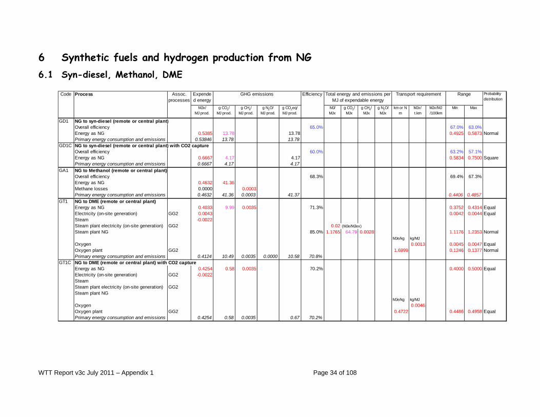
GD1 NG to syn-diesel (remote or central plant)Overall efficiency 65.0% 67.0% 63.0%Energy as NG 0.5385 13.78 13.78 0.4925 0.5873 NormalPrimary energy consumption and emissions 0.53846 13.78 13.78
GD1C NG to syn-diesel (remote or central plant) with CO2 captureOverall efficiency 60.0% 63.2% 57.1%Energy as NG 0.6667 4.17 4.17 0.5834 0.7500 SquarePrimary energy consumption and emissions 0.6667 4.17 4.17
GA1 NG to Methanol (remote or central plant)Overall efficiency 68.3% 69.4% 67.3%Energy as NG 0.4632 41.36Methane losses 0.0000 0.0003Primary energy consumption and emissions 0.4632 41.36 0.0003 41.37 0.4406 0.4857
GT1 NG to DME (remote or central plant)Energy as NG 0.4033 9.99 0.0035 71.3% 0.3752 0.4314 EqualElectricity (on-site generation) GG2 0.0043 0.0042 0.0044 EqualSteam -0.0022Steam plant electricity (on-site generation) GG2 0.02 (MJe/MJex)Steam plant NG 85.0% 1.1765 64.79 0.0028 1.1176 1.2353 Normal
MJe/kg kg/MJOxygen 0.0013 0.0045 0.0047 EqualOxygen plant GG2 1.6999 0.1246 0.1377 NormalPrimary energy consumption and emissions 0.4124 10.49 0.0035 0.0000 10.58 70.8%
GT1C NG to DME (remote or central plant) with CO2 captureEnergy as NG 0.4254 0.58 0.0035 70.2% 0.4000 0.5000 EqualElectricity (on-site generation) GG2 -0.0022SteamSteam plant electricity (on-site generation) GG2Steam plant NG
MJe/kg kg/MJOxygen 0.0046Oxygen plant GG2 0.4722 0.4486 0.4958 EqualPrimary energy consumption and emissions 0.4254 0.58 0.0035 0.67 70.2%
Probability distribution
RangeTransport requirementEfficiency Total energy and emissions per MJ of expendable energy
Assoc. processes
GHG emissions

WTT Report v3c July 2011 – Appendix 1 Page 35 of 108
GD1 NG to syn-diesel plant (GTL) This is the so-called GTL process including NG reforming or partial oxidation followed by the Fischer-Tropsch (FT) synthesis. The plant also includes hydrocracking of the FT product. GTL is a relatively new technology, and we can expect that with continued development the process efficiency will improve. We expect plants designed in the next few years to have a typical overall efficiency of 65% [Source: Shell, SasolChevron], slightly higher than in the 63% assumed in version 2c of this study. This means that 100 MJ of NG in will deliver 65 MJ of combined product, 35 MJ being expended in the process. The selectivity of the process for a specific product can be adjusted to a large degree, notably with a hydrocracking step after the FT synthesis. The maximum practically achievable diesel yield (including the kerosene cut) is considered to be around 75% of the total product, the remainder being mainly naphtha and some LPG. In this case we assume that the plant is built for the primary purpose of producing diesel. Many future plants will not produce any specialties such as base oils and waxes as these markets will soon be saturated. Naphtha and LPG are also potential automotive fuels. The energy required to produce them from refineries is of the same order of magnitude as diesel. The GTL process produces all these products simultaneously but, contrary to the refinery case, there is no technical argument for allocating proportionally more or less energy to one product than to the others (a yield change between e.g. naphtha and diesel would not significantly affect the overall energy balance of the process). We have therefore considered that allocation on energy content basis between the different co-products is a reasonable simplifying assumption if this case and assumed that all products are produced independently with the same energy efficiency. GD1C NG to syn-diesel plant with CO2 capture The "chemical" CO2 from the reforming or partial oxidation reactions and the CO-shift reaction (required to adjust the hydrogen/CO ratio) is scrubbed from the syngas feed to the FT process. The solvent absorption processes commonly used for this purpose produce a virtually pure CO2 stream so that only compression is required for potential transport (and eventual storage). Most GTL plants will be built near gas or oil fields where the CO2 can be re-injected. For FT liquids from NG there is not literature source where a NG FT plant with and without CCS is compared. FT plants are very complex. The layout differs from licensor to licensor and this can have a large impact on the energy penalty for CCS. [IEA 2005] suggests an energy efficiency penalty of 3%. We have used this figure as a basis for our calculation, starting from an overall plant efficiency of 63% in the base case. The CO2 generated in the auxiliary power plant is not recovered in this scheme, so that the CO2 recovery is relatively low at around 75%. GA1 NG to methanol plant The plant energy efficiency selected here corresponds to a current state-of-the-art installation [Statoil 1998]. The upper value (29.64 GJ/t of methanol) is the value guaranteed by the manufacturer, the lower value (28.74 GJ/t of methanol) is a measured value for the methanol plant located in Tjeldbergodden in Norway. This process is applicable to both a remote plant and a large “central” plant located in Europe.

WTT Report v3c July 2011 – Appendix 1 Page 36 of 108
GT1 NG to DME plant There is limited data available on DME and there are no full scale commercial plants on the ground at the moment. The data used here is from Haldor Topsoe [Haldor Topsoe 2002], the main proponent of DME. This process is applicable to both a remote plant and a large “central” plant located in Europe. In both cases electricity is deemed to be produced by a dedicated gas-fired power plant (CCGT, see process GG2). GT1C NG to DME plant with CO2 capture CO2 formed during the steam reforming process is produced in nearly pure form (see process GD1C above) and removed before the synthesis step. Capture is therefore relatively easy and cheap. The figures used here have been derived from [IEA 2005], [Haldor Topsoe 2001], [Haldor Topsoe 2002]. The resulting extra energy consumption for CCS is, however, very low and these figures should be taken with great caution. 6.2 Natural gas to hydrogen
Code Process Expended
energyMJx/
MJ prod.g CO2/
MJ prod.g CH4/
MJ prod.g N2O/
MJ prod.g CO2eq/MJ prod.
MJ/MJx
g CO2/MJx
g CH4/MJx
g N2O/MJx
km or N m
MJx/t.km
MJx/MJ /100km
Min Max
GH1a NG to hydrogen (reforming, on-site, 2 MW hydrogen)NG comp. (0.4 to 1.6 MPa), electricity (EU-mixZ7b 0.0059Energy as NG 0.4406 0.0159 0.4118 0.4694 NormalCO2 emissions EU-mix quality 81.19 0.0705 0.0842 Normal Russian quality 79.30Electricity (EU-mix, LV) 0.0161Primary energy consumption and emissions 0.5037 0.4749 0.5325 EU-mix quality 83.85 84.54 Russian quality 81.95 82.65
GH1b NG to hydrogen (reforming, central plant, 100-300 MW hydrogen)Energy as NG (Russian gas quality) 0.3150 72.38 0.0159 72.78 76.0% 0.289 0.341 Normal
GH1bC NG to hydrogen (reforming, central plant, 100-300 MW hydrogen) with CO2 captureEnergy as NG (Russian gas quality) 0.3650 11.86 0.0159 12.26 73.3% 0.338 0.3920 Normal
Assoc. processes
GHG emissions Efficiency Total energy and emissions per MJ of expendable energy
Probability distribution
RangeTransport requirement
GH1a NG to hydrogen (steam reforming, on-site, 2 MW hydrogen,) GH1b NG to hydrogen (steam reforming, central plant, 100-300 MW hydrogen) The efficiency of the steam reforming proper is largely independent of the size of the plant. In a large plant, however, there are opportunities for optimisation of heat recovery. In this case we have assumed that, in the larger plant, waste heat is recovered to produce electricity, the surplus of which is exported to the grid (substituting EU-mix quality). This results in a much improved overall efficiency in the case of the central plant. The figures used here are from a conceptual plant design [Foster Wheeler 1996]. In the first version of this report we based the NG-to-hydrogen pathway on [Linde 1992]. The latter involved a larger NG input but also surplus electricity production. Taking the appropriate credit into account the net energy balance falls within 1% of the Foster Wheeler case.

WTT Report v3c July 2011 – Appendix 1 Page 37 of 108
GH1bC NG to hydrogen (steam reforming, central plant, 100-300 MW hydrogen) with CO2 capture Steam reforming of natural gas followed by the CO-shift reaction produces a mixture of hydrogen and CO2 with some residual CO as well as unconverted methane. Depending on the purity requirement of the hydrogen, the CO2 is either separated from the hydrogen chemically by solvent absorption or physically using molecular sieves in a Pressure Swing Absorption (PSA) unit [Foster Wheeler 1996].

WTT Report v3c July 2011 – Appendix 1 Page 38 of 108
7 LPG and ethers
Code Process Expended energy
MJx/MJ prod.
g CO2/MJ prod.
g CH4/MJ prod.
g N2O/MJ prod.
g CO2eq/MJ prod.
MJ/MJx
g CO2/MJx
g CH4/MJx
g N2O/MJx
km or N m
MJx/t.km
MJx/MJ /100km
Min Max
LR1 LPG productionEnergy as LPG 0.0529 3.47 0.0500 0.0700 EqualElectricity GG2 0.0028Primary energy consumption and emissions 0.0580 3.75 0.0000 0.0000 3.76
BU1 n-butane to isobuteneElectricity Z7a 0.0022NG for steam (90% eff.) Z6b 0.1627 10.27 0.0325 0.0000 11.08Hydrogen -0.0196Credit for hydrogen produced by NG steam ref. -0.0258 -1.42 -0.0003 0.0000 -1.43Primary energy consumption and emissions 0.1430 9.11 0.0328 0.0000 9.93
EH1 Isobutene + ethanol to ETBEIsobutene BU1 0.7000Ethanol 0.3640Electricity Z7a 0.0010NG Z6b 0.0240Primary energy consumption and emissions 0.0028 0.1194 0.0003 0.0000 0.13
MH1 Isobutene + methanol to MTBEIsobutene BU1 0.8122Methanol 0.1886Electricity Z7a 0.0012NG Z6b 0.0290Primary energy consumption and emissions 0.0028 0.1194 0.0003 0.0000 0.13
Assoc. processes
GHG emissions Efficiency Total energy and emissions per MJ of expendable energy
Probability distribution
RangeTransport requirement
LR1 LPG production It is assumed here that LPG is produced as part of the heavier hydrocarbons (condensate) associated with natural gas. Energy is required for cleaning the gas and separating the C3 and C4 fractions. Reliable data is scarce in this area and this should only be regarded as a best estimate. BU1 n-butane to isobutene This process of isomerisation and dehydrogenation is required to produce isobutene, one of the building blocks of MTBE or ETBE. It is an energy-intensive process. EH1 ETBE manufacture (large plant) This process describes the manufacture of ETBE from isobutene and ethanol. This could occur in Europe with imported butanes (turned into isobutene with BU1) and domestically produced bio ethanol.

WTT Report v3c July 2011 – Appendix 1 Page 39 of 108
MH1 MTBE manufacture (large plant) This represents a typical large scale plant, usually located near a source of natural gas, manufacturing MTBE from isobutene (from field butanes) and methanol (synthesised from natural gas).

WTT Report v3c July 2011 – Appendix 1 Page 40 of 108
8 Synthetic fuels and hydrogen production from coal Expended
energyCode Process MJx/
MJ prod.g CO2/
MJ prod.g CH4/
MJ prod.g N2O/
MJ prod.g CO2eq/MJ prod.
Min Max
KB1 Lignite (brown coal) provisionPrimary energy as Brown coal 0.0148 Oil 0.0008Primary energy consumption and emissions 0.0156 1.77
KO1 Hard coal provision (EU-mix) (1)Primary energy as Hard coal 0.0250 Brown coal 0.0020 Oil 0.0410 Natural gas 0.0100 Hydro power 0.0030 Nuclear 0.0110 Waste 0.0020Primary energy consumption and emissions 0.0940 6.47 0.3818 0.0003 16.10
KH1 Coal to hydrogenEnergy as hard coal (EU-mix) 0.967 188.77 0.0061 50.8%Primary energy consumption and emissions 0.9670 188.77 0.0061 0.0000 188.9254
KH1C Coal to hydrogen with CO2 captureEnergy as hard coal (EU-mix) 1.303 5.64 0.0000 43.4%Primary energy consumption and emissions 1.3030 5.64 0.0000 0.0000 5.638889
KA1 Coal to methanolEnergy as hard coal (EU-mix) 0.6759 91.74 0.0069 91.91 59.7%Electricity (ex coal) 0.0294Primary energy consumption and emissions 0.7371 91.74 0.0069 91.91
KE1 Coal to DMEEnergy as hard coal (EU-mix) 0.6759 93.55 0.0069 93.72 59.7%Electricity (ex coal) 0.0294Primary energy consumption and emissions 0.7371 93.55 0.0069 93.72
KD1 Coal to syndieselEnergy as hard coal (EU-mix) 1.4710 166.31 40.5% 1.3470 1.5950 EqualEnergy as electricity -0.3300Credit for electricity based on coal IGCC -0.6875 -65.98 0.0000 0.0000 -65.98 48%Primary energy consumption and emissions 0.7835 100.33 0.0000 0.0000 100.33 56%
KD1C Coal to syndiesel with CO2 captureEnergy as hard coal (EU-mix) 1.444 14.92 40.9% 1.3220 1.5660 EqualEnergy as electricity -0.239Credit for electricity based on coal IGCC+CCS -0.5829 -5.60 41.0% 50.0% 40.0%Primary energy consumption and emissions 0.8611 9.31 0.0000 0.0000 9.31 54%
(1) Data calculated from composition of current EU-mix and specific energy requirements and efficiencies for each sourceCoal EU-mix as followsSource %Australia 12CIS 3Columbia 7Germany 21Poland 7South Africa 16Spain 6UK 18USA 10
Assoc. processes
EfficiencyGHG emissions Range Probability distribution

WTT Report v3c July 2011 – Appendix 1 Page 41 of 108
KB1 Lignite/brown coal provision This process is typical of brown coal extraction in Germany and Eastern Europe [GEMIS 2002]. Lignite is used as fuel for the ethanol plant in pathways WTET3a/b. KO1 Hard coal provision (EU-mix) These figures approximate the average primary energy associated to the production and provision of hard coal to Europe [El Cerrejon 2002], [DOE 2002], [EUROSTAT 2001], [GEMIS 2002], [IDEAM 2001], [IEA Statistics 2000]. KH1 Coal to hydrogen This represents the total process from coal gasification through CO shift, PSA etc [Foster Wheeler 1996]. KH1C Coal to hydrogen with CO2 capture Same as above with additional capture of CO2. The figures with and without capture are based on a conceptual plant design [Foster Wheeler 1996]. KA1/E1 Coal to methanol or DME This represents the total process from coal gasification through methanol or DME synthesis. The same reference was used for both products [Katofsky 1993]. KD1 Coal to synthetic diesel This is the "CTL" route, including coal gasification and Fischer-Tropsch synthesis [Gray 2001], [Gray 2005], [TAB 1999]. KD1C Coal to synthetic diesel with CO2 capture Same as above with CO2 capture between gasification and FT synthesis [Winslow 2004], [Gray 2001], [Gray 2005], [ENEA 2004].

WTT Report v3c July 2011 – Appendix 1 Page 42 of 108
9 Farming processes Here we tabulate and sum the fossil energy and GHG emissions attributable to farming processes, including the upstream emissions and energy needed to make the fertilizers etc. The related processes for agrochemicals are described in section 10. As explained in the WTT main report, the GHG balances in this report do not include emissions from changes in land use, even though we think these are important. In other words, our figures refer to annual farming emissions, and not to land use change emissions, which should be added separately. However, when we calculate nitrous oxide emissions, we must take into account that soil produces significant “background” N2O emissions even if it is not cultivated. As explained in the WTT main report, the best of a limited range of options is to choose “unfertilized grass” as the land-cover for the calculation of background emissions. This also happens to give a reasonable representation of growing crops on compulsory set-aside land, even though now only a small fraction of the increased crop demand for biofuels targets is considered attainable from abolishing set-aside [DG-AGRI 2007a] All figures are related to the Lower Heating Value of the dry matter (i.e. water-free) of the biomass products. In calculating the lower heating value (LHV), the condensation energy of the water vapour in the flue gas is not counted. In our convention, this arises only from the hydrogen content of the dry-matter. However, some other workers (for example, in the Netherlands) include also the energy for evaporating the water from moist materials. The heat of vaporization is not recovered in the flue gas, so this gives a lower LHV than ours. We do not do this because it causes problems: wood apparently increases in heating value during storage, sewage sludge apparently has a negative LHV, and in the “Dutch” convention energy is not conserved in processes whenever the water content of the products differs from those of the feedstocks. Of course, we take the water content into account when calculating the weight of biomass transported. For easy comparison with other studies, we express agricultural yields in terms of the “conventional” % moisture: 13.5% for EU-wheat; 10% for oilseeds; 9% for DDGS by-product of wheat-ethanol, sugar beet pulp and dried slops (“solubles”); 0% for wood (see complete table on p.12 of this appendix). The primary energy and emissions from diesel use in biomass processes include the LHV and the carbon (as CO2) content of the diesel itself, because the fossil CO2 is released at this stage. Best estimate figures are shown. It is not worth including a range of energy inputs, because these are low for farming compared to the whole chain. The main source of uncertainty is in the GHG emissions, caused by the N2O emission calculation (details in the WTT main report). We call seeds “seeding materials” to avoid confusion with oilseeds as a crop.

WTT Report v3c July 2011 – Appendix 1 Page 43 of 108
Code Process Probabilitydistribution
kg/MJ prod.
MJ/MJ prod.
PrimaryMJx/
kg or MJ
PrimaryMJx/
MJ prod.
g CO2/MJ prod.
g CH4/MJ prod.
g N2O/MJ prod.
g CO2eq/MJ prod.
Min Max
SB1 Sugar Beet FarmingCaO fertilizer AC4 0.0014 2.04 0.0029 0.17 0.0004 0.0000 0.18K2O fertilizer AC3 0.0005 9.73 0.0047 0.26 0.0007 0.0000 0.28P2O5 fertilizer AC2 0.0002 15.47 0.0033 0.21 0.0003 0.0000 0.22N fertilizer AC1 0.0004 49.17 0.0210 1.29 0.0035 0.0041 2.61Pesticides AC5 0.0000 272.55 0.0013 0.08 0.0001 0.0000 0.08Seeding material 0.0000 33.38 0.0007 0.04 0.0000 0.0000 0.04Diesel Z1 0.0226 4.18 0.0262 1.98 0.0000 0.0000 1.98Net emissions from field 0.0001 0.0117 3.48 0.0075 0.0208Farm primary energy consumption and emissions 0.0601 4.03 0.0052 0.0158 8.86…including 4.5% sugar loss during storage 0.0628 4.21 0.0054 0.0165 9.26Yields t/ha/a Sugar beet (dry matter) 17.22
WT1a Wheat farming (grain)K2O fertilizer AC3 0.0002 9.73 0.0021 0.12 0.0003 0.0000 0.13P2O5 fertilizer AC2 0.0003 15.47 0.0044 0.28 0.0004 0.0000 0.29N fertilizer AC1 0.0014 49.17 0.0702 4.31 0.0118 0.0138 8.71Pesticides AC5 0.0000 272.55 0.0083 0.51 0.0008 0.0000 0.53Seeding material 0.0016 2.88 0.0045 0.26 0.0000 0.0000 0.26Diesel Z1 0.0486 4.18 0.0564 4.25 0.0000 0.0000 4.25Net emissions from field 0.0087 2.58 0.0131 0.0043Sum primary energy consumption and emissions 0.1459 9.73 0.0133 0.0224 16.74Yields t/ha/a Wheat grain (13.5% moisture, non-food variety) 5.20 Straw 4.10
WT1b Wheat farming (whole plant)K2O fertilizer AC3 0.0005 9.7284 0.0049 0.27 0.0008 0.0000 0.29P2O5 fertilizer AC2 0.0003 15.4653 0.0050 0.32 0.0004 0.0000 0.33N fertilizer AC1 0.0009 49.1728 0.0419 2.58 0.0071 0.0082 5.20Pesticides AC5 0.0000 272.5524 0.0010 0.06 0.0001 0.0000 0.06Seeding material 0.0007 2.8772 0.0020 0.06 0.0000 0.0000 0.06Diesel Z1 0.0240 1.1600 0.0278 2.10 0.0000 0.0000 2.10Net emissions from field 0.0122 3.64 0.0039 0.0203Sum primary energy consumption and emissions 0.0826 5.39 0.0084 0.0204 11.69
WT1c Double cropping (maize & barley)N fertilizer AC1 0.0003 49.1728 0.0164 1.01 0.0028 0.0032 2.03Diesel Z1 0.0260 1.1600 0.0302 2.28 0.0000 0.0000 2.28Net emissions from field 0.0002 0.0053 1.58Sum primary energy consumption and emissions 0.1815 14.07 0.0195 0.0441 27.70
SC1 Sugar cane farming (Brazil)CaO fertilizer AC4 0.0010 0.5669 0.0020 0.11 0.0003 0.0000 0.12K2O fertilizer AC3 0.0002 2.7023 0.0019 0.11 0.0003 0.0000 0.12P2O5 fertilizer AC2 0.0001 4.2959 0.0012 0.07 0.0001 0.0000 0.08N fertilizer AC1 0.0002 13.6591 0.0083 0.51 0.0014 0.0016 1.03Pesticides AC5 0.0000 75.7090 0.0014 0.09 0.0001 0.0000 0.09Diesel Z1 0.0053 1.1600 0.0061 0.46 0.0000 0.0000 0.46Net emissions from field 0.39 0.0528 0.0067 3.70 0.0027 0.0264Sum primary energy consumption and emissions 0.0210 1.75 0.0550 0.0083 5.61Yields t/ha/a Sugar cane (6-year average) 68.70
WF1 Wood farming and chippingN fertilizer AC1 0.0005 0.0246 1.51 0.0041 0.0048 3.05Diesel for harvest, sowing etc. Z1 0.0060 0.0070 0.53 0.0000 0.0000 0.53Land emissions 0.0034 1.02Diesel for chipping 0.0040 4.18 0.0046 0.35 0.0000 0.0000 0.35Primary energy consumption and emissions 0.0362 2.39 0.0041 0.0082 4.94…including 2.5% dry-mass losses in chipping and storage 0.0371 2.45 0.0042 0.0084 5.07Yields t/ha/a Wood (dry matter) 10.00
N2O emissionsAssoc. processes
Input Expended energy GHG emissions

WTT Report v3c July 2011 – Appendix 1 Page 44 of 108
SB1 Sugar Beet Farming Fertiliser inputs are based on the weighted average of national fertililizer inputs in [EFMA 2008], for countries with sugar-beet ethanol production. They were converted from tonnes/ha to tonnes/MJ of grain using the corresponding yield 68.9 tonnes/ha at 75% moisture. Diesel use per ha was from [FFE 1998] (similar to [ADEME 2003]) and converted to MJ/MJ grain using the same yield. Pesticides/herbicides data are from [Kaltschmitt 1997], amount of seeding material from [FFE 1998]. N2O emissions from the field dominate the GHG emissions. An average for sugar beet grown in EU15 is calculated using the updated JRC soil emissions model, as detailed in the WTT report, section 3.4. We assume that the sugar beet leaves are ploughed back into the soil after harvest, which is the usual practice. In the previous version of this study (2c) we took into account losses of sugar by respiration during storage. However, stakeholders informed us that the quoted sugar beet yield already took into account storage losses, so we eliminated this correction in this version. WT1a-c Wheat Farming Wheat is the highest-yielding cereal crop, but it also takes the highest inputs. This process is for ‘soft wheat’, which accounts for most of EU production, gives the highest yield, and has the highest fermentable content. Straw use is discussed in the main WTT report. As for other crops, fertiliser inputs are based on [EFMA 2008], converted from tonnes/ha to tonnes/MJ of grain using the average EU yield of 5.2 tonnes grain per ha at 13.5% moisture, provided by EFMA. Diesel use per ha was averaged between [Crop Energies 2008] and [ADEME 2002] (which gave similar numbers) and converted to MJ/MJ grain using the same yield. Pesticides/herbicides data are from [Crop Energies 2008], amount of seeding material from [ETSU 1996]. The N2O emissions are calculated by the updated JRC soils emissions model (WTT report, section 3.4). There is no “reference crop” (see main WTT report). In this version we have introduced 3 sub-versions for cereal farming. WT1a represents conventional farming for wheat grain. WT1b represents the case where the whole wheat plant is harvested for biogas production (Pathway OWCG4). WT1c is for a ‘double-cropping’ scenario, where two crops are grown each year with the whole plant being harvested in an immature state, again for production of biogas. In practice, a rotation of maize and barley is more suited to this technique than wheat, and it is this case that has been modelled (Pathway OWCG5). SC1 Sugar cane farming (Brazil) Figures are derived from data for “scenario 2” in the thorough LCA study by [Macedo 2004] which describes best-current-practice in the Centre-South region, where 85% of Brazil’s sugar cane is grown, and where it is claimed there is still plenty of grazing land which could be planted to increase the supply if there is a market. It is a very long way from any rainforest. Some sugar cane is also produced in NE Brazil, near some areas of surviving Atlantic rainforest, but the conditions are much less suitable there, so that production needed subsidies, and is unlikely to increase.
WTT Report v3c July 2011 – Appendix 1 Page 45 of 108
There are usually 5 harvests over a 6 year period, with an average yield of 82.4 t/ha (moist), so the annualized yield is 68.7 t/ha/a. Macedo gives inputs per tonne of moist cane. We converted these to figures per MJ (LHV) dry cane using 72.5% water content of harvested sugar cane [Kaltschmitt 2001] and LHV heat content of 19.6 MJ per kg dry matter [Dreier 2000] (Macedo also describes the process per tonne of cane, so these conversion factors cancel out in the overall calculation). To keep the pathway comparable with other crops, we used our usual chemical processes to calculate the energy and emissions from producing the agricultural inputs, not the values used by Macedo. In this best-practice scenario, the solid “filter mud cake” and liquid “vinasse” residue from the distillation process (equivalent of wet DDGS in the wheat-to-ethanol process) are sent to the closer fields to recycle the water and much of the minerals. The figures represent a weighted average of nearer and more distant fields. The average nitrogen rate over 5 years is about 75 kg/ha. The farming emissions include CO2, methane and nitrous oxide from burning the foliage to make manual harvesting easier. This is still the most common practice, although it is banned near towns. We used Macedo’s calculation of N2O, CH4 and CO2 emissions from burning, using factors recommended in [IPCC 2001]. Nitrous oxide emissions were calculated from the nitrogen fertilizer additions together (in this version) with the nitrogen content of the vinasse and filter cake using IPCC default coefficients. Fortunately they are low, so the related uncertainty is acceptable in this case. Sugar cane resembles more a perennial biomass crop like miscanthus than it does an arable crop. Unlike arable crops in Europe, planting sugar cane on grazing land is believed to actually increase the soil carbon stocks. The risk of soil erosion (a major concern in Brazil) is heightened in the first year of establishment, compared to grazing land, but not in subsequent years. WF1 Wood Farming This represents Short-Rotation Forestry (SRF) on agricultural land. Poplar or willow are generally the best-yielding species in central and Northern Europe. Willow shoots are harvested typically every 3 years; poplar trunks after 8-15 years. After about 15-20 years the trees are uprooted and new ones planted. Inputs comprise sowing, thinning, fertilizers, but mostly harvesting. Yields for a given amount of fertilizer are better than for annual crops because roots are already established at the start of the growing season. Perennial grasses share this advantage. A neutral review of European experiments with miscanthus [Scurlock 1999] indicates a realistic yield similar to farmed wood. Switchgrass has lower yield, but has better drought resistance, enabling it to be grown in more marginal areas. Grasses generally have a higher mineral content than wood, which can cause problems of ash sintering and corrosion if one tries to use the same conversion plant (the salt content can however be lowered by delayed harvesting or washing). For this reason, farmed wood chips command a higher price at power stations, which makes it the preferred biomass crop in Europe at the moment. LCA studies show results for perennial grasses between wood and arable bio-crops. We have considered SRF because there is more data, but do not wish to exclude grasses as a possible alternative with fairly similar characteristics. Inputs vary widely, depending on soil quality, yield and the intensiveness of the farming; [Bauen 2000] gives a range of 0.004 to 0.065 MJ primary energy per MJ dry wood. [Mathews 1994] quotes figures of 0.03 to 0.04 MJ/MJ. Our data on wood farming (short rotation forestry) are from original

WTT Report v3c July 2011 – Appendix 1 Page 46 of 108
Oeko-Institute studies in the [GEMIS 2002] database, used also in [LBST 2002]. Inputs are low compared to other energy crops, so the uncertainty is not important when comparing pathways. Nitrous oxide emissions for forestry cannot be calculated with the JRC soil model. Instead, we used the range of measured values for direct emissions from poplar, reported by [Flesse 1998]. A range for indirect emissions was estimated, using the procedure based on IPCC guidelines described in [LBST 2002], for the 25 kg/ha nitrogen fertilizer rate reported by [Murach 2003] for poplar plantation. Since this procedure assumes that nitrous oxide emissions are proportional to the nitrogen fertilizer rate, the emissions from our reference crop (unfertilized grass) are effectively already subtracted. For the nitrous oxide and farming input calculations, the yield is taken to be 10 tonnes/ha, and the LHV of dry farmed wood (poplar) chips 18 GJ/ dry tonne [GEMIS 2002]. Dry mass losses during chipping and storage are partly from dust and spillage, and partly from respiration, rotting and evaporation of volatiles, in line with [Hamelinck 2002].
Code Process Probabilitydistribution
kg/MJ prod.
MJ/MJ prod.
PrimaryMJx/
kg or MJ
PrimaryMJx/
MJ prod.
g CO2/MJ prod.
g CH4/MJ prod.
g N2O/MJ prod.
g CO2eq/MJ prod.
Min Max
RF1 Rapeseed FarmingCaO fertilizer AC4 0.0003 2.04 0.0005 0.03 0.0001 0.0000 0.03K2O fertilizer AC3 0.0007 9.73 0.0065 0.37 0.0010 0.0000 0.39P2O5 fertilizer AC2 0.0005 15.47 0.0070 0.45 0.0006 0.0000 0.46N fertilizer AC1 0.0019 49.17 0.0914 5.62 0.0154 0.0179 11.34Pesticides AC5 0.0000 272.55 0.0045 0.28 0.0004 0.0000 0.29Seeding material 0.0001 7.14 0.0006 0.02 0.0000 0.0000 0.02Diesel (including drying and storage) Z1 0.0403 4.18 0.0467 3.53 0.0000 0.0000 3.53Net emissions from field 0.0001 0.0419 12.50 0.0272 0.0675 Double triangleDrying & storage electricity (EU mix LV) Z7b 0.0031 10.33 0.0088 0.37 0.0009 0.0000 0.40Sum primary energy consumption and emissions 0.1661 10.66 0.0186 0.0599 28.96Yields t/ha/a Rape seed (dry matter) 2.70
SF1 Sunflower seed FarmingK2O fertilizer AC3 0.0004 9.7284 0.0037 0.21 0.0006 0.0000 0.22P2O5 fertilizer AC2 0.0005 15.4653 0.0080 0.51 0.0007 0.0000 0.53N fertilizer AC1 0.0007 49.1728 0.0331 2.03 0.0056 0.0065 4.10Pesticides AC5 0.0000 272.5524 0.0091 0.55 0.0008 0.0000 0.58Seeding material 0.0001 0.0006 0.02 0.0000 0.0000 0.02Diesel Z1 0.0528 4.1760 0.0613 4.62 0.0000 0.0000 4.62Net emissions from field 0.0002 0.0247 7.37 0.0164 0.0342 Normaldrying (electricity) 0.0031 10.3273 0.0088 0 0.0009 0.0000 0.39Sum primary energy consumption and emissions 0.1245 8.31 0.0087 0.0312 17.84Yields t/ha/a Sunflower seed (10% moisture) 2.44
N2O emissionsAssoc. processes
Input Expended energy GHG emissions

WTT Report v3c July 2011 – Appendix 1 Page 47 of 108
RF1 Rapeseed Farming Rape gives the highest oil yield in the Northern half of Europe. However, it still has much lower yield than cereals: it is typically grown as a low-input break crop, to rest the soil between more profitable cereal crops. The rape straw is invariably ploughed back into the soil, because it contains most of the nitrogen and minerals taken up by the crop and is needed to improve the organic content of the soil. Fertiliser inputs are based on [EFMA 2008], converted from tonnes/ha to tonnes/MJ of grain using the average EU yield of 3.1 tonnes per ha at 10 % moisture, provided by EFMA. Diesel use per ha is from [FfE 1998], (which lies between those in [Groves 2002] and [ADEME 2002]), and is converted to MJ/MJ grain using the same yield. Pesticides/herbicides data are from [UBA 1999], amount of seeding material from [Kaltschmitt 1997]. The N2O emissions are calculated by the updated JRC soils emissions model (WTT report, section 3.4). The dry LHV of rapeseed is 23.8 GJ/t at standard 10% moisture [FfE 1998]. SF1 Sunflower Seed Farming Rapeseed does not grow well in the drier parts of Europe: here, sunflower is grown in rather the same way, in rotation with cereals, although average yields are lower. Inputs are from [FfE 1998], and average EU-15 N2O field emissions are calculated from the JRC soil model. We assume the straw is ploughed in the soil, which is the usual practice. We assumed the same LHV for sunflower seed as for rapeseed. The data from EFMA do not specifically include sunflower as a crop. Therefore our fertiliser inputs are based on [ADEME 2002], converted from tonnes/ha to tonnes/MJ of grain using their yield of 2.44 tonnes/ha at 10 % moisture. Diesel use per ha is from [FfE 1998], and is converted to MJ/MJ grain using the same yield. Pesticides/herbicides data are from [ADEME 2002]. The N2O emissions are calculated by the updated JRC soils emissions model (WTT report, section 3.4). There is no “reference crop” (see WTT report). The dry LHV of rapeseed is 23.8 GJ/t at standard 10% moisture [FfE 1998].

WTT Report v3c July 2011 – Appendix 1 Page 48 of 108
Code Process Probabilitydistribution
kg/MJ prod.
MJ/MJ prod.
PrimaryMJx/
kg or MJ
PrimaryMJx/
MJ prod.
g CO2/MJ prod.
g CH4/MJ prod.
g N2O/MJ prod.
g CO2eq/MJ prod.
Min Max
SY1 Soya bean Farming (Brazil, for oil production)K2O fertilizer AC3 0.0011 9.7284 0.0108 0.61 0.0017 0.0000 0.65P2O5 fertilizer AC2 0.0012 15.4653 0.0183 1.16 0.0015 0.0000 1.20N fertilizer AC1 0.0001 49.1728 0.0070 0.43 0.0012 0.0014 0.86Pesticides AC5 0.0000 272.5524 0.0132 0.80 0.0012 0.0000 0.84Diesel Z1 0.0375 1.1600 0.0435 3.28 0.0000 0.0000 3.28Net emissions from field 0.0397 11.84 0.0147 0.0647 NormalSum primary energy consumption and emissions 0.0927 6.28 0.0057 0.0411 18.68
PO1 Oil palm tree plantation (FFB)K2O fertilizer AC3 0.0007 9.7284 0.0065 0.36 0.0010 0.0000 0.39P2O5 fertilizer AC2 0.0005 15.4653 0.0074 0.47 0.0006 0.0000 0.49N fertilizer AC1 0.0004 49.1728 0.0209 1.28 0.0035 0.0041 2.59Pesticides AC5 0.0000 272.5524 0.0076 0.46 0.0007 0.0000 0.48Diesel Z1 0.0069 1.1600 0.0080 0.60 0.0000 0.0000 0.60Net emissions from field 0.0117 3.48 0.0028 0.0556 Double triangleSum primary energy consumption and emissions 0.0503 3.18 0.0060 0.0158 8.03
CR1 Corn farming Brazil (mass based) kg/kg corn MJ/kg corn
MJ/kg corn
g CO2/kg corn
g CH4/kg corn
g N2O/kg corn
g CO2eq/kg corn
K2O fertilizer AC3 0.0027 9.7284 0.0951 5.35 0.02 0.00 5.73P2O5 fertilizer AC2 0.0029 15.4653 0.1604 10.21 0.01 0.00 10.58N fertilizer AC1 0.0033 49.1728 0.5827 35.81 0.10 0.11 72.28Pesticides AC5 0.0002 272.5524 0.1853 11.30 0.02 0.00 11.77Diesel Z1 1.0267 1.1600 1.1910 89.89 0.00 0.00 89.89Net emissions from field 0.4270 127.25 0.1030 1.9450 Double triangleSum primary energy consumption and emissions 2.2145 152.56 0.1442 0.5414 317.50
N2O emissionsAssoc. processes
Input Expended energy GHG emissions
SY1 Soy Bean Farming Soy bean meal is the main protein-rich animal feed in Europe. Brazil was the main exporter of soy beans to EU until the recent boom in US soy bean-biodiesel, driven by anomalies in biofuels subsidies between US and EU. This is expected to be a transient phenomenon, so we have retained Brazil as the largest source of future soy beans. Data relative to soy bean farming and downstream processes is required for two purposes:
• As was already the case in previous versions of this study, we use soy meal as the notional “swing” source of animal feed i.e. as a basis for substitution calculations of various biofuels co-products (the substitution calculation methodology, which now also involves wheat, is described in section 13.1).
• In this version, we have also included pathways for production of soy bean methyl ester in Europe, which uses the same data (although it now needs to be expressed on an energy basis). Brazil is the largest producer of soy beans and we have modelled production from this source.
WTT Report v3c July 2011 – Appendix 1 Page 49 of 108
Nitrogen fertilizer rates and yields are taken from Brazilian data [FAO 2004] (produced in collaboration with IFA). Pesticide/herbicide application rates are from [Altieri 2005]. Diesel use is from [UBA 1999]. Nitrous oxide emissions are calculated from [IPCC 2006] default values, but the nitrogen content of the below-ground biomass was corrected as described in the main WTT report section 3.4.2. PO1 Palm Oil Plantation Palm oil methyl ester pathways are also a new addition to this version. A general description of palm oil production is given in the WTT Report, Section 3.4.10.
In our calculations, synthetic fertilizer inputs are the recommended use from [FAO 2004], based on replacing nitrogen extracted from the plantation. This nitrogen fertilizer rate is considerably lower than reported by [Teoh 2004], but about the same if we subtract the nitrogen content of the empty palm bunches recycled as mulch. On the other hand, the actual fertilizer use reported by FAO is about 1/3 lower and cannot be reconciled with the [Teoh 2004] data. These data are used as the lower uncertainty limit of average fertilizer use. It may represent farming practice close to the mill where there is an excess of mulch available from other growers’ palm bunches, or it includes plantations where soil nitrogen has been allowed to fall, and will need to be made up at some point in the future if yields are to be maintained. Another possibility is that the average is lowered by including plantations on drained peat, which need less synthetic nitrogen because of nitrogen mineralized as a result of the decay of organic matter in the soil. Pesticides and diesel use are from [Teoh 2004]. As cited by [S&T Consultants 2007] nitrous oxide emissions were calculated from the nitrogen content of synthetic fertilizer and mulch using [IPCC 2006] guidelines. We think this is probably an underestimate for the part of palm oil grown on drained peat. We do not include the very high emissions of CO2 (and N2O) due to decay of peat, since they are due to land use change. However, if synthetic N fertilizer or organic mulch is also applied, the acidic, high-organic, soil is very likely to convert a much larger proportion of the additional nitrogen to N2O than indicated by the default emission factor in the IPCC guidelines we have used. CR1 Corn farming This new process is provided for the calculation of credit for soy meal production (see section 13.1) in process SY3b (section 13.5). Figures are based on available data for corn farming in Romania (under the assumption that farming input are similar in other parts of the world).

WTT Report v3c July 2011 – Appendix 1 Page 50 of 108
N2O EMISSIONS CALCULATION FOR ARABLE CROPS Nitrous oxide emissions dominate the greenhouse gas emissions from farming, and are important for all biomass-based pathways. Therefore we were careful to use the best possible estimate of EU emissions. The IPCC guidelines are highly simplified and therefore need a very wide error range. The method used by JRC to estimate average GHG emissions for the different biofuels crops is described in the main WTT report, section 3.4.2. This is for EU-15, but we expect the average nitrous oxide emissions per MJ crop produced to be similar for EU-25. The method could not be used for short-rotation forestry, sugar cane farming or oil palms because these crops are not covered in the DNDC soils model we used. Here, we were forced to use IPCC default emission factors [IPCC 1996/1] which estimated nitrous oxide emissions based on nitrogen fertilizer rates. Soy beans are also not covered by the JRC model for EU. However, the results using the IPCC (tier 1) methodology hugely changed from the 1996 guidelines and the 2006 guidelines. Investigating the subject in detail, our colleagues at E4Tech in the UK found that the IPCC 2006 guidelines were seriously in error for leguminous plants in general and for soy beans in particular. We checked their reasoning, and agree with them, as explained in WTT report section 3.4.2. Therefore our best estimate of N2O emissions from soy bean farming uses a corrected form of the 2006 IPCC guidelines, which gives a result between that of the 1996 and 2006 IPCC tier 1 guidelines.

WTT Report v3c July 2011 – Appendix 1 Page 51 of 108
10 Production of agro-chemicals All data on fertilizer and fuel inputs for agro-chemicals provision come from [Kaltschmitt 1997]. These data include the transport of the fertilizer. In these processes, the “MJ primary energy per MJ input” of fuel inputs includes the LHV and fossil carbon (as CO2) content of the fuel itself, as well as the upstream energy/emissions to make it. However, [Kaltschmitt 1997] do not include upstream energies and emissions, so our figures are moderately higher, especially where a lot of electricity is used. Our primary energies are similar to those in the new [ADEME 2003] report.
Code Process Inputkg/
kg prod.As used
MJ/kg prod.
MJx/MJ
PrimaryMJx/
kg prod.
g CO2/kg prod.
g CH4/kg prod.
g N2O/kg prod.
g CO2eq/kg prod.
AC1 Nitrogen Fertilizer Provision (as N)Electricity (EU-mix, MV) Z7a 0.6 2.83 1.78 74.8 0.18 0.0034 80.3Hard coal KO1 3.9 1.09 4.32 404.6 1.51 0.0011 442.6Diesel Z1 0.9 1.16 1.00 75.3 0.00 0.0000 75.3Heavy fuel oil Z3 4.4 1.09 4.77 384.1 0.00 0.0000 384.1NG Z6b 33.0 1.13 37.31 2083.0 6.58 0.0008 2247.8N2O from process 9.6300Primary energy and emissions/kg 49.17 3021.7 8.27 9.6353 6099.9
AC2 P fertilizer provision (as P2O5)Electricity (EU-mix, MV) Z7a 1.6 2.83 4.54 191.2 0.47 0.0086 205.4Hard coal KO1 0.6 1.09 0.62 58.4 0.22 0.0002 63.9Diesel Z1 1.1 1.16 1.30 98.1 0.00 0.0000 98.1Heavy fuel oil Z3 5.0 1.09 5.44 438.3 0.00 0.0000 438.3NG Z6b 3.2 1.13 3.56 198.8 0.63 0.0001 214.6Primary energy and emissions/kg 15.47 984.8 1.31 0.0089 1020.3
AC3 K fertilizer provision (as K2O)Electricity (EU-mix, MV) Z7a 0.2 2.83 0.62 26.2 0.06 0.0012 28.2Diesel Z1 0.5 1.16 0.63 47.3 0.00 0.0000 47.3NG Z6b 7.5 1.13 8.48 473.4 1.50 0.0002 510.8Primary energy and emissions/kg 9.73 546.9 1.56 0.0014 586.3
AC4 CaO fertilizer provision (85%CaCO3+15%CaO,Ca(OH)2)Electricity (EU-mix, MV) Z7a 0.4 2.83 1.13 47.7 0.12 0.0022 51.2Coal KO1 0.3 1.09 0.35 33.2 0.12 0.0001 36.3Diesel Z1 0.2 1.16 0.21 16.2 0.00 0.0000 16.2NG Z6b 0.3 1.13 0.34 18.9 0.06 0.0000 20.4Primary energy and emissions/kg 2.04 116.0 0.30 0.0023 124.2
AC5 Pesticides (etc) provisionElectricity (EU-mix, MV) Z7a 28.5 2.83 80.72 3398.9 8.29 0.1535 3651.9Hard coal KO1 7.6 1.09 8.35 781.8 2.91 0.0021 855.3Diesel Z1 58.1 1.16 67.40 5086.9 0.00 0.0000 5086.9Heavy fuel oil Z3 32.5 1.09 35.37 2849.9 0.00 0.0000 2849.9NG Z6b 71.4 1.13 80.71 4505.9 14.24 0.0018 4862.5Primary energy and emissions/kg 272.55 16623.4 25.45 0.1573 17306.4
Expended energy GHG emissionsAssoc.processes
Nitrogen fertilizer inputs are quoted per kg N, whereas the others are expressed per kg P2O5, K2O or CaO equivalent (in practice the active ingredient may actually be present in a mixture of compounds). The kg/MJ inputs of fertilizer to the farming processes use the same convention.

WTT Report v3c July 2011 – Appendix 1 Page 52 of 108
AC1-3 N/P/K Fertilizer Provision Nitrogen fertilizer is the main source of GHG emissions from agro-chemicals manufacture. Most of the GHG emissions come from N2O released from the process itself. We thoroughly reviewed data contributed by stakeholders, but found internal inconsistencies for which we could not obtain a satisfactory explanation. Therefore we continue to use the values in [Kaltschmitt 1997] used in previous versions of this study. These figures are also consistent with those in [ECFIN DG241]. In the future, we hope that the data submission in the context of the EU Emission Trading Scheme will provide us with reliable updated industry-average figures. AC4 Lime (CaO+CaCO3) Provision Lime contains roughly 85 % m/m CaCO3 and 15% CaO, partially hydrated to Ca(OH)2. When used as a fertilizer, the CaO content neutralizes the carbonic acid produced by decaying vegetable matter. This carbonic acid would otherwise release its CO2 to the air. Therefore the CO2 produced by the calcining process (“process emissions” in [Kaltschmitt 1997]) is later effectively reabsorbed and should be left out of GHG calculations. Lime requirements for a particular crop vary greatly depending on soil type. Fortunately, though, it never represents a major energy input to our farming pathways, so the effect of the uncertainty is small. AC5 Provision of other farming inputs This comprises all complex organic compounds used in the farming processes such as pesticides, fungicides, plant hormones etc. The input energy and emissions data (from [Kaltschmitt 1997]) are necessarily a very approximate guess. [ADEME 2003] give a range of 175-576 MJ/kg primary energy for various “plant health products”. Our value of 266 MJ/kg compares well with their best-estimate of 297 MJ/kg. Our emissions are considerably higher than those calculated by [Kaltschmitt 1997] from the same data (they may have overlooked the process emissions). The final fate of the carbon in the pesticides themselves is uncertain, but the amount of CO2 involved is negligible. In fact, in general, the mass of pesticides in farming processes is so small that the choice of data has negligible effect on the total farming emissions.

WTT Report v3c July 2011 – Appendix 1 Page 53 of 108
11 Biomass transport
Code Process Assocprocesses
one-w aydistance
km
t.km/MJ prod.
MJ diesel/t.km
MJx/t.km
gCO2eq/t.km
MJx/MJ prod.
gCO2eq/MJ prod.
LossMJ/MJ
Standard biomass transportersZ8a 40 t truck for dry product (round trip considered)
Diesel Z1,Z2 0.94 1.09 81.95Z8b 12 t truck for dry product (round trip considered)
Diesel Z1,Z2 2.01 2.01 176.18Z10 Ocean-going bulk carrier
Fuel oil Z3 0.20 0.22 17.77Solid biomass road transportWC2a Wood chips road transport, 50 km Z8a 50 0.004 0.94 1.09 81.95 0.0043 0.33 0.000WC2b Wood chips road transport, 12 km Z8a 12 0.001 0.94 1.09 81.95 0.0010 0.08 0.000SB2 Sugar beet road transport Z8a 50 0.013 0.94 1.09 81.95 0.0142 1.07 0.000WT2a Wheat grain road transport Z8a 50 0.003 0.94 1.09 81.95 0.0037 0.28 0.010WT2b Wheat straw road transport Z8a 50 0.003 0.94 1.09 81.95 0.0038 0.28 0.000WT2c Wheat whole plant road transport Z8a 20 0.001 0.94 1.09 81.95 0.0015 0.11 0.000SC2 Sugar cane road transport Z8a 20 0.004 0.94 1.09 81.95 0.0040 0.30 0.000RO2 Rapeseed road transport Z8a 50 0.002 0.94 1.09 81.95 0.0023 0.17 0.010SO2 Sunflower seed road transport Z8a 50 0.002 0.94 1.09 81.95 0.0023 0.17 0.010PO2 Palm FFB road transport Z8a 50 0.003 2.01 1.09 176.18 0.0034 0.56 0.020SY2 Soya bean road transport (Brazil) Z8a 700 0.126 0.94 1.09 81.95 0.1368 10.33Solid biomass shippingWC2c Coastal/river shipping wood chips Z8a 400 0.034 0.43 0.50 37.76 0.0171 1.29 0.000Manure transportBG1a Liquid manure transport, 10 km Z2 10 0.013 0.94 1.09 81.95 0.0146 1.10BG1b Dry manure transport, 10 km Z2 10 0.004 0.94 1.09 81.95 0.0047 0.35Long-distance biofuel transportSC4a Sugar cane ethanol road transport to port Z2 700 0.028 0.94 1.09 81.95 0.0305 2.31PO4a Palm oil road transport to port Z2 150 0.004 0.94 1.09 81.95 0.0048 0.36
Naut. MilesSC4b Sugar cane ethanol shipping from Brazil Z4 5500 0.380 0.0512 4.11PO4b Vegetable oil shipping Z4 5500 0.275 0.0371 2.75

WTT Report v3c July 2011 – Appendix 1 Page 54 of 108
Z8a 40 tonne truck for dry products This corresponds to the nominal 23 t payload truck from [ESU 1996], consistent with EURO IV emissions limits. Fuel consumption takes an empty return trip into account. The actual payload depends on the density of the material. This is taken into account when calculating effective t.km in each individual trucking process. According to [Kaltschmitt 2001] such a truck can actually carry up to 27 t for dense material, but for biomass the capacity is often limited by the maximum volume, which is 100 m3. For rapeseed, for example, the actual payload is 22 t, close to the nominal payload. This module is used for all pathways that use truck transport, unless otherwise stated. Z8b 12 tonne truck for dry products For transport of palm oil FFB we modelled a smaller truck, which consequently has higher fuel consumption per t.km. Z10 Ocean-going bulk carrier This represents a 40,000 t dry product carrier. Heavy fuel oil consumption is from [Kaltschmitt 1997]. The calculation methodology is the same as for liquid transport (see above). BIOMASS TRANSPORT DISTANCES FARMED WOOD For a catchment area shaped like our map, 50 km average transport distance gives access to about 0.6 Mha. If we assume 50% of this area is arable land, and 10% of this arable land is farmed wood, with a yield of 10 dry t/ha, then annual production from the catchment area is 300 dry kt. A 10 MW plant (based on feed) requires 16.8 dry kt wood per year (at 18 GJ/t). By quadratic scaling, we need an average transport distance of 12 km. For a 200 MW plant we need 336 dry kt wood per year; implying a single catchment area with an average transport distance of about 50 km. STRAW In the good wheat-growing areas where straw may be harvested, the straw yield from wheat is about 5 t/ha. But these are prime agricultural areas with a high proportion of cereals farms. If we assume 60% of the land is arable, and 70% of that grows wheat (or other suitable cereals), then the transport distance is reduced to 25 km for a 200 MW plant. Note that the projected Iogen plant is about 150 MW. FOREST RESIDUALS The Pietarsaari cogeneration plant in Finland collects up to 200,000 m3 forestry residues per year, with a maximum transport distance of 80 km [TEKES 2002]. That means 90 dry kt/a for a dry-matter density of 0.4 dry t/m3. The average transport distance would then be about 50 km. These forestry residues give a total dry matter LHV energy input of 54 MW. For a 200 MW plant, for example on
50 km average transport distance
WTT Report v3c July 2011 – Appendix 1 Page 55 of 108
the Baltic coast, one would need to ship wood in from about 4 collecting points like this. Considering the geography of the Baltic this would correspond to maybe 400 km average shipping distance. A central-European scenario, with barge transport on the Rhine or Danube, gives similar results. For a 10 MW plant, we get about 12 km road transport distance by quadratic scaling from the Pietarsaari example. BIOENERGY-CROPS In the literature one can find transport distances from the farm gate to the processing plant anywhere from 10 to almost 200 km. The lower end represents theoretical calculations of the radius needed to grow sufficient crop to feed the factory, on the assumption that all farmers cooperate. The second represents the actual trucking distance for some existing plants: their supplies come from scattered farms which have opted to grow designated energy crops under existing rules for agricultural subsidies. Our distance represents what we think is reasonable for the medium-term future, if energy farming becomes much more common. The calculation of t.km per MJ product takes into account the real payload of the truck, bearing in mind the volume limitation of the truck (see trucking processes). The return journey is already taken into account in the truck fuel consumption. For finely divided materials, 1% losses during loading and transport are considered. MANURE This is used for biogas, usually at fairly small scale, hence the short transport distance taken into account. SY2 Soy bean transport As explained in WTT report section 3.4.10 we have assumed that whole beans are transported to Europe where crushing takes place. However the extra soy meal available in Europe as a result replaces soy meal that we otherwise be imported so that the transport cost of the meal is cancelled out. As a result the transport vectors in the soy biodiesel pathways consist in soy bean road transport within Brazil (700 km) and sea shipping of oil only (5500 nautical miles, see PO4b below).The crushing plant is notionally located at an EU port and uses European energy vectors. As mentioned in section 9, SY1 soy meal is also used for calculating animal feed credits in other pathways. Everything in this pathway is related to mass of soy meal, since animal feed replacements are calculated in terms of mass, not lower heating value. PO2 Palm FFB The fresh fruit bunches are transported about 50 km to the crushing plant. Stakeholders told us that transport of the FFB takes place using fairly small trucks. We assumed 12 tonne trucks with 7 tonne payloads, and hence relatively high fuel consumption per tonne-km (Z8b).

WTT Report v3c July 2011 – Appendix 1 Page 56 of 108
PO4a Palm oil road transport After crushing the oil is transported 150 km by road to the port in 40 t trucks (Z8a). PO4b Vegetable oil shipping For sea transport of oil to Europe, we used a generic distance of 5500 nautical miles.

WTT Report v3c July 2011 – Appendix 1 Page 57 of 108
12 Biogas from organic materials 12.1 Biogas from organic waste Three sources of organic waste are considered namely municipal waste, "liquid" manure and dry manure. The process is described in the main WTT report. The anaerobic fermentation produces raw biogas that, depending on the intended use, may need to be treated (to remove contaminants such as sulphur) and/or upgraded (to remove CO2). The plant usually produces its own heat and electricity (CHP). Data for municipal waste is from [Börjesson 2004], [Börjesson 2005] and from [Boisen 2005] for manure. All three options include a small credit for use of the residual organic material as fertiliser. When left untreated, stored manure produces methane that is vented to the atmosphere. This is particularly so for liquid manure where the right conditions for anaerobic fermentation are met. Using manure for biogas production therefore offers a credit for avoided “field” methane emissions. This should be larger for liquid manure than solid, but we only have an average figure.

WTT Report v3c July 2011 – Appendix 1 Page 58 of 108
Bio-feed
MJ bio-en/MJ prod.
As usedMJ/
MJ prod.
MJx/MJ
PrimaryMJx/
MJ prod.
g CO2/MJ prod.
g CH4/MJ prod.
g N2O /MJ prod.
g CO2eq /MJ prod.
Min Max
Raw biogas production from municipal wasteMunicipal waste 1.4286 70% 1.2286 1.6286 SquareHeat (for info, internally generated) 0.0865 0.0778 0.0952 SquareElectricity (for info, internally generated) 0.0622 0.0311 0.0933 SquareMethane losses 0.2000Raw biogas production from liquid manureMunicipal waste 1.4286 70% 1.2286 1.6286 SquareHeat (for info, internally generated) 0.1500 0.1400 0.1700 SquareElectricity (for info, internally generated) 0.0430 0.0400 0.0500 SquareMethane losses 0.2000Methane field emissions credit -2.8571 -1.4286 -4.2857Raw biogas production from dry manureMunicipal waste 1.4286 70% 1.2286 1.6286 SquareHeat (for info, internally generated) 0.1500 0.1400 0.1700 SquareElectricity (for info, internally generated) 0.0430 0.0400 0.0500 SquareMethane losses 0.2000Methane field emissions credit -0.2857 -0.1429 -0.4286Biogas treatment and upgrading Raw biogas 1.0100Electricity (for info, internally generated) 0.0300 0.0200 0.0400 SquareMethane losses 0.2000Biogas CHP plantRaw biogas 1.7000 1.6150 1.7850 SquareHeat generation -1.0000Electricity generation -0.5000Methane losses 0.0533Raw biogas to electricity (small scale, local)Raw biogas 2.5000 2.3800 2.6200 SquareHeat generation -1.2500Electricity generation -1.0000Methane losses 0.0778
Code Process Assoc. processes
Expended energy Probability distribution
GHG emissions Range
Heat and power generation in the biogas plant Power generation is carried out using a gas engine driving an electrical generator. Where the primary product is biogas, only a small part of the biogas is used in the CHP plant, and the electrical efficiency is 29%. Where the whole biogas production is used to generate electricity a larger engine/generator can be used, with an electrical efficiency of 40%.

WTT Report v3c July 2011 – Appendix 1 Page 59 of 108
Bio-feed
MJ bio-en/MJ prod.
As usedMJ/
MJ prod.
MJx/MJ
PrimaryMJx/
MJ prod.
g CO2/MJ prod.
g CH4/MJ prod.
g N2O /MJ prod.
g CO2eq /MJ prod.
Min Max
BG2a Municipal waste to biogas (upgraded)Municipal waste 1.6915 0.6915Electricity import Z7a 0.0524 2.8347 0.1486 0.00Methane losses 0.4461N-fertiliser credit -0.0314 -3.90Primary energy consumption and emissions 0.8087 0.4408 7.25
BG2b Liquid manure to biogas (upgraded)Liquid manure 1.9346 0.9346Electricity import Z7a -0.0133 2.8347 -0.0378 0.00Methane losses 0.4893 12.23Methane field emissions credit -3.8693 -96.73N-fertiliser credit -0.0222 -2.75Primary energy consumption and emissions 0.8746 -3.3837 -87.25
BG2c Dry manure to biogas (upgraded)Dry manure 1.9346 0.9346Electricity import Z7a -0.0133 2.8347 -0.0378 0.00Methane losses 0.4893 12.23Methane field emissions credit -0.3869 -9.67N-fertiliser credit -0.0222 -2.75Primary energy consumption and emissions 0.8746 0.0986 -0.20
BG3a Municipal waste to electricity (small scale, local) Municipal waste 4.2287 3.2287Heat surplus (for info, no credit given) -1.2241Methane losses 0.6843 17.11N-fertiliser credit -0.0786 -9.75Primary energy consumption and emissions 3.1501 0.6710 7.36
BG3b Liquid manure to electricity (small scale, local) Liquid manure 4.0011 3.0011Heat surplus (for info, no credit given) -0.9809Methane losses 0.6475 16.19Methane field emissions credit -8.0022 -200.06N-fertiliser credit -0.0459 -5.69Primary energy consumption and emissions 2.9552 -7.3624 -189.56
BG3c Dry manure to electricity (small scale, local) Dry manure 4.0011 3.0011Heat surplus (for info, no credit given) -0.9809Methane losses 0.6475 16.19Methane field emissions credit -0.8002 -20.01N-fertiliser credit -0.0459 -5.69Primary energy consumption and emissions 2.9552 -0.1604 -9.51
Code Process Assoc. processes
Expended energy Probability distribution
GHG emissions Range
BG2 Waste biomass to upgraded biogas Processes BG2a/b/c represent the integration of these steps to produce upgraded biogas from the different feedstocks. This gas is then suitable to be introduced into a natural gas grid. In principle, it could also be compressed and used as a vehicle fuel, but this step is not included here. Electricity and

WTT Report v3c July 2011 – Appendix 1 Page 60 of 108
heat for the plant needs are generated on site, with a small excess of electricity exported. There is a fertilizer credit from the use of digester residues on the fields. BG3 Waste biomass to electricity (small scale) Processes BG3a/b/c follow the same form, but all the biogas is used to produce electricity. The upgrading step is not needed, since the gas engine is tolerant of some impurities in the fuel. 12.2 Biogas from crops While waste is the most economic source of biomass, biogas digesters can in principle handle a wide range of organic material. In these pathways we explore the options of using cereal crops to produce biogas as an alternative to ethanol. A key difference between the two routes is that, for biogas production, the whole plant, rather than just the grain can be used. WB1 Whole wheat to biogas (upgraded)
Wheat (whole plant) 2.0314Heat (self-generated in CHP) 0.1590Electricity (self-generated in CHP) 0.029Electricity surplus credit -0.0094 2.8347 -0.0267 -1.12 0.00 0.00 -1.21Fertilizer credit kg/MJ prod.
N -0.0017 -0.0824 -5.06 -0.01 -0.02 -10.22 P2O5 -0.0004 -0.0061 -0.39 0.00 0.00 -0.40 K2O -0.0010 -0.0099 -0.56 0.00 0.00 -0.60Methane losses 0.20 5.00Primary energy consumption and emissions -0.1250 -7.13 0.18 -0.02 -7.42
WB2 Double cropping (maize and barley) (upgraded)Wheat (whole plant) 2.1384Heat (self-generated in CHP) 0.1590Electricity (self-generated in CHP) 0.0290Electricity surplus credit -0.0125 2.8347 -0.0355 -1.49 -0.0036 -0.0001 -1.60Fertilizer credit kg/MJ prod. 0 0.00 0.0000 0.0000 0.00 N -0.0004 -0.0210 -1.29 0.00 0.00 -2.61Methane losses 0.20 5.00Primary energy consumption and emissions -0.0565 -2.79 0.19 0.00 0.79Biogas CHP plantBiogas 1.7000Heat 1.0000Power 0.5000

WTT Report v3c July 2011 – Appendix 1 Page 61 of 108
WB1 Whole wheat to biogas Wheat is grown to maturity in the normal way and the whole plant (grain and straw) is used in a biogas digester. The residue is used on the fields, reducing fertilizer requirements. A small part of the gas is used to produce electricity and heat for the plant, with the excess electricity being exported. The remainder of the gas is cleaned and upgraded so that it can be fed into the natural gas grid. WB2 Double cropping whole plant maize and barley to biogas This process is similar to WB1 except for the source of biomass. Two crops are grown each year, with the whole plant being harvested perhaps before it reaches maturity. In European conditions, maize and barley look the best crops for this purpose where the objective is simply to maximise the amount of biomass produced.

WTT Report v3c July 2011 – Appendix 1 Page 62 of 108
13 Conversion processes for “conventional biofuels” The range of energy and emissions reported by different authors for processing biomass into ‘conventional biofuels’ is much smaller than the uncertainty in farming emissions, especially N2O emissions. Therefore we do not attempt to indicate an uncertainty range. Where there are significantly different processes (e.g. lignocellulose-to-ethanol) we have made separate calculations for the two processes. Large variations in the energy and emissions reported in the literature are due to different treatment of by-products, as discussed in the main body of this report. 13.1 Credit Calculation for Animal Feed By-Products In this version we have introduced a consistent method for calculating the credit for animal feed, based on balancing protein and digestible energy requirements off animal feeds. This is detailed in WTT report section 3.4.4. By-products often require drying before they can be used conveniently as animal feed, and this can consume more energy than the credit for the feedstocks replaced. Usually, however, waste heat from the process can be used, as detailed for particular processes below. Using by-products as animal feed reduces imports of agricultural commodities. If one is calculating also the emissions due to indirect land use change (which we do not), this could be a significant effect: it could turn out that using by-products for animal feed ends up saving more GHG emissions (overall) than using them for energy purposes.

WTT Report v3c July 2011 – Appendix 1 Page 63 of 108
13.2 Ethanol from sugar beet
Bio-feed
MJ bio-en/MJ prod.
As usedMJ/
MJ prod.
MJx/MJ
PrimaryMJx/
MJ prod.
g CO2/MJ prod.
g CH4/MJ prod.
g N2O /MJ prod.
g CO2eq /MJ prod.
Min Max
SB3a Sugar beet to ethanol, pulp to animal feed, slops not usedSugar beet 1.8395 0.8395 1.7475 1.9315 NormalEnergy for main process NG for steam at 90% eff. Z6b 0.3118 1.1306 0.3525 70.84 0.22 0.00 76.45 0.2963 0.3273 Normal Electricity (MV) Z7a 0.0401 2.8347 0.1137 17.24 0.0420 0.0008 18.52 0.0384 0.3676 Normal
kg/MJ prod.Sugar beet pulp (9% moisture) -0.0279 kg/kgCredit for substitution ofWheat grain (13% moisture) WT1a -0.0241 0.6889 -0.0598 -3.99 -0.0055 -0.0153 -8.70 0.866Soy meal (11% moisture) SYML -0.0004 1.2557 -0.0016 -0.09 0.00 0.00 -0.14 0.013Net primary energy consumption and emissions 1.2442 20.38 0.0683 -0.0152 17.55
SB3b Sugar beet to ethanol, pulp to animal feed, slops to biogasSugar beet 1.8395 0.8395 1.7475 1.9315 NormalEnergy for main process NG for steam at 90% eff. Z6b 0.1159 1.1306 0.1310 26.33 0.08 0.00 28.42 1.1011 0.1217 Normal Electricity (MV) Z7a 0.0454 2.8347 0.1287 19.51 0.0476 0.0009 20.97 0.0399 0.4201 Normal
kg/MJ prod.Sugar beet pulp (9% moisture) -0.0279 kg/kgCredit for substitution ofWheat grain (13% moisture) WT1a -0.0241 0.6889 -0.0598 -3.99 -0.0055 -0.0153 -8.70 0.866Soy meal (11% moisture) SYML -0.0004 1.2557 -0.0016 -0.09 0.00 0.00 -0.14 0.013Net primary energy consumption and emissions 1.0378 8.65 0.0308 -0.0152 4.88
SB3c Sugar beet to ethanol, pulp to fuel, slop to biogas digestor and CHPSugar beet 1.8395 0.8395 1.7475 1.9315 NormalElectricity credit (MV) Z7a -0.0404 2.8347 -0.1145 -17.36 -0.0423 -0.0008 -18.65Net primary energy consumption and emissions 0.7250 -17.36 -0.0423 -0.0008 -18.65
Probability distribution
RangeCode Process Assoc. processes
Expended energy GHG emissions Overall energy
efficiency
SB3a Ethanol from sugar beet, pulp used as animal feed, slops not used Following [LBST 2002] we chose a conventional fermentation plant, not integrated with a sugar refinery, as analysed by [FfE 1998]. The main steps in the basic process are cleaning, slicing, sieving out the pulp by-product, syrup pasteurisation, fermentation, distillation, and final purification. Per MJ ethanol output, these steps use a total of 4 kJ electricity (from the grid) and 0.28 MJ heat [FfE 1998], which we assume is supplied by a natural gas boiler with 90% efficiency i.e. 0.31 MJ natural gas. Distillation and final ethanol purification (drying with zeolite) consumes most of the energy. It takes 2.02 kg sugar beet (at 76.5% water content) to make 1MJ ethanol.

WTT Report v3c July 2011 – Appendix 1 Page 64 of 108
There are two by-products: sugar beet pulp sieved from the syrup and the slops filtered from the fermented. When the equivalent products from cereals fermentation are sold for animal feed, they are called “distiller’s dried grains” and “solubles”, usually sold together. Both beet by-products have a dry LHV of 15 MJ/kg [FfE 1998], contain initially 35-40% water, and have to be dried to about 9% water [FfE 1998], [NRC 1998]. In addition there is a small amount of electricity required for the blowers. In this version we have assumed that the pulp is dried evaporatively using waste heat which considerably reduces the overall energy requirement and GHG emissions compared to the previous version where conventional drying using natural gas generated heat was assumed. Sugar factories using beet do not work all year round because sugar beet have to be processed quickly after harvest to avoid sugar loss in storage (see SB1 farming pathway). Beet processing “campaigns” typically last between 60 days (Poland) and 150 days (Britain). Average for EU-25 is about 90 days (also the German figure). However, it is possible to keep the ethanol part of the plant working continuously by storing pasteurised syrup. The size of the plant is not very important for efficiency, but has a large effect on costs. [FfE 1998] made a cost analysis on a hypothetical 59 MW (ethanol) plant. SB3b Sugar beet to ethanol, pulp to animal feed, slops to biogas This pathway is new. The slops are treated in an anaerobic digester to produce biogas, providing some of the plant energy needs, and reducing natural gas consumption. Electricity consumption increases slightly to power the biogas plant. We assume 1 MJ biogas substitutes 1 MJ natural gas. The waste from the biomass fermentor would probably be used as fertilizer. However, the quantity is much smaller than the uncertainty in fertilizer use in the sugar beet farming process, so we do not account for this.
SB3c Ethanol from sugar beet, pulp burned to produce heat and electricity, slops to biogas This pathway is also new. The sieved pulp mash is burned in a boiler and the slops continue to produce biogas. Both are used in a CHP plant to produce electricity and heat with an electrical efficiency of 20% (typical for a small scale steam turbine). This is sufficient to fully meet the needs of the plant. There is excess electricity and heat. The former is exported and produces a credit, while the surplus heat is considered to have no value.
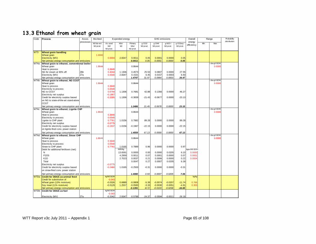
WTT Report v3c July 2011 – Appendix 1 Page 65 of 108
13.3 Ethanol from wheat grain Bio-feed
MJ bio-en/MJ prod.
As usedMJ/
MJ prod.
MJx/MJ
PrimaryMJx/
MJ prod.
g CO2/MJ prod.
g CH4/MJ prod.
g N2O /MJ prod.
g CO2eq /MJ prod.
Min Max
WT3 Wheat grain handlingWheat grain 1.0000Electricity (MV) 0.0004 2.8347 0.0011 0.05 0.0001 0.0000 0.05Net primary energy consumption and emissions 0.0011 0.05 0.0001 0.0000 0.05
WT4a Wheat grain to ethanol, conventional boiler t dw g/t EtOHWheat grain 1.8644 0.8644 3.0300Heat to process 0.3640NG for steam at 90% eff. Z6b 0.4044 1.1306 0.4573 25.53 0.0807 0.0000 27.55Electricity (MV) Z7a 0.0540 2.8347 0.1531 6.45 0.0157 0.0003 6.93Net primary energy consumption and emissions 1.4747 31.97 0.0964 0.0003 34.47
WT4b Wheat grain to ethanol, NG CCGT t dw g/t EtOHWheat grain 1.8644 0.8644 3.0300Heat to process 0.3640Electricity to process 0.0540NG to CCGT 0.6794 1.1306 0.7681 42.88 0.1356 0.0000 46.27Electricity net surplus -0.1867Credit for electricity surplus based on NG to state-of-the-art stand-alone CCGT
-0.3395 1.1306 -0.3839 -21.43 -0.0677 0.0000 -23.13
Net primary energy consumption and emissions 1.2486 21.45 0.0678 0.0000 23.15WT4c Wheat grain to ethanol, Lignite CHP t dw g/t EtOH
Wheat grain 1.8644 0.8644 3.0300Heat to process 0.3640Electricity to process 0.0540Lignite to CHP plant 0.7761 1.0156 0.7882 89.28 0.0000 0.0000 89.28Electricity net surplus -0.0775Credit for electricity surplus based on lignite-fired conv. power station
-0.1937 1.0156 -0.1967 -22.15 0.0000 0.0000 -22.15
Net primary energy consumption and emissions 1.4559 67.13 0.0000 0.0000 67.13WT4d Wheat grain to ethanol, Straw CHP t dw g/t EtOH
Wheat grain 1.8644 0.8644 3.0300Heat to process 0.3640Electricity to process 0.0540Straw to CHP plant 0.7761 1.0165 0.7889 0.96 0.0000 0.0000 0.97Debit for additional fertilisers (net) kWh/kg kgex/MJ EtOH
N 13.6591 0.0000 0.00 0.0000 0.0205 6.10 0.0000 P2O5 4.2959 0.0011 0.07 0.0001 0.0000 0.07 0.0001 K2O 2.7023 0.0037 0.21 0.0006 0.0000 0.22 0.0004 Total 0.0047 0.27 0.0007 0.0205 6.39Electricity net surplus -0.0775Credit for electricity surplus based on straw-fired conv. power station
-0.2460 1.0165 -0.2500 -0.31 0.0000 0.0000 -0.31
Net primary energy consumption and emissions 1.4080 0.93 0.0007 0.0205 7.06WTDa Credit for DDGS as animal feed kg/MJ EtOH kg/kg
Credit for substitution of -0.043Wheat grain (13% moisture) -0.0326 0.6889 -0.0808 -5.39 -0.0074 -0.0207 -11.74 0.766Soy meal (11% moisture) -0.0129 1.2557 -0.0583 -3.33 -0.0030 -0.0051 -4.91 0.303Net primary energy consumption and emissions -0.1391 -8.72 -0.0103 -0.0258 -16.65
WTDb Credit for DDGS as fuel kg/MJ EtOH-0.043
Electricity (MV) Z7a -0.2042 2.8347 -0.5788 -24.37 -0.0594 -0.0011 -26.18
Probability distribution
RangeCode Process Assoc. processes
Expended energy GHG emissions Overall energy
efficiency

WTT Report v3c July 2011 – Appendix 1 Page 66 of 108
WT3 Wheat Grain Handling The data used here are essentially derived from [LowCVP 2004]. On the advice of stakeholders, the drying step in process WT3 has been removed which results in no diesel and lower electricity consumption in this step compared to version 2c of this study. Processes WT4a/b/c/d describe the ethanol plant proper. They all assume the same energy requirement for the plant but different utility generation schemes. WT4a Conventional natural gas boiler Heat is supplied by a conventional natural gas fired boiler and electricity is imported. This can be considered as representative of a number of existing installations and is also by far the cheapest solution. WT4b Combined cycle gas turbine A natural gas fired gas turbine with a heat recovery steam generator (HRSG) provides both heat and electricity. As more heat than electricity is required supplementary firing is applied in the HRSG. As the heat is required only as low pressure steam, a back pressure turbo-generator is also installed behind the HRSG. The plant is assumed to be sized and operated to produce the heat required for ethanol manufacture. There is, however, a surplus of electricity which is exported into the grid, thereby generating an energy and GHG credit. This solution is considerably more energy efficient but also significantly more complex and expensive to build and operate. WT4c Lignite boiler CHP High pressure steam is produced in a lignite boiler. A back pressure turbo-generator produces electricity and low pressure steam for the process. Here again the plant is assumed to be sized and operated to produce the heat required for ethanol manufacture but it nevertheless generates an electricity surplus. After consultation with stakeholders we increased the efficiency of the combined heat and power plant in line with actual plant data resulting in lower energy consumption and emissions compared to version 2c of this study. Lignite (or brown coal) is a cheap and abundant fuel in certain parts of Europe and actual plants are either operating or under construction in Eastern Germany. WT4d Straw boiler CHP Wheat cultivation produces large amounts of straw. Some LCA studies have considered straw as a by-product but this is not necessarily the case. In most of the EU it should be ploughed back to maintain the water-retention properties of the soil (see also straw availability, WTT report, section 5.2.6). Where it may be removed from the field it is partly already used for litter and other applications. Therefore it is misleading to systematically assume that straw can be used to fuel the ethanol production process. In practice this should only be proposed where there is little water stress, a high density of cereals production and a low density of livestock. These conditions would apply to concentrated wheat-producing areas in Northern Europe excluding the Low Countries and Denmark. In any case removing straw will reduce soil nutrients, which needs to be compensated by an additional fertiliser input.

WTT Report v3c July 2011 – Appendix 1 Page 67 of 108
This scheme is similar to the previous case but straw in used instead of lignite. The main advantage of this scheme is to use a renewable source of energy to drive the process. It must be realised, however, that handling and burning of solids is considerably more complex and costly than with liquids or gases, particularly in the case of a low energy density material such as straw. This will therefore be the most expensive option. WTDa Credits for DDGS as animal feed The DDGS credit is calculated according to the methodology referred to in section 13.1. WTDb Credits for DDGS as fuel Although animal feed is by far the most lucrative usage and therefore the most likely, DDGS may also be used as fuel, for instance in solid-burning (i.e. coal) power plants that need to meet their renewable energy obligations. The calorific energy content of DDGS is considerably greater than the energy required to produce the equivalent animal feed, so burning DDGS gives a higher energy credit. WT4e Wheat grain to ethanol, DDGS to biogas So far, use of DDGS has been modelled either as animal feed or as a fuel, directly producing heat and electricity. This new pathway considers an alternative route where the DDGS is fed to a biogas digester. The biogas is fed to a CHP plant providing all the energy required for the plant as well as a surplus of electricity which is exported, thereby generating a credit. We assume that surplus heat cannot be used and so does not generate a credit.

WTT Report v3c July 2011 – Appendix 1 Page 68 of 108
13.4 Ethanol from sugar cane (Brazil)
Bio-feed
MJ bio-en/MJ prod.
As usedMJ/
MJ prod.
MJx/MJ
PrimaryMJx/
MJ prod.
g CO2/MJ prod.
g CH4/MJ prod.
g N2O /MJ prod.
g CO2eq /MJ prod.
Min Max
SC3a Sugar cane to ethanol, heat credit for surplus bagasseSugar cane 2.7720 1.7720Credit for surplus heat (NG) -0.1278 1.1306 -0.1445 -8.0651 -8.7034
kg/MJ EtOH MJ/kgH2SO4 C7 0.00042 4.0052 0.0017 0.08 0.0002 0.0000 0.09CaO C6 0.00047 4.9835 0.0024 0.50 0.0004 0.0000 0.51Cyclohexane 0.00003 9.9000 0.0003 0.00 0.0000 0.0000 0.00Primary energy consumption and emissions 1.6318 -7.48 -0.0249 0.0000 -8.10
SC3b Sugar cane to ethanol, no credit for surplus bagasseSugar cane 2.7720 1.7720
kg/MJ EtOH MJ/kgH2SO4 C7 0.0004 4.0052 0.0017 0.08 0.0002 0.0000 0.09CaO C6 0.0005 4.9835 0.0024 0.50 0.0004 0.0000 0.51Cyclohexane 0.0000 9.9000 0.0003 0.01 0.0000 0.0000 0.01Primary energy consumption and emissions 1.7763 0.59 0.0006 0.0000 0.61
Probability distribution
RangeCode Process Assoc. processes
Expended energy GHG emissions Overall energy
efficiency
SC3a Sugar cane ethanol with credit for surplus bagasse Data for this process were taken from the comprehensive life-cycle analysis by [Macedo 2004], adopting his “scenario 2” which describes best-current-practice in the Centre-South region of Brazil, where 85% Brazilian ethanol is produced. His analysis also takes into account the energy for plant construction and some minor inputs which we neglected to be consistent with our calculations for other processes. The data refer to the production of anhydrous ethanol. Cyclohexane is used in the drying process. The yield corresponds to 91.8 litres ethanol per tonne of moist cane. Inputs were converted from quantities per-tonne-of-cane to per-MJ-ethanol using the same LHV and water content for sugar cane as used in the sugar cane farming process, and standard values for ethanol (see section 1.2). Plant capacity is 120,000 litres ethanol per day, operating for 180 days per year. A very important factor is that the bagasse is used to raise steam which provides all the process heat, and electricity via a steam turbine. In fact modern plants have a surplus of bagasse, usually sold as a fuel for nearby factories (e.g. for food processing), where it mostly replaces fuel oil (almost identical to diesel which we used for credit calculation), and this is what we have modelled. In the future excess bagasse will increasingly be used to generate electricity for export SC3b Sugar cane ethanol, no credit for surplus bagasse This new pathway represents a case where external uses for the surplus bagasse cannot be found. In other aspects it is identical to SC3a. Bagasse is still used to meet the energy needs of the ethanol plant, so overall GHG emissions remain low.

WTT Report v3c July 2011 – Appendix 1 Page 69 of 108
13.5 Biodiesel for plant oil
Bio-feed
MJ bio-en/MJ prod.
As usedMJ/
MJ prod.
MJx/MJ
PrimaryMJx/
MJ prod.
g CO2/MJ prod.
g CH4/MJ prod.
g N2O /MJ prod.
g CO2eq /MJ prod.
Min Max
RO3a Rapeseed to raw oil: extractionRapeseed 1.6326 0.6326 1.5510 1.7142 NormalElectricity (MV) Z7a 0.0092 2.8347 0.0261 1.10 0.0027 0.0000 1.18NG for steam at 90% eff. Z6b 0.0442 1.1306 0.0500 2.79 0.0088 0.0000 3.01 0.0420 0.0464 Normaln-hexane 0.00 0.0031 1.1600 0.0036 0.27 0.0000 0.0000 0.27
kg/MJ prod. MJ/kg
Rapeseed meal (10% moisture) -0.0408Credit for rapeseed meal kg/kg
Soya meal (11% moisture) SYML -0.0156 4.5205 -0.0705 -4.02 -0.0036 -0.0061 -5.94 0.382 Wheat grain (13% moisture) WT1a -0.0195 2.2213 -0.0434 -2.91 -0.0039 -0.0109 -6.24 0.479Primary energy consumption and emissions 0.5983 -2.77 0.0041 -0.0169 -7.71
RO3b Rapeseed to raw oil: extraction, meal to biogasRapeseed 1.6326 0.6326 1.5510 1.7142 NormalElectricity export (MV) Z7a -0.1182 2.8347 -0.3351 -14.11 -0.0344 -0.0006 -15.16Heat surplus (for info, no credit given) 0.0924n-hexane 0.0031 1.1600 0.0036 0.27 0.0000 0.0000 0.27
kg/MJ prod 0.0000Credit for N fertilizer -0.0024 -0.1197 -7.3528 -0.0201 -0.0234 -14.84Primary energy consumption and emissions 0.1815 -21.19 -0.0545 -0.0241 -29.73
SO3a Sunflower seed to raw oil: extractionSunflower seed 1.5200 0.5200 1.4440 1.5960 NormalElectricity (MV) Z7a 0.0085 2.8347 0.0242 1.02 0.0025 0.0000 1.10NG for steam at 90% eff. Z6b 0.0411 1.1306 0.0465 2.59 0.0082 0.0000 2.80 0.0390 0.0431 Normaln-hexane 0.00 0.0029 1.1600 0.0034 0.25 0.0000 0.0000 0.25
kg/MJ prod.
Sunflower seed meal (10% moisture) -0.0361Credit for sunflowerseed meal kg/kg
Soya meal (11% moisture) SYML -0.0088 4.5205 -0.0397 -2.2646 -0.0020 -0.0034 -3.3423 0.215 Wheat grain (13% moisture) WT1a -0.0227 2.2213 -0.0504 -3.3721 -0.0045 -0.0126 -7.2376 0.556Primary energy consumption and emissions 0.5040 -1.77 0.0042 -0.0160 -6.43
SO3b Sunflower seed to raw oil: extraction, meal to biogasSunflower seed 1.5201 0.5201 1.4440 1.5960 NormalElectricity (MV) Z7a 0.0209 2.8347 0.0592 2.49 0.0061 0.0001 2.68NG for steam at 90% eff. Z6b -0.2872 1.1306 -0.3247 -18.13 -0.0573 0.0000 -19.56n-hexane 0.0029 1.1600 0.0034 0.25 0.0000 0.0000 0.25
kg/MJ prod
Credit for N fertilizer -0.0014 -0.0695 -4.2724 -0.0117 -0.0136 -8.62Primary energy consumption and emissions 0.1884 -19.65 -0.0629 -0.0135 -25.25
Probability distribution
RangeCode Process Assoc. processes
Expended energy GHG emissions Overall energy
efficiency
WTT Report v3c July 2011 – Appendix 1 Page 70 of 108
RO3a/b Rapeseed Oil Extraction Rapeseed is crushed and the oil is extracted with the aid of n-hexane solvent and heat. Our data is from [UBA 1999]. [Groves 2002] and [ADEME 2002] have slightly better yield, with slightly higher inputs. The hexane is a refinery product made almost entirely from crude oil: we simplified the other primary energy inputs listed in [FfE 1997] to crude oil equivalents. In all conversion processes, we assume process heat or steam is supplied by a NG boiler working at 90% efficiency. In RO3a the rapeseed cake is used as animal feed, substituting a mix of soy bean and feed wheat according to the generic methodology described in Section 13.1. RO3b is a new process where the rapeseed cake is used to generate biogas which provides all the heat and a large part of the electricity for the process, improving the energy and GHG balance. SO3a/b Sunflower Oil Extraction The process is similar to rapeseed oil extraction with data from [UBA 1999]. The sunflower oil yield is slightly lower than for rapeseed, so more kg of cake are produced per MJ. However, the sunflower seed cake contains less protein (30% dry matter), so the credit for replacing soy beans meal and wheat is smaller.

WTT Report v3c July 2011 – Appendix 1 Page 71 of 108
Bio-feed
MJ bio-en/MJ prod.
As usedMJ/
MJ prod.
MJx/MJ
PrimaryMJx/
MJ prod.
g CO2/MJ prod.
g CH4/MJ prod.
g N2O /MJ prod.
g CO2eq /MJ prod.
Min Max
SY3a Soya beans to raw oil: extraction, meal substituting wheatSoya beans 2.9066 1.9066Electricity (MV) Z7a 0.0343 2.8347 0.0972 4.09 0.0100 0.0002 4.40NG for steam at 90% eff. Z6b 0.1614 1.1306 0.1825 10.19 0.0322 0.0000 11.00 0.1533 0.1696 Squaren-hexane 0.0046 1.1600 0.0053 0.40 0.0000 0.0000 0.40
kg/MJ prod. MJ/kg
Soya meal (11% moisture) -0.118Credit for soya meal kg/kg
Wheat grain (13% moisture) WT1a -0.4581 0.6889 -0.3156 -21.05 -0.0288 -0.0809 -45.86 1.0784Primary energy consumption and emissions 1.8761 -6.36 0.0134 -0.0807 -30.06
SY3b Soya beans to raw oil: extraction, meal substituting corn Soya beans 2.9066 1.9066Electricity (MV) Z7a 0.0343 2.8347 0.0972 4.09 0.0100 0.0002 4.40NG for steam at 90% eff. Z6b 0.1614 1.1306 0.1825 10.19 0.0322 0.0000 11.00 0.1533 0.1696 Squaren-hexane 0.0046 1.1600 0.0053 0.40 0.0000 0.0000 0.40
kg/MJ prod. MJ/kg
Soya meal (11% moisture) -0.118Credit for soya meal kg/kg
Corn CR1 -0.4146 0.6152 -0.2550 -17.57 -0.0166 -0.0624 -36.57 0.976Primary energy consumption and emissions 1.9367 -2.88 0.0256 -0.0622 -20.77
SY3c Soya beans to raw oil: extraction, allocation by market valueSoya beans 1.6869 0.6869Electricity (MV) Z7a 0.0182 2.8347 0.0516 2.17 0.0053 0.0001 2.33NG for steam at 90% eff. Z6b 0.0937 1.1306 0.1059 5.91 0.0187 0.0000 6.38n-hexane 0.0027 1.1600 0.0031 0.23 0.0000 0.0000 0.23Primary energy consumption and emissions 0.8475 8.32 0.0240 0.0001 8.95
Assumptions:- Oil/meal yields: 0.188/0.812- Oil/meal value: 1356/227 $/t- Oil/meal resulting allocation factors: 0.58/0.42
Probability distribution
RangeCode Process Assoc. processes
Expended energy GHG emissions Overall energy
efficiency
SY3a/b Soy beans to raw oil: extraction Soy beans only yield about 20 %m/m of oil, the balance being meal. As a result, when applying a substitution methodology the fate of the meal as a co-product becomes overwhelming in the energy and GHG balance of the oil. Finding a substitute for the meal is difficult since soy bean meal itself is considered the swing source of protein for animal feed. The data for raw oil extraction is taken from [UBA 1999]. In the main WTT report section 3.4.10, we describe how we modified the present “default” SYFA1 pathway scenario. Note that it gives a better GHG balance than that reported in our intermediate posting of results on the internet in November 2008. It uses SY3b process, which assumes that Brazilian soy beans are crushed in EU, and the soy meal by-product substitutes soy meal previously imported from Brazil (unlike the November 2008 scenario, this compensates for the transportation emissions of the soy meal part of the soy beans). Back in Brazil, the reduced price of protein leads to greater inclusion of soy meal in animal diets, at the expense of maize.

WTT Report v3c July 2011 – Appendix 1 Page 72 of 108
Our previous “default” SYFA1 scenario used SY3a for the extraction phase, which grants a credit for soy bean meal produced in EU, replacing EU-wheat. In that case the oil supports the energy burden of transporting the whole beans from Brazil to Europe, so an unfairly poor GHG result was obtained. That pathway is now denoted SYFA1b. For comparison, we also show, SY3c (used in pathway SYFA1c) the result of allocating the soy bean inputs between the oil and the meal on the basis of economic values. Note that the processes as shown do not include the impact of transport for which processes from section 11 are used.
Bio-feed
MJ bio-en/MJ prod.
As usedMJ/
MJ prod.
MJx/MJ
PrimaryMJx/
MJ prod.
g CO2/MJ prod.
g CH4/MJ prod.
g N2O /MJ prod.
g CO2eq /MJ prod.
Min Max
PO3 Palm FFB to raw oil: extractionFFB 1.9000 0.9000
kg/MJ 0.0000 0.0000Palm kernel meal 0.0030Credit for palm kernel meal kg/kg
Soya meal (11% moisture) -0.0048 1.2557 -0.0218 -1.24 -0.0011 -0.0019 -1.83 0.118 Wheat grain (13% moisture) -0.0290 0.6889 -0.0719 -4.79 0.0433 -0.0127 -7.49 0.71Primary energy consumption and emissions 0.8064 -6.04 0.0422 -0.0146 -9.32
PO3a Methane emissions from waste 0.9441 23.60PO3b Credit for surplus heat (diesel) -0.0187 1.1653 -0.0218 -0.27 -0.27
Probability distribution
RangeCode Process Assoc. processes
Expended energy GHG emissions Overall energy
efficiency
PO3 Palm FFB to raw oil: extraction The FFB yields around 20% oil (90% of which is from the flesh, 10% from the kernal). The composition of the two oils is different, but they can both be used to make biofuels. In addition, a small amount of palm kernel meal is produced (about 2.5% of the FFB by mass). This is given credit as animal feed using a mix of soy meal and wheat (See section 13.1). Because there is a large amount of residual biomass, the heat and electricity mill can be powered from this source. Empty fruit bunches are returned to nearby plantations and used as mulch. Methane emissions from waste are assumed to be collected in this process. Figures for yield, heat output from mesocarp fibre and shell palm kernel meal are taken from [Teoh 2004]. PO3a Palm Oil - Methane emissions from waste Waste material from palm oil production can produce significant quantities of methane if stored in anaerobic conditions. There are still differences between the best and worst practices, and even with the best care some emissions from wastewater ponds will occur. We have estimated emissions from wastewater for current best practice using figures from oil industry sources.

WTT Report v3c July 2011 – Appendix 1 Page 73 of 108
PO3b Palm Oil - Credit for surplus heat (diesel) Palm biomass provides sufficient energy to meet the needs of the crushing plant. In addition there is an excess that can be exported to provide local heat where opportunities exist.
Bio-feed
MJ bio-en/MJ prod.
As usedMJ/
MJ prod.
MJx/MJ
PrimaryMJx/
MJ prod.
g CO2/MJ prod.
g CH4/MJ prod.
g N2O /MJ prod.
g CO2eq /MJ prod.
Min Max
RO4 Raw oil to refined oilCrude plant oil 1.0417 0.0417Electricity, MV Z7a 0.0008 2.8347 0.0022 0.09 0.0002 0.0000 0.10NG for steam at 90% eff. Z6b 0.0091 1.1306 0.0103 0.58 0.0018 0.0000 0.62Primary energy consumption and emissions 0.0541 0.67 0.0020 0.0000 0.72
Probability distribution
RangeCode Process Assoc. processes
Expended energy GHG emissions Overall energy
efficiency
RO4 Plant Oil Refining The refining step purifies the plant oil so it is ready for esterification and is assumed to be the same regardless of whether rapeseed, sunflower, soy or palm oil is used. This process, from [UBA 1999], uses, in addition to the fossil energy inputs listed, 6 kg fullers’ earth per t of plant oil for adsorbing impurities. Fullers’ earth is a cheap mineral, with negligible energy input for this quantity. Data are similar to [Groves 2002] and [ADEME 2002].

WTT Report v3c July 2011 – Appendix 1 Page 74 of 108
Bio-feed
MJ bio-en/MJ prod.
As usedMJ/
MJ prod.
MJx/MJ
PrimaryMJx/
MJ prod.
g CO2/MJ prod.
g CH4/MJ prod.
g N2O /MJ prod.
g CO2eq /MJ prod.
Min Max
RO5a Refined oil to FAME: esterificationRefined plant oil 1.0065 0.0065Electricity EU mix, MV Z7a 0.0037 2.8347 0.0106 0.45 0.0011 0.0000 0.48Methanol GA1 0.0585 1.6543 0.0968 5.40 0.0171 0.0000 5.83 0.0556 0.0614NG for steam at 90% eff. Z6b 0.0461 1.1306 0.0521 2.91 0.0092 0.0000 3.14 0.0438 0.0484Various other chemicals 0.00 0.0103 0.14 0.0000 0.0000 0.14Primary energy and emissions(no glycerine credit)
0.1763 8.90 0.0274 0.0000 9.59
kg/MJ prod.
Glycerine -0.00285a Credit for propylene glycol replaced
by glycerineC10 -0.0589 -5.94 -0.0070 -0.0002 -6.16
Primary energy consumption and emissions 0.1173 2.96 0.0204 -0.0001 3.43kg/kg
5b Credit for glycerine replacing wheat grain (LHV basis)
WT1a 1.02 -0.0072 -0.48 -0.0007 -0.0018 -1.04
Primary energy consumption and emissions 0.1691 8.42 0.0267 -0.0018 8.55RO5c Refined oil to FAME: esterification with glycerine to biogas
Refined plant oil 1.0065 0.0065Electricity EU mix, MV Z7a 0.0031 2.8347 0.0087 0.37 0.0009 0.0000 0.39Methanol GA1 0.0585 1.6543 0.0968 5.40 0.02 0.00 5.83 0.0556 0.0614 NormalNG for steam at 90% eff. Z6b 0.0092 1.1306 0.0104 0.58 0.0018 0.0000 0.63 0.0088 0.0097 NormalVarious other chemicals 0.0103 0.14 0.0000 0.0000 0.14Primary energy and emissions 0.1327 6.49 0.0198 0.0000 6.99
RO6a Refined oil to FAEE: esterification Refined plant oil 0.9627 -0.0373Electricity EU mix, MV Z7a 0.0037 2.8347 0.0106 0.45 0.0011 0.0000 0.48Ethanol WTET2a 0.1100 1.4178 0.1560 0.94 0.0026 0.0013 1.40 0.1045 0.1155NG for steam at 90% eff. Z6b 0.0461 1.1306 0.0521 2.91 0.0092 0.0000 3.14 0.0438 0.0484Various other chemicals 0.0030 0.14 0.0000 0.0000 0.14Primary energy and emissions(no glycerine credit)
0.1844 4.43 0.0129 0.0014 5.16
kg/MJ prod.
Glycerine -0.00266a Credit for typical chemical replaced
by glycerineC10 -0.0589 -5.94 -0.0070 -0.0002 -6.16
Primary energy consumption and emissions 0.1254 -1.51 0.0059 0.0012 -1.00kg/kg
6b Credit for glycerine replacing wheat grain (LHV basis)
WT1a 1.02 -0.0003 -0.02 0.0000 0.0000 -0.02
Primary energy consumption and emissions 0.1841 4.41 0.0129 0.0014 5.13Note: in the case of FAEE methanol is replaced by bio-ethanol from pathway WTET2a. The energy used in this process is deemed to remain the sameRO6b Refined oil to FAEE: esterification with glycerine to biogas
Refined plant oil 1.0065 0.0065Electricity EU mix, MV Z7a 0.0031 2.8347 0.0088 0.37 0.0009 0.0000 0.40Ethanol WTET2a 0.1100 1.4178 0.1560 0.94 0.0026 0.0013 1.40 0.1045 0.1155 NormalNG for steam at 90% eff. Z6b 0.0123 1.1306 0.0139 0.78 0.0025 0.0000 0.84Various other chemicals 0.0103 0.14 0.0000 0.0000 0.14Primary energy and emissions 0.1956 2.23 0.0060 0.0014 2.78
Probability distribution
RangeCode Process Assoc. processes
Expended energy GHG emissions Overall energy
efficiency

WTT Report v3c July 2011 – Appendix 1 Page 75 of 108
RO/SO5 Esterification (methanol) The process is the same for rapeseed, sunflower soy and palm oils. Plant oil consists of 3 fatty acid chains on a 3-carbon backbone. 3 molecules of methanol combine with the fatty acids to make 3 molecules of fatty acid methyl ester (FAME), leaving their three alcohol groups stuck on the 3-carbon backbone to form glycerine. 0.1 t methanol reacts with 1 t plant oil to make 0.1 t glycerine and 1 t FAME. Input data are similar to [Groves 2002] and [ADEME 2002]. The LHV of FAME is taken at 37.2 GJ/t, that of glycerine is 16.0 GJ/t [JRC calculation] and methanol is 19.9 GJ/t. Methanol is made mostly from natural gas. “Various other chemicals” aggregates the primary energy inputs and emissions fro a list of minor inputs (NaOH, Na2CO3, H3PO4, HCl) detailed in [UBA 1999] and [GM 2002]. Two credit calculations are made for glycerine. In RO5a/SO5a it is for a typical chemical product; we found data for propylene glycol in [GEMIS 2002], which differs from glycerine only by 1 oxygen atom and is one of many chemicals which glycerine might displace. It uses much less primary energy than synthetic glycerine according to [GM 2002], presumably because the data for the latter includes energy for distilling a pharmaceutical-quality product. Compared to version 2c of this study, the steam requirement for glycerine distillation was corrected downwards and we also removed the glycerine purification step, which was found to be unnecessary. RO5b/SO5b include a credit for glycerine replacing wheat as an animal feed. We know that glycerine is easily digestible by cattle: we assumed that its digestible energy content is 95% of the LHV: the same fraction as for wheat. Then glycerine replaces wheat 1:1 on an LHV basis; we can use our wheat-farming process to calculate the credit. In the new RO5c glycerine is used to produce biogas, significantly reducing the energy input into the process. RO/SO6 Esterification (ethanol) Same as RO/SO5 replacing methanol by ethanol.

WTT Report v3c July 2011 – Appendix 1 Page 76 of 108
13.6 Processes to make materials needed for biomass processing and credit calculations These processes make ingredients for biofuels. As with other biomass processes, we include the LHV and fossil C (as CO2) content of the input fuels in our “MJ primary energy” and CO2 emissions figures associated with fuels inputs.
Code Process Inputkg/
kg prod.As used
MJ/kg prod.
MJx/MJ
PrimaryMJx/
kg prod.
g CO2/kg prod.
g CH4/kg prod.
g N2O/kg prod.
g CO2eq/kg prod.
C6 Pure CaO for processesNatural gas Z6b 4.08 1.1306 4.62 257.7 0.8146 0.0001 278.1Diesel Z1 0.17 1.1600 0.19 16.9 16.9Electricity (EU-mix, MV) Z7a 0.06 2.8347 0.17 7.4 0.0179 0.0003 7.9CaCO3=CaO+CO2 785.7 785.7Primary energy and emissions/kg 4.98 1067.6 0.8326 0.0004 1088.6
C7 Sulphuric acidElectricity (EU mix-MV) Z7a 0.76 2.8347 2.15 90.7 0.2211 0.0041 97.4NG Z6b 1.64 1.1306 1.85 103.4 0.3268 111.6Primary energy and emissions/kg 4.01 194.1 0.5479 0.0041 209.0
C8 AmmoniaNG Z6b 10.90 1.0462 11.40 2323.3 4.3077 2431.0
C10 Propylene glycol (alternative credit for esterification process)Propylene from crude oil 0.0000 6.63 1500.0 1532.8Electricity (EU mix-MV) Z7a 5.00 2.8347 14.17 596.8 1.4554 0.0269 641.2Primary energy and emissions/kg 20.80 2096.8 1.4554 0.0269 2174.0
SY3 Soya meal from crushing beans (same process as for production of soya oil with meal as by-product, now expressed per kg meal)Electricity (EU mix-MV) Z7a 0.29 2.8347 0.82 34.7 0.0846 0.0016 37.3NG for steam at 90% eff. Z6b 1.37 1.1306 1.55 86.4 0.2730 0.0000 93.2n-hexane 0.04 1.1600 0.05 4.0 4.0Plant oil by-product credit (based on sunflower) -0.23 -1.47 -119.5 -0.2684 -0.6211 -311.3Primary energy and emissions/kg 0.94 5.6 0.0892 -0.6195 -176.8
SYML Soya meal supply (for calculation of rape and sunflower meal credit) kg biomass/kg meal
Soy beans farming/kg meal 4.43 0.0927 2.28 154.8 0.1399 1.0125 460.0Soy beans transport/kg meal SY1 4.43 0.0526 1.30 97.8 97.8Soy meal from beans crushing SY2/PO4b 3.60 0.94 5.6 0.0892 -0.6195 -176.8Primary Energy and emissions per kg 4.52 258.1 0.2291 0.3930 381.0
Assoc.processes
Expended energy GHG emissions

WTT Report v3c July 2011 – Appendix 1 Page 77 of 108
C6 Pure CaO for Processes Calcium oxide is used for neutralization in SSCF processes and elsewhere. A more pure grade is required than the lime used in agriculture. Another difference is that the carbon dioxide driven off from limestone in the calcining process is not reabsorbed when the product is used for neutralizing sulphuric acid, for example. So, unlike in lime-for-agriculture, the CO2 emissions from the calcining process should be included. Data is from [GEMIS 2002]. C7 Sulphuric Acid Used in SSCF digestion. Data is from [ESU 1996]. Sulphur mining is neglected. C8 Ammonia Used in SSCF processes. Data is from [Kadam 1999]. C10 Propylene Glycol This is a solvent and antifreeze which could represent the sort of bulk chemical replaced by glycerol from FAME, considering that the extra supply far exceeds the amount of synthetic glycerine still produced The electricity consumption is a preliminary estimate in [GEMIS 2002], and this source also gives primary energies for propylene. Propylene is a refinery product: almost all the input energy is from crude oil, but there are minor credits for gas and coke by-products which we converted to crude-oil equivalents. To convert to MJ, JRC calculated the LHV of propylene; 45.9GJ/tonne, using “HSC for Windows” thermo-chemistry programme. Propylene is a chemical input here, not a fuel being processed. That means we include its LHV and fossil carbon contents (as CO2) in its “primary energy and emissions”. This saves having to add them separately when we come to calculate the credit. SY3 Soy meal from crushing soy beans This is a mass-based process which is needed to calculate the credits per kg of protein-rich animal feeds. The overall process comes from [UBA 1999]. Hexane (solvent used to increase oil recovery) is an oil-refinery product made almost entirely from crude oil. The primary energy inputs listed in [Kaltschmitt 1997] were simplified by converting them to crude oil equivalents. The soy bean oil is treated as a by-product. It attracts an energy and CO2 credit by substituting sunflower oil (in the version 2c of this study we took rapeseed oil as the substitute, but sunflower oil is more similar to soy oil). This is how we calculated the credit: we found the energy and emissions for making 1MJ sunflower oil starting with the energy and emissions from the oil mill (process SO3), and adding (energy and emissions from the sunflower farming, per MJ SFseed)*(MJ of SFseed need to make 1 MJ oil). Then we multiplied all this by the LHV of plant oil (always around 36 MJ/kg) to find the energy and emissions per kg of oil.

WTT Report v3c July 2011 – Appendix 1 Page 78 of 108
Astute readers will have noticed that, since sunflower oil extraction itself has a credit for sunflower meal, which partly replaces soy bean meal, we have a loop. However, this is not a problem: one merely iterates the calculation: the result converges on the correct solution, which can also be attained by elementary algebra. Effectively, a little of the soy oil product needs to be diverted to replace the missing sunflower oil due to the sunflower meal credit: this slightly increases the emissions per MJ of product. SYML Complete soy bean meal production chain Soy bean extraction is the last step in the production chain for soy bean meal. Soy bean farming is included with the farming processes and the transport with the transport processes. Following the scenario in [UBA 1999], the soy beans are imported from the USA and crushed in EU, where the oil replaces rapeseed oil: there is no transport of soy oil. So now we have all the data needed to link the three together to get the total primary energy and emissions from provision of soy meal. The transport calculation has been updated from Version 2. 13.7 Hydrotreated Plant Oil
Bio-feed
MJ bio-en/MJ prod.
As usedMJ/
MJ prod.
MJx/MJ
PrimaryMJx/
MJ prod.
g CO2/MJ prod.
g CH4/MJ prod.
g N2O /MJ prod.
g CO2eq /MJ prod.
Min Max
OY1a Plant oil hydrotreating (NexBTL)Plant oil 1.0341 0.0341Hydrogen (from NG) GH1b 0.0857 1.3150 0.1127 6.20 0.0014 0.0000 6.24 0.0771 0.0943 SquareCredits for energy export NG for steam at 90% eff. Z6b -0.0089 1.1306 -0.0100 -0.56 -0.0018 0.0000 -0.61 Electricity (EU-mix MV) Z7a -0.0017 2.8347 -0.0047 -0.20 -0.0005 0.0000 -0.21Primary energy and emissions 0.1320 5.44 -0.0009 0.0000 5.42
OY1b Plant oil hydrotreating (UOP)Plant oil 0.9100 -0.0900Hydrogen (from NG) GH1b 0.1100 1.3150 0.1447 7.96 0.0018 0.0000 8.01HFO Z3 0.0130 0.0880 0.0011 0.09 0.0000 0.0000 0.09NG for steam at 90% eff. Z6b 0.0144 1.1306 0.0163 0.91 0.0029 0.0000 0.98Electricity (EU-mix MV) Z7a 0.0053 2.8347 0.0149 0.63 0.0015 0.0000 0.67Primary energy and emissions 0.0870 9.59 0.0062 0.0000 9.75
Probability distribution
RangeCode Process Assoc. processes
Expended energy GHG emissions Overall energy
efficiency
We have included two options representing the two processes that are currently on the market i.e. Neste Oil’s NexBTL process and UOP’s Ecofining process. Data were obtained directly from the process licensors in the form of studies carried out on their behalf by consultants. Both processes are similar in purpose although there are differences in implementation.

WTT Report v3c July 2011 – Appendix 1 Page 79 of 108
OY1a Plant Oil Hydrotreating (NexBTL) The data is from [IFEU 2006], a study sponsored by Neste Oil. The process as described produces only diesel i.e. uses the lighter products presumably to produce some of the required hydrogen. OY1b Plant Oil Hydrotreating (UOP) The data is from an unpublished report provided by UOP. The process as described produces diesel as well as small quantities of naphtha and lighter hydrocarbons. In line with what we did for GTL (see section 6.1, process GD1), we allocated the inputs according to the energy content of the products. This results in a higher hydrogen import compared to NexBTL but a lower plant oil consumption.
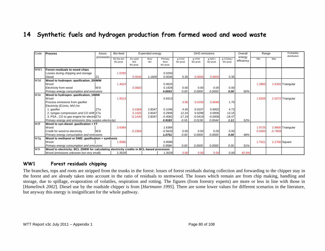
WTT Report v3c July 2011 – Appendix 1 Page 80 of 108
14 Synthetic fuels and hydrogen production from farmed wood and wood waste
Bio-feed
MJ bio-en/MJ prod.
As usedMJ/
MJ prod.
MJx/MJ
PrimaryMJx/
MJ prod.
g CO2/MJ prod.
g CH4/MJ prod.
g N2O /MJ prod.
g CO2eq /MJ prod.
Min Max
WW1 Forest residuals to wood chipsLosses during chipping and storage 1.0250 0.0250Diesel Z1 0.0040 1.1600 0.0046 0.35 0.0000 0.0000 0.35
W3d Wood to hydrogen: gasification, 200MWWood 1.4624 0.4624 1.3893 1.5355 TriangularElectricity from wood W3i 0.0820 0.1929 0.00 0.00 0.00 0.00Primary energy consumption and emissions 0.6553 0.00 0.0000 0.0000 0.00 60%
W3e Wood to hydrogen: gasification, 10MWWood 1.9313 0.9313 1.8339 2.0272 TriangularProcess emissions from gasifier 0.00 0.0150 0.0045 1.70Electricity (EUmix, MV) for 1. gasifier Z7a 0.0369 2.8347 0.1046 4.40 0.0107 0.0002 4.73 2. syngas compression and CO shift Z7a 0.1025 2.8347 0.2906 12.24 0.0298 0.0006 13.15 3. PSA , CO to gas engine for electricZ7a -0.1440 2.8347 -0.4082 -17.19 -0.0419 -0.0008 -18.47Primary energy and emissions (tiny surplus electricity) 0.9183 -0.55 0.0136 0.0044 1.11 52%
W3f Wood to syn-diesel: gasification + FTWood 2.6384 1.6384 1.9725 2.9600 TriangularCredit for wood-to-electricity W3i -0.2394 -0.5633 0.00 0.00 0.00 0.00 0.0000 -0.7859Primary energy consumption and emissions 1.0751 0.00 0.0000 0.0000 0.00 48%
W3g Wood to methanol or DME: gasification + synthesisWood 1.9586 0.9586 1.7021 2.1700 SquarePrimary energy consumption and emissions 0.9586 0.00 0.0000 0.0000 0.00 51%
W3i Wood to electricity: BCL 25MW for calculating electricity credits in BCL-based processes Wood (emissions unknown but very small) 2.3529 1.3529 0.00 0.00 0.00 0.00 42.5%
Code Process Assoc. processes
Expended energy Overall energy
efficiency
Probability distribution
RangeGHG emissions
WW1 Forest residuals chipping The branches, tops and roots are stripped from the trunks in the forest: losses of forest residuals during collection and forwarding to the chipper stay in the forest and are already taken into account in the ratio of residuals to stemwood. The losses which remain are from chip making, handling and storage, due to spillage, evaporation of volatiles, respiration and rotting. The figures (from forestry experts) are more or less in line with those in [Hamelinck 2002]. Diesel use by the roadside chipper is from [Hartmann 1995]. There are some lower values for different scenarios in the literature, but anyway this energy is insignificant for the whole pathway.
WTT Report v3c July 2011 – Appendix 1 Page 81 of 108
14.1 Wood gasification to hydrogen W3d Large scale (200 MW) 200 MW was considered the largest scale of gasifier consistent with economic wood supply from EU-grown forest residuals or farmed wood; it is about the consumption of the largest existing power plant using forest residuals and pulp-mill waste [TEKES 2002]. It is impossible to scale the DM2-type gasifier up to 200MW because of the heat transfer limit through the gasifier walls. For this larger scale, we used a process described in detail by [Katofsky 1993] and [Mann 1997], based on a scale-up of the Batelle-Columbus BCL indirectly-heated circulating fluidized bed gasifier. Sand carries heat to pyrolyse the dried biomass. The cooled sand and coke left from the pyrolysis returns to a separate combustion section, where it is burnt in air. In this way the syngas from the pyrolysis section is not diluted with nitrogen. The syngas goes through conventional cold (wet) gas-cleaning and is then compressed into a 950°C reformer, to convert hydrocarbons to CO and H2, followed by a 2-stage shift reactor to adjust the H2/CO ratio. Hydrogen is separated by PSA and the remaining CO is burnt in a combined cycle electricity power-plant. However, the process is so optimised for hydrogen production that the electricity generated by the waste gas in the power plant is not sufficient to cover all the needs of the plant. If we were to give a debit for provision of grid electricity, GHG emissions and fossil energy use would appear on the bottom line. This would give an unfair impression when comparing with other processes which maybe produce much less fuel but a little more electricity. Effectively these other processes have improved their energy/GHG per MJ fuel by incorporating part of a wood-to-electricity process. To even things up, we made all processes electricity-neutral by giving electricity credits or debits using the nearest equivalent wood-to-electricity process. In the case of W3d, we chose a wood-to-electricity pathway from the literature which uses the same gasifier (BCL). It is shown at the bottom of the table as W3i. The overall result is about the same as the [Katofsky 1993] process de-optimized to give a little more electricity and a little less hydrogen. In doing this, we have not departed from our principle of subtracting a “reference scenario” from a “biofuels” scenario. The nature of the process forces us to produce both hydrogen and bio-electricity in the biofuel scenario: to find the contribution only of the hydrogen production, we should produce the same quantity of bio-electricity in the reference scenario. This is the same as a bio-electricity credit. W3e Small scale (10MW) This is a process intended for hydrogen production from local wood resources. It was calculated by LBST, based on the CHOREN DM2 10 MWth externally-heated gasifier [Schmid 2001]. The moist wood is pyrolysed (with a simultaneous reforming reaction) using heat from the coke by-product. It can cope with wood with up to 35% moisture, but the process efficiency is calculated for 30% moisture in the wood, when the cold gas efficiency of the gasifier is 76.4% [Schmid 2001]. The syngas is compressed into a catalytic shift reactor to increase the hydrogen content up to about 66% at the expense of CO. The hydrogen is separated in a Pressure-Swing-Adsorption (PSA) system. The rest of the syngas is burnt for process power and heat in a micro turbine with 24% electrical efficiency and 51% process heat recovery. The process is very nearly electricity-neutral.

WTT Report v3c July 2011 – Appendix 1 Page 82 of 108
14.2 Synthetic fuels from wood gasification W3f Synthetic Diesel from Wood Our “best estimate” is based on the study by [Tijmensen 2002]. In the variant we chose, syngas from the BCL gasifier (the same as in the 200 MWth hydrogen process) passes cold gas cleaning, a reformer and shift-reactor as in the hydrogen process. An amine process removes the CO2 and the rest of the syngas enters a fixed-bed Fischer-Tropsch reactor, which builds alkanes from reacting CO and hydrogen on the surface of the catalyst. The reaction conditions are adjusted to maximize the direct production of liquids (gasoil, kerosene and naphtha), which are condensed from the off-gas. Co-products are unreacted gas, LPG vapour and wax. The wax is hydrocracked to make more diesel and naphtha. In our chosen variant, which maximizes diesel yield, up to 2/3 of the unreacted gas (+LPG) is recycled to pass the FT reactor again. The LPG in the recycle does not react: once the alkyl chain is terminated, it cannot be re-opened by the FT catalyst. The off-gas that is not recycled in our variant is burnt in a condensing combined cycle for process heat and electricity. This produces an excess of electricity, for which we give a wood credit, using process W3i: electricity from BCL gasifier. This simulates an electricity-neutral process as explained above. The process yield, efficiency and the product mix depends on the performance of the FT catalyst, which determines the chain growth probability (CGP). [Tijmensen 2002] took a range of likely CGP values, because the catalyst performance is difficult to predict. We took their average CGP (0.85) for our best-estimate case. The composition of the FT liquids condensed after the reactor has to be found from figure 2 of [Tijmensen 2002]: about 35% m/m naphtha and 65% m/m middle distillates (= gasoil + kerosene). To this should be added the products of wax cracking. The mass of wax produced is 19% of the FT liquids, and if cracked so as to maximize gasoil, yields 15% of its mass in naphtha and 85% diesel. Bearing in mind also that naphtha has slightly higher LHV than diesel (44.5 vs. 44.0 MJ/kg) the overall product mix turns out to be 68% diesel and 32% naphtha in energy terms. For our worst-case we took the lowest CGP (0.8) considered by [Tijmensen 2002]. Then we calculated the overall product mix is 57% diesel and 43% naphtha in LHV terms. There is a wood credit for electricity as before. For our best case, no variant in [Tijmensen 2002] can match the yield and efficiency (51%) claimed by [CHOREN 2003] for a projected biogas-to-liquids process based on the DMT gasifier. The CHOREN process is electrically neutral. They project 100% diesel product. That means all the non-diesel components, which are an inevitable product of the FT reaction, have to be fed back to the gasifier (the FT reactor cannot grow chains which are already terminated). For calculations using W3f we chose a triangular probability distribution drawn between the three cases. W3g Wood to methanol or DME DME can be thought of as dehydrated methanol: the only difference between the synthesis processes is in the final catalyst reactor so that the efficiencies are more or less the same.

WTT Report v3c July 2011 – Appendix 1 Page 83 of 108
Our “best-case” process is based on [Katofsky 1993], using the BCL indirectly-heated gasifier with wet gas cleaning and reforming of higher hydrocarbons. The rest of the process is similar to methanol synthesis from natural gas. A conventional, fixed bed methanol reactor is used. With all fuel synthesis routes, it might be possible to improve efficiency by using slurry reactors or hot gas cleaning. However, neither has been demonstrated for synthesis from bio-syngas: there are question marks about gas quality [Tijmensen 2002]. Furthermore, the use of conventional processes enables us to compare all routes on a fair basis. Our “worst case” is based on oxygen-blowing the Värnamo autothermal pressurized fluidized bed gasifier, modelled by [Atrax 1999]. Although this is a state-of-the art gasifier, it is not as sophisticated and expensive as the BCL gasifier. The process uses the hot gas filtration demonstrated at Värnamo to allow the gas to go hot into the 950°C steam reformer, where some tar is also decomposed. However, after the shift water-gas shift reactor (to boost the H2/CO ratio), it is still necessary to use a scrubbing process to remove impurities (including HCl, H2S…) before the gas is pure enough for synthesis. In the Altrax process the purification is combined with CO2 removal by scrubbing with methanol (Rectisol Process). The DME synthesis process (by Haldor Topsoe A/S) is similar to that in the 200 MW plant. The efficiency is lower than the BCL-gasifier process because of the energy consumption by the oxygen separation plant, and because the H2/CO ratio in the raw syngas is lower. Again we assume that methanol could be produced at the same efficiency as DME.

WTT Report v3c July 2011 – Appendix 1 Page 84 of 108
14.3 Ethanol from cellulosic biomass (farmed wood, wood waste and straw)
Bio-feed
MJ bio-en/MJ prod.
As usedMJ/
MJ prod.
MJx/MJ
PrimaryMJx/
MJ prod.
g CO2/MJ prod.
g CH4/MJ prod.
g N2O /MJ prod.
g CO2eq /MJ prod.
Min Max
W3j Woody biomass to ethanol (SSCF) kgex/
Biomass input 2.9170 1.9170 MJprod. 2.7550 3.0790 SquareCredit for wood-to-electricity W3a -0.0995 3.125 -0.3108 0.00 -0.0026 -0.0002 -0.14Diesel Z1 0.0358 1.160 0.0415 3.13 0.0000 0.0000 3.13H2SO4 C7 1.113 0.0142 0.69 0.0019 0.0000 0.74 0.0035NH3 C8 12.324 0.1205 6.31 0.0117 0.0000 6.61 0.0027(NH4)2SO4 C7,C8 3.983 0.0107 0.55 0.0011 0.0000 0.58 0.0007Antifoam 5.778 0.0090 0.90 0.0011 0.0000 0.94 0.0004Corn Steep Liquor 0.000 0.0000 0.00 0.0000 0.0000 0.00 0.0038CaO C6 1.384 0.0068 1.45 0.0011 0.0000 1.48 0.0014Primary energy consumption and emissions 1.8089 13.03 0.0144 -0.0002 13.33 36%
W3k Wheat straw to ethanol (Iogen)Straw 2.3770 1.3770 0.4891Transport of straw WT2b 0.0089 0.22 0.0000 0.0000 0.22Credit for straw-to-electricity W3a -0.0520 3.125 -0.1651 0.00 -0.0014 -0.0001 -0.07H2SO4 C7 1.113 0.0167 0.81 0.0023 0.0000 0.87 0.0042NH3 C8 0.000 0.0000 0.00 0.0000 0.0000 0.00 0.0000(NH4)2SO4 C7,C8 0.000 0.0000 0.00 0.0000 0.0000 0.00 0.0000Antifoam 0.000 0.0000 0.00 0.0000 0.0000 0.00 0.0000Corn Steep Liquor 0.000 0.0000 0.00 0.0000 0.0000 0.00 0.0000CaO C6 1.384 0.0119 2.54 0.0020 0.0000 2.59 0.0024Debit for additional fertilisers N 13.6591 0.0000 0.00 0.00 0.00 0.00 0.0000 P 4.2959 0.0049 0.31 0.00 0.00 0.32 0.0003 K 2.7023 0.0164 0.92 0.00 0.00 0.99 0.0017
0.0213 1.23 0.0030 0.0000 1.31Primary energy consumption and emissions 1.2707 4.80 0.0059 -0.0001 4.92 44%
Code Process Assoc. processes
Expended energy Overall energy
efficiency
Probability distribution
RangeGHG emissions

WTT Report v3c July 2011 – Appendix 1 Page 85 of 108
W3j Ethanol from woody biomass; worst/best case This corresponds to the “base case” of the detailed study by NERL [Wooley 1999] on wood-to-ethanol via SSCF (Simultaneous Saccharification and Co-Fermentation). The base case combined the best equipment and processes which were had been demonstrated in 1999. Our “best case” is the ”best of industry” case in [Wooley 1999], which incorporates the technical advances which could be foreseen to flow from laboratory developments known in 1999. It was not considered that NREL’s more futuristic projections fitted in the time-frame of this study. Wood consists principally of hemicellulose, cellulose and lignin. Wood chips are ground, steamed and then hydrolysed in dilute sulphuric acid to release the sugars from the hemicellulose. The product is neutralised and detoxified, and part goes to breed enzyme-producing aerobic bacteria with the aid of additional nutrients (such as corn steep liquor). The bacteria-rich stream then joins the main stream in the main fermentor, where enzymatic breakdown of cellulose (saccharification) occurs simultaneously with fermentation of the different sugars released. After several days, the “beer” is sent for distillation. The slops (including lignin) are dried and burnt to raise steam, along with biogas from the waste water treatment. Surplus steam goes to turbine to make electricity. The NREL process has an excess of electricity. Like the other wood conversion processes, our process is made electricity-neutral by giving a wood credit for the electricity produced. Since this is not a gasifier-based process, we calculated the credit using a conventional wood-fired steam turbine condensing power station, based on LBST data from the plant at Altenstadt, Germany (see wood-to-electricity processes).. The processes to make the input chemicals are described above (section 1.10: chemicals), with two exceptions, for which we could find no quantitative data: corn steep liquor (CSL) and antifoam. CSL is a by-product from corn syrup manufacture, used as a culture medium for bacteria, and as animal feed. Usually it is neglected in LCA studies. To check if it could be significant, we gave it a (MJ primary energy input)/ (MJ digestible energy) ratio the same as wheat. This confirmed that it could have been neglected. Antifoam is a simple silicone compound. Instead of neglecting it a priori we attributed a primary energy per kg typical of a process chemical, which showed it to be of no unimportant in the energy balance. W3k Ethanol from straw Data for a 150 MW straw-to-ethanol SSCF plant was supplied to the study by Iogen corp., who operate a commercial plant for straw to ethanol in Iowa [Iogen 2003]. A biomass credit is given for electricity export again based on the Altenstadt wood-burning power station (the straw-burning power plant at Sanguesa in Spain has a similar efficiency). Of the chemicals inputs, Iogen only specified sulphuric acid consumption, which is lower than for the wood-to-ethanol process because of a more favourable composition. We assumed that the other chemicals (e.g. for neutralization) mentioned by [Wooley 1999] are also needed by the straw process, in proportion to the lower sulphuric acid requirements. The yield calculation applied to wood gives about the wood-to-ethanol yields claimed in [Wooley 1999]. Furthermore, we used the same procedure for the straw-to-SSCF part of process, and came up with energy and emissions figures almost the same as for a commercial state-of-the art straw-to-ethanol process.

WTT Report v3c July 2011 – Appendix 1 Page 86 of 108
The distillation steps and possibly fermentation steps could be combined with the main process: however, for the sake of energy calculation the processes are kept separate. The first paragraph shows that to get 1 MJ ethanol from the combined process we need we need 0.198/(1+0.198) = 0.165 MJ from our new pulp-to SSCF process (without pulp credits), and 0.835 MJ from the conventional sugar-beet process. 14.4 Synthetic fuels and hydrogen from waste wood via Black Liquor
Bio-feed
MJ bio-en/MJ prod.
As usedMJ/
MJ prod.
MJx/MJ
PrimaryMJx/
MJ prod.
g CO2/MJ prod.
g CH4/MJ prod.
g N2O /MJ prod.
g CO2eq /MJ prod.
Min Max
BLH Wood waste to hydrogen via black liquorWood waste 1.2410 0.2410 1.1790 1.3031 SquarePrimary energy consumption and emissions 0.2410 0.00 0.0000 0.0000 0.00 81%
BLD Wood waste to DME via black liquorWood waste 1.4851 0.4851 1.4108 1.5594 SquarePrimary energy consumption and emissions 0.4851 0.00 0.0000 0.0000 0.00 67%
BLM Wood waste to methanol via black liquorWood waste 1.5180 0.5180 1.4421 1.5939 SquarePrimary energy consumption and emissions 0.5180 0.00 0.0000 0.0000 0.00 66%
BLS Wood waste to syn diesel via black liquorWood waste 1.8280 0.8280 1.7366 1.9194 SquarePrimary energy consumption and emissions 0.8280 0.00 0.0000 0.0000 0.00 55%
Code Process Assoc. processes
Expended energy Overall energy
efficiency
Probability distribution
RangeGHG emissions
BLD/M Wood waste to DME/Methanol Black liquor is the residue of the paper pulp making process. It is a water-based slurry, 70 to 80% of which consists of lignin and spent pulping chemicals. In conventional pulp mills it is burned in a so-called "recovery boiler" to provide process heat; boiler efficiency is limited to about 65% because of the corrosive nature of the molten salts present (mostly Na2S and Na2CO3). With the addition of steam from a “hog boiler” burning bark and other wood waste produced on site, a modern pulp mill is self-sufficient in heat, and can even export some electricity. Alternatively the organic portion of the black liquor can be converted into syngas is an oxygen-blown gasifier. An air separation unit is needed. The syngas can then be either burnt to produce electricity or converted into hydrogen, methanol, DME or hydrocarbons. As part of the energy content of the black liquor ends up in the fuel, additional heat is needed for the pulping process. This is provided by increasing the amount of biomass fed to the hog boiler. The cheapest source of extra biomass is forest residuals (branches, tops, undersize trees and occasionally roots), which can be collected at the time of felling and brought to the pulp mill using the same transport infrastructure as the stem-wood. Taking the original pulp mill as reference, and adjusting the new process to give the same pulp production and electricity balance, one can calculate the extra wood residuals required to produce a given amount of fuel product. This effective efficiency turns out to be appreciably higher than that of a stand-alone gasifier conversion process. The reason is that the additional burning of forest residuals increases the thermal capacity of the plant, whilst
WTT Report v3c July 2011 – Appendix 1 Page 87 of 108
the stack losses are reduced because the hog-fuel boiler has higher efficiency than the replaced recovery boiler. Almost all the heat from the syngas is recovered. Our data are from the thorough technical and commercial feasibility study of methanol and DME production via black liquor gasification carried out for DG-TREN’s ALTENER programme [Ekbom 2003]. The study first modelled a modern reference pulp mill (“KAM2” model mill), recycling all wood wastes produced in the mill, but not importing residuals from the forest. This is self-sufficient in heat, and produces a small electricity surplus from a condensing steam turbine generator. Production capacity is 2000 dry tonnes pulp per day. Then [Ekbom 2003] modelled the BLGMF (“Black Liquor Gasifier for Motor Fuels”) plant to be also self-sufficient on heat and with the same pulp production and electricity export. The electricity is produced by a condensing steam turbine, even though higher efficiencies could be obtained from an advanced combined cycle generator incorporating a gas turbine. The difference between the BLGMF model and the KAM2 reference mill showed that 272.8 MW methanol would be produced with an additional biomass consumption of 414.1 MW biomass. Thus 1 MJ methanol requires 1.518 MJ biomass and the energy conversion efficiency is 65.9%. For the process producing DME, which differs from the methanol process only in the catalyst and conditions in the final synthesis stage, 275 MW DME are produced from 408 MW biomass, so 1 MJ methanol requires 1.485 MJ biomass, a conversion efficiency of 71%. We added a ±5% error range to these figures. [Ekbom 2003] also provides estimates of the incremental plant investment, assuming that the recovery boiler in the pulp mill was anyway due for replacement. We used their estimates of 150.3 M€ for the methanol plant and 164.2 M€ for the DME plant in our costing calculations.

WTT Report v3c July 2011 – Appendix 1 Page 88 of 108
Fig. 14.4 Schematic process flow diagram of the BLGMF-methanol plant, reproduced with permission from [Ekbom 2003]
BLS Wood waste to FT via black liquor gasification We estimated the efficiency of this route by replacing the methanol synthesis in [Ekbom 2003] with the FT process described in [Shell 1990]. The process uses stream 11 in Figure 14.4. The FT process consists of an FT synthesis step in which hydrocarbons are grown on catalysts by the reaction of CO and hydrogen. To get a high diesel yield and little unreacted gas, FT synthesis is allowed to continue to produce heavy hydrocarbons, which are then cracked downstream in a hydrogen cracker. Nevertheless, a distribution of hydrocarbons is produced. [Shell 1990] does not specify the distribution of <C10, so this had to model it from chain growth statistics, in order to calculate the energy balance. The Shell process yields about 77 % m/m C10-C20 products (diesel+kerosene; usable in diesel engines) and 23% naphtha on either energy or mass basis. Compared to the reference pulp

WTT Report v3c July 2011 – Appendix 1 Page 89 of 108
mill, the whole BGLF-FT process produces 194 MW C10-C20 hydrocarbons and 59.1 MW naphtha from 414 MW extra biomass. Thus 1 MJ extra biomass would produce a total of 0.47 MJ of kerosene/diesel mixture together with 0.14 MJ naphtha (<C9). If one wishes to produce only diesel and kerosene (to compare with the claims for the Choren wood-FT process, for example), the other products must be recycled. We assumed that the naphtha is added to the hog boiler to produce electricity. To keep the electricity generation the same as the reference pulp plant, we should remove the same MJ of biomass. Therefore only 0.86 MJ biomass are needed to make 0.47 MJ kerosene/diesel by itself. Thus the efficiency to kerosene/diesel is 55% and 1.83 MJ biomass are needed to make 1 MJ kerosene/diesel. Before this report was finalized, [Ekbom 2005] produced their own, more detailed, calculation of FT-diesel efficiency using BLGMF process, incorporating product fractionation. It is difficult to compare our model with theirs, because they calculated product mixtures from fractionation rather than simply assigning carbon numbers. Their results indicate that each 1MJ extra biomass would produce 0.43 MJ diesel-quality distillate together with 0.22 MJ naphtha. If we perform the same credit for recycling the naphtha as for our calculation above, we deduce that an extra 0.78 MJ biomass in the pulp mill would give 0.43 MJ diesel-quality distillate. That corresponds to an efficiency to diesel fuel of 55%: exactly the same as in our own calculation. Such close agreement may be fortuitous, but it was comforting to have independent confirmation. We estimated that the incremental cost of installing a BLGMF-FT plant in a pulp mill which needs a new recovery boiler would be about 260 M€ ±20%. Subsequently, [Ekbom 2005] estimated the figure to be 205 M€. Considering that this is the cost of the new plant minus 171 M€, representing the saved cost of a new recovery boiler, the difference between the two estimates of the cost of a BLGMF-FT plant is only 13%. BLH Wood waste to hydrogen via black liquor gasification Neither [Ekbom 2003] nor [Ekbom 2005] considered this process. We took their detailed description of the BLGMF plant and considered what modifications would be needed to make hydrogen instead of methanol. The methanol synthesis and distillation are not needed, but a larger CO shift reactor is required, coupled to a pressure swing absorption (PSA) to purify the hydrogen. The hydrogen process starts from stream 4 in Figure 14.4. All this goes to the CO-shift instead of only half for the methanol plant. Therefore more steam is required for the CO shift reactor, but on the other hand the outlet of the CO shift contains more steam, because more is formed in the reaction. The net amount of steam compared with the methanol plant depends on whether the shift reaction is exothermic or endothermic. If we calculate this starting from steam, it is slightly exothermic, but if we include the energy for generating the steam from water, it is slightly endothermic. In practice, one could find a source of steam, but a little less heat would be recovered. Thus the difference in steam requirements is approximately zero. The CO2 absorption (Abs 2) is not required because CO2 is anyway removed downstream in the PSA. The pressure at the outlet of the CO shift reactor (2.9 MPa; [Ekbom 2003]) is sufficient to drive the PSA process. Hydrogen recovery is assumed to be 86%; the tail-gases can be burnt for steam and electricity.

WTT Report v3c July 2011 – Appendix 1 Page 90 of 108
Compared to the reference pulp mill, the BGLF-hydrogen process produces 247 MW H2 and 108.3 MW of the other gases. Thus 1MJ extra biomass would produce 0.594 MJ hydrogen and leave 0.261 MJ in the tail-gas. If the tail gas is added to the boiler of the existing condensing steam-turbine generator, it will save the same energy input of biomass. Therefore only 0.839 MJ biomass are needed to 0.594 MJ hydrogen by itself. Thus the efficiency to hydrogen is 81% and 1.24 MJ biomass are needed to make 1 MJ hydrogen. In [Katofsky 1993], the cost of a hydrogen plant based on the BCL wood gasifier is 27 M€ less than that of a methanol plant based on the same gasifier. The hydrogen and methanol synthesis processes are similar to the ones described here, and have roughly the same scale. Since the BLGMF-methanol plant costs 150.3 M€ in [Ekbom 2003] (taking into account the saving on a new recovery boiler), we expect a BLGMF hydrogen plant would cost 123 M€ on the same basis.

WTT Report v3c July 2011 – Appendix 1 Page 91 of 108
15 Heat and Electricity (co)Generation 15.1 Electricity only
Code Process Expended
energyMJx/MJe
g CO2/MJe
g CH4/MJe
g N2O/MJe
g CO2eq/MJe
Min Max
GE Electricity from NG (CCGT)KE1 Electricity from Coal (conv. Boiler)
Energy as hard coal 1.3000 221.45 221.45 43.5% 1.0000 1.5000 Dble triKE2 Electricity from Coal (IGCC)
Energy as hard coal 1.0833 200.58 200.58 48.0% 0.9231 1.2435 EqualKE2C Electricity from Coal (IGCC) + CO2 capture
Energy as hard coal 1.4390 23.44 23.44 41.0% 1.2680 1.6100 EqualW3a Electricity from wood steam boiler
Energy as wood 2.1250 0.0828 0.0247 9.44 32.0% 1.9688 2.2813 NormalW3b Electricity from 200 MWth wood gasifier
Energy as wood 1.0747 0.0262 1.40 48.2% 1.0000 1.1739 NormalW3c Electricity from 10 MWth wood gasifier
Energy as wood 1.8228 0.0356 1.90 35.4% 1.6817 1.9639 NormalBLE Electricity from waste wood via black liquor
Waste wood 0.1111 0.00 0.0000 0.0000 0.00 90.0% 0.0555 0.1667 EqualW3h Wood cofiring in coal-fired power station
Wood 1.3000 0.00 0.0041 0.0114 3.49 43.5% 1.0000 1.5000 Double triangleDE Electricity from wind
Energy as wind 0.0000NE1 Nuclear fuel provision
Nuclear 0.1805 0.0%NG 0.0045Crude oil 0.0025Waste 0.0018Hard coal 0.0053Brown coalHydropower 0.0012Total 0.1977 1.21 0.0029 0.0001 1.30
NE2 Electricity from nuclearEnergy as diesel 0.0000 0.07Energy as uranium 2.0303 33.0%
RangeGHG emissions Eff Probability distribution

WTT Report v3c July 2011 – Appendix 1 Page 92 of 108
GE Electricity from NG This process represents the now standard route for efficient and cost-effective production of electric power from gas i.e. a combined cycle gas turbine complex. The overall efficiency of 55% is typical of modern state-of-the-art plants, the ± 5% range representing the range of existing and foreseeable technologies [GEMIS 2002], [TAB 1999] (see also section 5.1, process GG2). KE1 Electricity from coal (conv. boiler) This state-of-the-art conventional route is assumed to have a typical efficiency of 43.5%. KE2 Electricity from coal (IGCC) The IGCC (integrated gasification and combined cycle) alternative reaches an efficiency of 50% [TAB 1999]. For electricity from wood, 4 alternatives are considered, i.e. via a steam boiler plus turbine plant (W3a), wood gasification at either large or small scale (W3b/c) and finally indirectly via gasification of black liquor in a paper mill. All incorporate drying of fuel using heat from the flue gas. Forest residuals chipping is the same process as in the wood-to-hydrogen and synthetic fuels process table above. It includes dry matter losses during storage and ex-forest handling. For farmed wood, chipping is included in the farming process. W3a Electricity from wood steam boiler The small conventional plant is based on LBST data for the 11.5 MW fluidized-bed condensing steam-turbine power plant at Altenstadt, Germany. Fluidized bed combustors cope better with the varying quality of fuel from wood chips than conventional grate boilers. W3b Electricity from 200 MWth wood gasifier The large gasifier power station is taken from the study by [Sydcraft 2001] of an IGCC based on the Värnamo pressurized fluidized bed gasifier, using a state-of-the-art GTX 100 gas turbine with flue gas condensation (140 MWth). This configuration maximizes the electrical efficiency. The lower efficiency limit is for the existing turbine at Värnamo, whilst the upper limit projects a further 2% in gas turbine efficiency by 2010. We selected this power station because the Värnamo gasifier is the only one which has been demonstrated to work with hot gas filtration, which gives a significant improvement in efficiency since the syngas enters hot into the turbine, and will surely become the norm for future IGCC power stations. W3c Electricity from 10 MWth wood gasifier Data are from the Oeko-Institut’s EM generic database, which also supplies cost data. We consider 5% uncertainty in the LHV efficiency. Gasifiers give higher electrical efficiency and can cope with varying fuel quality. But the investment cost is higher: not worth it if one can use the waste heat for district heating.

WTT Report v3c July 2011 – Appendix 1 Page 93 of 108
BLE Electricity from waste wood via black liquor Instead of using the output of the gasifier in a BLGMF plant for motor-fuel synthesis (section 14.4), one can burn the syngas for electricity cogeneration. Again, the heat balance of the plant is restored by burning additional biomass in the hog boiler. In the same way that [Ekbom 2003] analysed fuel-producing BLGMF [Berglin 1999] analysed different options for electricity production by replacing the black liquor recovery boiler with an oxygen-blown gasifier. The efficiency of electricity production is found by dividing the increased electricity production by the increased biomass consumption, compared to the reference mill. A little confusingly, [Berglin 1999] adopts a modern integrated pulp/paper mill as the reference mill, instead of the modern pulp-only-mill in [Ekbom 2003]. However, the changes are all in the pulp section, this should not affect the results (Berglin does this to demonstrate that the extra electricity produced could be sufficient to make the whole paper mill self-sufficient on energy, instead of consuming electricity, as at present). The syngas is cleaned, and burnt in a combined cycle of back-pressure steam turbine, condensing steam turbine and gas turbine. Berglin discusses many different options, including three ways to remove the H2S from the syngas. We chose the variant (“case 6”, table 7 in [Berglin 1999]) which produces the highest electricity export, though not at the highest incremental efficiency. It removes H2S from the syngas by reabsorbing it in the white liquor. That means it uses more lime, but the lime is regenerated in a closed cycle as part of the system, so the energy implications are fully taken into account. The gas turbine assumed in this variant has an input temperature of 1430ºC, with a pressure ratio 20, and the maximum steam temperature is 530ºC. The gasifier operates at 37 bar. The plant produces electricity from biomass (bark or forest residuals) at an incremental efficiency of 90%, because it benefits from the reduction in stack losses and increased thermal capacity in the paper mill. W3h Wood co-firing in coal-fired power station Wood energy is assumed to be converted to electricity with the same efficiency as the generic KE1 coal process above. DE Electricity from wind Contrary to biomass, wind energy is in effect inexhaustible, the limitation being in the equipment used to harness it. The notion of efficiency becomes therefore academic in this case. We have shown it as 100% efficient. The energy associated with operation and maintenance is very small. NE1 Nuclear fuel provision The figures used are typical of the European supply of nuclear fuel [GEMIS 2002]. NE2 Electricity from nuclear The figures used here pertain to conventional nuclear reactors turning the nuclear reaction heat into steam feeding turbines. The efficiency figure is the fraction of the heat released by the nuclear reaction and transferred to the steam that is turned into electricity [GEMIS 2002].
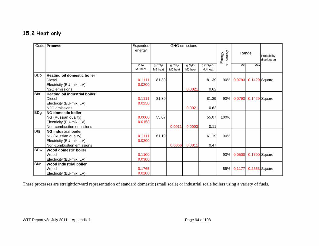
WTT Report v3c July 2011 – Appendix 1 Page 94 of 108
15.2 Heat only
Code Process Expended energy
MJx/MJ heat
g CO2/MJ heat
g CH4/MJ heat
g N2O/MJ heat
g CO2eq/MJ heat
Min Max
BDo Heating oil domestic boilerDiesel 0.1111 81.39 81.39 90% 0.0793 0.1429 SquareElectricity (EU-mix, LV) 0.0200N2O emissions 0.0021 0.62
BIo Heating oil industrial boilerDiesel 0.1111 81.39 81.39 90% 0.0793 0.1429 SquareElectricity (EU-mix, LV) 0.0250N2O emissions 0.0021 0.62
BDg NG domestic boilerNG (Russian quality) 0.0000 55.07 55.07 100%Electricity (EU-mix, LV) 0.0158Non-combustion emissions 0.0011 0.0003 0.11
BIg NG industrial boilerNG (Russian quality) 0.1111 61.19 61.19 90%Electricity (EU-mix, LV) 0.0200Non-combustion emissions 0.0056 0.0011 0.47
BDw Wood domestic boilerWood 0.1100 90% 0.0500 0.1700 SquareElectricity (EU-mix, LV) 0.0300
BIw Wood industrial boilerWood 0.1765 85% 0.1177 0.2353 SquareElectricity (EU-mix, LV) 0.0200
RangeProbability distribution
GHG emissions
Ener
gyef
ficie
ncy
These processes are straightforward representation of standard domestic (small scale) or industrial scale boilers using a variety of fuels.

WTT Report v3c July 2011 – Appendix 1 Page 95 of 108
15.3 Combined Heat and Power (CHP)
Code Process Total energy
MJ g CO2 g CH4 g N2O g CO2eq Min Max
The energy figures are shown in total energy input to produce one unit of heat+power. Only direct emissions from the boilers are shownHPg CHP plant, gas fired
NG (Russian quality) 2.3280 128.21 128.21 90% 2.2220 2.4340 SquareElectricity (HV) -1.0000Heat -1.0950Non-combustion emissions 0.0097 0.0056 1.90
HPw CHP plant, wood firedWood 4.4500 0.00 0.00 79% 4.2300 4.6700 SquareElectricity (HV) -1.0000Heat -2.5000Non-combustion emissions 0.0922 0.0028 3.13
GHG emissions
Ener
gyef
ficie
ncy
RangeProbability distribution
In this case the energy input shown if the total energy relating to 1 MJ of electricity produced. Usable heat is produced at the same time resulting in a very high total efficiency (defined as the sum of the energy content of the heat + electricity divided by the heat content of the feedstock). In the corresponding full pathways the figures are shown as energy expanded per MJ of electricity produced, with a credit calculated for the heat (see WTT Appendix 2).

WTT Report v3c July 2011 – Appendix 1 Page 96 of 108
16 Hydrogen from electrolysis
Code Process MJex/MJ
Eff Min Max Probability distribution
YH Hydrogen from electrolysisEnergy as electricity 0.5385 65.0% 0.4760 0.6000 Normal
YH Hydrogen from electrolysis Several sources of data are available, giving figures for both small and large (alkaline) electrolysers with and without auxiliaries: • Stuart Energy Europe (the former Hydrogen Systems) offers a 60 Nm3/h, 2.5 MPag electrolyser (IMET technology 1000 series) with an electricity
consumption of 4.8 kWh/Nm3 or 62.5% based on hydrogen LHV. For the cell block alone (cell module without any auxiliaries) the electricity consumption is 4.2 kWh/Nm3 or 71% efficiency. For a 800 Nm3/h unit the electricity consumption is 4.3 kWh/Nm3 including all auxiliaries or 69.8% efficiency [Stuart Energy 2005].
• Norsk Hydro indicates an electricity consumption of 4.75 kWh/Nm3 including all auxiliaries for a 4,000 Nm3/h electrolysis (63.2% efficiency). For a 60 Nm3/h unit (HPE 60) the electricity consumption including all auxiliaries is indicated with 4.8 kWh/Nm3 (thereof auxiliaries: 0.5 kWh/Nm3) leading to an efficiency of 62.5% based on the LHV of the delivered hydrogen.
• AccaGen SA indicates an electricity cosumption of 4.45 kWh/Nm3 for its 50 Nm3/h electrolyzer including all auxiliaries leading to an efficiency of 67.4%. The hydrogen pressure is 30 bar.
• Giovanola indicates an electricity consumption of 4.3 to 4.6 kWh/Nm3 including all auxiliaries leading to an efficiency of 65.2 to 69.8%. • The data derived from GHW lead to an average efficiency of 65% including all auxiliaries based on the LHV of the delivered hydrogen. Recent
publications of GHW [GHW 2004] indicate an efficiency of up to 70% based on the LHV (3 MWe for 700 Nm3/h) including all auxiliaries. Many studies e.g. [Dreier 1999] assume a far higher efficiency for the hydrogen generation via electrolysis (up to 77% related to the LHV and up to 91% related to the HHV including all auxiliaries). The efficiency of an electrolyser does not vary significantly with size. We have therefore represented all electrolysis cases with a single process. The outlet pressure of commercially available pressurized electrolysers ranges between 1.1 and 3 MPa. The electrolyser outlet pressure is assumed to be 3 MPa. Higher pressures may be possible in the future but this is somewhat speculative at this stage. The efficiency of commercially available pressurized alkaline electrolysers ranges between 62 and 70% related to the LHV of the delivered hydrogen (or 4.3 to 4.8 kWhe/Nm3 of hydrogen) [GHW 2001], [Hydrogen Systems 2000], [Vandenborre 2003]. Membrane electrolysers are still in the development stage. A version is offered by Proton Energy Systems, USA, but their energy efficiency is rather low (5.7 to 6.4 kWhe/Nm3 of hydrogen) [Proton Energy 2000].
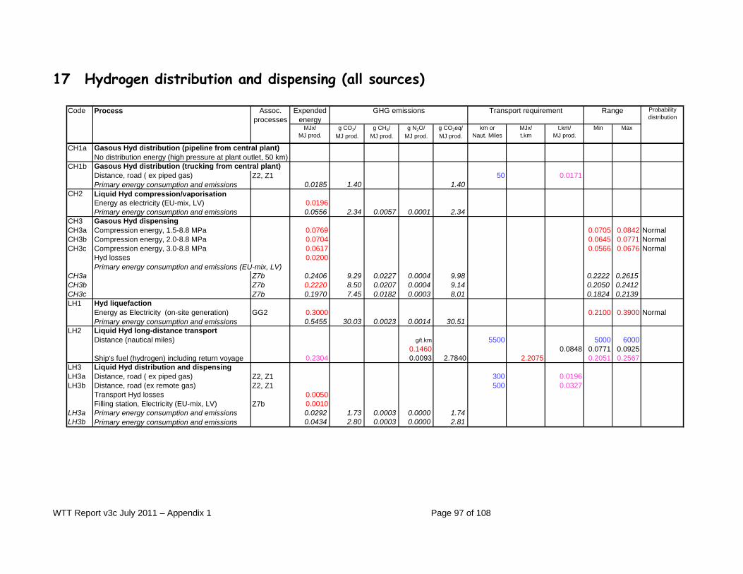
WTT Report v3c July 2011 – Appendix 1 Page 97 of 108
17 Hydrogen distribution and dispensing (all sources)
Code Process Expended energy
MJx/MJ prod.
g CO2/MJ prod.
g CH4/MJ prod.
g N2O/MJ prod.
g CO2eq/MJ prod.
km orNaut. Miles
MJx/t.km
t.km/MJ prod.
Min Max
CH1a Gasous Hyd distribution (pipeline from central plant)No distribution energy (high pressure at plant outlet, 50 km)
CH1b Gasous Hyd distribution (trucking from central plant)Distance, road ( ex piped gas) Z2, Z1 50 0.0171Primary energy consumption and emissions 0.0185 1.40 1.40
CH2 Liquid Hyd compression/vaporisationEnergy as electricity (EU-mix, LV) 0.0196Primary energy consumption and emissions 0.0556 2.34 0.0057 0.0001 2.34
CH3 Gasous Hyd dispensingCH3a Compression energy, 1.5-8.8 MPa 0.0769 0.0705 0.0842 NormalCH3b Compression energy, 2.0-8.8 MPa 0.0704 0.0645 0.0771 NormalCH3c Compression energy, 3.0-8.8 MPa 0.0617 0.0566 0.0676 Normal
Hyd losses 0.0200Primary energy consumption and emissions (EU-mix, LV)
CH3a Z7b 0.2406 9.29 0.0227 0.0004 9.98 0.2222 0.2615CH3b Z7b 0.2220 8.50 0.0207 0.0004 9.14 0.2050 0.2412CH3c Z7b 0.1970 7.45 0.0182 0.0003 8.01 0.1824 0.2139LH1 Hyd liquefaction
Energy as Electricity (on-site generation) GG2 0.3000 0.2100 0.3900 NormalPrimary energy consumption and emissions 0.5455 30.03 0.0023 0.0014 30.51
LH2 Liquid Hyd long-distance transportDistance (nautical miles) g/t.km 5500 5000 6000
0.1460 0.0848 0.0771 0.0925Ship's fuel (hydrogen) including return voyage 0.2304 0.0093 2.7840 2.2075 0.2051 0.2567
LH3 Liquid Hyd distribution and dispensingLH3a Distance, road ( ex piped gas) Z2, Z1 300 0.0196LH3b Distance, road (ex remote gas) Z2, Z1 500 0.0327
Transport Hyd losses 0.0050Filling station, Electricity (EU-mix, LV) Z7b 0.0010
LH3a Primary energy consumption and emissions 0.0292 1.73 0.0003 0.0000 1.74LH3b Primary energy consumption and emissions 0.0434 2.80 0.0003 0.0000 2.81
Assoc. processes
Transport requirementGHG emissions Range Probability distribution
WTT Report v3c July 2011 – Appendix 1 Page 98 of 108
CH1a/b Gaseous hydrogen distribution Hydrogen is available from the various producing plants at pressures generally above 3 MPa. This is considered sufficient for distribution through a local pipeline network over a distance of maximum 50 km, without additional compression energy. The resulting pressure at the refuelling station is taken at typically 2 MPa. Gaseous hydrogen can also be transported by road in high pressure cylinders (about 20 MPa, 0.45 t of hydrogen for 26 t of steel and composite material [Worthington 2000]). The compression energy for this is accounted for process CH2. The energy included here is for the operation of the truck. CH2 Liquid hydrogen vaporisation/compression Hydrogen delivered in liquid form to the refuelling station may have to be vaporised and compressed if the vehicles require compressed hydrogen. This process is less energy-intensive than compression of gaseous hydrogen, essentially as the liquid can be pumped to the required pressure before vaporisation [BOC 1997], [Linde 2001]. CH3 Gaseous hydrogen compression Gaseous is available at the refuelling station at a pressure of between 1.5 for a small scale on-site electrolyser and 3.0 MPa for on-site production via electrolysis. 2 MPa corresponds to piped hydrogen (see above). In the case of road transport of high pressure cylinders, the pressure is of course higher at the refuelling station but the total energy cost of compression remains essentially the same. LH1 Hydrogen liquefaction Liquefaction is a highly energy intensive process. Energy requirement figures vary within a wide range. One reason for this is that many of the existing liquefaction plants were not built with the objective of maximum energy efficiency as they are mostly relatively small and making hydrogen as a premium product for the chemical industry. Figures in the region of 0.35-0.40 MJe/MJ are not uncommon but experts agree that much lower figures down nearly 0.2 can be achieved [LBST 2001], [Quack 2001/1], [Quack 2001/2] have therefore taken a wide range with a square probability distribution. Note that this process refers to process GG2 i.e. electricity produced with a natural gas CCGT. In wood-based pathways electricity is assumed to be made on site also with wood. In such cases, although the energy requirement for liquefaction remains the same, the energy and GHG balances are different (more total energy and less GHG). LH2 Liquid hydrogen long-distance transport This process pertains to a scenario where hydrogen would be produced and liquefied at a remote location to be shipped to markets in specially built liquid hydrogen carriers. Such a so-called SWATH carrier has been proposed [Würsig 1996] and we have used the figures as quoted. The SWATH carrier would burn exclusively hydrogen.

WTT Report v3c July 2011 – Appendix 1 Page 99 of 108
LH3 Liquid hydrogen distribution This is envisaged exclusively by road. The average distance to cover varies with the scenario. Large reformers fed with LNG would have to be located near the coastal terminal, with potential higher distribution distances (500 km) than other central plants fed with more “local” material such as piped NG, wood or electricity (300 km). The liquid hydrogen road tanker is assumed to transport 3.5 t of hydrogen in a 24 t tank [Linde 1998]

WTT Report v3c July 2011 – Appendix 1 Page 100 of 108
18 Synthetic fuels distribution and dispensing (all sources)
Code Process Expended energy
MJx/MJ prod.
g CO2/MJ prod.
g CH4/MJ prod.
g N2O/MJ prod.
g CO2eq/MJ prod.
km orNaut. Miles
MJx/t.km
t.km/MJ prod.
Min Max
DS1 Syn diesel handling and loading (remote)Energy as Electricity (on-site generation) GG2 0.0008Primary energy consumption and emissions 0.0015 0.08 0.0000 0.0000 0.09
DS2 Syn diesel sea transportDistance (nautical miles) 5500 5000 6000Energy requirement as HFO for product carrier 0.2315 0.2105 0.2525 SquarePrimary energy consumption and emissions 0.00 0.0312 2.50 2.50 0.0284 0.0341
DS3 Syn diesel depotElectricity (EU-mix, LV) Z7b 0.0008Primary energy consumption and emissions 0.0024 0.36 0.0009 0.0000 0.39
DS4 Syn diesel distribution (blending component CD2/3/4 See conventional diesel processesDS5 Syn diesel distribution (neat)
Distance, Rail Z5, Z7a 250 0.0057Distance, road Z2, Z1 250 0.0061Primary energy consumption and emissions
DS5a Rail+Road 0.0100 0.6413 0.0003 0.0000 0.65DS5b Road only 0.0066 0.4995 0.0004 0.0000 0.51
Assoc. processes
Transport requirementGHG emissions Range Probability distribution
DS1 Synthetic diesel loading and handling (remote) This represents the energy required to store, handle and load the synthetic diesel near its (remote) production site. The assumed electricity consumption is that of a standard conventional diesel depot (see process CD3). This process (and the next one), are only relevant to GTL plants inasmuch as diesel from biomass is unlikely to be transported across large distances. The source of electricity is here deemed to be the gas-fired power plant part of the GTL complex (process GG2). DS2 Synthetic diesel sea transport Synthetic diesel can be transported in essentially standard product carriers (see process Z4). The distance considered here is typical of a trip from the Arab gulf to North West Europe (via Suez). The energy figure includes an allowance for the return trip. DS3 Synthetic diesel depot This is the same process as CD3. This energy is deemed to be spent at a receiving terminal.

WTT Report v3c July 2011 – Appendix 1 Page 101 of 108
DS4 Synthetic diesel distribution (blending component) Synthetic diesel is a valuable blending component for modern diesel and the limited quantities available are most likely to be used as such. In this case the product will enter the refinery system near the point of production. The applicable processes are thus the same as for conventional diesel (CD2/3/4). DS5a/b Synthetic diesel distribution (neat) The use of neat synthetic diesel in niche applications cannot be ruled out. Transport of neat synthetic diesel within Europe can be envisaged either by road, rail or a combination of both. The limited volumes involved would make pipeline transportation inappropriate. We have considered two scenarios depending on the synthetic diesel source. Material imported from remote plants would have to be transported from a small number of ports for which we consider an average distance of 500 km (split 50/50 between rail and road). Material manufactured within Europe would be more “distributed” and we have considered a distance of 250 km (road) as appropriate. The transport mode parameters are in accordance with processes Z5 and Z2.

WTT Report v3c July 2011 – Appendix 1 Page 102 of 108
Code Process Expended energy
MJx/MJ prod.
g CO2/MJ prod.
g CH4/MJ prod.
g N2O/MJ prod.
g CO2eq/MJ prod.
km orNaut. Miles
MJx/t.km
t.km/MJ prod.
Min Max
ME1 Methanol handling and loading (remote)Energy as Electricity (on-site generation) GG2 0.0018NG consumption and emissions 0.0033 0.18 0.0000 0.0000 0.19
ME2 Methanol sea transport (average of two distances)Distance (nautical miles) 5000 0.465 0.465Primary energy consumption and emissions Z3, Z4 0.0627 5.03 5.03 NormalDistance (nautical miles) 6000 0.558 0.558Primary energy consumption and emissions Z3, Z4 0.0753 6.04 6.04
ME3 Methanol depotElectricity (EU-mix, LV) Z7b 0.0018Primary energy consumption and emissions 0.0052 0.79 0.0019 0.0000 0.85
ME4 Methanol distribution and dispensingDistance, Rail Z5, Z7a 250 0.0126Distance, road Z2, Z1 250 0.0135Filling station, Electricity (EU-mix, LV) Z7b 0.0034Primary energy consumption and emissions
ME4a Rail+Road 0.0319 1.83 0.0018 0.0000 1.89ME4b Road only 0.0244 1.52 0.0010 0.0000 1.55DE1 DME handling and loading (remote)
Energy as Electricity (on-site generation) GG2 0.0013NG consumption and emissions 0.0024 0.13 0.0000 0.0000 0.13
DE2 DME sea transportDistance (nautical miles) gCO2/tkm 5500 0.358 0.326 0.391 NormalEnergy to DME carrier (as HFO) Z3 13.11 0.163Primary energy consumption and emissions 0.06343 5.09 5.09
DE3 DME depotElectricity (EU-mix, LV) Z7b 0.0013Primary energy consumption and emissions 0.0037 0.56 0.0014 0.0000 0.60
DE4a DME distribution and dispensingDistance, Rail Z5, Z7a 250 0.0088Distance, road Z2, Z1 250 0.0123Filling station, Electricity (EU-mix, LV) Z7b 0.0034Primary energy consumption and emissions
DE4a Rail+Road 0.0284 1.64 0.0015 0.0000 1.69DE4b Road only 0.0231 1.42 0.0010 0.0000 1.45
Assoc. processes
Transport requirementGHG emissions Range Probability distribution
ME1 Methanol handling and loading (remote) This process relates to the small amount of energy (electricity) required to handle methanol from a remote NG-based plant to the loading terminal, including loading onto a ship. The figures have been inferred from those listed for gasoline (process CG3). The electricity is assumed to come from the on-site gas-fired power plant.

WTT Report v3c July 2011 – Appendix 1 Page 103 of 108
ME2 Methanol sea transport Methanol can be transported in essentially standard product carriers (see process Z3). The distance considered here is typical of a trip from the Arab gulf to North West Europe (via Suez). The energy figure includes an allowance for the return trip. ME3 Methanol depot A small amount of energy is added to account for this intermediate handling step between unloading from the ship and further transport to customers. ME4a/b Methanol distribution and dispensing Transport of methanol within Europe can be envisaged either by road, rail or a combination of both. Pipeline transportation is not considered likely inasmuch as a dedicated pipeline system would be difficult to justify in all credible scenarios. Transporting methanol in the existing oil products pipelines is not a practical option for a number of reasons including, interface management, water contamination and corrosion issues. We have considered two scenarios depending on the methanol source. Methanol imported from remote plants would have to be transported from a small number of ports for which we consider an average distance of 500 km (split 50/50 between rail and road). Methanol manufactured within Europe would be more “distributed” and we have considered a distance of 250 km (road) as appropriate. The road tanker is assumed to transport 26 t of methanol in a 2 t tank. The transport mode parameters are in accordance with processes Z5 and Z2. The filling station energy requirement is inferred from the gasoline figure (see process CG4). DE1-4 DME distribution and dispensing These processes are similar to those for methanol with figures adapted to DME which is transported in compressed liquid form. DME is deemed to be carried on a ship similar to an LPG carrier [Kawasaki 2000]. The road tanker is assumed to transport 2 t of DME in a 20 t tank.
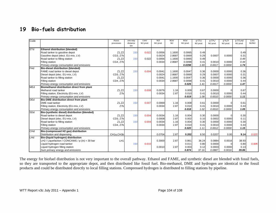
WTT Report v3c July 2011 – Appendix 1 Page 104 of 108
19 Bio-fuels distribution
Code Assocprocesses
one-waydistance
km
t.km/MJ prod.
MJ/ MJ prod.
MJx/MJ
MJx/MJ prod.
g CO2/MJ prod.
g CH4/MJ prod.
g N2O/MJ prod.
g CO2eq/MJ prod.
LossMJ/MJ
ETd Ethanol distribution (blended)Road tanker to gasoline depot Z1,Z2 150 0.022 0.0056 1.1600 0.0065 0.49 0.49Gasoline depot (elect. EU-mix, LV) CG3, Z7b 0.0024 2.8687 0.0069 0.29 0.0007 0.0000 0.31Road tanker to filling station Z1,Z2 150 0.022 0.0056 1.1600 0.0065 0.49 0.49Filling station CG4, Z7b 0.0034 2.8687 0.0098 0.41 0.0010 0.0000 0.44Primary energy consumption and emissions 0.0298 1.69 0.0017 0.0000 1.74
FAd Bio-diesel distribution (blended)FAME road tanker to diesel depot Z1,Z2 150 0.004 0.0041 1.1600 0.0047 0.36 0.0000 0.0000 0.36Diesel depot (elec. EU-mix, LV) CD3, Z7b 0.0024 2.8687 0.0069 0.29 0.0007 0.0000 0.31Road tanker to filling station Z1,Z2 0.0041 1.1600 0.0047 0.36 0.0000 0.0000 0.36Filling station CD4, Z7b 0.0034 2.8687 0.0098 0.41 0.0010 0.0000 0.44Primary energy consumption and emissions 0.026 1.41 0.0017 0.0000 1.47
MEd Biomethanol distribution direct from plantMethanol road tanker Z1,Z2 150 0.008 0.0076 1.16 0.009 0.67 0.0000 0 0.67Filling station, Electricity (EU-mix, LV) Z7b 0.0034 2.87 0.010 0.41 0.0010 0.0000 0.44Primary energy consumption and emissions 0.019 1.08 0.0010 0.0000 1.11
DEd Bio-DME distribution direct from plantDME road tanker Z1,Z2 150 0.007 0.0069 1.16 0.008 0.61 0.0000 0 0.61Filling station, Electricity (EU-mix, LV) Z7b 0.0034 2.87 0.010 0.41 0.0010 0.0000 0.44Primary energy consumption and emissions 0.018 1.02 0.0010 0.0000 1.05
SDd Bio-(synthetic diesel) distribution (blended)Road tanker to diesel depot Z1,Z2 150 0.004 0.0034 1.16 0.004 0.30 0.0000 0 0.30Diesel depot (elec. EU-mix, LV) CD3, Z7b 0.0008 2.87 0.002 0.10 0.0002 0.0000 0.11Road tanker to filling station Z1,Z2 150 0.004 0.0034 1.16 0.004 0.30 0.0000 0.0000 0.30Filling station CD4, Z7b 0.0034 2.87 0.010 0.41 0.0010 0.0000 0.44Primary energy consumption and emissions 0.020 1.11 0.0012 0.0000 1.15
CHd Bio-(compressed H2 gas) distributionDistribution and dispensing CH1a,CH3b 0.0704 2.87 0.202 8.50 0.0207 0.00 9.14 0.020
LHd Bio-(liquid hydrogen) distributionLH2 / Liquefaction / CONCAWE / p (in) = 30 bar LH1 0.3000 2.87 0.861 36.24 0.0884 0.0016 38.93Liquid hydrogen road tanker 150 0.010 0.011 0.80 0.0000 0 0.80 0.005Liquid hydrogen filling station 0.0010 2.87 0.003 0.12 0.0003 0.0000 0.13Sum primary energy and emissions 0.874 37.16 0.0887 0.0016 39.86
The energy for biofuel distribution is not very important to the overall pathway. Ethanol and FAME, and synthetic diesel are blended with fossil fuels, so they are transported to the appropriate depot, and then distributed like fossil fuel. Bio-methanol, DME and hydrogen are identical to the fossil products and could be distributed directly to local filling stations. Compressed hydrogen is distributed to filling stations by pipeline.

WTT Report v3c July 2011 – Appendix 1 Page 105 of 108
20 References References such as “[Source: xxx]" denote personal communications between CONCAWE/LBST and experts from member companies, not supported by a published document. The complete reference list is available in WTT Appendix 5.
WTT Report v3c July 2011 – Appendix 1 Page 106 of 108
European Commission EUR 24952 EN – Joint Research Centre – Institute for Energy Title: Well-to-Wheels Analysis of Future Automotive and Powertrains in the European Context Author(s): R. Edwards, J-F. Larivé, J-C. Beziat Luxembourg: Publications Office of the European Union 2011 – 108 pp. – 21 x 29.7 cm EUR – Scientific and Technical Research series – ISSN 1831-9424 ISBN 978-92-79-21395-3 doi:10.2788/79018 Abstract WELL-TO-WHEELS ANALYSIS OF FUTURE AUTOMOTIVE FUELS AND POWERTRAINS IN THE EUROPEAN CONTEXT The JEC research partners [Joint Research Centre of the European Commission, EUCAR and CONCAWE] have updated their joint evaluation of the well-to-wheels energy use and greenhouse gas emissions for a wide range of potential future fuel and powertrain options. This document reports on the third release of this study replacing Version 2c published in March 2007. The original version was published in December 2003.

WTT Report v3c July 2011 – Appendix 1 Page 107 of 108
How to obtain EU publications Our priced publications are available from EU Bookshop (http://bookshop.europa.eu), where you can place an order with the sales agent of your choice. The Publications Office has a worldwide network of sales agents. You can obtain their contact details by sending a fax to (352) 29 29-42758.

The mission of the JRC is to provide customer-driven scientific and technical support for the conception, development, implementation and monitoring of EU policies. As a service of the European Commission, the JRC functions as a reference centre of science and technology for the Union. Close to the policy-making process, it serves the common interest of the Member States, while being independent of special interests, whether private or national.
LB-N
A-24952-EN
-N