We examine drivers of cost overruns in Norwegian ... - CORE · PDF fileAmong the significant...

econstorMake Your Publication Visible

A Service of

zbwLeibniz-InformationszentrumWirtschaftLeibniz Information Centrefor Economics

Oglend, Atle; Osmundsen, Petter; Lorentzen, Sindre

Working Paper

Cost Overrun at the Norwegian Continental Shelf:The Element of Surprise

CESifo Working Paper, No. 5886

Provided in Cooperation with:Ifo Institute – Leibniz Institute for Economic Research at the University ofMunich

Suggested Citation: Oglend, Atle; Osmundsen, Petter; Lorentzen, Sindre (2016) : Cost Overrunat the Norwegian Continental Shelf: The Element of Surprise, CESifo Working Paper, No. 5886

This Version is available at:http://hdl.handle.net/10419/141863

Standard-Nutzungsbedingungen:

Die Dokumente auf EconStor dürfen zu eigenen wissenschaftlichenZwecken und zum Privatgebrauch gespeichert und kopiert werden.

Sie dürfen die Dokumente nicht für öffentliche oder kommerzielleZwecke vervielfältigen, öffentlich ausstellen, öffentlich zugänglichmachen, vertreiben oder anderweitig nutzen.

Sofern die Verfasser die Dokumente unter Open-Content-Lizenzen(insbesondere CC-Lizenzen) zur Verfügung gestellt haben sollten,gelten abweichend von diesen Nutzungsbedingungen die in der dortgenannten Lizenz gewährten Nutzungsrechte.

Terms of use:

Documents in EconStor may be saved and copied for yourpersonal and scholarly purposes.

You are not to copy documents for public or commercialpurposes, to exhibit the documents publicly, to make thempublicly available on the internet, or to distribute or otherwiseuse the documents in public.

If the documents have been made available under an OpenContent Licence (especially Creative Commons Licences), youmay exercise further usage rights as specified in the indicatedlicence.

www.econstor.eu

Cost Overrun at the Norwegian Continental Shelf: The Element of Surprise

Atle Oglend Petter Osmundsen Sindre Lorentzen

CESIFO WORKING PAPER NO. 5886 CATEGORY 13: BEHAVIOURAL ECONOMICS

MAY 2016

An electronic version of the paper may be downloaded • from the SSRN website: www.SSRN.com • from the RePEc website: www.RePEc.org

• from the CESifo website: Twww.CESifo-group.org/wp T

ISSN 2364-1428

http://www.ssrn.com/

http://www.repec.org/

http://www.cesifo-group.de/

CESifo Working Paper No. 5886

Cost Overrun at the Norwegian Continental Shelf: The Element of Surprise

Abstract We examine drivers of cost overruns in Norwegian development projects in the oil and gas sector. The multivariate longitudinal econometric analysis employs a unique and detailed dataset consisting of 80 different projects between 2000 and 2015. Among the significant results, we find that the unexpected change in economic activity has a positive effect on the overruns; there is a considerable positive momentum in the transitional cost overruns; more experienced operators tend to incur less overruns; finally, that the size of the investment of the projects has a positive impact on the overruns. Further, we find evidence that the current economic activity matters to an extent, but it is the unexpected change in activity that is the pivotal factor.

JEL-Codes: C510, D220, C310.

Keywords: cost overrun, cost estimation, estimation error.

Atle Oglend University of Stavanger

Norway – 4036 Stavanger [email protected]

Petter Osmundsen University of Stavanger

Norway – 4036 Stavanger [email protected]

Sindre Lorentzen

University of Stavanger Norway – 4036 Stavanger [email protected]

1 Introduction Delivering at or below the estimated cost is considered a pivotal criterion, alongside quality, delivery

on schedule and production attainment, for evaluating the success of project execution. A cost

overrun, defined as the inflation-adjusted deviation between realised and estimated costs, may

provide some information about the quality of the ex ante decision to undertake the project in

question. Evaluating the available set of investment opportunities and actively determining which

projects to implement represents a core activity for companies. The desirability of a particular

project is evaluated by companies on the basis the profitability metric they use, such as net present

value (NPV) or the internal rate of return. If an oil and gas company is cash constrained, it will use a

profitability metric which allows for capital rationing, such as the NPV index or the break-even price

(often supplemented by other criteria like production targets and strategic issues). Taking this

approach allows a company to achieve an optimal allocation of available capital. Where cost

estimate bias is present, however, the profitability ranking of the investment opportunity set will be

distorted and the company will allocate capital sub-optimally. Cost estimate bias is detrimental to the

value of companies, and reducing it would allow companies to take better-informed decisions which

thereby generate more value.

Cost overruns have been extensively examined in the literature. See Cantarelli et al (2010) for an

excellent overview. Prior to the seminal work of Flyvbjerg, however, the research was predominantly

non-empirical. Flyvberg’s papers (Flyvbjerg et al, 2002, 2003, 2004; Flyvbjerg and Stewart, 2012)

introduce crucial empirical insights through highly relevant case studies in public transport. In this

paper, we extend his work to the oil and gas industry and also complement his empirical methods.

Whereas he applies univariate cross-sectional regressions with few explanatory variables, we utilise a

more rigorous methodology with longitudinal multivariate regressions. We benefit from a unique

and detailed data set on oil projects in Norway, where oil companies are required to make detailed

and frequent project reports to the government. Our data come from the national budget and the

Norwegian Petroleum Directorate (NPD).

The purpose of this research is twofold. First, we aim to describe the characteristics of cost overruns

in offshore projects on the Norwegian continental shelf (NCS) in order to elucidate whether this

sector confirms with results obtained for other sectors. This is achieved by inspecting the

distributional moments of the cost overruns both on an aggregate level and across various sub-

samples. This approach can reveal more of the inner dynamics of the overruns. Second, we attempt

to identify a model with explanatory power for the cost overruns so that companies can be equipped

with tools to make better investment decisions. The contribution of this paper is as follows: (1) we

analyse a sector which is relatively untouched in the literature and (2) we utilise a more rigorous

methodology with longitudinal multivariate regressions. A wide range of variables are applied as

regressors. We test, for example, various proxies for the level of economic activity, technical project

complexity, project ownership characteristics and operator experience, as well as variables capturing

the inner dynamics of the cost overrun are tested.

We have data from different points of time during project execution, with updated cost estimates.

On inspecting the distributional moments of the cost overruns, it appears that the results mostly

conform with findings in other sectors such as public transport and construction. The distribution

exhibits both positive mean and skewness. Further, the initial in-progress cost overruns (the first

panel data observation of a cost overrun for a given project) appear to conform more to white-noise

than does the realised cost overrun (the last panel data observation). The transitional cost overrun –

the percentage change between each observation of the cost overrun – exhibits a high degree of

persistence and even momentum. Indications therefore exist that, once a cost overrun emerges in a

project, it will tend to continue to grow throughout the project. A project which stumbles in the

beginning therefore continues to have problems, and the oil companies seem unable to update their

forecasts accordingly. Interestingly enough, there are no indications that cost estimates became

more accurate during the 14 years covered by the sample. We find no learning effects where cost

estimating is concerned.

The observed persistence and momentum of the transitional cost overrun are interesting. First, given

a fully rational agent estimating costs throughout the execution of a project, all available information

should be discounted at each control estimate. As a consequence, the transitional cost overrun

should follow a random walk. The observed persistence and momentum in the transitional cost

overrun appear to be a deviation from the random walk model and thereby indicate that the agents

are not fully discounting all the information. Whether the failure to account properly for all available

information reflects random error, less comprehensive cost estimate procedures once projects have

been sanctioned, or an attempt to hide cost overruns by spreading them across a longer time interval

is unknown. Second, if we assume that project tasks are carried out uniformly throughout the

execution period, or at least that progress is increasing monotonically with time, then the challenge

of estimating the cost should be declining. In other words, since the proportion of the project cost

which has already been implemented is increasing, the uncertainty is decreasing. The finding that

transitional cost overruns tend to increase as the underlying estimate uncertainty falls seems

incompatible with random error and might be more in line with insufficient efforts to update costs or

with strategic misrepresentation.

Regression analysis appears to produce a unified story of the driving force behind a cost overrun –

deviation from the expected development cost is a tale of the unexpected. Technical complexity

appears to have no significant effect on the overruns. This is presumably attributable to the limited

unexpected changes in variables, such as ocean or drilling depth. Furthermore, the level of economic

activity in the petroleum sector as such has a significant, but limited, effect on the cost overrun. The

major driver is unexpected change in the level of economic activity. We also find that the local

project experience of the operating company reduces cost overruns.

The remainder of this paper is organised in the following way. Section 2 presents the literature.

Section 3 elaborates on the data utilised. Analysis of the distributional moments of the dependent

variable “cost overrun” and the explanatory variable “transitional cost overrun” is undertaken in

section 4. Section 5 presents the results from both univariate and multivariate regression analysis,

and section 6 discusses the results obtained. Finally, section 7 summarises and concludes.

2 Literature review Several prominent theories attempting to explain why costs overrun can be found in the literature.

According to Flyvbjerg et al (2002), the plethora of cost overruns which have emerged from the

literature can be classified into four distinct categories of theories: technical, economic, psychological

and political.

The technical approach to explaining cost overruns postulates that higher than expected cost is a

function of forecasting errors attributable to imperfect methods and data. If cost escalation can be

attributed to technical aspects, it can be argued that negative and positive cost overruns should be

equally likely. In other words, the distribution of overruns should be symmetric and be centred, on

average, around zero. Furthermore, since forecasting and estimating techniques incrementally

improve as experience is accumulated, the average size of the overruns should be declining over time

and converging towards zero. Where the economic theory of cost overruns is concerned, the

existence of an economic incentive for the agents estimating costs to understate the costs

deliberately has been postulated. Assuming this to be true, the expectation is that the distribution of

cost overruns should be asymmetrical and the mean time invariant. The psychological theories

regard a cost overrun as the effect of cognitive bias and faulty decision-making heuristics in the mind

of the agent doing the estimating. As with the economic approach, the psychological explanation

predicts that the distribution ought to be asymmetrical. Unlike with economic thinking, however, the

mean should approach zero as these biases become more elucidated and better understood. Finally,

the political explanation is similar to the economic one in the sense that the cost overrun is believed

to be the result of deliberate deception motivated, as its designation implies, by political rather than

economic reasoning. As a result, predictions regarding distribution are equivalent to those generated

by the economic approach.

Table 1: Categories of cost overrun theories This table showcases the predictions derived from the four categories of theories concerning the statistical moments of a cost overrun and their temporal stability.

Theory categories Distributional predictions

Mean Skewness Time invariability

Technical: 𝜇 = 0 𝑠 = 0 lim𝑡→∞

𝜇𝑡 = 0

Economic: 𝜇 ≠ 0 𝑠 ≠ 0 lim𝑡→∞

𝜇0 = 𝜇𝑡

Psychological: 𝜇 ≠ 0 𝑠 ≠ 0 lim𝑡→∞

𝜇𝑡 = 0

Political: 𝜇 ≠ 0 𝑠 ≠ 0 lim𝑡→∞

𝜇0 = 𝜇𝑡

Flyvbjerg’s classification of theories is appealing and illuminating. To elaborate further, it is difficult

to induce agents to be truthful in revealing their intent to deceive decision-makers by manipulating

the cost estimates. This makes data availability challenging, and the proposed relationships cannot

be evaluated empirically. The analysis of the different categories of theories in the literature has

been confined to an inspection of the cost overrun’s distributional moments in order to verify

whether they adhere to a specific category of predictions. This approach might be a good point of

departure, but needs to be augmented in the case where two or more hypotheses yield equivalent

predictions. Both the economic and the political hypotheses, for example, yield the same predictions

for mean, skewness and time-variability (see Table 1). If the cost overrun sample is confined to a

short time range, it also becomes challenging to distinguish the two former theories from the

psychological explanation. Another theory which produces the same distributional predictions is

sample selection bias (Jørgensen, 2013; Eliasson and Fosgerau, 2013). If costs are estimated with a

symmetric and random bias, then (ceteris paribus) a project with a negative cost bias will be

favoured over a project with positive bias, since the former will artificially inflate the NPV of the

investment. Undertaking a project with a negative cost estimate bias will induce a cost overrun and,

conversely, a positive bias will result in a cost underrun. By selecting investments with the highest

estimated NPV, the company will actively select projects with a negative bias and the distribution of

cost overruns will consequently exhibit both a positive mean and skewness.

Given the inability to elicit information on the intentions of agents estimating costs, performing a

proper empirical regression analysis is challenging. As a direct consequence, the literature has aimed

predominantly at exploring the technical category of cost overrun theories. A review of 240 articles

from the proceedings of the 22nd conference of the International Project Management Association

(IPMA) in 2008 reveals a great many different success factors in the technical category which can

affect project execution performance. These range from such well-known aspects as project

complexity to the nutritional properties of the project manager’s lunch. These factors predominantly

involve a level of detail which requires researchers to perform an in-depth qualitative case study.

Among the more easily available factors, several variables can be addressed within a more general

research design. These include project complexity, project manager competence and various

characteristics of project ownership.

A consensus prevails that complexity is one of the main cost overrun drivers (McKenna et al, 2006)

and it has generally been established that cost overruns increase with complexity. This positive

correlation between complexity and project performance could have several interpretations. It could,

for example, be the case that the absolute level of complexity is not necessarily what matters, but

the unexpected level of complexity which project managers encounter during project execution.

Staats et al (2012) argue that such underestimating increases with the degree of complexity, so cost

overruns should be more frequent in complex projects. Second, Grieco and Hogarth (2009) find that

people tend to be more overconfident when estimating complex tasks and, conversely, less confident

with comparatively simpler tasks. Complexity is a broad concept, and could encompass a variety of

different aspects. To address this point of view, Baccarini (1996) disaggregates complexity into

technical and organisational dimensions. Technical and organisational complexity may affect project

cost overruns to varying degrees. According to Bosch-Rekveldt and Mooi (2008), for instance,

companies tend to invest more effort in addressing technical complexity rather than complex

organisational issues such as coordination and timing. Companies might consequently be less

prepared to handle the latter when they emerge.

Complexity of the task is arguably just part of the explanation for cost overruns. The competence of

the project management is likely to be an additional determinant. As such, the ability of companies

to predict future costs can be viewed as the amalgam of both the complexity of the project and their

expertise and experience. Competence is generally challenging to quantify, but Remington and

Pollack (2008) report that the experience of management matters. More specifically, Osmundsen et

al (2010) find an empirical relationship between offshore productivity and experience in terms of the

accumulated number of projects which the operator had participated in.

Table 2: Cost overrun theory

Theory Author

Technical:

Managerial incompetence

Morris and Hough (1987) Fouracre et al (1990) Nijkamp and Ubbels (1999) Love et al (2005) Bordat et al (2004) Olawale and Sun (2010)

Contract form Arvan and Leite (1990) Mansfield et al (1994)

Uncertainty Hall (1982) Project complexity Odeck (2004) Financial incentives Pickrell (1992) Newtonian world assumption Flyvbjerg et al (2003)

Scoop creep (evolution theory) Lee (2008) Love et al (2012) Gil and Lundrigan (2012)

Economic:

Economic self-interest Flyvbjerg et al (2003) Public interest Flyvbjerg et al (2003)

Psychological:

Optimism bias (planning fallacy)

Kahneman and Tversky (1977) Weinstein (1980) Buehler et al (1994) Kahneman and Lovallo (1993) Mackie and Preston (1998) Flyvbjerg (2008)

Prospect theory Kahneman and Tversky (1979) Dunning-Kruger effect Kruger and Dunning (1999)

Political:

Strategic misrepresentation (deception)

Wachs (1982) Wachs (1987) Pickrell (1989) Fouracre et al (1990) Wachs (1990) Flyvbjerg et al (2002) Bruzelius et al (2002) Altshuler and Luberoff (2003)

The explanatory variable most frequently utilised for cost overruns is project size. That probably

reflects the independence of this variable from context – that is, project size is applicable regardless

of the sector under consideration. In many ways, the size of the project’s investment might be

regarded as a proxy for its complexity . The ex ante expectation is consequently that larger projects

should incur more cost overruns. However, the literature appears to present conflicting findings on

the empirical effect of size on project cost overruns. Heemstra and Kusters (1991), Gray et al (1999),

Hatton (2007), Moløkken-Østvold et al (2004), Sauer et al (2007), Yang et al (2008) and Dantata et al

(2006), for instance, find a positive relationship between the two aforementioned variables.

However, Odeck (2004), Hill et al (2000), Bertisen and Davis (2008), Creedy (2006) and Cantarelli

(2011) identify a negative relationship. Finally, Van Oorschot et al (2005) and Flyvbjerg et al (2004)

find no relationship significantly different from zero. Jørgensen et al (2012) offers a possible

explanation for the observed differences in the literature. In their view, these can partly be explained

by variations in the proxy for project size. The literature tends, for example, to use the ex ante

estimated project cost and the ex post realised cost interchangeably. However, these two proxies

might not be perfectly correlated, and the empirical effect of project size might consequently tend to

differ across measures.

While the literature presented so far has investigated cost overruns regardless of sector and country,

these factors probably have an impact. Empirical literature concerning cost overruns on the NCS is

limited. However, several case studies and reports have been published during recent decades.

Among the few empirical studies, a paper by Sandberg and Hetland (2008) on cost overruns in

offshore projects on the NCS makes several noteworthy findings. First, the size of the investment in a

project has a positive effect on cost overruns. Small projects tend to have little or no overrun, while

mega developments (costing more than USD 1 billion) have a considerably higher risk of this. Second,

the business cycle measured by oil prices does not appear to have an impact on a project’s cost

overrun. Finally, risk regimes occur in the data – periods of tranquillity and turmoil can be identified.

Table 3: Case studies with offshore projects on the NCS

Study Period Number of projects studied

Investment Committee 1994-1998 13 Norwegian Petroleum Directorate 2006-2008 5 Office of the Auditor General 1995-1996 3

The Ministry of Petroleum and Energy appointed the Investment Committee in 1998 to analyse cost

overrun drivers on the NCS. The committee conducted an in-depth study of 13 development projects

on the NCS between 1994 and 1998. Among several noteworthy findings, various causes for overruns

were identified. First, the committee believes that the initial cost estimate presented in the plan for

development and operation (PDO) was based on unrealistic assumptions attributable to exaggerated

optimism. By extension, that prompted unjustified extrapolations of positive trends for input prices

and efficiency. Second, the project management had insufficient understanding of uncertainty and

risk. Third, planning by the project management before project execution began was inadequate.

Fourth, the availability of mobile drilling rigs and workers with high-level expertise had generally

been underestimated, which caused delays and cost overruns. In addition, excess demand meant

input prices were higher than expected. Fifth, shifts and advances in technology which had not been

taken into account introduced risks and uncertainties which were not planned for sufficiently. Finally,

it was suggested that the type and form of the contract between the project operator and the

contractor have a distinct impact on execution success.

An investigation of petroleum projects on the NCS by Norway’s Office of the Auditor General reveals

some of the drivers for cost overruns. Three projects pursued between 1995 and 1996 were

evaluated. The main cause of the cost overruns experienced appeared to be that plans were not

sufficiently developed before execution. As a result, topside structures turned out to be heavier than

intended and an infeasible technical design was replaced with more expensive alternatives. Variation

orders during project execution proved costly.

At the request of the Ministry of Petroleum and Energy, the NPD evaluated five projects executed on

the NCS with an investment cost of more than NOK 10 billion between 2006 and 2008. The NPD was

able to identify several possible cost overrun drivers . First, it argued that too little time was spent on

front-end engineering design (Feed) – ie, planning before project execution – because of ambitious

schedules. Consequently, the project plans often lacked sufficient detailing for costs to be accurately

estimated. Second, the project management lacked good routines for handling new information.

More specifically, data of this kind with the potential to cause changes in the technical aspects of the

project tended to be ignored because they would cause delays. However, ignoring this information

did not solve the problem. Instead, it emerged later in the project to cause a cost overrun. Third,

failures by the various subcontractors to deliver on schedule and to the specified quality/quantity

were a prominent source of cost overruns. The NPD speculated that this reflected a lack of

experience by the contractors or faulty prequalification. Fifth, inefficient follow-up caused errors in

contract specifications and consequent cost overruns and delays. According to the report, it was

unclear whether the primary driver was poor management quality or a lack of understanding of

Norway-specific regulations and standards. Finally, a causal link was suggested between the level of

activity in the economy and cost overruns. In other words, when activity was high, input prices

increased and bottlenecks appeared in crucial inputs.

3 Data The data set utilised in this paper consists of 80 different petroleum projects with 238 longitudinal

observations on the NCS between 2000 and 2013. All data were extracted from publicly available

sources. Pursuant to section 4, sub-section 2 of the 1997 Petroleum Act, all companies operating on

the NCS are obliged to submit a PDO (plan for development and operation) to the government for

approval before a project can be initiated. Information from the PDO was accessed through the

national budget and the Facts publication from the NPD. The cost estimates primarily utilised for

computing cost overruns as the dependent variable were extracted from the Norwegian national

budget, and the various independent variables from the NPD. See Tables 4 and 5 for a full list of all

explanatory variables, with the first of these presenting factors common to the various projects and

the second listing project-specific factors.

Ex ante the regressions analysis, the following expectations emerge for the relationship between the

dependent and independent variables. First, where oil and gas prices are concerned, these variables

are pro-cyclical with the business cycle. At times when economic activity is high, prices tend to rise

and access to key input materials tends to become limited. Consequently, it seems reasonable to

expect a positive relationship between commodity prices and cost overruns. Similar arguments can

be made for both aggregate investment on the NCS and the number of employees in the sector.

Second, a positive relationship can be expected with the various surprise variables for economic

activity. The surprise is defined here as the relative deviation in a macro variable from the ex ante

expectation, where the expectation is based on the assumption of a random walk. If the macro

variables are positive, then their respective surprise variables should behave similarly.

Third, it can be argued that idiosyncratic company variables affect the cost overrun in so far as they

either express the complexity of the project or come as a surprise to the company implementing the

project. In other words, the greater the complexity, the more probable is the possibility of errors and

mistake and the greater the chance of failing to include all relevant costs in the initial estimate. Both

the project size variables and the absolute size of the investment, and the technical aspect of

ocean/drilling depth and reservoir size, might serve as a proxy for the complexity of the project, and

a positive relationship with the cost overrun can consequently be expected. Fourth, the geographic

location of the project is expected to have an impact since the distance to infrastructure and

knowledge about area geology may vary with the location. Without performing a more detailed

analysis, however, it might be difficult to establish an expectation about the effect each location has

on the prevalence of cost overruns. Fifth, a relationship might exist between how far the company is

currently along with the project and the cost overrun. Since cost overrun is arguably cumulative, a

positive relationship can be expected. Finally, a distinct possibility exists that the ownership of the

project and the quality of the agent implementing it has an effect on its success in terms of cost

overrun. The number of rights holders and the concentration of ownership between them might be

an overrun driver. On the one hand, a large number of owners could provide greater access to

unique expertise. On the other, this could produce a more bureaucratic and cumbersome process.

The net effect of this variable is therefore unknown ex ante. Furthermore, the dispersion or

concentration of ownership might have similarly contrasting effects. Greater ownership balance may

reduce opportunities for sub-optimal solutions, but cause slower progress. Where the operator – the

company formally implementing the project on the behalf of the rights owners – is concerned, it

seems reasonable to expect that those with more experience tend to have fewer cost overruns on

their projects.

Table 4: List of common variable factors

Variable name short

Variable name long

Description of variable

Expected relationship

GasPrice Gas prices Natural gas (European import) price on an annual basis aggregated as the average monthly price

↑

GasPriceSur Gas price surprise Relative difference between the natural gas price in the current year and at the time of the PDO

↑

OilPrice Oil prices Price of Brent crude oil on an annual basis aggregated as the average monthly price

↑

OilPriceSur Oil price surprise Relative difference between oil price in current year and at the time of the PDO on the NCS

↑

RigRates Rig rates Rig rates on the NCS on an annual basis

↑

RigRateSur Rig rate surprise Relative difference between rig rates on the NCS in the current year and at the time of the PDO

↑

SecEmp Sector employees Number of Employees in the petroleum sector in Norway

↑

SecEmpSur Sector employee surprise

Relative difference in number of employees in the petroleum sector in Norway in the current year and at the time of the PDO

↑

SecInvest Sector invest Annual investment on the NCS in NOK million

↑

SecInvestSur Sector invest surprise Relative difference in investment on the NCS in the current year and at the time of the PDO

↑

Table 5: List of idiosyncratic variables

Variable name short

Variable name long

Description of variable

Expected relationship

BS Barents Sea Dummy variable for the Barents Sea

↑/↓

CNS Central North Sea Dummy variable for the Norway’s central North Sea sector

↑/↓

DrillingDepth Drilling depth Distance from the seabed to the reservoir in meters

↑

Exp Experience Total number of operatorships held by the project operator

↓

MegaPro Mega project

Dummy variable for projects with an investment size at the time of the PDO exceeding NOK 15 billion (109)

↑

NNS Northern North Sea Dummy variable for Norway’s northern North Sea sector

↑/↓

NoS Norwegian Sea Dummy variable for the Norwegian Sea

↑/↓

OceanDepth Ocean depth Distance from sea surface to seabed in meters

↑

OwnCon Ownership concentration The Herfindahl–Hirschman Index showing the squared sum of the interest among the rights owners

↑/↓

ProInvestStart Project investment size Investment size of the project at the time of the PDO in NOK millions

↑

RightsOwners Rights owners Number of rights owners in the project

↑/↓

ReservVol Rersvoir volume Size of the reservoir in oil equivalent in cubic meters (m3)

↑

SNS Southern North Sea Dummy variable for the Norway’s southern North Sea sector

↑/↓

4 Distributional analysis Considerable insight can be gained by simply evaluating the distributional moments and temporal

stability of the cost overrun. This part of the paper conducts a distributional analysis of the main

variables of interest. Sub-section 4.1 delves into the cost overrun, both on an aggregate level and

across temporal sub-samples. Sub-section 4.2 conducts a similar analysis with the transitional cost

overrun.

4.1 Cost overrun We define cost overrun in this article as the relative inflation-corrected difference between cost

estimates at times 0 and t. Unlike most studies, this data set consists of panel data rather than cross-

sectional information. That necessitates making a further distinction between completed and

incomplete projects. If the project is still in progress, then the cost at time t is a current control

estimate. Since the project has not been fully completed, the cost overrun is only tentative and may

be corrected later. We therefore label a cost overrun calculated from a control estimate as an in-

progress cost overrun. If the project has been fully implemented, however, the cost refers to its

realised cost.

The distinction between in-progress and realised cost overruns comes with a caveat. A few of the

projects in the sample have yet to be finished, and the latest observed cost estimate is referred to in

this case as the realised cost, alternatively as in-progress. An additional point of contention is the

timing of the initial estimate. From a decision-making point of view, cost overrun is a criterion for

evaluating success and, as such, the estimate available at the time of the decision is the only relevant

point of reference for computing it. We therefore opt to utilise the PDO estimate as our initial

estimate. An alternative approach to timing the initial estimate will be considered in sub-section 4.2

below.

𝐶𝑜𝑠𝑡𝑂𝑣𝑒𝑟𝑟𝑢𝑛 =

{

𝐶𝑜𝑠𝑡𝑇𝐸0(𝐶𝑜𝑠𝑡𝑇)

− 1 𝑖𝑓 𝑡 = 𝑇

𝐸𝑡(𝐶𝑜𝑠𝑡𝑇)

𝐸0(𝐶𝑜𝑠𝑡𝑇)− 1 𝑖𝑓 𝑡 < 𝑇

(1)

A visual inspection of the distribution of the cost overrun reveals that the data predominantly

conform to ex ante expectations on its statistical moments. See Figure 1. First, the mean is non-zero,

since the average cost overrun is 21 per cent, and there consequently appears to be a negative bias

on average in the cost estimate. Since the portfolio of 80 investment projects covered an overall

initial budget of NOK 973.8 billion, the cost overrun in absolute numbers represents considerable

capital. Second, the standard deviation is 0.42, and it therefore appears that more than five per cent

of the projects fall outside the ±20 per cent interval commonly utilised. In this case, 34 of the projects

were realised with a cost overrun outside the interval. Third, a positive skewness exists in the

distribution, indicating that more projects have a cost overrun than an underrun. As a matter of fact,

64 of 80 projects were realised with a cost overrun. Finally, the distributions exhibit a leptokurtosis of

19.53, which again implies that the proportion of projects within the predefined confidence interval

is smaller than with a normal distribution. Based on the observed distributional moments of the cost

overruns, it appears prudent to conclude that a deviation exists from the symmetric white noise

which ought to be present in the cost estimate. Before concluding that systematic bias exists,

however, it might be useful to consider that not all overruns are equally important. An in-progress

cost overrun is of little consequence, for example, if budgetary control can be restored later in the

project so that the realised cost does not deviate from the original estimate.

Figure 1: Cost overrun distribution

An investigation of the distributional characteristic and temporal stability of a cost overrun can help

to illuminate the potential drivers of the variable in question. Given that the cost overrun is observed

several times across the execution of the project, some interesting characteristics can be observed.

By differentiating between the initial in-progress and the realised cost overrun, the distribution’s

statistical moments can be seen to diverge. According to Table 6, the distribution of the initial

overrun exhibits a positive mean, positive skewness and leptokurtosis. For its part, the distribution of

the realised cost overrun displays a comparably greater mean, skewness, leptokurtosis and standard

deviation. It thereby appears that a cost overrun tends to accumulate throughout the execution time

and that the cost estimates deteriorate over time. Furthermore, as previously established in section

2 (see Table 1), these characteristics suggest that a cost overrun is not exclusively caused by technical

factors. In other words, the distribution of the overrun is consistent with the predictions of the

psychological, economic and political theories. However, whether a non-technical cause is really

behind the observed distributional moments cannot be verified exclusively by observing the cost

overrun.

Table 6: Summary statistics for cost overrun

Statistics Initial in-progress cost

overrun Realised cost overrun Cost overrun

Count 79 79 238 Mean 0.04 0.24 0.21 Std 0.12 0.49 0.43 Min 0.21 −0.67 −0.71 Max 0.59 2.93 2.93 Kurtosis 6.09 15.22 19.53 Skewness 1.31 3.28 3.6 >0 44 64 55 Outside ± 0.20 4 34 82

01

23

45

De

nsity

-1 0 1 2 3Cost overrun

Mean = .21 Std dev =.43 Skew = 3.6 Kurt = 19.53

Figure 2: Cost overrun histogram This figure display histogram plots for relative cost overruns in petroleum projects on the NCS between 2000 and 2013. Sub-figures (a) show the initial in-progress cost overrun and (b) the realised cost overrun. Sub-figure (c) combines both (a) and (b).

(a) Initial in-progress overrun (b) Realized overrun

(c) Initial in-progress and realized cost overrun

An interesting question proposed by Flyvbjerg et al (2002, 285) is “[. . .] whether project promoters

and forecasters have become more or less inclined over time to underestimate the costs of [. . .]

projects”. Where panel data is concerned, differentiating between global time and local project

execution time is crucial. Since cost overruns predominantly tend to accumulate throughout projects,

it would be misleading to compare the end phase of a project at time t with a newly started project

at time t + 1. Ignoring this pitfall could potentially produce an erroneous downward or upward trend.

With this consideration in mind, a scatter plot is constructed between the cost overrun and time for

both the initial in-progress and realised overruns in order to explore the temporal development of

cost estimate accuracy.

05

10

15

Den

sity

-.2 -.1 0 .1 .2 .3Initial in-progress cost overrun

0.5

11

.52

Den

sity

-1 0 1 2 3Realized cost overrun

05

10

15

20

Den

sity


Initial in-progress

Realized

Figure 3: Temporal development of cost overruns This figure presents scatter plots between cost overrun and time for both the initial in-progress cost overrun (a) and the realised cost overrun (b).

As Figures 3 (a) and (b) show, no discernible trend appears to exist in either direction for cost

overrun cases. Regressing cost overrun on time fails to produce any relationship significantly

different from zero. In line with the reasoning of Flyvbjerg et al (2002), this result is indicative of a

non-technical or non-psychological driver. However, it is arguable that the period covered by the

data is too short to reveal any significant effect from learning, so that no improvement occurs in the

cost estimate techniques. Another possibility is that innovation is so rapid that former experience

quickly becomes outdated. These alternatives cannot be evaluated exclusively by observing the cost

overrun. In a formal regression analysis, however, the learning effect associated with the

accumulated experience can be used to conduct further investigations of this proposed alternative

explanation. See sub-section 5.2.

4.2 Transitional cost overrun An interesting argument frequently voiced in the wake of an emerging cost overrun is that the initial

estimate is not relevant. Changes in the scope of the project, for instance, will invalidate the original

estimate presented when the decision to proceed with the project was taken. A later estimate should

therefore be used, which will change the size of the cost overrun incurred. This is a compelling and

convenient tactic to avoid criticism, but does it fundamentally change the distributional behaviour of

a cost overrun? Owing to limitations in the data set, however, the scope of the projects covered is

unknown. As a result, any changes in the project cannot be identified. This restriction can be

overcome by pushing the argument to its limit. If the project scope is changing throughout, the cost

overrun should be computed as the relative difference between two sequential control estimates. To

introduce some terminology, we introduce 𝐶𝐶𝐸𝑡/𝐶𝐶𝐸−1 − 1 as the transitional cost overrun

(TraCOt) for time t. This is the best we can do in accommodating the counterargument of changing

scope. Looking at the transitional cost overrun for the whole sample, the average overrun appears,

as expected, to be significantly lower than the overall one. It is worth noting that the behaviour of

the distribution remains the same. In other words, although lower, the average is still significantly

greater than zero. However, the skewness and kurtosis cannot be said to differ significantly from the

distribution of the overall cost overrun. In short, therefore, changing the reference point for

calculating the cost overrun does not reduce the problem of the prevalence of estimate error.

-.2

-.1

0.1

.2.3

Initia

l in

-pro

gre

ss c

ost ove

rrun

2000 2005 2010 2015

beta = -.003 (p-value = .1095)

-10

12

3

Initia

l in

-pro

gre

ss c

ost ove

rrun

2000 2005 2010 2015

beta = .019 (p-value = .1363)

Figure 4: Distribution of transitional cost overrun

Table 7: Summary statistics transitional cost overrun

Count Mean Std Min Median Max Skew Kurt

238 0.0727 0.1599 −0.7368 0.0447 1.4157 1.7532 27.5319

While using the transitional cost overrun to test the credibility of the argument about changing scope

is fascinating, this measure has a far more interesting use. Specifically, since the transitional cost

overrun essentially expresses the change between each control estimate, it can be used to illuminate

the efficiency of information updating. To appreciate this, it is useful to reflect how the uncertainty in

the estimates is developing throughout project execution. According to well-established theory, the

uncertainty associated with each incremental control estimates should be declining. Two

explanations are possible. One is that the proportion of tasks already fulfilled for each progressive

control estimate is increasing and the overall uncertainty is consequently decreasing, since no

uncertainty exists about the completed part of the project. The other is that the distance in time to

tasks which have yet to be implemented is decreasing – in other words, the relevant information set

is increasing. Presumably, the larger the information set, the greater the accuracy of the estimates.

Taking both these aspects into consideration, it seems reasonable to expect uncertainty to decline

over time. While the uncertainty associated with each control estimate is an unknown quantity in

this data sample, one possible proxy is the transitional cost overrun.

02

46

8

De

nsity

-1 -.5 0 .5 1 1.5Transitional cost overrun

Mean = .07 Std dev =.16 Skew = 1.75 Kurt = 27.53

Figure 5: Transitional cost overrun Sub-figure (a) presents a scatter plot between the transitional cost overrun and time (years). Sub-figure (b) presents both a scatter plot between the transitional cost overrun and the current year in the execution of the project, and the fitted regression line between the two aforementioned variables. The fitted line exhibits a β coefficient of 0.0189 and a heterescedasticity robust p-value of 1.22. Sub-figure (c) is similar to (b), but substitutes the transitional cost overrun with the absolute transitional cost overrun. The regression line produced has a coefficient of 0.0255 and an associated p value of 0.00.

(a) Transitional cost overrun over time (b) Transitional cost overrun over project execution

(c) Absolute transitional cost overrun over project execution

Three assumptions are necessary to predict the behaviour of the transitional cost overrun. First, let

the agents be efficient in the sense that they fully discount all available information in their estimate

for the project cost at any given time. Second, let the agents be truthful in revealing their cost

estimate. Finally, let the risk element – or the drivers of project uncertainty – be uniformly

distributed and equally difficult to predict over time. Under this set of assumptions, the transitional

cost overrun should only deviate from zero in the event of new information on input prices,

productivity and variation orders which results in altered expectations for project costs after the

most recent control estimate. We can thereby outline the following predictions for the behaviour

and dynamics of the transitional overrun. First, it should converge towards zero – like the uncertainty

– as the project approaches its conclusion. Second, since all available information is fully reflected

and discounted at all points in time, the transitional cost overrun should only reflect new information

not available when the previous estimate was made. By definition, therefore, the transitional cost

overrun is the embodiment of the unexpected change and should consequently follow a random

walk. See Figure 6 for an illustration.

-1-.

50

.51

1.5

Tra

nsitio

nal co

st ove

rrun

2000 2005 2010 2015

beta = .0039 (p-value = .11)

-1-.

50

.51

1.5

Tra

nsitio

nal co

st ove

rrun

0 2 4 6 8Project year

beta = .0189 (p-value = .022)

0.5

11.5

Abso

lute

tra

nsitio

na

l cost o

verr

un

0 2 4 6 8Project year

beta = .0255 (p-value = 0)

As Figure 5 (a) shows, there appears to be no significant improvement in the transitional cost overrun

throughout the sample period similar to the overall cost overrun. Given the relationship between the

overall and transitional cost overruns, 𝐶𝑜𝑠𝑡𝑂𝑣𝑒𝑟𝑟𝑢𝑛𝑡 = 𝐸𝑠𝑡𝑖𝑚𝑎𝑡𝑒0∏ (1 + 𝑇𝑟𝑎𝐶𝑂𝑡)𝑇𝑡=1 , this is to be

expected. In order to verify whether the transitional cost overrun truly converges towards zero, we

plot the absolute value of the transitional cost overrun against the execution year. See Figure 5 (c).

Running an ordinary least square regression between these two variables – absolute transitional cost

overrun and execution year – reveals a significant upward trend of 0.0255. Uncertainty is clearly not

decreasing. On the contrary, the positive coefficient indicates that the agents are making

progressively less accurate estimates. Observing the transitional cost overrun across the execution

year – see Figure 5 (b) – it becomes clear that the transitional cost overrun is increasing. A coefficient

of 0.0189 indicate not only that the overall cost overrun is cumulative, but also that it is growing at

an increasing pace. The agents are initially failing to make much adjustment to the previous estimate,

but rapidly increase this as the project approaches completion.

Revealing properties of the data is always interesting, but illuminating the underlying driving

determinants is arguably of greater value. Verifying the cause of this observed deviation from theory

empirically is unfortunately challenging, but some speculations are possible. Given the theoretical

paradigm outlined for the transitional cost overrun, the deviation from the predictions is arguably

caused by a violation of one or more of the three underlying assumptions. First, the agents are not

discounting information efficiently, so that the control estimate does not fully absorb all the relevant

information available. It could be that companies produce an encompassing and rigorous estimate

before execution to inform the investment decision, but do not exert a corresponding amount of

effort during execution to update the estimate since this is not vital for decision purposes. In most

circumstances, companies regard the decision to undertake an offshore development as irreversible,

and producing a detailed estimate would consequently be a non-optimal allocation of effort. Second,

the risk elements could follow a non-uniform distribution. It might be the case, for example, that

estimating the final elements of the project accurately is systematically more complex and

consequently more challenging. When a project development approaches completion, different

components are put together with a considerable risk relating to technical interfaces and

organisational coordination. Finally, strategic reporting is a possibility – in other words, the

companies may not be reporting their best estimate for a variety of reasons. Perhaps the project

management wrongly believes it can recoup an initial cost overrun by spending less in the remaining

phases of the project. Alternatively, a manager may not want the stigma of overspending and is

concealing the overrun in order to push the problem over to their successor. It may also be that the

company wishes to avoid public scrutiny. To conclude, therefore, observing transitional cost overruns

in Norwegian oil and gas projects suffers from the same flaw as Flyvbjerg’s theoretical categorisation

– given a set of empirically equivalent theories, we cannot come any definite conclusion on the true

determinant. These data alone cannot answer the question of whether the observed behaviour of

the transitional cost overrun reflects inefficient information updating, deception or non-uniform

distribution of risk elements.

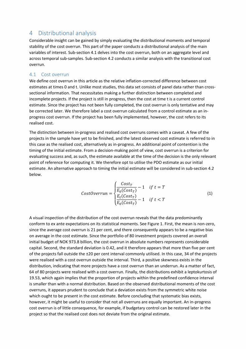
Figure 6: Narrowing of confidence interval Sub-figure (a) presents the development of cost estimate uncertainty proposed by theory. Each dot denotes a new current control estimate, and the vertical lines show the confidence interval associated with the point estimates. According to the literature, the confidence interval should be narrowing as the project is executed. Sub-figure (b) presents the predicted behaviour of the transitional cost overrun on the assumption that the fully efficient estimates are truthfully revealed when the risk is uniformly distributed.

(a)

(b)

5 Regression results In this section, we conduct a formal regression analysis to investigate the statistical relationship

between cost overruns and our selection of independent variables. We start by carrying out an

unvariate panel data regression analysis of common (5.1) and specific project factors (5.2) to

investigate how each individual variable relates to cost overruns. This is followed up in sub-section

5.3 by a multivariate analysis where both total and individual contributions of the independent

variables are analysed jointly.

5.1 Common factors Various case studies performed with offshore petroleum projects on the NCS have led to a

hypothesis that the extent of the cost overruns incurred is driven at least partly by the business cycle.

The proposed relationship between economic activity and cost overruns could reflect a variety of

reasons. First, the cost of input factors and the growth in prices probably change with the business

cycle – in other words, input factors tend to cost less when overall economic activity in the sector is

low, and price inflation also slows. Second, it could be that bargaining power between the operator

and sub-contractors tends to change during booms and busts. Third, access to bottleneck resources

could become more restricted at times when the level of economic activity is high, so that delays –

and by extension cost overruns – occur more frequently. Finally, the business cycle could have an

impact on the effort and scrutiny devoted by project managements to estimating the cost of

potential projects. While several possible proxies are available for the level of economic activity, this

paper will consider oil prices, gas prices, investment on the NCS, employees in the sector and rig

rates.

Inspecting oil prices reveals a relationship between them and cost overruns (see Figure 7). This

relationship is positive, as expected, thereby indicating that overruns tend to be larger when

economic activity is high. While the oil price coefficient is indeed significant, however, its explanatory

power is limited to five per cent. Given that overruns essentially represent unexpected costs, it

seems reasonable to expect that increased oil prices matter to the extent they are not expected. In

line with this idea, it appears that the oil price surprise – the unexpected relative change in oil prices

from following a random walk – may offer a greater explanatory power of seven per cent. This

assumes that companies base their forecasts on a random walk model for oil prices – but it is not

known whether they actually use this approach. If they do not, the explanatory power of an oil price

surprise would probably increase were the company’s actual forecasting model known. Repeating

this exercise with gas prices yields no significant results. The vast majority of the projects considered

in this paper involved facilities on the NCS predominantly producing oil. This may explain the weak

significance of gas prices.

As with oil prices, the level of offshore investment on the NCS proves to have a positive and

significant relationship to cost overruns in petroleum projects (see Figure 8). Furthermore,

unexpected change in sector investment matters more than its absolute level. The causes of this

relationship are a matter of speculation, but one possibility has to do with optimism. When activity is

high, companies have more positive expectations and tend to extrapolate trends, while they are

more pessimistic during downturns and subject their projects to greater scrutiny. Another possibility

is that input prices and capital costs grow faster when economic activity is high. The R2 of sector

investment surprise is considerable, with almost 25 per cent of the cost overruns incurred

explainable by this variable. As its designation implies, investment surprise is not known ex ante the

decision to undertake a project. Were a better method of forecasting investment activity on the NCS

to be developed, however, more of the cost overrun could probably be predicted.

Furthermore, both the sector employee and rig rate variables behave in a similar way to sector

investment. In other words, a positive and significant relationship exists, and the surprise variable

performs better than its respective variables in levels. The sector employee variable also performs

better then sector investment, while rig rates perform less well. Where the employee variable is

concerned, its relationship with cost overrun may reflect higher levels of pay or difficulties in

recruiting workers with key expertise when economic activity is buoyant. A consequent bottleneck in

boom times may cause delays and thereby cost overruns. The rig rate variable has a simpler

explanation – it represents a project cost, and the positive relationship between the rig rate surprise

and cost overruns implies that these units have turned out to be more costly than expected.

Figure 7: Relationship between cost overrun and petroleum prices (a) Oil prices (b) Oil price surprise

(c) Gas prices (d) Gas price surprise

(e) Univariate regression output

Variable Coefficient SE t value p value R2

OilPrice 0.0037 0.0011 3.36 0.0008 0.05 OilPriceSur 0.37 0.06 6.17 6.72 ∗ 10−10 0.07 GasPrice −0.0038 0.0049 −0.78 0.44 0.0018 GasPriceSur −0.13 0.18 −0.70 0.48 0.01

-10

12

3

Co

st ove

rrun

20 40 60 80 100Oil price

beta = .0036 (p-value = 0)

-10

12

3

Co

st ove

rrun

-.5 0 .5 1 1.5 2Oil price surprise

beta = .3398 (p-value = 0)

-10

12

3

Co

st ove

rrun

10 20 30 40 50Gas price

beta = -.0018 (p-value = .591)

-10

12

3

Co

st ove

rrun

-.5 0 .5 1 1.5Gas price surprise

beta = -.139 (p-value = .25)

Figure 8: Relationship between cost overrun and economic activity (a) Sector investment (b) Sector investment surprise

(c) Sector employees (d) Sector employee surprise

(e) Sector rig rates (f) Sector rig rate surprise

(g) Univariate regression output


SecInvest 2.95 ∗ 10−6 1.02 ∗ 10−6 2.54 0.01 0.04 SecInvestSur 0.91 0.20 4.48 4.65 ∗ 10−6 0.24 SecEmp 1.54 ∗ 10−5 5.27 ∗ 10−5 2.93 0.0034 0.07 SecEmpSur 1.79 0.37 4.79 1.65 ∗ 10−6 0.29 RigRates 1.11 ∗ 10−5 3.65 ∗ 10−6 3.04 0.0024 0.05 RigRateSur 0.19 0.03 6.29 3.22 ∗ 10−10 0.10

-10

12

3

Co

st ove

rrun

50000 100000 150000 200000Sector investment

beta = 0 (p-value = .009)

-10

12

3

Co

st ove

rrun

-.5 0 .5 1Sector investment surprise

beta = 1.0194 (p-value = 0)

-10

12

3

Co

st ove

rrun

20000 30000 40000 50000 60000Sector employee


-10

12

3

Co

st ove

rrun

0 .1 .2 .3 .4 .5 Sector employee surprise

beta = 1.9455 (p-value = 0)

-10

12

3

Co

st ove

rrun

0 10000 20000 30000 40000Rig rates


-10

12

3

Co

st ove

rrun

0 1 2 3 4 5 Rig rate surprise

beta = .1734 (p-value = 0)

5.2 Project specific factors We consider the following regressors from the list of idiosyncratic variables: geographic location,

various proxies for complexity (such as ocean depth, execution time, drilling depth and reserve

volume), ownership characteristics (number of rights owners, ownership concentration and operator

experience) and different proxies for project size.

All the projects considered in this paper are located on the NCS. According to the NPD, the NCS is

almost three time the size of mainland Norway and covers 2 039 951 square kilometres. Since

environmental factors, ocean currents, weather and distance from infrastructure can vary

significantly over such a large area, it might prove useful to disaggregate even further geographically.

Applying the categories utilised by the NPD, we disaggregate the NCS into (the Norwegian sector of)

the North Sea, the Norwegian Sea (NoS) and the Barents Sea. Furthermore, we subdivide the

Norwegian North Sea into northern (NNS), central (CNS) and southern (SNS) areas. However, this

regional categorisation yields minuscule results when applied to the scatter plot (see Figure 9). No

discernible difference appears to exist between cost overruns in the different regions. A more formal

approach utilising a univariate regression analysis with dummy variables for the regions described

reveals that only the SNS is marginally significant. Since this area yields a positive coefficient, it would

appear that cost overruns incurred tend to be comparatively larger in the SNS than in other NCS

regions. The SNS is widely regarded as the most mature area of the NCS, with a well-know geology

and short distance to infrastructure. So it seems puzzling that this area should suffer more

substantial cost overruns. As Figure 9 shows, two outliers showing cost overruns exceeding 200 per

cent appear to be associated with the SNS. A priori, this could be the driver of the significant effect

exhibited by the SNS. However, omitting these two observations does not reduce the effect to

insignificance. It is possible that this result is the result of omitted variable bias. For instance, the SNS

has a negative correlation with experience (−0.26) and a positive relationship with realised project

size (0.12). It is consequently possible that this area reflects the fact that projects there tend to be

larger and operated by less experienced companies.

Figure 9: Cost overruns over time by geographic location

-10

12

3

Co

st O

ve

rrun

2000 2005 2010 2015

Southern North Sea (SNS) Central North Sea (CNS)

Northern North Sea (NNS) Norwegian Sea (NoS)

Barents Sea (BS)

Table 10: Univariate regression output


SNS 0.28 0.16 1.77 0.08 0.12

CNS -0.11 0.07 -1.58 0.11 0.02

NNS -0.09 0.06 -1.45 0.15 0.02

NoS -0.06 0.06 -1.05 0.3 0.01

BS 0.12 0.08 1.52 0.13 0

From both theoretical and empirical perspectives, project complexity is expected to provide

significant explanatory power for the cost overrun. As established in section 2, this can be

disaggregated into technical and organisational complexities, which do not necessarily conform in

either effect or significance. Owing to restrictions in data availability, however, only technical

complexity is addressed here. This could potentially be described in numerous ways, but ocean

depth, execution time, drilling depth and reserve volume are utilised in this paper. Contrary to

previous findings, it appears that complexity tends to be orthogonal to cost overruns. According to

Figure 10, all the variables except execution time show an insignificant relationship. If the

fundamental driver of the cost overrun is not the absolute level of complexity but an unexpected

change in complexity, the results can easily be explained. These measures of complexity involve little

surprise – the companies tend to not be taken unawares by ocean depth, for example (there may

however be elements of surprise in complexity factors not covered by our dataset). Furthermore,

execution time appear to be the only variable which yields a significant observed relationship. A rise

in execution time empirically tends to increase the cost overrun. Unlike the previous variables,

execution time influences complexity more indirectly in the sense that complex projects tend to take

longer. So a long project does not necessarily need to be complex. Execution time is frequently used

as a variable in the literature, arguably because of its independence from the specific context. While

ocean depth is a variable with little relevance outside the offshore sector, execution time is relevant

in most cases. However, it involves an inherent complication in that it is an aggregate of planed time

and schedule overrun. Given that delays tend to covariate strongly with cost overruns, it is not

possible to determine whether the delays or the long project time in itself are the true determinant

of the cost overrun.

Arguably, just as project aspects are essential for the prevalence of cost overruns, so the

characteristics of the company responsible for executing the project are probably central to the issue

of cost overrun. To gain an insight into this aspect, we have analysed project ownership and the

responsible operator. Figure 11 shows that neither the number of rights owners nor the

concentration of ownership have any significant effect on a cost overrun. It therefore seems

reasonable to conclude that the experience and skill set possessed by non-operator rights owners

confer minuscule benefits. On the other hand, the experience of the operator appears to have a

significant relationship to cost overruns. The negative coefficient between experience and cost

overruns indicates that more experienced companies tend to suffer fewer/smaller cost overruns then

less experienced operators, even though – as the scatter plot indicates, the effect seems to be

declining. In other words, the benefit conferred by greater experience appears to be getting

marginally smaller. Experience matters a lot initially, but less for each incremental increase in this

variable.

Figure 10: Relationship between cost overrun and technical complexity (a) Ocean depth (b) Execution time

(c) Drilling depth (d) Reserve volume



Execution 0.12 0.04 2.80 0.005 0.1930 OceanDepth -0.0002 0.0002 -1.16 0.24 0.02 DrillingDepth -8.68∗ 10−6 3.37∗ 10−5 -0.26 0.80 0.0016

ReservVol 6.09E-05 0.0002 0.35 0.73 0.0010

-10

12

3

Co

st ove

rrun

0 500 1000 1500Ocean depth

beta = -.0003 (p-value = .045)

-10

12

3

Co

st ove

rrun

0 2 4 6 8Execution time

beta = .1356 (p-value = 0)

-10

12

3

Co

st ove

rrun

1000 2000 3000 4000 5000 6000Drilling depth


-10

12

3

Co

st ove

rrun

0 500 1000 1500Reserve volume

beta = .0001 (p-value = .55)

Figure 11: Operator and ownership characteristics (a) Rights owners (b) Ownership concentration

(c) Experience

(d) Univariate regression output


RightsOwners −0.04 0.03 −1.10 0.27 0.02 OwnCon −0.10 0.11 −0.88 0.38 0.01 Exp −0.0004 0.0002 −2.73 0.01 0.02

As noted in section 2, disagreement prevails in the literature over the kind of relationship which

exists between project size and cost overrun. As can be seen from Figure 12 (b), however, this

particular data sample presents a significant positive relationship between these variables. It would

consequently appear that larger projects tend to be more difficult to estimate. Looking further into

the problem of the conflicting research findings, one proposed reason is that the choice of proxy for

project size is not irrelevant to the results obtained. In other words, defining project size in terms of

the initial ex ante estimate or of the realised ex post cost could yield different values for the beta

coefficient. This possibility can easily be tested. Figures 12 (a) and (b) appear to show that the

fundamental behaviour of both proxies conforms to each other, but a formal regression analysis

reveals that their respective coefficients differ. While both are positive, using the initial estimate

yields a non-significant beta value while the realised cost results in a significant relationship. To see

why this happens, consider 12 (c) where we plot initial estimate against the realised cost. As can be

seen, a non-perfect relationship exists between these proxies in the sense that the correlation is not

equal to one. This implies that, if the portfolio of projects considered in this paper were to be ranked

by size, a distortion would arise from using different measures of project size. As the distortion

increases and thereby reduces the correlation, the difference between the two beta coefficients is

-10

12

3

Co

st ove

rrun

0 2 4 6 8 10Rights owners

beta = -.0476 (p-value = .047)

-10

12

3

Co

st ove

rrun

.2 .4 .6 .8Ownership concentration

beta = .0192 (p-value = .923)

-10

12

3

Co

st ove

rrun

0 100 200 300 400 500Experience

beta = -.0006 (p-value = 0)

expected to continue rising. It would thereby appear that the lack of a prevailing consensus has been

at least partly explained.

Leaving aside the imperfect correlation, a closer analysis of the scatter plot depicted in Figures 12 (a)

and (b) shows what appear to be two distinct regimes in the data. In the lower interval, the inherent

volatility appears to be considerably larger than in the higher interval. An interesting consequence of

this property is that, even though cost overruns empirically tend to increase with project size, the

heteroscedasticity of the data means that the largest anecdotal cost overrun cases are confined to

the lower end of the size scale. This could be explicable in terms of portfolio theory. If we regard a

large project as a portfolio consisting of several independent smaller projects, it is effectively

eliminating idiosyncratic risk through diversification. Small projects are thereby more exposed to risk

than diversified larger projects, which means they exhibit greater volatility than the latter. Given

these characteristics of project size, it would be interesting to verify if the relationship between cost

overrun and the two regimes differs. To investigate this, two clusters are defined so that the

boundary between them is a vertical vector and the sum of the squared distance of each observation

to its cluster centroid is minimised. Figure 12 (d) presents this sub-division of the data. As seen in

Figure 12 (f), the coefficients obtained differ in coefficient, significance and explanatory power.

Unfortunately, neither is capable of producing any significant relationship. There may simply not be

enough data to support a disaggregation on this scale because the sub-sample becomes too small.

Figure 12: Relationship between cost overrun and project size (a) Project investment start (b) Project investment end

(c) Comparison between start and end (d) Cluster analysis of project investment end



MegaPro 0.13 0.12 1.07 0.29 0.03 ProInvestStart 2.60 ∗ 10−6 1.65 ∗ 10−6 1.58 0.11 0.01 ProInvestEnd 2.45 ∗ 10−6 1.35 ∗ 10−6 1.82 0.07 0.02 Cluster 1 (small) 1.76 ∗ 10−5 1.26 ∗ 10−5 1.39 0.164 0.1127 Cluster 2 (high) 6.21 ∗ 10−7 8.72 ∗ 10−7 0.71 0.476 0.0005

-10

12

3

Co

st ove

rrun

0 20000 40000 60000 80000Project investment start


-10

12

3

Co

st ove

rrun

0 50000 100000 150000Project investment end


0

20

00

040

00

060

00

080

00

0

Pro

ject in

ve

stm

ent sta

rt


Corr = .9615

-10

12

3

Co

st ove

rrun


5.3 Multivariate regression analysis While a univariate regression can yield worthwhile insights into cost overruns, a more rigorous

multivariate analysis is essential for gaining further understanding. Given a limited number of

observations and a comparably large set of explanatory variables, many of them highly correlated,

the most suitable scheme for variable inclusion is forward selection. In other words, the model

moves from parsimony to complexity by incrementally including the variable which makes the

greatest contribution to the explanatory power of the model. The process is terminated when the

next inclusion yields an insignificant regressor. In addition to the independent variables listed

previously, several of these are considered with non-linear transformations. Adopting this

methodology, a model with four variables yields an R2 of almost 45 per cent. See Table 11 for further

details.

Table 11: Multivariate model results This table displays the regression output from a model with cost overrun as the dependent variable and four independent variables. The explanatory variables are (1) the sector employee surprise (SecEmpSur), calculated as the relative difference between the number of employees on the NCS today and at the time of the decision, (2) the transitional cost overrun (TraCO) between two subsequent periods, (3) the inverse of the project’s realised investment size (ProInvestEndInv) in NOK, and (4) the operator’s experience in terms of the number of licences it holds.

Regressor Coefficient t-value p-value Own R2 Cumulative R2

SecEmpSur 1.77 3.29 0 0.2938 0.2938

TraCO 0.8 6.28 0 0.2676 0.4189

ProInvestEndInv -188.91 -1.66 0.1 0.0627 0.4456

log(exp) -0.06 -2.22 0.03 0.0535 0.4467

Note: random effect panel data with cluster and heteroscedastic robust standard errors

First, the variable among the four identified with the greatest explanatory power is the sector

employee surprise (SecEmpSur). It exposes a strong connection between cost overrun and business

cycle. Furthermore, this variable shows that what matters is not the absolute level of economic

activity, but the unexpected change in it. In line with ex ante expectations, a positive relationship

exists between SecEmpSur and the cost overrun. It thereby appears that cost overruns tends to rise

when economic activity increases beyond its level at the time the decision to execute the project was

taken. Second, the lagged transitional cost overrun has the second strongest explanatory power in

the model identified. As shown in section 4.2, a high degree of persistence, and even of significant

upward momentum, exists between each incremental updated estimate in the transitional cost

overrun throughout the project execution phase. The implications of this finding are clear. If a project

has experienced a cost overrun in one execution period, it is likely to incur an even higher cost overrun

in the next. It is this persistence and momentum in the transitional cost overrun which makes it a

good predictor of in-progress and realised cost overruns. Third, the inverse of the actual project

investment has substantially weaker explanatory power than the two preceding variables. In line with

the prevailing consensus in the literature, a positive relationship – albeit weak – exists between the

project’s investment size and the cost overrun. However, this finding comes with one caveat. While

the cost overrun appears to trend upwards as investment size increases, variability appears to

decrease. This causes the data to show a funnel shape. Projects with the greatest cost overrun are

consequently located in the lowest size echelons. In other words, caution should be exercised when

recommending policy on the basis of the relationship identified between size and cost overrun.

Finally, experience provides the lowest explanatory power of the four variables identified. The results

show that project operators with greater experience in terms of the number of operatorships they hold on

the NCS tend to have less cost overrun, ceteris paribus, than other, less experienced operators.

External validity is an essential question in any empirical study, which makes it essential to perform

robustness checks of the regression results as far as possible. To address the validity of the

significance found for the coefficient estimates obtained in Table 11, we have constructed an

empirical distribution for the regressors by bootstrapping. As Table 12 shows, the standard errors

change slightly but not by so much that the conclusion on the level of significance are altered. This

corroborating evidence strengthens our confidence in the findings.

Table 12: Robustness check of multivariate model results This table presents a robustness check of the results obtained from the multivariate model described in Table 11 by bootstrapping the standard errors used for the subsequent hypothesis testing.

Regressor Coefficient Std error z p-value 95% Conf. Interval

SecEmpSur 1.77 0.35 5.01 0 1.08 2.46

TraCO 0.8 0.36 2.22 0.03 0.09 1.5

ProInvestEndInv -188.91 86.15 -2.19 0.03 -357.77 -20.06

log(exp) -0.06 0.01 -4.37 0 -0.09 -0.04

6 Discussion The essential problem posed by deviations from estimated investment costs is not their existence,

but the particular distributional form exhibited – in other words, the peculiarity of a positive mean

and positive skewness. After all, random error would always ensure at least a symmetric distribution

around zero. The presence of a skewed distribution centred above zero is arguably of greater

concern, since it implies a bias in the ex ante cost estimate.

In Flyvbjerg’s seminal work, the observed deviation from symmetric white noise is explained by the

mechanisms of cognitive bias and intentional deception. However, this theory was coined in the

context of public-sector projects, and it is more dubious whether the deception hypothesis applies to

the same extent in the private sector with its different incentives. Unlike the case with governments,

no taxpayers exist to finance an economically unsound project. In other words, the discipline

imposed by the threat of bankruptcy means that decision-making based on empire-building and

misguided altruism should be far less prevalent. While the incentive to deceive appears at a first

glance to be lacking in the private sector, however, the predicted distributional skewness

nevertheless persists. One reason may be that different divisions or subsidiaries of a company

compete for scarce investment funds, and that they may have a strategic incentive to underreport

expected investment cost. This is possible in a realistic setting of asymmetric information.

Arguably, one of the shortcomings of inferring the underlying cost overrun driver purely from the

distribution is that this is exposed to the classic problem of underdetermination – the presence of

positive skewness could be caused by several factors which cannot be distinguished from each other.

To underline the point, three of the four categories of cost overrun theories – psychological,

economic and political – are not observable. While cognitive bias and deception might not be directly

observable, technical explanations are. Instead of making inferences about the cost overrun driver on

the basis of the unconditional distribution of the cost overrun, it would be more insightful to look at

the conditional distribution after netting out the effects of observable technical drivers. If the

theoretical categorisation really is mutually exclusive and collectively encompassing, the residual cost

overrun after controlling for the technical aspect must be caused by these unobservable

explanations.

The regression model derived in the preceding section with an explanatory power of 44.67 per cent –

arguably impressive considering the oxymoronic task of predicting unpredicted costs – is a good

point of departure for removing the effect of technical drivers from the cost overrun. As shown in

Figure 13 and Table 13, after conditioning the cost overrun distribution with the insight gained from

the multivariate model, the residual cost overrun shifts towards zero but the inherent skewness

proves to be more resilient. While the average cost overrun moves from 21 to zero per cent, the

skewness merely shifts from 3.60 to 2.98. Despite our best efforts, technical explanations are unable

to account satisfactorily for the observed skewness, and we therefore find the deception hypothesis

to be more likely. However, this conclusion relies on the notion that no alternative mechanism exists

which can provide skewness.

Table 13: Statistical movements of the cost overrun distribution

Variable Mean Std dev Min Median Max Skew Kurt

Cost overrun 0.21 0.43 −0.72 0.09 2.93 3.6 19.53

Predicted 0.3 0.3 −0.48 0.23 1.54 0.76 4.71

Residual 0.01 0.38 −0.5 −0.05 1.9 2.98 13.91

Figure 13: Comparison between unconditional and conditional cost overrun distributions

A commonly overlooked problem in research on cost overruns is that these can only occur if a project

is undertaken. This point might appear self-evident, but arguably has some profound effects. If

the investment opportunity portfolio exceeds the company’s capital constraint, it is forced to set

priorities. Should the company make biased estimates for all opportunities, the bias will not be

detected unless the company undertakes the particular project. To see why this is problematic,

consider the following. Even when the estimates are on average unbiased and symmetric, the

realised cost overrun distribution will still be biased and skewed simply because the company is

actively opting for the most profitable projects. All other things being equal, a project with a negative

cost-estimate bias will appear more profitable than a project with a positive one. Projects with

negative cost bias will yield a cost overrun by definition, which explains the observed positive mean

and skewness in the cost overrun distribution. This alternative explanation might have some merits,

but the strength of the mechanism is unclear. A conservative guess might be that this sample

selection bias is significant but limited. Based on the sheer amount of skewness and average cost

overrun observed in the unconditional distribution, it is doubtful that sample selection bias can

explain it all. In light of the conditional distribution, however, since most of the average cost overrun

dissipates, the sample selection hypothesis has become more probable. In any event, whether

cognitive bias, deception, sample selection bias or some unobserved technical aspect represents the

01

23

De

nsity


Unconditional Conditional

true driver of the residual skewness in the cost overrun, this cannot be determined on the basis of

the available data and thus remains a conundrum to be addressed by further research.

Figure 14: Cost estimating distorted by white noise This figure illustrates the actual cost of a project distorted by symmetric white noise. For a given project, a negative bias will (ceteris paribus) cause the NPV of the project to increase and consequently produce a cost overrun if the project is undertaken. Similarly, a positive bias will decrease the estimated NPV and give rise to cost underruns if the projects is realised.

7 Conclusion Through an extensive analysis based on econometrics, this paper has addressed both the prevalence

and the underlying drivers of cost overruns in petroleum projects on the NCS. As noted throughout

this paper, such cost overruns are a common phenomenon but not drastically different from those

experienced in public infrastructure projects. A significant proportion of the cost overrun can be

explained through regression analysis. Among the prominent findings, cost overruns are significantly

linked to unexpected changes in the level of economic activity, but not particularly driven by

technical complexity. It is the combination of these two findings which leads us to conclude that cost

overruns are driven by the element of surprise. Inspection of transitional cost overruns – the relative

change between two consecutive cost estimates – shows a deviation from efficient information

updating. More research is required to establish whether this is because of a lack of effort or

intentional deception. Despite the available data and our best efforts, the residual unexplained cost

overrun exhibits positive skewness. More research is therefore clearly required to gain a complete

understanding of the dynamics of cost overruns.

Cost overruns raise a number of issues that we have not been able to address in the current paper,

due to limitations in the data set. These are topics for future research. One of these is exchange rate

effects. The budgets we analyse are in NOK, whereas the costs are in different currencies. The cost

overruns should therefore be adjusted with exchange rate changes. For instance, NOK has

depreciated towards USD and Euro since 2011/2012. This increases the cost in NOK for imports and

thus inflates the cost overrun.

The paper is analysing a period with close to continuous growth in the petroleum investments. The

times have now changed and we see cost underruns in several projects. Ideally, we would have liked

a data set containing several business cycles. At this period of high oil price oil companies have

prioritised high production volumes and early start of production, even if this led to higher cost. In a

high oil price regime this can be a good trade-off.

Project complexity is expected to provide significant explanatory power for cost overrun. Testing for

sea depth and drilling depth, we are unable to confirm this, probably because there are no elements

of surprise in these factors. Other factors generating complexity that would be useful to consider, are

the choice of development concept (subsea, jacket, floater, etc.), the experience of the suppliers in

delivering according to Norwegian standards, geology, reservoir characteristics (fragmented

reservoir, high pressure and high temperature), oil quality (heavy oil), and new technology.

Bibliography Altshuler, A. A. and D. Luberoff (2003). Mega-projects: The changing politics of urban public

investment. Brookings Institution Press.

Arvan, L. and A. P. Leite (1990). Cost overruns in long term projects. International Journal of

Industrial Organization 8 (3), 443–467.

Baccarini, D. (1996). The concept of project complexity—a review. International Journal of Project

Management 14 (4), 201–204.

Bertisen, J. and G. A. Davis (2008). Bias and error in mine project capital cost estimation. The

Engineering Economist 53 (2), 118–139.

Bordat, C., B. McCullouch, and K. Sinha (2004). An analysis of cost overruns and time delays of indot

projects. Joint Transportation Research Program, 11.

Bosch-Rekveldt, M. and H. Mooi (2008). Research into project complexity classification methods.

IPMA World Congress 22 (2), 104–109.

Bruzelius, N., B. Flyvbjerg, and W. Rothengatter (2002). Big decisions, big risks. improving

accountability in mega projects. Transport Policy 9 (2), 143–154.

Buehler, R., D. Griffin, and M. Ross (1994). Exploring the” planning fallacy”: Why people

underestimate their task completion times. Journal of personality and social psychology 67 (3), 366.

Cantarelli, C. C. (2011). Cost Overruns in Large-Scale Transport Infrastructure Projects: A theoretical

and empirical exploration for the Netherlands and worldwide. TU Delft, Delft University of

Technology.

Cantarelli, C. C., B. Flyvbjerg, E. J. Molin, and B. Van Wee (2010). Cost overruns in large-scale

transportation infrastructure projects: explanations and their theoretical embeddedness. European

Journal of Transport Infrastructure Research 10 (1), 5–18.

Creedy, G. D. (2006). Risk factors leading to cost overrun in the delivery of highway construction

projects.

Dantata, N. A., A. Touran, and D. C. Schneck (2006). Trends in us rail transit project cost overrun.

Transportation Research Board.

Eliasson, J. and M. Fosgerau (2013). Cost overruns and demand shortfalls–deception or selection?

Transportation Research Part B: Methodological 57, 105–113.

Flyvbjerg, B. (2008). Curbing optimism bias and strategic misrepresentation in planning: Reference

class forecasting in practice. European Planning Studies 16 (1), 3–21.

Flyvbjerg, B., N. Bruzelius, and W. Rothengatter (2003). Megaprojects and risk: An anatomy of

ambition. Cambridge University Press.

Flyvbjerg, B., M. S. Holm, and S. Buhl (2002). Underestimating costs in public works projects: Error or

lie? Journal of the American planning association 68 (3), 279–295.

Flyvbjerg, B., M. K. Skamris Holm, and S. L. Buhl (2003). How common and how large are cost

overruns in transport infrastructure projects? Transport reviews 23 (1), 71–88.

Flyvbjerg, B., M. K. Skamris Holm, and S. L. Buhl (2004). What causes cost overrun in transport

infrastructure projects? Transport reviews 24 (1), 3–18.

Flyvbjerg, B. and A. Stewart (2012). Olympic proportions: Cost and cost overrun at the olympics 1960-

2012.

Fouracre, P., R. J. Allport, and J. Thomson (1990). The performance and impact of rail mass transit in

developing countries. Technical report.

Gil, N. and C. Lundrigan (2012). The leadership and governance of megaprojects. Technical report,

CID Technical Report.

Gray, A. R., S. G. MacDonell, and M. J. Shepperd (1999). Factors systematically associated with errors

in subjective estimates of software development effort: the stability of expert judgment. In Software

Metrics Symposium, 1999. Proceedings. Sixth International, pp. 216–227. IEEE.

Grieco, D. and R. M. Hogarth (2009). Overconfidence in absolute and relative performance: The

regression hypothesis and bayesian updating. Journal of Economic Psychology 30 (5), 756–771.

Hall, P. G. (1982). Great planning disasters, Volume 1. Univ of California Press. Hatton, L. (2007). How

accurately do engineers predict software maintenance tasks? Computer (2), 64–69.

Heemstra, F. and R. Kusters (1991). Function point analysis: Evaluation of a software cost estimation

model. European Journal of Information Systems 1 (4), 229–237.

Hill, J., L. Thomas, and D. Allen (2000). Experts’ estimates of task durations in software development

projects. International journal of project management 18 (1), 13–21.

Jørgensen, M. (2013). The influence of selection bias on effort overruns in software development

projects. Information and Software Technology 55 (9), 1640–1650.

Jørgensen, M., T. Halkjelsvik, and B. Kitchenham (2012). How does project size affect cost estimation

error? statistical artifacts and methodological challenges. International Journal of Project

Management 30 (7), 839–849.

Kahneman, D. and D. Lovallo (1993). Timid choices and bold forecasts: A cognitive perspective on risk

taking. Management science 39 (1), 17–31.

Kahneman, D. and A. Tversky (1977). Intuitive prediction: Biases and corrective procedures. Technical

report, DTIC Document.

Kahneman, D. and A. Tversky (1979). Prospect theory: An analysis of decision under risk.

Econometrica: Journal of the Econometric Society, 263–291.

Kruger, J. and D. Dunning (1999). Unskilled and unaware of it: how difficulties in recognizing one’s

own incompetence lead to inflated self-assessments. Journal of personality and social psychology 77

(6), 1121.

Lee, J.-K. (2008). Cost overrun and cause in Korean social overhead capital projects: Roads, rails,

airports, and ports. Journal of Urban Planning and Development 134 (2), 59–62.

Love, P. E., D. J. Edwards, and Z. Irani (2012). Moving beyond optimism bias and strategic

misrepresentation: An explanation for social infrastructure project cost overruns. Engineering

Management, IEEE Transactions on 59 (4), 560–571.

Love, P. E., D. J. Edwards, and J. Smith (2005). Contract documentation and the incidence of rework

in projects. Architectural Engineering and Design Management 1 (4), 247–259.

Mackie, P. and J. Preston (1998). Twenty-one sources of error and bias in transport project appraisal.

Transport policy 5 (1), 1–7.

Mansfield, N. R., O. Ugwu, and T. Doran (1994). Causes of delay and cost overruns in nigerian

construction projects. International Journal of Project Management 12 (4), 254–260.

McKenna, M. G., H. Wilczynski, and D. VanderSchee (2006). Capital project execution in the oil and

gas industry. Booz Allen Hamilton, Houston.

Moløkken-Østvold, K., M. Jørgensen, S. S. Tanilkan, H. Gallis, A. C. Lien, and S. E. Hove (2004). A

survey on software estimation in the norwegian industry. In Software Metrics, 2004. Proceedings.

10th International Symposium on, pp. 208–219. IEEE.

Morris, P. W. and G. H. Hough (1987). The anatomy of major projects: A study of the reality of project

management.

Nijkamp, P. and B. Ubbels (1999). How reliable are estimates of infrastructure costs? a comparative

analysis. International Journal of Transport Economics/Rivista internazionale di economia dei

trasporti, 23–53.

Odeck, J. (2004). Cost overruns in road construction—what are their sizes and determinants?

Transport policy 11 (1), 43–53.

Olawale, Y. A. and M. Sun (2010). Cost and time control of construction projects: inhibiting factors

and mitigating measures in practice. Construction Management and Economics 28 (5), 509–526.

Osmundsen, P., K. H. Roll, and R. Tveter˚as (2010). Exploration drilling productivity at the norwegian

shelf. Journal of Petroleum Science and Engineering 73 (1), 122–128.

Pickrell, D. H. (1989). Urban rail transit projects: forecast versus actual ridership and costs. final

report. Technical report, Transportation Systems Center, Cambridge, MA (USA).

Pickrell, D. H. (1992). A desire named streetcar fantasy and fact in rail transit planning. Journal of the

American Planning Association 58 (2), 158–176.

Remington, K. and J. Pollack (2008). Are there special tools for complex projects. IPMA World

Congress 22 (2), 104–109.

Sandberg, F. H. and P. W. Hetland (2008). Is making decisions just a gut feeling? IPMA World

Congress 22 (2), 940–945. Sauer, C., A. Gemino, and B. H. Reich (2007). The impact of size and

volatility on it project performance. Communications of the ACM 50 (11), 79–84.

Staats, B. R., K. L. Milkman, and C. R. Fox (2012). The team scaling fallacy: Underestimating the

declining efficiency of larger teams. Organizational Behavior and Human Decision Processes 118 (2),

132–142.

Van Oorschot, K., J. Bertrand, and C. G. Rutte (2005). Field studies into the dynamics of product

development tasks. International Journal of Operations & Production Management 25 (8), 720–739.

Wachs, M. (1982). Ethical dilemmas in forecasting for public policy. Public Administration Review,

562–567. Wachs, M. (1987). Forecasts in urban transportation planning: Uses, methods, and

dilemmas. Climatic Change 11 (1-2), 61–80.

Wachs, M. (1990). Ethics and advocacy in forecasting for public policy. Business & professional ethics

journal, 141–157.

Weinstein, N. D. (1980). Unrealistic optimism about future life events. Journal of personality and

social psychology 39 (5), 806.

Yang, D., Q. Wang, M. Li, Y. Yang, K. Ye, and J. Du (2008). A survey on software cost estimation in the

chinese software industry. In Proceedings of the Second ACM-IEEE international symposium on

Empirical software engineering and measurement, pp. 253–262. ACM.

We examine drivers of cost overruns in Norwegian ... - CORE · PDF fileAmong the significant...

Documents

Transcript of We examine drivers of cost overruns in Norwegian ... - CORE · PDF fileAmong the significant...