Verification of SMOM and QMOM Population Balance Modeling in CFD code Using Analytical Solutions for Batch Particulate Processes

Bin Wan and Terry A. Ring Dept. Chemical Engineering University of Utah Salt Lake City, UT 84112

and

Kumar M. Dhanasekharan and Jayanta Sanyal Fluent Inc. 10 Cavendish Court Lebanon, NH 03766

Abstract For many processes of industrial significance, due to the strong coupling between particle interactions and fluid dynamics, the population balance must be solved as part of a computational fluid dynamics (CFD) simulation. In this work, a CFD based population balance model is tested using a batch crystallization reactor. In this CFD model, the population balance is solved by the standard method of moments (SMOM) and the quadrature method of moments (QMOM). The results of these simulations are compared to analytical solutions for the population balance in a batch tank where 1) nucleation 2) growth, 3) aggregation, and 4) breakage are taking place separately. The results of these comparisons show that the first 6 moments of the population balance are accurately predicted for nucleation, growth, aggregation and breakage at all times. Keywords: Population balance; Computational fluid dynamics; Particle process; Modeling

1. Introduction Batch crystallization processes are widely used, especially in the pharmaceutical industry. Batch crystallization processes are not well understood because the process is affected dramatically by fluid mixing, particle aggregation and particle breakage. Simple models used for batch crystallization do not account for mixing, aggregation and breakage. In order to properly model batch crystallization the population balance must be coupled with turbulent computational fluid dynamics (CFD) modeling to correctly predict the particle size distribution (PSD). Such a model has been created based upon either the Sandard Method of Moments (SMOM) or the quadrature method of moments1 (QMOM within a well established CFD model to solve the PSD for industrial problems, such as batch crystallization and batch precipitation. This work describes our attempts to verify this new computer code with analytical solutions

1

to the population balance for batch conditions. Verification is the first step on the road to model validation with experimental data, to be handled in another publication. In this verification work, we compare these CFD results with analytical solutions to the population balance model for a batch crystallizer using nucleation only, growth only, aggregation only, and breakage only cases. The QMOM solution to the population balance is calculated using the first 6 moments (zero to five) of the population. For comparison, the analytical solutions are reduced to the first 6 moments of the population and compare directly with CFD simulation results.

2. Batch Population Balance Equation (PBE) The population balance equation (PBE) is a statement of continuity for particulate systems. For a batch crystallizer with nucleation, aggregation, breakage and growth occurring, the PBE is given by Randolph and Larson 2 as

)()()),()((),( vdvbv

tvnvGt

tvn−=

∂∂

+∂

∂ [1]

with the initial condition, n(v,t=0) = no(v). In the above equation n(v) is the number-based population of particles in the crystallizer which is a function of the particle volume, v. G(v) is the volume dependent growth rate and b(v) is the volume dependent birth rate and d(v) is the volume dependent death rate. For aggregation, the birth and death rate terms are given by Hulburt and Katz 3:

∫∫∞

−−−=−0

2/

0)(),()()()(),()()( duunuvvnduunuvnuuvvdvb

v

aa ββ [2]

where the aggregation rate constant, β(v,w), is a measure of the frequency of collision of particles of size v with those of size u. In the case of breakage, the birth and death rate terms are given by Prasher 4:

)()()(),()()()( vnvSdwwnwvwSvdvbvbb −=− ∫∞

ρ [3]

where S(v) is the breakage rate that is a function of particle size, v, ρ(v,w) is the daughter distribution function defined as the probability that a fragment of a particle of size w will appear at size v. In this paper, we use analytical solutions to the population balance for comparison with standard method of moments (SMOM) and quadrature method of moments (QMOM) CFD solutions to the population balance. With SMOM and QMOM the population balance is simplified into a series of a few discrete moment equations. Certain moments of the population have

2

physical significance as shown in Table 1. The kth volume-based moment is defined by5:

∫∞

=0

)( dvvnvm kkv [4]

vmo and vm1 represent the total number and total volume of particles in the system. In the CFD code, the particle density function is described as a function of particle size x, instead of particle volume v and the population balance is written in terms of n(x) instead of n(v). Thus the population balance, eq. [1], is rewritten as:

)()()),()((),( xdxbx

txnxGt

txn−=

∂∂

+∂

∂ [5]

and the kth length-based moment is defined by6:

∫∞

=0

)( dxxnxm kkL [6]

A comparison of several volume-based moments and length-based moments are given in Table 1. Table 1: Comparison of volume based moments and length-based moments: Property

Volume-Based Moment

Length-Based Moment

Number of Particles

vm0 Lm0

Surface Area of Particles

Kav*vm2/3 Ka*Lm2

Volume of Particles

vm1 Kv*Lm3

Ka, Kav and Kv are area and volume shape factors The SMOM proposed by Randolph and Larson2 is an alternative method for solving the PBE. Instead of solving PBE, equation [1], directly, SMOM converts the PBM into several moment equations that are solved separately. The moment transformation for growth and breakage is given by:

∫∫∞∞

−=∂

∂+

00

),()()12()),()(()(dvtvnvSvdv

vtvnvGv

dttmd i

iiiv η [7]

where ηi is defined as:

3

[8] ξξξη dvPii )'|(

1

0∫=

where P(v|v’) is daughter distribution function, assuming that P(v|v’) is purely a function of ξ=v/v’. The advantages to this approach are that SMOM reduces the dimensionality of the problem significantly. It is relatively simple to solve the transport equations for lower-order moments. The disadvantages are that exact closure of the growth term and the right-hand side of equation [7] is possible only in special cases - those with polynomial breakage rate combined with a daughter distribution that is a polynomial in v/v’, constant aggregation rate and either size-independent growth rate or linear (in volume) growth rate. In all other cases, closure is not possible. Closure is the situation where equation [7] reduces to a set of equations where the equation for d vmi/dt only has terms with equal or lower order moments allowing the solution for all order moments in terms of lower or equal order moments and never higher order moments. This closure constraint is overcome, however, with QMOM. The QMOM method was first proposed by McGraw7 for modeling the size evolution of aerosols and for coagulation problems. Its applications by Marchisio et al.8 have shown that the method requires a relatively small number of scalar equations to track the moments of population with small errors. The QMOM method provides an attractive alternative to the SMOM method for size dependant growth, size dependant aggregation and breakage. Rather than an exact PSD, QMOM gives a series of N weights and N abscissas that can be converted into 2N moments. Its advantages are that there are fewer variables (typically only six moments) and a dynamic calculation of the size bins. The disadvantages are that the number of abscissas may not be adequate to describe the PSD and that solving the Product-Difference algorithm9 may be time consuming. The QMOM method is based on the following quadrature approximation.

∫ ∑∞+

=

≈=0

1

)(N

i

kii

kkL LwdLLLnm [11]

where weights ( ) and abscissas ( ) are determined through the product-difference(PD) algorithm from the lower-order moments

iw iL9; By using the PD

algorithm, a quadrature approximation with N weights and N abscissas can be constructed using the first 2N moments of the PSD. In the CFD simulations presented in this work, N = 3 giving the first six moments (Lm0, Lm1, Lm2, Lm3, Lm4, and Lm5). Using the quadrature approximation,

kkkN

i

kiikL LwLwLwLwm 332211

3

1

++== ∑=

=

[12]

4

any kth moment can be approximated allowing closure of the moment-based population balance equation. The moment-based population balance results in 2N transport equations for the first 2N moments. All these moment transport equations can be solved together with the other transport equations including: the momentum balance and the mass balance equations. In the CFD code, 6 moments are tracked which is enough to characterize the PSD for many cases. For our time dependant well-mixed batch simulations, a single 2D cell is used with CFD code’s multi-phase mixture model. The various parameters for population balance including: nucleation rate, growth rate, aggregation rate and breakage rate can be set to a constant or a user-defined function can be created and compiled within the CFD code. For these simulations the momentum balance and the mass balance were turned off and only the SMOM or QMOM population balance transport equations (PBM) were solved using double precision calculations. The results of these simulations are the first six length-based moments (Lm0, Lm1, Lm2, Lm3, Lm4, and Lm5). These moments are compared directly to those calculated from the analytical solutions of the population balance equation for specific cases discussed in the next section of this paper.

3. Results and Discussion

Case 1 - Nucleation With nucleation the population balance, equation [1], can be simplified by deleting the 2nd and 4th terms. On the right hand side of equation [1] only the birth term for particles of effectively zero size remains. The population balance for this case is given by:

)()(),(oo xxBxb

ttxn

−⋅==∂

∂ δ [13]

where Bo is nucleation rate (#/m3 s), δ(x-xo) is the Dirac delta function centered at the size of the nuclei, xo, with units for the delta function of 1/ µm. Integrating equation [11] with time from the initial condition, n(x,t=0)=0 to t, assuming that the nuclei size xo=0 µm and using the definition of length-based moments, we obtain a solution for the length-based moments:

≠=⋅

=⋅⋅=0,00,

0kktB

tBm okokL . [14]

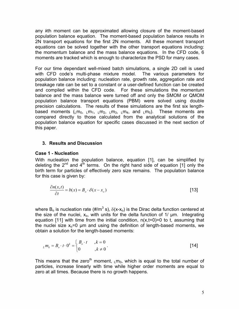
This means that the zeroth moment, Lm0, which is equal to the total number of particles, increase linearly with time while higher order moments are equal to zero at all times. Because there is no growth happens.

5

For the CFD simulations, the nucleation rate was set to Bo = 0.01 #/(m3.µm s) and the convergence criteria was set to 10-4 for every time step. With this convergence criterion it took less than 40 iterations for convergence at each time step. The results for the 0th moment, the total number of particles is shown in Figure 1. Both the SMOM and the QMOM methods in CFD code accurately predict the analytical results given in equation [12] at all times between 0 and 100 s. The higher order moments were also predicted by SMOM and QMOM in CFD code to be zero within round off error for the convergence criterion used in this calculation. Table 2 shows the maximum error in the 0th moment to be 10-6 which is the error associated with the convergence criterion for the calculation.

0

0.2

0.4

0.6

0.8

1

1.2

0 20 40 60 80 1

time (seconds)

00

m0_smmm0_qmomm0_analytical

Figure 1. Comparison of 0th moment values calculated with the analytical solution, eq. [14], SMOM and QMOM methods using CFD code for Case 1 - Nucleation. Table 2. Maximum error for SMOM and QMOM CFD simulations over the time period 0 to 100s for Case 1 – Nucleation Convergence criteria was set to 10-6 for every time step.

Moments Error for SMOM % Error for QMOM % Lm0 10-6 10-6

Case 2 - Growth With growth the population balance, equation [1] is simplified by deleting the

3rd and 4th terms which corresponding to the birth and death terms. In this case we will assume that the growth rate, G(x) [=G] is not a function of particle size, x, and that there is an initial distribution of particles described by a delta function centered at size xm. The population balance for this case is given by:

6

0),(),(=

∂∂

+∂

∂x

txnGt

txn [15]

with initial condition, n(x,t=0) = δ(x-xm). Equation [13] has the analytical solution:

)(),( tGxxtxn m ⋅−−= δ [16]

Using the moments definition, equation [6], and with xm=0, we get,

k

kL tGm )( ⋅= [17] This result states that the total number of particles will not change with time

making the 0th moment is a constant. The higher moments increase with time to a power equal to the order of the moment, for example the 1st moment will increase linearly with time and the second moment will increase quadratically with time, etc. For the CFD simulations, the growth rate was constant at G = 1 µm/s, the initial number of zero sized particles is 100 m-3, which allows the initial conditions for all the moments to be described as:

∫∞

==0

00 100)( dxxnLmL

and 5,4,3,2,1,0)(

0=== ∫

∞ifordxxnLm i

iL

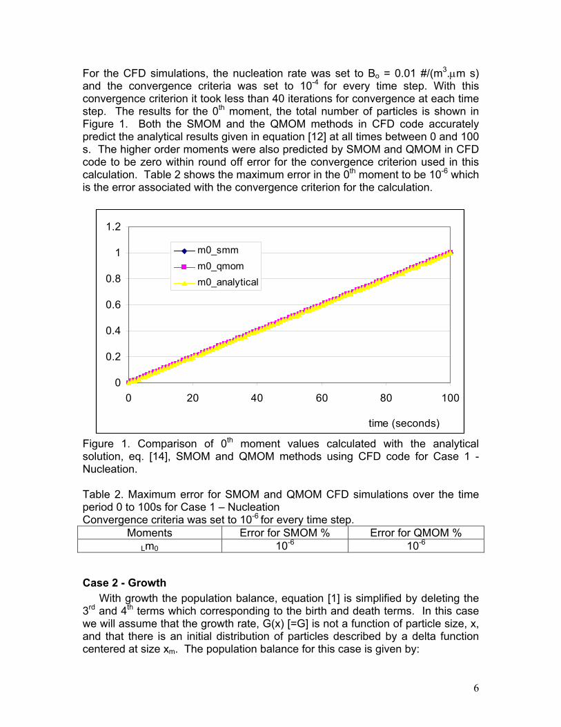
For growth Lm0 is constant with time since the total number of particle does not change but moments 1 to 5 increase with time as the particles grow. Among them, Lm1 will change with time linearly; Lm2 will change quadratically with time, etc. For these CFD calculations, the convergence criteria are set to 10-4 for every time step for both SMOM and QMOM simulations. For this value of the convergence criterion it will took less than 40 iterations for convergence at each time step. The results of the CFD simulations are shown in Figure 2A-F. In Figure 2 we see the values of the various moments plotted as a function of time. In each graph are the SMOM and QMOM simulations as well as the analytical solution given in equation [17]. Both SMOM and QMOM simulations predict the time evolution of the moments reasonably well. The lower moments are predicted accurately but the higher order moments are not predicted as well. Table 3 lists the maximum errors for the various moments over the time period for the simulations shown in Figure 2 as calculated by SMOM and QMOM methods. The maximum errors are worst for the higher moments and approach 10 % for the SMOM CFD simulation while the QMOM simulation is more accurate for showing only 0.7% error.

7

m0 vs. time

0

20

40

60

80

100

120

0 50

time (seconds)

mom

ents

100

m0smm

m0qmom

m0_analytical

A) Lm0

m1 vs. time

0

0.002

0.004

0.006

0.008

0.01

0.012

0 20 40 60 80 100

time (seconds)

mom

ents

m1smm

m1qmom

m1_analytical

B) Lm1

m2 vs. time

0.00E+00

2.00E-07

4.00E-07

6.00E-07

8.00E-07

1.00E-06

1.20E-06

0 50 100

time (seconds)

mom

ents

m2smm

m2qmom

m2_analytical

C) Lm2 D) Lm3

D) Lm4

m5 vs. time

0

2E-19

4E-19

6E-19

8E-19

1E-18

1.2E-18

0 20 40 60 80 100

time (seconds)

mom

ents

m5smm

m5qmom

m5_analytical

F) Lm5

m3 vs. time

0.00E+00

2.00E-11

4.00E-11

6.00E-11

8.00E-11

1.00E-10

1.20E-10

0 50 100

time (seconds)

mom

ents

m3smm

m3qmom

m3_analytical

m4 vs. time

0

2E-15

4E-15

6E-15

8E-15

1E-14

1.2E-14

0 20 40 60 80 100

time (seconds)

mom

ents

m4smm

m4qmom

m4_analytical

Figure 2 Plot of length-based moments 0 to 5 versus time for analytical solution, SMOM and QMOM CFD simulations for Case 2 - Growth.

8

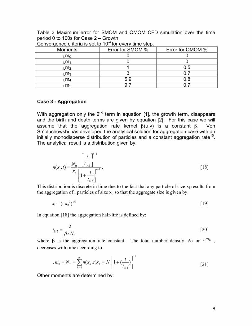
Table 3 Maximum error for SMOM and QMOM CFD simulation over the time period 0 to 100s for Case 2 – Growth Convergence criteria is set to 10-4 for every time step.

Moments Error for SMOM % Error for QMOM % Lm0 0 0 Lm1 0 0 Lm2 1 0.5 Lm3 3 0.7 Lm4 5.9 0.8 Lm5 9.7 0.7

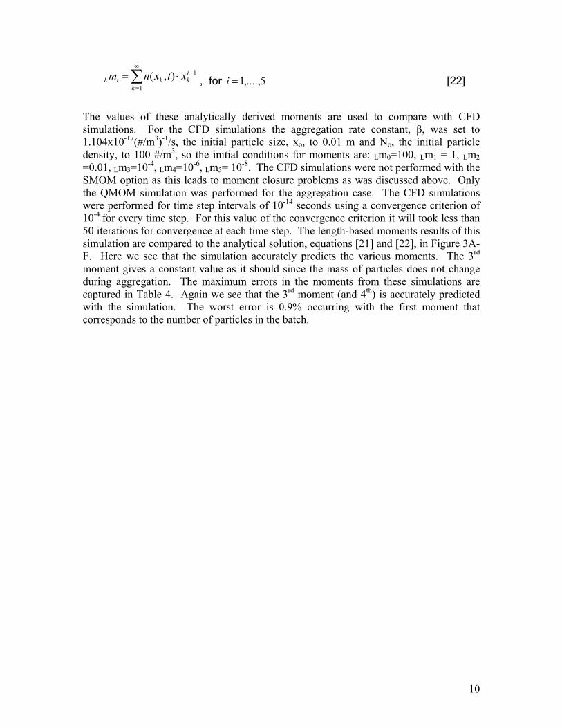
Case 3 - Aggregation With aggregation only the 2nd term in equation [1], the growth term, disappears and the birth and death terms are given by equation [2]. For this case we will assume that the aggregation rate kernel β(u,v) is a constant β. Von Smoluchowshi has developed the analytical solution for aggregation case with an initially monodisperse distribution of particles and a constant aggregation rate10. The analytical result is a distribution given by:

1

2/1

1

2/10

1

),( +

−

+

= i

i

ii

tt

tt

xNtxn . [18]

This distribution is discrete in time due to the fact that any particle of size xi results from the aggregation of i particles of size xo so that the aggregate size is given by: xi = (i xo

3)1/3 [19] In equation [18] the aggregation half-life is defined by:

02/1

2N

t⋅

=β

[20]

where β is the aggregation rate constant. The total number density, NT or , decreases with time according to

0mL

1

2/10

10 )(1),(

−∞

=

+=== ∑ t

tNxtxnNm kk

kTL [21]

Other moments are determined by:

9

1

1

),( +∞

=

⋅= ∑ ik

kkiL xtxnm , for 5,....,1=i [22]

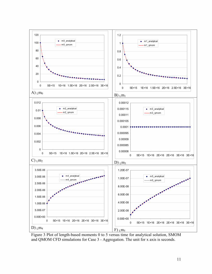
The values of these analytically derived moments are used to compare with CFD simulations. For the CFD simulations the aggregation rate constant, β, was set to 1.104x10-17(#/m3)-1/s, the initial particle size, xo, to 0.01 m and No, the initial particle density, to 100 #/m3, so the initial conditions for moments are: Lm0=100, Lm1 = 1, Lm2 =0.01, Lm3=10-4, Lm4=10-6, Lm5= 10-8. The CFD simulations were not performed with the SMOM option as this leads to moment closure problems as was discussed above. Only the QMOM simulation was performed for the aggregation case. The CFD simulations were performed for time step intervals of 10-14 seconds using a convergence criterion of 10-4 for every time step. For this value of the convergence criterion it will took less than 50 iterations for convergence at each time step. The length-based moments results of this simulation are compared to the analytical solution, equations [21] and [22], in Figure 3A-F. Here we see that the simulation accurately predicts the various moments. The 3rd moment gives a constant value as it should since the mass of particles does not change during aggregation. The maximum errors in the moments from these simulations are captured in Table 4. Again we see that the 3rd moment (and 4th) is accurately predicted with the simulation. The worst error is 0.9% occurring with the first moment that corresponds to the number of particles in the batch.

10

0

20

40

60

80

100

120

0 5E+15 1E+16 1.5E+16 2E+16 2.5E+16 3E+16

m0_analyticalm0_qmom

A) Lm0

0

0.2

0.4

0.6

0.8

1

1.2

0 5E+15 1E+16 1.5E+16 2E+16 2.5E+16 3E+16

m1_analytical

m1_qmom

B) Lm1

0

0.002

0.004

0.006

0.008

0.01

0.012

0 5E+15 1E+16 1.5E+16 2E+16 2.5E+16 3E+16

m2_analytical

m2_qmom

C) Lm2

0.00008

0.000085

0.00009

0.000095

0.0001

0.000105

0.00011

0.000115

0.00012

0 5E+15 1E+16 2E+16 2E+16 3E+16 3E+16

m3_analytical

m3_qmom

D) Lm3

0.00E+00

5.00E-07

1.00E-06

1.50E-06

2.00E-06

2.50E-06

3.00E-06

3.50E-06

0 5E+15 1E+16 2E+16 2E+16 3E+16 3E+16

m4_analytical

m4_qmom

D) Lm4

0.00E+00

2.00E-08

4.00E-08

6.00E-08

8.00E-08

1.00E-07

1.20E-07

0 5E+15 1E+16 2E+16 2E+16 3E+16 3E+16

m5_analytical

m5_qmom

F) Lm5 Figure 3 Plot of length-based moments 0 to 5 versus time for analytical solution, SMOM and QMOM CFD simulations for Case 3 - Aggregation. The unit for x axis is seconds.

11

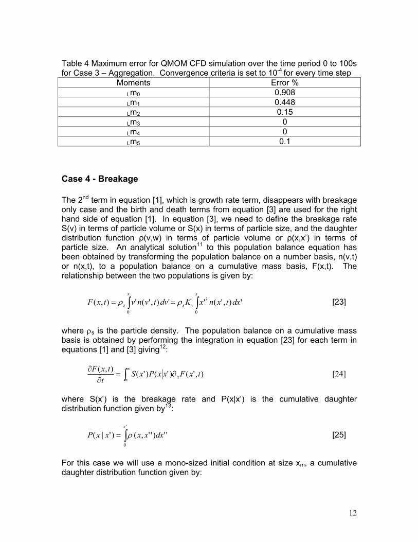
Table 4 Maximum error for QMOM CFD simulation over the time period 0 to 100s for Case 3 – Aggregation. Convergence criteria is set to 10-4 for every time step

Moments Error % Lm0 0.908 Lm1 0.448 Lm2 0.15 Lm3 0 Lm4 0 Lm5 0.1

Case 4 - Breakage The 2nd term in equation [1], which is growth rate term, disappears with breakage only case and the birth and death terms from equation [3] are used for the right hand side of equation [1]. In equation [3], we need to define the breakage rate S(v) in terms of particle volume or S(x) in terms of particle size, and the daughter distribution function ρ(v,w) in terms of particle volume or ρ(x,x’) in terms of particle size. An analytical solution11 to this population balance equation has been obtained by transforming the population balance on a number basis, n(v,t) or n(x,t), to a population balance on a cumulative mass basis, F(x,t). The relationship between the two populations is given by:

[23] '),'(''),'('),(0

3

0

dxtxnxKdvtvnvtxFx

vs

x

s ∫∫ == ρρ

where ρs is the particle density. The population balance on a cumulative mass basis is obtained by performing the integration in equation [23] for each term in equations [1] and [3] giving12:

∫∞

∂=∂

∂x x txFxxPxS

ttxF ),'()'()'(),( [24]

where S(x’) is the breakage rate and P(x|x’) is the cumulative daughter distribution function given by13:

[25] ∫='

0

'')'',()'|(x

dxxxxxP ρ

For this case we will use a mono-sized initial condition at size xm, a cumulative daughter distribution function given by:

12

κ)'/()',( xxxxP = , [26]

where κ is a constant and a breakage rate is given by:

λxkxS 0)( = , [27] where ko and λ are constants. After converting the cumulative volume daughter’s distribution to number distribution, we found that only for κ = 6 do we have binary breakage. Because the this CFD code can only calculate binary breakage problems, the daughter distribution function that satisfied this condition, is κ = λ = 6 which we will use here. The analytical solution to the population balance on a cumulative mass basis is given by11,14:

( )

−Ξ

−

−−−Φ

= − txxke

xxtxktxk

xxtxF m

txk

mm

m

m λλλλκ

λκ

λκ

λκ λ

011002 ;1;,;1;,),( 0

[28]

where is the generalized hyper geometric series and 2Φ 1Ξ1 is confluent hyper geometric function15 defined by:

∑∑∞

=

∞

= +

=Φ0 0

2 !!)()()(),;;,(

m n nm

nmnm

nmcyxbayxcba [29]

...!)(

)(...!2)(

)(!1)(

)(1);;(2

2

1

111 +++++=Ξ

nz

baz

baz

bazba

n

n [30]

where

)1)...(2)(1()( −+++= naaaaa n [31] and

.1)( 0 =a [32] A plot of equation [28] with k0=1 hr-1, κ=λ=6, binary breakage, xm=1 um, a mono sized feed, is given in Figure 4. Here wee see that the cumulative mass distribution starts at a large size and decreases to smaller size as time increases typical of batch breakage.

13

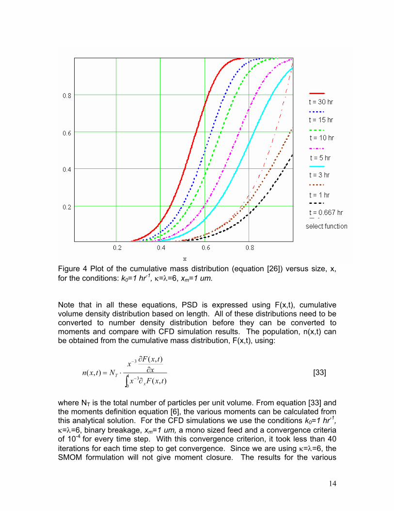
Figure 4 Plot of the cumulative mass distribution (equation [26]) versus size, x, for the conditions: k0=1 hr-1, κ=λ=6, xm=1 um. Note that in all these equations, PSD is expressed using F(x,t), cumulative volume density distribution based on length. All of these distributions need to be converted to number density distribution before they can be converted to moments and compare with CFD simulation results. The population, n(x,t) can be obtained from the cumulative mass distribution, F(x,t), using:

∫ ∂

∂∂

⋅=−

−

1

0

3

3

),(

),(

),(txFx

xtxFx

Ntxnx

T [33]

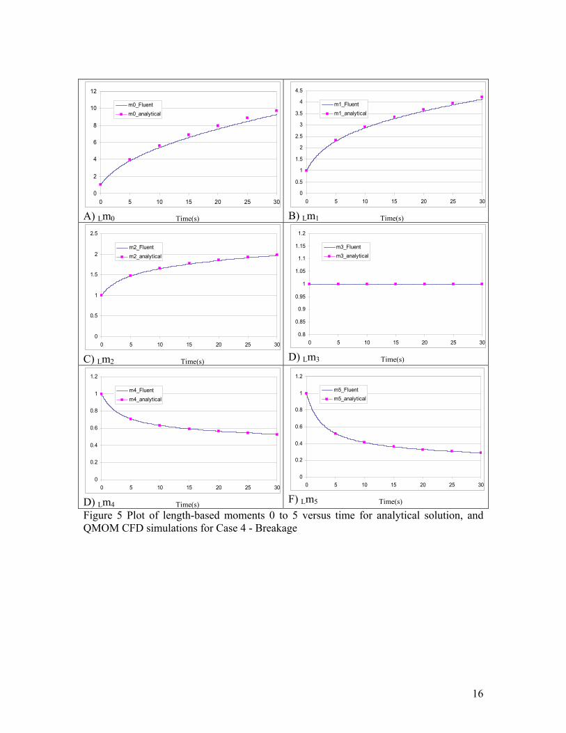
where NT is the total number of particles per unit volume. From equation [33] and the moments definition equation [6], the various moments can be calculated from this analytical solution. For the CFD simulations we use the conditions k0=1 hr-1, κ=λ=6, binary breakage, xm=1 um, a mono sized feed and a convergence criteria of 10-4 for every time step. With this convergence criterion, it took less than 40 iterations for each time step to get convergence. Since we are using κ=λ=6, the SMOM formulation will not give moment closure. The results for the various

14

moments are shown in Figure 5. Here we see exponentially increasing, 0th, 1st and 2nd moments, a constant 3rd moment corresponding to a constant mass of particles and exponentially decreasing 4th and 5th moments. These moments compare favorably with the analytical values of the moments also plotted in Figure 5. The maximum error in the moments is captured in Table 5. Here we see that the largest error is in the 0th moment, the total number of particles. The maximum error in all of the moments is 4.664% The analytical solution to the population balance for breakage can also be solved using the method of moments transformation. Starting with equations [7] and eliminating the 2nd term, the growth term, the moment transport equation is given by:

∫∞

−=0

),()()12( dvtvnvSxdtmd i

iiv η [34]

where ηi is defined by equation [8]. When S(x)=So and p(v|v’)=v/v’ the moment equation is reduced to: ivoi

iv mSdtmd

)12( −= η [35]

which can be readily solved for the various moments12: tSmtm oiiviv )12exp()0()( −= η [36] This solution gives an exponentially increasing number density (0th volume moment) and a constant total particle mass (1st volume moment and 3rd length moment) because η0=1 and η1 =1/2 due to conservation of mass as seen in Figure 5.

15

0

2

4

6

8

10

12

0 5 10 15 20 25 30

m0_Fluentm0_analytical

A) Lm0 Time(s)

0

0.5

1

1.5

2

2.5

3

3.5

4

4.5

0 5 10 15 20 25 30

m1_Fluentm1_analytical

B) Lm1 Time(s)

C) Lm2 Time(s)

0.8

0.85

0.9

0.95

1

1.05

1.1

1.15

1.2

0 5 10 15 20 25 30

m3_Fluentm3_analytical

D) Lm3 Time(s)

D) Lm4 Time(s)

0

0.2

0.4

0.6

0.8

1

1.2

0 5 10 15 20 25 30

m5_Fluentm5_analytical

F) Lm5 Time(s)

0

0.5

1

1.5

2

2.5

0 5 10 15 20 25 30

m2_Fluentm2_analytical

0

0.2

0.4

0.6

0.8

1

1.2

0 5 10 15 20 25 30

m4_Fluentm4_analytical

Figure 5 Plot of length-based moments 0 to 5 versus time for analytical solution, and QMOM CFD simulations for Case 4 - Breakage

16

Table 5 Maximum error for SMOM and QMOM CFD simulation over the time period 0 to 30s for Case 4 – Breakage. Convergence criteria is set to 10-4 for every time step

Moments Error % Lm0 4.664 Lm1 2.076 Lm2 0.825 Lm3 0 Lm4 0.515 Lm5 0.729

4. Conclusion: A two-phase model for the contents of a tank with a PBE for the solid phase has been developed and solved with either the SMOM or QMOM options within CFD code. This model has been tested using numerical cases with nucleation, growth, aggregation and breakage to validate the model. These CFD simulations are compared with analytical solutions to the batch PBE for these cases. The SMOM simulations8 can be used for cases with moment closure. The QMOM simulation can be used for all cases. The QMOM simulation accurately predicts all of these cases. To obtain less than 1% accuracy for these cases, convergence criteria less than 10-4 are necessary. The only concern about this CFD PBM code is that proper units should be used for the particle size system. For example, if we use meters for particle size, then for nano particles with size of 10-9 meters, the 6th moments will goes to order of 10-54, numerical error will be dramatic for that small number. For all the cases tested here, microns are used for particle size.

5. Nomenclature: B0 Nucleation rate F(x,t) Cumulative Mass distribution (volume density) function based

on length at time t Ka Area shape coefficient kB Boltzmann Constant Kv Volume shape coefficient Li abscissas Lmi Length based moments, i= 1, 2 …. n(x,t) Population density function N0 the initial number of particles NT Total number of particles per unit volume P(x) Cumulative daughter’s distribution function S(x) Breakage rate T Temperature t1/2 half-life

17

18

v Volume, m3

wi weights x Particle length, m

6. Literature Cited:

1 McGraw, R. (1997) Description of aerosol dynamics by the quadrature method of moments. Aerosol Science and Technology 27, 255-265 2 Randolph, A. D.; Larson, M. A. Theory of Particulate Processes, 2nd edition; New York: Academic Press, 1988 3 Hulburt, H.M. and Katz, S. Some Problems in Particle Technology – Statistical Mechanical Formulation, Chem. Eng. Sci., 1964 19, 555. 4 Prasher, C.L., Crushing and Grinding Process Handbook, New York: Wiley, 1987. 5 Randolph, A. D.; Larson, M. A. Theory of Particulate Processes, 2nd edition; New York: Academic Press, 1988 6 ibid 7 McGraw, R. (1997) Description of aerosol dynamics by the quadrature method of moments. Aerosol Science and Technology 27, 255-265. 8 Marchisio D. L., R. D. Vigil and R. Bo Fox, Implementation of the Quadrature Method of Moments in CFD codes for aggregation-breakage problems, chemical engineering science, v58, n15, August 2003. p. 3337-3351. 9 Gordon, R.G. (1968) “Error bounds in equilibrium statistical mechanics”, Journal Mathematical Physics, 9, 655-672. 10 Von Smoluchowshi, M. Z. Phys. Chem., 92, 1129-168 (1917) 11 Rajamani, R.K., Class notes “Mathematical Modeling of Extractive Metallurgical Processes,” 2003, University of Utah. 12 Ramkrishna, D., “Population Balances,” Academic Press, San Diego, CA, 2000. 13 ibid. 14 Peter King, Journal of South African Institute of Mining & Metallurgy, Nov 1972, p 127-131 15 Abramovitz and Stegun, Handbook of Mathematical Functions, Dover, New York, 1965, p.503