Variational Problems for Fefferman Hypersurface Measure and Volume-Preserving CR Invariants
37
J Geom Anal (2011) 21: 372–408 DOI 10.1007/s12220-010-9151-2 Variational Problems for Fefferman Hypersurface Measure and Volume-Preserving CR Invariants Christopher Hammond Received: 6 July 2009 / Published online: 21 July 2010 © Mathematica Josephina, Inc. 2010 Abstract We derive Euler’s equation for the isoperimetric problem and the extremal hypersurface problem associated with Fefferman hypersurface measure for strongly pseudoconvex real hypersurfaces in C 2 . We use volume-preserving CR invariants to show that the only “torsion-free” solutions of Euler’s equation for the isoperimetric problem are the volume-preserving images of spheres. 1 Introduction In [5], Fefferman introduced a measure on a smooth strongly pseudoconvex hyper- surface Z in C n , which we shall refer to as Fefferman hypersurface measure. If Z has defining function ρ , then Fefferman hypersurface measure on Z is the positive (2n − 1)-form σ Z on Z given by σ Z ∧ dρ = 2 2n/(n+1) M(ρ) 1/(n+1) ω C n , where ω C n is the Euclidean volume form and M(ρ) is the Monge–Amp ` ere operator defined by M(ρ) = (−1) n det ρ ρ z j ρ ¯ z k ρ z j , ¯ z k . Equivalently, σ Z = 2 2n/(n+1) M(ρ) 1/(n+1) |∇ ρ | s Z , Communicated by Alexander Isaev. C. Hammond ( ) Department of Mathematics, University of Michigan, Ann Arbor, MI 48109, USA e-mail: [email protected]
-
Upload
christopher-hammond -
Category
Documents
-
view
212 -
download
0
Transcript of Variational Problems for Fefferman Hypersurface Measure and Volume-Preserving CR Invariants

J Geom Anal (2011) 21: 372–408DOI 10.1007/s12220-010-9151-2
Variational Problems for Fefferman HypersurfaceMeasure and Volume-Preserving CR Invariants
Christopher Hammond
Received: 6 July 2009 / Published online: 21 July 2010© Mathematica Josephina, Inc. 2010
Abstract We derive Euler’s equation for the isoperimetric problem and the extremalhypersurface problem associated with Fefferman hypersurface measure for stronglypseudoconvex real hypersurfaces in C
2. We use volume-preserving CR invariants toshow that the only “torsion-free” solutions of Euler’s equation for the isoperimetricproblem are the volume-preserving images of spheres.
1 Introduction
In [5], Fefferman introduced a measure on a smooth strongly pseudoconvex hyper-surface Z in C
n, which we shall refer to as Fefferman hypersurface measure. If Z
has defining function ρ, then Fefferman hypersurface measure on Z is the positive(2n − 1)-form σZ on Z given by
σZ ∧ dρ = 22n/(n+1)M(ρ)1/(n+1)ωCn,
where ωCn is the Euclidean volume form and M(ρ) is the Monge–Ampere operatordefined by
M(ρ) = (−1)ndet
(ρ ρzj
ρzkρzj ,zk
).
Equivalently,
σZ = 22n/(n+1)M(ρ)1/(n+1)
|∇ρ| sZ,
Communicated by Alexander Isaev.
C. Hammond (�)Department of Mathematics, University of Michigan, Ann Arbor, MI 48109, USAe-mail: [email protected]
Variational Problems for Fefferman Measure 373
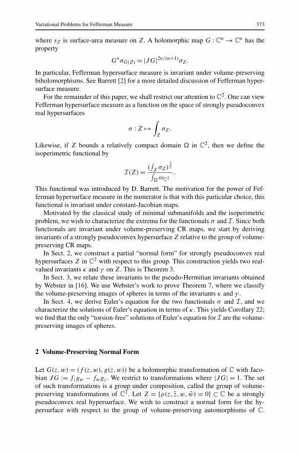
where sZ is surface-area measure on Z. A holomorphic map G : Cn → C
n has theproperty
G∗σG(Z) = |JG|2n/(n+1)σZ.
In particular, Fefferman hypersurface measure is invariant under volume-preservingbiholomorphisms. See Barrett [2] for a more detailed discussion of Fefferman hyper-surface measure.
For the remainder of this paper, we shall restrict our attention to C2. One can view
Fefferman hypersurface measure as a function on the space of strongly pseudoconvexreal hypersurfaces
σ : Z �→∫
Z
σZ.
Likewise, if Z bounds a relatively compact domain � in C2, then we define the
isoperimetric functional by
I(Z) = (∫Z
σZ)32∫
�ωC2
.
This functional was introduced by D. Barrett. The motivation for the power of Fef-ferman hypersurface measure in the numerator is that with this particular choice, thisfunctional is invariant under constant-Jacobian maps.
Motivated by the classical study of minimal submanifolds and the isoperimetricproblem, we wish to characterize the extrema for the functionals σ and I . Since bothfunctionals are invariant under volume-preserving CR maps, we start by derivinginvariants of a strongly pseudoconvex hypersurface Z relative to the group of volume-preserving CR maps.
In Sect. 2, we construct a partial “normal form” for strongly pseudoconvex realhypersurfaces Z in C
2 with respect to this group. This construction yields two real-valued invariants κ and γ on Z. This is Theorem 3.
In Sect. 3, we relate these invariants to the pseudo-Hermitian invariants obtainedby Webster in [16]. We use Webster’s work to prove Theorem 7, where we classifythe volume-preserving images of spheres in terms of the invariants κ and γ .
In Sect. 4, we derive Euler’s equation for the two functionals σ and I , and wecharacterize the solutions of Euler’s equation in terms of κ . This yields Corollary 22;we find that the only “torsion-free” solutions of Euler’s equation for I are the volume-preserving images of spheres.
2 Volume-Preserving Normal Form
Let G(z,w) = (f (z,w), g(z,w)) be a holomorphic transformation of C with Jaco-bian JG := fzgw − fwgz. We restrict to transformations where |JG| = 1. The setof such transformations is a group under composition, called the group of volume-preserving transformations of C
2. Let Z = {ρ(z, z,w, w) = 0} ⊂ C be a stronglypseudoconvex real hypersurface. We wish to construct a normal form for the hy-persurface with respect to the group of volume-preserving automorphisms of C.
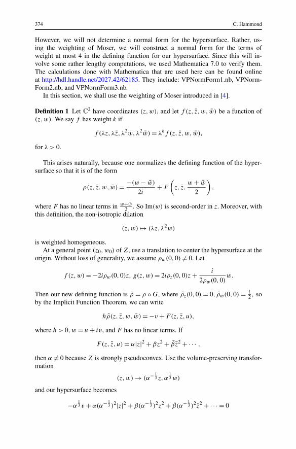
374 C. Hammond
However, we will not determine a normal form for the hypersurface. Rather, us-ing the weighting of Moser, we will construct a normal form for the terms ofweight at most 4 in the defining function for our hypersurface. Since this will in-volve some rather lengthy computations, we used Mathematica 7.0 to verify them.The calculations done with Mathematica that are used here can be found onlineat http://hdl.handle.net/2027.42/62185. They include: VPNormForm1.nb, VPNorm-Form2.nb, and VPNormForm3.nb.
In this section, we shall use the weighting of Moser introduced in [4].
Definition 1 Let C2 have coordinates (z,w), and let f (z, z,w, w) be a function of
(z,w). We say f has weight k if
f (λz,λz, λ2w,λ2w) = λkf (z, z,w, w),
for λ > 0.
This arises naturally, because one normalizes the defining function of the hyper-surface so that it is of the form
ρ(z, z,w, w) = −(w − w)
2i+ F
(z, z,
w + w
2
),
where F has no linear terms in w+w2 . So Im(w) is second-order in z. Moreover, with
this definition, the non-isotropic dilation
(z,w) �→ (λz,λ2w)
is weighted homogeneous.At a general point (z0,w0) of Z, use a translation to center the hypersurface at the
origin. Without loss of generality, we assume ρw(0,0) �= 0. Let
f (z,w) = −2iρw(0,0)z, g(z,w) = 2iρz(0,0)z + i
2ρw(0,0)w.
Then our new defining function is ρ = ρ ◦ G, where ρz(0,0) = 0, ρw(0,0) = i2 , so
by the Implicit Function Theorem, we can write
hρ(z, z,w, w) = −v + F(z, z, u),
where h > 0,w = u + iv, and F has no linear terms. If
F(z, z, u) = α|z|2 + βz2 + βz2 + · · · ,
then α �= 0 because Z is strongly pseudoconvex. Use the volume-preserving transfor-mation
(z,w) → (α− 13 z,α
13 w)
and our hypersurface becomes
−α13 v + α(α− 1
3 )2|z|2 + β(α− 13 )2z2 + β(α− 1
3 )2z2 + · · · = 0

Variational Problems for Fefferman Measure 375
or
−v + |z|2 + β
αz2 + β
αz2 + · · · = 0.
Using a rotation, we may assume β = β ≥ 0. Henceforth, we may assume that ourtransformations take the form
(z,w) → (z + bw + · · · ,w + · · · ),where b is an arbitrary constant.
Before going any further, we describe how such transformations change the equa-tion defining Z, following Moser’s approach. Suppose one begins with a hypersurfacegiven by
v∗ = F ∗(z∗, z∗, u∗) = F ∗2 + F ∗
3 + · · · ,
where F ∗i is a real-valued function of weight i as described in Definition 1, i.e.,
F ∗(λz∗, λz∗, λ2u∗) = λiF ∗(z∗, z∗, u∗), and w∗ = u∗ + iv∗. One wishes to changecoordinates via the map
(z,w) �→ (z∗,w∗) = (f (z,w), g(z,w)),
so that the new equation is
v = F(z, z, u) = F2 + F3 + · · · .
We also decompose f and g into weighted homogeneous parts, homogeneous ofweight 1 in z and of weight 2 in w. In order for the map to preserve the normalizationswe have already made, it must be the case that
f (z,w) = z + f2(z,w) + · · · and g(z,w) = w + g2(z) + g3(z,w) + · · · .
Then
Im(w∗) = F ∗(f, f , u + Re(g2(z) + g3(z,w) + · · · ))or
v + Im(g2(z)) + Im(g3(z,w)) + · · · = F ∗(f, f , u + Re(g3(z,w)) + · · · ),and finally
F = F ∗(f, f , u+Re(g2(z))+Re(g3(z,w))+· · · )−Im(g2(z))−Im(g3(z,w))−· · · .
We now use the well-known fact that any composition of shears is a volume-preserving automorphism. Consider the shear (z,w) → (z,w + az2). If our definingfunction is
ρ(z, z,w, w) = −v + |z|2 + βz2 + βz2 + · · · ,
then our new defining function is
ρ(z, z,w, w) = −v + |z|2 + βz2 + βz2 − Im(az2) + · · · .
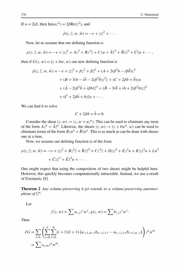
376 C. Hammond
If a = 2iβ , then Im(az2) = 2βRe(z2), and
ρ(z, z,w, w) = −v + |z|2 + · · · .
Now, let us assume that our defining function is
ρ(z, z,w, w) = −v + |z|2 + Az3 + Bz2z + Czu + Az3 + Bzz2 + Czu + · · · ,
then if G(z,w) = (z + bw,w) our new defining function is
ρ(z, z,w, w) = −v + |z|2 + βz2 + βz2 + (A + 2iβ2b − iβb)z3
+ (B + 3ib − ib − 2iβ2b)z2z + (C + 2βb + b)zu
+ (A − 2iβ2b + iβb)z3 + (B − 3ib + ib + 2iβ2b)zz2
+ (C + 2βb + b)zu + · · · .
We can find b to solve
C + 2βb + b = 0.
Consider the shear (z,w) → (z,w + azn). This can be used to eliminate any termof the form Azn + Azn. Likewise, the shears (z,w) → (z + bwn,w) can be used toeliminate terms of the form Bzun + Bzun. This is as much as can be done with shearsone at a time.
Now, we assume our defining function is of the form
ρ(z, z,w, w) = −v + |z|2 + Bz2z + Bzz2 + Cz3z + D|z|4 + Ez2u + K|z|2u + Lu2
+ Czz3 + Ez2u + · · · .
One might expect that using the composition of two shears might be helpful here.However, this quickly becomes computationally intractable. Instead, we use a resultof Forstneric [8].
Theorem 2 Any volume-preserving k-jet extends to a volume-preserving automor-phism of C
n.
Let
f (z,w) =∑
ai,j ziwj , g(z,w) =
∑bi,j z
iwj .
Then
JG =∑n,m
(n∑
i=0
m∑l=0
(i + 1)(l + 1)(ai+1,m−lbn−i,l+1 − an−i,l+1bi+1,m−l
))znwm
=∑
cn,mznwm.

Variational Problems for Fefferman Measure 377
A k-jet is volume-preserving if c0,0 = 1, cn,m = 0 for 0 < n + m ≤ k − 1. Wewould like to find a volume-preserving k-jet that will transform our defining functioninto one of the form
ρ(z, z,w, w) = −v + |z|2 + κ|z|4 + γ z3z + γ zz3 + · · · .
Since only the 4-jet of our transformation will affect these terms, we look for avolume-preserving 4-jet that accomplishes this. We do this in stages. All of the com-putations involved can be done by hand, but for convenience, they can be found inthe files on the website. Let
f (z,w) =∑
ai,j ziwj , g(z,w) =
∑bi,j z
iwj ,
where
a0,0 = b0,0 = 0, a1,0 = 1, b1,0 = 0, and b0,1 = 1.
Suppose that initially
F(z, z, u) =∑
Bj,k,lzj zkul,
then our new defining function is the graph of
F (z, z, u) =∑
Bj,k,lzj zkul.
Our new F will be F (z, z, u) = F(f (z,w), f (z,w),Re(g(z,w)))− Im(g)+v, on Z.We solve the system of equations arising from F (z, z, u) = |z|2 + F4(z, z, u) wherethe coefficients of F4 are all 0 except for possibly the coefficients of |z|4, z3z, andzz3. We also require c0,0 = 1, cn,m = 0 for 0 < n + m ≤ 3. Note that
B2,0,0 = B2,0,0 + i
2b2,0.
Since B2,0,0 = 0, we must have b2,0 = 0. Likewise,
B3,0,0 = B3,0,0 + i
2b3,0,
and since B3,0,0 = 0, we require that b3,0 = 0. With these restrictions, we have that
c0,0 = 1
c1,0 = b1,1 + 2a2,0
c0,1 = a1,1 + 2b0,2 − a0,1b1,1.
Since c1,0 = 0,
a2,0 = −1
2b1,1.

378 C. Hammond
We can choose a1,1 so that c0,1 = 0. We have
B2,1,0 = B2,1,0 + a2,0 − ia0,1 − 1
2b1,1 and B1,0,1 = B1,0,1 + a0,1 + i
2b1,1.
Since B1,0,1 = 0, B1,0,1 = 0 implies that
a0,1 = i
2b1,1.
Then B2,1,0 = 0 if and only if
b1,1 = 2
3B2,1,0.
This means that we can find the 2-jet of a volume-preserving biholomorphism suchthat our earlier normalizations are preserved and B2,1,0 = 0. Once we have B2,1,0 = 0,we impose the restrictions that b1,1 = 0, a0,1 = 0, and a2,0 = 0. Now
B4,0,0 = B4,0,0 + i
2b4,0.
Since B4,0,0 = 0, b4,0 = 0. Now we have that
c0,1 = a1,1 + 2b0,2
c2,0 = 3a3,0 + b2,1
c1,1 = 2a2,1 + 2b1,2
and
c0,2 = a1,2 + 2a1,1b0,2 + 3b0,3.
We wish to obtain the normalizations B2,0,1 = 0, B1,1,1 = 0, B0,0,2 = 0. We have
B2,0,1 = B2,0,1 + i
2b2,1
B1,1,1 = B1,1,1 + 2 Re(a1,1) − 2 Re(b0,2)
and
B0,0,2 = B0,0,2 − Im(b0,2).
Then B2,0,1 = 0 implies that
b2,1 = 2iB2,0,1.
Also c2,0 = 0 if and only if
a3,0 = −1
3b2,1
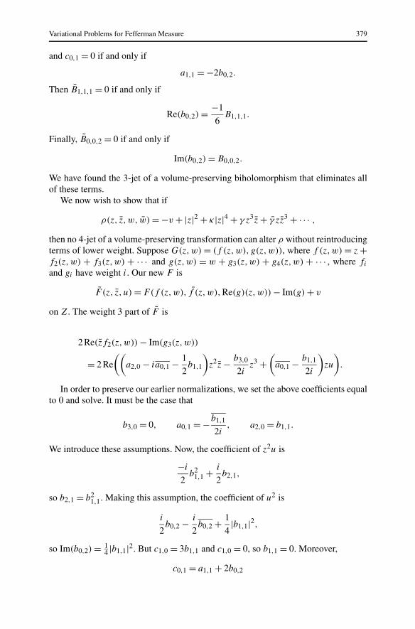
Variational Problems for Fefferman Measure 379
and c0,1 = 0 if and only if
a1,1 = −2b0,2.
Then B1,1,1 = 0 if and only if
Re(b0,2) = −1
6B1,1,1.
Finally, B0,0,2 = 0 if and only if
Im(b0,2) = B0,0,2.
We have found the 3-jet of a volume-preserving biholomorphism that eliminates allof these terms.
We now wish to show that if
ρ(z, z,w, w) = −v + |z|2 + κ|z|4 + γ z3z + γ zz3 + · · · ,
then no 4-jet of a volume-preserving transformation can alter ρ without reintroducingterms of lower weight. Suppose G(z,w) = (f (z,w), g(z,w)), where f (z,w) = z +f2(z,w) + f3(z,w) + · · · and g(z,w) = w + g3(z,w) + g4(z,w) + · · · , where fi
and gi have weight i. Our new F is
F (z, z, u) = F(f (z,w), f (z,w),Re(g)(z,w)) − Im(g) + v
on Z. The weight 3 part of F is
2 Re(zf2(z,w)) − Im(g3(z,w))
= 2 Re
((a2,0 − ia0,1 − 1
2b1,1
)z2z − b3,0
2iz3 +
(a0,1 − b1,1
2i
)zu
).
In order to preserve our earlier normalizations, we set the above coefficients equalto 0 and solve. It must be the case that
b3,0 = 0, a0,1 = −b1,1
2i, a2,0 = b1,1.
We introduce these assumptions. Now, the coefficient of z2u is
−i
2b2
1,1 + i
2b2,1,
so b2,1 = b21,1. Making this assumption, the coefficient of u2 is
i
2b0,2 − i
2b0,2 + 1
4|b1,1|2,
so Im(b0,2) = 14 |b1,1|2. But c1,0 = 3b1,1 and c1,0 = 0, so b1,1 = 0. Moreover,
c0,1 = a1,1 + 2b0,2

380 C. Hammond
so a1,1 = −2b0,2 and a1,1 is real. The new coefficient of |z|4 is
κ − 2 Im(a1,1) = κ.
Finally, 0 = c2,0 = 3a3,0 so a3,0 = 0. The new coefficient of z3z is
γ + a3,0 = γ
and we see that ρ is unchanged. Hence, we have a normal form for ρ up throughweight 4, and the coefficients κ and γ, γ represent volume-preserving invariants ofour hypersurface. Actually, we have been requiring that JG = 1, but we really needonly impose the restriction that |JG| = 1. This additional freedom allows us to use arotation in z so that γ is real and γ ≥ 0. We state this result as:
Theorem 3 Given a strongly pseudoconvex real hypersurface Z ⊂ C2 and a point
(z0,w0) ∈ Z, there exists the germ of a volume-preserving biholomorphic transfor-mation G : C
2 → C2 at (z0,w0) such that G(Z) has defining function ρ(z,w) =
−v + |z|2 + κ|z|4 + γ z3z + γ zz3 + · · · , where all other terms have weight greaterthan 4 and γ is real. Moreover, if there exists any other such germ of a biholomor-phic volume-preserving transformation G : C
2 → C2 such that G(Z) has a defining
function ρ(z,w) = −v +|z|2 + κ|z|4 + γ z3z+ γ zz3 +· · · where all other terms haveweight greater than 4 and γ is real, then κ = κ and γ = γ .
3 Classification of Volume-Preserving Images of Spheres
In this section, we will use a theorem of S. Webster [16] to determine when it ispossible to find a volume-preserving CR isomorphism between a general stronglypseudoconvex real hypersurface Z in C
2 and the sphere of radius R. Webster’s workis inspired by S. S. Chern, who uses techniques invented by E. Cartan. Before pro-ceeding, we want to indicate how Cartan’s approach works in general. This was suc-cinctly and lucidly explained by Burns and Shnider [3]. The following explanation istaken from there almost verbatim, changing only notation. Associate with any man-ifold Z with the given structure a second manifold P , fibered over Z, such that anystructure-preserving map f lifts to an f for which the following diagram commutes:
P1f−−−−→ P2
π1
⏐⏐� π2
⏐⏐�Z1
f−−−−→ Z2
Then define on P a parallelism, i.e., a trivialization of the tangent bundle (equiv-alently, define a coframe �), such that the maps g : P1 → P2 of the form f areprecisely those for which dg carries the parallelism of P1 onto that of P2 (equiv-alently, such that g∗�2 = �1). Having reduced the problem to maps preserving agiven parallelism (equivalently, coframe), one can use a theorem of Cartan to solvethe problem.
Variational Problems for Fefferman Measure 381
In order to state the theorem, one needs some auxiliary definitions. Our expositionfollows Olver in [14]. Let M be an n-dimensional manifold. We define K
(s)(n), thes-th order classifying space, to be Euclidean space of dimension qs(n) = 1
2n2(n −1)
(n+sn
), where the coordinates are indexed by zσ , where σ = (i, j, k, l1, . . . , ls) is a
multi-index of order s. Given a coframe � = (θ1, . . . , θn) and a function f on M ,
we have that df = ∑aj θ
j . We define ∂f
∂θj = aj . Let Tσ = ∂sT ij,k
∂θ ls ···∂θl1, where � =
(θ1, . . . , θn) is a coframe and dθi = ∑T i
j,kθj ∧ θk . Define the s-th order structure
map T(s) : M → K(s) by zσ = Tσ (x). The s-th classifying space C(s)(θ,M) is the
image of T(s). We say that a coframe � is fully regular if for all s, the s-th orderstructure map is regular, i.e., has constant rank rs . Note that rs is the number offunctionally independent structure invariants up to order s. Finally, we define theorder of the coframe � to be the smallest s for which rs = rs+1. Cartan proved:
Theorem 4 Let � and � be smooth, fully regular coframes on M and M , respec-tively. Then there exists a local diffeomorphism � : M → M with �∗� = � if andonly if they have the same order s − 1 = s − 1 and C(s)(�,U) ∩ C(s)(�, U ) is anon-empty submanifold of K(s)(m) with the same dimension as C(s)(�,U), whereU ⊂ M and U ⊂ M are open neighborhoods.
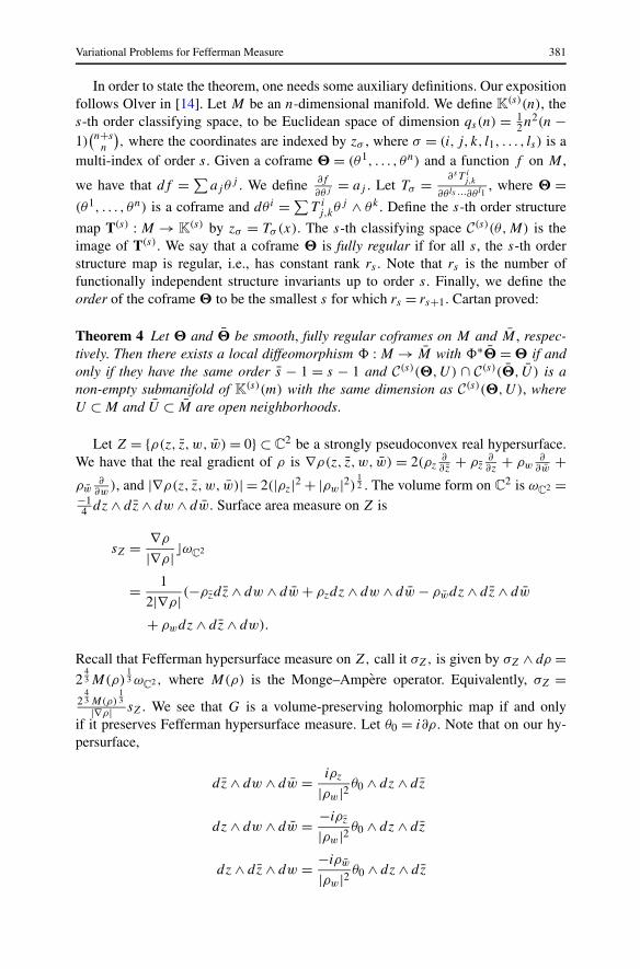
Let Z = {ρ(z, z,w, w) = 0} ⊂ C2 be a strongly pseudoconvex real hypersurface.
We have that the real gradient of ρ is ∇ρ(z, z,w, w) = 2(ρz∂∂z
+ ρz∂∂z
+ ρw∂
∂w+
ρw∂
∂w), and |∇ρ(z, z,w, w)| = 2(|ρz|2 + |ρw|2) 1
2 . The volume form on C2 is ωC2 =
−14 dz ∧ dz ∧ dw ∧ dw. Surface area measure on Z is
sZ = ∇ρ
|∇ρ| �ωC2
= 1
2|∇ρ| (−ρzdz ∧ dw ∧ dw + ρzdz ∧ dw ∧ dw − ρwdz ∧ dz ∧ dw
+ ρwdz ∧ dz ∧ dw).
Recall that Fefferman hypersurface measure on Z, call it σZ, is given by σZ ∧ dρ =2
43 M(ρ)
13 ωC2, where M(ρ) is the Monge–Ampere operator. Equivalently, σZ =
243 M(ρ)
13
|∇ρ| sZ. We see that G is a volume-preserving holomorphic map if and onlyif it preserves Fefferman hypersurface measure. Let θ0 = i∂ρ. Note that on our hy-persurface,
dz ∧ dw ∧ dw = iρz
|ρw|2 θ0 ∧ dz ∧ dz
dz ∧ dw ∧ dw = −iρz
|ρw|2 θ0 ∧ dz ∧ dz
dz ∧ dz ∧ dw = −iρw
|ρw|2 θ0 ∧ dz ∧ dz
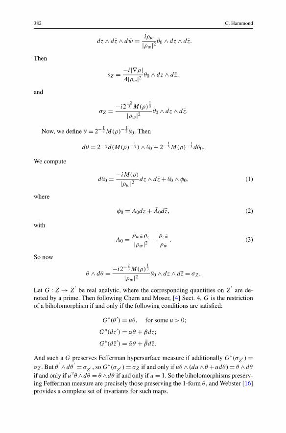
382 C. Hammond
dz ∧ dz ∧ dw = iρw
|ρw|2 θ0 ∧ dz ∧ dz.
Then
sZ = −i|∇ρ|4|ρw|2 θ0 ∧ dz ∧ dz,
and
σZ = −i2−23 M(ρ)
13
|ρw|2 θ0 ∧ dz ∧ dz.
Now, we define θ = 2− 13 M(ρ)− 1
3 θ0. Then
dθ = 2− 13 d(M(ρ)−
13 ) ∧ θ0 + 2− 1
3 M(ρ)−13 dθ0.
We compute
dθ0 = −iM(ρ)
|ρw|2 dz ∧ dz + θ0 ∧ φ0, (1)
where
φ0 = A0dz + A0dz, (2)
with
A0 = ρwwρz
|ρw|2 − ρzw
ρw
. (3)
So now
θ ∧ dθ = −i2− 23 M(ρ)
13
|ρw|2 θ0 ∧ dz ∧ dz = σZ.
Let G : Z → Z′
be real analytic, where the corresponding quantities on Z′
are de-noted by a prime. Then following Chern and Moser, [4] Sect. 4, G is the restrictionof a biholomorphism if and only if the following conditions are satisfied:
G∗(θ ′) = uθ, for some u > 0;G∗(dz′) = αθ + βdz;G∗(dz′) = αθ + βdz.
And such a G preserves Fefferman hypersurface measure if additionally G∗(σZ
′ ) =σZ . But θ
′ ∧dθ′ = σ
Z′ , so G∗(σ
Z′ ) = σZ if and only if uθ ∧ (du∧θ +udθ) = θ ∧dθ
if and only if u2θ ∧dθ = θ ∧dθ if and only if u = 1. So the biholomorphisms preserv-ing Fefferman measure are precisely those preserving the 1-form θ , and Webster [16]provides a complete set of invariants for such maps.

Variational Problems for Fefferman Measure 383
On our hypersurface Z,
θ0 = θ0, dw = −i
ρw
θ0 − ρz
ρw
dz, dw = i
ρw
θ0 − ρz
ρw
dz.
For a function f on a neighborhood of Z, the restriction of df to Z satisfies
df = fzdz + fzdz + fwdw + fwdw
= fzdz + fzdz +(−ifw
ρw
θ0 − ρz
ρw
fwdz
)+
(ifw
ρw
θ0 − ρz
ρw
fwdz
)
=(−i
ρw
fw + i
ρw
fw
)θ0 +
(fz − ρz
ρw
fw
)dz +
(fz − ρz
ρw
fw
)dz.
So if X, X1, X1 is the dual frame to θ0, dz, dz, then X = iρw
∂∂w
− iρw
∂∂w
, X1 = ∂∂z
−ρz
ρw
∂∂w
, and X1 = ∂∂z
− ρz
ρw
∂∂w
.
Then
dθ0 = idρz ∧ dz + idρw ∧ dw
= i(X(ρz)θ0 + X1(ρz)dz + X1(ρz)dz
)∧ dz
i(X(ρw)θ0 + X1(ρw)dz + X1(ρw)dz
)∧
(−i
ρw
θ0 − ρz
ρw
dz
)
= −iM(ρ)
|ρw|2 dz ∧ dz + θ0 ∧ φ0,
where φ0 and A0 are as in (1)–(3). Note that we have repeated some earlier workbecause we wish to relate these quantities to X, X1, and X1.
We have
dθ = 2− 13 d(M− 1
3 ) ∧ θ0 + 2− 13 M− 1
3 dθ0
= −2− 13
3M− 4
3 dM ∧ θ0 + 2− 13 M− 1
3 dθ0
= θ ∧(
1
3MdM
)+ 2− 1
3 M− 13 dθ0
= 1
3Mθ ∧
(X(M)θ0 + X1(M)dz + X1(M)dz
)
+ 2− 13 M− 1
3
(−iM
|ρw|2)
dz ∧ dz + 2− 13 M− 1
3 θ0 ∧ φ0
= −i2− 13 M
23
|ρw|2 dz ∧ dz + θ ∧(
1
3MX1(M)dz + 1
3MX1(M)dz + φ0
).
So we let
A = ρw,wρz − ρz,wρw
|ρw|2 + 1
3M
(∂M
∂z− ρz
ρw
∂M
∂w
)(4)

384 C. Hammond
and
φ = Adz + Adz. (5)
We also let
g1,1 = −2−13 M
23
|ρw|2 . (6)
Then
dθ = ig1,1dz ∧ dz + θ ∧ φ. (7)
We are going to follow Webster in [16]. We are seeking 1-forms that satisfy certainrelations. This corresponds to finding an “adapted” coframe on a bundle P over Z
that depends only on the pseudo-Hermitian structure of Z. We are going throughWebster’s construction because we will need explicit formulas for the differentialinvariants that he obtains.
Now we substitute
θ1 = dz + iη1θ
θ 1 = dz − iη1θ.(8)
Note that θ1 depends on our choice of η1. Then
ig1,1θ1 ∧ θ 1 = ig1,1
(dz + iη1θ
)∧
(dz − iη1θ
)
= ig1,1dz ∧ dz + θ ∧(−g1,1η
1dz − g1,1η1dz
)
= ig1,1dz ∧ dz + θ ∧ φ.
Together with (7), this implies that if we take η1 = −1g1,1
A, we will have
dθ = ig1,1θ1 ∧ θ 1. (9)
At this stage, we must introduce the bundle P which was alluded to earlier. Let(θ, θ1, θ 1) be any coframe where θ1 is a (1,0)-form, i.e., θ1 = dz + iη1θ and θ
is the 1-form defining the pseudo-Hermitian structure on Z. We call this coframeadmissible if it satisfies condition (9). We define P to be the bundle of admissiblecoframes on Z. If (θ, θ1, θ 1) is an admissible coframe, then any other admissiblecoframe is of the form
(θ, θ1, θ 1) = (θ, u11θ
1, u11θ 1),
where u11 : Z → C
∗. Hence the fiber of P over z ∈ Z is
(θ, u11θ
1, u11θ 1),

Variational Problems for Fefferman Measure 385
where u11 ∈ C
∗. Taking u11 as a fiber coordinate, this defines a local trivialization of P ,
φ : P → Z × C∗,
which is given by
φ(z, (θ, u11θ
1, u11θ 1)) = (z, u1
1).
If (θ, θ1, θ 1) is another admissible coframe with corresponding trivialization φ : P →Z × C
∗, then recall that
(θ, θ1, θ 1) = (θ, v11 θ1, v1
1θ 1),
for some v11 : Z → C
∗. We then have the corresponding transition map T : Z ×C∗ →
Z × C∗, given by
T = φ ◦ φ−1.
Note that
T (z,u11) = (z, v1
1(z)u11) = (z, u1
1).
We define 1-forms �,�1, and �1 on the local trivialization of P by
� = θ
�1 = u11θ
1
�1 = u11θ 1.
We have the corresponding 1-forms �,�1, �1 on the trivialization φ. Note thatT ∗� = � and
T ∗�1 = T ∗(u11θ
1) =((v1
1(z))−1u11
)(v1
1(z)θ1)
= u11θ
1 = �1.
Hence �,�1,�1 correspond to 1-forms on P . We shall sometimes abuse languageand refer to these 1-forms as 1-forms on P . We have that
d� = iG1,1�1 ∧ �1, (10)
where G1,1 is a function on P . If (θ, θ1, θ 1) satisfy (9), then in the correspondingtrivialization,
G1,1 = g1,1
|u11|2
. (11)
Webster shows that there exist uniquely determined, intrinsically defined 1-formsω1
1,ω11, τ 1, and τ 1 on P satisfying:
d�1 = �1 ∧ ω11 + � ∧ τ 1 (12)
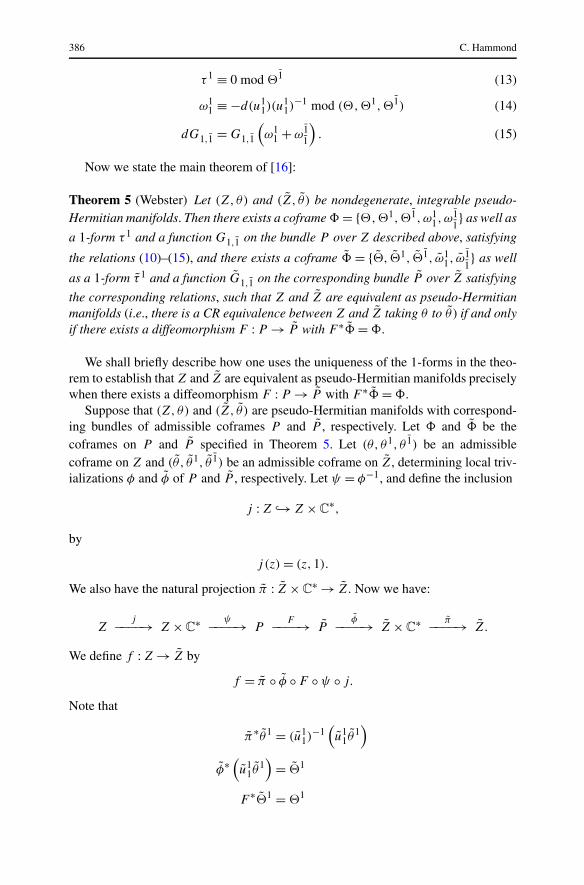
386 C. Hammond
τ 1 ≡ 0 mod �1 (13)
ω11 ≡ −d(u1
1)(u11)
−1 mod (�,�1,�1) (14)
dG1,1 = G1,1
(ω1
1 + ω11
). (15)
Now we state the main theorem of [16]:
Theorem 5 (Webster) Let (Z, θ) and (Z, θ ) be nondegenerate, integrable pseudo-Hermitian manifolds. Then there exists a coframe � = {�,�1,�1,ω1
1,ω11} as well as
a 1-form τ 1 and a function G1,1 on the bundle P over Z described above, satisfying
the relations (10)–(15), and there exists a coframe � = {�, �1, �1, ω11, ω
11} as well
as a 1-form τ 1 and a function G1,1 on the corresponding bundle P over Z satisfying
the corresponding relations, such that Z and Z are equivalent as pseudo-Hermitianmanifolds (i.e., there is a CR equivalence between Z and Z taking θ to θ ) if and onlyif there exists a diffeomorphism F : P → P with F ∗� = �.
We shall briefly describe how one uses the uniqueness of the 1-forms in the theo-rem to establish that Z and Z are equivalent as pseudo-Hermitian manifolds preciselywhen there exists a diffeomorphism F : P → P with F ∗� = �.
Suppose that (Z, θ) and (Z, θ ) are pseudo-Hermitian manifolds with correspond-ing bundles of admissible coframes P and P , respectively. Let � and � be thecoframes on P and P specified in Theorem 5. Let (θ, θ1, θ 1) be an admissiblecoframe on Z and (θ , θ1, θ 1) be an admissible coframe on Z, determining local triv-ializations φ and φ of P and P , respectively. Let ψ = φ−1, and define the inclusion
j : Z ↪→ Z × C∗,
by
j (z) = (z,1).
We also have the natural projection π : Z × C∗ → Z. Now we have:
Zj−−−−→ Z × C
∗ ψ−−−−→ PF−−−−→ P
φ−−−−→ Z × C∗ π−−−−→ Z.
We define f : Z → Z by
f = π ◦ φ ◦ F ◦ ψ ◦ j.
Note that
π∗θ1 = (u11)
−1(u1
1θ1)
φ∗ (u1
1θ1)
= �1
F ∗�1 = �1
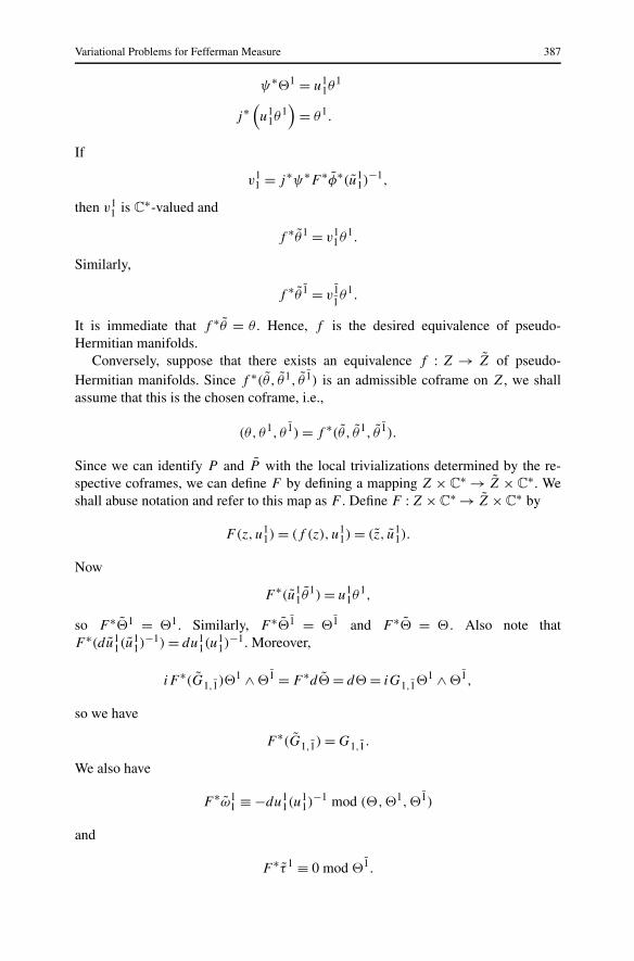
Variational Problems for Fefferman Measure 387
ψ∗�1 = u11θ
1
j∗ (u1
1θ1)
= θ1.
If
v11 = j∗ψ∗F ∗φ∗(u1
1)−1,
then v11 is C
∗-valued and
f ∗θ1 = v11θ1.
Similarly,
f ∗θ 1 = v11θ1.
It is immediate that f ∗θ = θ. Hence, f is the desired equivalence of pseudo-Hermitian manifolds.
Conversely, suppose that there exists an equivalence f : Z → Z of pseudo-Hermitian manifolds. Since f ∗(θ , θ1, θ 1) is an admissible coframe on Z, we shallassume that this is the chosen coframe, i.e.,
(θ, θ1, θ 1) = f ∗(θ , θ1, θ 1).
Since we can identify P and P with the local trivializations determined by the re-spective coframes, we can define F by defining a mapping Z × C
∗ → Z × C∗. We
shall abuse notation and refer to this map as F . Define F : Z × C∗ → Z × C
∗ by
F(z,u11) = (f (z), u1
1) = (z, u11).
Now
F ∗(u11θ
1) = u11θ
1,
so F ∗�1 = �1. Similarly, F ∗�1 = �1 and F ∗� = �. Also note thatF ∗(du1
1(u11)
−1) = du11(u
11)
−1. Moreover,
iF ∗(G1,1)�1 ∧ �1 = F ∗d� = d� = iG1,1�
1 ∧ �1,
so we have
F ∗(G1,1) = G1,1.
We also have
F ∗ω11 ≡ −du1
1(u11)
−1 mod (�,�1,�1)
and
F ∗τ 1 ≡ 0 mod �1.
388 C. Hammond
Moreover,
d�1 = F ∗d�1 = F ∗ (�1 ∧ ω1
1 + � ∧ τ 1)
= �1 ∧ F ∗ω11 + � ∧ F ∗τ 1
and
dG1,1 = F ∗dG1,1 = G1,1
(F ∗ω1
1 + F ∗ω11
).
Therefore, by the uniqueness of ω11 and τ 1, we must have that
F ∗ω11 = ω1
1 and F ∗τ 1 = τ 1.
Hence, we have found a diffeomorphism F : P → P such that F ∗� = �.Webster then defines
�11 = dω1
1. (16)
He also defines
�1 = dτ 1 − τ 1 ∧ ω11. (17)
He shows that (see [16] p. 31)
�11 = R1
1,1,1�1 ∧ �1 + W 1
1,1�1 ∧ � − W 1
1,1�1 ∧ �, (18)
and
�1 = W 11,1
�1 ∧ �1 − A11τ 1 ∧ � + B1
1�1 ∧ �. (19)
Webster notes ([16] p. 33) that if we compute �11 in the local trivialization of P
determined by the admissible coframe (θ, θ1, θ 1), and if we compute �11 in the local
trivialization determined by another admissible coframe (θ, θ1, θ 1), then (at least inC
2)
�11 = �1
1. (20)
At this stage, we note that in order to explicitly compute the associated invariants,it will be convenient to work with 1-forms on the hypersurface Z. Again, we workon the local trivialization of P determined by an admissible coframe (θ, θ1, θ 1), i.e.,P ∼= Z × C
∗. We recall that we have an inclusion j : Z ↪→ Z × C∗ given by
j (z) = (z,1).
Then we can pull back our coframe on P to obtain 1-forms on Z. We already havethat j∗� = θ and j∗�1 = θ1. We define
μ11 = j∗ω1
1 and γ 1 = j∗τ 1.
Variational Problems for Fefferman Measure 389
Then we obtain analogues of relations (10)–(15) for these 1-forms.
dθ = ig1,1θ1 ∧ θ 1 (21)
dθ1 = θ1 ∧ μ11 + θ ∧ γ 1 (22)
γ 1 ≡ 0 mod θ1 (23)
μ11 ≡ 0 mod (θ, θ1, θ 1) (24)
dg1,1 = g1,1
(μ1
1 + μ11
). (25)
Of course, (24) is a trivial consequence of the fact that (θ, θ1, θ 1) is a coframe onZ, and so is no real constraint. Now, we can use the relations (21)–(25) to obtain“invariants” that depend on the fiber coordinates, and then find the invariants on P interms of these. For instance, we have already seen in (11) that
G1,1 = g1,1
|u11|2
.
In fact, we shall only need explicit formulas for two of the invariants.Let
dμ11 ≡ r1
1,1,1θ1 ∧ θ 1 mod θ
γ 1 = a11θ 1.
Now, from
dω11 ≡ R1
1,1,1�1 ∧ �1 mod �
τ 1 = A11�1,
we deduce
R11,1,1
=r1
1,1,1
|u11|2
(26)
A11
= u11
u11
a11. (27)
It follows from (11) and (26) that
R1,11,1
def=R1
1,1,1
G1,1
is constant on fibers and
R1,11,1 =
r11,1,1
g1,1.
390 C. Hammond
Likewise, from (27), |A11| is constant on fibers and
|A11| = |a1
1|.
Therefore, in order to compute these invariants on P , it suffices to choose an admis-sible coframe on Z and find 1-forms μ1
1 and γ 1 satisfying the relations (21)–(25)and compute the corresponding quantities for these 1-forms. While computing theseinvariants, we shall refer to these 1-forms as ω1
1 and τ 1, and unless we explicitly statethat we are working on the bundle P , everything is occurring on the hypersurface Z.So what we shall be calling ω1
1, τ1 and A1
1are really the quantities that we have been
referring to as μ11, γ
1 and a11, respectively. This is what Webster does in [16], and we
shall use several of his computations from that paper.Now, we work toward finding such 1-forms on Z. Let θ, θ1, θ 1 have dual frame
X,X1,X1. Using the relation that for any function f on Z, we must have
X(f )θ0 + X1(f )dz + X1(f )dz = X(f )θ + X1(f )θ1 + X1(f )θ 1,
we obtain X1 = X1,X1 = X1, and
X = −iη1 ∂
∂z+ iη1 ∂
∂z+
(−i2
13 M
13
ρw
+ iρz
ρw
η1
)∂
∂w+
(i2
13 M
13
ρw
+ −iρz
ρw
η1
)∂
∂w.
Now we want to find A11
such that if we define τ 1 = A11θ 1, there exists ω1
1 suchthat
dθ1 = θ1 ∧ ω11 + θ ∧ τ 1.
Using (8) and (9), we have
dθ1 = idη1 ∧ θ + iη1dθ
= i(X(η1)θ + X1(η
1)θ1 + X1(η1)θ 1
)∧ θ + iη1
(ig1,1θ
1 ∧ θ 1)
= θ1 ∧(−g1,1η
1θ 1 + iX1(η1)θ
)+ θ ∧ (−iX1(η
1)θ 1).
So A11= −iX1(η
1), and ω11 = −g1,1η
1θ 1 + iX1(η1)θ . Now we wish to adjust ω1
1 by
a multiple of θ1 to obtain a unique ω11 with dg1,1 = g1,1(ω
11 + ω1
1). We have that
dg1,1 − g1,1ω11 − g1,1ω
11
= (X(g1,1) − ig1,1X1(η1) + ig1,1X1(η
1))θ + (X1(g1,1) + g21,1
η1)θ1
+ (X1(g1,1) + g21,1
η1)θ 1
= (X1(g1,1) + g21,1
η1)θ1 + (X1(g1,1) + g21,1
η1)θ 1,
Variational Problems for Fefferman Measure 391
since the coefficient of θ must vanish (see Webster [16] p. 28). Then, again followingWebster, we can define ω1
1 by
ω1,1 = ω11g1,1 = B1,1,1θ
1 + C1,1,1θ1 + E1,1θ,
where B1,1,1 = X1(g1,1) + g21,1
η1, C1,1,1 = −g21,1
η1, and E1,1 = ig1,1X1(η1). Note
that we are using g1,1 to raise and lower indices, i.e., by definition, ω1,1 = ω11g1,1.
Likewise, replacing all indices with a bar denotes the conjugate of a quantity, so
ω11= ω1
1. To simplify notation, we shall write ω11 = Bθ1 +Cθ 1 +Eθ . To summarize,
we have:
dθ1 = θ1 ∧ ω11 + θ ∧ τ 1 (28)
τ 1 = A11θ 1 (29)
dg1,1 = g1,1(ω11 + ω1
1). (30)
Now we define �11 = dω1
1 = R11,1,1
θ1 ∧θ 1 +W 11,1θ
1 ∧θ −W 11,1
θ 1 ∧θ . We compute
dω11 = dB ∧ θ1 + Bdθ1 + dC ∧ θ 1 + Cdθ 1 + dE ∧ θ + Edθ
= (X(B)θ + X1(B)θ1 + X1(B)θ 1) ∧ θ1 + B(θ1 ∧ ω11 + θ ∧ τ 1)
+ (X(C)θ + X1(C)θ1 + X1(C)θ 1) ∧ θ 1 + C(θ 1 ∧ ω11+ θ ∧ τ 1) + dE ∧ θ
+ E(ig1,1θ1 ∧ θ 1)
= (X1(C) − X1(B) + ig1,1E + BC − |C|2)θ1 ∧ θ 1 + · · · .
Hence R11,1,1
= X1(C)−X1(B)+ ig1,1E+BC−|C|2. And finally, we define R1,11,1 =
1g1,1
R11,1,1
.
We shall compute these invariants for the sphere of radius R. Let ρ(z, z,w, w) =|z|2 + |w|2 − R2. Then M(ρ) = |z|2 + |w|2. A = z
|w|2 , g1,1 = −2−13
|w|2 (|z|2 + |w|2) 23 ,
and η1 = 213 z(|z|2 + |w|2)−2
3 . We compute A11 = −iX1(η
1) = −i(∂η1
∂z− ρz
ρw
∂η1
∂w) = 0
and hence τ 1 = 0. We also have ω11 = Bθ1 + Cθ 1 + Eθ , where B = 1
g1,1X1(g1,1) +
g1,1η1 = 0,C = −g1,1η
1, and E = iX1(η1). We compute E = i2
13 (|z|2 + |w|2)−2
3
and C = z
|w|2 , so ω11 = i2
13 (|z|2 + |w|2)−2
3 θ + z
|w|2 θ 1. Before proceeding, note that
since (|z|2 + |w|2) = ρ(z, z,w, w) + R2,X1((|z|2 + |w|2)) = X1((|z|2 + |w|2)) = 0.Now,
dω11 = 2
13 i(|z|2 + |w|2)−2
3 dθ +(
X
(z
|w|2)
θ + X1
(z
|w|2)
θ1 + X1
(z
|w|2)
θ 1)
∧ θ 1 + z
|w|2 dθ 1
392 C. Hammond
= 213 i(|z|2 + |w|2)−2
3 (ig1,1)θ1 ∧ θ 1 + X
(z
|w|2)
θ ∧ θ 1 + X1
(z
|w|2)
θ1 ∧ θ 1
+ z
|w|2 θ 1 ∧ ω11.
The last equality is because τ 1 = 0. We now substitute ω11= −i2
13 (|z|2 +|w|2)−2
3 θ +z
|w|2 θ1 and compute. We find that the above expression reduces to dω11 = 2
|w|2 θ1 ∧θ 1.We then have
Proposition 6 For the sphere of radius R in C2,
R1,11,1 = 1
g1,1R1
1,1,1
= −243 (|z|2 + |w|2)−2
3 = −243 R
−43 ,
and τ 1 = 0.
Since it will prove to be quite useful, we will now find a simplified expres-sion for R
1,11,1 assuming that we have chosen a defining function ρ such that
M(ρ) = 1 + O(ρ3) (according to Fefferman [5], this is always possible). Then
A = 1|ρw |2 (ρw,wρz − ρz,wρw) + O(ρ2) and g1,1 = −2
−13
|ρw |2 + O(ρ3). So η1 = −1g1,1
A =2
13 (ρw,wρz −ρz,wρw)+ O(ρ2). Moreover, B = 1
g1,1X1(g1,1)+g1,1η
1,C = −g1,1η1,
and E = iX1(η1). Then we have R1
1,1,1= X1(C)−X1(B)+ ig1,1E +BC −|C|2 and
so
R1,11,1 = 1
g1,1X1(C) − 1
g1,1X1(B) + iE + 1
g1,1BC − 1
g1,1|C|2
= 1
g1,1X1(−g1,1η
1) − 1
g1,1X1
(1
g1,1X1(g1,1)
)− 1
g1,1X1(g1,1η
1)
− X1(η1) + 1
g1,1
(1
g1,1X1(g1,1) + g1,1η
1)
(−g1,1η1) − g1,1|η1|2.
This simplifies to
R1,11,1 = − 1
g1,1X1(g1,1η
1) − 1
g1,1X1(g1,1η
1)
− 1
g1,1X1
(1
g1,1X1(g1,1)
)− X1(η
1) − η1
g1,1X1(g1,1) − 2g1,1|η1|2.
Now, substituting our formula for g1,1, we find that
1
g1,1X1(g1,1) = −g1,1η
1 + 1
ρ2w
(ρw,wρz − ρz,wρw) + O(ρ2).
Variational Problems for Fefferman Measure 393
Substituting this back into our expression for R1,11,1 , we obtain
R1,11,1 = −2X1(η
1) − 2η1
g1,1X1(g1,1) − 1
g1,1X1
(1
ρ2w
(ρw,wρz − ρz,wρw)
)− 2g1,1|η1|2
+ O(ρ).
Again using our formula for 1g1,1
X1(g1,1), we find that
R1,11,1 = −2X1(η
1) − 2η1
ρ2w
(ρw,wρz − ρz,wρw) − 1
g1,1X1
(1
ρ2w
(ρw,wρz − ρz,wρw)
)
+ O(ρ).
More direct computation shows us that X1(1
ρ2w(ρw,wρz − ρz,wρw)) =
−2( 1ρ2
w(ρw,wρz − ρz,wρw))g1,1η
1 + 1ρ2
wX1(ρw,wρz − ρz,wρw) + O(ρ2). Then we
have R1,11,1 = −2X1(η
1) + 213 |ρw |2ρ2
wX1(ρw,wρz − ρz,wρw) + O(ρ). At this stage, com-
puting both quantities, as well as ∂M(ρ)∂w
, we find that
R1,11,1 = 2
13 (2(ρz,wρz,w − ρz,zρw,w) + 1
ρw
(Mw + (ρz,wρz,w − ρz,zρw,w)ρw)) + O(ρ)
= 213 3(ρz,wρz,w − ρz,zρw,w) + O(ρ),
where the last equality is because Mw = 0 + O(ρ2). Therefore, on our hypersurface,
R1,11,1 = 2
13 3(ρz,wρz,w − ρz,zρw,w). (31)
If G(z,w) = (f (z,w), g(z,w)) is a volume-preserving local biholomorphism, thenif we set ρ = ρ ◦ G, direct computation yields that
M(ρ) = 1 + O(ρ3) (32)
and
(ρz,wρz,w − ρz,zρw,w) = (ρz,wρz,w − ρz,zρw,w). (33)
So we see again that R1,11,1 is an absolute invariant with respect to volume-preserving
local biholomorphisms.Now we wish to find the relationship between R
1,11,1 and our invariants κ and γ .
For this purpose, we adopt a ghastly notation. We shall write
R(zj1 zk1ul1 , . . . , zjq zkq ulq )
to denote a sum of the form
Kj1,k1,l1zj1 zk1ul1 + · · · + Kjq,kq ,lq z
jq zkq ulq
394 C. Hammond
for some arbitrary constants Kjm,km,lm with m = 1, . . . , q together with terms of ordergreater than or equal to 5. Suppose that our defining function is in normal form, so
ρ(z, z,w, w)
= −w − w
2i+ |z|2 + κ|z|4 + γ z3z + γ zz3
+ R(u3, zu2, zu2, u4, zu3, zu3, z2u2, z2u2, |z|2u2, z3u, z3u, z2zu, zz2u).
Then
M(ρ) = 1
4(1 + 4κ|z|2 + 3γ z2 + 3γ z2)
+ R(u2, zu, zu, |z|2u, zu2, zu2, z2u, z2u, z3, z3, z2z, zz2, |z|2u2, z2zu,
zz2u, z3z, zz3, |z|4).Also note that Mz = κz + 3
2γ z + R(u, zu, zu,u2, z2, z2, |z|2) andMw = R(u, z, z, |z|2, zu, zu, |z|2, z2, z2). We then have that
A = 4
3
(κz + 3
2γ z
)
+ R(u, zu, zu,u2, |z|2u, zu2, zu2, z2u, z2u, z3, z3, z2z, zz2, |z|2u2, z2zu, zz2u,
z3z, zz3, |z|4).We also find that
g1,1 = −213
(1 + 8
3κ|z|2 + 2γ z2 + 2γ z2
)
+ R(u2, zu, zu, |z|2u, zu2, zu2, z2u, z2u, z3, z3, z2z, zz2, |z|2u2, z2zu, zz2u,
z3z, zz3, |z|4)and
η1 = 2−13
4
3
(κz + 3
2γ z
)
+ R(u, zu, zu, , u2, |z|2u, zu2, zu2, z2u, z2u, z3, z3, z2z, zz2, |z|2u2, z2zu,
zz2u, z3z, zz3, |z|4).Then
R1,11,1 = −1
g1,1X1(g1,1η
1) − 1
g1,1X1(g1,1η
1) − 1
g1,1X1
(1
g1,1X1(g1,1)
)− X1(η
1)
− η1
g1,1X1(g1,1) − 2g1,1|η1|2.

Variational Problems for Fefferman Measure 395
We need to compute
X1(η1) = 2
−13
4
3κ + R(u, z, |z|2, z2, z2, u2, zu, zu, . . . ),
X1(η1) = 2
−13
4
3κ + R(u, z, |z|2, z2, z2, u2, zu, zu, . . . ),
and
1
g1,1X1(g1,1) = 8
3κz + 4γ z
+ R(u, zu, zu,u2, |z|2u, zu2, zu2, z2u, z2u, z3, z3, z2z, zz2, |z|2u2,
z2zu, zz2u, z3z, zz3, |z|4),
so 1g1,1
X1(1
g1,1X1(g1,1)) = −2
−13 8
3κ + R(z, u, . . . ). So we find that, at the origin,
R1,11,1 = −2
53
3κ. (34)
Our expression for η1 also allows us to compute A11. Recall that A1
1= −iX1(η
1).Using the above expression, we see that at the origin,
A11= −i2
23 γ. (35)
Therefore A11= 0 at a point precisely when γ = 0.
We are now in a position to prove the following:
Theorem 7 Let Z = {ρ(z, z,w, w = 0} ⊂ C2 be a strongly pseudoconvex, real-
analytic real hypersurface. Then there exists a locally volume-preserving CR equiva-
lence between Z and the sphere of radius R if and only if R1,11,1 ≡ 2
43 R
−43 , and A1
1≡ 0.
Proof By Theorem 5, this reduces to showing an equivalence of the coframes definedon the corresponding coframe bundles P and P ′ for Z and the sphere, respectively.Cartan provides us with the means of solving this problem. Suppose
R1,11,1 = −2
43 R
−43 ,
and
A11= 0.
Since
τ 1 = A11�1,
this implies that τ 1 = 0. So
�1 = dτ 1 − τ 1 ∧ ω11 = 0,

396 C. Hammond
but
�1 = W 11,1
�1 ∧ �1 − A11τ 1 ∧ � + B1
1�1 ∧ �.
Hence
W 11,1
�1 ∧ �1 + B11�1 ∧ � = 0.
Since �,�1,�1 are linearly independent, so are �1 ∧�1 and �1 ∧�. It follows thatW 1
1,1= 0 and B1
1= 0. So all of the invariants except R1
1,1,1are 0. For convenience,
we shall work with a real coframe. Let
� = (φ1, φ2, φ3, φ4, φ5, φ6, φ7)
=(
1
2(�1 + �1),
1
2(ω1
1 + ω11),
1
2(τ 1 + τ 1),�,
1
2i(�1 − �1),
1
2i(ω1
1 − ω11),
1
2(τ 1 − τ 1)
).
Then as in Olver, we will denote
dφj =∑
Tjk,lφ
k ∧ φl.
Using the relations
d� = iG1,1�1 ∧ �1
d�1 = �1 ∧ ω11
dω11 = G1,1R
1,11,1�1 ∧ �1,
and
dτ 1 = 0,
as well as the fact that
�1 = φ1 + iφ5,
and
ω11 = φ2 + iφ6,
we obtain
dφ1 = φ1 ∧ φ2 − φ5 ∧ φ6,
dφ2 = 0,
dφ3 = 0,
dφ4 = 2G1,1φ1 ∧ φ5,
Variational Problems for Fefferman Measure 397
dφ5 = φ1 ∧ φ6 − φ2 ∧ φ5,
dφ6 = −2G1,1R1,11,1φ1 ∧ φ5,
and
dφ7 = 0,
so
T 41,5 = 2G1,1,
T 61,5 = −2G1,1R
1,11,1,
and all other coefficients are constant. We recall that by assumption, R1,11,1 is a real
constant. We see that all of the nonconstant coefficients Tjk,l are constant multiples of
G1,1, so r0 = 1. In the process of constructing our coframe, we imposed the condition(15), that
dG1,1 = G1,1ω11 + G1,1ω
11,
so
dG1,1 = 2G1,1φ2,
and so
∂G1,1
∂φ2= 2G1,1,
and all other derivatives are zero. Hence,
∂Tjk,l
∂φm= Cj,k,l,mG1,1,
where Cj,k,l,m is a constant with
C4,1,5,2 = 4, C6,1,5,2 = −4R1,11,1,
and all other constants are 0. We see then that r1 = 1 = r0. Therefore, the order of P
is equal to the order of P ′ (the coframe bundle of S3) is 1. We see that the classifying
manifold of P will coincide with that of the P ′ on a set of full dimension if and onlyif Range(G′
1,1) ∩ Range(G1,1) contains an interval, where G′
1,1is the corresponding
quantity for the sphere. We shall see that this is always possible. If u11 is the fiber
coordinate on the trivialization of P determined by an admissible coframe (θ, θ1, θ 1),and if u′1
1 is the corresponding fiber coordinate on the trivialization of P ′ determined
by (θ ′, θ ′1, θ ′1), let
dθ = g1,1θ1 ∧ θ 1
398 C. Hammond
dθ ′ = g′1,1
θ ′1 ∧ θ ′1.
We found in (11) that
G1,1 = g1,1
|u11|2
G′1,1
=g′
1,1
|u′11 |2 .
Pick any points z ∈ Z and z′ ∈ S3. By assumption, Z is strongly pseudoconvex, as is
S3, so
g1,1(z) < 0 and g′1,1
(z′) < 0.
By choosing our fiber coordinates u11 and u′1
1 appropriately, we can make G1,1(z, u11)
and G′1,1
(z′, u′11 ) obtain any negative value. Hence, it is always the case that
Range(G′1,1
) ∩ Range(G1,1) contains an interval.
Hence by Theorem 4, there exists a diffeomorphism from P to P ′ preserving thegiven coframe. Then by Theorem 5, there exists a CR isomorphism between Z andthe sphere preserving the specified 1-forms, so Z is equivalent to the sphere. �
Definition 8 Given a strongly pseudoconvex real hypersurface Z ⊂ C2 and a point
(z,w) ∈ Z, Z is umbilic at (z,w) if the normal form of Z at (z,w) agrees with thatof a sphere through weight 4.
We obtain the following:
Corollary 9 A strongly pseudoconvex real hypersurface Z ⊂ C2 is locally volume-
preserving equivalent to the sphere of radius R if and only if it is everywhere umbilicto the sphere of radius R.
Remark 10 As Webster notes in [16], R1,11,1 is the holomorphic sectional curvature for
the induced connection on Z, and τ 1 is its torsion. We can restate our earlier resultas follows: A hypersurface is locally volume-preserving equivalent to a sphere if andonly if it has zero torsion and constant holomorphic sectional curvature.
Remark 11 In [16] Webster notes that there is a geometric interpretation associatedwith a hypersurface having zero torsion. Let X,X1,X1 be the frame that is dual to
the coframe θ, θ1, θ 1. Then the hypersurface has zero torsion precisely when X is aninfinitesimal pseudo-conformal transformation. Webster notes that this is a prominentassumption in the earlier work of Tanaka [15].
Variational Problems for Fefferman Measure 399
4 Isoperimetric and Extremal Hypersurfaces for Fefferman HypersurfaceMeasure
We now wish to apply our differential invariants to the study of two related varia-tional problems, which are both inspired by classical problems in differential geom-etry. The first is the minimal surface problem. Here one wishes to characterize thosesurfaces which minimize surface area (with a prescribed boundary). The second is theisoperimetric problem. Here one wishes to characterize the compact surfaces whichminimize the ratio of (the appropriate power of ) surface area to volume. If one re-places surface area measure with Fefferman hypersurface measure, both questionsare well-posed in this context.
Before we begin, we recall some basic facts from the calculus of variations. Let X
be a space of functions. Let J : X → R be a functional. In order to define continuousand differentiable functionals, we will assume that X is a normed vector space withnorm ‖ · ‖. Define �J [ρ(0)] : X → R, by
�J [ρ(0)](ρ) = J (ρ + ρ(0)) − J (ρ(0)).
Suppose that
�J [ρ(0)](ρ) = φ(ρ) + ε‖ρ‖,where φ is a linear functional and ε → 0 as ‖ρ‖ → 0. Then the functional J is saidto be differentiable, and the principal linear part of �J is called the first variation ofJ (ρ(0)) and is denoted by δJ [ρ(0)].
Definition 12 Let ρ(0) ∈ X. Then ρ(0) is a maximum (resp. minimum) for J if forall ρ(1) ∈ X one has J (ρ(0)) ≥ ρ(1) (resp. J (ρ(0)) ≤ ρ(1)).
We cite a theorem of fundamental importance from Fomin and Gelfand [7] p. 13:
Theorem 13 A necessary condition for the differentiable functional J to have anextremum at ρ(0) is that ρ(0) have vanishing first variation. This condition is knownas Euler’s equation.
The following is a well-known and simple theorem from the calculus of variations.We refer the reader to [14], p. 223.
Theorem 14 If a functional is given by
J (F ) =∫
F (x,F (x),Fj (x),Fj,k(x))dV,
where F (y, yj , yj,k) is a function of 1 + n + n2 variables, and Fj,k denotes∂2
∂xj ∂xkF (x), then for smooth functions, the vanishing of the first variation is equiva-
lent to
∂
∂yF ◦ F (2) −
∑j
∂
∂xj
(∂
∂yj
F ◦ F (2)
)+
∑ ∂2
∂xj ∂xk
(∂
∂yj,k
F ◦ F (2)
)= 0
400 C. Hammond
where F (2)(x) = (x,F (x),Fj (x),Fj,k(x)).
We now wish to study the extremal hypersurface problem for Fefferman measure.This is inspired by the minimal surface problem, but the hypersurfaces that we shallfind do not minimize Fefferman measure. Let Z ⊂ C
2 have defining function ρ. Byassumption, |∇ρ| �= 0 on Z. Therefore, at each point, one of ρx,ρy, ρu, or ρv isnonzero, where z = x + iy,w = u + iv. Since we are working locally, as soon as oneof these derivatives is nonzero at a point, we will assume it is everywhere nonzero(since it is on the appropriate neighborhood). Without loss of generality, we assumeρv �= 0. We view Z �→ ∫
ZσZ as a functional on the space of defining functions, i.e.,
σ : ρ �→∫
{ρ=0}σ{ρ=0}.
In order to compute the first variation of this functional at ρ(0), we must consider
ρ(0) + ερ(1) (36)
for arbitrary perturbations ρ(1). As is standard in the calculus of variations, it sufficesto consider ρ(1) with small support. Since, by assumption, ρ
(0)v �= 0, by the Implicit
Function Theorem, we can write {ρ(0) = 0} locally as a graph, i.e., {ρ(0) = 0} ={−v + F (0)(z, z, u) = 0}, for some function F (0). So we shall assume that ρ(0) =−v+F (0)(z, z, u). Then a perturbation of the form (36) is equivalent to a perturbationof the graph. To be more precise, let ρ = ρ(0) +ερ(1). For small enough perturbations,we will have that ρv �= 0. Therefore, we can write {ρ = 0} as a graph, i.e., we can finda positive function h(z, z,w, w) and F(z, z, u) such that
h(z, z,w, w)ρ(z, z,w, w) = −v + F(z, z, u).
So
h · (ρ(0) + ερ(1)) = −v + F (0) + εF (1),
where F (1) = 1ε(F − F (0)).
Let Z be parameterized by G(z, z, u) = (z, z, u + iF (z, z, u), u − iF (z, z, u)).
Then the Fefferman measure of Z is∫Z
σZ =∫
C×R
G∗(σZ) = 243
∫C×R
G∗(M(ρ))13 dV,
where
G∗M(ρ) = M(F) = 1
4(Fz,z(F
2u +1)−Fz,u(Fu+ i)Fz −Fz,u(Fu− i)Fz +Fu,u|Fz|2).
Now recall how one obtains Euler’s equation. If a functional is given by
J (F ) =∫
F (x,F (x),Fj (x),Fj,k(x))dV,

Variational Problems for Fefferman Measure 401
where F (y, yj , yj,k) is a function of 1 + n + n2 variables, and Fj,k denotes∂2
∂xj ∂xkF (x) then, by Theorem 14, for smooth functions, the vanishing of the first
variation is equivalent to
∂
∂yF ◦ F (2) −
∑j
∂
∂xj
(∂
∂yj
F ◦ F (2)
)+
∑ ∂2
∂xj ∂xk
(∂
∂yj,k
F ◦ F (2)
)= 0
where F (2)(x) = (x,F (x),Fj (x),Fj,k(x)).So our equation becomes:
− ∂
∂u(2M
−23 FuFz,z) + ∂2
∂z∂z(M
−23 (F 2
u + 1)) + ∂
∂z(M
−23 Fz,u(Fu + i))
+ ∂
∂u(M
−23 Fz,uFz) − ∂2
∂z∂u(M
−23 (Fu + i)Fz) + ∂
∂z(M
−23 Fz,u(Fu − i))
+ ∂
∂u(M
−23 Fz,uFz) − ∂2
∂z∂u(M
−23 (Fu − i)Fz) − ∂
∂z(M
−23 Fu,uFz)
− ∂
∂z(M
−23 Fu,uFz) + ∂2
∂u∂u(M
−23 FzFz) = 0.
Note that
ρz = Fz, ρz = Fz, ρw = 1
2(Fu + i), ρw = 1
2(Fu − i),
ρw,w = 1
4Fu,u, ρz,z = Fz,z, ρz,w = 1
2Fz,u, ρz,w = 1
2Fz,u,
so that the preceding equation is equivalent to:
− ∂
∂w(M
−23 ρz,zρw) − ∂
∂w(M
−23 ρz,zρw) + ∂2
∂z∂z(M
−23 ρwρw) + ∂
∂z(M
−23 ρz,wρw)
+ ∂
∂w(M
−23 ρz,wρz) − ∂2
∂z∂w(M
−23 ρwρz) + ∂
∂z(M
−23 ρz,wρw)
+ ∂
∂w(M
−23 ρz,wρz) − ∂2
∂z∂w(M
−23 ρwρz) − ∂
∂z(M
−23 ρw,wρz)
− ∂
∂z(M
−23 ρw,wρz) + ∂2
∂w∂w(M
−23 ρzρz) = 0.
Given a function ρ(z, z,w, w) on C2, we define the differential operator L, by
L(ρ) = − ∂
∂w(M
−23 ρz,zρw) − ∂
∂w(M
−23 ρz,zρw) + ∂2
∂z∂z(M
−23 ρwρw)
+ ∂
∂z(M
−23 ρz,wρw) + ∂
∂w(M
−23 ρz,wρz) − ∂2
∂z∂w(M
−23 ρwρz)
402 C. Hammond
+ ∂
∂z(M
−23 ρz,wρw) + ∂
∂w(M
−23 ρz,wρz) − ∂2
∂z∂w(M
−23 ρwρz)
− ∂
∂z(M
−23 ρw,wρz) − ∂
∂z(M
−23 ρw,wρz) + ∂2
∂w∂w(M
−23 ρzρz).
Then we have shown:
Lemma 15 Let Z ⊂ C2 be a strongly pseudoconvex, four times continuously dif-
ferentiable real hypersurface with defining function ρ such that ρ is a graph. ThenZ satisfies the Euler equation for the extremal hypersurface problem if and only ifL(ρ) = 0 on Z.
Through a difficult computation, which we have done with the help of the com-puter, we find that if h > 0 is a positive function, then on the hypersurface
L(hρ) = L(ρ). (37)
This computation can be found online in the Mathematica file VPInvarianceCheck2.nbat http://hdl.handle.net/2027.42/62185. In order to perform this computation, we ex-pand ρ through its 4-jet at a generic point, noting that L(ρ) is a fourth-order differen-tial operator, and we compute L(ρ) at this point. We do the same for hρ, and we findthat the two expressions coincide. This is unsatisfying, and we are convinced there isa “cleaner” proof of this fact. Now we prove:
Theorem 16 Let Z ⊂ C2 be a strongly pseudoconvex, four times continuously dif-
ferentiable real hypersurface. Then Z satisfies the Euler equation for the extremalhypersurface problem if and only if L(ρ) = 0 on Z.
Proof Suppose ρ satisfies L(ρ) = 0. Then for some h > 0, hρ is a graph, and by(37), L(hρ) = 0, and so by Lemma 15, hρ satisfies Euler’s equation. Since satisfy-ing Euler’s equation does not depend on the choice of defining function, ρ satisfiesEuler’s equation. Conversely, suppose that ρ satisfies Euler’s equation. Then againthere exists h > 0 such that hρ is a graph which satisfies Euler’s equation. Then byLemma 15, L(hρ) = 0, so by (37), L(ρ) = 0. �
Remark 17 Given our explicit formula for L(ρ), it is easy to check that the Heisen-berg group (the hyperquadric by another name), i.e., the hypersurface defined byρ(z, z,w, w) = − Im(w) + |z|2, satisfies L(ρ) = 0.
Now we turn our attention to the Isoperimetric Functional. Let Z ={ρ(z, z,w, w) = 0} ⊂ C
2 be a strongly pseudoconvex real hypersurface. Supposethat Z = ∂�, where � is a bounded open set in C
2, then the volume of � is
∫�
ωC2 =∫
Z
τ,

Variational Problems for Fefferman Measure 403
where
τ = −1
16(zdz ∧ dw ∧ dw − zdz ∧ dw ∧ dw + wdz ∧ dz ∧ dw − wdz ∧ dz ∧ dw).
Now we define the isoperimetric functional by
I(Z) = (∫Z
σZ)32∫
Zτ
.
Since the isoperimetric functional is invariant under constant-Jacobian maps, we shallassume that the volume of � is 1.
Since we are ultimately interested in bounded smooth domains that are extrema forthe isoperimetric functional, we shall look for hypersurfaces that satisfy Euler’s equa-tion everywhere. In order to derive Euler’s equation for the isoperimetric functional,we work locally. More precisely, we let U be an open subset of the hypersurface Z,where Z = ∂� and � is a smoothly bounded strongly pseudoconvex domain in C
2.In a sufficiently small open subset U of ∂�, we can assume that our hypersurface isa graph. Suppose ρ = −v +F(z, z, u), then Z ∩U is parameterized by G : W → C
2,where W is an open subset of C × R and
G(z, z, u) = (z, z, u + iF (z, z, u), u − iF (z, z, u))
and ∫Z∩U
τ =∫
W
G∗(τ ).
Now,
G∗(dz ∧ dw ∧ dw) = 2iFzdz ∧ dz ∧ du,
G∗(dz ∧ dz ∧ dw) = (1 + iFu)dz ∧ dz ∧ du,
G∗(dz ∧ dw ∧ dw) = −2iFzdz ∧ dz ∧ du, and
G∗(dz ∧ dz ∧ dw) = (1 − iFu)dz ∧ dz ∧ du,
so
G∗(τ ) = i
8(zFz + zFz + uFu − F)dz ∧ dz ∧ du = 1
4(zFz + zFz + uFu − F)dV,
where dV represents the volume form on C × R. Note that∫
Z∩U
σZ =∫
W
G∗(σZ) = 243
∫W
G∗(M(ρ))13 dV
and
G∗M(ρ) = M(F) = 1
4(Fz,z(F
2u +1)−Fz,u(Fu+ i)Fz −Fz,u(Fu− i)Fz +Fu,u|Fz|2).
404 C. Hammond
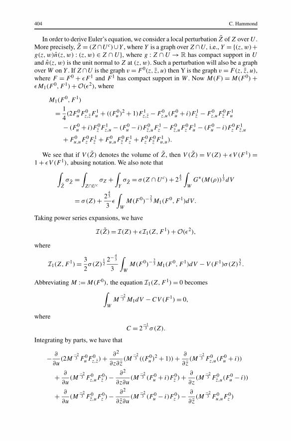
In order to derive Euler’s equation, we consider a local perturbation Z of Z over U .More precisely, Z = (Z∩Uc)∪Y , where Y is a graph over Z∩U, i.e., Y = {(z,w)+g(z,w)n(z,w) : (z,w) ∈ Z ∩ U}, where g : Z ∩ U → R has compact support in U
and n(z,w) is the unit normal to Z at (z,w). Such a perturbation will also be a graphover W on Y . If Z∩U is the graph v = F 0(z, z, u) then Y is the graph v = F(z, z, u),where F = F 0 + εF 1 and F 1 has compact support in W . Now M(F) = M(F 0) +εM1(F
0,F 1) + O(ε2), where
M1(F0,F 1)
= 1
4(2F 0
u F 0z,zF
1u + ((F 0
u )2 + 1)F 1z,z − F 0
z,u(F0u + i)F 1
z − F 0z,uF
0z F 1
u
− (F 0u + i)F 0
z F 1z,u − (F 0
u − i)F 0z,uF
1z − F 0
z,uF0z F 1
u − (F 0u − i)F 0
z F 1z,u
+ F 0u,uF
0z F 1
z + F 0u,uF
0z F 1
z + F 0z F 0
z F 1u,u).
We see that if V (Z) denotes the volume of Z, then V (Z) = V (Z) + εV (F 1) =1 + εV (F 1), abusing notation. We also note that
∫Z
σZ
=∫
Z∩Uc
σZ +∫
Y
σZ
= σ(Z ∩ Uc) + 243
∫W
G∗(M(ρ))13 dV
= σ(Z) + 243
3ε
∫W
M(F 0)−23 M1(F
0,F 1)dV .
Taking power series expansions, we have
I(Z) = I(Z) + εI1(Z,F 1) + O(ε2),
where
I1(Z,F 1) = 3
2σ(Z)
12
2− 43
3
∫W
M(F 0)−23 M1(F
0,F 1)dV − V (F 1)σ (Z)32 .
Abbreviating M := M(F 0), the equation I1(Z,F 1) = 0 becomes∫
W
M−23 M1dV − CV (F 1) = 0,
where
C = 2−13 σ(Z).
Integrating by parts, we have that
− ∂
∂u(2M
−23 F 0
u F 0z,z) + ∂2
∂z∂z(M
−23 ((F 0
u )2 + 1)) + ∂
∂z(M
−23 F 0
z,u(F0u + i))
+ ∂
∂u(M
−23 F 0
z,uF0z ) − ∂2
∂z∂u(M
−23 (F 0
u + i)F 0z ) + ∂
∂z(M
−23 F 0
z,u(F0u − i))
+ ∂
∂u(M
−23 F 0
z,uF0z ) − ∂2
∂z∂u(M
−23 (F 0
u − i)F 0z ) − ∂
∂z(M
−23 F 0
u,uF0z )
Variational Problems for Fefferman Measure 405
− ∂
∂z(M
−23 F 0
u,uF0z ) + ∂2
∂u∂u(M
−23 F 0
z F 0z ) + 4C = 0.
Note that
ρz = Fz, ρz = Fz, ρw = 1
2(Fu + i), ρw = 1
2(Fu − i),
ρw,w = 1
4Fu,u, ρz,z = Fz,z, ρz,w = 1
2Fz,u, ρz,w = 1
2Fz,u,
so that the preceding equation is equivalent to:
− ∂
∂w(M
−23 ρz,zρw) − ∂
∂w(M
−23 ρz,zρw) + ∂2
∂z∂z(M
−23 ρwρw) + ∂
∂z(M
−23 ρz,wρw)
+ ∂
∂w(M
−23 ρz,wρz) − ∂2
∂z∂w(M
−23 ρwρz) + ∂
∂z(M
−23 ρz,wρw)
+ ∂
∂w(M
−23 ρz,wρz) − ∂2
∂z∂w(M
−23 ρwρz) − ∂
∂z(M
−23 ρw,wρz)
− ∂
∂z(M
−23 ρw,wρz) + ∂2
∂w∂w(M
−23 ρzρz) + C = 0,
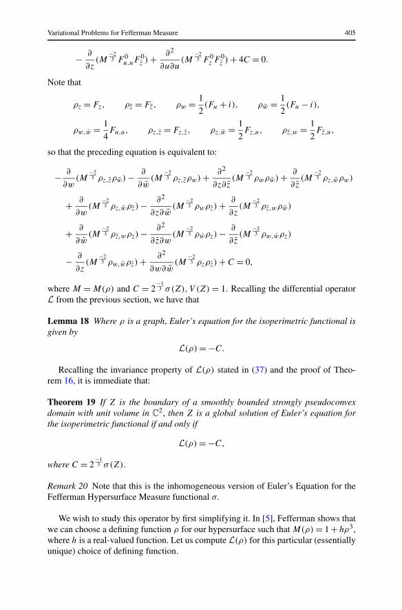
where M = M(ρ) and C = 2−13 σ(Z),V (Z) = 1. Recalling the differential operator
L from the previous section, we have that
Lemma 18 Where ρ is a graph, Euler’s equation for the isoperimetric functional isgiven by
L(ρ) = −C.
Recalling the invariance property of L(ρ) stated in (37) and the proof of Theo-rem 16, it is immediate that:
Theorem 19 If Z is the boundary of a smoothly bounded strongly pseudoconvexdomain with unit volume in C
2, then Z is a global solution of Euler’s equation forthe isoperimetric functional if and only if
L(ρ) = −C,
where C = 2−13 σ(Z).
Remark 20 Note that this is the inhomogeneous version of Euler’s Equation for theFefferman Hypersurface Measure functional σ.
We wish to study this operator by first simplifying it. In [5], Fefferman shows thatwe can choose a defining function ρ for our hypersurface such that M(ρ) = 1 + hρ3,where h is a real-valued function. Let us compute L(ρ) for this particular (essentiallyunique) choice of defining function.

406 C. Hammond
Our expression reduces to
L(ρ) = − ∂
∂w(ρz,zρw) − ∂
∂w(ρz,zρw) + ∂2
∂z∂z(ρwρw) + ∂
∂z(ρz,wρw)
+ ∂
∂w(ρz,wρz) − ∂2
∂z∂w(ρwρz) + ∂
∂z(ρz,wρw) + ∂
∂w(ρz,wρz)
− ∂2
∂z∂w(ρwρz) − ∂
∂z(ρw,wρz) − ∂
∂z(ρw,wρz) + ∂2
∂w∂w(ρzρz) + O(ρ)
= 6(ρz,wρz,w − ρz,zρw,w) + O(ρ).
The last equality above is merely computation. Therefore, we can find a definingfunction for our hypersurface so that L(ρ) = 6(ρz,wρz,w − ρz,zρw,w) on our hyper-surface. By our earlier computations (32) and (33), L(ρ) is an absolute invariant withrespect to volume-preserving biholomorphisms. Actually, this is a special case of amore general result. Namely, the Euler-Lagrange equation associated with a varia-tional problem is invariant under transformations under which the variational prob-lem is invariant. This is a nontrivial result that can be found in Olver [14]. Note thatfor the same choice of defining function, our expression for R
1,11,1 reduces to
R1,11,1 = 2
13 3(ρz,wρz,w − ρz,zρw,w).
Since neither R1,11,1 nor L(ρ) depends on the choice of defining function, we have that
L(ρ) = 223 R
1,11,1 .
The above relationship tells us that L(ρ) is also a multiple of the invariant κ .However, as we could have used κ to relate L(ρ) and R
1,11,1 , let us now also derive the
relationship between L(ρ) and the invariant κ .Suppose that our defining function is in normal form, so
ρ(z, z,w, w)
= −w − w
2i+ |z|2 + κ|z|4 + γ z3z + γ zz3
+ R(u3, zu2, zu2, u4, zu3, zu3, z2u2, z2u2, |z|2u2, z3u, z3u, z2zu, zz2u).
Here we have ignored any term that is not in the 4-jet, since this will not appear inour expression evaluated at the origin. Then
M(ρ) = 1
4(1 + 4κ|z|2 + 3γ z2 + 3γ z2)
+ R(u2, zu, zu, |z|2u, zu2, zu2, z2u, z2u, z3, z3, z2z, zz2, |z|2u2, z2zu,
zz2u, z3z, zz3, |z|4).

Variational Problems for Fefferman Measure 407
Also note that
Mz = κz + 3
2γ z + R(u, zu, zu,u2, z2, z2, |z|2)
and
Mw = R(u, z, z, |z|2, zu, zu, |z|2, z2, z2).
Now, recall that
L(ρ) = − ∂
∂w(M
−23 ρz,zρw) − ∂
∂w(M
−23 ρz,zρw) + ∂2
∂z∂z(M
−23 ρwρw)
+ ∂
∂z(M
−23 ρz,wρw) + ∂
∂w(M
−23 ρz,wρz) − ∂2
∂z∂w(M
−23 ρwρz)
+ ∂
∂z(M
−23 ρz,wρw) + ∂
∂w(M
−23 ρz,wρz) − ∂2
∂z∂w(M
−23 ρwρz)
− ∂
∂z(M
−23 ρw,wρz) − ∂
∂z(M
−23 ρw,wρz) + ∂2
∂w∂w(M
−23 ρzρz).
By our earlier observation, any term that is multiplied by a first-order derivative of
M−23 may be discarded. Likewise, any term multiplying ρz or ρz. Moreover, since
ρw = −1
2i+ R(u2, zu, zu,u3, zu2, zu2, z2u, z2u, |z|2u, z3, z3, z2z, zz2),
we see that any term multiplying ρz,w,z, ρz,w,z, ρz,w,z, ρz,w,z, ρz,w,z, ρz,w,z may bediscarded. Likewise, any term multiplying ρw,w, ρw,w,ρw,w may be discarded. Im-
plementing all of these simplifications, we find M23 L(ρ) = −2
3 M−1|ρw|2Mz,z +R(z, z, u). Since Mz,z = κ + R(z, z, u), we find that at the origin,
L(ρ) = −273
3κ. (38)
For a sphere of radius R, ρ = zz + ww − R2. We have V (Z) = π2
2 R4 and s(Z) =2π2R3 are the volume and surface area, respectively. Now, |∇ρ| = 2R and M(ρ) =R2, so σZ = 2
43 R− 1
3 sZ, which implies that the Fefferman measure of the sphere is
merely σ(Z) = 243 R− 1
3 s(Z) = 243 2π2R
83 . For the sphere of radius R,
L(ρ) = −4R−43 .
If we assume the sphere has unit volume, V = 1, then R4 = 2π2 . We merely check
that the left- and right-hand sides are equal. Since L(ρ) = 223 R
1,11,1 , we immediately
obtain the following:
Theorem 21 Let Z ⊂ C2 be a strongly pseudoconvex, four times continuously dif-ferentiable real hypersurface bounding a domain with unit volume. Then Z is a

408 C. Hammond
global solution of Euler’s equation for the isoperimetric functional if and only ifR
1,11,1 = − 1
2σ(Z) on Z.
Which, by Theorem 7, gives:
Corollary 22 A torsion-free strongly pseudoconvex real-analytic, real hypersurfaceZ ⊂ C
2 bounding a domain with unit volume is a global solution of Euler’s equationfor the isoperimetric functional if and only if Z is locally the image of a sphere undera volume-preserving holomorphic map.
We also have the following:
Theorem 23 Let Z ⊂ C2 be a strongly pseudoconvex, four times continuously dif-
ferentiable real hypersurface. Then Z satisfies the Euler equation for the extremalhypersurface problem if and only if R
1,11,1 = 0 on Z.
Remark 24 There are several interesting questions that remain here. We would liketo analyze the second variation of the Isoperimetric Functional. It is already clearthat spheres are not minima for the Isoperimetric Functional but rather saddle points.However, Barrett has shown that if one restricts to a special class of hypersurfaces,that changes. In particular, he has obtained an Isoperimetric Inequality for completecircular domains.
We would also like to determine whether or not the spheres are the only compact,simply connected hypersurfaces having constant holomorphic sectional curvature.
References
1. Baouendi, S., Ebenfelt, P., Rothschild, L.: Real Submanifolds in Complex Spaces and their Mappings.Princeton University Press, Princeton (1999)
2. Barrett, D.: A floating body approach to Fefferman’s hypersurface measure. Math. Scand. 98, 69–80(2006)
3. Burns, D. Jr., Shnider, S.: Real hypersurfaces in complex manifolds. In: Several Complex Variables,Proc. Symposium Pure Math., Vol. XXX, Part 2, Williams Coll., Williamstown, Mass., 1975, pp.141–168. American Math. Society, Providence (1977)
4. Chern, S.S., Moser, J.K.: Real hypersurfaces in complex manifolds. Acta Math. 133, 219–271 (1974)5. Fefferman, C.: Parabolic invariant theory in complex analysis. Adv. Math. 31, 131–262 (1979)6. Fels, M., Olver, P.J.: Moving frames II: regularization and theoretical foundations. Acta Appl. Math.
55, 127–208 (1999)7. Fomin, S.V., Gelfand, I.M.: Calculus of Variations. Prentice Hall, Englewood Cliffs (1963)8. Forstneric, F.: Interpolation by Holomorphic Automorphisms and Embeddings in C
n . J. Geom. Anal.9, 93–117 (1999)
9. Ivey, T.A., Landsberg, J.M.: Cartan for Beginners: Differential Geometry via Moving Frames andExterior Differential Systems. American Math. Society, Providence (2003)
10. Jensen, G.R.: Higher Order Contact of Submanifolds of Homogeneous Spaces. Springer, New York(1977)
11. Kobayashi, S., Nomizu, K.: Foundations of Differential Geometry, vol. I. Wiley, New York (1963)12. Nomizu, K., Sasaki, T.: Affine Differential Geometry. Cambridge University Press, New York (1994)13. Olver, P.J.: Differential invariants of surfaces. Differ. Geom. Appl. (to appear)14. Olver, P.J.: Equivalence, Invariants, and Symmetry. Cambridge University Press, New York (1995)15. Tanaka, N.: On the pseudo-conformal geometry of hypersurfaces of the space of n complex variables.
J. Math. Soc. Jpn. 14, 397–429 (1962)16. Webster, S.M.: Pseudo-Hermitian structures on a real hypersurface. J. Differ. Geom. 13, 25–41 (1978)