Hypersurface singularity in arbitrary characteristic · Hypersurface singularity in arbitrary...
148
Hypersurface singularity in arbitrary characteristic Rodrigo Salom˜ ao (UFF) 24 th Brazilian Algebra Meeting 02 August, 2016 Joint work with Abramo Hefez and Jo˜ ao H´ elder Olmedo Rodrigues (UFF) Rodrigo Salom˜ ao (UFF) 24 th Brazilian Algebra Meeting 1 / 24
Transcript of Hypersurface singularity in arbitrary characteristic · Hypersurface singularity in arbitrary...
Hypersurface singularity in arbitrarycharacteristic
Rodrigo Salomao (UFF)
24th Brazilian Algebra Meeting
02 August, 2016
Joint work withAbramo Hefez and Joao Helder Olmedo Rodrigues
(UFF)
Rodrigo Salomao (UFF) 24th Brazilian Algebra Meeting 1 / 24

Introduction
Let us consider k be an algebraically closed field with p = char(k) ≥ 0 and
SpecO be a singular algebroid hypersurface over k, that is,
O ' R/A
where
R = k[[X1, . . . ,Xn]] and A ⊂ R is a principal ideal.
Each generator of A is called an equation for O and we denote
Of := R/〈f 〉.
We note that
Of ' Og ⇐⇒ f ∼K g (Contact Equivalent)
f ∼K g : there is an automorphism φ of R and a unit u ∈ R∗ such thatg = u · φ(f ).
Rodrigo Salomao (UFF) 24th Brazilian Algebra Meeting 2 / 24

Introduction
Given an equation f for O, the Tjurina Ideal of f is the ideal
T (f ) = 〈f , fX1 , . . . , fXn〉 ⊂ R.
and the Tjurina Number of O is,
τ(O) = τ(f ) := dimk R/T (f ) ∈ N ∪∞
which is an invariant of O. We say that O is an isolated singularity ifτ(O) <∞.
The Jacobian Ideal of f is the ideal
J(f ) = 〈fX1 , . . . , fXn〉 ⊂ R
and the Milnor Number of f is
µ(f ) := dimk R/J(f ) ∈ N ∪∞.
Rodrigo Salomao (UFF) 24th Brazilian Algebra Meeting 3 / 24
Introduction
Given an equation f for O, the Tjurina Ideal of f is the ideal
T (f ) = 〈f , fX1 , . . . , fXn〉 ⊂ R.
and the Tjurina Number of O is,
τ(O) = τ(f ) := dimk R/T (f ) ∈ N ∪∞
which is an invariant of O.
We say that O is an isolated singularity ifτ(O) <∞.
The Jacobian Ideal of f is the ideal
J(f ) = 〈fX1 , . . . , fXn〉 ⊂ R
and the Milnor Number of f is
µ(f ) := dimk R/J(f ) ∈ N ∪∞.
Rodrigo Salomao (UFF) 24th Brazilian Algebra Meeting 3 / 24
Introduction
Given an equation f for O, the Tjurina Ideal of f is the ideal
T (f ) = 〈f , fX1 , . . . , fXn〉 ⊂ R.
and the Tjurina Number of O is,
τ(O) = τ(f ) := dimk R/T (f ) ∈ N ∪∞
which is an invariant of O. We say that O is an isolated singularity ifτ(O) <∞.
The Jacobian Ideal of f is the ideal
J(f ) = 〈fX1 , . . . , fXn〉 ⊂ R
and the Milnor Number of f is
µ(f ) := dimk R/J(f ) ∈ N ∪∞.
Rodrigo Salomao (UFF) 24th Brazilian Algebra Meeting 3 / 24
Introduction
Given an equation f for O, the Tjurina Ideal of f is the ideal
T (f ) = 〈f , fX1 , . . . , fXn〉 ⊂ R.
and the Tjurina Number of O is,
τ(O) = τ(f ) := dimk R/T (f ) ∈ N ∪∞
which is an invariant of O. We say that O is an isolated singularity ifτ(O) <∞.
The Jacobian Ideal of f is the ideal
J(f ) = 〈fX1 , . . . , fXn〉 ⊂ R
and the Milnor Number of f is
µ(f ) := dimk R/J(f ) ∈ N ∪∞.
Rodrigo Salomao (UFF) 24th Brazilian Algebra Meeting 3 / 24
Introduction
Remark:
1 J(f ) ⊆ T (f )⇒ τ(f ) 6 µ(f ).
Hence, µ(f ) <∞ ⇒ O is an isolatedsingularity.
2 If k = C then it is possible to prove that
τ(f ) <∞ ⇒ µ(f ) <∞;f ∼K g ⇒ µ(f ) = µ(g). Hence the Milnor number of any equationrepresenting O is an invariant of O.
Both properties are no longer true if char k = p > 0.
Example: If f = Y p + X p+1 ∈ k[[X ,Y ]] then τ(f ) = p2 <∞. On theother hand µ(f ) =∞, µ((1 + Y )f ) = p2 and µ((1 + Y 2)f ) = p2 + p.
Rodrigo Salomao (UFF) 24th Brazilian Algebra Meeting 4 / 24
Introduction
Remark:
1 J(f ) ⊆ T (f )⇒ τ(f ) 6 µ(f ). Hence, µ(f ) <∞ ⇒ O is an isolatedsingularity.
2 If k = C then it is possible to prove that
τ(f ) <∞ ⇒ µ(f ) <∞;
f ∼K g ⇒ µ(f ) = µ(g). Hence the Milnor number of any equationrepresenting O is an invariant of O.
Both properties are no longer true if char k = p > 0.
Example: If f = Y p + X p+1 ∈ k[[X ,Y ]] then τ(f ) = p2 <∞. On theother hand µ(f ) =∞, µ((1 + Y )f ) = p2 and µ((1 + Y 2)f ) = p2 + p.
Rodrigo Salomao (UFF) 24th Brazilian Algebra Meeting 4 / 24
Introduction
Remark:
1 J(f ) ⊆ T (f )⇒ τ(f ) 6 µ(f ). Hence, µ(f ) <∞ ⇒ O is an isolatedsingularity.
2 If k = C then it is possible to prove that
τ(f ) <∞ ⇒ µ(f ) <∞;f ∼K g ⇒ µ(f ) = µ(g).
Hence the Milnor number of any equationrepresenting O is an invariant of O.
Both properties are no longer true if char k = p > 0.
Example: If f = Y p + X p+1 ∈ k[[X ,Y ]] then τ(f ) = p2 <∞. On theother hand µ(f ) =∞, µ((1 + Y )f ) = p2 and µ((1 + Y 2)f ) = p2 + p.
Rodrigo Salomao (UFF) 24th Brazilian Algebra Meeting 4 / 24
Introduction
Remark:
1 J(f ) ⊆ T (f )⇒ τ(f ) 6 µ(f ). Hence, µ(f ) <∞ ⇒ O is an isolatedsingularity.
2 If k = C then it is possible to prove that
τ(f ) <∞ ⇒ µ(f ) <∞;f ∼K g ⇒ µ(f ) = µ(g). Hence the Milnor number of any equationrepresenting O is an invariant of O.
Both properties are no longer true if char k = p > 0.
Example: If f = Y p + X p+1 ∈ k[[X ,Y ]] then τ(f ) = p2 <∞. On theother hand µ(f ) =∞, µ((1 + Y )f ) = p2 and µ((1 + Y 2)f ) = p2 + p.
Rodrigo Salomao (UFF) 24th Brazilian Algebra Meeting 4 / 24
Introduction
Remark:
1 J(f ) ⊆ T (f )⇒ τ(f ) 6 µ(f ). Hence, µ(f ) <∞ ⇒ O is an isolatedsingularity.
2 If k = C then it is possible to prove that
τ(f ) <∞ ⇒ µ(f ) <∞;f ∼K g ⇒ µ(f ) = µ(g). Hence the Milnor number of any equationrepresenting O is an invariant of O.
Both properties are no longer true if char k = p > 0.
Example: If f = Y p + X p+1 ∈ k[[X ,Y ]] then τ(f ) = p2 <∞.
On theother hand µ(f ) =∞, µ((1 + Y )f ) = p2 and µ((1 + Y 2)f ) = p2 + p.
Rodrigo Salomao (UFF) 24th Brazilian Algebra Meeting 4 / 24
Introduction
Remark:
1 J(f ) ⊆ T (f )⇒ τ(f ) 6 µ(f ). Hence, µ(f ) <∞ ⇒ O is an isolatedsingularity.
2 If k = C then it is possible to prove that
τ(f ) <∞ ⇒ µ(f ) <∞;f ∼K g ⇒ µ(f ) = µ(g). Hence the Milnor number of any equationrepresenting O is an invariant of O.
Both properties are no longer true if char k = p > 0.
Example: If f = Y p + X p+1 ∈ k[[X ,Y ]] then τ(f ) = p2 <∞. On theother hand µ(f ) =∞,
µ((1 + Y )f ) = p2 and µ((1 + Y 2)f ) = p2 + p.
Rodrigo Salomao (UFF) 24th Brazilian Algebra Meeting 4 / 24
Introduction
Remark:
1 J(f ) ⊆ T (f )⇒ τ(f ) 6 µ(f ). Hence, µ(f ) <∞ ⇒ O is an isolatedsingularity.
2 If k = C then it is possible to prove that
τ(f ) <∞ ⇒ µ(f ) <∞;f ∼K g ⇒ µ(f ) = µ(g). Hence the Milnor number of any equationrepresenting O is an invariant of O.
Both properties are no longer true if char k = p > 0.
Example: If f = Y p + X p+1 ∈ k[[X ,Y ]] then τ(f ) = p2 <∞. On theother hand µ(f ) =∞, µ((1 + Y )f ) = p2
and µ((1 + Y 2)f ) = p2 + p.
Rodrigo Salomao (UFF) 24th Brazilian Algebra Meeting 4 / 24
Introduction
Remark:
1 J(f ) ⊆ T (f )⇒ τ(f ) 6 µ(f ). Hence, µ(f ) <∞ ⇒ O is an isolatedsingularity.
2 If k = C then it is possible to prove that
τ(f ) <∞ ⇒ µ(f ) <∞;f ∼K g ⇒ µ(f ) = µ(g). Hence the Milnor number of any equationrepresenting O is an invariant of O.
Both properties are no longer true if char k = p > 0.
Example: If f = Y p + X p+1 ∈ k[[X ,Y ]] then τ(f ) = p2 <∞. On theother hand µ(f ) =∞, µ((1 + Y )f ) = p2 and µ((1 + Y 2)f ) = p2 + p.
Rodrigo Salomao (UFF) 24th Brazilian Algebra Meeting 4 / 24

Finiteness of µ
Question: For which f do we have µ(f ) <∞?
Proposition. If f ∈ m ⊂ R and τ(f ) <∞, then
µ(f ) <∞ ⇐⇒ f ∈√J(f ).
(Teissier, 1972) p = 0 =⇒ f ∈ J(f ) ⊆√J(f ).
Therefore, p = 0 and τ(f ) <∞ =⇒ µ(f ) <∞.
Rodrigo Salomao (UFF) 24th Brazilian Algebra Meeting 5 / 24
Finiteness of µ
Question: For which f do we have µ(f ) <∞?
Proposition. If f ∈ m ⊂ R and τ(f ) <∞, then
µ(f ) <∞ ⇐⇒ f ∈√
J(f ).
(Teissier, 1972) p = 0 =⇒ f ∈ J(f ) ⊆√J(f ).
Therefore, p = 0 and τ(f ) <∞ =⇒ µ(f ) <∞.
Rodrigo Salomao (UFF) 24th Brazilian Algebra Meeting 5 / 24
Finiteness of µ
Question: For which f do we have µ(f ) <∞?
Proposition. If f ∈ m ⊂ R and τ(f ) <∞, then
µ(f ) <∞ ⇐⇒ f ∈√
J(f ).
(Teissier, 1972) p = 0 =⇒ f ∈ J(f ) ⊆√
J(f ).
Therefore, p = 0 and τ(f ) <∞ =⇒ µ(f ) <∞.
Rodrigo Salomao (UFF) 24th Brazilian Algebra Meeting 5 / 24
Finiteness of µ
Question: For which f do we have µ(f ) <∞?
Proposition. If f ∈ m ⊂ R and τ(f ) <∞, then
µ(f ) <∞ ⇐⇒ f ∈√
J(f ).
(Teissier, 1972) p = 0 =⇒ f ∈ J(f ) ⊆√
J(f ).
Therefore, p = 0 and τ(f ) <∞ =⇒ µ(f ) <∞.
Rodrigo Salomao (UFF) 24th Brazilian Algebra Meeting 5 / 24
Connection with Bertini’s Theorem
Let us consider f ∈ k[X1, · · · ,Xn] and Z (f ) with an isolated singularity inthe origin 0 ∈ An
k
, that is,
0 ∈ Sing(Z (f )) and τ0(f ) := dimk
OAnk ,0
T (f )= τ(f ) <∞.
There is a natural map of evaluation f : Ank → A1
k , which is a fibration byhypersurfaces;
If p = 0, it follows from Bertini’s Theorem on variation of singular pointsthat there are neighborhoods U of 0 ∈ An
k and V of 0 ∈ A1k such that
U \ f −1(0) −→ V \ 0
is smooth. In this case we say that the evaluation map is a localsmoothing of the singularity 0 ∈ Z (f ).
Rodrigo Salomao (UFF) 24th Brazilian Algebra Meeting 6 / 24
Connection with Bertini’s Theorem
Let us consider f ∈ k[X1, · · · ,Xn] and Z (f ) with an isolated singularity inthe origin 0 ∈ An
k , that is,
0 ∈ Sing(Z (f )) and τ0(f ) := dimk
OAnk ,0
T (f )= τ(f ) <∞.
There is a natural map of evaluation f : Ank → A1
k , which is a fibration byhypersurfaces;
If p = 0
, it follows from Bertini’s Theorem on variation of singular pointsthat there are neighborhoods U of 0 ∈ An
k and V of 0 ∈ A1k such that
U \ f −1(0) −→ V \ 0
is smooth. In this case we say that the evaluation map is a localsmoothing of the singularity 0 ∈ Z (f ).
Rodrigo Salomao (UFF) 24th Brazilian Algebra Meeting 6 / 24
Connection with Bertini’s Theorem
Let us consider f ∈ k[X1, · · · ,Xn] and Z (f ) with an isolated singularity inthe origin 0 ∈ An
k , that is,
0 ∈ Sing(Z (f )) and τ0(f ) := dimk
OAnk ,0
T (f )= τ(f ) <∞.
There is a natural map of evaluation f : Ank → A1
k , which is a fibration byhypersurfaces;
If p = 0, it follows from Bertini’s Theorem on variation of singular pointsthat
there are neighborhoods U of 0 ∈ Ank and V of 0 ∈ A1
k such that
U \ f −1(0) −→ V \ 0
is smooth. In this case we say that the evaluation map is a localsmoothing of the singularity 0 ∈ Z (f ).
Rodrigo Salomao (UFF) 24th Brazilian Algebra Meeting 6 / 24
Connection with Bertini’s Theorem
Let us consider f ∈ k[X1, · · · ,Xn] and Z (f ) with an isolated singularity inthe origin 0 ∈ An
k , that is,
0 ∈ Sing(Z (f )) and τ0(f ) := dimk
OAnk ,0
T (f )= τ(f ) <∞.
There is a natural map of evaluation f : Ank → A1
k , which is a fibration byhypersurfaces;
If p = 0, it follows from Bertini’s Theorem on variation of singular pointsthat there are neighborhoods U of 0 ∈ An
k and V of 0 ∈ A1k such that
U \ f −1(0) −→ V \ 0
is smooth.
In this case we say that the evaluation map is a localsmoothing of the singularity 0 ∈ Z (f ).
Rodrigo Salomao (UFF) 24th Brazilian Algebra Meeting 6 / 24
Connection with Bertini’s Theorem
Let us consider f ∈ k[X1, · · · ,Xn] and Z (f ) with an isolated singularity inthe origin 0 ∈ An
k , that is,
0 ∈ Sing(Z (f )) and τ0(f ) := dimk
OAnk ,0
T (f )= τ(f ) <∞.
There is a natural map of evaluation f : Ank → A1
k , which is a fibration byhypersurfaces;
If p = 0, it follows from Bertini’s Theorem on variation of singular pointsthat there are neighborhoods U of 0 ∈ An
k and V of 0 ∈ A1k such that
U \ f −1(0) −→ V \ 0
is smooth. In this case we say that the evaluation map is a localsmoothing of the singularity 0 ∈ Z (f ).
Rodrigo Salomao (UFF) 24th Brazilian Algebra Meeting 6 / 24
Connection with Bertini’s Theorem
As was discovered by Zariski, the above Bertini’s Theorem does not workanymore if p > 0.
Example: f = Y p − X p+1, τ0(f ) = p2 <∞. For each s ∈ A1k ,
Sing(f −1(s)
)= {(0, s1/p)}.
Question: When f : Ank → A1
k is a local smoothing of the singularity0 ∈ Z (f ) = f −1(0)?
Theorem. Let f ∈ k[X1, · · · ,Xn] admitting an isolated singularity at theorigin of An
k . The fibration f : Ank → A1
k is a local smoothing at
0 ∈ f −1(0) if and only if µ0(f ) := dimk
OAnk,0
J(f ) = µ(f ) <∞.
Rodrigo Salomao (UFF) 24th Brazilian Algebra Meeting 7 / 24
Connection with Bertini’s Theorem
As was discovered by Zariski, the above Bertini’s Theorem does not workanymore if p > 0.
Example: f = Y p − X p+1,
τ0(f ) = p2 <∞. For each s ∈ A1k ,
Sing(f −1(s)
)= {(0, s1/p)}.
Question: When f : Ank → A1
k is a local smoothing of the singularity0 ∈ Z (f ) = f −1(0)?
Theorem. Let f ∈ k[X1, · · · ,Xn] admitting an isolated singularity at theorigin of An
k . The fibration f : Ank → A1
k is a local smoothing at
0 ∈ f −1(0) if and only if µ0(f ) := dimk
OAnk,0
J(f ) = µ(f ) <∞.
Rodrigo Salomao (UFF) 24th Brazilian Algebra Meeting 7 / 24
Connection with Bertini’s Theorem
As was discovered by Zariski, the above Bertini’s Theorem does not workanymore if p > 0.
Example: f = Y p − X p+1, τ0(f ) = p2 <∞.
For each s ∈ A1k ,
Sing(f −1(s)
)= {(0, s1/p)}.
Question: When f : Ank → A1
k is a local smoothing of the singularity0 ∈ Z (f ) = f −1(0)?
Theorem. Let f ∈ k[X1, · · · ,Xn] admitting an isolated singularity at theorigin of An
k . The fibration f : Ank → A1
k is a local smoothing at
0 ∈ f −1(0) if and only if µ0(f ) := dimk
OAnk,0
J(f ) = µ(f ) <∞.
Rodrigo Salomao (UFF) 24th Brazilian Algebra Meeting 7 / 24
Connection with Bertini’s Theorem
As was discovered by Zariski, the above Bertini’s Theorem does not workanymore if p > 0.
Example: f = Y p − X p+1, τ0(f ) = p2 <∞. For each s ∈ A1k ,
Sing(f −1(s)
)= {(0, s1/p)}.
Question: When f : Ank → A1
k is a local smoothing of the singularity0 ∈ Z (f ) = f −1(0)?
Theorem. Let f ∈ k[X1, · · · ,Xn] admitting an isolated singularity at theorigin of An
k . The fibration f : Ank → A1
k is a local smoothing at
0 ∈ f −1(0) if and only if µ0(f ) := dimk
OAnk,0
J(f ) = µ(f ) <∞.
Rodrigo Salomao (UFF) 24th Brazilian Algebra Meeting 7 / 24
Connection with Bertini’s Theorem
As was discovered by Zariski, the above Bertini’s Theorem does not workanymore if p > 0.
Example: f = Y p − X p+1, τ0(f ) = p2 <∞. For each s ∈ A1k ,
Sing(f −1(s)
)= {(0, s1/p)}.
Question: When f : Ank → A1
k is a local smoothing of the singularity0 ∈ Z (f ) = f −1(0)?
Theorem. Let f ∈ k[X1, · · · ,Xn] admitting an isolated singularity at theorigin of An
k . The fibration f : Ank → A1
k is a local smoothing at
0 ∈ f −1(0) if and only if µ0(f ) := dimk
OAnk,0
J(f ) = µ(f ) <∞.
Rodrigo Salomao (UFF) 24th Brazilian Algebra Meeting 7 / 24
Connection with vector fields
f ∈ R = k[[X ,Y ]] reduced (⇔ Of has an isolated singularity)
char k = p > 0
φ(f ) ∈ k[[X ,Y p]] for some automorphism φ of R =⇒ µ(f ) =∞.
Question: Is the converse true?
Remark: f ∈ k[[X ,Y p]] = Ker( ∂∂Y )⇐⇒ Df := fY
∂∂X − fX
∂∂Y =h ∂
∂Y ,
with h ∈ k[[X ,Y ]]. In this case we say that Df and ∂∂Y are equivalent
vector fields and we write Df ∼ ∂∂Y .
Rodrigo Salomao (UFF) 24th Brazilian Algebra Meeting 8 / 24
Connection with vector fields
f ∈ R = k[[X ,Y ]] reduced (⇔ Of has an isolated singularity)
char k = p > 0
φ(f ) ∈ k[[X ,Y p]] for some automorphism φ of R =⇒ µ(f ) =∞.
Question: Is the converse true?
Remark: f ∈ k[[X ,Y p]] = Ker( ∂∂Y )⇐⇒ Df := fY
∂∂X − fX
∂∂Y =
h ∂∂Y ,
with h ∈ k[[X ,Y ]]. In this case we say that Df and ∂∂Y are equivalent
vector fields and we write Df ∼ ∂∂Y .
Rodrigo Salomao (UFF) 24th Brazilian Algebra Meeting 8 / 24
Connection with vector fields
f ∈ R = k[[X ,Y ]] reduced (⇔ Of has an isolated singularity)
char k = p > 0
φ(f ) ∈ k[[X ,Y p]] for some automorphism φ of R =⇒ µ(f ) =∞.
Question: Is the converse true?
Remark: f ∈ k[[X ,Y p]] = Ker( ∂∂Y )⇐⇒ Df := fY
∂∂X − fX
∂∂Y =h ∂
∂Y ,
with h ∈ k[[X ,Y ]].
In this case we say that Df and ∂∂Y are equivalent
vector fields and we write Df ∼ ∂∂Y .
Rodrigo Salomao (UFF) 24th Brazilian Algebra Meeting 8 / 24
Connection with vector fields
f ∈ R = k[[X ,Y ]] reduced (⇔ Of has an isolated singularity)
char k = p > 0
φ(f ) ∈ k[[X ,Y p]] for some automorphism φ of R =⇒ µ(f ) =∞.
Question: Is the converse true?
Remark: f ∈ k[[X ,Y p]] = Ker( ∂∂Y )⇐⇒ Df := fY
∂∂X − fX
∂∂Y =h ∂
∂Y ,
with h ∈ k[[X ,Y ]]. In this case we say that Df and ∂∂Y are equivalent
vector fields and we write Df ∼ ∂∂Y .
Rodrigo Salomao (UFF) 24th Brazilian Algebra Meeting 8 / 24
Connection with vector fields
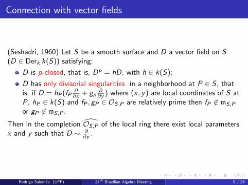
(Seshadri, 1960) Let S be a smooth surface and D a vector field on S
(D ∈ Derk k(S)) satisfying:
D is p-closed, that is, Dp = hD, with h ∈ k(S);
D has only divisorial singularities in a neighborhood at P ∈ S , thatis, if D = hP(fP
∂∂x + gp
∂∂y ) where (x , y) are local coordinates of S at
P, hP ∈ k(S) and fP , gP ∈ OS,P are relatively prime then fP 6∈ mS ,P
or gP 6∈ mS,P .
Then in the completion OS,P of the local ring there exist local parametersx and y such that D ∼ ∂
∂y .
Rodrigo Salomao (UFF) 24th Brazilian Algebra Meeting 9 / 24
Connection with vector fields
(Seshadri, 1960) Let S be a smooth surface and D a vector field on S(D ∈ Derk k(S))
satisfying:
D is p-closed, that is, Dp = hD, with h ∈ k(S);
D has only divisorial singularities in a neighborhood at P ∈ S , thatis, if D = hP(fP
∂∂x + gp
∂∂y ) where (x , y) are local coordinates of S at
P, hP ∈ k(S) and fP , gP ∈ OS,P are relatively prime then fP 6∈ mS ,P
or gP 6∈ mS,P .
Then in the completion OS,P of the local ring there exist local parametersx and y such that D ∼ ∂
∂y .
Rodrigo Salomao (UFF) 24th Brazilian Algebra Meeting 9 / 24
Connection with vector fields
(Seshadri, 1960) Let S be a smooth surface and D a vector field on S(D ∈ Derk k(S)) satisfying:
D is p-closed,
that is, Dp = hD, with h ∈ k(S);
D has only divisorial singularities in a neighborhood at P ∈ S , thatis, if D = hP(fP
∂∂x + gp
∂∂y ) where (x , y) are local coordinates of S at
P, hP ∈ k(S) and fP , gP ∈ OS,P are relatively prime then fP 6∈ mS ,P
or gP 6∈ mS,P .
Then in the completion OS,P of the local ring there exist local parametersx and y such that D ∼ ∂
∂y .
Rodrigo Salomao (UFF) 24th Brazilian Algebra Meeting 9 / 24
Connection with vector fields
(Seshadri, 1960) Let S be a smooth surface and D a vector field on S(D ∈ Derk k(S)) satisfying:
D is p-closed, that is, Dp = hD, with h ∈ k(S);
D has only divisorial singularities in a neighborhood at P ∈ S , thatis, if D = hP(fP
∂∂x + gp
∂∂y ) where (x , y) are local coordinates of S at
P, hP ∈ k(S) and fP , gP ∈ OS,P are relatively prime then fP 6∈ mS ,P
or gP 6∈ mS,P .
Then in the completion OS,P of the local ring there exist local parametersx and y such that D ∼ ∂
∂y .
Rodrigo Salomao (UFF) 24th Brazilian Algebra Meeting 9 / 24
Connection with vector fields
(Seshadri, 1960) Let S be a smooth surface and D a vector field on S(D ∈ Derk k(S)) satisfying:
D is p-closed, that is, Dp = hD, with h ∈ k(S);
D has only divisorial singularities in a neighborhood at P ∈ S ,
thatis, if D = hP(fP
∂∂x + gp
∂∂y ) where (x , y) are local coordinates of S at
P, hP ∈ k(S) and fP , gP ∈ OS,P are relatively prime then fP 6∈ mS ,P
or gP 6∈ mS,P .
Then in the completion OS,P of the local ring there exist local parametersx and y such that D ∼ ∂
∂y .
Rodrigo Salomao (UFF) 24th Brazilian Algebra Meeting 9 / 24
Connection with vector fields
(Seshadri, 1960) Let S be a smooth surface and D a vector field on S(D ∈ Derk k(S)) satisfying:
D is p-closed, that is, Dp = hD, with h ∈ k(S);
D has only divisorial singularities in a neighborhood at P ∈ S , thatis, if D = hP(fP
∂∂x + gp
∂∂y ) where (x , y) are local coordinates of S at
P,
hP ∈ k(S) and fP , gP ∈ OS,P are relatively prime then fP 6∈ mS ,P
or gP 6∈ mS,P .
Then in the completion OS,P of the local ring there exist local parametersx and y such that D ∼ ∂
∂y .
Rodrigo Salomao (UFF) 24th Brazilian Algebra Meeting 9 / 24
Connection with vector fields
(Seshadri, 1960) Let S be a smooth surface and D a vector field on S(D ∈ Derk k(S)) satisfying:
D is p-closed, that is, Dp = hD, with h ∈ k(S);
D has only divisorial singularities in a neighborhood at P ∈ S , thatis, if D = hP(fP
∂∂x + gp
∂∂y ) where (x , y) are local coordinates of S at
P, hP ∈ k(S) and fP , gP ∈ OS,P are relatively prime
then fP 6∈ mS ,P
or gP 6∈ mS,P .
Then in the completion OS,P of the local ring there exist local parametersx and y such that D ∼ ∂
∂y .
Rodrigo Salomao (UFF) 24th Brazilian Algebra Meeting 9 / 24
Connection with vector fields
(Seshadri, 1960) Let S be a smooth surface and D a vector field on S(D ∈ Derk k(S)) satisfying:
D is p-closed, that is, Dp = hD, with h ∈ k(S);
D has only divisorial singularities in a neighborhood at P ∈ S , thatis, if D = hP(fP
∂∂x + gp
∂∂y ) where (x , y) are local coordinates of S at
P, hP ∈ k(S) and fP , gP ∈ OS,P are relatively prime then fP 6∈ mS ,P
or gP 6∈ mS,P .
Then in the completion OS,P of the local ring there exist local parametersx and y such that D ∼ ∂
∂y .
Rodrigo Salomao (UFF) 24th Brazilian Algebra Meeting 9 / 24
Connection with vector fields
(Seshadri, 1960) Let S be a smooth surface and D a vector field on S(D ∈ Derk k(S)) satisfying:
D is p-closed, that is, Dp = hD, with h ∈ k(S);
D has only divisorial singularities in a neighborhood at P ∈ S , thatis, if D = hP(fP
∂∂x + gp
∂∂y ) where (x , y) are local coordinates of S at
P, hP ∈ k(S) and fP , gP ∈ OS,P are relatively prime then fP 6∈ mS ,P
or gP 6∈ mS,P .
Then in the completion OS,P of the local ring there exist local parametersx and y such that D ∼ ∂
∂y .
Rodrigo Salomao (UFF) 24th Brazilian Algebra Meeting 9 / 24
Connection with vector fields
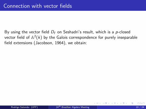
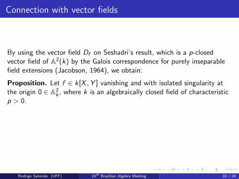
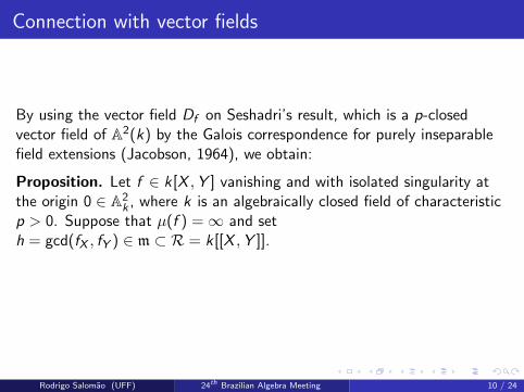
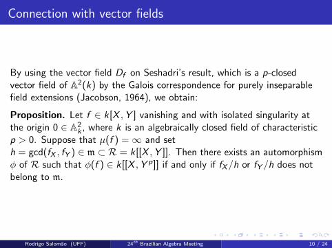
By using the vector field Df on Seshadri’s result, which is a p-closedvector field of A2(k) by the Galois correspondence for purely inseparablefield extensions (Jacobson, 1964), we obtain:
Proposition. Let f ∈ k[X ,Y ] vanishing and with isolated singularity atthe origin 0 ∈ A2
k , where k is an algebraically closed field of characteristicp > 0. Suppose that µ(f ) =∞ and seth = gcd(fX , fY ) ∈ m ⊂ R = k[[X ,Y ]]. Then there exists an automorphismφ of R such that φ(f ) ∈ k[[X ,Y p]] if and only if fX/h or fY /h does notbelong to m.
Rodrigo Salomao (UFF) 24th Brazilian Algebra Meeting 10 / 24
Connection with vector fields
By using the vector field Df on Seshadri’s result, which is a p-closedvector field of A2(k) by the Galois correspondence for purely inseparablefield extensions (Jacobson, 1964), we obtain:
Proposition. Let f ∈ k[X ,Y ] vanishing and with isolated singularity atthe origin 0 ∈ A2
k , where k is an algebraically closed field of characteristicp > 0.
Suppose that µ(f ) =∞ and seth = gcd(fX , fY ) ∈ m ⊂ R = k[[X ,Y ]]. Then there exists an automorphismφ of R such that φ(f ) ∈ k[[X ,Y p]] if and only if fX/h or fY /h does notbelong to m.
Rodrigo Salomao (UFF) 24th Brazilian Algebra Meeting 10 / 24
Connection with vector fields
By using the vector field Df on Seshadri’s result, which is a p-closedvector field of A2(k) by the Galois correspondence for purely inseparablefield extensions (Jacobson, 1964), we obtain:
Proposition. Let f ∈ k[X ,Y ] vanishing and with isolated singularity atthe origin 0 ∈ A2
k , where k is an algebraically closed field of characteristicp > 0. Suppose that µ(f ) =∞ and seth = gcd(fX , fY ) ∈ m ⊂ R = k[[X ,Y ]].
Then there exists an automorphismφ of R such that φ(f ) ∈ k[[X ,Y p]] if and only if fX/h or fY /h does notbelong to m.
Rodrigo Salomao (UFF) 24th Brazilian Algebra Meeting 10 / 24
Connection with vector fields
By using the vector field Df on Seshadri’s result, which is a p-closedvector field of A2(k) by the Galois correspondence for purely inseparablefield extensions (Jacobson, 1964), we obtain:
Proposition. Let f ∈ k[X ,Y ] vanishing and with isolated singularity atthe origin 0 ∈ A2
k , where k is an algebraically closed field of characteristicp > 0. Suppose that µ(f ) =∞ and seth = gcd(fX , fY ) ∈ m ⊂ R = k[[X ,Y ]]. Then there exists an automorphismφ of R such that φ(f ) ∈ k[[X ,Y p]] if and only if fX/h or fY /h does notbelong to m.
Rodrigo Salomao (UFF) 24th Brazilian Algebra Meeting 10 / 24
Connection with vector fields
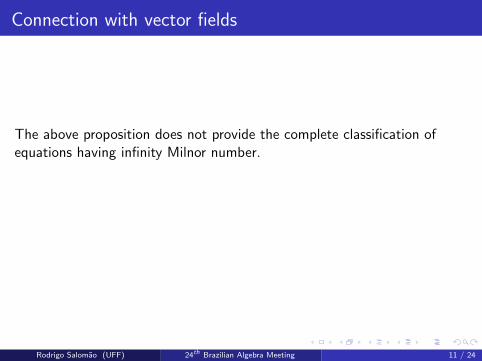
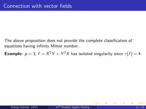
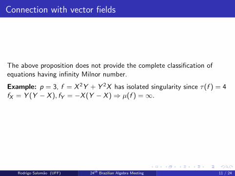
The above proposition does not provide the complete classification ofequations having infinity Milnor number.
Example: p = 3, f = X 2Y + Y 2X has isolated singularity since τ(f ) = 4fX = Y (Y − X ), fY = −X (Y − X )⇒ µ(f ) =∞.h = gcd(fX , fY ) = Y − X and fX/h = Y , fY /h = −X ∈ m.
Rodrigo Salomao (UFF) 24th Brazilian Algebra Meeting 11 / 24
Connection with vector fields
The above proposition does not provide the complete classification ofequations having infinity Milnor number.
Example: p = 3, f = X 2Y + Y 2X has isolated singularity since τ(f ) = 4
fX = Y (Y − X ), fY = −X (Y − X )⇒ µ(f ) =∞.h = gcd(fX , fY ) = Y − X and fX/h = Y , fY /h = −X ∈ m.
Rodrigo Salomao (UFF) 24th Brazilian Algebra Meeting 11 / 24
Connection with vector fields
The above proposition does not provide the complete classification ofequations having infinity Milnor number.
Example: p = 3, f = X 2Y + Y 2X has isolated singularity since τ(f ) = 4fX = Y (Y − X ), fY = −X (Y − X )⇒ µ(f ) =∞.
h = gcd(fX , fY ) = Y − X and fX/h = Y , fY /h = −X ∈ m.
Rodrigo Salomao (UFF) 24th Brazilian Algebra Meeting 11 / 24
Connection with vector fields
The above proposition does not provide the complete classification ofequations having infinity Milnor number.
Example: p = 3, f = X 2Y + Y 2X has isolated singularity since τ(f ) = 4fX = Y (Y − X ), fY = −X (Y − X )⇒ µ(f ) =∞.h = gcd(fX , fY ) = Y − X and fX/h = Y , fY /h = −X ∈ m.
Rodrigo Salomao (UFF) 24th Brazilian Algebra Meeting 11 / 24
Good equations and the invariant µ(O)
Let us consider I an ideal of R and g ∈ R.
We say that g is integral overI if there are ` ≥ 1 and a1, . . . , a` ∈ R with ai ∈ I i , satisfying
g ` + a1g`−1 + · · ·+ a` = 0.
The integral closure I of I is the set of all integral elements of R over I .
Let J ⊆ I be ideals of R. The ideal J is called a reduction of I if for somes ≥ 0 one has JI s = I s+1. In this case,
√J =√I .
J is called a minimal reduction of I if it is a reduction and it is minimalwith respect to the inclusion.
We denote by e0(I ) the Hilbert-Samuel multiplicity of an m-primary ideal Iof R and we put e0(I ) =∞ if I is not m-primary.
Rodrigo Salomao (UFF) 24th Brazilian Algebra Meeting 12 / 24
Good equations and the invariant µ(O)
Let us consider I an ideal of R and g ∈ R. We say that g is integral overI if there are ` ≥ 1 and a1, . . . , a` ∈ R with ai ∈ I i , satisfying
g ` + a1g`−1 + · · ·+ a` = 0.
The integral closure I of I is the set of all integral elements of R over I .
Let J ⊆ I be ideals of R.
The ideal J is called a reduction of I if for somes ≥ 0 one has JI s = I s+1. In this case,
√J =√I .
J is called a minimal reduction of I if it is a reduction and it is minimalwith respect to the inclusion.
We denote by e0(I ) the Hilbert-Samuel multiplicity of an m-primary ideal Iof R and we put e0(I ) =∞ if I is not m-primary.
Rodrigo Salomao (UFF) 24th Brazilian Algebra Meeting 12 / 24
Good equations and the invariant µ(O)
Let us consider I an ideal of R and g ∈ R. We say that g is integral overI if there are ` ≥ 1 and a1, . . . , a` ∈ R with ai ∈ I i , satisfying
g ` + a1g`−1 + · · ·+ a` = 0.
The integral closure I of I is the set of all integral elements of R over I .
Let J ⊆ I be ideals of R. The ideal J is called a reduction of I if for somes ≥ 0 one has JI s = I s+1.
In this case,√J =√I .
J is called a minimal reduction of I if it is a reduction and it is minimalwith respect to the inclusion.
We denote by e0(I ) the Hilbert-Samuel multiplicity of an m-primary ideal Iof R and we put e0(I ) =∞ if I is not m-primary.
Rodrigo Salomao (UFF) 24th Brazilian Algebra Meeting 12 / 24
Good equations and the invariant µ(O)
Let us consider I an ideal of R and g ∈ R. We say that g is integral overI if there are ` ≥ 1 and a1, . . . , a` ∈ R with ai ∈ I i , satisfying
g ` + a1g`−1 + · · ·+ a` = 0.
The integral closure I of I is the set of all integral elements of R over I .
Let J ⊆ I be ideals of R. The ideal J is called a reduction of I if for somes ≥ 0 one has JI s = I s+1. In this case,
√J =√I .
J is called a minimal reduction of I if it is a reduction and it is minimalwith respect to the inclusion.
We denote by e0(I ) the Hilbert-Samuel multiplicity of an m-primary ideal Iof R and we put e0(I ) =∞ if I is not m-primary.
Rodrigo Salomao (UFF) 24th Brazilian Algebra Meeting 12 / 24
Good equations and the invariant µ(O)
Let us consider I an ideal of R and g ∈ R. We say that g is integral overI if there are ` ≥ 1 and a1, . . . , a` ∈ R with ai ∈ I i , satisfying
g ` + a1g`−1 + · · ·+ a` = 0.
The integral closure I of I is the set of all integral elements of R over I .
Let J ⊆ I be ideals of R. The ideal J is called a reduction of I if for somes ≥ 0 one has JI s = I s+1. In this case,
√J =√I .
J is called a minimal reduction of I if it is a reduction and it is minimalwith respect to the inclusion.
We denote by e0(I ) the Hilbert-Samuel multiplicity of an m-primary ideal Iof R and we put e0(I ) =∞ if I is not m-primary.
Rodrigo Salomao (UFF) 24th Brazilian Algebra Meeting 12 / 24
Good equations and the invariant µ(O)
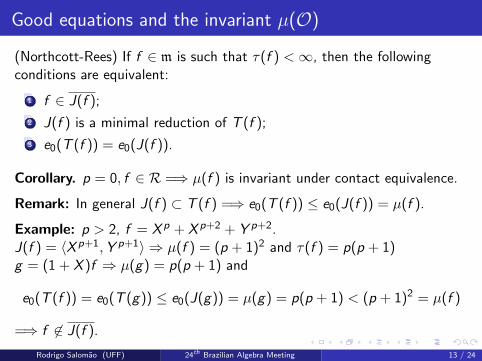
(Northcott-Rees) If f ∈ m is such that τ(f ) <∞, then the followingconditions are equivalent:
1 f ∈ J(f );
2 J(f ) is a minimal reduction of T (f );
3 e0(T (f )) = e0(J(f )).
Corollary. p = 0, f ∈ R =⇒ µ(f ) is invariant under contact equivalence.
Remark: In general J(f ) ⊂ T (f ) =⇒ e0(T (f )) ≤ e0(J(f )) = µ(f ).
Example: p > 2, f = X p + X p+2 + Y p+2.J(f ) = 〈X p+1,Y p+1〉 ⇒ µ(f ) = (p + 1)2 and τ(f ) = p(p + 1)g = (1 + X )f ⇒ µ(g) = p(p + 1) and
e0(T (f )) = e0(T (g)) ≤ e0(J(g)) = µ(g) = p(p + 1) < (p + 1)2 = µ(f )
=⇒ f 6∈ J(f ).
Rodrigo Salomao (UFF) 24th Brazilian Algebra Meeting 13 / 24
Good equations and the invariant µ(O)
(Northcott-Rees) If f ∈ m is such that τ(f ) <∞, then the followingconditions are equivalent:
1 f ∈ J(f );
2 J(f ) is a minimal reduction of T (f );
3 e0(T (f )) = e0(J(f )).
Corollary. p = 0, f ∈ R =⇒ µ(f ) is invariant under contact equivalence.
Remark: In general J(f ) ⊂ T (f ) =⇒ e0(T (f )) ≤ e0(J(f )) = µ(f ).
Example: p > 2, f = X p + X p+2 + Y p+2.J(f ) = 〈X p+1,Y p+1〉 ⇒ µ(f ) = (p + 1)2 and τ(f ) = p(p + 1)g = (1 + X )f ⇒ µ(g) = p(p + 1) and
e0(T (f )) = e0(T (g)) ≤ e0(J(g)) = µ(g) = p(p + 1) < (p + 1)2 = µ(f )
=⇒ f 6∈ J(f ).
Rodrigo Salomao (UFF) 24th Brazilian Algebra Meeting 13 / 24
Good equations and the invariant µ(O)
(Northcott-Rees) If f ∈ m is such that τ(f ) <∞, then the followingconditions are equivalent:
1 f ∈ J(f );
2 J(f ) is a minimal reduction of T (f );
3 e0(T (f )) = e0(J(f )).
Corollary. p = 0, f ∈ R =⇒ µ(f ) is invariant under contact equivalence.
Remark: In general J(f ) ⊂ T (f ) =⇒ e0(T (f )) ≤ e0(J(f )) = µ(f ).
Example: p > 2, f = X p + X p+2 + Y p+2.
J(f ) = 〈X p+1,Y p+1〉 ⇒ µ(f ) = (p + 1)2 and τ(f ) = p(p + 1)g = (1 + X )f ⇒ µ(g) = p(p + 1) and
e0(T (f )) = e0(T (g)) ≤ e0(J(g)) = µ(g) = p(p + 1) < (p + 1)2 = µ(f )
=⇒ f 6∈ J(f ).
Rodrigo Salomao (UFF) 24th Brazilian Algebra Meeting 13 / 24
Good equations and the invariant µ(O)
(Northcott-Rees) If f ∈ m is such that τ(f ) <∞, then the followingconditions are equivalent:
1 f ∈ J(f );
2 J(f ) is a minimal reduction of T (f );
3 e0(T (f )) = e0(J(f )).
Corollary. p = 0, f ∈ R =⇒ µ(f ) is invariant under contact equivalence.
Remark: In general J(f ) ⊂ T (f ) =⇒ e0(T (f )) ≤ e0(J(f )) = µ(f ).
Example: p > 2, f = X p + X p+2 + Y p+2.J(f ) = 〈X p+1,Y p+1〉 ⇒ µ(f ) = (p + 1)2 and τ(f ) = p(p + 1)
g = (1 + X )f ⇒ µ(g) = p(p + 1) and
e0(T (f )) = e0(T (g)) ≤ e0(J(g)) = µ(g) = p(p + 1) < (p + 1)2 = µ(f )
=⇒ f 6∈ J(f ).
Rodrigo Salomao (UFF) 24th Brazilian Algebra Meeting 13 / 24
Good equations and the invariant µ(O)
(Northcott-Rees) If f ∈ m is such that τ(f ) <∞, then the followingconditions are equivalent:
1 f ∈ J(f );
2 J(f ) is a minimal reduction of T (f );
3 e0(T (f )) = e0(J(f )).
Corollary. p = 0, f ∈ R =⇒ µ(f ) is invariant under contact equivalence.
Remark: In general J(f ) ⊂ T (f ) =⇒ e0(T (f )) ≤ e0(J(f )) = µ(f ).
Example: p > 2, f = X p + X p+2 + Y p+2.J(f ) = 〈X p+1,Y p+1〉 ⇒ µ(f ) = (p + 1)2 and τ(f ) = p(p + 1)g = (1 + X )f ⇒ µ(g) = p(p + 1) and
e0(T (f )) = e0(T (g)) ≤ e0(J(g)) = µ(g) = p(p + 1) < (p + 1)2 = µ(f )
=⇒ f 6∈ J(f ).
Rodrigo Salomao (UFF) 24th Brazilian Algebra Meeting 13 / 24
Good equations and the invariant µ(O)
(Northcott-Rees) If f ∈ m is such that τ(f ) <∞, then the followingconditions are equivalent:
1 f ∈ J(f );
2 J(f ) is a minimal reduction of T (f );
3 e0(T (f )) = e0(J(f )).
Corollary. p = 0, f ∈ R =⇒ µ(f ) is invariant under contact equivalence.
Remark: In general J(f ) ⊂ T (f ) =⇒ e0(T (f )) ≤ e0(J(f )) = µ(f ).
Example: p > 2, f = X p + X p+2 + Y p+2.J(f ) = 〈X p+1,Y p+1〉 ⇒ µ(f ) = (p + 1)2 and τ(f ) = p(p + 1)g = (1 + X )f ⇒ µ(g) = p(p + 1) and
e0(T (f )) = e0(T (g)) ≤ e0(J(g)) = µ(g) = p(p + 1) < (p + 1)2 = µ(f )
=⇒ f 6∈ J(f ).
Rodrigo Salomao (UFF) 24th Brazilian Algebra Meeting 13 / 24
Good equations and the invariant µ(O)
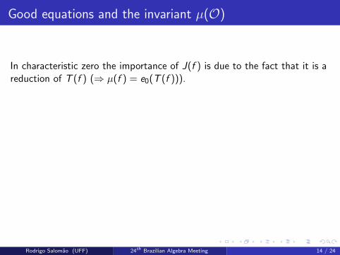
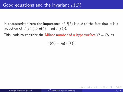
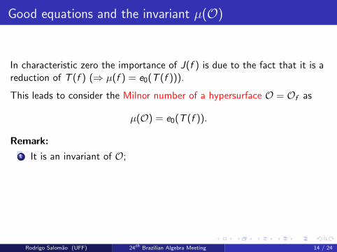
In characteristic zero the importance of J(f ) is due to the fact that it is areduction of T (f ) (⇒ µ(f ) = e0(T (f ))).
This leads to consider the Milnor number of a hypersurface O = Of as
µ(O) = e0(T (f )).
Remark:
1 It is an invariant of O;
2 p = 0⇒ µ(O) = µ(f ) for any equation f of O;
We call an equation f of O a good equation if f ∈ J(f ).
Rodrigo Salomao (UFF) 24th Brazilian Algebra Meeting 14 / 24
Good equations and the invariant µ(O)
In characteristic zero the importance of J(f ) is due to the fact that it is areduction of T (f ) (⇒ µ(f ) = e0(T (f ))).
This leads to consider the Milnor number of a hypersurface O = Of as
µ(O) = e0(T (f )).
Remark:
1 It is an invariant of O;
2 p = 0⇒ µ(O) = µ(f ) for any equation f of O;
We call an equation f of O a good equation if f ∈ J(f ).
Rodrigo Salomao (UFF) 24th Brazilian Algebra Meeting 14 / 24
Variation of µ(uf ) and computation of µ(O)
Last example shows that there are bad equations since we have theexistence of f ∈ R such that e0(T (f )) < µ(f ).
Good news: good equations are “generic” in the contact class.
Rodrigo Salomao (UFF) 24th Brazilian Algebra Meeting 15 / 24
Variation of µ(uf ) and computation of µ(O)
Last example shows that there are bad equations since we have theexistence of f ∈ R such that e0(T (f )) < µ(f ).
Good news: good equations are “generic” in the contact class.
Rodrigo Salomao (UFF) 24th Brazilian Algebra Meeting 15 / 24
Variation of µ(uf ) and computation of µ(O)
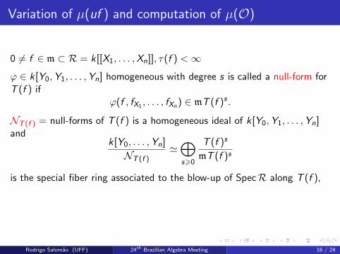
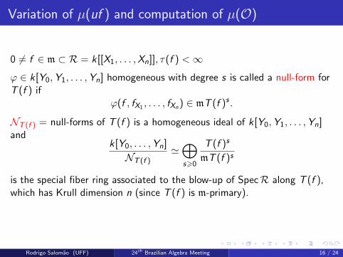
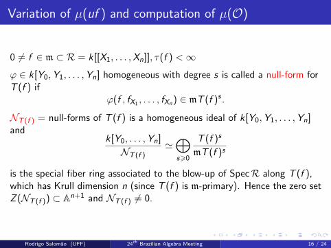
0 6= f ∈ m ⊂ R = k[[X1, . . . ,Xn]], τ(f ) <∞
ϕ ∈ k[Y0,Y1, . . . ,Yn] homogeneous with degree s is called a null-form forT (f ) if
ϕ(f , fX1 , . . . , fXn) ∈ mT (f )s .
NT (f ) = null-forms of T (f ) is a homogeneous ideal of k[Y0,Y1, . . . ,Yn]and
k[Y0, . . . ,Yn]
NT (f )'⊕s>0
T (f )s
mT (f )s
is the special fiber ring associated to the blow-up of SpecR along T (f ),which has Krull dimension n (since T (f ) is m-primary). Hence the zero setZ (NT (f )) ⊂ An+1 and NT (f ) 6= 0.
Rodrigo Salomao (UFF) 24th Brazilian Algebra Meeting 16 / 24
Variation of µ(uf ) and computation of µ(O)
0 6= f ∈ m ⊂ R = k[[X1, . . . ,Xn]], τ(f ) <∞
ϕ ∈ k[Y0,Y1, . . . ,Yn] homogeneous with degree s
is called a null-form forT (f ) if
ϕ(f , fX1 , . . . , fXn) ∈ mT (f )s .
NT (f ) = null-forms of T (f ) is a homogeneous ideal of k[Y0,Y1, . . . ,Yn]and
k[Y0, . . . ,Yn]
NT (f )'⊕s>0
T (f )s
mT (f )s
is the special fiber ring associated to the blow-up of SpecR along T (f ),which has Krull dimension n (since T (f ) is m-primary). Hence the zero setZ (NT (f )) ⊂ An+1 and NT (f ) 6= 0.
Rodrigo Salomao (UFF) 24th Brazilian Algebra Meeting 16 / 24
Variation of µ(uf ) and computation of µ(O)
0 6= f ∈ m ⊂ R = k[[X1, . . . ,Xn]], τ(f ) <∞
ϕ ∈ k[Y0,Y1, . . . ,Yn] homogeneous with degree s is called a null-form forT (f ) if
ϕ(f , fX1 , . . . , fXn) ∈ mT (f )s .
NT (f ) = null-forms of T (f ) is a homogeneous ideal of k[Y0,Y1, . . . ,Yn]and
k[Y0, . . . ,Yn]
NT (f )'⊕s>0
T (f )s
mT (f )s
is the special fiber ring associated to the blow-up of SpecR along T (f ),which has Krull dimension n (since T (f ) is m-primary). Hence the zero setZ (NT (f )) ⊂ An+1 and NT (f ) 6= 0.
Rodrigo Salomao (UFF) 24th Brazilian Algebra Meeting 16 / 24
Variation of µ(uf ) and computation of µ(O)
0 6= f ∈ m ⊂ R = k[[X1, . . . ,Xn]], τ(f ) <∞
ϕ ∈ k[Y0,Y1, . . . ,Yn] homogeneous with degree s is called a null-form forT (f ) if
ϕ(f , fX1 , . . . , fXn) ∈ mT (f )s .
NT (f ) = null-forms of T (f ) is a homogeneous ideal of k[Y0,Y1, . . . ,Yn]
andk[Y0, . . . ,Yn]
NT (f )'⊕s>0
T (f )s
mT (f )s
is the special fiber ring associated to the blow-up of SpecR along T (f ),which has Krull dimension n (since T (f ) is m-primary). Hence the zero setZ (NT (f )) ⊂ An+1 and NT (f ) 6= 0.
Rodrigo Salomao (UFF) 24th Brazilian Algebra Meeting 16 / 24
Variation of µ(uf ) and computation of µ(O)
0 6= f ∈ m ⊂ R = k[[X1, . . . ,Xn]], τ(f ) <∞
ϕ ∈ k[Y0,Y1, . . . ,Yn] homogeneous with degree s is called a null-form forT (f ) if
ϕ(f , fX1 , . . . , fXn) ∈ mT (f )s .
NT (f ) = null-forms of T (f ) is a homogeneous ideal of k[Y0,Y1, . . . ,Yn]and
k[Y0, . . . ,Yn]
NT (f )'⊕s>0
T (f )s
mT (f )s
is the special fiber ring associated to the blow-up of SpecR along T (f ),
which has Krull dimension n (since T (f ) is m-primary). Hence the zero setZ (NT (f )) ⊂ An+1 and NT (f ) 6= 0.
Rodrigo Salomao (UFF) 24th Brazilian Algebra Meeting 16 / 24
Variation of µ(uf ) and computation of µ(O)
0 6= f ∈ m ⊂ R = k[[X1, . . . ,Xn]], τ(f ) <∞
ϕ ∈ k[Y0,Y1, . . . ,Yn] homogeneous with degree s is called a null-form forT (f ) if
ϕ(f , fX1 , . . . , fXn) ∈ mT (f )s .
NT (f ) = null-forms of T (f ) is a homogeneous ideal of k[Y0,Y1, . . . ,Yn]and
k[Y0, . . . ,Yn]
NT (f )'⊕s>0
T (f )s
mT (f )s
is the special fiber ring associated to the blow-up of SpecR along T (f ),which has Krull dimension n (since T (f ) is m-primary).
Hence the zero setZ (NT (f )) ⊂ An+1 and NT (f ) 6= 0.
Rodrigo Salomao (UFF) 24th Brazilian Algebra Meeting 16 / 24
Variation of µ(uf ) and computation of µ(O)
0 6= f ∈ m ⊂ R = k[[X1, . . . ,Xn]], τ(f ) <∞
ϕ ∈ k[Y0,Y1, . . . ,Yn] homogeneous with degree s is called a null-form forT (f ) if
ϕ(f , fX1 , . . . , fXn) ∈ mT (f )s .
NT (f ) = null-forms of T (f ) is a homogeneous ideal of k[Y0,Y1, . . . ,Yn]and
k[Y0, . . . ,Yn]
NT (f )'⊕s>0
T (f )s
mT (f )s
is the special fiber ring associated to the blow-up of SpecR along T (f ),which has Krull dimension n (since T (f ) is m-primary). Hence the zero setZ (NT (f )) ⊂ An+1 and NT (f ) 6= 0.
Rodrigo Salomao (UFF) 24th Brazilian Algebra Meeting 16 / 24
Variation of µ(uf ) and computation of µ(O)
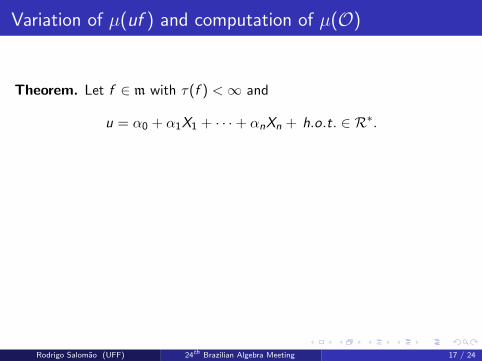
Theorem. Let f ∈ m with τ(f ) <∞ and
u = α0 + α1X1 + · · ·+ αnXn + h.o.t. ∈ R∗.
We have that uf ∈ J(uf ) if and only if there exists G ∈ NT (f ) such thatG (α0,−α1, . . . ,−αn) 6= 0.
Consequences:
uf ∈ J(uf ) hold for u ∈ R∗ generic;
for a generic u ∈ R∗ we have µ(Of ) = µ(uf ).
µ(Of ) = min{µ(uf ), u ∈ R∗}.
Rodrigo Salomao (UFF) 24th Brazilian Algebra Meeting 17 / 24
Variation of µ(uf ) and computation of µ(O)
Theorem. f ∈ m with τ(f ) <∞. The following conditions are equivalent.
1 µ(uf ) = µ(Of ) for all u ∈ R∗;2 Z (NT (f )) = Z (Y0);
3 f ` ∈ mT (f )`, for some ` ≥ 1.
In this case we say that f is µ-stable
Example: f ∈ k[X1, . . . ,Xn] quasi-homogeneous of degree d with p - d .
There are integers d1, . . . , dn such that df = d1X1fX1 + · · ·+ dnXnfXn .Hence f ∈ mT (f ) and is µ-stable.
Rodrigo Salomao (UFF) 24th Brazilian Algebra Meeting 18 / 24
Variation of µ(uf ) and computation of µ(O)
Theorem. f ∈ m with τ(f ) <∞. The following conditions are equivalent.
1 µ(uf ) = µ(Of ) for all u ∈ R∗;
2 Z (NT (f )) = Z (Y0);
3 f ` ∈ mT (f )`, for some ` ≥ 1.
In this case we say that f is µ-stable
Example: f ∈ k[X1, . . . ,Xn] quasi-homogeneous of degree d with p - d .
There are integers d1, . . . , dn such that df = d1X1fX1 + · · ·+ dnXnfXn .Hence f ∈ mT (f ) and is µ-stable.
Rodrigo Salomao (UFF) 24th Brazilian Algebra Meeting 18 / 24
Variation of µ(uf ) and computation of µ(O)
Theorem. f ∈ m with τ(f ) <∞. The following conditions are equivalent.
1 µ(uf ) = µ(Of ) for all u ∈ R∗;2 Z (NT (f )) = Z (Y0);
3 f ` ∈ mT (f )`, for some ` ≥ 1.
In this case we say that f is µ-stable
Example: f ∈ k[X1, . . . ,Xn] quasi-homogeneous of degree d with p - d .
There are integers d1, . . . , dn such that df = d1X1fX1 + · · ·+ dnXnfXn .Hence f ∈ mT (f ) and is µ-stable.
Rodrigo Salomao (UFF) 24th Brazilian Algebra Meeting 18 / 24
Variation of µ(uf ) and computation of µ(O)
Theorem. f ∈ m with τ(f ) <∞. The following conditions are equivalent.
1 µ(uf ) = µ(Of ) for all u ∈ R∗;2 Z (NT (f )) = Z (Y0);
3 f ` ∈ mT (f )`, for some ` ≥ 1.
In this case we say that f is µ-stable
Example: f ∈ k[X1, . . . ,Xn] quasi-homogeneous of degree d with p - d .
There are integers d1, . . . , dn such that df = d1X1fX1 + · · ·+ dnXnfXn .
Hence f ∈ mT (f ) and is µ-stable.
Rodrigo Salomao (UFF) 24th Brazilian Algebra Meeting 18 / 24
Variation of µ(uf ) and computation of µ(O)
Theorem. f ∈ m with τ(f ) <∞. The following conditions are equivalent.
1 µ(uf ) = µ(Of ) for all u ∈ R∗;2 Z (NT (f )) = Z (Y0);
3 f ` ∈ mT (f )`, for some ` ≥ 1.
In this case we say that f is µ-stable
Example: f ∈ k[X1, . . . ,Xn] quasi-homogeneous of degree d with p - d .
There are integers d1, . . . , dn such that df = d1X1fX1 + · · ·+ dnXnfXn .Hence f ∈ mT (f ) and is µ-stable.
Rodrigo Salomao (UFF) 24th Brazilian Algebra Meeting 18 / 24
Plane Branches
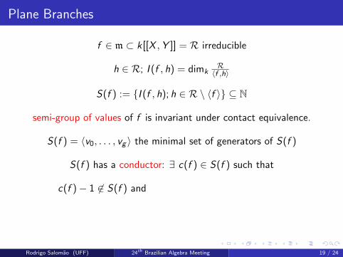
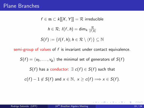
f ∈ m ⊂ k[[X ,Y ]] = R irreducible
h ∈ R; I (f , h) = dimkR〈f ,h〉
S(f ) := {I (f , h); h ∈ R \ 〈f 〉} ⊆ N
semi-group of values of f is invariant under contact equivalence.
S(f ) = 〈v0, . . . , vg 〉 the minimal set of generators of S(f )
S(f ) has a conductor: ∃ c(f ) ∈ S(f ) such that
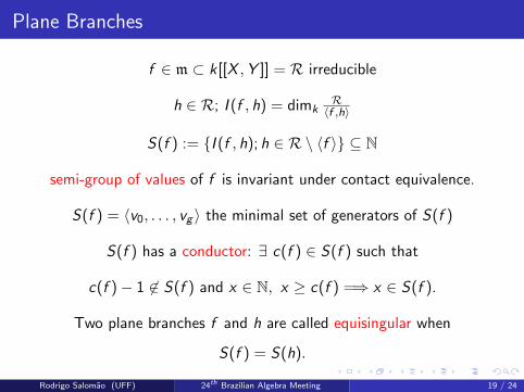
c(f )− 1 6∈ S(f ) and x ∈ N, x ≥ c(f ) =⇒ x ∈ S(f ).
Two plane branches f and h are called equisingular when
S(f ) = S(h).
Rodrigo Salomao (UFF) 24th Brazilian Algebra Meeting 19 / 24
Plane Branches
f ∈ m ⊂ k[[X ,Y ]] = R irreducible
h ∈ R;
I (f , h) = dimkR〈f ,h〉
S(f ) := {I (f , h); h ∈ R \ 〈f 〉} ⊆ N
semi-group of values of f is invariant under contact equivalence.
S(f ) = 〈v0, . . . , vg 〉 the minimal set of generators of S(f )
S(f ) has a conductor: ∃ c(f ) ∈ S(f ) such that
c(f )− 1 6∈ S(f ) and x ∈ N, x ≥ c(f ) =⇒ x ∈ S(f ).
Two plane branches f and h are called equisingular when
S(f ) = S(h).
Rodrigo Salomao (UFF) 24th Brazilian Algebra Meeting 19 / 24
Plane Branches
f ∈ m ⊂ k[[X ,Y ]] = R irreducible
h ∈ R; I (f , h) = dimkR〈f ,h〉
S(f ) := {I (f , h); h ∈ R \ 〈f 〉} ⊆ N
semi-group of values of f is invariant under contact equivalence.
S(f ) = 〈v0, . . . , vg 〉 the minimal set of generators of S(f )
S(f ) has a conductor: ∃ c(f ) ∈ S(f ) such that
c(f )− 1 6∈ S(f ) and x ∈ N, x ≥ c(f ) =⇒ x ∈ S(f ).
Two plane branches f and h are called equisingular when
S(f ) = S(h).
Rodrigo Salomao (UFF) 24th Brazilian Algebra Meeting 19 / 24
Plane Branches
f ∈ m ⊂ k[[X ,Y ]] = R irreducible
h ∈ R; I (f , h) = dimkR〈f ,h〉
S(f ) := {I (f , h); h ∈ R \ 〈f 〉} ⊆ N
semi-group of values of f
is invariant under contact equivalence.
S(f ) = 〈v0, . . . , vg 〉 the minimal set of generators of S(f )
S(f ) has a conductor: ∃ c(f ) ∈ S(f ) such that
c(f )− 1 6∈ S(f ) and x ∈ N, x ≥ c(f ) =⇒ x ∈ S(f ).
Two plane branches f and h are called equisingular when
S(f ) = S(h).
Rodrigo Salomao (UFF) 24th Brazilian Algebra Meeting 19 / 24
Plane Branches
f ∈ m ⊂ k[[X ,Y ]] = R irreducible
h ∈ R; I (f , h) = dimkR〈f ,h〉
S(f ) := {I (f , h); h ∈ R \ 〈f 〉} ⊆ N
semi-group of values of f is invariant under contact equivalence.
S(f ) = 〈v0, . . . , vg 〉 the minimal set of generators of S(f )
S(f ) has a conductor: ∃ c(f ) ∈ S(f ) such that
c(f )− 1 6∈ S(f ) and x ∈ N, x ≥ c(f ) =⇒ x ∈ S(f ).
Two plane branches f and h are called equisingular when
S(f ) = S(h).
Rodrigo Salomao (UFF) 24th Brazilian Algebra Meeting 19 / 24
Plane Branches
f ∈ m ⊂ k[[X ,Y ]] = R irreducible
h ∈ R; I (f , h) = dimkR〈f ,h〉
S(f ) := {I (f , h); h ∈ R \ 〈f 〉} ⊆ N
semi-group of values of f is invariant under contact equivalence.
S(f ) = 〈v0, . . . , vg 〉 the minimal set of generators of S(f )
S(f ) has a conductor:
∃ c(f ) ∈ S(f ) such that
c(f )− 1 6∈ S(f ) and x ∈ N, x ≥ c(f ) =⇒ x ∈ S(f ).
Two plane branches f and h are called equisingular when
S(f ) = S(h).
Rodrigo Salomao (UFF) 24th Brazilian Algebra Meeting 19 / 24
Plane Branches
f ∈ m ⊂ k[[X ,Y ]] = R irreducible
h ∈ R; I (f , h) = dimkR〈f ,h〉
S(f ) := {I (f , h); h ∈ R \ 〈f 〉} ⊆ N
semi-group of values of f is invariant under contact equivalence.
S(f ) = 〈v0, . . . , vg 〉 the minimal set of generators of S(f )
S(f ) has a conductor: ∃ c(f ) ∈ S(f ) such that
c(f )− 1 6∈ S(f ) and x ∈ N, x ≥ c(f ) =⇒ x ∈ S(f ).
Two plane branches f and h are called equisingular when
S(f ) = S(h).
Rodrigo Salomao (UFF) 24th Brazilian Algebra Meeting 19 / 24
Plane Branches
f ∈ m ⊂ k[[X ,Y ]] = R irreducible
h ∈ R; I (f , h) = dimkR〈f ,h〉
S(f ) := {I (f , h); h ∈ R \ 〈f 〉} ⊆ N
semi-group of values of f is invariant under contact equivalence.
S(f ) = 〈v0, . . . , vg 〉 the minimal set of generators of S(f )
S(f ) has a conductor: ∃ c(f ) ∈ S(f ) such that
c(f )− 1 6∈ S(f ) and
x ∈ N, x ≥ c(f ) =⇒ x ∈ S(f ).
Two plane branches f and h are called equisingular when
S(f ) = S(h).
Rodrigo Salomao (UFF) 24th Brazilian Algebra Meeting 19 / 24
Plane Branches
f ∈ m ⊂ k[[X ,Y ]] = R irreducible
h ∈ R; I (f , h) = dimkR〈f ,h〉
S(f ) := {I (f , h); h ∈ R \ 〈f 〉} ⊆ N
semi-group of values of f is invariant under contact equivalence.
S(f ) = 〈v0, . . . , vg 〉 the minimal set of generators of S(f )
S(f ) has a conductor: ∃ c(f ) ∈ S(f ) such that
c(f )− 1 6∈ S(f ) and x ∈ N, x ≥ c(f ) =⇒ x ∈ S(f ).
Two plane branches f and h are called equisingular when
S(f ) = S(h).
Rodrigo Salomao (UFF) 24th Brazilian Algebra Meeting 19 / 24
Plane Branches
f ∈ m ⊂ k[[X ,Y ]] = R irreducible
h ∈ R; I (f , h) = dimkR〈f ,h〉
S(f ) := {I (f , h); h ∈ R \ 〈f 〉} ⊆ N
semi-group of values of f is invariant under contact equivalence.
S(f ) = 〈v0, . . . , vg 〉 the minimal set of generators of S(f )
S(f ) has a conductor: ∃ c(f ) ∈ S(f ) such that
c(f )− 1 6∈ S(f ) and x ∈ N, x ≥ c(f ) =⇒ x ∈ S(f ).
Two plane branches f and h are called equisingular when
S(f ) = S(h).
Rodrigo Salomao (UFF) 24th Brazilian Algebra Meeting 19 / 24
Plane Branches
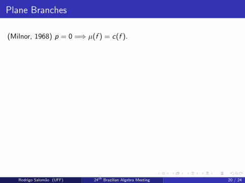
(Milnor, 1968) p = 0 =⇒ µ(f ) = c(f ).
In particular, µ is an invariant of the equisingularity class. It may fails ifp > 0.
Example: f = (Y 2 − X 3)2 − X 11Y and h = (Y 2 − X 3 + X 2Y )2 − X 11Yare equisingular with S(f ) = S(h) = 〈4, 6, 25〉 and c(f ) = c(h) = 28. Ifp = 5 we have µ(f ) = 41 6= 30 = µ(Of ) ⇒ f is not µ-stableh3 ∈ mT (h)3⇒ h is µ-stable: µ(Oh) = µ(h) = 29.
µ-stability is not preserved in the same equisingularity class;
Neither the Milnor number of a hypersurface is.
Note that p divides one of the generators of S(f ).
Rodrigo Salomao (UFF) 24th Brazilian Algebra Meeting 20 / 24
Plane Branches
(Milnor, 1968) p = 0 =⇒ µ(f ) = c(f ).
In particular, µ is an invariant of the equisingularity class.
It may fails ifp > 0.
Example: f = (Y 2 − X 3)2 − X 11Y and h = (Y 2 − X 3 + X 2Y )2 − X 11Yare equisingular with S(f ) = S(h) = 〈4, 6, 25〉 and c(f ) = c(h) = 28. Ifp = 5 we have µ(f ) = 41 6= 30 = µ(Of ) ⇒ f is not µ-stableh3 ∈ mT (h)3⇒ h is µ-stable: µ(Oh) = µ(h) = 29.
µ-stability is not preserved in the same equisingularity class;
Neither the Milnor number of a hypersurface is.
Note that p divides one of the generators of S(f ).
Rodrigo Salomao (UFF) 24th Brazilian Algebra Meeting 20 / 24
Plane Branches
(Milnor, 1968) p = 0 =⇒ µ(f ) = c(f ).
In particular, µ is an invariant of the equisingularity class. It may fails ifp > 0.
Example: f = (Y 2 − X 3)2 − X 11Y and h = (Y 2 − X 3 + X 2Y )2 − X 11Yare equisingular with S(f ) = S(h) = 〈4, 6, 25〉 and c(f ) = c(h) = 28. Ifp = 5 we have µ(f ) = 41 6= 30 = µ(Of ) ⇒ f is not µ-stableh3 ∈ mT (h)3⇒ h is µ-stable: µ(Oh) = µ(h) = 29.
µ-stability is not preserved in the same equisingularity class;
Neither the Milnor number of a hypersurface is.
Note that p divides one of the generators of S(f ).
Rodrigo Salomao (UFF) 24th Brazilian Algebra Meeting 20 / 24
Plane Branches
(Milnor, 1968) p = 0 =⇒ µ(f ) = c(f ).
In particular, µ is an invariant of the equisingularity class. It may fails ifp > 0.
Example: f = (Y 2 − X 3)2 − X 11Y and h = (Y 2 − X 3 + X 2Y )2 − X 11Yare equisingular with S(f ) = S(h) = 〈4, 6, 25〉 and c(f ) = c(h) = 28.
Ifp = 5 we have µ(f ) = 41 6= 30 = µ(Of ) ⇒ f is not µ-stableh3 ∈ mT (h)3⇒ h is µ-stable: µ(Oh) = µ(h) = 29.
µ-stability is not preserved in the same equisingularity class;
Neither the Milnor number of a hypersurface is.
Note that p divides one of the generators of S(f ).
Rodrigo Salomao (UFF) 24th Brazilian Algebra Meeting 20 / 24
Plane Branches
(Milnor, 1968) p = 0 =⇒ µ(f ) = c(f ).
In particular, µ is an invariant of the equisingularity class. It may fails ifp > 0.
Example: f = (Y 2 − X 3)2 − X 11Y and h = (Y 2 − X 3 + X 2Y )2 − X 11Yare equisingular with S(f ) = S(h) = 〈4, 6, 25〉 and c(f ) = c(h) = 28. Ifp = 5 we have
µ(f ) = 41 6= 30 = µ(Of ) ⇒ f is not µ-stableh3 ∈ mT (h)3⇒ h is µ-stable: µ(Oh) = µ(h) = 29.
µ-stability is not preserved in the same equisingularity class;
Neither the Milnor number of a hypersurface is.
Note that p divides one of the generators of S(f ).
Rodrigo Salomao (UFF) 24th Brazilian Algebra Meeting 20 / 24
Plane Branches
(Milnor, 1968) p = 0 =⇒ µ(f ) = c(f ).
In particular, µ is an invariant of the equisingularity class. It may fails ifp > 0.
Example: f = (Y 2 − X 3)2 − X 11Y and h = (Y 2 − X 3 + X 2Y )2 − X 11Yare equisingular with S(f ) = S(h) = 〈4, 6, 25〉 and c(f ) = c(h) = 28. Ifp = 5 we have µ(f ) = 41 6= 30 = µ(Of )
⇒ f is not µ-stableh3 ∈ mT (h)3⇒ h is µ-stable: µ(Oh) = µ(h) = 29.
µ-stability is not preserved in the same equisingularity class;
Neither the Milnor number of a hypersurface is.
Note that p divides one of the generators of S(f ).
Rodrigo Salomao (UFF) 24th Brazilian Algebra Meeting 20 / 24
Plane Branches
(Milnor, 1968) p = 0 =⇒ µ(f ) = c(f ).
In particular, µ is an invariant of the equisingularity class. It may fails ifp > 0.
Example: f = (Y 2 − X 3)2 − X 11Y and h = (Y 2 − X 3 + X 2Y )2 − X 11Yare equisingular with S(f ) = S(h) = 〈4, 6, 25〉 and c(f ) = c(h) = 28. Ifp = 5 we have µ(f ) = 41 6= 30 = µ(Of ) ⇒ f is not µ-stable
h3 ∈ mT (h)3⇒ h is µ-stable: µ(Oh) = µ(h) = 29.
µ-stability is not preserved in the same equisingularity class;
Neither the Milnor number of a hypersurface is.
Note that p divides one of the generators of S(f ).
Rodrigo Salomao (UFF) 24th Brazilian Algebra Meeting 20 / 24
Plane Branches
(Milnor, 1968) p = 0 =⇒ µ(f ) = c(f ).
In particular, µ is an invariant of the equisingularity class. It may fails ifp > 0.
Example: f = (Y 2 − X 3)2 − X 11Y and h = (Y 2 − X 3 + X 2Y )2 − X 11Yare equisingular with S(f ) = S(h) = 〈4, 6, 25〉 and c(f ) = c(h) = 28. Ifp = 5 we have µ(f ) = 41 6= 30 = µ(Of ) ⇒ f is not µ-stableh3 ∈ mT (h)3
⇒ h is µ-stable: µ(Oh) = µ(h) = 29.
µ-stability is not preserved in the same equisingularity class;
Neither the Milnor number of a hypersurface is.
Note that p divides one of the generators of S(f ).
Rodrigo Salomao (UFF) 24th Brazilian Algebra Meeting 20 / 24
Plane Branches
(Milnor, 1968) p = 0 =⇒ µ(f ) = c(f ).
In particular, µ is an invariant of the equisingularity class. It may fails ifp > 0.
Example: f = (Y 2 − X 3)2 − X 11Y and h = (Y 2 − X 3 + X 2Y )2 − X 11Yare equisingular with S(f ) = S(h) = 〈4, 6, 25〉 and c(f ) = c(h) = 28. Ifp = 5 we have µ(f ) = 41 6= 30 = µ(Of ) ⇒ f is not µ-stableh3 ∈ mT (h)3⇒ h is µ-stable:
µ(Oh) = µ(h) = 29.
µ-stability is not preserved in the same equisingularity class;
Neither the Milnor number of a hypersurface is.
Note that p divides one of the generators of S(f ).
Rodrigo Salomao (UFF) 24th Brazilian Algebra Meeting 20 / 24
Plane Branches
(Milnor, 1968) p = 0 =⇒ µ(f ) = c(f ).
In particular, µ is an invariant of the equisingularity class. It may fails ifp > 0.
Example: f = (Y 2 − X 3)2 − X 11Y and h = (Y 2 − X 3 + X 2Y )2 − X 11Yare equisingular with S(f ) = S(h) = 〈4, 6, 25〉 and c(f ) = c(h) = 28. Ifp = 5 we have µ(f ) = 41 6= 30 = µ(Of ) ⇒ f is not µ-stableh3 ∈ mT (h)3⇒ h is µ-stable: µ(Oh) = µ(h) = 29.
µ-stability is not preserved in the same equisingularity class;
Neither the Milnor number of a hypersurface is.
Note that p divides one of the generators of S(f ).
Rodrigo Salomao (UFF) 24th Brazilian Algebra Meeting 20 / 24
Plane Branches
(Milnor, 1968) p = 0 =⇒ µ(f ) = c(f ).
In particular, µ is an invariant of the equisingularity class. It may fails ifp > 0.
Example: f = (Y 2 − X 3)2 − X 11Y and h = (Y 2 − X 3 + X 2Y )2 − X 11Yare equisingular with S(f ) = S(h) = 〈4, 6, 25〉 and c(f ) = c(h) = 28. Ifp = 5 we have µ(f ) = 41 6= 30 = µ(Of ) ⇒ f is not µ-stableh3 ∈ mT (h)3⇒ h is µ-stable: µ(Oh) = µ(h) = 29.
µ-stability is not preserved in the same equisingularity class;
Neither the Milnor number of a hypersurface is.
Note that p divides one of the generators of S(f ).
Rodrigo Salomao (UFF) 24th Brazilian Algebra Meeting 20 / 24
Plane Branches
We say that S(f ) = 〈v0, . . . , vg 〉 is tame if p - v0v1 · · · vg .
(Deligne, 1973): In general, µ(f ) ≥ c(f ). Also, the difference µ(f )− c(f )counts the number of wild vanishing cycles.
Theorem. If f ∈ m2 is a plane branch singularity with S(f ) tame, then
µ(f ) = µ(Of ) = c(f ).
In particular, Of is µ-stable.
Rodrigo Salomao (UFF) 24th Brazilian Algebra Meeting 21 / 24

Plane Branches
µ-stability does not imply that the semi-group is tame;
We have strong evidences to believe that
µ(f ) = c(f ) =⇒ S(f ) is tame.
(Garcıa-Barroso and Ploski, 2015) The equivalence holds if
p > v0 = mult(f ).
Rodrigo Salomao (UFF) 24th Brazilian Algebra Meeting 22 / 24
Plane Branches
µ-stability does not imply that the semi-group is tame;
We have strong evidences to believe that
µ(f ) = c(f ) =⇒ S(f ) is tame.
(Garcıa-Barroso and Ploski, 2015) The equivalence holds if
p > v0 = mult(f ).
Rodrigo Salomao (UFF) 24th Brazilian Algebra Meeting 22 / 24
Plane Branches
µ-stability does not imply that the semi-group is tame;
We have strong evidences to believe that
µ(f ) = c(f ) =⇒ S(f ) is tame.
(Garcıa-Barroso and Ploski, 2015) The equivalence holds if
p > v0 = mult(f ).
Rodrigo Salomao (UFF) 24th Brazilian Algebra Meeting 22 / 24
About a result of Zariski
(Zariski, 1966): If f is a plane branch and char k = 0, thenc(f ) = τ(f ) ⇐⇒ up to change coordinates f = Y n −Xm with n and mrelatively primes.
In particular S(f ) = 〈n,m〉.
Countre-Example if p > 0: Consider p = 7 andf = (Y 2 − X 3)2 − 4X 8Y − X 13. ThenS(f ) = 〈4, 6, 19〉 is tameµ(f ) = c(f ) = 22 = τ(f ).
Rodrigo Salomao (UFF) 24th Brazilian Algebra Meeting 23 / 24
About a result of Zariski
(Zariski, 1966): If f is a plane branch and char k = 0, thenc(f ) = τ(f ) ⇐⇒ up to change coordinates f = Y n −Xm with n and mrelatively primes.
In particular S(f ) = 〈n,m〉.
Countre-Example if p > 0: Consider p = 7 andf = (Y 2 − X 3)2 − 4X 8Y − X 13.
ThenS(f ) = 〈4, 6, 19〉 is tameµ(f ) = c(f ) = 22 = τ(f ).
Rodrigo Salomao (UFF) 24th Brazilian Algebra Meeting 23 / 24
About a result of Zariski
(Zariski, 1966): If f is a plane branch and char k = 0, thenc(f ) = τ(f ) ⇐⇒ up to change coordinates f = Y n −Xm with n and mrelatively primes.
In particular S(f ) = 〈n,m〉.
Countre-Example if p > 0: Consider p = 7 andf = (Y 2 − X 3)2 − 4X 8Y − X 13. ThenS(f ) = 〈4, 6, 19〉 is tame
µ(f ) = c(f ) = 22 = τ(f ).
Rodrigo Salomao (UFF) 24th Brazilian Algebra Meeting 23 / 24
About a result of Zariski
(Zariski, 1966): If f is a plane branch and char k = 0, thenc(f ) = τ(f ) ⇐⇒ up to change coordinates f = Y n −Xm with n and mrelatively primes.
In particular S(f ) = 〈n,m〉.
Countre-Example if p > 0: Consider p = 7 andf = (Y 2 − X 3)2 − 4X 8Y − X 13. ThenS(f ) = 〈4, 6, 19〉 is tameµ(f ) = c(f ) = 22 = τ(f ).
Rodrigo Salomao (UFF) 24th Brazilian Algebra Meeting 23 / 24

THANK YOU!
Rodrigo Salomao (UFF) 24th Brazilian Algebra Meeting 24 / 24