JOURNAL OF PURE AND

ELSEVIER Journal of Pure and Applied Algebra 117 & 118 (1997) 353-379

APPLIED ALGEBRA

An algorithm for computing invariants of differential Galois groups’

Mark van Hoeij a,*, Jacques-Arthur Weil b a Departmen of Mathemutics, Universily of Nijmeyen, 6525 ED Nijmegen, Netherlands

b Dhpartement Mathkmatiques, FacultC des Sciences, 123 Au. Albert Thomas, F-87060 Limoges. France

Abstract

This paper presents an algorithm to compute invariants of the differential Galois group of linear differential equations L(y) = 0: if V(L) is the vector space of solutions of L(y) = 0, we show how given some integer m, one can compute the elements of the symmetric power Sym”‘( V(L)) that are left fixed by the Galois group. The bottleneck of previous methods is the construction of a differential operator called the ‘symmetric power of L’. Our strategy is to split the work into first a fast heuristic that produces a space that contains all invariants, and second a criterion to select all candidates that are really invariants.

The heuristic is built by generalizing the notion of exponents. The checking criterion is ob- tained by converting candidate invariants to candidate dual first integrals; this conversion is done efficiently by using a symmetric power of a formal solution matrix and showing how one can reduce significantly the number of entries of this matrix that need to be evaluated. @ 1997 Published by Elsevier Science B.V.

1991 Math. Subj. Class.: 68440, 34A05, 13A50

1. Introduction

Let C be a field of characteristic 0 and c be its algebraic closure. Denote k = c(x)

with the derivation 8 = (d/dx). Let

L(y)= ~Uiy(')=O, an # 0, ai E ml i=O

* Corresponding author. E-mail: hoeij@sci.kun.nl. ’ The work in this paper was prepared in the Dutch NW0 project AIDA.

0022-4049/97/%17.00 @ 1997 Published by Elsevier Science B.V. All rights reserved Z’IZ SOO22-4049(97)000 18-2

354 M. van Hoe& J.-A. WeillJournal of Pure and Applied Algebra 117&118 (1997) 353-379

denote a homogeneous linear differential equation of nth order. For such differential

equations, there is a differential Galois theory analogous to that for polynomial equa-

tions. Let yi, . . . , yn be a basis of the vector space V(L) of solutions. By adjoining the

solutions yl, . . . , yn and all their derivatives to k, we get a differential field extension

K > k (called a Picard-Vessiot extension); the differential Galois group G of L (over

k) is then defined as the group of k-automorphisms of the differential field K (i.e.,

k-automorphisms of K that commute with the derivation). The group G acts faithfnlly

on the vector space Y(L), and so G can be viewed as a subgroup of GL( V(L)). It

‘measures’ the differential relations satisfied by the solutions of L(y) = 0 over k. One

way to obtain information on G (and thus on the solutions) is to compute invariants:

Definition 1. An element v of some symmetric power Sym”(V(L)) that is fixed by

the differential Galois group G is called an invariant of G.

A standard method for computing invariants consists of building an operator LB”’ (for a definition see Section 2.3) whose solution space is a G-homomorphic image

of Sym”(V(L)) and then search for rational solutions of this operator. Via differential

Galois theory, one can (usually) reconstruct invariants from these rational solutions

(see [23] for more details).

However, the computation of Lmrn can be complicated for computers. For this and

for other reasons (cf. Section 2.3) we will use the companion system of L, which we

note Y’ =AY. It is then easy to construct a system Y’=S”(A)Y whose solution space

is G-isomorphic with Symm( V(L)). Our algorithm consists of finding rational solutions

of the latter system under two guidelines: we do not perform a costly conversion into

an equation and for efficiency we use as much as possible the structure of the system

(i.e., the fact that it is a symmetric power of a companion matrix system).

In Section 2, we develop and motivate this approach and its links with the previous

methods. Let F denote a rational (i.e., entries in k = c(x)) solution of Y’ = Sm(,4)Y.

Such an F will be called a dualjrst integral. In Section 3, we define generalized ex-

ponents of a local differential operator and show how to use these to compute bounds

for the numerators of denominators of the entries of F. Let Sym”(l?) denote the mth

symmetric power matrix (definitions follow later) of fi, where fi is a fundamental so-

lution matrix of Y’ = AY. Note that Sym”( fi) can be computed from a basis Ei, . . . , j,

of formal solutions of L. Using the bounds from Section 3, we show in Section 4

how the evaluation of a finite number of terms of the series in Sym”(O) (plus linear

algebra) yields all rational solutions of Y’= Sm(A)Y. Our strategy is first to design a

fast heuristic to construct a space that contains all invariants (plus maybe some ad-

ditional rubbish), then to convert these (candidate) invariants to (candidate) dual first

integrals using the matrix Sym”(i?). Then we check which candidate invariants are

really invariants by checking which candidate dual first integrals are indeed dual first

integrals. To do this conversion efficiently, we show how to reduce significantly the

number of rows and columns of Sym”(l?) that need to be evaluated.

hf. van Hoeij, J.-A. WeillJournal of Pure and Applied Algebra 117&118 (1997) 353-379 355

The algorithm is implemented in MAPLE; an experimental code is available from the

authors.

2. Invariants of differential Galois groups

In this section, we recall some basic facts and notation about the various ways to

present the invariants of differential Galois groups. For more detailed introductions to

differential Galois theory, unfamiliar readers could consult [3,5, 13, 15,171.

2.1. Two presentations of the invariants

If y is a generic solution of L(y) = 0, we can form the vector

This vector satisfies a first-order linear system Y’ =AY, where A is the companion

matrix of L. Let yi, . . . , y,, denote a basis, fixed once and for all, of the solution space

V(L) of L(y)=O. Then the vectors x=(yi, yi, ~i’,...,y!“-‘))~ form a fundamental

system of solutions of Y’ = AY. This solution space is G-isomorphic with V(L). The

n x n matrix U whose columns are the Yi is called a fundamental solution matrix for

Y’=AY.

2.1.1. Polynomial invariants

It is well known [ 121 that Sym( V(L)) can be identified with the polynomial ring

C[X, , . . . ,X,,], where Xi,. . . ,X, are variables on which G acts the same as on yl,. . . , y,,.

Under this identification, we will say that a homogeneous polynomial P that is fixed

by the Galois group is a polynomial invariant. In the sequel, the coefficients (in c)

of such a P will be referred to as the vector of coejicients of the invariant, or the

vector invariant.

Let f = P(yl,. . . , yn) E K. As P is an invariant, f is fixed by G. The differential

Galois correspondence then implies that f E k. We will call this f the value of P.

For an invariant in Sym”‘(V(L)), the expression of P depends on the choice of the

basis of V(L). But the value f of the invariant is independent of this choice. For some

applications, one just needs this value (for example, to compute algebraic solutions [21]

or to solve second order equations [25]), and there, ‘to compute an invariant’ means

‘to compute its value’. For other applications (to compute Liouvillian solutions [23]),

one needs the expression of the polynomial invariant, together with its value.

2.1.2. The symmetric power system

Let y denote again a generic solution of L(y) = 0, and let ~lml,...,m,l := yml.

(y’),? . ( y(“-l))mn (with c mi = m) denote a differential monomial of degree m in y.

356 M. van Hoe& J.-A. WeillJournal of Pure and Applied Algebra 117&118 (1997) 353-379

Then

4m ,..., ml =mlPb-Lm2+1 ,.... m,] + . . + mn-lP[m ,,.,,, mn_,-~,m,+~~

( n

+m, - c aj-I

j=l

z/4 . . . . m,+l,..., m,-11

i

(with the convention that pt...,_ i,...l = ~[...,m+i,...l = 0) so this derivative is a k-linear com-

bination of monomials of degree m in the y(j). As there are N = (“T”;‘) such mono-

mials, the vector

Y=(yrn,...,y (Y (n-2) w))~-l,(yw))~)

of all such monomials satisfies an N x N system Y’ =Sm(A)Y. Note that the matrix

S”(A) is very sparse and that it is immediately given by the relations above. So it can

be computed quickly, even for large n and m.

2.1.3. The symmetric power matrix

Let K be a field. The action of g E Gin(K) on K” induces an action, denoted by

Symm(g), on the vector space Symm(K”). In other words, we have a group homo-

morphism Sym” : Gl,(K) -+ Gl(Sym”‘(K”)). After having chosen a ordering on the

monomials in Xi,. . . ,X,, of degree m, we can identify the vector space Sym”(K”) with KN (here N is the number of such monomials; N = (“t”_r’)). This way a group

homomorphism

Symm : Gl,(K) -+ GIN(K). (1)

has been defined.

Remark 2. The above definition of Symm(g) (which from now on will be considered

as an element GIN(K) instead of GI(Sym”(K”))) depends on the ordering that was

chosen for the monomials of degree m. It is irrelevant which ordering we choose,

however, to have a consistent definition we must always use the same ordering. We

will use the lexicographic ordering with Xi < . . <X,.

The matrix Symm(g) is called mth symmetric power matrix of the matrix g. We use

the same symbol Sym”’ for symmetric powers of vector spaces as well. We use the

symbol S” for the symmetric power of a differential system (cf. Section 2.1.2); Sym” is not the same matrix construction as Sm and this is why we must use a different

notation.

M. van Hoe& J.-A. WeillJournal of Pure and Applied Algebra 117&118 (1997) 353-379 351

Remark 3. If g is the matrix (gij) then Symm(g) can be computed as follows: Put

ui = cj Cjqij and Y is the vector 2 of monomials in the Q. Then Symm(g),, is found

from the rth entry of Y by taking the coefficient of the sth monomial in the Cj,

multiplied by a multinomial coefficient. However, for convenience we will ignore this

multinomial coefficient. This alters the definition of @mm(g) by multiplying it with a

diagonal non-singular matrix with integer entries.

2.2. Dual first integrals

Proposition 4. Let A be the companion matrix of a difherential operator L, let G be

the differential Galois group and let W be the solution space of Y’ = S”‘(A)Y. There

exists a G-isomorphism

i, : Sym”( V(L)) 4 W.

Let U be a fundamental solution matrix of Y’ = AY. Then the columns of Sym”‘(U) ,form a basis of W.

Proof. Let K be the Picard-Vessiot extension generated by the entries of U From

Remark 3 one can verify that Sym”‘(U) satisfies the equation Y’ =S”(A)Y. As Sym” is a group homomorphism, Symm(U) is an invertible matrix and hence the second

statement follows.

The entries of Sym”‘(U) are in K, so W c K* and hence the Galois group G acts

on W. Let g E G. Because K is the base field in the construction of the homomor-

phism Sym” in the previous section, automorphisms of K commute with Sym”‘, i.e.,

g(Symm(U)) = Sym%(U)). The automorphism g acts on U as multiplication on the right with a matrix g E

Gl,(C). Let W2 be the solution space of Y’ =AY. The columns of U form a basis

of WI. On this choice of basis, the action of g on W2 is given by the matrix g. The

action of g on V(L) is also the matrix #, where 171.1,. . . , U,,, is chosen as a basis for

V(L). Then by definition of the matrix Sym”(g), the action of g on Sym”(V(L)) is

given by the matrix Symm(g).

g(Symm( U)) = Symm(g( U)) = Symm( U.cj) = Sym”( U) - Symm(g).

So g acts on W as the matrix Symm(g”), where the columns of Sym”‘(U) are chosen

as basis for W. So the matrix of the action of g is the same for W as for Sym”( V(L)), hence W is G-isomorphic with Symm(V(L)). 0

We can describe /z more explicitly as follows. After choosing a basis yi, . . . , yn of

V(L), or equivalently, after choosing a fundamental solution matrix U of Y’ =AY, an

’ Defining a vector of monomials implies choosing an ordering on the monomials, we take the same ordering

as in Remark 2.

358 M. van Hoe& J.-A. Weill Journal of Pure and Applied Algebra 117&118 (1997) 353-379

element of Symm(V(L)) can be represented as a homogeneous polynomial P in the

variables XI , . . . ,X,, of degree m. Let +? E CN be the vector of coefficients of P. Then

/I(P) = Sym”(U) .%? E W. (2)

Note that in fact both Symm( Y(L)) and W are defined independently of a choice of

basis yt , . . . , y,, and that 1: SywP( V(L)) + W is also independent of this choice.

Via A, an invariant in Sym”( V(L)) can be presented as an element F E W whose

entries are left fixed by the Galois group; this is equivalent with saying that F E

W n kN. An invariant given in this presentation (i.e., given as a rational solution F of

Y’ = Sm(A)Y) will be called a dual first integral. 3

Lemma 5. Let P be a polynomial invariant and let %’ be the vector of its coejticients. Then, Sym”(lJ).%? is a dual jirst integral.

Conversely, let F be u dual first integral and let the vector Q? be such that

F = Sym”‘(lJ) .%Y. Then, 59 is the vector of coejicients of a polynomial invariant P.

Moreover, the first entry of F is the value of P.

Proof. The first two statements follow from Eq. (2) and the fact that 1 is a G-

isomorphism. For the third statement note that the first row in Sym”‘(U) is the vector

of all monomials in yl, . . . , yn. Hence, the first entry of F equals P( yl, . . . , y,,), i.e., P

with yi substituted for X,. 0

A different way to explain the relation between invariants and dual first integrals is

given by the following proposition.

Proposition 6. Let K be the Picard-Vessiot extension and G the difSerentia1 Galois

group of L. De&e the F-algebra homomorphism

~:Sym(y(L))~K[~~,...,X,I

by (it sufices to dejine 4 for homogeneous elements of degree 1)

4(y) = e&y”-r) for y E V(L). i=l

Then 4 is an embedding (us E-algebra and as G-module) of Sym(V(L)) in

KRI ,...,x,l.

Proof. C#J gives an embedding (as C-vector space and as G-module) of V(L) in

K.X, + ... + K.X,. Furthermore, if yl,. . . , y, is a C-basis of V(L) then their im-

ages form a K-basis of K ,X1 + . . . + K ..Y, because the Wronskian of yr, . . , yn has

non-zero determinant. Hence, 4 is an embedding of Sym& V(L)) in Sym,(K.X, + . ..+K.X.)=K[~~,...,X,]. 0

3 This name comes from the fact that solutions of the dual of Y’ = Sm(,4)Y are first integrals for Y’ = AY.

M. van Hoeg, J.-A. WeillJournal of Pure and Applied Algebra 117&118 (1997) 353-379 359

If we identify the K-vector space of homogeneous polynomials of degree m with

KN then the maps 4 and I from Symm(V(L)) to KN coincide up to some diagonal

matrix with integer entries (see also Remark 3).

2.3. Computational aspects

The operator whose solution space is spanned by all monomials of degree m in the

y, is noted Lam and is called the mth symmetric power of L. Its solution space is

a G-homomorphic image of Symm( V(L)) [20]; V(Lam) = p(W) where p : KN -+ K is

the projection on the first component. The order of Lam is 5 N = (“l”T’) (the number

of monomials of degree m in n variables); it is <N if and only if there is a non-zero

P E ~[XI , . . ,X,], homogeneous of degree m, having value 0, i.e., P( ~1,. . , y,) = 0.

In this case it can happen that the value of a homogeneous polynomial P of degree

m is in k even though P is not an invariant. If order(L@“) = N then P is invariant

if and only if its value is in k. So, the standard method for computing invariants is

the following: replace L (if necessary) by an operator with an isomorphic solution

space, in such a way that LBm has the correct dimension N. Then the set of values

of the invariants of degree m is the space of rational solutions of LB*, cf. [21,23].

The usual method (given in [20]) to construct LBm amounts to converting the system

Y’ = Sm(A)Y to an equation by using the (putative) cyclic vector (l,O, . . . ,O).

This method has three drawbacks. First, the cost of the computation of L@* grows

very fast with m and n (because we must perform elimination on systems whose size

grows exponentially). So, in practice, the computation becomes rapidly impossible.

Secondly, if LBm does not have the right order, then one has to perform a transfor-

mation on L and re-do the whole computation (though some information can be saved,

see [26]).

And thirdly, for some applications, one indeed needs the invariant in the form of a

dual first integral (e.g., [7]).

The first motivation of this paper was not to find a faster method, but a method that

would work when computation of L Brn fails, and that would avoid the above draw-

backs. The approach in this paper consists of solving directly the system Y’ =Sm(A)Y,

without converting it to an equation. For any point xg E P’(c), the system has a local

formal fundamental solution matrix Sym”(@ where 0 is a local solution matrix of

Y’ =AY The system Y’= Sm(A)Y has a rational solution F (a dual first integral) if

and only if there exists %? E ??” such that Sym”( ii)%? = F E kN. We will use this in

Section 4 to compute F. Thanks to Lemma 5, this will give us the invariants in all

presentations at the same time.

3. Bounds on exponents using generalized exponents

This section addresses the question of finding the denominator and a bound on the

numerator of each entry of a dual first integral F.

360 hf. van Hoeij. J.-A. WeillJournal of” Pure and Applied Algebra 117& 118 (1997) 353-379

When computing rational solutions of a differential operator L, one first computes

a lower bound for the integer exponents of L at each point x0 E P”(c). We would

like to compute rational solutions of symmetric powers (and other constructions) of

differential operators. In the regular singular case, [22] give the bound for the integer

exponents of symmetric powers L 0 in terms of the exponents of L. In the irregular

singular case, however, we cannot obtain a bound for the integer exponents of LBrn

from the exponents of L. The reason is that in this case there are “too few exponents”:

in the irregular singular case, there are, counted with multiplicity, less than order(L) exponents. To handle this difficulty we will use a generalization of exponents. An

alternative way to get a bound (a different bound than ours) is found in Lemma 3.3

in [18] using a different generalization of exponents found in [4].

For convenience of notation we will now assume that the point of interest is the point

x = 0. Then L in C(x)[a] is viewed as an element of the ring C((x))[6] = C((x))[a],

where

3.1. A few preliminaries on local difSerentia1 operators

In this section we list a few known facts about local differential operators that will

be used in later sections.

Definition 7. Let L = C ai,jx”& E C((x))[d] be non-zero and let T be a variable. Let

u be the smallest integer such that a”,j # 0 for some j. Then the Newton polynomial

No(L) for slope 0 of an operator L is defined as c a,jTj E C[T].

If L can be written as a product L = L1 .Lz then No(&) is a factor of No(L). The

Newton polynomial is used in algorithms for computing factorizations and/or formal

solutions of differential operators. One defines a Newton polygon and for each slope

in the Newton polygon a Newton polynomial can be defined. Definition 7 gives the

Newton polynomial only for slope 0 in the Newton polygon. Definitions and properties

of Newton polygons and polynomials can be found in [2, 10, 14,241.

Definition 8. The exponents of L are those elements e E ?? for which there is a solution

of L of the form

xes where s E C((x))[log(x)] with u(s) = 0.

Here the valuation u(s) is defined as the smallest rational number such that the coeffi-

cient of .GS) in s is non-zero.

Note: Ifs E C((x))[log(x)] then s E c((x”r))[log(x)] f or some integer r. The smallest Y

with this property is called the ramijcation index of s. The valuation v(s) for s # 0 is

the largest number in Q such that sx +J(‘) E ~[[xl’r]][log(x)]. The valuation of 0 is 00.

M. van Hoeij, J.-A. WeillJournal of Pure and Applied Algebra 117& 118 (1997) 353-379 361

The following is a well-known property of exponents. It is generalized in Proposi-

tion 13.

Lemma 9. An element e E c is an exponent of L if and only if e is a root of No(L).

Note: In the literature exponents are often also called indices, and the Newton poly-

nomial No(L) is then called the indicial polynomial or indicial equation.

We denote the linear universal extension of C((x)) by V. This is a ring that contains

C((x)) and a basis of solutions of all homogeneous linear differential equations over

C((x)). Furthermore, V is minimal with this property. A construction is given in [9],

Lemma 2.1 .l. From the way that V is constructed in [9] it follows that one can define

a map

Exp : C((x)) + V

with the following properties: Exp(e) is a non-zero solution of 6 - e, Exp(q) =x4 for

q E Q and

Exp(ei + e2) = Exp(ei)Exp(ez)

for el, e2 E C((x)), i.e., Exp behaves like an exponential function. One can think of

Exp(e) as

Exp(e) “ = ” exp

We have

Exp(e) E C((x)) H e E Z + x.C[[x]]

and

Exp(e)EC((n))tieeEC((x))n U (~Z+X’~~.~[[X”‘]] . r N

Definition 10. Define the substitution map

St? : C((x))[4 + a(x))[a

for e E C((x)) as the C((x))-homomorphism that maps 6 to 6 + e.

The substitution map has the following well-known property: Exp(e)y is a solution

of L if and only if y is a solution of S,(L).

3.2. Dejinition of generalized exponents

Using the substitution map, one can rewrite the standard property of exponents

(Lemma 9) as follows:

362 M. van Hoeq, J.-A. WeillJournal of Pure and Applied Algebra 117&118 (1997) 353-379

Lemma 11. Let L E C((x))[S]\{O}. A n e ement I e E c is an exponent of L if and only

$0 is a root of the Newton polynomial No(S,(L)).

With this lemma in mind, we can generalize the exponents by replacing the set c

by a larger set of exponents E. Define

E=@[x-“‘1.

In the following definition we need to generalize Definition 7 to non-zero elements of

C((x))[6]. Take q E Q minimal such that the coefficient of x4 in L is non-zero. Then

No(L) is this coefficient (which is in c[S]) with 6 replaced by the variable T.

Definition 12. Let L E C((x))[S]\{O}. F or an element e E E the number v,(L) is defined

as the multiplicity of the root 0 in No(S,(L)). e E E is called a generalized exponent 4 of L if v,(L) > 0. The number ve(L) is

called the multiplicity of the generalized exponent e in the operator L.

Alternative approaches are found in the literature (e.g., [6, 161). The exponents are

those generalized exponents that are in c.

The generalized exponent should not be confused with the definition of exponential

part in Section 3.2 in [l 11. A generalized exponent is an element of the set E, whereas

an exponential part is an element of the set E/ -. Here the equivalence - is defined

by

1 ei - e2 @ el - e2 E --z,

ram(ei)

where ram(el) is the ramification index of ei. From the definition in Section 3.2 in

[l 11, it follows that the multiplicity pL,, (L) of an exponential part ei equals the sum

of the multiplicities ve,(L) of the generalized exponents e2 taken over all e2 E E for

which e2 N el. So by Theorem 1 in [lo], it follows that

c v,(L) = order(L). &E

Many mathematical and algorithmic difficulties with irregular singular operators are cau-

sed by the fact that for such operators there are (counted with multiplicity) “too few”

exponents. Because of Eq. (3) these difficulties no longer exist when using generalized

exponents; for our purposes the irregular singular case is not different from the regular

singular case.

Computing the generalized exponents can be done using one of the several factoriza-

tion algorithms. It is a subproblem of computing formal solutions, so the generalized

4 A generalized exponent was called canonical exponenfial part in [l I]. We changed this name to point out the use of this notion, which is to generalize methods that use exponents (for example, [22]) to the irregular singular case.

M. van Hoe& J.-A. Weill Journal of Pure and Applied Algebra II?& 118 (1997) 353-379 363

exponents can be computed using a part of the algorithm for computing formal solu-

tions, cf. [2, 241. We use “algorithm semi-regular parts” in [lo]. This algorithm is a

modified version of Malgrange’s factorization algorithm [14]. It uses a different type

of ramifications (obtained from [2]) to minimize the algebraic extensions.

The relation between generalized exponents and formal solutions is the following

(this is Theorem 1 in [ll]):

Proposition 13. Let L E C((x))[S]\{O}. A n e ement I e E E is a generalized exponent

of L if and only if L has a solution of the form

Exp(e)s where s E C((x))[log(x)] and v(s) = 0.

Note that, instead of using a Newton polynomial, the generalized exponents can be

defined from the formal solutions using this proposition. A different generalization of

exponents by using formal solutions is found in [4].

3.3. Minimal exponents

As already mentioned, our reason for introducing generalized exponents was to obtain

information about the exponents of LB”’ without computing the operator LO”‘. Now

a natural question arises: Given the generalized exponents of L at the point x = 0, can

one determine all (generalized) exponents of L am? The answer is negative, as showed

by the following example.

Example 14. Consider the operators LI = a3 fx and LZ = a3 +x+ 1. These operators are

regular at x = 0. Hence both LI and L2 have power series solutions with valuations 0,

1 and 2 at x = 0; the exponents at x = 0 are 0, 1,2 for both operators. Making products

of these solutions, one finds solutions of Lp 2 and Lp’ with valuations 0, 1, 2, 3, 4.

Hence L?’ and Lp2 will have at least the exponents 0, 1, 2, 3, 4 at x=0. However,

not all exponents of L?’ and Lp’ have been determined by this. Lp’ is regular at

x = 0, so it has exponents 0, 1, 2, 3, 4, 5. But Ly’ has exponents 0, 1, 2, 3, 4, 6 at

x = 0 (X = 0 is an apparent singularity, i.e., all solutions are analytic). The conclusion

of this example is that the exponents 0, 1, 2 determine the smallest exponents of the

second symmetric power, but not necessarily all exponents.

Let M be a differential operator whose solution space is spanned by differential

monomials in the solutions of L. If L is regular at a point x= u (where 01 EC), then

M need not be regular at x = CI. However, products, sums and derivatives of analytic

functions are analytic, hence all local solutions of M at x = c1 are analytic. It follows

that all generalized exponents of A4 at x = IX are integers, bounded from below by 0. So

in this section we only need to compute lower bounds for the exponents of A4 at the

singularities of L and the point infinity. These remarks and the example suggest that,

instead of trying to find all generalized exponents of symmetric powers of L, we should

settle for a different goal, namely to compute the minimal generalized exponents.

364 hf. van Hoeij. J.-A. Weill Journal of Pure and Applied Algebra

Definition 15. Let r be a positive integer. Define the

sr on E:

el 5 re2 H el - e2 E !H and ei - e2 5 0. r

117&118 (1997) 353-379

following partial ordering

For a set S c E define m&(S) as the set of minimal elements of S with respect

ordering 5,.

For an element L E C((x))[S]\{O} d e fi ne min,.(L) as min,(,S) where S is the

generalized exponents of L.

to the

set of

If L has an integer exponent e E Z then min,(L) n :Z contains at least one element

which is 5 e. So if we can compute min, for symmetric powers of L then we find

lower bounds for the integer exponents of these symmetric powers. This is done by

Proposition 17 below, using the following definition.

Definition 16. The symmetric product 5 of LI and Lz, denoted by Ll@Lz, is the manic

differential operator of minimal order for which

~1~2 E v(L1oL2) for all yl E VfLl), y2 E V(L2).

The notation L(‘) denotes the manic differential operator defined by

V(L(‘)) = (8y 1 y E V(L)}.

Proposition 17. Let L1 and L2 be non-zero elements of C((X))[~]. Let r be the Ieast common multiple of all ramijication indices of the generalized exponents of L1 and L2.

DejneforsetsS,,&cE thesumS1+&as {s~+s~Is,ES~,S~ES~}CE. Then

min,(Ll@L2) = min,(min,(Lcl) + miQL2)).

Corollary 18. Let m be a positive integer and r be the ramljication

Denotefor ScE the set m.S as S+S+...+S (m times). Then

min,(Lam) = min,(m . min,(L)).

index of L.

In particular, if LB” has an integer exponent e then min,(m. min,.(L))n b’z contains one element which is a lower bound for e. This lower bound can be computed from

r,m and min,(L).

Remark 19. The fact that such a lower bound exists is not new (Lemma 3.3 in [18]).

However, the bound in our proposition is sharper. It gives precisely the smallest ex-

ponent of Lan m +Z. So in case all ramification indices are 1 (i.e., r = 1) our bound

for the smallest integer exponent is sharp (see also Example 29).

’ Strictly speaking, this name is mathematically hazy. We. use it to emphasize the resemblance with the

symmetric power construction Lam.

M. van Hoeq, J.-A. Weill Journal of Pure and Applied Algebra II 7& I18 (1997) 353-379 365

We postpone the proof of the proposition till after the proof of Theorem 21. To

prove this theorem we first need to introduce some notation.

Denote’ 8 = Exp(e) . (??. C((x))[e])[log(x)] as in [IO,1 I]. Note that c. C((x))[e] = c . q(x’/rme) )) where ram(e) is the ramification index of e. We have &, = J& if and

only if el - e2 and (cf. Theorem 3 in [IO])

V= $ g. &El++

Now define

(4)

Er = c[x-“‘1 c E and V*,, = $ 6. GE,-/-

For e E E,. define

J& = Exp(e) (c. C((x”‘)))[lw(x)l

If el - e2 E SZ then K,,I = 7& so & can be defined for e E E,./( :Z). I& is the direct

sum of the &, taken over all et E E,.,i N for which e is et modulo :H. Hence by the

direct sum in Eq. (4) it follows that

v*,,_ = $ K,r,

where the sum is taken over all e E Er/( iiz).

(5)

Definition 20. The ramification index ram(L) of L E C((x))[8] is defined as the least

common multiple of the ramification indices of all generalized exponents of L.

From Theorem 3 in [lo], it follows that V(L) c K,, if and only if rum(L) di-

vides Y. V*,, is a differential ring extension of C((x)) consisting of all solutions of

all L E C((x))[6] for which rum(L) divides 1. Hence if the ramification indices of two

operators Lt and L2 divide the integer r then the same holds for the operators L,@Ll, L\” (Definition 16) and for the least common left multiple of L, and L2.

Theorem 21. Let L E C((x))[S]\{O} be of order d and let r be a positive integer. Suppose that the ramijication indices of the generalized exponents divide the integer r.

(i) There exists a basis yl , . _ _ , yn of V(L) which satisfies the following condition:

yi = Exp(ei)s, for some si E (Z C((nli’)))[log(x)], V(Q) = 0 (6)

where el,...,e,EE. (ii) Suppose ~1,. . . , yn is a basis of the solution space V(L) which satisfies condi-

tion (6). Then

min.(L) = min,( { el, . . . , e,}).

6 Here ?! C((n)) denotes the smallest subfield of the algebraic closure of C((x)) that contains both c and

C((x)).

366 M. van Hoe& J.-A. Weill Journal of Pure and Applied Algebra 1 I7& I I8 (1997) 353-379

Proof. Let e E m&.(L). Since {et,. . ., e,} is a subset of the set of all generalized

exponents of L (there are at most order(L) =d different generalized exponents) it

follows that the number of elements in min,({et, . . . , e,}) cannot be larger than the

number of elements in m&(L), So we only need to prove that e E min,.({et, . . . , e,}).

Without loss of generality, we may assume that e; - e E :Z for i 5 t and e; - e $ :Z

for i > t. We need to show that t # 0 and that there is one i 5 t with e; - e < 0.

Then the theorem is proven as follows: We may assume that e; - e E :Z is minimal,

so e; E min,({et, . , e,}). Because of the minimality of e we cannot have e; - e < 0

hence e = e;.

The algorithm in Section 8.4 in [lo] produces a basis j,, . . . , j, of formal solutions

(see also the proof of Theorem 1 in [ll]) where each basis element can be written

in the form ji = Exp(g;)g; with i; E C((~))[&?;~log(x)] and ~(5;) =0 and where every

generalized exponent c; of L occurs. Since (C((x))[g;])[log(x)] C(c.C((~‘~‘)))[log(x)]

this basis satisfies condition (6). Furthermore, the generalized exponent e of L occurs

in this basis so one of the elements of this basis is of the form y = Exp(e)s (with

s E C((x))[e,log(x)] and u(s) = 0). Then y E &- and y E V(L).

Because of condition (6) each y; is an element of &. Since the y; form a basis of

V(L), it follows that y is a C linear combination of ~1,. . . , y,. Because of the direct

sum in Eq. (5), it follows that y is a linear combination of yt,. . . , yt, since e; for

i > t is not equal to e modulo i.Z and so y; is in a different component than g,r for

i > t. Dividing by Exp(e), we obtain that s E V,,, = (C. C((x”r)))[log(x)] is a linear

combination of the Exp(e; - e)s; E V,,, for i 5 t. Hence the valuation of at least one

of the Exp(e; - e)s; is 5 V(S) = 0. The valuation of the 3; is 0 and the valuation of

Exp(e; - e) E C((xlir)) is e; - e. So for at least one i < t we have e; - e < 0 and so

the theorem follows. 0

Remark 22. Without the condition s; E (c. C((x”r)))[log(x)] the statement need not

hold. Take for example L =6’ - ;S and Y= 1. Then &z,(L)= (0, i}. Now take

el = e2 = 0, st = 1 and s2 = 1+x112. Then s2 does not satisfy condition (6) and min,(L) #

m&({el,e2)) = (0).

Remark 23. The existence result (i) is also found in [6] (with a different terminology,

though).

Proof of Proposition 17. Let y; = Exp(e;)s;, i = 1,. . . , order(Ll) be a basis of V(L1)

and jj =Exp(4)$, j= I,. .,order(L2) be a basis of V(L2) which both satisfy con-

dition (6). Then the products y,J span V(LlgL2). Let S be a set of pairs (i,j)

such that {y;$ / (i,j) ES} is a basis for V(LlgL2). NOW y;jj =Exp(e; + l$).s;$ and

s;$ E (c . C((x”r)))[log(x)] with a(.~;$) =O. Hence by Theorem 21 it follows that

min,(L~~L2)=min,({ei + +J(i,j)ES}).

NOW {e; + 4 ) (i,j) E S} is a subset of the set T of all e; + 4. So for each e E

min,({e; +4 ( (i,j) E S}) there must be precisely one e” E m&(T) such that e” 5, e. Fur-

thermore T is a subset of the set of all generalized exponents of LlaL2. Hence for each

M. van Hoe& J.-A. Weill Journal of Pure and Applied Algebra II 7 & 118 (1997) 353-379 367

e” E m&(T) there must be precisely one e E min,(Li @L2) = m&({ei + 4 1 (i,j) E S})

such that e 5, &?. Then it follows that &n,(T) equals min,(L~@Lz). 0

Lemma 24. Let L E C((x))[6] be non-zero and let r be the ramijcation index of L.

If 0 6 mini(L) then

min,(L(‘)) = (e + u(e) - 1 1 e E m%,(L)}.

If 0 E m&,(L) then

min,(L(‘)) = {m} U {e + v(e) - 1 1 e E min,(L)\{O})

where mEZ, m > -1, or

min,(L(‘)) = {e + u(e) - 1 1 e E min,(L)\{O}}.

Note that order(L(‘)) = dim(a( Y(L))) = dim( Y(L)) - dim( V(L) n V(a)). So order(L(‘)) = order(L) - 1 if 1 E V(L) and order(L(‘)) = order(L) otherwise.

Proof. If y = Exp(e)s where s E (c . C((x”‘)))[log(x)] with V(S) = 0 and e # 0 then

the derivative y’ is of the form Exp(e + u(e) - 1)t for some t E (c. C((x”‘)))[log(x)]

with u(t) = 0. Now the first statement follows by applying Theorem 21.

For the second statement we note that vo(L) > 0 means that there is a formal solution

y E (c s C((x”‘)))[log(x)] of L with u(y) = 0. The valuation of the derivative y’ is cc

or is an integer > - 1. Now distinguish the two cases: u(y’) E min,(L(‘)) (then: u(y’)

is an integer m > - 1) or u(y’) 6 min,(L(‘)) (then the other case holds). 0

Note that in the case 0 E m&(L) one can get a slightly stronger statement about

min,(L(‘)) by noting that -1 E min,(L(‘)) if and only if vo(L) > 1. We will not use

this small improvement of the lemma.

Define u’ : E -+ Q as follows: v’(e) = v(e) for all e E E \ (0) and u’(O) = 0. It follows

from the lemma that for each e E min,(L(‘)) there is an e” E min,(L) such that e - (g +

v’(g) - 1) is a non-negative integer. Repeating this, we see that for each e E min,(L(‘)) there is an e” E m&,(L) such that e - (2 + i . u’(Z) - i) is a non-negative integer.

Theorem 25. Let L be a non-zero difirential operator in C((x))[6] and Y be its ramijcation index. Let mo,. . .,m,_l be non-negative integers and M the symmet- ric product of the operators (L(i))@mZ. Define B, = {e + i . u’(e) - i} 1 e E min,(L)} and B=mo . Bo + ... + m,,_l . B,_l. Suppose A4 has a non-zero solution y in (c .

C((x”“)))[log(x)]. Then B n :Z contains an element 5 u(y).

The theorem gives a lower bound for the valuation of solutions of M in

(c. C((x”‘)))[log(x)]. The bound can be computed from mg,. . . ,m,_l, r and m&(L). To compute the bound we need to compute the set of sums rno. BO f. . . +m,_, . B,_,

and to take the smallest element which is in :Z. This means computing in a splitting

368 M. van Hoe& J.-A. WeillJournal of Pure and Applied Algebra 117&118 (1997) 353-379

field: it is not sufficient to take only one generalized exponent in each conjugacy class

of generalized exponents. One can try to avoid splitting fields for computing this bound

by various tricks (for example, floating point computations) but we will not go into

this.

In the following procedure, the notation I, denotes the c-automorphism of @~)[a]

given by I,(x) =x+cr and r,(a) = i3; this transformation moves the point x = CI to x = 0.

Similarly, I, is a C-automorphism of ??(~)[a] given by I,(X) = l/x and l,(a) = -x28;

this moves the point infinity to x = 0.

Algorithm 1 (Procedure global-bounds).

input: An operator L E C(x)[a], and non-negative integers mg, . . . , m,_l.

Output: A rational function Q E C(x) and an integer N such that every rational solution y Eqx) of M = (LW)Omog.. @(ply F-l can be written as the product of Q

and a polynomial in x of degree I N.

(i) Q: = 1.

(ii) After multiplication on the left by an element of C[x], we may assume that

L=a,dn+... + aoao with ai E C[x] and gcd(aa, . . . , a,) = 1.

(iii) For each irreducible factor p of a,, in C[x] (not c) do

(a) Let CI E c be a root of p.

(b) Compute the generalized exponents of I,(L) at the point x=0.

(c) Let Y be the ramification index of I,(L) at x = 0; compute the min, of the

set of generalized exponents.

(d) Compute the set B from Theorem 25.

(e) If B n :Z is empty then stop the algorithm and RETURN the following

output: Q = 0 and N = 0.

(f) Let b, E Z be the smallest element of Bn :Z, rounded above to an integer.

(g) Replace Q by Q . pbz.

(iv) Perform steps 3b, 3c, 3d, 3e, 3f with c(=oo.

(v) Add2.(O.mo+l.mi +...+(n-- l).m,_i) to b,.

(vi) Let N be -b, plus the valuation of Q at infinity (this valuation is the degree

of the denominator of Q minus the degree of the numerator of Q).

(vii) Return: Q and N.

Remark 26. Note that, even if Q = N = 0, there may be an invariant (whose value is

zero): see the Hurwitz example in the next section for an illustration.

The fact that the algorithm works follows from the following observations:

- Because algebraic conjugation over C is an automorphism of the differential field

c(x), it follows that if ~(1, ~12 EC are conjugated over C then the two bounds

b,, , b,, E Z will be the same. Hence, we need to take only one c( in every conjugacy

class of the singularities of L. In other words: we need to compute the bound for

only one root of each factor of a, in C[x]. Furthermore, the function QE~(x) will

be an element of C(x).

M. van Hoe& J.-A. WeillJournal of Pure and Applied Algebra 117&118 (1997) 353-379 369

- Note that for all CI E P”(c) the map I, on c(x)[a] commutes with taking sym-

metric products and LCLMs (least common left multiples) because the map 1, on

c(x) commutes with multiplication and addition. However, 1, does not commute

with derivation if c( = co. So 1, only commutes with the construction L H L(l) on

C(x)[a] if c( E c. The solution space of I,@(‘)) equals x2 times the solution space

of I,(L)(‘), so the valuations are 2 higher than in Lemma 24. For the point x = 03

there is a lemma similar to Lemma 24 with the following differences: e + u’(e) - 1

is replaced by e f u’(e) + 1 and m 2 -1 is replaced by m > 1. We need a different

Theorem 25 specifically for the point x = co, i.e., for operators L E C(( $))[a] instead

of L E C((x))[a]. The only difference will be that e+i. u’(e)- i needs to be replaced

by e + i . u’(e) + i. The algorithm computes the bound given by Theorem 25 and

then adds 2 . (0. mo + 1 . ml + . . . + (n - 1) m,_l ) to correct for this difference.

Example 27 (PSL3). The following example was adapted from Katz by Elie Com-

point [7]. The component of the identity of its Galois group is B&(C) in its eight-

dimensional representation. Let 6 = x(d/dx) and

L = 6 (6 - ;> (6 - $) (6 + ;) (6 - $) (6 - ;> (6 + t> (6 + i) - x (6 + +) (6 - ;>

We want to compute the invariants of degree 2 and 3.

The generalized exponents of Z,(L) are - f, i and all conjugates of x-‘/~ + 3.

The ramification index is r = 6. Now - 4 5 r $ and all other generalized exponents are

different modulo :Z. Hence m&(/,(L)) contains 7 elements; all generalized exponents

except f Now the smallest element in (tZ)n (2 .min,(Z,(L))) is -z. Rounded above

to an integer this is 0. The smallest element in (:Z) n (3 . min,(l,(L))) is - 1.

The generalized exponents (which are in fact exponents) of L at x = 0 are - 5, -i,

- $, 0, $, $, i and i. So the ramification index is r = 1. Since all exponents are differ-

ent modulo :Z the set min,(L) equals the set of exponents. Now the smallest element

in (:Z) n (2 . mini(L)) is 0 and the smallest element in (:H) n (3 . m&.(L)) is -1.

So the procedure global-bounds gives the following output for the second symmetric

power of L : Q = 1 and N = 0. This means that the values of all invariants of degree 2

are constants. For the third symmetric power the output is Q = l/x and N = 2, which

means that the values of the invariants of degree 3 must be of the form $ . (COX’ +

clx’ + c~x*) for some constants co,ct,c2 which will be computed in the next section.

4. The algorithm for computing invariants

We now have all ingredients for an algorithm. There exists an invariant of degree

m if and only if there is a rational solution F to Y’ =S”(A)Y. The previous section

gives the denominators and bounds for the degrees of the numerators of the entries of

F. Thus, the problem can be reduced to linear algebra.

To obtain the numerators in F, we consider a local fundamental solution matrix fi at

some (possibly singular) point x0 E P”(c). We can assume x0 = 0 in our algorithm after

370 M. van Hoe$ J.-A. WeillJournal of Pure and Applied Algebra 11?&118 (1997) 353-379

having applied the map IX,. Now F = Sym”( 0) %’ for some constant vector 9. We

start with undetermined constants in $9, compute sufficiently many terms of the power

series in Sy&“(fi) and then express the numerators in F in terms of the constants in

%?, see below. As the evaluation of the series is usually the most costly part of the

algorithm, our main goal below will be to reduce the number of columns and rows of

Sym”‘(fi) that need to be evaluated during the process.

4. I. Computing candidate invariants

First, we perform the above idea only on the first row of Sym”(@ The reason for

choosing this particular row is that the bounds in Theorem 25 (compare the generalized

exponents of L and L(l)) are smaller than the bounds for other rows (unless there are

less than 3 singularities).

Suppose ji, 1 Ii < n =order(L), is a basis of formal solutions satisfying condi-

tion (6). Then a monomial in these ji (i.e., a product n(yi)mZ) is again of the form (6),

where the generalized exponent equals c miei. The following lemma reduces the num-

ber of columns of Sy~“‘(c) that need to be evaluated.

Lemma 28. Let ji be a basis of local formal solutions satisfying condition (6) and

let Y be the ramiJication index. An entry of a vector %’ of coejicients of an invariant can only be non-zero if the generalized exponent of the corresponding monomial is

in :Z.

Proof. Let N = (“l”;‘) and let 0 be a formal fundamental matrix of Y’ = AY such

that the first row is jr,. . . , j,, i.e. the entries of e are the 0,. . . , (n - 1 )th derivatives of

jr,. . ,3,,. Let P be a polynomial invariant and %? be the vector of its coefficients. Then

Sym”(O) . V E C(X)~ C( Ff,,)N. Note that each column of Sym”(o) is an element of

( l&)N where e is the generalized exponent of the first element (which is a monomial

in the jj) of this column. From the fact that the columns of Sym”(@ are linearly

independent and the direct sum (5), it follows from Sym”(o)@ E ( &,,.)N that %7 can

only have a non-zero entry for those columns which are in (Vo,l)N, i.e., for those

monomials whose generalized exponent is in :Z. 0

Note that the above lemma is sharp, i.e., we must consider the generalized exponents

in :Z. Taking only generalized exponents in Z is not sufficient as is shown by the

following example.

Example 29. Let L E Q((x))[~] be the manic operator of order 4 which has the fol-

lowing local solutions at x = 0

.R=Ex,($++J .(1+x1/2)

M. uan Hoe& J.-A. WeillJournal of Pure and Applied Algebra 117&118 (1997) 353-379 311

yz is the conjugate (replace x1j2 by -x’/~) of yi

and y4 is the conjugate of y3. The ramification index of L is 2. L has an invariant of

degree 2, even though none of the monomials yiyj has a generalized exponent in Z. The

monomials yi y4 and ~2~3 have generalized exponent i. And, in fact, yl y4 - ~2~3 = 2x

is the value of an invariant of degree 2.

Algorithm 2 (Heuristic for computing invariants).

Input: an operator L, an integer m, a point xc, and a number v.

Output: a vector space of candidate invariants of degree m and their corresponding

candidate values, given as a parameterized candidate vector invariant and candidate

value.

(i) If xc # 0 then apply recursion on I,(L) as follows: replace L and xc by lx,(L)

and 0, apply this algorithm and then apply the inverse of 1,, on the candidate values

of the invariants.

(ii) Use the procedure global-bounds to find the bounds Qr, Ni for rational solu-

tions of the mth symmetric power of L.

(iii) Compute a basis of formal solution ji at x = 0 having property (6) in Theo-

rem 21. Let r be the ramification index.

Let 97 denote the vector of all monomials of degree m in the A. Each of these

monomials has a generalized exponent in c[x-‘/‘J.

(iv) Take a vector %? of unknown constants and set to zero every entry corres-

ponding to a monomial with a generalized exponent that is not an element of +Z.

(v) Compute p1 := 1%‘. ‘3 modxN1+“+‘. Ql

(vi) Build a linear system on ‘+? by equating to zero every term with degree higher

than iVi and all terms involving a log or a non-integer power of x.

(vii) Return: the solution of this system (this is a vector space consisting of can-

didate vector invariants) and the corresponding (vector space of) rational functions

.fi := PIQI.

Proposition 30. Denote by W,,,,, the vector space of candidate vector invariants

produced by the above heuristic. Denote W&,,, = n, W,,,,,. Then:

(i) For all v EN, any vector of coejkients of an invariant of degree m is in WL,,,+

(ii) There exists vg EN such that WL,,,, = WL,,,,,.

Proof. Recall from Section 3 that the value of any invariant of degree m is the product

of Ql by a polynomial of degree at most Ni. According to Lemma 28, we have only

computed necessary (but in general not sufficient) linear conditions. Hence (i) follows.

Increasing v adds more conditions on %’ so WL,m,i+l c WL,,,~. As WL,,,,,~ is finite

dimensional, this implies (ii). q

372 M. van Hoezj J.-A. WeillJournal of Pure and Applied Algebra 117&118 (1997) 353-379

This algorithm is called a heuristic because there is no easy way of deciding whether

its output is the vector space of invariants or a larger vector space. The number v is

can be chosen arbitrarily; the strategies of choice will be discussed in the next section.

Remark 31. We have order(L@ “) < N = (“:“_;I) if and only if the solutions of L

satisfy a homogeneous polynomial relation of degree m. In this case, the value of a

non-zero invariant can be zero, and furthermore it can also happen that W,,,,, contains

elements that are not invariants (see the FJ~ Example 37). Note that since we do not

compute LBm we have no easy way of checking if this case order(L@‘) < N occurs,

so this would be a serious problem if we only had the heuristic to compute invariants.

We do not have this problem if we use the algorithm Invariants below; then the case

order(Lam) < N does not cause difficulties anymore.

Example 32 (PSL3 (continued)). Let L be the eighth-order operator in the PSLJ ex-

ample in Section 3. We had found the bounds for rational solutions of La2 and Lm3.

Applying the heuristic with x0 = 0 and v = 10 the following (candidate) invariants are

obtained:

352 --cux,x1-

3249799168 36064 ” = -

32805 215233605 CoXf -cox,~s

6561

20240 12397

+ 6561 --Q&x2 + yp&2

and Pz(j) = CO,

PJ 15167488 35500589056 659456

= - 405

cIxSx&2 + 12301875

c1x:x6 + ~CIXlX8X7 10125

36929536 54675 ClX7X‘5

743206912 106172416 - 22275 clx,x,x, + 3267 c1x&

3479057727488 46450432 12176702046208 81192375 c1xl~3& + 3375 c,x; + 66430125 c&ix42

424689664

+ 18225 c,X&=j + c,x;x2

and

17832200896512

’ + 3826625 x2),

where cs,ci denote arbitrary constants. Note that Lo2 and Lo3 have order 36 and 120,

respectively. Computing Lo3 . IS practically infeasible, whereas the above computation

only takes a few minutes.

4.2. Strategies for the heuristic

In the heuristic the point x0 and the number v can be chosen. The advantage of

choosing a singular point x0 is that the number of monomials that need to be considered

M. van Hoeij, J.-A. WeillJournal of Pure and Applied Algebra 117&118 (1997) 353-379 313

(Lemma 28) in the heuristic is often smaller, and so we need to evaluate fewer columns

of Sym”(~). This still holds (and is important for the efficiency) for the algorithm

Invariants below.

Example 33 (RX3 (continued again)). In the PSLJ example of Section 3, if we

would take a regular point x0 then the heuristic would need to evaluate 36 mono-

mials for the invariants of degree 2, and 120 monomials for degree 3. However, when

taking the singularity xa = 0, only 5 monomials of degree 2 have an integer exponent

(the algorithm only considers monomials with an exponent in :Z, and Y = 1 in this

example). And only 15 monomials of degree 3 have an integer exponent. So when

using the singular point xa = 0 the computation for both the heuristic and the algorithm

is much quicker than, say, with the regular point x0 = 1.

Taking a point in which a ramification occurs can be disadvantageous, because com-

puting modulo x N in C[[X’~‘]] involves more coefficients in C than computing modulo

xN in C[[x]]. So, the point x0 = 0 (ramification index is 1) in the PSL3 example is

more favorable than the point x0 = cc (ramification index is 6). A point where the

generalized exponents require algebraic extensions can have both advantages and dis-

advantages. The disadvantage is obvious: computing the formal solutions and evaluating

monomials will be more costly. The advantage is that many monomials need not be

considered, for example:

Example 34. Suppose that order(L) = 3 and that at the point x0 = 0 we have 3 gener-

alized exponents ei,ez,es which are algebraic over C((x)) of degree 3. From clel +

c2e2 + c3es E :Z and cl, Q, c3 E Z it follows that ct = c2 = c3 and hence only 1 mono-

mial needs to be considered. So, for order 3, what would appear to be the worst case

(the ei are algebraic of degree 3), is in fact a relatively easy case.

By reasoning as in Section 1.c of [ 181, an application of Cramer’s formulas shows

that we can take the following value for the number vg in Proposition 30: N( 1 + (N -

1 )d +Ndl ) (where N = (“T”_T ‘) , d is the maximum degree of the ai, and d 1 bounds the

degrees of the numerator and denominator of Qi). Thus, the above heuristic could be

turned into an algorithm (but then the kernel problem order(L@“) < N of Remark 31

would need to be addressed as well). However, this value for va is usually much larger

than necessary. So it is more efficient first to use the heuristic with a small value of v.

and then to apply the full algorithm Invariants from Section 4.3.

If one already has some information about the group then sometimes the heuristic

algorithm is sufficient to compute the invariants. Because if we know how many linearly

independent invariants of degree m exist, we can simply use the heuristic by just

increasing the value of v. If at a certain point the space of candidate vector invariants

has the correct dimension then it is certain (even in the problem case order(L@“) < N) that all invariants have been determined because the invariants form a subspace of the

374 M. van Hoeij, J.-A. WeillJournal of Pure and Applied Algebra 117&118 (1997) 353-379

candidate invariants. In practice, the required number v is usually much smaller than

the theoretical bound vg above.

Example 35 (Hurwitz). The following operator has Galois group G16s (cf. [22]). Let

a = d/dx and

L=a3+- 7x - 4 a2 + 2592x2 - 2963x + 560a + -40805 + 57024x

X(X - 1) 252x*(x - l)* 24696x*(x - 1 )*

The Galois group has invariants of degree 4, 6, 14, 2 1. The heuristic with m = 4, x0 = oo,

v = 10 yields (in 0.75 s) a one-dimensional space generated by P = 1728X,X; +X:X3 -

1728&X; together with the value 0. The fact that the space of invariants of degree 4

has dimension exactly 1 proves that P is indeed an invariant. Similarly, the heuristic

yields the other invariants quickly (see also [27]): for the invariant of degree 2 1, we

need to compute 37 monomials at infinity (using a regular point it would have been

253 monomials).

4.3. Finding and proving which candidates are invariants

Let the monomial p be a product of y(j) to the power mi, i = 0,. . . , n - 1. If y is

a solution of L then ,D is a solution of the symmetric product of the operators (Lci))Brnr.

By “applying procedure global-bounds on p”, we mean applying the procedure global-

bounds on these numbers mo, , m,_l.

Algorithm 3 (Algorithm invariants).

Input: L,m,xo (optional: v)

Output: the space of invariants in vector and dual forms

(i) Like in the heuristic, if xc # 0 then apply the transformation I,, use recursion,

and transform back.

(ii) Now we may assume x0 = 0. Compute a basis of formal solutions of L at the

point x = 0 having property (6) in Theorem 21. Construct fi, the fundamental solution

matrix of Y’ =AY from this.

(iii) Obtain F, = f and V from the heuristic. Note that f and V contain parameters.

(iv) for i from 2 to N do:

~ Let pi be the ith monomial of degree m in y, y’, . . . , y(“-‘). Obtain Q and Ni

from procedure global-bounds applied to L and pi. _ Let pi := ( l/Qi)Symm( o)ig modxN’+’ and Fi := pi ’ Qi. Symm( fi)i denotes

the ith row of Sym”(l?). ~ equate all terms involving logarithms or fractional powers of x to 0 (this gives

a set of linear equations in the parameters. If the equations are non-trivial we

use them to reduce the number of parameters).

(v) Now F is a vector of rational functions and %? is a vector of constants. F and %?

contain parameters. The relation F’ - Sm(,4)F = 0 yields a system of linear equations

in the parameters. Solve this system.

M. van Hoe& J.-A. Weill Journal of Pure and Applied Algebra 117&118 (1997) 353-379 375

(vi) Output: a basis of solutions %? of this system and the corresponding dual first

integrals F E kN.

Theorem 36. The output of this algorithm is exactly the space of invariants of degree

m and the corresponding dual jirst integrals.

Proof. That any vector of coefficients of an invariant is an element of the vector space

produced by the algorithm follows from the fact that this was true for our heuristic,

and from the fact that we only added necessary linear conditions in this algorithm.

Hence also every dual first integral F is an element of the vector space produced

by the algorithm. Conversely, as the F produced by the algorithm are rational vectors

satisfying F’ = S”(A)F, they are dual first integrals. So, by Lemma 5, the corresponding

?Z are indeed vectors of coefficients of invariants. 0

4.4. Improvements and variants

Lemma 28 provided a speedup in the algorithm; it reduces the number of rows of

Sym”(C?) that need to be evaluated. It turns out that the number of columns that need

to be evaluated can be reduced as well, using the following observation: F’ = Sm(,4)F is

not a random system of differential equations; there are recurrence relations so that, once

some entries of F are known, the other entries can be deduced straightforwardly. Hence

these latter entries, and the corresponding rows in Sym”(@, need not be considered

in step iv in Algorithm 3. This provides a significant improvement of our algorithm,

see below.

The recurrence relations are found as follows: Let y be a solution of L(y) = 0 and

let ~l,,,...,,~] = ym’ . . . (~(“-‘))~n with ml + . + m, = m denote a differential monomial

of degree m. Then:

I

hm, ,..., m,] =mlP[m~-l,m2+1 ,..., m,] + ... +m~lll[~ ,,..,, m,_,-~,m,+~~

+m, - ( n

c aj-i -P[ . . . . m,+l,.__, m,-I]

j=l 4 1

(with the convention that Al.._,- 1, ,..I = pl.,., m+l ,.,, 1 = 0). So, by replacing m,_l by m,_l + 1 in the above, we have

rqm, ,..., m,,_,,m,+l] = --%,,m ,,..., m,_,+l,m.] m,,-I+1

- m1kqm,-l,m2+1 ,..., m._,+l,m,j

- . . +m,~~p [ . . . . m,+l,..., m,_,+l,m,-11). (*)

j=l a'

These relations must be understood as relations among the components of a solution

F of F’ = Sm(A)F. So, if we know all entries of F corresponding to monomials ~l...,l~

(and ~[...,l_ll if i > 0), then the relations (*) provide the entries corresponding to the

376 M. van Hoe& J.-A. WeillJournal of Pure and Applied Algebra 117&118 (1997) 353-379

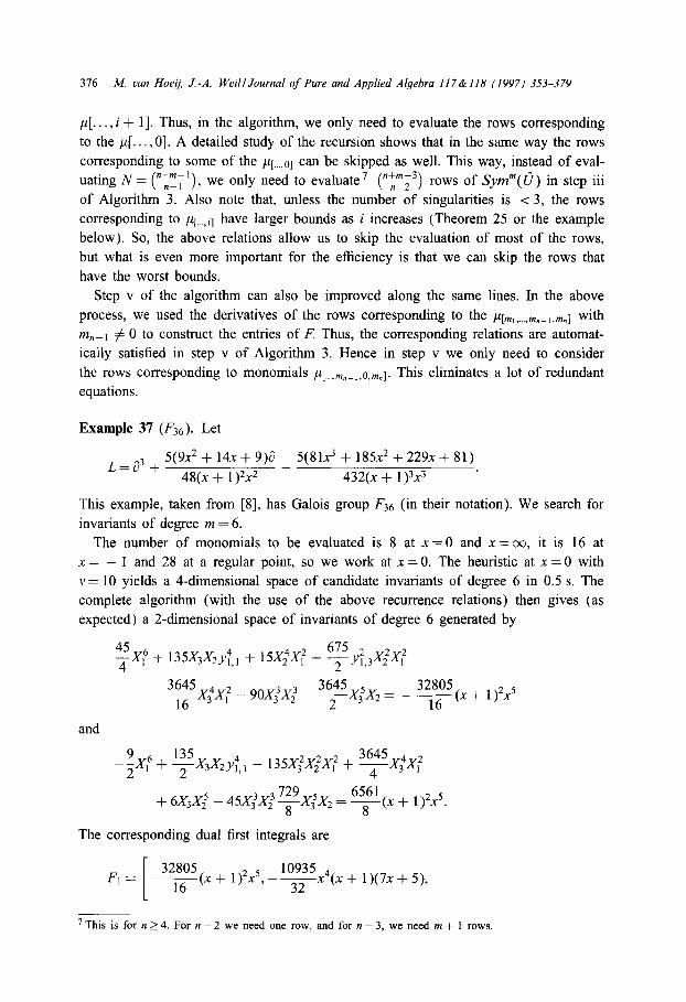
A.. ., i + I]. Thus, in the algorithm, we only need to evaluate the rows corresponding

to the ,uL[. . . ,O]. A detailed study of the recursion shows that in the same way the rows

corresponding to some of the ~1...,01 can be skipped as well. This way, instead of eval-

uating N = (“fr”; ‘) , we only need to evaluate7 (“T”y3) rows of Symm(0) in step iii

of Algorithm 3. Also note that, unless the number of singularities is < 3, the rows

corresponding to p[,,,,i] have larger bounds as i increases (Theorem 25 or the example

below). So, the above relations allow us to skip the evaluation of most of the rows,

but what is even more important for the efficiency is that we can skip the rows that

have the worst bounds.

Step v of the algorithm can also be improved along the same lines. In the above

process, we used the derivatives of the rows corresponding to the ~1,,,,,...,,,_, ,,,,I with

m,_, # 0 to construct the entries of F: Thus, the corresponding relations are automat-

ically satisfied in step v of Algorithm 3. Hence in step v we only need to consider

the rows corresponding to monomials ~[...,m,_2,0,m,1. This eliminates a lot of redundant

equations.

Example 37 (F36). Let

L = a3 + 5(9x2 + 14x + 9>a 5(81x3+185x2+229x+81)

- 48(x + 1 )2x2 432(x + 1)3x3 ’

This example, taken from [8], has Galois group F36 (in their notation). We search for

invariants of degree m = 6.

The number of monomials to be evaluated is 8 at x =0 and x = o;), it is 16 at

x = - 1 and 28 at a regular point, so we work at x =O. The heuristic at x =0 with

v = 10 yields a 4-dimensional space of candidate invariants of degree 6 in 0.5 s. The

complete algorithm (with the use of the above recurrence relations) then gives (as

expected) a 2-dimensional space of invariants of degree 6 generated by

45 4X; + 135X3X2$ I + 15X;X: + y y:, sX;X:

3645 X4X2 90~3x3 3645x3,~~ 32805 3 ’ _ 3 2 _ = _ 16 2 --g-(x + 1 )2x5

and

- ;xp + 3x2 y;‘, 135x,2x,2x: + 3645X,X, - , 4 3 ,

+ 6X3X25 - 729 6561

45X33X23 -X35X2 = 8

-+n + 1)2x?

The corresponding dual first integrals are

Fl = -F(x+ 1)‘x5,-yx4(x+ 1)(7x+5),

’ This is for n 2 4. For n = 2 we need one row, and for n = 3, we need m + 1 rows.

M. uan Hoeij, J.-A. WeillJournal of Pure and Applied Algebra 117&118 (1997) 353-379 317

1215 - =x3(-23 + 49x2 + 74x), -%x3(743 + 1463x2 + 2086x), . . . ,

5

339738624(x + 1)9x6 (258162545x3 + 8763967375~’

+ 3454336210x6 +4799496375x9 + 1442053125~‘~ + 184528125~”

+ 8908159010x7 + 430643385x* - 21 12440530x5 - 2098573250x4

- 44227701x - 23914845) 5

2717908992(x + 1 )l”x7 (2491291800x3

+ 553584375~‘~ + 30189672025~’ - 9719448300x6 + 30901623000~~

+ 16603359750~‘~ + 4702779000~” + 9196060400x7 - 804729978x2

- 7242904720x5 + 2863772665~~ - 156676680.x + 71744535) 1 6561 -$x + Q2xS, %x4(x + 1)(7x + 5)

and

F2 =

243 128~3(-55 + 89x2 + 130x), $x3(299 + 587x2 + 838x),

243x2(205x3 + 445x2 + 83x - 93)

256(x + 1) ,...,

1

1358954496(x + 1)9x6 (-1661573743x3 + 3565866895x8

+ 1902296722x6 + 3956079015x9 + 1442053125~‘~ + 184528125x”

- 1 020492670x7 - 1 846340487x2 + 12 14963 1662x’ + 90059 107 1 8x4

+ 236373147x - 23914845), 1

10871635968(x + 1)‘Ox7 (-12566581020~~

+ 553584375~‘~ + 41118775225~’ + 4173511 1940x6 + 33723573540~~

+ 17335654830~” + 4791352500~” + 42844772456~~ + 3414074670x2

+ 13326450920~~ - 21103738535~~ - 68103180x + 71744535) 1 To use the recurrence relations (*), we have to compute the rows corresponding

to monomials y’(~‘)~-~, so that makes 7 rows (instead of 28). The bounds are more

favorable for these 7 rows than for the other rows, and indeed the corresponding

7 entries of F1 and F2 are smaller expressions than most of the other entries. We

printed the first 4 entries and the 2 last entries above. One sees that the last entries are

significantly larger expressions. Precisely these large (hence: costly to compute) entries

318 M. van Hoeg, J.-A. WeillJournal of Pure and Applied Algebra 117&118 (1997) 353-379

can be skipped in step iv of Algorithm 3, as these are the entries that are given by the

recursion. This is the main reason why these relations are crucial for the efficiency.

The computation time is 36.7 s and uses 1.5 Mb of memory. We performed the same

computation without using the recursion improvements, it took 263.5s and used 2.5Mb.

We then tried the first step of the standard method (computation of L@): this took

4587 s and more than 10 Mb of memory.

5. Conclusion

We do not claim that our method is always better than the method via symmetric

powers of operators. However, we have practical evidence that this method can handle

much larger examples (and generally faster) than the previous one at our disposal.

To compute all invariants of a given equation, we now face the following open

problem: given L, can one bound the degrees of the generators of the invariant ring

(when G is reductive)? As shown in [7], a solution to this problem would yield an

algorithm for computing reductive unimodular Galois groups.

The method extends readily to systems: we then need formal solutions of systems

(e.g., via cyclic vectors); but we lose the recurrence relations that enhance the algo-

rithm, so the best there seems (surprisingly) to convert the system to an equation,

apply the above algorithms, and then perform the correct change of variables to obtain

the invariants of the original system.

We believe that the philosophy heuristic-checking is very suitable for computation.

Information on the invariants can be obtained quickly by the heuristic and by modular

arithmetic. If desired, this information can then be checked by Algorithm 3. Further-

more, Algorithm 3 provides additional useful information, namely the dual first integrals

corresponding to the invariants.

Applications of this algorithm are the computation of first integrals [26], the compu-

tation of differential relations satisfied by the solutions [7], the computation of algebraic

and Liouvillian solutions [21,23,25] and, more generally, to compute information on

the Galois group. Extensions of the above techniques to other constructions on V(L)

(and several applications) will be described in a subsequent paper.

Acknowledgements

The research of the second author was supported by the Dutch NWO-MRI (project

AIDA). The authors thank the universities of Groningen and Nijmegen as well as the

I&ole Polytechnique for their support and hospitality during the preparation of this

paper. Some computations were done on the machines of the CNRS-GDR MEDICIS

at the ficole Polytechnique.

We would like to thank Elie Compoint, Marius van der Put, Felix Ulmer, and

Michael Singer for useful remarks concerning this paper. We also thank Elie for swamp-

ing us with complicated examples that helped us with the implementation.

A4. van Hoeq, J.-A. WeillJournal of Pure and Applied Algebra 1178~118 (1997) 353-379 379

References

[l] S.A. Abramov, M. Bronstein and M. PetkoSek, On polynomial solutions of linear operators, Proc.

lSSAC’95 (ACM Press, New York, 1995).

[2] A. Barkatou, Rational Newton Algorithm for computing formal solutions of linear differential equations,

Proc. ISSAC’ (ACM Press, New York, 1988).

[3] D. Bertrand, Theorie de Galois differentielle, Cours de DEA, Notes redigees par R. Lardon, Universite

de Paris VI, 1986.

[4] D. Bertrand and F. Beukers, Equations differentielles liniaires et majorations de multiplicites, Ann.

Scient. EC. Norm. Sup. 4eme strie 18 (1985) 181-192.

[5] F. Beukers, Differential Galois theory, in: Waldschmidt, Moussa, Luck and Itzykson, eds., From Number

Theory to Physics (Springer, Berlin, 1992).

[6] E. Coddington and N. Levinson, Theory of Ordinary Differential Equations (Ma&raw-Hill, New York,

1955).

[7] E. Compoint, Equations differentielles et relations algtbriques, preprint, 1995, Universite de Paris 6.

[8] W. Geiselmann and F. Ulmer, Constructing a third order differential equation, preprint, Proc. 4th Rhine

Workshop on Computer Algebra (1996).

[9] P. Hendriks and M. van der Put, Galois action on solutions of a differential equation, J. Symbolic.

Comput. (1995).

[IO] M. van Hoeij, Formal solutions and factorization of differential operators with power series coefficients,

University of Nijmegen, Report No. 9528.

[l I] M. van Hoeij, Factorization of differential operators with rational coefficients, University of Nijmegen,

Report No. 9552.

[ 121 S. Lang, Algebra (Addison-Wesley, Reading, MA, 3rd ed., 1992).

[I31 A.H.M. Levelt, Differential Galois theory and tensor products, Indag. Math. (1989) + erratas.

[14] B. Malgrange, Sur la reduction formelle des equations differentielles a singular&es irrtgulitres,

manuscript, 1979.

[15] J. Martinet and J.P. Ramis, Gineralites sur la theorie de Galois differentielle, in: E. Toumier, ed.,

Computer Algebra and Differential Equations (Academic Press, New York, 1990).

[16] M. van der Put, Singular complex differential equations: an introduction Nieuw Achief voor Wiskunde,

4de serie 13 (3) (1995) 451-470.

[17] M.F. Singer, An outline of differential Galois theory, in: E. Toumier, ed., Computer Algebra and

Differential Equations (Academic Press, New York, 1990).

[I81 M.F. Singer, Moduli of linear differential equations on the Rieman sphere, Pac. J. Math. 160 (1993).

[ 191 M.F. Singer, Testing reducibility of linear differential operators: a group theoretic perspective, J. Appl.

Alg. Eng. Comm. Comp. 7 (1996) 77-104.

[ZO] M.F. Singer and F. Ulmer, Galois groups for second and third order linear differential equations.

J. Symbolic. Comput. 16 (1993) 1-36.

[21] M.F. Singer and F. Ulmer, Liouvillian and algebraic solutions of second and third order linear differential

equations, J. Symbolic. Comput. 16 (1993) 37-73.

[22] M.F. Singer and F. Ulmer, Necessary conditions for liouvillian solutions of (third order) linear

differential equations, J. Appl. Alg. Eng. Comm. Comput. 6 (1995) l-22.

[23] M.F. Singer and F. Ulmer, Linear diflerential equations and products of linear forms, preprint, presented

at the MEGA’ conference, Eindhoven, 6-8 June 1996.

[24] E. Toumier, Solutions formelles d’tquations differentielles, These d’Etat, Fact&C des Sciences de

Grenoble, 1987.

[25] F. Ulmer and J.A. Weil, Note on Kovacic’s algorithm prepublication IRMAR 94-13, Rennes Juillet 94,

J. Symbolic. Comput., to appear.

[26] J.A. Weil, First integrals and Darboux polynomials of homogeneous linear differential systems,

in: M. Giusti and T. Mora, eds., Proc. AAECC 11, Lecture Notes in Comp. Sci., Vol. 948 (Springer,

Berlin, 1995).

[27] J.A. Weil, Constantes et polynomes de Darboux en algtbre differentielle: application aux systemes

differentiels lineaires, Ph.D. dissertation, Ecole Polytechnique, 1995.