Variable Threshold Algorithm for Division of Labor Analyzed as a Dynamical System

Manuel Castillo-Cagigal, Eduardo Matallanas, Inaki Navarro, Estefanía Caamaño-Martín, Félix Monasterio-Huelin and Alvaro Gutiérrez

Abstract—Division of labor is a widely studied aspect of colony behavior of social insects. Division of labor models indicate how individuals distribute themselves in order to perform different tasks simultaneously. However, models that study division of labor from a dynamical system point of view cannot be found in the literature. In this paper, we define a division of labor model as a discrete-time dynamical system, in order to study the equilibrium points and their properties related to convergence and stability. By making use of this analytical model, an adaptive algorithm based on division of labor can be designed to satisfy dynamic criteria. In this way, we have designed and tested an algorithm that varies the response thresholds in order to modify the dynamic behavior of the system. This behavior modification allows the system to adapt to specific environmental and collective situations, making the algorithm a good candidate for distributed control applications. The variable threshold algorithm is based on specialization mechanisms. It is able to achieve an asymptotically stable behavior of the system in different environments and independently of the number of individuals. The algorithm has been successfully tested under several initial conditions and number of individuals.

Index Terms—Distributed control, division of labor, dynamical systems, response thresholds, swarm intelligence.

I. INTRODUCTION

SOCIETIES of insects can perform different tasks simulta­neously, distributing the workload among their individual

members. This phenomenon is called division of labor and is one of the most basic and widely studied aspects of colony behavior [1], [2]. The parallel task performance can be more efficient than the sequential task performance because the task

switching is avoided, reducing energy and time costs [3], [4]. The division of labor models indicate how individuals are distributed to perform tasks in a way appropriate to the current situation [5]. There are different classes of models based on various hypotheses about the causes of division of labor [6]. This paper focuses on the response threshold models [6]-[8].

Response threshold models operate under the assumption that individuals have internal thresholds associated to stimulus intensities. These stimuli are related to specific tasks and can be any environmental information sensed by individuals e.g., pheromone concentration or the number of encounters with other individuals [1], [9]. The probability of acting or the intensity of an action depends on the stimulus intensities and the response thresholds of the individuals [8]. Every individual has a response threshold for each possible task that it can perform [10]. Variations in stimulus intensities are caused by the task performance of the individuals [11]. Therefore, the action of the individuals modifies and is modified by the stimulus intensities, closing a loop where the stimulus intensities are the system variables.

Although collective systems are commonly studied from the dynamical systems theory perspective [12]—[15], response threshold models of division of labor focus on how the action of individuals performing one or several tasks varies in time. In contrast, this paper focuses on the study of a response threshold model of the division of labor from a dynamical systems theory point of view. This approach allows us to study the system equilibrium points and their properties related to the convergence and stability of the model [16]. In order to carry out this paper, we propose to work on a mono-task situation in discrete-time, where individuals have to decide whether they perform the task or remain inactive. The dynamical system that implements the stimulus intensity loop is based on Bonabeau et al.'s proposal [8], [11]. The study of the equilibrium points of the dynamical system is carried out with fixed response thresholds. Hence, the structure of the dynamical system does not vary in time, and the system can be reduced to a single equation.

In previous papers, some authors emphasized that stim­uli provided by the environment, as well as individual his­tory, are likely to play an important role in the structure of response threshold models [17]. These studies suggest that the response thresholds should be variable, implement­ing an adaptive process. According to this suggestion, we propose an algorithm that varies the response thresholds to

modify the dynamic behavior of the model. This behavior modification allows the system to adapt to specific environ­mental and collective situations. Several algorithms focused on the modeling of nature to modify the response thresholds can be found in the literature [6], [17]-[20]. Unlike these works, we incorporate concepts of dynamical systems in the design of the variable threshold algorithm. The proposed variable threshold algorithm, based on Theraulaz et al.'s proposal [17], is built on a specialization mechanism with a learning and a forgetting coefficient. A specialization mechanism is a reinforcement process where the likelihood to do a task increases when the task is performed and decreases when the task is not performed [1], [21]. We introduce the use of stimulus intensity and individual task performance statistics to retrieve information about the dynamical behavior of the response threshold model. These statistics are included in the proposed algorithm to modify the dynamical behavior of the model, increasing the stability and making the stimulus intensity converge to a desired value. These features have a great importance for the use of response threshold models as distributed controllers [15].

The remainder of this paper is as follows. The response threshold model and the distributed dynamical system are presented in Section II. In this section, we demonstrate the existence of four properties of the dynamical system. In Section III, the variable threshold algorithm is presented. The optimization of the configurable parameters of the variable threshold algorithm and a population study are exposed in Section IV. Finally, the conclusion, potential application, and future work are presented in Section V.

II. MODEL

In this section, we describe the response threshold model for division of labor for a single task. This model is a discrete-time stochastic process based on the stimulus intensity sensed by the individuals. We propose a transformation of the selected model into an analytical one based on the average action of the individuals. The transformation consists of representing each individual as a deterministic equation included into a discrete-time nonlinear dynamical system. Four properties of the dynamical behavior are deducted from the analytical model. These properties will help in understanding the de­velopment of the variable threshold algorithm explained in Section III.

A. Response Threshold Model

Response threshold models postulate that a task is per­formed in response to an associated stimulus intensity s e i Individuals increase their likelihood of performing a task when s exceeds their internal response threshold © e R. These models are stochastic processes because the task performance depends on the probability of acting. The relationship between the stimulus intensity and the number of individuals perform­ing the task is inversely proportional. Therefore, response threshold models implement a negative feedback loop, where s is the system variable. This study is done in the discrete-time framework and the time is denoted with subscript k. The

evolution of Sk regulates the number of individuals working on a task [22].

In this model, the performance of individual i with respect to a task at instant k is defined as a binary process represented by fk. Where fk = 0 if the individual i is not working on the task at instant k and fk = 1 on the contrary. It implies that there are not performance differences between individuals. At each instant, each individual works on the task with probability P(f¿ = 1) = p'k. Therefore, f¿ is a Bernoulli process, where the probability of acting of individual i is a function of the Sk associated with the task. Hence

Pk = T(sk, ©'') (1)

where ©' is the response threshold of individual i and T(-) is the response threshold function common to all individuals.

The response threshold functions cannot take any possible shape; they are probability functions and should represent the relationship between Sk and p'k, as previously explained. We define the following constraints for the response threshold functions: 1) T(-) e [0, 1], representing the probability of acting; 2) T(-) is a monotonically increasing function, the higher the probability of acting the higher s; 3) it must be continuous and differentiable in R; 4) the higher the slope of T(-) ( defined as T = dT/ds ) the closer ©' to s. The last constraint involves the fact that individuals become insen­sible to stimulus intensity variations far from their response thresholds. Logistic functions (e.g., Sigmoid) are examples of response threshold functions that satisfy the four constraints mentioned above.

As aforementioned, the stimulus intensity is modified by the individual task performance. The environment also produces variations in the stimulus intensity independently of whether or not the task is performed. Then, the resulting equation for discrete-time dynamics of Sk is given as follows:

sk+i=D-sk + S- Nakct (2)

where D and 5 are two constants which represent two environ­mental parameters. D represents the inertia of the environment and 5 a continuous increment of the stimulus intensity. The environment is considered to be stable and autonomous; hence D e [0, 1) and 5 e R. Nf e N is the number of individuals performing the task at instant k and it is defined as

N

1=1

where N e N is the number of individuals. Nkct introduces

the nonlinearity in (2). Nkct is a random process because it

comprises the individual actions that are themselves random processes as discussed above. In summary, (2) is the discrete-time stochastic dynamical system which defines the response threshold model of the division of labor.

B. Analytical Model

With the aim of analyzing the dynamics of the response threshold model, it is necessary to approximate (2) by an analytical equation, eliminating the random term. If Nk

ct is approximated by its expected value, the sum of individuals

task performance is approximately the sum of probabilities of acting. By combining (1), (2), and (3), the analytical model is defined as

N

Nakct « E\Nlc'] = J2 T(sk> ®') = F(sk> ®) (4)

1=1

s¡+1=D-s¡ + S-F(s¡,&) (5)

where s£ e R is the stimulus intensity at instant k for the analytical model, © is the vector of all individual response thresholds, and F(s*, ©) is the sum of all response threshold functions. The analytical model is a discrete-time deterministic dynamical system where the system variable is s*.

C. Response Threshold Model Dynamics

The study of the response threshold dynamics allows under­standing the evolution of the stimulus intensity for a certain configuration of the dynamical system. A configuration is de­fined as a fixed set of values for the environmental parameters D and 5, the response threshold functions and the response thresholds, respectively. Depending on the configuration of the dynamical system, sk can converge to a single value, perform an oscillatory behavior or respond differently to disturbances. To design the variable threshold algorithm, described in Section III, it is mandatory to define some dynamic properties of the analytical model. These properties are defined hereafter.

In the analytical model, s£ can be represented as a discrete sequence for an initial stimulus intensity SQ

[S] : s*0 , s¡ = H(sS),..., s¡= H(sl_0 (6)

H(s*) = D-s* + 8-F(s*,&) (7)

where H(s*) is the dynamic function of (5). H(s*) can be plotted as a stair-step diagram, where the y-axis is the stimulus intensity in k + 1, while the x-axis is the stimulus intensity in k. An example of a generic H(s*) function in a stair-step diagram is shown in Fig. 1(a). The evolution of s£ can be easily calculated using this diagram by the projections of H(sk) in the bisectrix, sk+i = sk, and back to H(sk+1). This graphical method is shown in Fig. 1(a), where the discrete sequence [SQ, s¡} is represented by dotted arrows.

The notion of equilibrium points is the central problem in the stability of dynamical systems [16]. The evolution of sk can be defined in relation to its equilibrium points. A point s of the nonlinear dynamic system s£+1 = H(s£) is an equilibrium point if it is a fixed point of the system (s = H(s)). Geometrically, an equilibrium point is the intersection between the function s£+1 = H(sk) and the bisectrix, s£+1 = sk. It is a constant solution because sk+1 = H(s¡) = s¡, Vk if s£ = s. The equilibrium point s of H(s*) can be observed in Fig. 1(a). Once the equilibrium points have been defined, two properties can be established.

Property 1: The slope of H(s), defined as H'(s) = dH(s)/ds, is in the range (—oo, 1).

Proof: The function H(s) is the sum of two terms which depend on s (7), hence H'{s) = D-F'(s, ©). F'(s, ©) e [0, oo) because D e [0, 1) and F(s, ©) is a continuous monotonically

sk+l

Fig. 1. Stair-step diagrams for a generic H(s*) function with D = 0 and N = 100. (a) First iteration, where s is the unique constant equilibrium point and the dotted arrows represent two steps of a stimulus intensity sequence {JQ, S¡}. (b) Five periodic equilibrium points of the second iteration.

increasing function. Therefore, it is satisfied that H'(s) e (-00,1). •

Property 2: If it exists, there is only one equilibrium point of H(s).

Proof: Let S\ be an equilibrium point of H(s). It is supposed that another equilibrium point s2 exists such that S\ i- s2- No­tice that, H(s) is continuous and differentiable because F(s, ©) is the sum of T(s, ©') which are continuous and differentiable too. Therefore, according to the Mean Value Theorem, it exists an sa e (ii, s2) such that H'(sa) = (H(s2)-H(si))/(s2-Si) = 1 which contradicts Property 1. Therefore, only one equilibrium point of H(s) is possible. •

However, the restriction of a unique constant solution does not limit the existence of multiple periodic stimulus intensity behaviors. These periodic behaviors are called periodic orbits of period T. The orbits are composed by a sequence of T stimulus intensity values repeating permanently. In this situation, it is satisfied that sk+T = sk. These periodic orbits

cannot be directly calculated from H(s*), but from the analysis of HT(s*), being the ^-iteration of the difference equation (HT = H o • • • o H). Notice that s¡+T = HT(s¡) represents the sequence {ST} : [SQ, ST, S2T, •••} and it does not include the elements of the {S} sequence between s£+T and s£. The concept of equilibrium point can also be applied to HT(s*); hence a periodic orbit is a fixed point of the iterated difference equation (Sj. = / / r ( ^ ) ) . It can also be represented graphically, plotting the function s£+T = HT(sk) and the bisectrix s£+T = s£. The equilibrium points of the second iteration of a generic function H2(s*) can be observed in Fig. 1(b). In this case, the y-axis is the k + 2 stimulus intensity. Notice that Properties 1 and 2 cannot be applied generally to HT(s*), because the slope of HT(S*) is not necessarily in the range (—oo, 1].

To know the existence and location of the equilibrium point is not enough to understand the response threshold model dynamics. An equilibrium point has different dynamic properties based on the stability when s£ takes a value close to it. An equilibrium point s is an attractor when s£ -> s for k -> oo; hence, s£ converges to this equilibrium point. An example of attractor is the equilibrium point s of Fig. 2(a). The evolution of the stimulus intensity in the analytical model can be observed using the stair-step diagram. For a s£ value close to s, s£ converges to it. The attractor concept can also be applied to periodic orbits. In Fig. 2(c), s£ converges to an oscillatory behavior for a value close to the periodic orbits of period T = 2. The attractors do not only appear in the analytical model, but also in the stochastic one. As for the randomness of the process, sk does not converge to a constant value and its variance depends on the individuals probability of acting. The evolution of sk can be observed in Fig. 2(b) and (d). In this case, it converges to the attractors of the analytical model. Therefore, it is important to analyze if the equilibrium points of the system are attractors or not, as defined in Property 3.

Property 3: If s exists and it is satisfied that \AF(sk, ©)| < (1 + D)\Ask\ ; V£ > M e N then s is an attractor. Where Ask = sk+i - sk and AF(sk, ©) = F(sk+i, ©) - F(sk, ©).

Proof: If \Ask+i\ < \Ask\ ; V ) t > M e N = > ] e > 0 such that lAifc+il < e ; V k > N > M. Hence, sequence {S} is a Cauchy sequence, being it convergent. By using (6) and (7), the previous sequence can be rewritten as

\D • Ask - AF(sk, 0 ) | < \Ask\ ; W k > M

As F(sk, ©) is a monotonically increasing function, A ^ > 0 <$• AF(sk, ©) > 0; hence, the previous inequality is satisfied if

(D - l)\Ask\ < \AF(sk, 0 ) | < (1 +D)\Ask\

The lower limit is negative because D e [0, 1), and the previous equation can be rewritten as

\AF(sk,&)\<(l+D)\Ask\

Therefore, {S} is a Cauchy sequence if \AF(sk, ©)| < (1 + D)\Ask\ ; Vk > M. According to Property 2, there is only one equilibrium point s, so {S} sequence converges to s, which is an attractor. •

The convergence of sequence [S] to s is linked to the distance between s^ and s. This distance is related to the concept of domain of attraction A(s) c M. If s0 e A(s) then it is satisfied that sk ->- s when k ->- oo. The sequence {S}, which satisfies Property 3, belongs to A(s). An example of the domain of attraction is shown in Fig. 2(a) and (c), where so e A(s) and so £ A(s), respectively. The calculation of the domain of attraction is usually either very complex or has even no analytical solution. In other cases, as the ones shown in Fig. 2(a) and (c), an analytical solution is found by means of Property 4.

Property 4: If D = 0, the domain of attraction of s of H(s) is limited by the next higher and next lower equilibrium points of H2(s).

Proof: If D = 0, according to (7)

H(s) = S - F(s, ©)

which is a monotonically decreasing function. H'(s) e (—oo, 0], Vi e R, with an unique equilibrium point s (see Property 2). According to the Chain Rule, H'm(s) = H'(Hm-\(s)) • H'm_1(s). For this reason, it is satisfied that all Hm(s) functions, with m being an odd number, are monotoni­cally decreasing, with one single equilibrium point. All Hm(s) functions, with m being an even number, are monotonically increasing. In this case, it is satisfied that s'2 < //2(s) < Hm(s) < s'2

+1. Therefore, there are no equilibrium points between [s'2, s'2

+1] and it implies that the equilibrium points of Hm(s) are the same as those of H2(s). If s is an attractor, then 0 < H'2(s) < 1. Let s+ and s~ be the next higher and next lower equilibrium point of //2W, respectively. They are unstable and for each so e (s~, s+), \sk-s\ ->- 0 when k ->- 00. Therefore, the domain of attraction of s of H(s) when D = 0 is limited by s+ and s~. •

Once s£ has converged to an equilibrium point or periodic orbit, it stays in this state indefinitely. The response threshold model dynamics can vary the equilibrium point in which it is operating if s£ takes a value in other domain of attraction. This s£ modification can be obtained through an external disturbance. This event would modify the stimulus intensity evolution permanently.

To represent the disturbances mathematically, we use the nonlinear function Kronecker delta 4- /- This function is 1 if k = I, and 0 otherwise. 4 - / is a nonpermanent stimulus intensity disturbance which occurs at time instant I. It is inserted in the response threshold model dynamics as follows:

s¡+l=H{skk) + ai-h-i (8)

where a¡ is the disturbance amplitude at instant l. s¡, can converge to another equilibrium point depending on a¡ and the size of the domain of attraction of the equilibrium point in which the response threshold dynamics is operating. An example with two disturbances can be observed in Fig. 3(a). In this example, SQ is in the domain of attraction of s; hence, s£ converges to this equilibrium point. The first disturbance takes place at k = 50 and it displaces the stimulus intensity out of A(s). This behavior causes that the stimulus intensity diverges from s and converges to a periodic orbit. The second

Sfc

"s

s+] A(l)

s-l A ^t\ í - A « s+

'/H2(s

H(s

*í

(a) (b)

Fig. 2. Evolution of stimulus intensity for a generic H(s*) function with D = 0 and W = 100 and for different initial values, (a) Stair-step diagram for so £ A(s). (b) Evolution of the stochastic model for SQ S A(S). (C) Stair-step diagram for SQ £ A(s). (d) Evolution of the stochastic model for SQ £ A(s). Domains of attraction are represented by their upper (s+) and lower (j~) values.

Sfc+l>Sfc+2

Sk

s:

s- A(s) s+

(a)

l50<5fc-50 fll00¿fc-100

Fig. 3. Disturbance effects example with two disturbances a¡o • 4-50 a nd "loo • &k-loo f° r a generic H(s*) function with D = 0 and W = 100. (a) Representation of disturbances in the analytical model, (b) Evolution of the stimulus intensity in the stochastic model.

disturbance takes place at k = 100 and it returns the stimulus intensity to the domain of attraction of s. The evolution of Sk for the stochastic model is shown in Fig. 3(b) with similar dynamic properties to the analytical one.

III. VARIABLE THRESHOLD ALGORITHM

A dynamical system can be designed to perform specific dynamic behaviors, e.g., ensure that Sk converges asymptot­ically to a concrete value. The downside of this procedure

is that it is necessary to know the environmental parameters when the system is designed. If environmental parameters are not known, the dynamical behavior of the response threshold model cannot be ensured. In this case, the response thresholds should be modified in real time, adapting to the environment. In this section, we propose a variable threshold algorithm which ensures the convergence of the stimulus intensity to a certain value without the need to know the environmental parameters. The variable threshold algorithm modifies the re­sponse thresholds in a distributed manner. There is no explicit information exchange between individuals. Through the eval­uation of their own work and Sk, the individuals modify their response thresholds and hence, the dynamical system behavior.

The variable threshold algorithm takes into account the response threshold dynamics properties and has the following features.

1) Stability against disturbances: The presence of stimulus intensity disturbances (ak-&k) can modify the equilibrium point in which the dynamical system is operating. It implies that Sk evolution varies in a qualitative point of view, e.g., from a nonoscillatory behavior to an oscillatory one. The objective of the variable threshold algorithm is to stabilize the response threshold dynamics in a concrete equilibrium point, in such a way that the disturbances cannot get Sk out of it.

2) Oscillatory behavior avoidance: If the system is op­erating in a periodic orbit, Sk varies periodically. The objective of the variable threshold algorithm is to con­verge asymptotically to a concrete value and therefore oscillatory behaviors must be avoided.

3) Reference stimulus intensity: Although Sk converges asymptotically to a stable equilibrium point, the value of this equilibrium point is not guaranteed. The objective of the variable threshold algorithm is to make sk converge to a reference value.

A. Stability Against Disturbances

Every dynamical system that faces a real environment must take into account the presence of disturbances. Variations of Sk induced by disturbances can modify the evolution of Sk permanently, as explained in Section II. This effect should

be avoided by the variable threshold algorithm. Permanent modifications of sk evolution arise when sk takes a value in a domain of attraction of another equilibrium point. Hence, the permanent modifications induced by disturbances can be avoided if the domain of attraction, where the stimulus intensity is located, increases.

Conjecture 1: The farther the response thresholds from s are, the greater the domain of attraction of s is. Reasoning: As for the definition of the response threshold function, T'(s, ©') is reduced in a region close to s if the distance between ©' and s is increased. F'(s, ©) is reduced if the response thresholds increase their distance from s, because F(s, ©) is the sum of the individual response threshold functions. It implies that the difference AF(sk, ©) for two points sk and Sk+i that belongs to a region close to s, decreases as far as the response thresholds from s are. Therefore, if the response thresholds tend to increase their distances with respect to s, the region in which the sequence {Sk} satisfies the inequality of Property 3 increases.

In order to implement Conjecture 1, the variable threshold algorithm is based on a specialization mechanism. Specializa­tion is a postulated mechanism in which the more often an individual performs a task, the more often it continues doing the same task with a higher probability [17]. In a specialization process, some individuals tend to do always the same task while others never do it (p\ «a 1 or p'k «a 0, V£ respectively); when this occurs, individuals are specialized. In the response threshold models, the response threshold decreases when the corresponding task is performed and vice versa, implementing a positive feedback loop and increasing the distance between the response thresholds and s. The response threshold variation A©[ of the individual i at instant k is defined by the following nonlinear equations

(9) ©*+i = ©1 + A0¿

A©! " P i + 3 if / t = l

(10)

where <p'k is the learning coefficient which implements the specialization and f¿ is the forgetting coefficient which im­plements the opposite process to specialization. Note that the response threshold modification depends on the task perfor­mance of individual i. It implies that if an individual works on the task, its response threshold is reduced by increasing its probability of acting. On the contrary, if an individual does not work on the task, its response threshold is increased reducing its probability of acting.

When an individual is specialized, the learning coefficient continues increasing (or decreasing) the response threshold indefinitely, so it satisfies \&'k - ^1 -* °o when k -> oo. According to the definition of the response threshold function, it implies that T'(sk, &'k) -> 0. Therefore, the individuals become insensible to Sk variations and continue doing always the same action; this phenomenon is called overspecialization. This situation has been solved in previous papers limiting the response threshold values in a certain range. In this paper, we propose the use of a continuous function to control the

response threshold variations. The necessary information to perform this feature can be locally obtained from the following two stimulus intensity statistics: Sk that is the exponential moving average of sk and ak that is the exponential moving variance of sk. Hence

Sk = psk + (l - p)Sk-\

<yk = p{sk - sk) + (l - p ) f f n

( i i )

(12)

Both time-dependent variables take into account the current stimulus value and its previous history, p is a configurable parameter which represents the weight of new samples in relation with the historical one. As p e [0,1], the higher p is, the more relevant current values are and vice versa. Then, a new property can be enunciated to define the control function as:

Property 5: When the stimulus intensity has converged to s, the lower the variance is, the greater the distance between response thresholds and s is.

Proof: Consider the variance of Nk as

Var[Nkct]

N N

E ^ 1 - Pk) = J2T^ ©x1 - T^ ©'')) 1=1 =i

where the definition of the response threshold function, T(-) -> 0 or 1 when | ^ - ©'| -> oo and T(-) -> 0.5 when \sk - ©'| -> 0. Therefore, T(-)(l - T(-)) -> 0 when \s - ©''| -> oo and T(-)(l - T(-)) -> 0.25 when \s - ©'| -> 0, which is the maximum value. Let £2 be a vector of response thresholds ©' e £2 and <t> another vector of response thresh­olds & e <P such that \s - &'\ < \s - ®>\. Therefore, T(sk, ©'XI - T(sk, ©'')) > T(sk, ©0(1 - T(sk, &)) Vi and Var[Nk

ct]a > Var[N£c>]<t,. It means that the greater the distance of the response threshold to the equilibrium point is, the lower the variance is. •

Conjecture 1 together with Property 5 establish ak as an indicator of the domain of attraction and the overspecialization of the individuals. If the response thresholds are close to the equilibrium point, ak increases. On the other hand, if the individuals are overspecialized then ak ->- 0. The variable threshold algorithm has to reach a compromise between the stability and the overspecialization. Following this compro­mise, cpk and §t can be defined as

<Pk = vk-e

lk = ea

Vk = (1 +CtlJok)

\Sk-&k\

Vk (13)

(14)

(15)

where vk denotes the standard deviation of sk. Note that cpk

decreases when the distance between the stimulus intensity and the threshold value increases; hence, it avoids overspe­cialization. The higher vk is, the higher the distance between sk and &'k is, because the exponential index of cpk is inversely proportional to vk. Moreover, the magnitude of the learning coefficient is directly proportional to vk which implies that the higher ak is, the higher the learning step is. a\ is a configurable

0

,

e„

©o

= 45

= 10

* • =

<

50 k (a)

i = 50 (b)

Fig. 4. Variable threshold algorithm example for so S A(s) with D = 0, S = 100, and N = 100 with 80% of individuals having 9 0 = 10 and 20% having 0o = 45. (a) Evolution in time of response thresholds, (b) Evolution of stimulus intensity and domain of attraction limits (s~, s+).

Fig. 5. Variable threshold algorithm example for so £ A(s) with D = 0, S = 100, and N = 100 with 80% of individuals having 9 0 = 10 and 20% having 0o = 45. (a) Evolution in time of response thresholds, (b) Evolution of stimulus intensity and domain of attraction limits (s~, s+).

parameter which regulates the effect ofok in <pk. The forgetting coefficient is the opposite to the learning one; hence, the higher this term is the lower ak is, avoiding overspecialization. a2 is a configurable parameter which regulates the effect of ak in f¿.

An example of the variable threshold algorithm is shown in Fig. 4. In this example, the environmental parameters are D = 0 and 5 = 100. The population of individuals is N = 100, where 80 individuals have an initial response thresh­old &0 = 10 and 20 individuals ©j, = 45. The H(s, ©) function of the dynamical system was already plotted in Fig. 1(a). so is in the domain of attraction of the asymptotically stable equilib­rium point (so e A(s)). During the first time steps (k < 50), the variable threshold algorithm is not acting; hence, the response thresholds maintain the same value as observed in Fig. 4(a). In the time step k = 50, the variable threshold algorithm is activated and it modifies the response thresholds. The distance between the response thresholds and the asymptotically stable equilibrium point is increased, because of the variance of the stimulus intensity. Moreover, ak is reduced and the domain of attraction is increased, as can be observed in Fig. 4(b).

B. Oscillatory Behavior Avoidance

We propose another example to show the effect of os­cillatory behavior in Fig. 5. The environmental parameter, the number of individuals, and the response thresholds initial values are the same as those in the previous experiment. In this example, the initial stimulus intensity is not in the domain of attraction of the asymptotically stable equilibrium point (io ^ Ms)). As in the previous example, the variable threshold

algorithm is activated at time step k = 50. In this situation, the algorithm cannot drive sk to a nonoscillatory solution [see Fig. 5(b)]. Fig. 5(a) shows how the response threshold values are modified, performing an oscillatory behavior.

An oscillatory behavior implies that several individuals are changing permanently their task performance f¿. Individuals that carry out these oscillations are sensing different stim­ulus intensity values, lower and higher than their response thresholds, and they provoke that the probability of acting switches between a high and a low value. Therefore, the response thresholds of the individuals which are performing an oscillatory behavior are between the stimulus intensity values.

As shown in the previous example, the specialization mech­anism is not able to avoid oscillations in its actual form. Os­cillations can be avoided by using individual task performance information. Let the exponential moving average (f¿) of the action of the individual i be defined as

fi = pfi + o.-P)fU (16)

where p is the same configurable parameter of (12). f¿ e [0, 1] because f¿ is a binary variable. f¿ takes the value 0 or 1 when an individual is specialized because it tends to do the same action, while fk ->- 0.5, when there is high variability of the individual task performance.

Let the stress factor be defined as

%=4-/¿(l-/¿) (17)

where r¡k e [0, 1]. For the individuals that are not performing an oscillatory behavior r¡k ->- 0 and for the individuals that

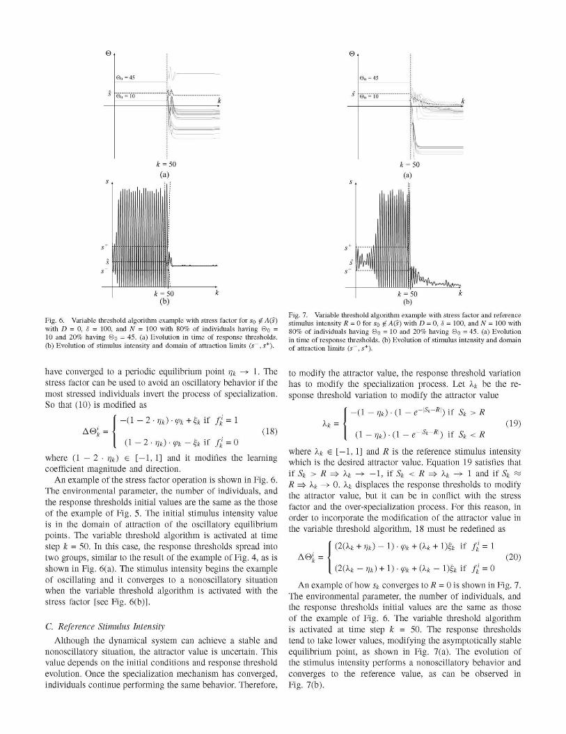
Fig. 6. Variable threshold algorithm example with stress factor for so £ A(s) with D = 0, S = 100, and N = 100 with 80% of individuals having 9 0 = 10 and 20% having 0o = 45. (a) Evolution in time of response thresholds, (b) Evolution of stimulus intensity and domain of attraction limits (s~, s+).

Fig. 7. Variable threshold algorithm example with stress factor and reference stimulus intensity R = 0 for s0 i A(s) with D = 0,S = 100, and N = 100 with 80% of individuals having 0o = 10 and 20% having 0o = 45. (a) Evolution in time of response thresholds, (b) Evolution of stimulus intensity and domain of attraction limits (s~, s+).

have converged to a periodic equilibrium point r\k -> 1. The stress factor can be used to avoid an oscillatory behavior if the most stressed individuals invert the process of specialization. So that (10) is modified as

AQ>k=\ -(1 - 2-ifc) •«£>*+& if fl = \

(\-2-r)k)-<Pk-htt fi = o (18)

where ( 1 - 2 - % ) e [—1,1] and it modifies the learning coefficient magnitude and direction.

An example of the stress factor operation is shown in Fig. 6. The environmental parameter, the number of individuals, and the response thresholds initial values are the same as the those of the example of Fig. 5. The initial stimulus intensity value is in the domain of attraction of the oscillatory equilibrium points. The variable threshold algorithm is activated at time step k = 50. In this case, the response thresholds spread into two groups, similar to the result of the example of Fig. 4, as is shown in Fig. 6(a). The stimulus intensity begins the example of oscillating and it converges to a nonoscillatory situation when the variable threshold algorithm is activated with the stress factor [see Fig. 6(b)].

C. Reference Stimulus Intensity

Although the dynamical system can achieve a stable and nonoscillatory situation, the attractor value is uncertain. This value depends on the initial conditions and response threshold evolution. Once the specialization mechanism has converged, individuals continue performing the same behavior. Therefore,

to modify the attractor value, the response threshold variation has to modify the specialization process. Let A* be the re­sponse threshold variation to modify the attractor value

At = - ( ! - % ) • ( !

( ! - % ) • ( ! - - I * -

-ff|) if Sk > R

R]) if Sk<R (19)

where Xk e [-1,1] and R is the reference stimulus intensity which is the desired attractor value. Equation 19 satisfies that if Sk > R =>• h -> - 1 , if Sk < R =>• h -> 1 and if Sk «= R =>• A* ->- 0. A.*; displaces the response thresholds to modify the attractor value, but it can be in conflict with the stress factor and the over-specialization process. For this reason, in order to incorporate the modification of the attractor value in the variable threshold algorithm, 18 must be redefined as

A©! (2(A* + m) - ! ) • % + (A* + 1)& if fl = 1

(2(xk - r¡k) + i)-<pk + (h - i)& if fl = o (20)

An example of how sk converges to R = 0 is shown in Fig. 7. The environmental parameter, the number of individuals, and the response thresholds initial values are the same as those of the example of Fig. 6. The variable threshold algorithm is activated at time step k = 50. The response thresholds tend to take lower values, modifying the asymptotically stable equilibrium point, as shown in Fig. 7(a). The evolution of the stimulus intensity performs a nonoscillatory behavior and converges to the reference value, as can be observed in Fig. 7(b).

aj = 10'

I1

(a)

a2 = 105

I 1

(b)

Fig. 8. Grayscale color-map where the darker the shorter convergence time. It represents the Qs of convergence time for the exhaustive search of the configurable parameters of the variable threshold algorithm (see Section III), (a) Scanning of p and ci\ for a?2 = 101. (b) Scanning of p and a\ for a?2 = 10 • (c) Scanning of p and a\ for a?2 = 1020.

IV. EXPERIMENTS

In this section, we propose a set of experiments to optimize the variable threshold parameters and to test them with dif­ferent populations. As described in Section III, the variable threshold algorithm has three configurable parameters: p, a\, and a2. They modify how the variable threshold algorithm adapts to the environment to achieve the previously defined dynamic behavior. This algorithm can be optimized following a certain criterion. An exhaustive search of these parameters has been carried out to locate the minimum convergence time.

The response threshold function used for the experiments is the Sigmoid function

r(ft .Q '>=1 + g-LeO <21> where j3 = -0.2 for all individuals. Using this response threshold function, simulations with different environment and initial configurations have been performed. In the exhaustive search, every combination of p, a\, and a2 has been clustered in a set. Every set of these parameters has been simulated for populations of 102, 103, and 104 individuals. Moreover, each of these populations has been simulated for two values of coefficient D, 0 and 1. 5 has been fixed to N/2. The reference stimulus intensity has been fixed toR = 0. The initial stimulus intensity value has been set to so = 8. Initial response threshold values have also been tested, initializing the response thresholds with two uniform probability distributions between [—Af, 0] and [0, A7]. These distributions have been chosen to provoke asymmetric situations with respect to R. Moreover, because of the pseudo random nature of the experiments, each configuration has been simulated for 30 different seeds of a random generator number. Therefore, 360 simulations have been performed for every set of p, a\, and a2, calculating the convergence time (Tc) for every simulation.

It is considered that the system has converged when the fol­lowing two constraints are satisfied: 1) The stimulus intensity mean or second quartile (Q2) is between [R -1, R +1], the first quartile (gi) is between [R - 2, K], and the third quartile (Q3) is between [R,R + 2]. This convergence constraint operates as a mean filter, removing the noise of the stochastic process and ensuring the convergence to the reference stimulus intensity R.

2) The stimulus intensity variance is in [0.5, 2.0]. The lower limit indicates that the individuals are not overspecialized and the upper one indicates a minimum distance between the response thresholds and the attractor.

To analyze the effects of the configurable parameters on Tc, several sets of these parameters have been simulated. Every set is a different combination of p, a\, and a2. Each parameter is discretized in a certain range with an interval between values, such that, p e [0, 1] with an interval of 0.01, a\ e [0, 10] with an interval of 0.1 and a2 e [1, 1020] with a logarithmic interval of 10. This combination produces 2 • 105 different sets of configurable parameters. As aforementioned, 360 simulations have been performed for every set and this leads to 72 • 106

simulations for the exhaustive search campaign. The third quartile of the convergence time is shown in

Fig. 8 with color maps. Each color map has been plotted for a fixed value of a2 and represents the scanning of p and a\. The values of the parameters and the convergence time have a nonlinear relationship because the shape of the color map. Although a2 has been simulated for more values than shown, the more representative ones have been selected. The optimum value of a2 is 105 whose color map is shown in Fig.8(b). A lower value (a2 = 101) and a upper value (a2 = 1020) than the optimum one are plotted in figures 8(a) and (c), respectively. The minimum convergence time in Q¡ is found for p = 0.64, a\ = 2.0 and a2 = 105.

Finally, a study of the effects on convergence time (7c) for different population sizes has been carried out. For each population size, the study has been divided for D = 0 and D «a 1, which is a set [N, D}. For each set [N, D), several simulations have been carried out. The response threshold functions, 5, s0, and R in each simulation are the same as the exhaustive search. Different initial response thresholds values have also been simulated with uniform distributions between [—A7,0] and [0,N]. The number of seeds of the random number generator has been set to 100, to have enough samples for a statistical comparison. Therefore, there are 400 simulations for every set [N, D}. The results of these simulations are shown in Fig. 9. The convergence times of all studied sets [N, D} are represented through box-plots. The Tc increases approximately linearly with a logarithmic

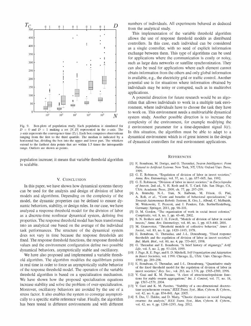
101 102 103 104 105

Fig. 9. Box-plots of population study. Each population is simulated for D = 0 and D = 1 making a set {N, D] represented in the x-axis. The y-axis represents the convergence time (7c). Each box comprises observations ranging from the first to the third quartile. The median is indicated by a horizontal bar, dividing the box into the upper and lower part. The whiskers extend to the farthest data points that are within 1.5 times the interquartile range. Outliers are shown as points.

numbers of individuals. All experiments behaved as deduced from the analytical study.

This implementation of the variable threshold algorithm allows the use of response threshold models as distributed controllers. In this case, each individual can be considered as a single controller, with no need of explicit information exchange between them. This type of algorithms can be used for applications where the communication is costly or noisy, such as large data networks or satellite synchronization. They can also be used for applications where each element cannot obtain information from the others and only global information is available, e.g., the electricity grid or traffic control. Another potential use is for situations where information obtained by individuals may be noisy or corrupted, such as in multirobot applications.

A potential direction for future research would be an algo­rithm that allows individuals to work in a multiple task envi­ronment, where individuals have to choose the task they have to work on. This environment needs a multivariable dynamical system study. Another possible direction is to increase the complexity of the environment, for example modifying the 5 environment parameter for a time-dependent signal S(t). In this situation, the algorithm must be able to adapt to a dynamical environment which is of great interest in the design of dynamical controllers for real environment applications.

population increase; it means that variable threshold algorithm is scalable.

V. CONCLUSION

In this paper, we have shown how dynamical systems theory can be used for the analysis and design of division of labor models and algorithms. Depending on the complexity of the model, the dynamic properties can be defined to ensure dy­namic behaviors, stability, or design rules. In our case, we have analyzed a response threshold model for the division of labor as a discrete-time nonlinear dynamical system, defining five properties. The response threshold model has been transformed into an analytical one based on the average of the individual task performances. The structure of the dynamical system does not vary in time because the response thresholds are fixed. The response threshold functions, the response threshold values and the environment configuration define two possible dynamical behaviors, asymptotically stable and oscillatory.

We have also proposed and implemented a variable thresh­old algorithm. The algorithm modifies the equilibrium points in real time in order to force an asymptotically stable behavior of the response threshold model. The operation of the variable threshold algorithm is based on a specialization mechanism. We have shown how the proposed specialization equations increase stability and solve the problem of over-specialization. Moreover, oscillatory behaviors are avoided by the use of a stress factor. It also enables the system to converge asymptoti­cally to a specific stable reference value. Finally, the algorithm has been tested in different environments and with different

REFERENCES

[1] E. Bonabeau, M. Dorigo, and G. Theraulaz, Swarm Intelligence: From Natural to Artificial Systems. New York, NY, USA: Oxford Univ. Press, 1999.

[2] G. E. Robinson, "Regulation of division of labor in insect societies," Annu. Rev. Entomology, vol. 37, no. 1, pp. 637-665, Jan. 1992.

[3] G. E. Robinson, "Division of labor in insect societies," in Encyclopedia of Insects, 2nd ed., V. H. Resh and R. T. Card, Eds. San Diego, CA, USA: Academic Press, 2009, ch. 77, pp. 297-299.

[4] A. Brutschy, N.-L. Tran, N. Baiboun, M. Frison, G. Pini, A. Roli, et al., "Costs and benefits of behavioral specialization," in Towards Autonomous Robotic Systems, R. Gro, L. Alboul, C. Melhuish, M. Witkowski, T. Prescott, and J. Penders, Eds. Berlin/Heidelberg, Germany: Springer, 2011, pp. 90-101.

[5] D. M. Gordon, "The organization of work in social insect colonies," Complexity, vol. 8, no. 1, pp. 43-46, 2002.

[6] S. N. Beshers and J. H. Fewell, "Models of division of labor in social insects," Annu. Rev. Entomology, vol. 46, no. 1, pp. 413-440, 2001.

[7] M. Granovetter, "Threshold models of collective behavior," Amer. J. Social, vol. 83, no. 6, pp. 1420-1443, 1978.

[8] E. Bonabeau, G. Theraulaz, and J.-L. Deneubourg, "Fixed response thresholds and the regulation of division of labor in insect societies," Bui. Math. Biol, vol. 60, no. 4, pp. 753-807, 1998.

[9] G. Theraulaz and E. Bonabeau, "A brief history of stigmergy," Artif. Life, vol. 5, no. 2, pp. 97-116, 1999.

[10] J. Page, R. E. Page, and S. D. Mitchell, Self Organization and Adaptation in Insect Societies, vol. 1 990. Chicago, IL, USA: Univ. Chicago Press, 1990, pp. 289-298.

[11] E. Bonabeau, G. Theraulaz, and J.-L. Deneubourg, "Quantitative study of the fixed threshold model for the regulation of division of labor in insect societies," Roy. Soc, vol. 263, no. 1 376, pp. 1565-1569, 1996.

[12] V. Gazi and K. M. Passino, "A class of attractions/repulsions func­tions for stable swarm aggregations," Int. J. Control, vol. 77, no. 18, pp. 1567-1579, 2004.

[13] V. Gazi and K. M. Passino, "Stability of a one-dimensional discrete-time asynchronous swarm," IEEE Trans. Syst., Man, Cybern. B, Cybern., vol. 42, no. 6, pp. 834-841, Apr. 2005.

[14] S. Das, U. Haider, and D. Maity, "Chaotic dynamics in social foraging swarms: An analysis," IEEE Trans. Syst., Man, Cybern. B, Cybern., vol. 42, no. 4, pp. 1288-1293, Aug. 2012.

[15] G. Antonelli, "Interconnected dynamic systems: An overview on dis­tributed control," IEEE Trans. Syst., Man, Cybern. B, Cybern., vol. 33, no. 1, pp. 76-88, Feb. 2013.

[16] J. Guckenheimer and P. Holmes, Nonlinear Oscilations, Dynamical Sys­tems and Bifurcations of Vector Fields. New York, NY, USA: Springer, 1983.

[17] G. Theraulaz, E. Bonabeau, and J.-L. Deneubourg, "Response threshold reinforcement and division of labor in insect societies," Roy. Soc, vol. 265, no. 1393, pp. 327-332, 1998.

[18] E. Bonabeau, A. Sobkowski, G. Theraulaz, and J.-L. Deneubourg, "Adaptive task allocation inspired by a model of division of labor in social insects," in Proc. BCEC97, 1997, pp. 36-45.

[19] A. J. Spencer, I. D. Couzin, and N. R. Franks, "The dynamics of specialization and generalization within biological populations," Adv. Complex Syst., vol. 1, no. 1, pp. 1-14, 1998.

[20] M. Campos, E. Bonabeau, G. Theraulaz, and J.-L. Deneubourg, "Dy­namic scheduling and division of labor in social insects." Adapt. Behav., vol. 8, no. 2, pp. 83-95, 2000.

[21] R. S. Sutton and A. G. Barto, Reinforcement Learning: An Introduction. Cambridge, MA, USA: MIT Press, 1998.

[22] S. Gamier, J. Gautrais, and G. Theraulaz, "The biological principles of swarm intelligence," Swarm Inteli, vol. 1, no. 1, pp. 3-31, 2007.

Manuel Castillo-Cagigal received the M.Sc. degree in telecommunication engineering from the Univer­sidad de Málaga (UMA), Málaga, Spain, in 2009, and the M.Sc. degree in photovoltaic solar energy from the Universidad Politécnica de Madrid (UPM), Madrid, Spain, in 2010, where he is currently a Ph.D. student in the area of control and energy management with ETSI de Telecomunicación.

In 2013, he was a Visiting Researcher with the Institut de Recherches Interdisciplinaires et de Développements en Intelligence Artificielle, Uni-

versité Libre de Bruxelles, Brussels, Belgium. He has authored and co-authored five international journal papers and eight conference proceeding. His current research interests include swarm intelligence, control systems, sensors networks, and demand-side management applications specially focused on smart-grids and renewable energies.

Eduardo Matallanas received the M.Sc. degree in electronic engineering and the M.Sc. degree in photovoltaic solar energy from the Universidad Politécnica de Madrid, Madrid, Spain, in 2010 and 2011, respectively, where he is currently pursuing the Ph.D. degree in the area of control and energy management with ETSI de Telecomunicación and Instituto de Energía Solar.

He has authored and co-authored four international journal papers and five refereed conference proceed­ing. His current research interests include swarm

intelligence, artificial intelligence, neuroscience, control systems, sensors networks, and demand-side management applications especially focused on smart grids and renewable energies.

I Iñaki Navarro was born in Madrid, Spain, in 1980. He received the M.Sc. degree in telecommunication engineering and the Ph.D. degree in robotics and automation from Univesidad Politécnica de Madrid (UPM), Madrid, in 2004 and 2010, respectively.

In 2012, he was a Post-Doctoral Researcher with I ETSI de Telecomunicación, UPM. Since 2013, he I has been a Post-Doctoral Fellow with the Dis-I tributed Intelligent Systems and Algorithms Labo-I ratory, Ecole Polytechnique Fedérale de Lausanne,

Lausanne, Switzerland. He has authored and co-authored various international journal articles, and several book chapters and refereed conference papers. His current research interests include formation control of mobile robots, swarm robotics, distributed consensus of agents and mobile robotics, sensor monitoring, machine learning, and robot learning.

Estefanía Caamaño Martín received the degree in telecommunications engineering and the Ph.D. degree in telecommunications engineering from the Universidad Politécnica de Madrid (UPM), Madrid, Spain, in 1994 and 1998, respectively.

She is a Researcher with Solar Energy Institute, UPM, in the field of photovoltaic systems, and is an Associate Professor of electronics technology with ETSI de Telecomunicación, UPM. She is an author and co-author of 12 book chapters, 15 refereed journal papers, and over 45 conference proceeding

papers. Her current research interests include photovoltaic distributed genera­tion especially focused on urban environments from architectural and electrical energy perspectives.

Félix Monasterio-Huelin received the Ph.D. degree from the Universidad Politécnica de Madrid (UPM), Madrid, Spain, in 1987.

He is currently a Professor with the ETSI de Tele­comunicación, UPM. His current research interests include field of intelligent robotics, neural networks, automatic control, and haptic devices.

Alvaro Gutiérrez (S'99-M'08-SM'12) received the M.Sc. degree in electronic engineering and the Ph.D. degree in computer science from the Universidad Politécnica de Madrid (UPM), Madrid, Spain, in 2004 and 2009, respectively.

He was a Visiting Researcher with the Institut de Recherches Interdisciplinaires et de Développements en Intelligence Artificielle, Université Libre de Brux­elles, Brussels, Belgium in 2008. He is currently an Associate Professor of automatic and control systems with ETSI de Telecomunicación, UPM. He

has authored and co-authored three book chapters and over 35 refereed journal papers and conference proceeding papers. His current research interests include swarm robotics, control systems, sensor networks, and demand-side management applications specially focused on smart-grids and renewable energies.