Case Study Methodology to Monitor & Evaluate Community ......case : study : study : to : to

Value Based Methodology to Evaluate Sensors for Bridge Structural Health
Monitoring Systems
by
JEFFERSON SANTOS DE OLIVEIRA
A thesis submitted to
Florida Institute of Technology
in partial fulfillment of the requirements
for the degree of
Master of Science
in
Systems Engineering
Melbourne, Florida
August, 2016

We the undersigned committee hereby approve the attached thesis, “Value Based
Methodology to Evaluate Sensors for Bridge Structural Health Monitoring
Systems” by Jefferson Santos de Oliveira.
_________________________________________________
Luis Daniel Otero, Ph.D. (Major Advisor)
Associate Professor, Department of Engineering Systems
College of Engineering
_________________________________________________
Aldo Fabregas, Ph.D.
Assistant Professor, Department of Engineering Systems
College of Engineering
_________________________________________________
Munevver Subasi, Ph.D.
Associate Professor, Department of Mathematical Sciences
College of Science
_________________________________________________
Muzaffar A. Shaikh, Ph.D.
Professor and Head, Department of Department of Engineering
Systems, College of Engineering
iii
Abstract
Title: Value Based Methodology to Evaluate Sensors for Bridge Structural Health
Monitoring Systems
Author: Jefferson Santos de Oliveira
Advisor: Luis Daniel Otero, Ph. D.
Structural health monitoring (SHM) systems have become important tools in the
transportation industry to help monitor the behavior and health of civil structures. Today,
there is a real concern about the health of bridges because these structures are aging, and
various failure events have contributed to increase that concern. Consequently, the topic of
improving the effectiveness and appropriate use of SHM systems have become the focus of
various government agencies and researchers, both in industry and academia. In this
context, this thesis work was developed to understand the general components of bridge
SHM systems, and present a methodology to help decision-makers prioritize a set of
sensors to be selected for a particular SHM system to satisfy specific mission objectives.
This thesis presents a value based approach to prioritize sensors, developing concepts of
qualitative value model, quantitative value model, and the swing weight matrix method to
yield a ranked list of sensor alternatives to choose from in order to build an SHM system
for bridge inspection purposes. Sensitive analyses were also conducted to evaluate the
robustness of the methodology presented in the thesis.

iv
Table of Contents
Abstract ................................................................................................................... iii
Table of Contents ................................................................................................... iv
List of Figures ......................................................................................................... vi
List of Tables ......................................................................................................... vii
Acknowledgement ................................................................................................ viii
Dedication ............................................................................................................... ix
Chapter 1 Introduction ............................................................................................ 1 1.1. Research Context ...................................................................................................... 1 1.2. Objectives .................................................................................................................. 1 1.3. Overview of the Thesis ............................................................................................. 2
Chapter 2 Review of Structural Health Monitoring of Bridges .......................... 3 2.1. Introduction .............................................................................................................. 3 2.2. Definitions of Bridge Health Monitoring ............................................................... 7 2.3. Types of Monitoring ................................................................................................. 9
2.3.1. Time Frame ......................................................................................................... 9 2.3.2. Scale .................................................................................................................. 10
2.4. Damage Detection Methodologies ......................................................................... 11 2.4.1. Non-Destructive Testing and Evaluation Methods ........................................... 12 2.4.1.1. Visual Inspection............................................................................................ 12 2.4.1.2. Ultrasonic Method.......................................................................................... 13 2.4.1.3. Acoustic Emission Method ............................................................................ 13 2.4.2. Vibration Based Methods .................................................................................. 14 2.4.2.1. Resonant Frequency ....................................................................................... 15 2.4.2.2. Mode Shape Changes ..................................................................................... 16 2.4.2.3. Dynamic Flexibility Matrix ........................................................................... 17 2.4.3. Pattern Recognition Methods ............................................................................ 18
2.5. Structural Health Monitoring Components ......................................................... 19 2.5.1. Sensory System ................................................................................................. 20 2.5.2. Data Acquisition System ................................................................................... 21 2.5.3. Data Transmission System ................................................................................ 21 2.5.4. Data Processing and Analysis System .............................................................. 22 2.5.5. Data Management System ................................................................................ 23

v
2.6. Sensors Used in Structural Health Monitoring ................................................... 24 2.6.1. Accelerometers.................................................................................................. 24 2.6.1.1. Piezoelectric Accelerometers ......................................................................... 25 2.6.1.2. Capacitive Accelerometers ............................................................................ 26 2.6.1.3. Piezoresistive Accelerometer ......................................................................... 26 2.6.1.4. Servo Accelerometer ...................................................................................... 27 2.6.2. Strain Gauges .................................................................................................... 28 2.6.2.1. Electrical Resistance Strain Gauges ............................................................... 29 2.6.2.2. Vibrating Wire Strain Gauges ........................................................................ 30 2.6.2.3. Fiber Optic Strain Gauges .............................................................................. 30 2.6.3. Displacement Sensors ....................................................................................... 32 2.6.3.1. Linear Variable Displacement Transducer ..................................................... 32 2.6.3.2. Cable extension transducer ............................................................................ 34 2.6.4. Tiltmeters .......................................................................................................... 35 2.6.4.1. Vibrating Wire Tiltmeter ............................................................................... 35 2.6.4.2. Electrolytic Tiltmeters .................................................................................... 35 2.6.4.3. Inertial Based Inclinometers .......................................................................... 36 2.6.5. Micro-electro-mechanical systems (MEMS) Sensors ....................................... 36
Chapter 3 Component Assessment Methodology ............................................... 38 3.1. Introduction ............................................................................................................ 38 3.2. Methodology ........................................................................................................... 39
3.2.1. SHM Definitions ............................................................................................... 39 3.2.2. Sensor Definitions ............................................................................................. 40
3.3. Value Modeling ....................................................................................................... 43 3.3.1. Qualitative Value Model ................................................................................... 44 3.3.2. Quantitative Value Model ................................................................................. 48 3.3.2.1. Single-Dimensional Value Functions ............................................................ 50 3.3.2.2. Swing Weight Matrix ..................................................................................... 55
Chapter 4 METHODS AND RESULTS .............................................................. 59 4.1. Introduction ............................................................................................................ 59 4.2. Sensor Selection ...................................................................................................... 59 4.3. Developing Value Functions .................................................................................. 63 4.4. Assigning Weights on Swing Matrix ..................................................................... 67 4.5. Sensitive Analysis ................................................................................................... 72
Chapter 5 CONCLUSIONS .................................................................................. 81 5.1. Summary of Work and Results ............................................................................. 81 5.2. Future Researches .................................................................................................. 83
REFERENCES ....................................................................................................... 84

vi
List of Figures
Figure 1 - Basic piezoelectric accelerometer construction [49] ............................... 25 Figure 2 - Capacitive sensor element construction [49]........................................... 26 Figure 3 - Schematics of piezoresistive accelerometer [44] .................................... 27
Figure 4 - Working principle of a servo force balance accelerometer [44] ............. 28
Figure 5 - Bonded foil resistance strain gage [44] ................................................... 29 Figure 6 - Operating principle of fiber optic Bragg grating [3] ............................... 31
Figure 7 - Fiber optic Fabry–Perot interferometer [3] ............................................. 32 Figure 8 - Schematic of LVDT [3] ........................................................................... 33 Figure 9 - Schematic of cable extension transducer and linear potentiometer [44] . 34
Figure 10 - Stages of component assessment methodology..................................... 39 Figure 11 - Framework of qualitative value model .................................................. 45
Figure 12 - Qualitative value model for accelerometer sensor ................................ 46 Figure 13 - Typical shapes of value function [59] ................................................... 51 Figure 14 - Values of normalized exponential constant R[69] ................................ 54
Figure 15 - Examples of exponential single-dimensional value functions for
different values of the exponential constant ρ: (a) monotonically increasing
preferences and (b) monotonically decreasing preferences [70]...................... 55 Figure 16 - Value functions for all value measures of the analyzed sensor ............. 65
Figure 17 - Value Ranking by Candidate Solutions................................................. 71 Figure 18 - Lower Frequency Weight Graph of Sensitive Analysis ........................ 74
Figure 19 - Resolution Weight Graph of Sensitive Analysis ................................... 74 Figure 20 - Sensitivity Weight Graph of Sensitive Analysis ................................... 77
Figure 21 - Measurement Range Weight Graph of Sensitive Analysis ................... 77 Figure 22 - Operating Temperature Range Weight Graph of Sensitive Analysis.... 79
vii
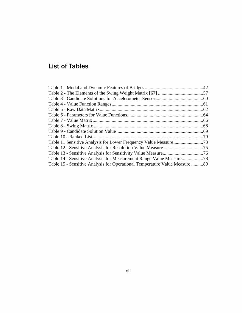
List of Tables
Table 1 - Modal and Dynamic Features of Bridges ................................................. 42 Table 2 - The Elements of the Swing Weight Matrix [67] ...................................... 57 Table 3 - Candidate Solutions for Accelerometer Sensor ........................................ 60
Table 4 - Value Function Ranges ............................................................................. 61
Table 5 - Raw Data Matrix....................................................................................... 62 Table 6 - Parameters for Value Functions................................................................ 64
Table 7 - Value Matrix ............................................................................................. 66 Table 8 - Swing Matrix ............................................................................................ 68 Table 9 - Candidate Solution Value ......................................................................... 69
Table 10 - Ranked List ............................................................................................. 70 Table 11 Sensitive Analysis for Lower Frequency Value Measure ......................... 73
Table 12 - Sensitive Analysis for Resolution Value Measure ................................. 75 Table 13 - Sensitive Analysis for Sensitivity Value Measure.................................. 76 Table 14 - Sensitive Analysis for Measurement Range Value Measure .................. 78
Table 15 - Sensitive Analysis for Operational Temperature Value Measure .......... 80

viii
Acknowledgement
A challenge makes a person innovate, create, or search for solutions. However, sometimes
we need support, method, hope, daring, and direction to stay on the right path. I had all
these, which helped me to conclude my Master’s degree course. I am blessed with all that
has happened and with who were close to me and were made part of this. Thus, I wish to
thank:
First of them was God through His Son, Jesus, who gave all I needed to be here, writing
this thesis.
My lovely wife, Adriana, who has stayed up at my side walking together on this journey,
giving me love, support, and patience. Her skills to listen and to motivate me brought me
the necessary encouragement to see beyond of the thesis process.
My advisor, Dr. Otero, the guidance in this work and for their help in reviewing the text
and the support they gave me in the completion of the course.
My colleagues, from the Brazilian Army, who strongly stimulated me to develop my skills
in Systems Engineering.
All faculties from the Department of Engineering Systems for the opportunities that you
gave me, which assuredly helped me to learn and improve professionally in field of
Systems Engineering.

ix
Dedication
I dedicate this work to all who believe that God is powerful and merciful to realize all
wishes of their hearts.

1
Chapter 1 Introduction
1.1. Research Context
Recent bridge collapses, such as the I-35W Bridge across the Mississippi River in
Minneapolis, MN, where many lives were lost, have contributed to a wide discussion
across the nation about the aging of bridges. Structural inspection techniques have been
improved over time, but with almost 600,000 bridges in the US, bridge inspectors do not
have the resources to monitor, in a timely manner, changes in the structural conditions of
these bridges. To help the inspection activities, the concept of Structural Health Monitoring
(SHM) arose, and it has improved the quality and quantity of information about the health
of bridges. Currently, there are many resources needed to use SHM systems to detect
bridge defects and to follow the aging evolution of bridge components. Methodologies,
sensors, systems, and a great deal of research have evolved to continue the improvement of
monitoring activities. This thesis presents a decision-making approach to prioritize sensors
for the development of SHM systems for bridge inspections. The resulting data are
expected to improve the effectiveness and reliability of SHM systems for bridge inspection
purposes.
1.2. Objectives
This thesis was developed to achieve three main interconnected goals. The first goal, which
was the main motivation for this research, was to identify an effective analytical
methodology to qualify and quantify vibration sensors to support decision makers in their
choice for the more adequate sensor to be employed in bridge SHM systems. To reach that
goal, the others two goals must first be meet.

2
This paper begins with a literature review of SHM, presenting it as an integrated system as
the first goal; herein are reviewed concepts, methods, and sensors related with a vibration-
based SHM environment. Next, the thesis presents its second goal, which is analyzing the
value modeling methodology, demonstrating the applicability to produce a value qualifying
and quantifying vibration sensors which can be applicable on SHM systems. Finally,
applying the research and analysis of the two previous goals, this thesis will analyze some
vibration sensors, demonstrating the applicability of the methodology, and identifying the
adequate sensors based on their specifications.
1.3. Overview of the Thesis
This thesis is organized into five. Chapter 1 provides an introduction and overall objectives
for this thesis. Chapter 2 presents results from a literature review effort, including a brief
timeline of bridge inspection evolution up to the development of SHM systems. This
chapter also presents a general definition of SHM systems, and provides descriptions of
SHM components, damage detection methods, and sensors. Chapter 3 presents the value
modeling methodology divided into qualitative and quantitative models to analyze sensor
alternatives. The objective is to support sensor-selection decisions with information that
will help to determine which sensors are better options to be used in particular SHM
systems. Chapter 4 demonstrates the practical implementation of the value-based
methodology to analyze accelerometer sensors for a particular scenario. Chapter 5 provides
concluding remarks and areas for future research.

3
Chapter 2 Review of Structural Health Monitoring of Bridges
2.1. Introduction
Transportation systems are used around the world every day by people who do not worry
about their condition because they are just system users. For society, the transportation
system should be a functional network which supports interstate trade, provides for the
daily commute of residents, and provides accessibility for relief efforts during and after
natural disasters [1].
Transportation systems are some of the most critical systems of urban infrastructure [1],
and they are composed of several critical components, including bridges[2]. Bridges are
submitted continuously to a variety of loads that stress their structure over their lifetime
[3]. Traffic flow intensity, environment, and weather conditions contribute to a progressive
deterioration at a rate which is affected by these and other factors [4].
Bridges have tended to be increasingly designed with more complex forms and functions.
By the late 1700’s, most bridges were built over canals, with stones as the main building
material. In the railroad era, locomotives demanded new technologies and materials; thus,
truss bridges, trestle bridges, and iron bridges became very popular in 1800’s. With the
mass production of automobiles in the 1900’s came the concept of reinforced concrete and
steel truss bridges, as well as concrete arches and suspension bridges [5]. Between the
1950’s and 1960’s, the nation experienced a bridge construction boom to meet the
increased demand for massive infrastructure expansions [6].
However, the bridge expansion around the nation was not matched by procedures of safety
inspections and maintenance of bridges [6]. The lack of adequate safety procedures and

4
practices led to significant failures. For example, the Tacoma Narrows Bridge, which was
opened to the public on July 16, 1940, was built with some changes to the original design
that contributed to the bridge collapsing a few months later on November 7, 1940 [5].
Another example of a major structural failure was the Silver Bridge in Point Pleasant, West
Virginia. On December 15, 1967, this bridge collapsed into the Ohio River, resulting in the
deaths of 46 people. This event marked a significant change of mind regarding the
importance of bridge inspections in the nation [6]. In 1987, New York also became part of
negative statistics when the Schoharie Creek Bridge collapsed because of scour damage,
and as result, ten people died. The scour failure turned to national attention regarding
underwater bridge inspections because approximately 86% of the over 593,000 bridges had
that condition [6]. As a result of various tragic bridge failures, the National Bridge
Inspection Program was established [7].
After various bridge collapses, bridge inspections were considered an essential activity of
bridge lifecycles. The Federal Highway Administration (FHWA) and American
Association of State Highways Officials (AASHO), developed manuals for inspectors’
training and maintenance which oriented the development of bridge inspection in the
nation. Thus, the creation of the national bridge inspection standard in the U.S. allowed the
establishment of policies regarding inspection procedures, frequency of inspections,
qualifications of personnel, reports, and bridge inventory [6]. Then, bridge inspectors and
civil engineering professionals supported by that information were able to inspect and
maintain the bridge structures by means of a manual systems of inspection, nondestructive
evaluation (NDE), and interpretation of data using conventional technologies [8].
Nevertheless, these traditional inspections methods are costly because they demand time,
qualified personnel, and specific test equipment [6] [9], which led to U.S. bridge
infrastructure to become aged and hard to monitor [8]. This highlights that bridge
inspection is a race against time, and since the bridges are constantly aging, many
structures are in poor health.
In 2003, FHWA reported 26.6% of US bridges were structurally deficient or functionally
obsolete [7], but in the last ASCE report in 2013, the numbers decreased to 24.9% of US

5
bridges which are structurally deficient or functionality obsolete. The bridge maintenance
goals over the last decade have been achieved where the states and cities have increased
their efforts, but still there is much to do [10].
The bridge deterioration phenomenon potentially increases when inadequate maintenance
occurs due fail on inspection, or repair [11]. As a consequence, tragedies involving the
collapse of bridges in the United States has happened again, and they have brought
considerable attention to the national infrastructure and have contributed to identifying its
vulnerability [1]. The I-35W bridge in Minneapolis, Minnesota, collapsed in August 2007
when the bridge was under daily loading conditions. The consequences were disruptions to
the day-to-day activities of citizens, substantial economic losses, and most important, the
loss of 27 people lives and the 200 people who were injured [1]. Such tragedies have
contributed to making SHM an important tool for bridge inspections activities [9].
Indeed, a bridge’s safety was assured only with inspections and maintenance [12], and a
proper maintenance and monitoring of the bridges were more of a national priority than
they have ever been [1], so Bridge SHM Systems began to be developed, improving the
bridges’ safety[9], providing better assessment conditions and more efficient decision-
making systems in maintenance and rehabilitation programs [1]. This is a result of
investments in new technologies and research, which has contributed to improving the
bridge inspections, and consequently, the performance of inspections and maintenance has
increased during last decades significantly. The reason for the field of SHM has grown in
last decades [13].
Thus, the recent interest in SHM highlights its high potential to improve significantly the
life-safety and economic benefits for society [8]. The adoption of SHM on transportation
systems as a bridge monitoring solution has improved the system management capability
to monitor their critical structures, such as bridges, and it is helping the transportation
system to forecast harmful events and enhance the efficiency of maintenance service of
those critical structures [12]. In this way, SHM has helped the bridge inspectors and civil
engineering professionals to optimize their manual systems of inspection procedures,
which are hard to execute and often are costly.

6
Therefore, today there is a great deal of research developing technologies, methods, and
procedures which have contributed to development of SHM, mainly in USA, Japan, Hong
Kong and Europe, with applications on highway and long span bridges especially [14]. For
example, there is much research on vibration-based method on bridge scour [15], time-
frequency methods on dams [16], fiber optic based SHM on metallic bridges [17], and
damage detection through pattern recognition [18].
SHM has been designed as a system which can be customized for a variety of purposes.
Basically, a SHM system will be composed of components with the following
functionalities: sensors, data acquisition, data transmission, data processing and analysis,
and data management [19]. Every subsystem must be researched individually, due to its
own complexity. However, in a general way, bridge SHM has been designed and applied to
monitor, provide information, and detect anomalies[20], but the problem of damage
identification is the most basic factor to be considered by a bridge SHM [21], [22]. The
system objective is identifying if, when, and where damage can occur from a normal
condition [18]. This problem leads to the goal of SHM system procedures defined by
Magalhães in [23], which is to extract features from periodically sampled dynamic
responses that can serve as indicators of the structural condition of the system under
observation.
To address this problem Rytter proposed in [24] a classification of damage identification
methods into four levels. Level 1, detection, indicates qualitatively that damage might be
present in the structure. Level 2, localization, determines the probable geometric location
of the damage. Level 3, assessment, gives information of the severity of the damage, and
the last one, Level 4, prediction, applies the information gathered on the first three levels to
predict the remaining service life of the structure. In other words, Level I will provide
information that damage is present, which will be enough for most practical applications
[25]; Level 1 to Level 3 allow the damage detection methods to solve the problem without
the dependence of other information level [22]. The last one, Level 4, it is more complex
than earlier levels because it uses the data gathered to provide information about presence,

7
location, severity, and life time resting of the structure [26], and receiving a combined
information of both global and local monitoring methods [13], [25].
The following sections of this chapter will review the basic concepts behind an SHM for a
bridge, describing basic modal properties, damage detection methodologies, SHM
components, and some of the current sensor technologies used in SHM.
2.2. Definitions of Bridge Health Monitoring
Bridge health monitoring can be understood in many different ways, according to whom is
proposing the definition, but it should be noted that SHM is not one thing: monitoring [27].
This is because the simple activity of data gathering does not constitute a SHM system, and
this is due to the fact that this system consists of has many components, including an
integrated network of sensors which generate data of the bridge. To understand better the
concepts behind SHM, following are some definitions to clarify the meaning of a SHM
system.
Xu and Li [8]offer a definition for SHM as a system which generally integrates modules as
a sensory system, a data acquisition and transmission system, a data processing and control
system, a data processing system, and a structural evaluation system. These components
are applied to acquire knowledge of the integrity of in-service structures on a continuous
basis, and the first two systems are embedded on the structures, while the other three are
habitually placed in the control center of the bridge management departments. Thus, a
SHM assumes a modular feature demanding from designers an understanding of the needs
of monitoring, characteristics of the structure, environment conditions, hardware
performance, and economic considerations.
Balageas et al. [28] show that SHM aims to give, at every moment during the life of a
structure, a diagnosis of the “state” of the constituent materials, of the different parts, and
of the full assembly of these parts constituting the structure as a whole. Doing that through
uses of integration of sensors, data transmission, computational power, process ability

8
inside the structures, and employing smart materials they assure that SHM can be
considered as a new and improved way to make a non-destructive evaluation. This concept
makes possible rethinking the design of the structure, planning the full management of the
structure itself, and considering the structure as a part of wider systems.
For Boller, [29], SHM is the integration of sensing and possibly also actuation devices to
allow the loading and damaging conditions of a structure to be recorded, analyzed,
localized, and predicted in a way that nondestructive testing (NDT) becomes an integral
part of the structure and material. His definition is based on the booming development of
sensing technology in last decades in terms of size, cost, materials, design, and
manufacturing, and taking advantage of this, of an integrated way, defines SHM for him.
Thus, SHM will be required with its sensing and assessment algorithm to monitor the loads
and the damage, merging all into a holistic process such that structural health of the bridge
can be accompanied during its whole life cycle.
Farrar and Worden [30] noted that the term SHM usually refers to the process of
implementing a damage detection strategy which involves the observation of a structure or
mechanical system over time using periodically spaced dynamic response measurements,
the extraction of damage-sensitive features from these measurements, and the statistical
analysis of these features to determine the current state of system health. This process can
be applied in aerospace, civil or mechanical engineering infrastructure, and in a long-term
SHM, the output of this process would update periodically the information regarding the
ability of the structure to continue performing its intended function in light of the
inevitable aging and degradation resulting from the operational environments.
In reference [2], Cross et al. defined, shortly, that SHM is any automated monitoring
practice that seeks to assess the condition or health of a structure. Thus, with an automated
detection system using non-visual assessment, it can access any area of the structure that is
difficult or impossible to access for inspectors, increasing safety, otherwise an inaccessible
area could have its inspection neglected in a visual inspection routine.

9
In the last definition for SHM, Wenzel [31], defines SHM as being the implementation of a
damage identification strategy to the civil engineering infrastructure. For him, damage can
be defined as changes in the material and/or geometric properties of these systems,
including changes to the boundary conditions and system connectivity, so that damage
affects the current or future performance of these systems.
In sum, SHM can be defined as a system which performs a specific function with each
integrated system component to gather, process, transmit, store, and analyze the status
from a structure where it is deployed to detect, assess, and predict the damage of that
structure.
2.3. Types of Monitoring
A structure can be monitored using multiple types of SHM systems. However, there are
two categories that should be considered to understand what kind of system will better
attend the monitoring needs. Time frame and scale of monitoring are necessary
considerations that should be addressed before choosing a type of monitoring system [9]. A
bridge infrastructure manager might want to monitor the health of an old bridge for a
period of a year or some few months, while in other cases only a one-time short-term
solution would be enough, or conversely, a new structure with an expected lifetime higher
than 40 years could have integrated a monitoring system that would last the whole
structure lifetime.
2.3.1. Time Frame
Monitoring can be executed to attend to the inspection recommended for the specific
structure, or for each life phase of the structure. It should be the most effective in
monitoring time to yield the intended results. The correct time frame is one of the factors to
be observed together; other key life phases are construction, usage, performance
evaluation, rehabilitation, and demolition [3].

10
Short-term is monitoring deployed on a bridge to obtain structural information for a short-
term objective [32].This term of measurement usually needs quality systems with lower
system performance [29].
Long-term is usually the duration of monitoring over more than one year, and it is common
with new, or retrofitted high-performance structures and structurally deficient bridges,
where public safety can be threatened in case of failure [32]. Long-term measurements
require robust sensors, high-performance components, and data acquisition systems [3].
Scheduled Inspection is a monitoring process which uses visual inspections and
nondestructive testing to assess the structural health condition of the bridge. It occurs as a
part of a regularly scheduled maintenance program with a maximum 24-month interval [1].
2.3.2. Scale
SHM has two distinct focuses on the size of monitoring coverage areas. It can aim to reach
a global or local monitoring area. Each one has specific monitoring goals which result in
monitoring, inspections procedures, and damage detection methods developed to optimize
the monitoring performance, but both are essential and important for the safe and effective
operation of bridge structures.
Global health monitoring has a basic concept of focusing on the overall health of the bridge
because when the damage occurs, it will change the stiffness, mass, or damping properties
of a structure and thus alter the global dynamic properties [9]. This method requires no
prior knowledge of the existence of damage or its location prior to deployment of the
system, so that this feature is considered advantage when it is applied to monitoring of
complex structures [13]. Global health monitoring tries to find the damage based on
changes of one or more structure modal properties as natural frequencies, mode shapes,
bridge deflection, acoustic emissions, and temperature effects[9]. When damage occurs, the
global monitoring considers that damage has an influence on the global behavior of the
whole infrastructure. Therefore, the features chosen should be sensitive to the damage [28],
having in mind that global monitoring methods are often insensitive to local initial
damage[33].

11
Once global monitoring methods have determined the potential damage locations, and if
critical areas are initially known, the extent of damage can be assessed by performing local
health monitoring methods so the damage progression may be tracked [13].
Local health monitoring methods are often used to inspect a relatively small area of a
structure because these methods tend to be time-consuming and costly [34]. Thus, local
methods are focused to find small defects on a specific location on the bridge. Application
of these methods demands calculations or experience with other structures, so that it will
possible to guess where the probable spots of damage are expected in the concerned
structure [9]. However, there are cases where the sensors and actuators cannot be
embedded in the structure, so that the area to be inspected should be accessible. This type
of limiting causes the local monitoring necessitates of specialized solutions [33], which
requires that local methods are very sensitive and able to find small defects [28]. The
diagnosis method most used in local SHM is the ultrasonic wave because it is very
sensitive to small detections due to high excitation frequencies and small wavelengths [25].
There are other numerous techniques for performing local damage detection and
assessment by magnetic fields or by radiographic, and eddy-current and thermal field
methods, for example.
2.4. Damage Detection Methodologies
The most common methodologies used for damage detection in bridge Structural Heath
Monitoring are non-destructive testing and evaluation (NDT/E) methods and vibration-
based methods [22]. The first methods apply the local monitoring concept where the
procedures require that the area of the damage is known a priori and that the inspected area
of the structure must be accessible. The second method involves the global monitoring
concept where complex structures can be monitored.
As cited before, Ritter [24] classified damage detection methods, dividing them into four
levels:

12
Level 1 (detection): indicates qualitatively that damage might be present in the structure;
Level 2 (localization): determines the probable geometric location of the damage;
Level 3 (assessment): gives information of the severity of the damage;
Level 4 (prediction): applies the information gathered on the first three levels to predict the
remaining service life of the structure.
The damage information provided by Level 1 will be enough for most of the practical
applications [25] being capable of detecting damage , but cannot provide information about
location and severity [26]. The Level 2 method will be able of providing more damage
details than the first level, adding the location of the damage, and can be obtained from
structural modal analysis such as Level 1 [35]. Level 3 allows the damage detection
methods to solve the problem without the dependence of another information level [22],
and damage information can be found coupling more than one method with a structural
model [35]. Level 4 is generally related to fracture, fatigue, and structural design analysis,
so that it is the most complex than earlier levels because it needs more data gathered to
provide an effective prediction of remaining lifetime of the structure [26].
2.4.1. Non-Destructive Testing and Evaluation Methods
Non-destructive testing and evaluation (NDT/E) methods allow inspectors and engineers to
inspect and monitor quickly and effectively bridge structures [36]. As NDT/E methods can
help prevent a premature bridge collapse, they have been researched to provide new
application guidelines, improving the damage detection activity [22]. Thus, the choice of
more suitable NDT/E methods in inspections activity is essential, as well as observing that
in some cases, more than one method is necessary to acquire a complete structural status
assessment [22].
2.4.1.1. Visual Inspection
The versatility of visual inspection makes it one of the most common methods of local
monitoring [13] and NDT/E techniques for visible areas inspection [36]. It is a powerful
inspection tool of the default bridge inspection methodology used by bridge inspectors [1].

13
However, this technique has some limitations which can impact the results of inspections
and compromise the findings. The most important factor of the visual inspections is the
human factor. The inspector’s activity performance is highly dependent on experience and
knowledge [6], particularly with structural behavior, materials and construction methods
[36]. His opinion can lead to large variations and subjectivity [1] in damage interpretation,
impacting the decision-making process [13]. Visual inspection is largely used as the first
step in concrete structures’ evaluation for monitoring the damage [36]. It is a time
consuming activity where the requirements relating to this type of inspection leads to the
closure of traffic on the bridge, though it is a quick method to identify visible and
superficial damage [36].
2.4.1.2. Ultrasonic Method
The ultrasonic inspection method has been used for bridge inspection to assess the concrete
quality[37]. A derivative method called ultrasonic pulse velocity is used to determine the
concrete strength, homogeneity, and to monitor the cracking and deterioration. The
propriety of velocity of a pulse of compressive waves through a medium that is a function
of the elastic properties and density of the medium is used as the base of this method [8].
This method utilizes high-frequency sound with a range of 25 to 100KHz [8].
2.4.1.3. Acoustic Emission Method
The acoustic emission method uses a phenomenon which occurs when a structure starts to
generate stress waves when an applied load provokes an internal pressure releasing energy
[38]. When the structure undergoes a rapid release of energy, internal cracking can appear
[22]. Thereby, a bridge structure can deform elastically, changing the stress distribution
and the storage of elastic strain in the bridge [38]. Acoustic transductors detect ultrahigh
frequency sound released by material stress. The acoustic emission method has been used
monitoring cracking, crack development, and corrosion [22]. A feature of this method
allows structural damage assessment detecting and locating flaws, but it cannot determine
the size of flaws [22].

14
2.4.2. Vibration Based Methods
Second Magalhães [23], basically the goal of all vibration-based SHM is to extract features
from periodically sampled dynamic responses that can serve as indicators of the structural
condition of the system under observation. Thus, vibration-based SHM damage detection
methods rely on changes in global vibration parameters [34] provoked by damages in
bridge structures [39]. These dynamic features measured are mainly modal parameters
[40], and the evaluation of changes in those physical properties can hence be used to detect
structural damage or degradation [20], [39].
Structural modal parameters are identified through modal analysis techniques that gather
data based on input-only, input-output, and output-only measurement. Under operational
conditions, and not under a test condition with controlled vibration source, in the input-
only and input-output measurements, it is extremely difficult to quantify the input forces or
external excitation [19]. On the other hand, in the output-only measurement, it is easy to
measure the output data, allowing the identification of the structure modal parameters[23].
An output-only measurement does not use external equipment to excite the bridge
structure, and the bridge does not have to be closed in order to execute this measurement
technique [19].
Applying output-only modal analysis to identify the bridge structure modal parameters will
be possible, estimating the most common structural vibration characteristics as natural
frequencies, mode shapes, and modal damping ratios[23], but also the flexibility directly
derived from the unit-normal modal vectors [19]. For example, when damage reduces the
stiffness of the structure, it changes its vibration characteristics [34]. Therefore, changes
measured in the modal parameters of a structure can be used to detect, locate, and quantify
the structural damage.
However, Bisby [26] related that the global vibration characteristics of large structures,
such as bridges, are only very slightly affected by local damages. In consequence, a
vibration-based SHM will necessitate a very precise knowledge of vibration characteristics
of the structure. Precise and repeated measurements to reduce the influence of variability

15
caused by random errors (including noise), and sufficient number and placement of sensors
are tasks which should be considered to optimize the SHM performances [25].
To extract modal parameters data from output-only modal analysis there are several
algorithms which can be applied to identify them, and finite elements and stochastic
subspace identification are examples of that. Finite element (FE) is a well-known
extraction function applied to the raw data [25]. Stochastic subspace identification (SSI) is
an advanced method that identifies the state space matrices based on measurements using
robust mathematical tools and uses numerical techniques, such as QR-factorization,
singular value decomposition and least squares [19].
In the process of obtaining the modal parameters by identifying precisely the bridge
vibration characteristics, it is necessary to take into consideration that the bridges are
subjected to different ambient and operating conditions [19]. Factors such as traffic,
temperature, humidity, and wind occurring daily and seasonally contribute to causing
change in modal parameters during the data gathering which can make it difficult to detect
real structural damage [20]. To deal with those environmental factors’ effects, several
researchers are developing methods to filter them from the final data [19].
Depending of the SHM design and dynamic parameters to be monitored, damage detection
methods can be categorized into time domain, frequency domain, and time-frequency
domain methods. However, most of the vibration-based methods use the frequency domain
principle [22], such as frequency response function (FRF), natural frequency, damping,
mode shape, mode shape curvature, modal flexibility, and modal strain energy, which will
be described in the following sections.
2.4.2.1. Resonant Frequency
Resonance frequency is one of modal parameters of a bridge structure, and its
measurement and monitoring offers an interesting advantage relative to other damage
detection methods, but it also has limitations. As each structure has its own range of
resonance frequencies, which are a function of mass, stiffness, and damping of the

16
structure [30], damage can be detected monitoring the occurrence of shifts in resonance
frequencies values.
The main advantages of use of resonance frequencies as a method to detect damage are that
shift frequencies can be measured deploying few sensors, and measurement results are
relatively more precise than other modal parameters measurement [22]. Hence, the
resonance frequencies can be assessed with less variability, and used as a more sensitive
damage indicator [30]. However, resonance frequencies do not carry any information about
location and severity of the damage [22], making then typically a Level 1 damage detection
method [40].
On the other hand, there are weaknesses in the resonance frequency method. Sensitivity of
frequency of damage is relatively low, which means frequency shifts caused by damage are
small compared to changes with others modal parameters [30], so that frequency
information alone cannot provide reliable results [40]. Thus, for damage in the structure to
be detected, it must be significant. A solution is to design a very precise monitoring system
able to detect minor frequency shifts, but it brings others problems, such as influence of
environmental and operational factors over resonance frequency shift and in damage
caused by them. In consequence, vibration-based SHM that uses resonance frequency
method should implement additional damage analysis techniques to locate and assess the
severity of damages to be more efficient [13].
2.4.2.2. Mode Shape Changes
Mode shapes are modal properties of structures, and can be used as information on the
damage detection process in SHM analysis [3]. Mode shapes are represented by a set of
orthogonal vectors, and are defined by a modal model that span the system’s dynamic
response space [30]. Each bridge structure has specifics mode of vibrations, and
consequently, each one has associated mode shapes. These modal properties, as resonance
frequencies, also are a function of mass, stiffness, and damping of the structure, so that
mode shapes are affected by occurrence of damage in these parameters [13].

17
Mode shapes are spatially defined quantities, and thus they are able to provide more
complete damage information than resonance frequencies showing the occurrence and
location of the damage [40]. That property is considered the most advantageous of mode
shape methods over resonance frequency method for damage detection [13]. Also, modal
shapes often reflect the distribution pattern of the damage when modal vibrations are the
reason for the damage occurrence [3].
Mode shapes have limitations similar to the resonance frequencies method. A considerable
number of sensors monitoring the structure is required to be distributed in many locations
of the structure. This is needed to determine with high accuracy the mode shapes, and any
changes caused by damage due to mode shape monitoring methods, such as resonance
frequencies, have low sensitivity to damages [13]. When the bridge structure is excited at
low frequencies the sensitivity problem of the modal shapes method becomes more
evidenced; meanwhile, at high frequencies the respective mode shapes are more sensitive
than resonance frequencies to detect damage in structures, but high frequency modes of
excitation are not usual in an operational day and are difficult to induce [13]. Thus,
vibration-based SHM which is using mode shapes measures bridges’ mode shapes directly,
or mode shapes properties, such as curvature or modal strain energy, to improve sensitivity
of the damage detection and location [40]. However, it is common to employ mode shapes
as a source of statistical features feeding other more decisive results in activities of damage
detection, location, and estimation of severity [3].
2.4.2.3. Dynamic Flexibility Matrix
Being the inverse of the static stiffness matrix, the flexibility matrix relates dynamic values
of the structure, such as the applied static force and resulting structural displacement. The
flexibility matrix can be employed in a vibration-based SHM, measuring dynamically the
bridge structure to estimate changes in the static behavior of the bridge. The flexibility
matrix is formulated through calculus, based on the mass normalized, mode shapes and
frequencies, and normally it only considers the first modes at lowest frequency modes of
the structure measured. However, a complete static flexibility matrix requires the
measurement of all mode shapes and frequencies of the structure [35].

18
The columns of the flexibility matrix of the bridge structure represent the displacement
pattern for a specific degree of freedom related with applied force in the structure. So, by
analyzing the degree of freedom it will be possible identify the location of damage; hence,
it will be indicated by the maximum variation in flexibility from the undamaged state
represented among the DOF. This variation in flexibility is made by comparing the
flexibility matrices synthetized using modes of the damaged structure with the flexibility
matrix synthesized using modes of the undamaged structure or the flexibility matrix from a
FEM [35]. The main benefit of this method is that the flexibility matrix is more sensitive to
changes in the lower-frequencies modes [35], and it is due to its property to be inversely
related to the modal frequencies.
2.4.3. Pattern Recognition Methods
A vibration-based SHM can be subject to subtle signal data changes provoked by dynamic
structural behavior due to the occurrence of the damage [3]. Signal changes can be difficult
to interpret using traditional modal properties analysis. Because damage detection is the
most basic question to be answered in SHM [21], there are situations where automated
pattern recognition methods may improve damage detection and location [3]. These
methods are a field of artificial intelligence which uses machine learning techniques and
algorithms to detect damage in bridge structures [41].
Depending on the time frame of the SHM deployed on the bridge, the speed of data flow,
their sheer volume, and diversity highlight the limitation of human natural capability to
analyze the data yielded in real time [42]. Hence, due to the complexity of extracting
information from data of vibration-based SHM system, some pattern recognition methods
are being employed to soften that problem. These methods are characterized by assigning
of some sort of output values to a given input value, and they are implemented according to
some specific machine learning algorithms.
Machine learning is an artificial intelligence implemented by software which has the
capability to optimize a specific set of performance criterion. It is made through analysis of
data or past experience examples applying its learning capability techniques [43]. Thus,
machine learning can help the structural damage detection because it is able to identify,

19
locate, and estimate damage severity, creating a predictive model to make predictions using
the knowledge base from data. Whereas the SHM can provide a detailed model where there
are measured parameters, which can be used to create a pool of data to be processed and
analyzed, the machine learning will be highly useful. It is able to process and combine a
great deal of complex data streamed, and it has as objective to extract intrinsic patterns and
develop predictive models [18]. Machine learning techniques are applied in SHM damage
detection using inductive learning, or learning by examples of algorithms [40]. The most
common algorithms used for the characterization of bridge structural damage in vibration-
based SHM are artificial neural networks, genetic algorithm, and fuzzy logic [18].
2.5. Structural Health Monitoring Components
A bridge SHM must be designed accordingly with monitoring objectives, and considering
that each bridge has specifics characteristics and unique demands. An appropriate SHM
will be capable of helping the bridge managers to determine the ability of the structure to
provide adequate service, and to assess the necessities of maintenance, repair, or
replacement of the parts or whole bridge structure.
Considering the scope of the SHM, it will demand a detailed and complex system which
must be capable to provide information from the health of bridge structure to any
significant damage that has been detected. Thus, a SHM should be designed considering
some monitoring aspects, such as the kind of parameters to be monitored, the parameters’
properties, the processing data capability, the environment of monitoring, the duration of
monitoring, and others.
Involving all these aspects into a package solution will result in a complex SHM system
which can be divided into components. Today the SHM systems consist of five common
components while the details of whole system can vary according to the monitoring
necessities. Thus, the components can be divided into the following:

20
1. Sensory system;
2. Data acquisition system;
3. Data transmission system;
4. Data processing and analysis system;
5. Data management system.
Hence, to build an appropriate comprehension of the structure and elements of a bridge
SHM system, presented below is an introduction to SHM components.
2.5.1. Sensory System
The sensory system has the responsibility to sense changes (e.g., displacement) to
structural components. This system is composed of many sensors distributed along of a
bridge to gather signals of interest yielded around and into the bridge [8]. Thus, the number
of sensors should be determined to attend to the size and complexity of the bridge structure
according to the monitoring objectives.
Signals yielded by sensors are collections of raw data such as strains, deformations,
accelerations, temperatures, moisture levels, acoustic emissions, and loads. Various types
of sensors may be used to collect these data and may include: load cells, electrical
resistance strain gauges, vibrating wire strain gauges, displacement transducers,
accelerometers, anemometers, thermocouples, and fiber optic sensors [19], [26]
However, the sensors should be carefully selected such that their performance can meet the
monitoring needs [8]. Thus, sensors have some major performance features that must be
considered, such as measurement range, sampling rate, sensitivity, resolution, linearity,
stability, accuracy, repeatability, frequency response, durability. In addition, sensors must
be able to deal with environment constraints such as temperature range, humidity range,
size, packing, isolation, and thermal effect [44].

21
2.5.2. Data Acquisition System
The data acquisition system (DAS) is the intermediate component onsite of the SHM
system, that it is localized between the sensors and computers, responsible by data
processing. The DAS is responsible for collecting signals generated by the sensors,
converting the signals, and delivering them to the transmission system to be transmitted to
the processing data component [8]. The DAS is composed of hardware, software, and
secondary equipment such as connectors, cables, and cabinets [45]. This DAS modularity
feature facilitates the design of specific SHM solutions, allowing a customized system
adapted to monitoring needs.
The DAS converts the electrical signal generated by sensors distributed along the bridge
structure in digital data executing preprocessing and local buffering [45]. The signal is
transferred to the DAS, being gathered directly from sensors by cable or wireless
transceivers. Cables are the most common communication choice, but very long cables can
lead to errors resulting from electromagnetic interference (EMI), particularly in the
presence of high-voltage power lines or radio transmitters [26]; also, there are problems
with cost and installation time which often limits their uses in some cases [46]. Wireless
transceivers are being used as a solution to optimize the sensor distribution on building
structures, allowing a faster and cheaper installation in some cases, but there are still
problems such as limitations of the number of sensors, a low sample rate [46], and power
consumption in long monitoring activities [30].
Regarding system performance, the DAS should implement solutions to deal with many
possible sources of error and uncertainty about data gathered from sensors installed in the
bridge structure. The cause of this concern is that likely the data contains extraneous
information and noise that are not applicable for the purposes of SHM activity [19].
2.5.3. Data Transmission System
The data transmission system (DTS) is the SHM component used to transfer the data
gathered by DAS from the sensors to the location where they will be processed and
analyzed [8]. The DTS transfers the data from the remote location where the DAS is
22
installed to a processing center located a few miles away. This feature of DTS is important
for the SHM system because it allows that bridge to be monitored remotely from the
operation center, so that the constant visits or inspections by inspectors and engineers can
be eliminated or reduced.
The DTS requires physical transmission media, physical transmission mechanisms, data
modulation techniques, and data interface protocols [3]. SHM systems employ a variety of
custom communication link technologies and network protocol. For communication links,
the most common solution is to use fiber optics cable, single modes for shorter links and
multi-mode fibers for links higher 600 meters, wireless technologies such as radio or
cellular transmission, and telephone lines, or hybrid systems [26]. In the case of network
protocols, the most commons protocols available are employed such as Ethernet, RS-232,
RS-485, and IEEE-802.11 protocols family [8]. However, DTS is still a field that continues
to increase in diversity of architectures and transmission capability, searching for
improvements in performance, optimization of bandwidth, and energy consumption [3].
2.5.4. Data Processing and Analysis System
The data processing and analysis system (DPAS) is the SHM component responsible for
processing collected and preprocessed raw data from sensors and DAS, and converting
these data into valuable structural health information. Thus, the DPAS encompasses a
complex multistage and multiscale process which uses extensively data processing and
statistical analysis techniques to make prognoses about bridge health status [3].
The volume and complexity of transmitted data from sensors and DAS tend to increase
with the SHM system size. Handling a huge number of data, extracting bridge health
information, and analyzing the processed data are critical activities of the DPAS [8]. There
are many processing techniques which can be used on DPAS to perform these activities
DPAS and to yield an effective structural condition evaluation on the SHM system. Data
fusion and data mining are examples of processing techniques used on DPAS.
Data fusion is a process used to integrate the data from various types of SHM sensors
deployed on the bridge. This integration process aims to produce improved information, to

23
be used as single information alone. Data fusion can be categorized in low, intermediate,
and high levels, based on what stage of the process fusion occurs. In the low level fusion
there is the combination of raw data from sensors yielding new data which is more
informative and compact than former sensor data. The intermediate level fusion extracts
features from raw data and combines them into a concatenated feature vector. In the high
level fusion decisions, which comes from decision systems, they are combined to reach a
consistent conclusion [8].
Data mining is a process which uses a nontrivial algorithm to identify valid, novel,
potentially useful, and ultimately understandable patterns in the database. This makes data
mining a bridge between the data and extracted features for the decision making process.
Regression analysis, clustering analysis, and principal component analysis are the most
conventional statistical data mining methods [8]. Support vector machines, genetic
algorithms, and artificial neural networks are the most used machine learning methods for
data mining [3] applied to bridge structural damage detection.
2.5.5. Data Management System
Data management system (DMS) is the SHM component which comprises the database
system for temporal and spatial data management yielded on bridge monitoring [8]. The
data gathered, transmitted, and processed by other SHM components should be stored and
managed properly for display, query, and further analysis. Also, relevant information about
the bridge structure, such as computational models, design details, and others related with
SHM activities must be documented and stored as well [3].
The DMS may implement the data management strategy using the several available
architectures and technologies to attend the SHM systems’ demands. Rules to eliminate
unnecessary data, to record data changes, to classify data, and how long data should be
stored are types of data management strategies to be developed. In addition, the DTS
should develop algorithms to assure the data quality in activities of processing, storing, and
retrieving [19], so that a reliable database can be created, staying viable for many years
with a low susceptibility of being corrupted.

24
2.6. Sensors Used in Structural Health Monitoring
Sensors used to collect the data from bridge structures and the environment should attend
to the technical requirements defined for the SHM system to perform the monitoring needs.
The sensors of the bridge SHM system are generally applied for monitoring loads on the
structure, the structural responses, and environmental conditions[8]. Normally, the sensors
used on SHM are inexpensive, durable, easy to install and maintain, and can output
information directly regarding the health status of the structure [47].
This section provides an overview of the most common sensor types which are employed
and researched in SHM systems to measure the bridge behavior under external excitation.
The sensors are organized by their operating mechanisms which are mechanical, electrical,
electromagnetic, optical, modern physics, and/or chemical effects.
2.6.1. Accelerometers
Accelerometers are devices widely used to measure the acceleration of structures due to
displacements or vibrations induced by external excitation. The acceleration measurement
is made from a particular point of the structure where the accelerometer is mounted [47]. In
the case of bridges, the acceleration responses are closely related to serviceability and
functionality of the bridge [8]. The data provided by accelerometers will be used to obtain
dynamic characteristics of the global structure such as natural frequencies, damping ratios,
and mode shapes [8]. These characteristics are directly related with the mass, stiffness, and
damping of the structure.
Accelerometers are developed based on the mechanical concept of the system made up of a
damped mass on a spring [47]. Upon an external excitation, the mass is constrained to
move on a given axis, and this mass displacement makes the spring accelerate
proportionally to the actual acceleration of the structure [48]. The measurement result is
obtained from a numerical integration of the data, but in the integration process there are
errors that may be reduced, adjusting and improving the time variation of displacements
[3]. However, the accelerometers still are the best sensors available to measure dynamic
properties of the bridge structures.

25
2.6.1.1. Piezoelectric Accelerometers
The piezoelectric accelerometer is the most popular accelerometer of this type of sensor. It
is composed basically of three elements which are a piezoelectric element attached in a
seismic mass that is coupled to a structural base [19]. Its main sensing element is a piece of
piezoelectric material, which is a material able to self-generate an electric signal
proportional to external excitations when submitted to them, and without the necessity to
receive any input electrical or power source [44]. Thus, when the structural base of the
piezoelectric accelerometer is submitted to a vibrational movement, the mass exerts an
inertial force on the piezoelectric crystal which will produce an electric charge [8]. Thus,
the output will be an electric signal proportional to the acceleration caused by vibration
movements of the bridge where the sensor is mounted, and that will be received by DAS
into SHM context.
Figure 1 - Basic piezoelectric accelerometer construction [49]
The piezoelectric accelerometers are very useful for SHM application because they are
durable, easy to install, and have a large dynamic range, stability and long life span [8].
This type of accelerometer has the characteristic of being able to operate at low and high
temperatures, up to 350oF [49], and it has high reliability operating over a fairly wide
frequency and amplitude range [44]. However, there are relevant drawbacks on
piezoelectric accelerometers. They cannot measure very low frequency, around 0.1Hz, [3]
because they are not sensitive to true DC levels [8], so that this type of sensor is not
indicate to measure vibrations of large structures [3].

26
2.6.1.2. Capacitive Accelerometers
Capacitive accelerometers are sensor devices which utilize an opposed plate capacitor to
sense a capacitive shift created by the influence of displacements and vibrations measuring
the acceleration across the bridge [44]. The capacitive sensing element consists of two
crystal silicon’s electrostatically bonded, forming parallel plate capacitors acting in a
differential mode [49]. Operating in a half bridge configuration, the capacitors are
dependent on a carrier demodulator circuit or its equivalent to produce an electrical output
proportional to acceleration [49]. Capacitive type accelerometers are very accurate and
have excellent measurement resolution for a wide range of vibration levels, from micro g
(gravity acceleration = 9.80 m/s2) to 100s of g through a frequency range from DC to very
high frequencies [44].
Figure 2 - Capacitive sensor element construction [49]
The result is a sensor which provides a response to DC acceleration inputs with stable
damping characteristics that maximize frequency response, so that making it an
accelerometer highly adequate for civil flexible structures, they can measure accelerations
from DC level [8], and present ruggedness to withstand extremely high acceleration over-
range conditions [44].
2.6.1.3. Piezoresistive Accelerometer
Piezoresistive accelerometers are sensors which use a piezoresistive strain gauge as a base
to measure the acceleration of the structures. The sensitive material is made of a solid state
silicon resistor which changes its electrical resistance proportionally to the force or stress

27
applied on it [49]. These accelerometers are designed with discrete strain gauges
mechanically attached to a cantilever beam with a seismic mass attached.
Figure 3 - Schematics of piezoresistive accelerometer [44]
The acceleration is measured through an output electric signal produced by a Wheatstone
bridge circuit connected to piezoresistive strain gauges [44]. When the sensor suffers
acceleration, the seismic mass stresses the strain gauges flexing it, which alters the
electrical signal output proportionally to vibratory motion. The advantage of this type of
accelerometer is that the piezoresistive element provides very low frequency response;
thus, it is possible to measure accelerations down to 0 Hz and from DC levels, which
cannot be achieved with piezoelectric materials [50]. On the other hand, the main
drawback is that it requires constant electrical input for the Wheatstone bridge circuit, and
it has a small dynamic range of measurement [44].
2.6.1.4. Servo Accelerometer
Servo accelerometers are sensors with a close-loop design [49]. They have low-frequency
sensitivity due to the soft spring and an electromechanical servomechanism [3]. They were
designed to keep internal deflection of the seismic mass to an extreme minimum to reduce
the errors due to nonlinearities of the mass flexure, but the mass displacement presents a
finite error which is intrinsic to piezoelectric, piezoresistive, or variable capacitance
accelerometers [49]. So, in servo accelerometers the mass is maintained in a “balanced”
mode, virtually contributing to eliminate errors due to nonlinearities.
28
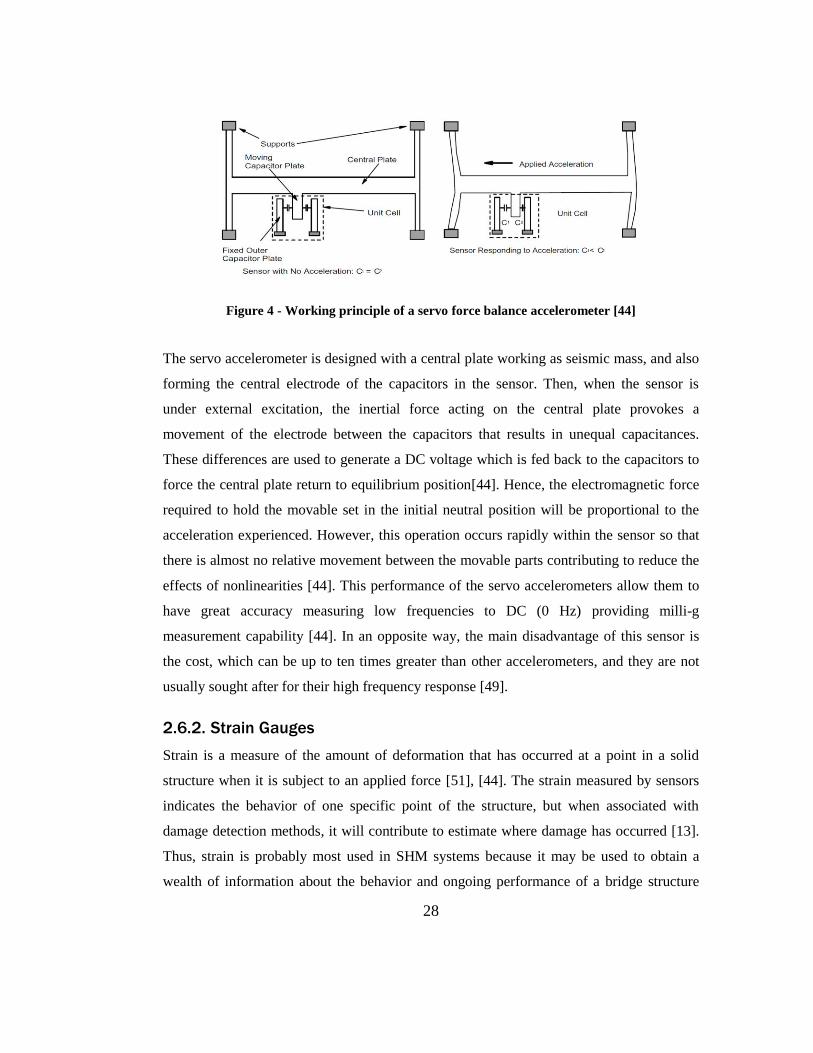
Figure 4 - Working principle of a servo force balance accelerometer [44]
The servo accelerometer is designed with a central plate working as seismic mass, and also
forming the central electrode of the capacitors in the sensor. Then, when the sensor is
under external excitation, the inertial force acting on the central plate provokes a
movement of the electrode between the capacitors that results in unequal capacitances.
These differences are used to generate a DC voltage which is fed back to the capacitors to
force the central plate return to equilibrium position[44]. Hence, the electromagnetic force
required to hold the movable set in the initial neutral position will be proportional to the
acceleration experienced. However, this operation occurs rapidly within the sensor so that
there is almost no relative movement between the movable parts contributing to reduce the
effects of nonlinearities [44]. This performance of the servo accelerometers allow them to
have great accuracy measuring low frequencies to DC (0 Hz) providing milli-g
measurement capability [44]. In an opposite way, the main disadvantage of this sensor is
the cost, which can be up to ten times greater than other accelerometers, and they are not
usually sought after for their high frequency response [49].
2.6.2. Strain Gauges
Strain is a measure of the amount of deformation that has occurred at a point in a solid
structure when it is subject to an applied force [51], [44]. The strain measured by sensors
indicates the behavior of one specific point of the structure, but when associated with
damage detection methods, it will contribute to estimate where damage has occurred [13].
Thus, strain is probably most used in SHM systems because it may be used to obtain a
wealth of information about the behavior and ongoing performance of a bridge structure

29
[26]. The most common types of sensors used to measure it on bridge monitoring are
resistance foil strain gauges, vibrating strain gauges, and fiber optic strain gauges [19].
2.6.2.1. Electrical Resistance Strain Gauges
Electrical resistance strain gauges are sensors in which the operating principle is based on
the principle that the resistance of a conductor will change in direct proportion to a change
in its length [44]. When the conductor wire is stretched, the conductivity increases and
when it is compressed, the conductivity decreases; this phenomenon is known as the
piezoresistive effect [51]. The electrical resistance strain gauge is the most widely used
strain gauge sensor, and the bonded foil resistance strain gauge is one of the more used,
being most suitable for short monitoring duration [44], and less attractive for applications
when the distance between the gauge and the readout unit increases [19].
Figure 5 - Bonded foil resistance strain gage [44]
The bonded foil resistance strain gauges are made of a thin metallic film deposited on a
nonconducting plastic film. They are attached to the structure basically in three different
ways: bonded, weldable, and embedment. The first attachment mode is the most indicated
when the highest accuracy is desired. The second mode is indicated for situations where
the bonded are not ideal, and the third option is indicated to measure strains inside of
concrete structures [19]. These sensors require a constant external power source for
excitation, and they can have problems with self-heating, which can cause them to drift
[44]. Thus, to lead with them, a higher resistance gauge is preferentially used because it is
less susceptible to self-heating effects and to lead wire effects [44].
30
2.6.2.2. Vibrating Wire Strain Gauges
Vibrating wire gauges are well-stablished sensors in bridge monitoring applications due to
their long-term performance and reliability [44]. Vibrating wire strain gauges are
commonly used to measure incremental strains due to temperature changes, soil pressure
changes at the abutments, and temperature differentials of the bridge [44]. These gauges
consist of a thin steel wire held in tension between two end anchorages [8] being mounted
on the bridge structure at two points [3]. The wire will vibrate due to structural strain
caused by an external excitation, which will promote a relative displacement of the
anchorages and stretch of the wire [3]. Vibration frequencies are measured based on
changes in the tensioned wires due to the distance changes between the anchorages [8],
[44]. This measurement method is very stable and the results are very reliable, so that it
may be applied on structures monitored continuously for long periods of time without any
zero drift [44].
However, vibrating wire strain gauges are most suitable for measuring static or slowly
varying strains[44], and the strain measured can be transmitted over a higher distance than
foil resistance strain gauges without much degradation [8]. The main drawbacks of
vibrating wire gauges are that the gauges tend to be fairly large, require bulky cables, and
can measure the static strain only, as it takes seconds to obtain the frequency of the
vibrating wire [3], [8].
2.6.2.3. Fiber Optic Strain Gauges
Fiber optic strain gauges are sensors which have characteristics that make them useful
sensor options for bridge monitoring applications, such as fast response, immunity to
EMI/RFI noise sources and lighting, low attenuation of the sensor signal, multiplex
capability, and they are suitable for both static and dynamic measurements [8], [44], [22].
On the other hand, the major drawback of fiber optic strain gauge sensors is the high cost
of sensors and their associated signal conditioning. The fragility of the fiber demands that
the sensors must be handled carefully during the installation process [22], [44]. Fiber optic
strain gauges are available in various different forms, but they are commonly available in

31
of two basic forms, fiber optic Bragg gratings and Fabry-Perot interferometric (FPI) gauges
[26].
Fiber Bragg grating (FBG) sensors are commonly used to measure the strain in bridge
monitoring applications. This sensor has optical gratings etched directly onto the fiber [44],
and the grating spacing is proportional to the wavelength of light reflected in the fiber [26].
Consequently, the strain measurement principle is that the variations on structure strain
will cause shifts in the wavelength of the light [8]. FBG sensors are able to measure local
point strains only, and they can be used for both static and dynamic monitoring, and can be
serially multiplexed [26]. This feature allows one optical fiber to accommodate six to ten
FBG sensors [8]. Nevertheless, the main disadvantages of FBG for strain measurements
are that it requires DAS components more expensive than conventional strain gages, it is
less accurate than EFPI sensors, and it must use a reference grating for temperature
corrections[44].
Figure 6 - Operating principle of fiber optic Bragg grating [3]
The Fabry-Perot interferometric gauge (FPIG) consists of fiber optic cables in which the
optical fiber is cut and a gap is inserted between the two ends of the severed fiber. The
sensing element of the FPIG is external to the optical fiber, and it consists of two mirrors
which face each other and are separated by an air gap or cavity [44]. This sophisticated
optical technique is used to extract the strain through the measurement of the wavelengths
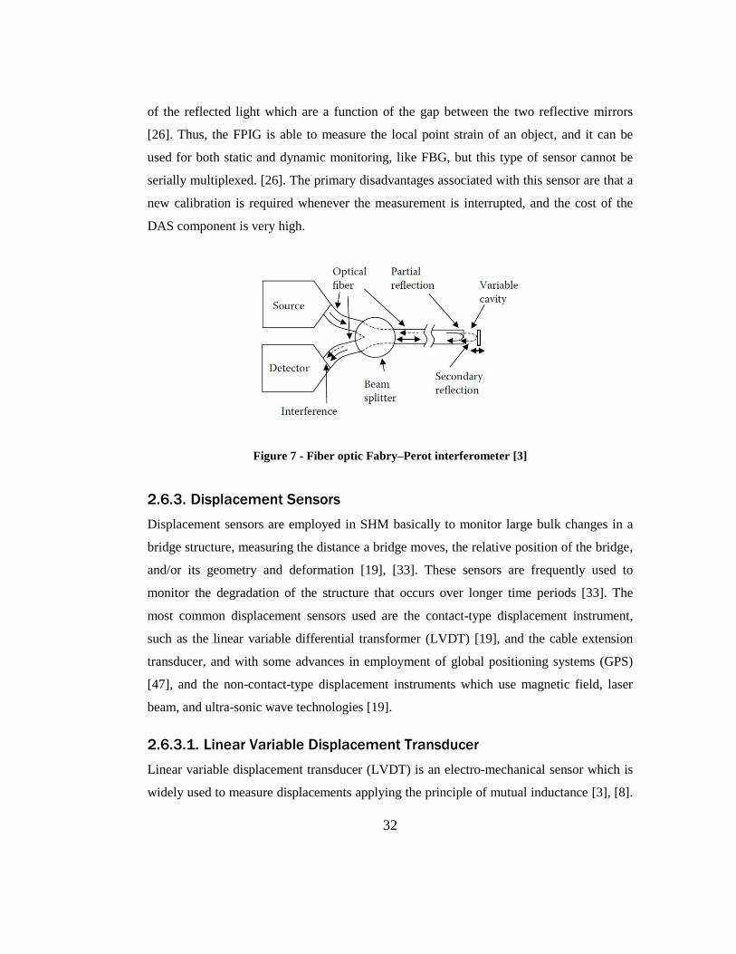
32
of the reflected light which are a function of the gap between the two reflective mirrors
[26]. Thus, the FPIG is able to measure the local point strain of an object, and it can be
used for both static and dynamic monitoring, like FBG, but this type of sensor cannot be
serially multiplexed. [26]. The primary disadvantages associated with this sensor are that a
new calibration is required whenever the measurement is interrupted, and the cost of the
DAS component is very high.
Figure 7 - Fiber optic Fabry–Perot interferometer [3]
2.6.3. Displacement Sensors
Displacement sensors are employed in SHM basically to monitor large bulk changes in a
bridge structure, measuring the distance a bridge moves, the relative position of the bridge,
and/or its geometry and deformation [19], [33]. These sensors are frequently used to
monitor the degradation of the structure that occurs over longer time periods [33]. The
most common displacement sensors used are the contact-type displacement instrument,
such as the linear variable differential transformer (LVDT) [19], and the cable extension
transducer, and with some advances in employment of global positioning systems (GPS)
[47], and the non-contact-type displacement instruments which use magnetic field, laser
beam, and ultra-sonic wave technologies [19].
2.6.3.1. Linear Variable Displacement Transducer
Linear variable displacement transducer (LVDT) is an electro-mechanical sensor which is
widely used to measure displacements applying the principle of mutual inductance [3], [8].

33
The LVDT is also well known as a linear variable differential transformer [47]. This sensor
uses a type of electrical transformer, with three coils being the central the primary coil, and
a movable magnetic core to measure linear displacement [3]. Applying an AC excitation to
the primary coil, it will generate a proportional inductance current on secondary coils.
Whether the core is equidistant to both secondary coils, no voltage will appear at the
secondary coils’ output. However, whether the core moves, a differential voltage will be
induced at the output [19]. Hence, the coils will produce an output voltage that will be
proportional to the position of the moving core [8], providing the displacement of the
monitored point through a piston-like motion of core inside of the transformer [3].
Figure 8 - Schematic of LVDT [3]
This displacement sensor is very accurate due to the frictionless movement of the core,
which contributes to a very long mechanical life, very high resolution results suitable for
use in very low temperatures, and long-term stability [8], [19]. Nevertheless, LVDT
displacement sensors can be costly due to the necessity of being attached to the structure,
making them impractical applications in large structures [47], but at same time, they are
applicable in many situations where linear potentiometers cannot be utilized [13].

34
2.6.3.2. Cable extension transducer
A cable extension transducer is a sensor device usually employed to measure linear
displacements [44]. Consisting basically of a spool, a tension spring, and a precision linear
potentiometer, this instrument also utilizes a flexible stainless cable wound on the spool
tensioned by a spring that keeps the cable loaded [52], [44]. So, using the radius of the
spool, which is known, together with the measurement of its rotation, it is possible to
calculate the displacement of the point monitored [53]. Mounting the sensor to a fixed
reference and attaching the end of the steel cable onto the structure component which
displacement is being measured, when the cable is extended or retracted, the linear
potentiometer will measure the displacement by movement of the steel cable wound on the
spool [53]. The potentiometer uses the principle of variable resistance to measure
displacement, and its wiper moves toward one end of the resistor, changing the resistance
such that it will be proportional to the distance moved by the cable, and the output will
change with any movement of the wiper [44].
Figure 9 - Schematic of cable extension transducer and linear potentiometer [44]
The advantages of cable extension transducers are that they have a larger measurement
range than LVDTs [44], and they are suitable to measure large displacements [52]. The
potentiometer requires a voltage source to measure the changes in resistance; nevertheless,
the output signal produced by the cable extension transducer is linearly proportional to the
displacement of the extension cable, easily measured by the DAS [44]. The drawbacks of
the cable extension transducer are that their accuracy is lower [53], and they are a contact
device; hence, their potentiometers are subject to damage due to wear if the cable is pulled
35
beyond its design range. The sensor cannot be used for dynamic measurements [44], and it
is limited to low frequency vibrations[40].
2.6.4. Tiltmeters
Inclinometers, also known as tiltmeters, are sensors which measure changes in bridge
structure slope [54]. Based on vibration wire, capacitance, and inertial movement, these
instruments are used to monitor behavior of a specific point on a bridge [53] in response to
external excitations, such as temperature changes and loading conditions [9]. Being often
employed as permanent sensor in SHM application [44], the integration of slope along the
span of the bridge can be used to figure out the displacement of the structure [9]. The most
common types of tiltmeters used in SHM are vibrating wire tiltmeters, electrolytic
tiltmeters, and inertial based inclinometers. [44]. The data output gathered from tiltmeters
can be integrated with the GPS data to provide a global displacement of the bridge [8]
because knowing the slope at one point of the bridge will likely not allowthe
determination of what is happening to the structure [9]. One drawback of tiltmeters are that
they use acceleration of gravity to activate the sensing element of the transducer, so that
they are also sensitive to other forms of acceleration [3].
2.6.4.1. Vibrating Wire Tiltmeter
Vibrating wire tiltmeters are based on the principle of operation of the vibrating wire strain
gauges, but are applied to measure the tilt of the structures. They are designed to perform
long-term measurements with a pendulous mass being supported by a vibrating wire strain
gauge. When the structure experience and displacement, the mass will rotate around the
wire gauge, shifting its frequency, so that the rotation angle will calculated based on that
shift. Resistant to water and corrosion, the vibrating wire tiltmeters are not suitable for
measuring dynamic changes [44].
2.6.4.2. Electrolytic Tiltmeters
An electrolytic tiltmeter is an instrument that uses hard-anodized aluminum electrodes as a
base for its sensing element. These electrodes are part of the high-precision electrolytic tilt
transducer which also has a plastic dome and internal electronics, providing good

36
resolution and stability. The electrodes are submerged in conductive fluid inside of a small
chamber, and when the electrolytic transducer tilts, they are covered or uncovered. Hence,
it yields changes in the electrical resistance to the excitation signal which converts to
angular movement measure. The main advantage of this tiltmeter is its angular movement
of measurement does not need an external datum because it is referenced on a vertical
gravity vector. The main drawback is that this sensor is in not suitable for measuring
rapidly varying tilts [44].
2.6.4.3. Inertial Based Inclinometers
Inertial based inclinometers are most applicable in the monitoring of structures subject to
high levels of shock and vibration, such as those which may be due to traffic. Using a close
loop technology like as a servo accelerometer, these instruments have as a sensing element
a torque mechanism where the tilt is measured through angular motion readout by an
optical detector. This operating principle makes them suitable for measuring rapid changes
of slope as small as 0.1 seconds of a degree, due to live loads or dynamic events [44].
2.6.5. Micro-electro-mechanical systems (MEMS) Sensors
Micro-electro-mechanical-systems (MEMS) are very small devices, structures ranging in
size from a micrometer to a millimeter, combining electrical and mechanical functionalities
and components in one hybrid device [55], [38]. The advance of MEMS development has
allowed the emergence of many novel sensors using that technology [55], and making
them one of the principal emerging sensing technologies for the measurement of dynamic
response in SHM systems [30]. The automotive industry, with its huge production, has
facilitated to push MEMS costs down, such that it has contributed to make them available
for SHM applications. Hence, sensors based on MEMS are being developed so that their
frequency responses and sense ranges are getting wider, they are getting more reliable, and
sensitivity is improving [38].
Examples of MEMS are the accelerometer, vibratory gyroscope, and corrosion sensors.
MEMS accelerometers are being developed on silicon cantilever structures, and the
displacement measurement are based on capacitive or strain gauge mechanisms. Most of

37
these types of MEMS sensors are able to measure static and transient accelerations [3], and
to detect low-frequency vibrations [47]. Vibratory gyroscope MEMS have been developed
with a similar operation to the accelerometer MEMS. Those devices are combining
Coriolis effects with a vibrating sensor structure to measure angular rotation of the
structure monitored [3]. MEMS can be applied to measure corrosion in bridge structures
where the corrosion may be monitored indirectly, measuring parameters such as humidity,
temperature, or directly using the corrosion sensor. For indirect measurements, the
humidity may be monitored with MEMS, which measures the changes on capacitance and
resistivity due to humidity, and MEMS temperature sensors. For direct measurement of
corrosion, the sensitive material of the MEMS should be the same as the material being
monitored for corrosion [55].
The expected advantages when MEMS sensors are fully developed will be that they can be
applied in large scale in SHM, and they will have a high potential to improve the sensing
activities due their versatility, small size and low cost when manufactured in large
numbers. However, to date the MEMS development is being inhibited due to problems
such as mounting schemes, traceable calibration, demonstrated long-term survivability, and
the lack of sensors specifically designed for SHM activities [30].

38
Chapter 3 Component Assessment Methodology
3.1. Introduction
Given that the SHM is a complex system, it will demand the integration of many
engineering fields, and among them will be Systems Engineering. One area where the
systems engineering field can contribute in the development of an effective SHM system is
by helping to make logical decisions about which sensors should be employed in the SHM
system [56].
A decision process involves many steps, but the only step discussed herein is evaluating
the alternatives, in this case vibration sensors, qualitatively and quantitatively. There are a
lot of reasons to quantify and qualify the objectives with a value model. Essentially, it
clarifies the meanings of the objectives, and this helps to expose hidden objectives and
facilitates the decision-making process [57]. Nevertheless, whether decision makers and
engineering managers consider whether to use a value model in the decision process, they
should consider mandatory three other criteria: need, resources, and consequences [58].
Decision-making methodologies have always handled the problem of evaluating
alternatives, but the difference is in the basis to perform that evaluation. However, when
the values are not clearly specified, the implicit value judgments may be inappropriate for
the proposed decision. Therefore, the evaluation requires specific judgment which provides
insights about the objectives that are important for the problem [57]. With this aim, the
development of a value model will guide the direction in which it will be possible to
provide, at systems engineering level, an initial methodology for evaluating candidate
solutions among vibration sensors [59]. Thus, this chapter presents the development of
value modeling as methodologies used to qualify and quantify the vibration sensors, and
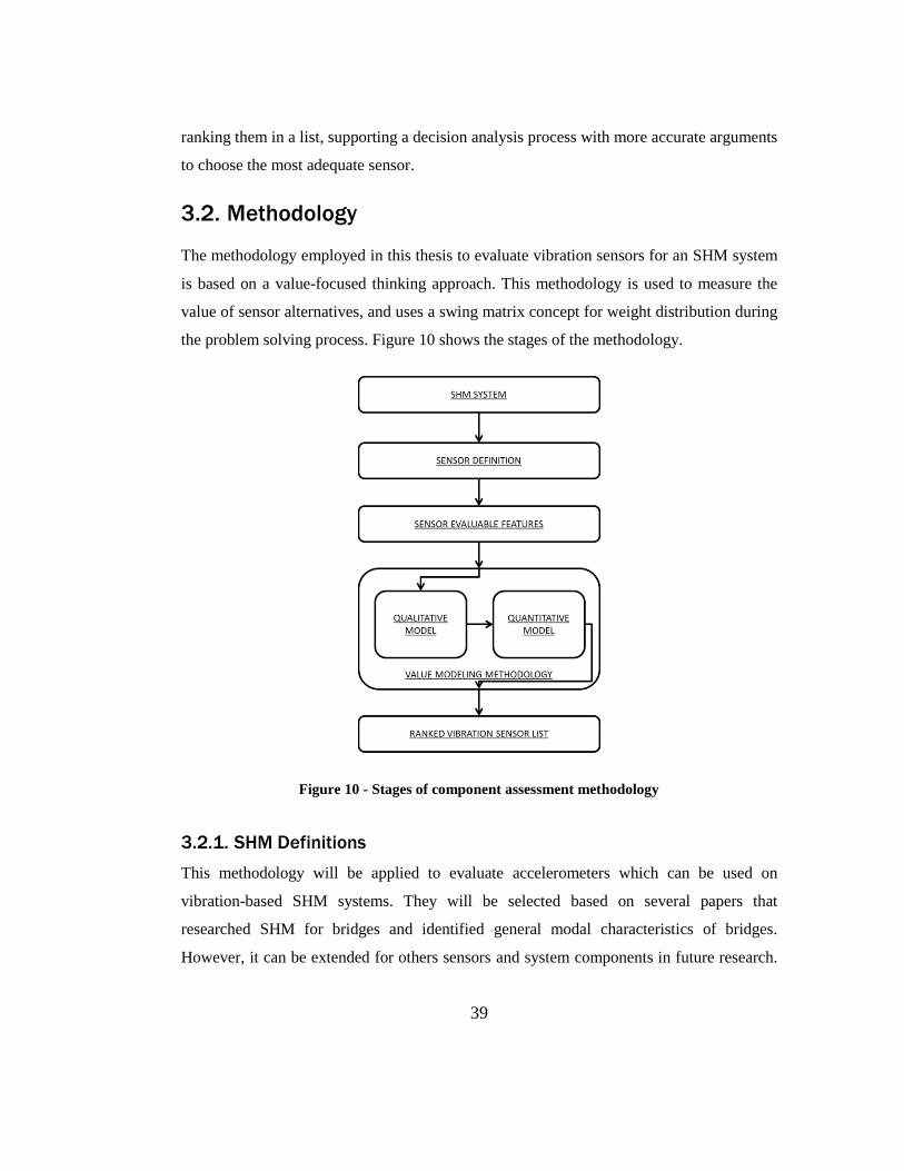
39
ranking them in a list, supporting a decision analysis process with more accurate arguments
to choose the most adequate sensor.
3.2. Methodology
The methodology employed in this thesis to evaluate vibration sensors for an SHM system
is based on a value-focused thinking approach. This methodology is used to measure the
value of sensor alternatives, and uses a swing matrix concept for weight distribution during
the problem solving process. Figure 10 shows the stages of the methodology.
Figure 10 - Stages of component assessment methodology
3.2.1. SHM Definitions
This methodology will be applied to evaluate accelerometers which can be used on
vibration-based SHM systems. They will be selected based on several papers that
researched SHM for bridges and identified general modal characteristics of bridges.
However, it can be extended for others sensors and system components in future research.

40
Presently, there are not any specific bridge SHM systems deployed in Brevard County
which count on with collaboration of Florida Tech researchers. Thus, it was decided to use
data from other vibration-based SHM systems, extracting data from research papers. The
advantage will be the application of this methodology observing general features of the
SHM systems.
Table 1 details some modal features of the selected bridges which had installed a SHM
system. It includes the bridges’ name, location, number of spans, length, and modal
frequencies researched and the maximum measured acceleration on the bridge by
researchers. This set of information will be used to select the accelerometers which will be
assessed by the methodology proposed. The table confirms the low modal frequencies of
the bridges which demand accelerometers that operate at low frequencies with high
resolution.
3.2.2. Sensor Definitions
The type of sensor selected was the accelerometer because they are the most employed
sensor in SHM to measure bridge vibrations. Data sheet specifications, which are also the
evaluated features that will be used to assess the sensors, are the following:
• Amplitude Range (Bandwidth): This is the operational frequency range of the sensor. The
lower amplitude range is the lowest measurable vibration level. Thus, the low frequency
accelerometers have their amplitude range starting at, if not, very close to, DC level [60].
• Measurement Range (Acceleration): This is the acceleration range that the sensor is able
to measure. It is the rate of change of velocity (the derivative of velocity) with respect to
time, and the unit is gravity “g” [60].
• Operating Temperature: This is the temperature range that the device will meet according
to the performance specifications. Accelerometers with internal electronics are more
sensitive to high temperature; however, the working temperature ranges usually exceed the
typical temperature environment [44].

41
• Resolution: It is the minimum detectable value of the intended input, which means the
smallest detectable increment in acceleration. The measurement resolution determines
noise density and the operating bandwidth typical of the accelerometer. When the
accelerometer has an output filter, the filter constant C should be considered. The
resolution is calculated by the following equation [60]:
𝑅 = 𝑁𝐷𝑒𝑛 × √𝐵𝑊𝑇𝑌𝑃 × 𝐶𝐹𝑖𝑙𝑡𝑒𝑟 , (3.1)
where N is the power spectral density noise in 𝜇𝑔 ⁄ √𝐻𝑧, which is another characteristic of
the accelerometer.
• Sensitivity: It is the response of the sensor to inputs, yielding on output the voltage
change per unit of acceleration (mV/g) [60]. Sensors with higher sensitivity have a greater
signal-to-noise ratio which favors sensors less susceptible electrostatically or
electromagnetically [44].
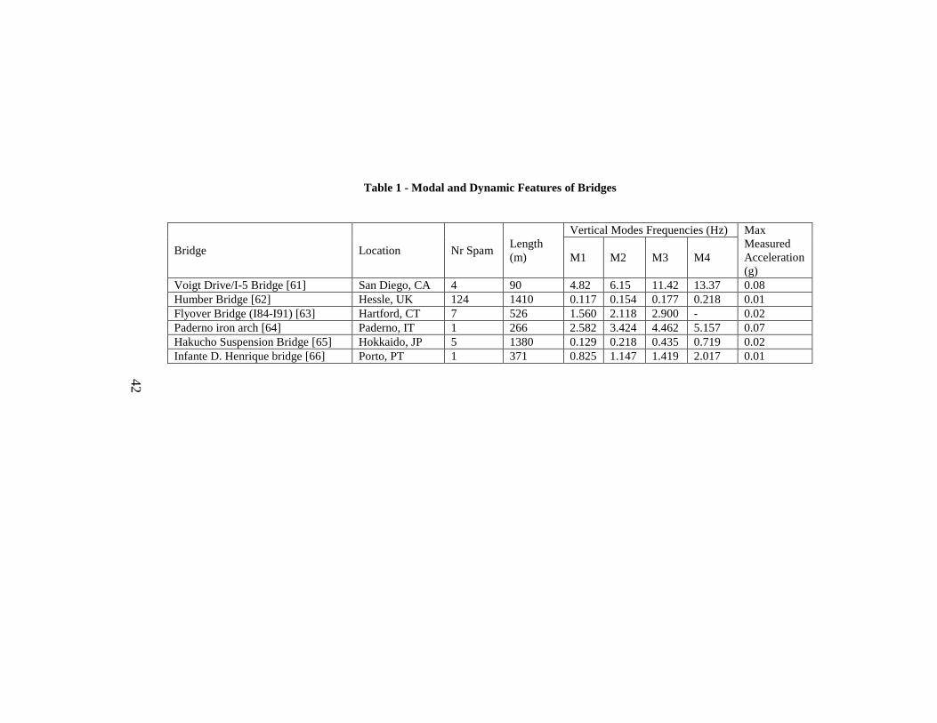
42
Table 1 - Modal and Dynamic Features of Bridges
Bridge Location Nr Spam Length
(m)
Vertical Modes Frequencies (Hz) Max
Measured
Acceleration
(g) M1 M2 M3 M4
Voigt Drive/I-5 Bridge [61] San Diego, CA 4 90 4.82 6.15 11.42 13.37 0.08
Humber Bridge [62] Hessle, UK 124 1410 0.117 0.154 0.177 0.218 0.01
Flyover Bridge (I84-I91) [63] Hartford, CT 7 526 1.560 2.118 2.900 - 0.02
Paderno iron arch [64] Paderno, IT 1 266 2.582 3.424 4.462 5.157 0.07
Hakucho Suspension Bridge [65] Hokkaido, JP 5 1380 0.129 0.218 0.435 0.719 0.02
Infante D. Henrique bridge [66] Porto, PT 1 371 0.825 1.147 1.419 2.017 0.01
42
AA

43
3.3. Value Modeling
Value modeling is a methodology used by systems engineers to provide an initial method
for evaluating candidate solutions [59] with multiple and, usually, conflicting objectives
[67]. It employs the concepts of value-focused thinking, which is a philosophy, among
others, to guide decision makers, and it is focused on the values or objectives that support
the decision. The value-focused thinking is based on three major principles: start with
values, use values to generate better alternatives, and use values to evaluate those
alternatives [68]. For the problem of multiple and, usually, conflicting objectives, value-
focused thinking recommends focusing first to fulfill, rather than on the alternatives. With
this methodology the mathematical framework of the value model is built, using the
concepts of multiple objective decision analysis (MODA) [59], and it is applied to
determine the best alternative among multiple conflicting objectives [68].
These concepts were used to develop a qualitative value model aiming to extract the most
important functions and objectives able to describe the analyzed sensors. The qualitative
value model served as a base to build the quantitative value model. That model results in a
method with efficient tools which provide an evaluation of the candidate solutions to figure
out how close they are to the fundamental objective defined in the qualitative model. Thus,
employing the value modeling methodology allows the development of the qualitative and
quantitative value models. The qualitative value model is the most important because it
reflects the key values that better characterize the sensor [59]. On the other hand, where the
qualitative model does not correctly capture these values, the quantitative value model will
not be suitable in evaluating sensors candidate solutions.
This thesis develops the value model that provides an unbiased, transparent, logical
structure to give a numerical overall value for each alternative of the vibration sensor
classification problem. Thus, the value model is built in five steps: (1) definition of
objectives and a functional value hierarchy that describes and organizes the objectives; (2)
definition of value measures that quantify each objective; (3) specification of ranges for
each of the value measures, from minimum acceptable (or available) to best possible (or
achievable); (4) definition of value functions to describe how each value measure

44
accumulates from low to high levels; and (5) definition of weights of the swing matrix to
specify the relative value of each value measure.
The value model which will be developed is basically a value hierarchy model added to
weights and single dimensional value functions. The evaluation measures and their single
dimensional value functions can be developed from several reliable sources, such as
literature, project documentation, stakeholders, and specialists. Hence, in this thesis the
major data sources used to narrow the alternative to the potential sensors solution
candidates were from research on vibration based SHM systems detailed in several
journals to identify the main features considered in sensor choice.
3.3.1. Qualitative Value Model
The qualitative value model was developed to satisfy four basic criteria cited by Parnell
[68]: completeness, mutually exclusive, operability, and as small as possible.
Completeness considers all essential objectives, which are measureable values and
sufficient to perform the evaluation. The criteria where functions or value measures on the
same tier in the hierarchy did not overlap are treated as mutually exclusive, and also as
independent. When everyone who uses the value measures is able to interpret and easily
understand them in the same way, they are considered operable. Finally, the last criteria
limits the model’s size to be as small as possible, and it is applied to help the analysis to be
focused on the most significant value measures [59].
To build the value model it is necessary to determine the functions, objectives, and value
measures, where the last should have a value function and a defined scale for each one. To
determine these factors, research journals were analyzed to extract the data to perform the
task. Thus, the qualitative value model was developed following these basic steps:
1. Identify the Fundamental Objective
2. Identify Functions that Provide Value
3. Identify the Objectives that Define Value

45
4. Identify the Value Measures.
Figure 11 - Framework of qualitative value model
Applying the methodology for the problem to define the most adequate accelerometer to
monitor the bridge vibration movement in a SHM system, yielded an analysis on screening
criteria listed earlier which resulted on the following identified values:
1. The accelerometer sensitivity to structure vibrations should be as high as possible.
2. The accelerometer should to be able to measure a large change of structure
acceleration.
3. The lower frequencies of vibration detectable by the accelerometer should be as
small as possible.
4. The accelerometer should be able to increment the detectable acceleration with the
smallest value possible.

46
5. The accelerometer should to be able to operate in a wide range of environment
temperatures.
These five values can be converted to objectives, and they can be evaluated through the
value measures detailed in the qualitative value model in Figure 12. The fundamental
objective of this analysis provides a value model to obtain an accurate accelerometer able
to measure vibration movement of a bridge structure. In the second tier of the model, the
two functions are the main evaluated actions of the sensor. Then, in the objectives there are
the statements with a short description of values articulated. Finally, the five value
measures detail the quantitative features to evaluate how well an accelerometer attains the
stated objectives.
Figure 12 - Qualitative value model for accelerometer sensor
The objectives and related value measures depicted in Figure 12 are defined in sequence:

47
Objective 1.1 Maximize the sensitivity to structure vibration. The sensitivity of the
candidate solutions can be directly evaluated through data extracted from specifications of
the sensor.
Measure 1.1.1 Sensitivity. The sensitivity of accelerometers candidate solutions is
measured in mV/g, and it is the measurement of output voltage change per unit of input
acceleration, which means that the objective is to maximize the response of the sensor to
input.
Objective 1.2 Maximize the measure on change of the acceleration. The measurement
range of the candidate solutions can be directly evaluated through data extracted from
specifications of the sensor.
Measure 1.2.1 Acceleration measurement range. The measurement range of
accelerometers candidate solutions is measured in g, and it is the measurement of changes
in acceleration of the structure through being the objective to get sensors with a wide range
of measurement.
Objective 1.3 Minimize the frequency of vibration detectable. The lower frequency of
vibration detectable of the candidate solutions can be directly evaluated through data
extracted from bandwidth specifications of the sensor.
Measure 1.3.1 Lower frequency detectable. The lower frequency which accelerometers
candidate solutions can detect will be determined by the left side of frequency bandwidth
that is measured in Hz. The lower frequency capability of the sensor detects the low
vibrations present in bridge structures.
Objective 1.4 Minimize the increment of the acceleration. The value of the increment in
the acceleration measured of the candidate solutions can be directly evaluated through data
extracted from specifications of the sensor.
Measure 1.4.1 Resolution. The smallest detectable increment in measured acceleration by
accelerometers candidate solutions is determined through the frequency bandwidth and
48
spectral noise and is measured in µg. This measure is the smallest change in acceleration
unity that can be detected by the sensor.
Objective 2.1 Maximize the range of the operational temperature. The operational
temperature range of the candidate solutions can be directly evaluated through data
extracted from specifications of the sensor.
Measure 2.1.1 Temperature range. The range of the operational temperature of
accelerometers candidate solutions is measured in oF. In this temperature range, the sensor
will meet the performance specifications providing reliable measurements.
The value hierarchy model developed and detailed above contains the fundamental
objective of the sensor characterizing the reason of interest in the decision analysis. Then,
the functions, objectives, and value measures were defined with the aim to identify the
highest value among the candidate solution for the proposed sensor type. Nevertheless,
these objectives are not conclusive to identify the most adequate sensor, and the next step
applies the multi-objective decision analysis to attain a better balance between the
objectives.
This thesis assumes that there is no uncertainty about the outcome of each alternative of the
value hierarchy model. Moreover, it is assumed that the evaluation measures are
completeness, mutually exclusive, independent, and operable. These assumptions allow the
measurement of alternative, sensor properties for this thesis to be simpler than when
uncertainty is present. Thus, the independence assumption permits the use of an additive
value function as a mathematic model for the quantitative value model [67].
3.3.2. Quantitative Value Model
The value modeling has as input for the qualitative value model the characteristics of the
object under decision analysis, and it yields a value hierarchy model with functions,
objectives, and value measures through the qualitative analysis. The outcome of that step is
the basis for the development of quantitative value model, which gives the capability to
49
determine how well candidate solutions for the object in analysis attain the objectives of
qualitative value model.
Using the most common mathematical function used on multiple objective decision
analysis to assess the values of candidate solutions, the additive value function is the
mathematical base of the qualitative model, which will focus on the bottom tier of the
value hierarchy model. To employ the additive value function model, it is assumed that the
value measures are independent, which means that the assessment of the value function on
one value measure does not depend on the tier of the other value measures [67]. A value
function should be built for each candidate solution, converting its measured values to a
standard unit named “value”. In the value function, the value measures receive a weight
which highlight the importance and impact of the each value measures on the decision
analysis of the problem [59]. The following equation is the mathematical representation of
the additive value function, and it is used to calculate the value of the value measure [67].
Thus, the form of the value function, v(x),
𝑣(𝑥) =∑𝑤𝑖𝑣𝑖(𝑥𝑖)
𝑛
𝑖=1
, (3.2)
where for a set of value measure given by vector x,
v(x) is the alternative’s value of x,
i = 1 to n is the index of the value measure,
xi is the score of the ith value measure,
vi (xi) is the single-dimensional value function of of xi,
wi is the swing weight of the ith value measure,
and

50
∑𝑤𝑖 = 1
𝑛
𝑖=1
(3.3)
With weights and single dimensional value functions correctly estimated, an overall value
of each candidate solution can be determined.
3.3.2.1. Single-Dimensional Value Functions
To calculate the value function v(x) of the candidate solution defined in Eq. 3.2, it is
necessary to transform the value measure of each objective, which has its specific
measurement scale. This is performed by converting the value measures to a standard unit
using the single-dimensional value function. In this single value function, the x-axis is the
scale of the value measure, and the y-axis is a standard unit of value which can use the
scale of 0 to1, 0 to 10, or 0 to 100, and the choice is made on basis of which is more
appropriate for decision makers.
The single-dimensional value functions measure returns to scale on the value measures,
and they can have any shape, but in practice they are mostly plotted in four basic shapes:
linear, concave, convex, and S-curve. These value functions typically present a monotonic
behavior, increasing or decreasing, aligned with the aim of maximizing or minimizing the
objective, respectively. Measuring the return to scale on the value measure, these value
functions can vary the output with the change in input value among constant (or linear)
returns to scale (CRS), decrease returns to scale (DRS), and increasing returns to scale
(IRS). In the constant returns to scale, the output increases or decreases by the same
proportional change as all inputs change. In the decrease returns to scale, the output
decreases more than proportional change in input. In the increasing returns to scale, the
input increases more than that proportional change in inputs.
Thus, the linear, concave, and convex shapes of the single-dimensional value functions
have a behavior CRS, DRS, and IRS, respectively. The exception is the S-curve because it
presents the IRS and DRS characteristics due to it being the consequence of a combination
of two measures [67].

51
Figure 13 - Typical shapes of value function [59]
Figure 13 shows the most common shapes of value functions, where the curves on the right
are monotonically decreasing, and on left they are monotonically increasing. The
techniques to develop the shape of value curves were presented by Kirkwood [69], and it
was concluded that the exponential value function is the most reasonable shape to plot that
curve, and that the value function cannot generally be treated as a simple linear function.
The exponential Eq. 3.4 has a particular form as depicted below. It depends on the

52
exponential constant ρ and on the range of the evaluation measure, which are represented
by the high value xH and the low value xL. The exponential constant ρ is responsible for
determining the shape of the value function, so that when the constant ρ is infinity, the
exponential value function tends to assume a linear shape. Thus, the exponential single
dimensional value function v(x) can be written as follows [70]:
𝑣(𝑥) =
{
1 − exp [−(𝑥 − 𝑥𝐿)/𝜌]
1 − exp [−(𝑥𝐻 − 𝑥𝐿)/𝜌] , 𝜌 ≠ ∞
𝑥 − 𝑥𝐿𝑥𝐻 − 𝑥𝐿
, 𝑜𝑡ℎ𝑒𝑟𝑤𝑖𝑠𝑒 (3.4)
The Eq. 3.4 is the value function that plots a shape monotonically increasing over x-axis,
which is applied when the objective is maximizing higher values of x, which is preferred
more than the lower values. When it is needed to plot a shape of a value measure that is
monotonically decreasing over x-axis, where the objective is minimizing lower amounts of
x, the exponential value function v(x) can be written as follows [70]:
𝑣(𝑥) =
{
1 − exp [−(𝑥𝐻 − 𝑥)/𝜌]
1 − exp [−(𝑥𝐻 − 𝑥𝐿)/𝜌] , 𝜌 ≠ ∞
𝑥𝐻 − 𝑥
𝑥𝐻 − 𝑥𝐿 , 𝑜𝑡ℎ𝑒𝑟𝑤𝑖𝑠𝑒
(3.5)
The exponential constant ρ can be determined based on the concept of the mid-value, xm,
for the range of evaluation measure and by using the normalized exponential constant, R.
The mid-value is defined by the difference between the lowest score in the range and the
mid-value which is the same as the difference between the mid-value and the highest score
53
in the range, and it is used to calculate the z0.5, which is the normalized value of xm. The
exponential constant is calculated in the equation below [70]:
𝜌 = 𝑅( 𝑥𝐻 − 𝑥𝐿 ) (3.6)
To determine the exponential constant R, it is necessary to calculate the value of z0.5, the
normalized value of mid-value, using the following expression:
𝑧0.5 = 𝑥𝑚 − 𝑥𝐿𝑥𝐻 − 𝑥𝐿
(3.7)
With z0.5 calculated and given that v(xm)=0.5 due xm is the mid-value range of evaluation
measure, the normalized constant R can be determined using the Eq. 3.8 [70] or through
the table in Figure 14 by looking at the z0.5 value.
𝑣(𝑥𝑚) = 0.5 =1 − exp [−(−
𝑧0.5𝑅⁄ )]
1 − exp [−1 𝑅⁄ ] (3.8)
Hence, the value of exponential constant ρ can be determined finding the mid-value for the
interval between the lower, xL, and higher, xH, value measure, also known as evaluation
measures. Thus, the constant ρ will vary within realistic values depending on the range of
evaluation measures. Figure 15 exemplifies values of ρ and how it influences the shape of
curve. Another aspect of that constant is whether the magnitude of ρ is less than 0.1 × (xH −
xL), then the shape of the value function will be so curved as to indicate that there is some
highly unusual situation. Whether the magnitude of ρ is greater than 10 × (xH − xL), then
the value function will be essentially a straight line. Therefore, the realistic values of ρ
should be greater than 1/10 the range of the evaluation measure [70].

54
Figure 14 - Values of normalized exponential constant R[69]

55
Figure 15 - Examples of exponential single-dimensional value functions for different values of
the exponential constant ρ: (a) monotonically increasing preferences and (b) monotonically
decreasing preferences [70]
3.3.2.2. Swing Weight Matrix
After determining the single-dimensional value functions, the next step in the value
modeling process is determining the weights wi (Eq 3.3), once the weights have a key role

56
in the additive value model to complete the specification of the value function [70].
Applying the multiple objective decision analysis (MODA) quantitative assessment
characteristics, by evaluating the value measures and converting them into standard values
with single-dimensional value functions and weighting them to scale the importance of
each value measure, it is possible to assess the tradeoff between the objectives defined in
qualitative value model [68].
In the weighting process, two properties of value function defined by Kirkwood [70]
should be considered due to their importance in the procedure for determining the weights:
1. The single-dimensional value functions are specified so that each one is equal to
zero for the least preferred level that is being considered for the corresponding
evaluation measure [70].
2. Each of the single-dimensional value functions is specified so that it is equal to one
for the most preferred level that is being considered for the corresponding
evaluation measure [70].
Thus, analyzing the MODA concepts and these properties of the single-dimensional value
functions, it is possible to determine that the weights depend on the range and the
importance of the measure scale. Hence, the weight distribution process should increment
in value from the least preferred to most preferred value measure [70]. These points
provide the basis to develop the swing weight matrix, which is a method used to determine
the weight [68].
The swing weight matrix is a method designed provide a better visualization of how the
weights were distributed for decision makers, helping to make more clear the importance
and impact of each value measure range in the decision analysis [67]. Thus, the swing
weight matrix clearly delineates the two major weighting features: importance (large,
moderate, small) and variability (high, medium, low), prior to the weighting assessment
[68]. The concept behind the swing weight matrix, detailed in Table 2, is straightforward,
and it applies the concepts recently analyzed.

57
Table 2 - The Elements of the Swing Weight Matrix [67]
Importance of the Value Measure to the Decision
(Intuitive Judgment)
Critical
(High)
Important
(Medium)
Enablers
(Low)
Impact of the range of
the value measure on
the decision (factual
judgment)
Large A B2 C3
Moderate B1 C2 D2
Small C1 D1 C
The swing weight matrix has on the top scale the definition of value measures’ importance
for the decision analysis, and the left scale defines the impact of changing the value
measure range on the decision. Hence, the value measure is most important, producing
large impacts for decisions, and should be placed in the upper left corner; the less
important ones, which produce small impacts on decisions, should be placed in the lower
right corner of the matrix[67]. The matrix is usually shown in 3×3 dimensions, but if it is
necessary, a 5×5 matrix can be used on cases that demand higher levels of discrimination
between value measures [59].
The process of distribution of non-normalized weights should be made moving in a
diagonal direction from the top left to the bottom right of the swing weight matrix, and the
magnitude of weights, for more consistency on weighting distribution, need to follow the
strict relationships detailed in inequalities below [59]:
A > all other cells (3.9)
B1 > C1, C2, D1,D2, E (3.10)
B2 > C2, C3, D1,D2, E (3.11)
C1 > D1, E (3.12)

58
D1 > E (3.13)
D2 > E (3.14)
The weights are distributed following the methodology proposed by Trainor [59], which
follows the value increment approach [69], where the cell A (in the upper left corner) is
assigned with an arbitrary non-normalized swing weight of 100, and the cell E (in the
lower right corner) with the lowest weight of 1. The other seven non-normalized swing
weights are assigned weights relative to the weight 100, going from the very important
factors to the less important factors.
The swing weights should be normalized using the Eq. 3.15, which converts them in
measure weights on a scale of 0.0–1.0. The measure weights also are known as global
weights. Thus, to obtain the normalized weighting of value measures in the quantitative
value model, the weights in the swing matrix are normalized using the following
expression [59]:
𝑤𝑖 =𝑓𝑖
∑ 𝑓𝑖𝑛𝑖=1
, (3.15)
where fi is the non-normalized swing weight assessed for the ith value measure, i = 1 to n
for the number of value measures, and wi are the normalized swing weights [67].

59
Chapter 4 METHODS AND RESULTS
4.1. Introduction
This chapter will apply the value modeling methodology presented earlier, which is
focused on supporting the decision making process. This thesis discusses the SHM systems
to be applied in bridge monitoring as well as the current assessment methodology to
provide a tool, at the systems engineering level, which allows the evaluation of the
candidate solution to be used as a component of the bridges’ SHM system. The value
modeling methodology can be performed through two distinct models, the qualitative value
model and the quantitative value model. The first model was discussed in section 3.3.1 and
its outcome was a model that defined the fundamental objective, identified the functions,
objectives, and value measures, all of which are depicted in Figure 12. With information
from the qualitative value model, the quantitative value model will be developed.
Starting with the selection of accelerometers that will be treated as candidate solutions, the
candidate solutions’ raw data then will be gathered from specifications detailed on data
sheets. Then the value functions for each value measure and the swing matrix will be
determined, and from them, the final weighted values for each candidate solution will be
determined.
4.2. Sensor Selection
Twenty accelerometers were chosen as candidate solutions, and their selected features data
will be analyzed with value modeling methodology. The first ten sensors were selected
from research papers involved with bridges’ SHM, where there are cases of SHM analyzed
in laboratories (01, 02, 07 and 08) and systems deployed on bridges (03, 04, 05, 06, 09, and

60
10). This selection was limited by the difficulty of finding the specification of sensors in
many papers. The other ten accelerometers were selected through research of
manufacturers’ websites and they were chosen on the basis of specifications of the first
nine and of the sensors’ features demanded by bridges’ SHM. Table 3 below details the
accelerometer which will be analyzed.
Table 3 - Candidate Solutions for Accelerometer Sensor
Cand Sol Nr SHM research Manufacturer Model
01 TestBed UCSD [61] crossbow CXL01LF1
02 TestBed UCSD [61] PCB 3801G3FB3G
03 Infante D. Henrique bridge [66] Kinemetrics ES-U2
04 Yongjong Grand Bridge [71] NewConsTech AC310-002
05 Paderno iron arch bridge [64] Wilcoxon WR-731A
06 Sunrise Boulevard Bridge [72] PCB 603C01
07 TestBed QUT [39] PCB 393B05
08 TestBed KU Leuven [73] PCB 333B
09 University of Porto footbridge [74] PCB 393C
10 Bridge over Skidträsk River [75] Colibrys SF1500S
11 - PCB 622B01
12 - PCB 626B02
13 - Dytran 3166B1
14 - Endevco 7251HT10
15 - Endevco 752A13
16 - Kistler 8640A10
17 - Kistler 8312A2
18 - CTC AC212
19 - CTC AC133
20 - ASC GmbH P101A15
With the selected sensors, the next step was to determine the ranges of variation for the
parameters of the functions. This analysis was based on several information sources, such
as research, history of ambient temperatures, and regulatory agencies. The values are
defined in Table 4. A consideration when setting the initial frequency of operation is that
the accelerometer should be able to detect frequencies from 0 Hz (DC) because the bridges
are the lower frequencies, a modal characteristic, so this value was considered ideal and
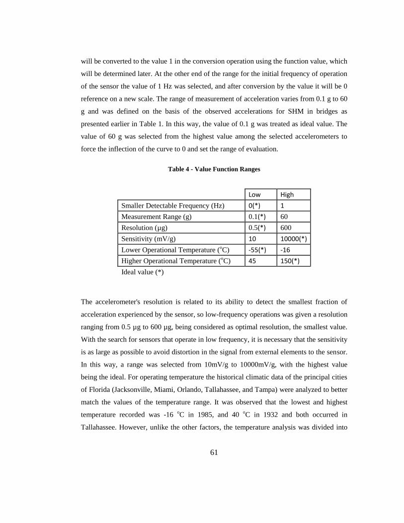
61
will be converted to the value 1 in the conversion operation using the function value, which
will be determined later. At the other end of the range for the initial frequency of operation
of the sensor the value of 1 Hz was selected, and after conversion by the value it will be 0
reference on a new scale. The range of measurement of acceleration varies from 0.1 g to 60
g and was defined on the basis of the observed accelerations for SHM in bridges as
presented earlier in Table 1. In this way, the value of 0.1 g was treated as ideal value. The
value of 60 g was selected from the highest value among the selected accelerometers to
force the inflection of the curve to 0 and set the range of evaluation.
Table 4 - Value Function Ranges
Low High
Smaller Detectable Frequency (Hz) 0(*) 1
Measurement Range (g) 0.1(*) 60
Resolution (µg) 0.5(*) 600
Sensitivity (mV/g) 10 10000(*)
Lower Operational Temperature (oC) -55(*) -16
Higher Operational Temperature (oC) 45 150(*)
Ideal value (*)
The accelerometer's resolution is related to its ability to detect the smallest fraction of
acceleration experienced by the sensor, so low-frequency operations was given a resolution
ranging from 0.5 µg to 600 µg, being considered as optimal resolution, the smallest value.
With the search for sensors that operate in low frequency, it is necessary that the sensitivity
is as large as possible to avoid distortion in the signal from external elements to the sensor.
In this way, a range was selected from 10mV/g to 10000mV/g, with the highest value
being the ideal. For operating temperature the historical climatic data of the principal cities
of Florida (Jacksonville, Miami, Orlando, Tallahassee, and Tampa) were analyzed to better
match the values of the temperature range. It was observed that the lowest and highest
temperature recorded was -16 oC in 1985, and 40
oC in 1932 and both occurred in
Tallahassee. However, unlike the other factors, the temperature analysis was divided into

62
two parts to better evaluate the sensors: lower operating temperature and higher operating
temperature. In this way, it was found that the lower temperature should range between -55
oC and -16
oC and between 45
oC and 150
oC to the upper range. The ideal values selected
were of -55 oC and 150
oC. Table 5 details the scores, value measures, and respective
dimensions for each candidate solution.
Table 5 - Raw Data Matrix
Cand Sol Nr
Value Measure
Smaller
Detectable
Frequency
(Hz)
Measurement
Range
(g)
Resolution
(µg)
Sensitivity
(mV/g)
Operating
Temperature
Range
(oC)
Low High
01 0 (DC) 1 500 2000 -40 85
02 0 (DC) 3 60 1000 -40 85
03 0 (DC) 0.25 0.5 2500 -20 70
04 0 (DC) 2 13 2000 -40 80
05 0.05 0.5 0.5 10000 -10 65
06 0.5 50 350 100 -54 121
07 0.2 0.5 4 10000 -18 80
08 0.5 50 150 100 -18 66
09 0.025 2.5 100 1000 -55 150
10 0 (DC) 3 0.5 1200 -40 85
11 0.2 50 50 100 -54 121
12 0.2 10 20 500 -54 121
13 0.3 10 80 500 -51 121
14 0.2 10 300 500 -55 150
15 0.3 5 50 1000 -20 85
16 0.5 10 160 500 -40 65
17 0 (DC) 2 540 1000 -40 85
18 0.2 30 6 250 -50 121
19 0.1 10 5 500 -50 121
20 0.3 50 400 100 -55 125
Ideal value 0 (DC) 0.1 0.5 10000 -55 150
Rejected value 1 60 600 10 -16 45

63
4.3. Developing Value Functions
With the raw data from candidate solutions and the value measures variation ranges
determined, the next step of methodology will be developing the value function for each
objective defined on qualitative value model described on Section 3.3.1. Appling the value
function to raw data will convert them into value between 0 and 1, with 0 being the worst
possible value, and 1 being the best possible value.
The value functions were developed using the equations shown in Section 3.3.2.1. Each
objective was analyzed to determine the behavior of the value measure relative to
fundamental objective. This means determining if the slope of the value functions for a
specific value measure should be characterized as monotonically increasing or decreasing.
This analysis impacted on which equation was used to determine the value function and the
results are shown in Table 6. The analysis was performed through the definition of the
ideal and the unwished values for each objective. These values are placed on the last two
rows of the Table 5. Thus, the objectives 1.1.1, 2.1.1 (b) applied the Equation 3.4, and the
objectives 1.2.1, 1.3.1, 1.4.1, and 2.1.1 (a) applied the Equation 3.5.
Determining the direction of slope of the value function is needed to calculate the other
parameters which characterize each function for its respective objective. Then, it is
necessary to figure out the value of the exponential constant, ρ. This parameter is
calculated using the Equation 3.6. To calculate the constant, ρ, it is necessary to determine
the values of maximum and minimum value measure to assure that the results of the value
function are restricted between the range of 0 and 1. These values are the xH and xL,
respectively, and they were set up with the value measures ideal and unwished. The last
factor necessary to calculate the constant, ρ, is the normalized exponential constant, R. This
constant is obtained from the table shown on Figure 14 or through the equation 3.8, but for
both the calculation of the z0.5 is mandatory. To figure out the normalized mid-value of the
data set required calculating the mid-value range of the value measure xm. The mid-value
for each value measure was calculated based on the frequency of values into the data set
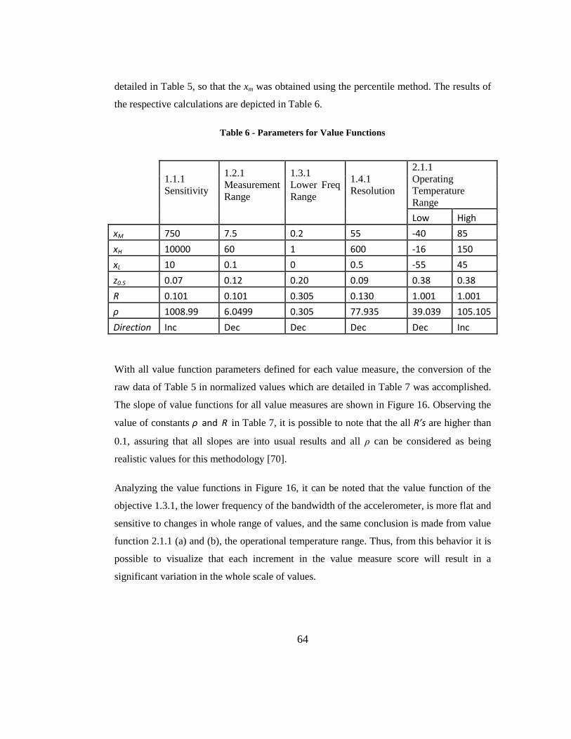
64
detailed in Table 5, so that the xm was obtained using the percentile method. The results of
the respective calculations are depicted in Table 6.
Table 6 - Parameters for Value Functions
1.1.1
Sensitivity
1.2.1
Measurement
Range
1.3.1
Lower Freq
Range
1.4.1
Resolution
2.1.1
Operating
Temperature
Range
Low High
xM 750 7.5 0.2 55 -40 85
xH 10000 60 1 600 -16 150
xL 10 0.1 0 0.5 -55 45
z0.5 0.07 0.12 0.20 0.09 0.38 0.38
R 0.101 0.101 0.305 0.130 1.001 1.001
ρ 1008.99 6.0499 0.305 77.935 39.039 105.105
Direction Inc Dec Dec Dec Dec Inc
With all value function parameters defined for each value measure, the conversion of the
raw data of Table 5 in normalized values which are detailed in Table 7 was accomplished.
The slope of value functions for all value measures are shown in Figure 16. Observing the
value of constants ρ and R in Table 7, it is possible to note that the all R’s are higher than
0.1, assuring that all slopes are into usual results and all ρ can be considered as being
realistic values for this methodology [70].
Analyzing the value functions in Figure 16, it can be noted that the value function of the
objective 1.3.1, the lower frequency of the bandwidth of the accelerometer, is more flat and
sensitive to changes in whole range of values, and the same conclusion is made from value
function 2.1.1 (a) and (b), the operational temperature range. Thus, from this behavior it is
possible to visualize that each increment in the value measure score will result in a
significant variation in the whole scale of values.

65
Figure 16 - Value functions for all value measures of the analyzed sensor
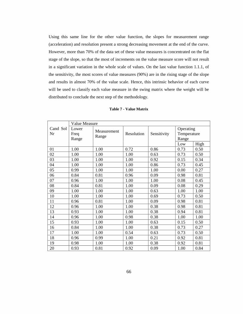
66
Using this same line for the other value function, the slopes for measurement range
(acceleration) and resolution present a strong decreasing movement at the end of the curve.
However, more than 70% of the data set of these value measures is concentrated on the flat
stage of the slope, so that the most of increments on the value measure score will not result
in a significant variation in the whole scale of values. On the last value function 1.1.1, of
the sensitivity, the most scores of value measures (90%) are in the rising stage of the slope
and results in almost 70% of the value scale. Hence, this intrinsic behavior of each curve
will be used to classify each value measure in the swing matrix where the weight will be
distributed to conclude the next step of the methodology.
Table 7 - Value Matrix
Cand Sol
Nr
Value Measure
Lower
Freq
Range
Measurement
Range Resolution Sensitivity
Operating
Temperature
Range
Low High
01 1.00 1.00 0.72 0.86 0.73 0.50
02 1.00 1.00 1.00 0.63 0.73 0.50
03 1.00 1.00 1.00 0.92 0.15 0.34
04 1.00 1.00 1.00 0.86 0.73 0.45
05 0.99 1.00 1.00 1.00 0.00 0.27
06 0.84 0.81 0.96 0.09 0.98 0.81
07 0.96 1.00 1.00 1.00 0.08 0.45
08 0.84 0.81 1.00 0.09 0.08 0.29
09 1.00 1.00 1.00 0.63 1.00 1.00
10 1.00 1.00 1.00 0.69 0.73 0.50
11 0.96 0.81 1.00 0.09 0.98 0.81
12 0.96 1.00 1.00 0.38 0.98 0.81
13 0.93 1.00 1.00 0.38 0.94 0.81
14 0.96 1.00 0.98 0.38 1.00 1.00
15 0.93 1.00 1.00 0.63 0.15 0.50
16 0.84 1.00 1.00 0.38 0.73 0.27
17 1.00 1.00 0.54 0.63 0.73 0.50
18 0.96 0.99 1.00 0.21 0.92 0.81
19 0.98 1.00 1.00 0.38 0.92 0.81
20 0.93 0.81 0.92 0.09 1.00 0.84
67
4.4. Assigning Weights on Swing Matrix
The last step of the methodology is the application of the swing matrix method to assess
weights for different objectives based on two main aspects: the importance of the objective
for the mission and the impact of the amount of variation of the value measure in the scale
of normalized values. The rules to complete the swing matrix were detailed in Section
3.3.2.2. It developed five objectives that should be distributed on a swing matrix, observing
their importance for the mission and impact on scale value.
It was considered as critical for the mission that the features demand more accuracy of the
sensor, and classified into this area were the lower frequency of operation and the
resolution of the accelerometer. The sensitivity and measurement range were classified as
important for the mission because they are chosen according to the frequency of the sensor
and bridge structure. The temperature range was classified as enabler, due to it not
participating directly oin measurement, but it enables the accelerometer to operate under
specified environmental conditions.
The other classification factor, the impact of the range, was made based on results of the
value functions graph in Figure 16, and on the analysis performed about the behavior of
their slopes in the last section. The analysis key for this classification was how the selected
value measure range is related to the normalized value range by value function. Hence, it
was classified as having a large impact on scale of value in the lower frequency of the
bandwidth of the accelerometer and the operational temperature range due to the almost
linearity of graph behavior in all value measure ranges. The measurement range and
resolution were classified as yielding a small impact because most parts of the data set of
value measure of selected accelerometers are located on flat area of the graph, and they
will not yield much variance on normalized values. Finally, the sensitivity was classified as
having a medium impact on value because most accelerometers are concentrated under the
rising stage of the slope of its value function graph. The swing matrix is depicted in Table
8.
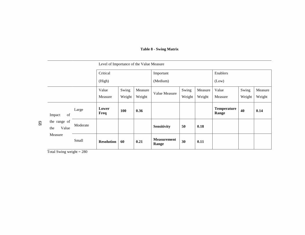
68
Table 8 - Swing Matrix
Level of Importance of the Value Measure
Critical
(High)
Important
(Medium)
Enablers
(Low)
Value
Measure
Swing
Weight
Measure
Weight Value Measure
Swing
Weight
Measure
Weight
Value
Measure
Swing
Weight
Measure
Weight
Impact of
the range of
the Value
Measure
Large Lower
Freq 100 0.36
Temperature
Range 40 0.14
Moderate Sensitivity 50 0.18
Small Resolution 60 0.21 Measurement
Range 30 0.11
Total Swing weight = 280
68
AA
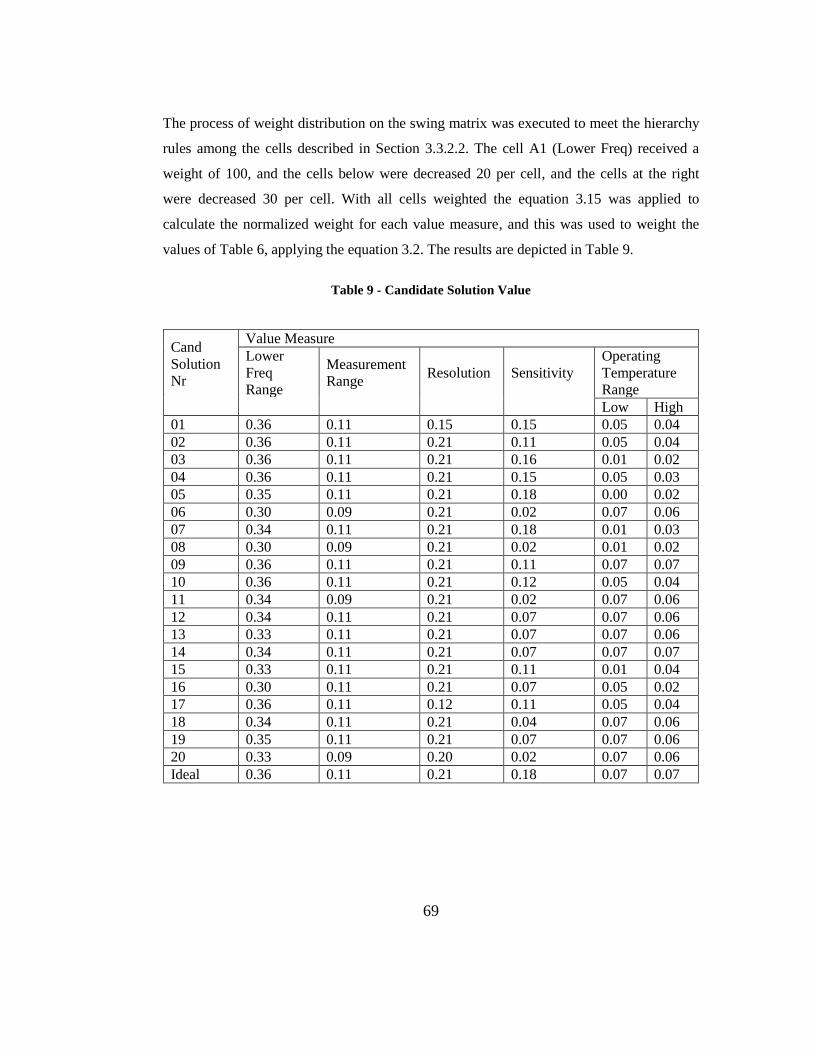
69
The process of weight distribution on the swing matrix was executed to meet the hierarchy
rules among the cells described in Section 3.3.2.2. The cell A1 (Lower Freq) received a
weight of 100, and the cells below were decreased 20 per cell, and the cells at the right
were decreased 30 per cell. With all cells weighted the equation 3.15 was applied to
calculate the normalized weight for each value measure, and this was used to weight the
values of Table 6, applying the equation 3.2. The results are depicted in Table 9.
Table 9 - Candidate Solution Value
Cand
Solution
Nr
Value Measure
Lower
Freq
Range
Measurement
Range Resolution Sensitivity
Operating
Temperature
Range
Low High
01 0.36 0.11 0.15 0.15 0.05 0.04
02 0.36 0.11 0.21 0.11 0.05 0.04
03 0.36 0.11 0.21 0.16 0.01 0.02
04 0.36 0.11 0.21 0.15 0.05 0.03
05 0.35 0.11 0.21 0.18 0.00 0.02
06 0.30 0.09 0.21 0.02 0.07 0.06
07 0.34 0.11 0.21 0.18 0.01 0.03
08 0.30 0.09 0.21 0.02 0.01 0.02
09 0.36 0.11 0.21 0.11 0.07 0.07
10 0.36 0.11 0.21 0.12 0.05 0.04
11 0.34 0.09 0.21 0.02 0.07 0.06
12 0.34 0.11 0.21 0.07 0.07 0.06
13 0.33 0.11 0.21 0.07 0.07 0.06
14 0.34 0.11 0.21 0.07 0.07 0.07
15 0.33 0.11 0.21 0.11 0.01 0.04
16 0.30 0.11 0.21 0.07 0.05 0.02
17 0.36 0.11 0.12 0.11 0.05 0.04
18 0.34 0.11 0.21 0.04 0.07 0.06
19 0.35 0.11 0.21 0.07 0.07 0.06
20 0.33 0.09 0.20 0.02 0.07 0.06
Ideal 0.36 0.11 0.21 0.18 0.07 0.07
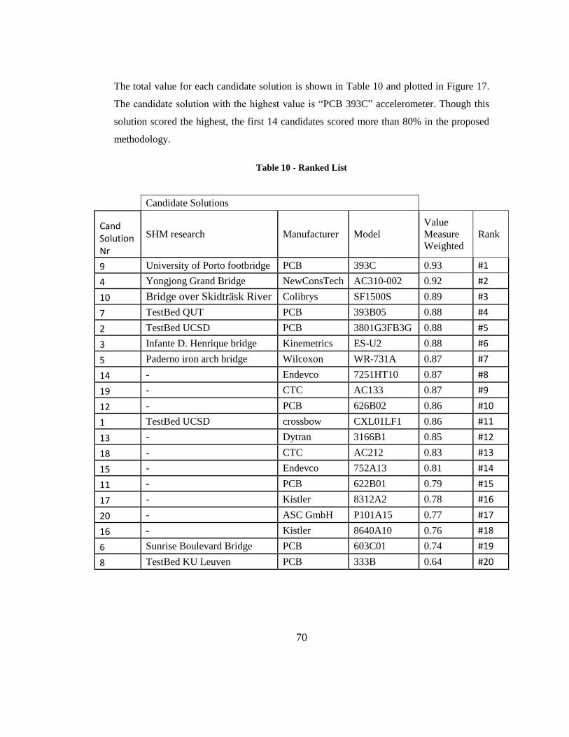
70
The total value for each candidate solution is shown in Table 10 and plotted in Figure 17.
The candidate solution with the highest value is “PCB 393C” accelerometer. Though this
solution scored the highest, the first 14 candidates scored more than 80% in the proposed
methodology.
Table 10 - Ranked List
Candidate Solutions
Cand Solution Nr
SHM research Manufacturer Model
Value
Measure
Weighted
Rank
9 University of Porto footbridge PCB 393C 0.93 #1
4 Yongjong Grand Bridge NewConsTech AC310-002 0.92 #2
10 Bridge over Skidträsk River Colibrys SF1500S 0.89 #3
7 TestBed QUT PCB 393B05 0.88 #4
2 TestBed UCSD PCB 3801G3FB3G 0.88 #5
3 Infante D. Henrique bridge Kinemetrics ES-U2 0.88 #6
5 Paderno iron arch bridge Wilcoxon WR-731A 0.87 #7
14 - Endevco 7251HT10 0.87 #8
19 - CTC AC133 0.87 #9
12 - PCB 626B02 0.86 #10
1 TestBed UCSD crossbow CXL01LF1 0.86 #11
13 - Dytran 3166B1 0.85 #12
18 - CTC AC212 0.83 #13
15 - Endevco 752A13 0.81 #14
11 - PCB 622B01 0.79 #15
17 - Kistler 8312A2 0.78 #16
20 - ASC GmbH P101A15 0.77 #17
16 - Kistler 8640A10 0.76 #18
6 Sunrise Boulevard Bridge PCB 603C01 0.74 #19
8 TestBed KU Leuven PCB 333B 0.64 #20

71
From Figure 17, the contribution of lower frequency of the bandwidth stands out as the
most important impact for the candidate solution, followed by resolution, as expected by
weight distribution.
Figure 17 - Value Ranking by Candidate Solutions
72
4.5. Sensitive Analysis
The sensitive analysis was conducted to understand the behavior of weight when it is
swinging for each value measure. The weight was varying from 0 to 100, which is the
range before its normalization. However, it is relevant to note that when the weight assume
zero, the value measure has no more influence on the decision, and when it approaches a
high weight, the problem become less a decision analysis problem and more of an
optimization effort for the high weight value measures. All candidate solutions were
submitted to analysis which was focused to conclude over the whole set to understand the
general influence of each weight on decision analysis.
For each value measure, the analysis was performed in reference to the highest value
candidate solution, PCB 393C, and its original weight, so the others’ values were
calculated for estimated weights. Thus, for the low frequency, the weight base was 100, for
the resolution it was 60, so the same rule was applied for the others’ value measures. The
results are detailed in Table 11, Table 12,Table 13, Table 14, and Table 15 and their
respective graphs are in Figure 18, Figure 19, Figure 20, Figure 21, and Figure 22.
Looking at Table 11 and Figure 18, it is noted that the weight of PCB 393C is always the
highest value, regardless of the weight swinging. Thus, for the weight assessment of the
lower frequency value measure, the better candidate solution is not sensitive to the weight.
Also, it is possible to observe that there are no relevant changes in the candidate solutions
ranking which means that most of the candidates are not sensitive to this weight. It means
that no further analysis for optimizing this weight is necessary.
Analyzing the results in Table 12 and Figure 19, the behavior of the candidate solutions is
like the former analysis, with the weight of PCB 393C always being the highest value with
the weight swinging. Thus, for the weight assessment of the resolution value measure, the
better candidate solution is not sensitive to the weight, and there are no relevant changes in
the candidate solutions ranking, either.

73
Table 11 Sensitive Analysis for Lower Frequency Value Measure
Weight Analyzed
Nr Cand Solution
Cand Solution 0 20 40 60 80 100
1 CXL01LF1 0.78 0.80 0.82 0.84 0.85 0.86
2 3801G3FB3G 0.81 0.83 0.84 0.86 0.87 0.88
3 ES-U2 0.81 0.83 0.84 0.86 0.87 0.88
4 AC310-002 0.87 0.88 0.89 0.90 0.91 0.92
5 WR-731A 0.81 0.83 0.84 0.85 0.87 0.87
6 603C01 0.68 0.69 0.71 0.72 0.73 0.74
7 393B05 0.84 0.85 0.86 0.87 0.88 0.88
8 333B 0.53 0.56 0.59 0.61 0.63 0.64
9 393C 0.90 0.91 0.91 0.92 0.93 0.93
10 SF1500S 0.83 0.85 0.86 0.87 0.88 0.89
11 622B01 0.69 0.72 0.74 0.76 0.78 0.79
12 626B02 0.81 0.82 0.84 0.85 0.86 0.86
13 3166B1 0.80 0.81 0.83 0.83 0.84 0.85
14 7251HT10 0.82 0.84 0.85 0.86 0.87 0.87
15 752A13 0.75 0.77 0.78 0.79 0.80 0.81
16 8640A10 0.72 0.73 0.74 0.75 0.75 0.76
17 8312A2 0.66 0.69 0.72 0.74 0.76 0.78
18 AC212 0.75 0.77 0.79 0.80 0.82 0.83
19 AC133 0.80 0.82 0.83 0.85 0.86 0.87
20 P101A15 0.67 0.70 0.72 0.74 0.75 0.77
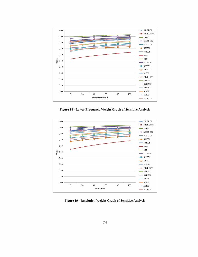
74
Figure 18 - Lower Frequency Weight Graph of Sensitive Analysis
Figure 19 - Resolution Weight Graph of Sensitive Analysis
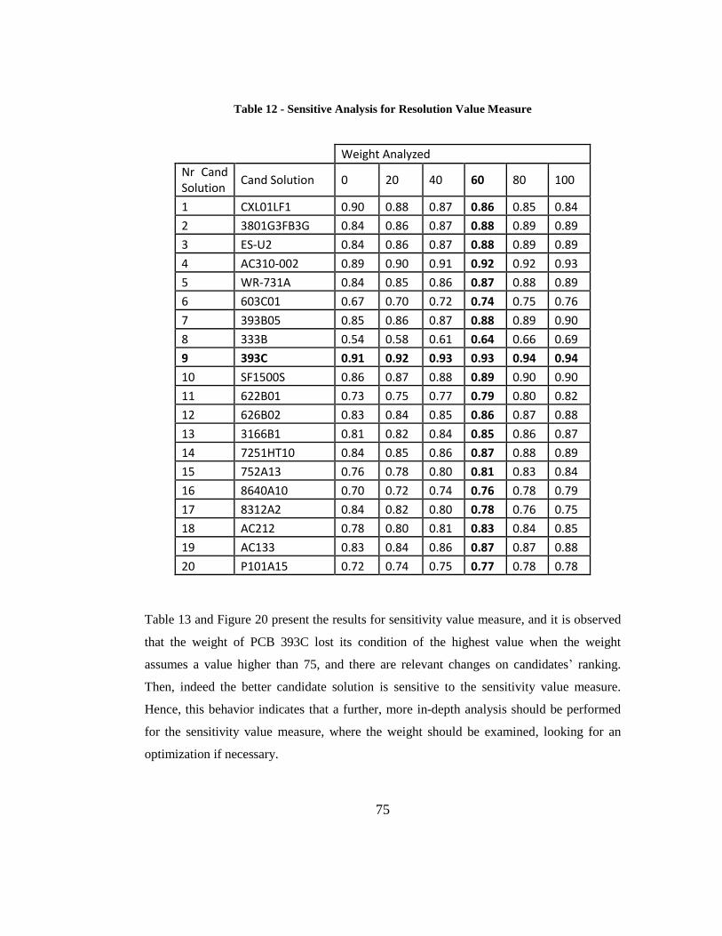
75
Table 12 - Sensitive Analysis for Resolution Value Measure
Weight Analyzed
Nr Cand Solution
Cand Solution 0 20 40 60 80 100
1 CXL01LF1 0.90 0.88 0.87 0.86 0.85 0.84
2 3801G3FB3G 0.84 0.86 0.87 0.88 0.89 0.89
3 ES-U2 0.84 0.86 0.87 0.88 0.89 0.89
4 AC310-002 0.89 0.90 0.91 0.92 0.92 0.93
5 WR-731A 0.84 0.85 0.86 0.87 0.88 0.89
6 603C01 0.67 0.70 0.72 0.74 0.75 0.76
7 393B05 0.85 0.86 0.87 0.88 0.89 0.90
8 333B 0.54 0.58 0.61 0.64 0.66 0.69
9 393C 0.91 0.92 0.93 0.93 0.94 0.94
10 SF1500S 0.86 0.87 0.88 0.89 0.90 0.90
11 622B01 0.73 0.75 0.77 0.79 0.80 0.82
12 626B02 0.83 0.84 0.85 0.86 0.87 0.88
13 3166B1 0.81 0.82 0.84 0.85 0.86 0.87
14 7251HT10 0.84 0.85 0.86 0.87 0.88 0.89
15 752A13 0.76 0.78 0.80 0.81 0.83 0.84
16 8640A10 0.70 0.72 0.74 0.76 0.78 0.79
17 8312A2 0.84 0.82 0.80 0.78 0.76 0.75
18 AC212 0.78 0.80 0.81 0.83 0.84 0.85
19 AC133 0.83 0.84 0.86 0.87 0.87 0.88
20 P101A15 0.72 0.74 0.75 0.77 0.78 0.78
Table 13 and Figure 20 present the results for sensitivity value measure, and it is observed
that the weight of PCB 393C lost its condition of the highest value when the weight
assumes a value higher than 75, and there are relevant changes on candidates’ ranking.
Then, indeed the better candidate solution is sensitive to the sensitivity value measure.
Hence, this behavior indicates that a further, more in-depth analysis should be performed
for the sensitivity value measure, where the weight should be examined, looking for an
optimization if necessary.

76
Table 13 - Sensitive Analysis for Sensitivity Value Measure
Weight Analyzed
Nr Cand Solution
Cand Solution 0 10 30 50 90 100
1 CXL01LF1 0.86 0.86 0.86 0.86 0.86 0.86
2 3801G3FB3G 0.93 0.92 0.90 0.88 0.85 0.84
3 ES-U2 0.87 0.87 0.87 0.88 0.88 0.88
4 AC310-002 0.93 0.93 0.92 0.92 0.91 0.91
5 WR-731A 0.85 0.85 0.86 0.87 0.89 0.89
6 603C01 0.88 0.84 0.79 0.74 0.65 0.64
7 393B05 0.86 0.86 0.87 0.88 0.90 0.90
8 333B 0.76 0.73 0.68 0.64 0.57 0.56
9 393C 1.00 0.98 0.96 0.93 0.89 0.89
10 SF1500S 0.93 0.92 0.91 0.89 0.87 0.86
11 622B01 0.94 0.91 0.84 0.79 0.70 0.68
12 626B02 0.97 0.94 0.90 0.86 0.80 0.79
13 3166B1 0.95 0.93 0.88 0.85 0.79 0.78
14 7251HT10 0.98 0.95 0.91 0.87 0.81 0.80
15 752A13 0.85 0.84 0.83 0.81 0.79 0.78
16 8640A10 0.84 0.82 0.79 0.76 0.71 0.70
17 8312A2 0.81 0.80 0.79 0.78 0.76 0.76
18 AC212 0.96 0.93 0.87 0.83 0.75 0.73
19 AC133 0.97 0.95 0.90 0.87 0.81 0.79
20 P101A15 0.91 0.88 0.82 0.77 0.68 0.66
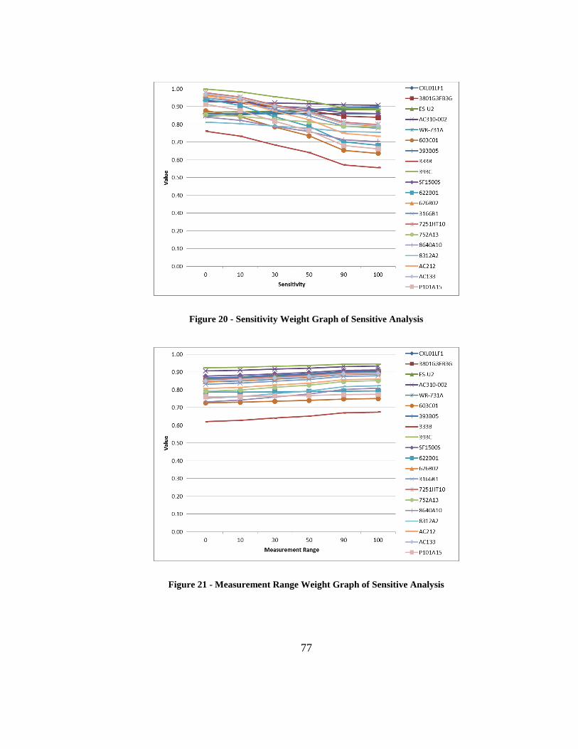
77
Figure 20 - Sensitivity Weight Graph of Sensitive Analysis
Figure 21 - Measurement Range Weight Graph of Sensitive Analysis

78
The results for measurement range value measure, depicted in Table 14 and Figure 21,
show a similar behavior of the candidate solutions observed on frequency and resolution
analysis, where the weight of PCB 393C also was the highest value after the weight
swinging process. Therefore, for the weight assessment of the measurement range value
measure, the better candidate solution is not sensitive to the weight, and there are no
relevant changes in the candidate solutions ranking which means that, a priori, no further
analysis of the weight will be necessary.
Table 14 - Sensitive Analysis for Measurement Range Value Measure
Weight Analyzed
Nr Cand Solution
Cand Solution 0 10 30 50 90 100
1 CXL01LF1 0.84 0.85 0.86 0.87 0.89 0.89
2 3801G3FB3G 0.86 0.87 0.88 0.89 0.90 0.90
3 ES-U2 0.86 0.87 0.88 0.89 0.90 0.90
4 AC310-002 0.91 0.91 0.92 0.92 0.93 0.93
5 WR-731A 0.86 0.86 0.87 0.88 0.90 0.90
6 603C01 0.73 0.73 0.74 0.74 0.75 0.75
7 393B05 0.87 0.87 0.88 0.89 0.90 0.91
8 333B 0.62 0.63 0.64 0.65 0.67 0.67
9 393C 0.92 0.93 0.93 0.94 0.94 0.95
10 SF1500S 0.88 0.88 0.89 0.90 0.91 0.91
11 622B01 0.79 0.79 0.79 0.79 0.79 0.79
12 626B02 0.85 0.85 0.86 0.87 0.89 0.89
13 3166B1 0.83 0.84 0.85 0.86 0.88 0.88
14 7251HT10 0.86 0.86 0.87 0.88 0.90 0.90
15 752A13 0.79 0.80 0.81 0.83 0.85 0.85
16 8640A10 0.73 0.74 0.76 0.78 0.80 0.81
17 8312A2 0.75 0.76 0.78 0.79 0.82 0.82
18 AC212 0.81 0.81 0.83 0.84 0.86 0.86
19 AC133 0.85 0.86 0.87 0.87 0.89 0.89
20 P101A15 0.76 0.76 0.77 0.77 0.77 0.77

79
Figure 22 - Operating Temperature Range Weight Graph of Sensitive Analysis
On the last sensitive analysis, Table 15 and Figure 22 detail the results for operating
temperature value measure. As observed in the sensitivity value measure, the weight of
PCB 393C lost its condition of the highest value when the weight assumes a value lower
than 30, and this behavior is observed intensively in other candidate solutions with relevant
changes on candidates’ ranking. Indeed, it is noticeable that better candidate solution is
sensitive to the operating temperature value measure. In consequence, this indicates that it
will be necessary to perform a further analysis for this value measure, where the weight
should be analyzed as necessary.
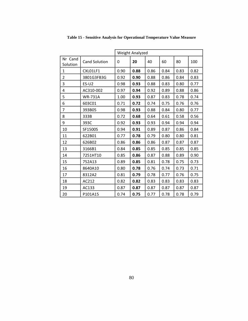
80
Table 15 - Sensitive Analysis for Operational Temperature Value Measure
Weight Analyzed
Nr Cand Solution
Cand Solution 0 20 40 60 80 100
1 CXL01LF1 0.90 0.88 0.86 0.84 0.83 0.82
2 3801G3FB3G 0.92 0.90 0.88 0.86 0.84 0.83
3 ES-U2 0.98 0.93 0.88 0.83 0.80 0.77
4 AC310-002 0.97 0.94 0.92 0.89 0.88 0.86
5 WR-731A 1.00 0.93 0.87 0.83 0.78 0.74
6 603C01 0.71 0.72 0.74 0.75 0.76 0.76
7 393B05 0.98 0.93 0.88 0.84 0.80 0.77
8 333B 0.72 0.68 0.64 0.61 0.58 0.56
9 393C 0.92 0.93 0.93 0.94 0.94 0.94
10 SF1500S 0.94 0.91 0.89 0.87 0.86 0.84
11 622B01 0.77 0.78 0.79 0.80 0.80 0.81
12 626B02 0.86 0.86 0.86 0.87 0.87 0.87
13 3166B1 0.84 0.85 0.85 0.85 0.85 0.85
14 7251HT10 0.85 0.86 0.87 0.88 0.89 0.90
15 752A13 0.89 0.85 0.81 0.78 0.75 0.73
16 8640A10 0.80 0.78 0.76 0.74 0.73 0.71
17 8312A2 0.81 0.79 0.78 0.77 0.76 0.75
18 AC212 0.82 0.82 0.83 0.83 0.83 0.83
19 AC133 0.87 0.87 0.87 0.87 0.87 0.87
20 P101A15 0.74 0.75 0.77 0.78 0.78 0.79

81
Chapter 5 CONCLUSIONS
5.1. Summary of Work and Results
With the constant aging process of bridges due to environmental conditions and
operational loads, the nation’s transportation agencies are in need of novel approaches to
help improve public safety. There are many bridges in the US that present relevant risk of
failure, according the ASCE 2013 report, but this number is decreasing due the effort on
bridge inspection and monitoring systems. Bridge SHM systems have helped to improve
structural monitoring to provide decision makers with reliable information regarding the
health of these structures. The field of SHM has been researched and new methodologies
and technologies have been proposed, contributing to its development, but there are still
many improvement opportunities that require research efforts by academia and industry
practitioners.
This thesis work described the results from a literature review effort to understand the
state-of-the-art related to SHM systems for bridge inspections. The review discussed the
types of monitoring based on a time frame and the scale of monitoring, and it presented the
methodologies of damage detection used on bridges monitoring and inspections. Non-
destructive tests are largely applied in bridge inspection traditional procedures, and the
vibration-based methods and pattern recognition methods are used on SHM systems. The
main concepts and theory behind these methods are thoroughly explained to clarify their
applicability, drawbacks, and limitations. The main components of the SHM system which
were identified in literature are described and analyzed to understand the function of each
in the system. This review was finalized with the presentation of most common sensors
applied in bridge monitoring. They are part of the sensory system and are responsible for

82
reading the environmental phenomena which act on the bridge, thereby obtaining the
required data of the structural health to be analyzed. Also, presented were their
technological concepts, applicability, drawbacks, and limitations that characterize each
type of sensor. This overall review was designed to provide a general knowledge of the
bridge structural monitoring field, highlighting the main features that will be applied to
achieve the main objective of this thesis and in further research.
The second objective of this thesis was to present a detailed study of value modeling
methodology, which is applied in system engineering to assess systems and components in
order to provide more qualified resources for decision makers to make a more logical and
defensible decision. Presented herein are the steps of methodology, showing the
components which were defined to allow the application of value modeling approach,
which has two distinctive models: the qualitative and quantitative. The qualitative value
model defined the hierarchy structure of the value model for the component under
assessment, observing the completeness, the mutuality exclusive, operability, and smallest
size for the model and objectives. This model defined the fundamental objective, identified
the functions that provide value, identified the objectives and the value measures. The
quantitative value model described a thorough analysis of all the resources available for the
model to ensure reliable results could be found with the calculation. The main outcomes of
the quantitative model were the value function and the swing weight matrix, and the
mathematical relation involving both factors resulted in the value attributed to candidate
solution.
The last part of the thesis applied the value based methodology to classify the candidate
solutions proposed in a list of accelerometers. These vibration sensors were selected from
research papers which analyzed bridge SHM systems and described the type of sensor it
employed. To complete the list researches was done on sensor manufacturers, and there
were added to list of sensors with features meeting the bridge monitoring demands. The
application of the methodology yielded a rank list of the candidate solutions, which was
submitted to a sensitive analysis to assure the reliability of the results. The sensitive
analysis indicated that the best evaluated candidate solution was not sensitive for three

83
weights, but it was sensitive for other two weights, indicating the necessity of further
analysis for these two weights. Thus, the main conclusions of this sensitive analysis were
compelling, so that the best candidate solution was confirmed as the better solution under
the analyzed objectives. In conclusion, a list of the key results of this study is provided
below.
- The value modeling methodology provides an efficient tool to score holistically the
candidate solutions with each of the n value measures.
- The development of the value functions can be simple and done fast, and this
feature makes it a good tool to be used by systems engineers to develop a reliable
candidate solutions ranking.
- The major advantage of the value modeling approach is that it provides assurance
for identifying the highest value candidate solution possible, given the selected
objectives after qualitative analysis.
5.2. Future Researches
SHM offers many opportunities for further research, but from the research stemming from
the presented thesis there are some especially interesting possible further research areas.
The value function can be analyzed to understand better what would be the most effective
range of a value measure to assure a flatter curve. Also, the expansion of the methodology
to be applied in the whole monitoring system helping to identify most adequate
components for the system. A further investigation to understand the weight behavior and
its impact on the best candidate solution rank is needed because of the swinging weight
process on sensitive analysis. Hence, these are some directions that research could follow
from this paper, and the author wishes to have motivated new investigations based on the
presented work.
84
REFERENCES
[1] D. Agdas, J. A. Rice, J. R. Martinez, and I. R. Lasa, “Comparison of Visual
Inspection and Structural-Health Monitoring As Bridge Condition Assessment
Methods,” J. Perform. Constr. Facil., vol. 26, no. 4, pp. 371–376, 2012.
[2] E. J. Cross, K. Worden, and C. R. Farrar, “Structural health monitoring for civil
infrastructure,” in Health Assessment of Engineered Structures. Bridges, Buildings
and Other Infrastructures, A. Haldar, Ed. Singapore: World Scientific Publishing,
2013, pp. 1–32.
[3] D. Huston, Structural Sensing, Health Monitoring, and Performance Evaluation
(Series in Sensors). Boca Raton: Taylor & Francis - CRC Press, 2011.
[4] F. N. Catbas, M. Susoy, and D. M. Frangopol, “Structural health monitoring and
reliability estimation: Long span truss bridge application with environmental
monitoring data,” Eng. Struct., vol. 30, no. 9, pp. 2347–2359, 2008.
[5] W. Chen and L. Duan, Handbook of International Bridge Engineering. Boca Raton:
CRC Press, 2014.
[6] T. W. Ryan, J. EricMann, Z. M. Chill, and B. T. Ott, “Bridge Inspector’s Reference
Manual,” 2012.
[7] S. B. Chase, “The role of sensing and measurement in achieving FHWA’S strategic
vision for highway infrastructure,” in Sensing Issues in Civil Structural Health
Monitoring, F. Ansari, Ed. Dordrecht: Springer, 2005, pp. 23–32.
[8] Y.-L. Xu and Y. Xia, Structural Health Monitoring of Long-span Suspension
Bridges. New York: Spon Press, 2012.
[9] A. Gastineau, T. Johnson, and A. Schultz, “Bridge Health Monitoring and
Inspections–A Survey of Methods,” Minneapolis, 2009.
[10] “ASCE 2013 Report Card for America’s Infrastructure.”
[11] N. G. Shrive, “Intelligent Structural Health Monitoring: a Civil Engineering
Perspective,” EEE Int. Conf. Syst. Man Cybern., pp. 1973–1977, 2005.

85
[12] B. Chen, X. Wang, D. Sun, and X. Xie, “Integrated system of structural health
monitoring and intelligent management for a cable-stayed bridge,” Sci. World J.,
vol. 2014, 2014.
[13] A. Plankis, “STRUCTURAL HEALTH MONITORING MEMS SENSORS
USING ELASTICITY-BASED BEAM VIBRATIONS,” Colorado State
University, 2012.
[14] V. M. Karbhari and F. Ansari, Eds., Structural Health Monitoring of Civil
Infrastructure Systems. Cambridge: Woodhead Publishing Limited, 2009.
[15] A. Zarafshan, A. Iranmanesh, and F. Ansari, “Vibration-Based Method and Sensor
for Monitoring of Bridge Scour,” J. Bridg. Eng., vol. 17, no. 6, pp. 829–838, 2012.
[16] A. Pyayt, A. Kozionov, I. Mokhov, B. Lang, R. Meijer, V. Krzhizhanovskaya, and
P. Sloot, “Time-Frequency Methods for Structural Health Monitoring,” Sensors,
vol. 14, pp. 5147–5173, 2014.
[17] B. J. A. Costa and J. A. Figueiras, “Fiber optic based monitoring system applied to
a centenary metallic arch bridge: Design and installation,” Eng. Struct., vol. 44, pp.
271–280, 2012.
[18] K. Worden, “Structural Health Monitoring using Pattern Recognition,” in New
Trends in Vibration Based Structural Health Monitoring, A. Deraemaeker and K.
Worden, Eds. Udine - Italy: SpringerWienNewYork, 2010, pp. 183–246.
[19] Y. Dong, R. Song, and H. Liu, “Bridges Structural Health Monitoring and
Deterioration Detection-Synthesis of Knowledge and Technology,” 2010.
[20] J. M. Ko and Y. Q. Ni, “Technology developments in structural health monitoring
of large-scale bridges,” Eng. Struct., vol. 27, no. 12 SPEC. ISS., pp. 1715–1725,
2005.
[21] K. Worden and G. Manson, “The application of machine learning to structural
health monitoring,” Philos. Trans. R. Soc. A Math. Phys. Eng. Sci., vol. 365, no.
1851, pp. 515–537, 2007.
[22] Y.-L. Xu and Y. Xia, “Structural Damage Detection,” in Structural Health
Monitoring of Long-span Suspension Bridges, New York - USA: Spon Press, 2012,
pp. 282–309.
[23] F. Magalhães, A. Cunha, and E. Caetano, “Vibration based structural health
monitoring of an arch bridge: From automated OMA to damage detection,” Mech.
Syst. Signal Process., vol. 28, pp. 212–228, 2012.

86
[24] A. Rytter, “Vibrational Based Inspection of Civil Engineering Structures,” Dept. of
Building Technology and Structural Engineering, Aalborg, 1993.
[25] C.-P. Fritzen, M. Klinkov, and P. Kraemer, “Vibration-Based Damage Diagnosis
and Monitoring of External Loads,” in New Trends in Structural Health
Monitoring, vol. 542, W. Ostachowicz and J. A. Güemes, Eds. Udine - Italy:
Springer, 2013, p. 432.
[26] L. Bisby and M. B. Briglio, “An Introduction to Structural Health Monitoring,”
ISIS Canada, 2006.
[27] A. Haldar, Ed., Health assessment of engineered structures : bridges, buildings, and
other infrastructures. Singapore: World Scientific Publishing, 2013.
[28] D. Balageas, C.-P. Fritzen, and A. Güemes, Structural Health Monitoring. Newport
Beach, USA: ISTE Ltd, 2006.
[29] C. Boller, F. Chang, and Y. Fujino, Eds., Encyclopedia of Structural Health
Monitoring. Chichester - UK: John Wiley & Sons, 2009.
[30] C. R. Farrar and K. Worden, Structural Health Monitoring a Machine Learning
Perspective. Chichester - UK: John Wiley & Sons, Ltd, 2013.
[31] H. Wenzel, Health Monitoring of Bridges. West Sussex-UK: John Wiley & Sons,
Ltd, 2009.
[32] J. Collins, G. Mullins, C. Lewis, and D. Winters, “State of the Practice and Art for
Structural Health Monitoring of Bridge Substructures,” 2014.
[33] M. L. Wang, J. P. Lynch, and H. Sohn, Eds., Sensor Technologies for Civil
Infrastructures, vol. 1. Woodhead Publishing, 2014.
[34] H. Xu and J. Humar, “Damage detection in a girder bridge by artificial neural
network technique,” Comput. Civ. Infrastruct. Eng., vol. 21, no. 6, pp. 450–464,
2006.
[35] S. W. Doebling, C. R. Farrar, and M. B. Prime, “A Summary Review of Vibration-
Based Damage Identification Methods,” Shock Vib. Dig., vol. 30, no. 2, pp. 91–105,
1998.
[36] S. Kashif Ur Rehman, Z. Ibrahim, S. A. Memon, and M. Jameel, “Nondestructive
test methods for concrete bridges: A review,” Constr. Build. Mater., vol. 107, pp.
58–86, 2016.

87
[37] R. L. Crane and J. S. Knopp, “Nondestructive inspection,” in Handbook of
Measurement in Science and Engineering, vol. 2, M. Kutz, Ed. John Wiley & Sons,
2013, pp. 1343–1411.
[38] M. Enckell, J. Egede Andersen, B. Glisic, J. Silfwerbrand, and M. Kutz, “New and
Emerging Technologies in Structural Health Monitoring,” in Handbook of
Measurement in Science and Engineering, vol. 1, M. Kutz, Ed. John Wiley & Sons,
2013, pp. 3–78.
[39] W. R. Wickramasinghe, D. P. Thambiratnam, T. H. T. Chan, and T. Nguyen,
“Vibration characteristics and damage detection in a suspension bridge,” J. Sound
Vib., vol. 375, no. 4, pp. 254–274, May 2016.
[40] V. M. Karbhari and L. S.-W. Lee, “Vibration-based damage detection techniques
for structural health monitoring of civil infrastructure systems,” in Structural health
monitoring of civil infrastructure systems, V. M. Karbhari and F. Ansari, Eds.
Cambridge: Woodhead Publishing Limited, 2009, pp. 177–212.
[41] P. Beena and R. Ganguli, “Structural damage detection using fuzzy cognitive maps
and Hebbian learning,” Appl. Soft Comput., vol. 11, no. 1, pp. 1014–1020, 2011.
[42] K. Smarsly and D. Hartmann, “Artificial Intelligence in Structural Health
Monitoring,” in The Third International Conference on Structural Engineering,
Mechanics and Computation. Cape Town, South Africa, 2007, pp. 705–710.
[43] M. Awad and R. Khanna, Efficient learning machines: Theories, concepts, and
applications for engineers and system designers. Apress, 2015.
[44] A. E. Aktan, F. N. Catbas, K. A. Grimmelsman, and M. Pervizpour, “Development
of a model health monitoring guide for major bridges,” 2003.
[45] M. Kutz, Ed., Handbook of Measurement in Science and Engineering, vol. 1. John
Wiley & Sons, 2013.
[46] M. J. Whelan, M. V. Gangone, K. D. Janoyan, and R. Jha, “Real-time wireless
vibration monitoring for operational modal analysis of an integral abutment
highway bridge,” Eng. Struct., vol. 31, no. 10, pp. 2224–2235, 2009.
[47] M. Modares and J. Mohammadi, “Sensors Used in Structural Health Monitoring,”
in Health assessment of engineered structures : bridges, buildings, and other
infrastructures, A. Haldar, Ed. Singapore: World Scientific Publishing, 2013, pp.
295–309.
[48] W. F. Ranson and R. I. Vachon, “Operational Loads Sensors,” in Encyclopedia of
Structural Health Monitoring, C. Boller, F.-K. Chang, and Y. Fujino, Eds.
Chichester - UK: John Wiley & Sons, 2009, pp. 993–1002.

88
[49] C. Aszkler, “Acceleration, Shock and Vibration Sensors,” in Sensor Technology
Handbook, J. S. Wilson, Ed. Oxford: Elsevier, 2005, pp. 137–154.
[50] A. Deraemaeker, “Vibration based structural health monitoring using large sensor
arrays: overview of instrumentation and feature extraction based on modal filters,”
in New Trends in Vibration Based Structural Health Monitoring, A. Deraemaeker
and K. Worden, Eds. Udine - Italy: SpringerWienNewYork, 2010, pp. 19–54.
[51] M. Tuttle, “Resistive strain measurement devices,” in Handbook of Measurement in
Science and Engineering, vol. 1, M. Kutz, Ed. John Wiley & Sons, 2013, pp. 659–
681.
[52] E. V. Monzon, A. M. Itani, and G. Pekcan, “Seismic testing of highway bridges,” in
Handbook of Measurement in Science and Engineering, vol. 1, M. Kutz, Ed. John
Wiley & Sons, 2013, pp. 133–158.
[53] M. Modares and N. Waksmanski, “Overview of Structural Health Monitoring for
Steel Bridges,” Pract. Period. Struct. Des. Constr., vol. 18, no. 3, pp. 187–191,
2013.
[54] M. L. Wang, J. P. Lynch, and H. Sohn, Eds., Sensor Technologies for Civil
Infrastructures, vol. 2. Cambridge: Woodhead Publishing, 2014.
[55] D. Ozevin, “Micro-electro-mechanical-systems (MEMS) for assessing and
monitoring civil infrastructures,” in Sensor Technologies for Civil Infrastructures,
vol. 1, M. L. Wang, J. P. Lynch, and H. Sohn, Eds. Cambridge: Woodhead
Publishing, 2014, pp. 265 – 294.
[56] M. J. Kwinn, G. S. Parnell, and R. A. Dees, “Decision making,” in Decision
Making in Systems Engineering and Management, Second., G. S. Parnell, P. J.
Driscoll, and D. L. Henderson, Eds. Hoboken: John Wiley & Sons, 2011, pp. 395–
446.
[57] R. L. Keeney, Value-focused thinking: A Path to Creative Decisionmaking.
Cambridge: Harvard University Press, 1992.
[58] G. S. Parnell and P. D. West, “Systems Decision Process Overview,” in Decision
Making in Systems Engineering and Management, Second., G. S. Parnell, P. J.
Driscoll, and D. L. Henderson, Eds. Hoboken: John Wiley & Sons, 2011, pp. 275–
295.
[59] T. Trainor and G. S. Parnell, “Problem definition,” in Decision Making in Systems
Engineering and Management, Second., G. S. Parnell, P. J. Driscoll, and D. L.
Henderson, Eds. Hoboken: John Wiley & Sons, 2011, pp. 297–352.

89
[60] “Accelerometer Terminology Guide,” Denver, 2007.
[61] M. Fraser, A. Elgamal, X. He, and J. P. Conte, “Sensor Network for Structural
Health Monitoring of a Highway Bridge,” J. Comput. Civ. Eng., vol. 24, no.
January/February, pp. 11–24, 2010.
[62] J. M. W. Brownjohn, F. Magalhães, E. Caetano, and A. Cunha, “Ambient vibration
re-testing and operational modal analysis of the Humber Bridge,” Eng. Struct., vol.
32, no. 8, pp. 2003–2018, 2010.
[63] S. Dahal, “Structural Health Monitoring for In-Service Highway Bridges Using
Smart Sensors Structural Health Monitoring for In-Service Highway,” 2013.
[64] C. Gentile and A. Saisi, “Ambient vibration testing and condition assessment of the
Paderno iron arch bridge (1889),” Constr. Build. Mater., vol. 25, no. 9, pp. 3709–
3720, 2011.
[65] D. M. Siringoringo and Y. Fujino, “System identification of suspension bridge from
ambient vibration response,” Eng. Struct., vol. 30, no. 2, pp. 462–477, 2008.
[66] F. Magalhães, A. Cunha, and E. Caetano, “Dynamic monitoring of a long span arch
bridge,” Eng. Struct., vol. 30, no. 11, pp. 3034–3044, 2008.
[67] E. R. Johnson, G. S. Parnell, and S. N. Tani, “Perform Deterministic Analysis and
Develop Insights,” in Handbook of Decision Analysis, G. S. Parnell, T. A. Bresnick,
S. N. Tani, and E. R. Johnson, Eds. Hoboken: John Wiley & Sons, 2013, pp. 166–
226.
[68] G. S. Parnell, “Value-Focused Thinking Using Multiple Objective Decision
Analysis,” in Methods for Conducting Military Operational Analysis: Best
Practices in Use Throughout the Department of Defense, A. Loerch and L. Rainey,
Eds. Military Operations Research Society, 2007.
[69] C. W. Kirkwood, Strategic Decision Making: Multiobjective Decision Analysis with
Spreadsheets. Belmont: Duxbury Press, 1997.
[70] C. W. Kirkwood, “Decision Analysis,” in Handbook of Systems Engineering and
Management, Secong., A. P. Sage and W. B. Rouse, Eds. Hoboken: John Wiley &
Sons, 2014, pp. 1223–1250.
[71] M. J. Chae, H. S. Yoo, J. Y. Kim, and M. Y. Cho, “Development of a wireless
sensor network system for suspension bridge health monitoring,” Autom. Constr.,
vol. 21, no. 1, pp. 237–252, 2012.

90
[72] F. N. Catbas, M. Gul, R. Zaurin, H. B. Gokce, T. Terrell, T. Dumlupinar, and D.
Maier, “Long term bridge maintenance monitoring demonstration on a movable
bridge,” Orlando, 2010.
[73] K. Maes, J. Peeters, E. Reynders, G. Lombaert, and G. De Roeck, “Identification of
axial forces in beam members by local vibration measurements,” J. Sound Vib., vol.
332, no. 21, pp. 5417–5432, Oct. 2013.
[74] W. H. Hu, E. Caetano, and A. Cunha, “Structural health monitoring of a stress-
ribbon footbridge,” Eng. Struct., vol. 57, pp. 578–593, 2013.
[75] L. Lorieux, “Analysis of train-induced vibrations on a single-span composite
bridge,” Royal Institute of Technology (KTH), 2008.