VALLIAMMAI ENGINEERING COLLEGE Semester/EE6511...2. (a)Maxwell s Bridge (b) Schering Bridge 3. (a)...
132
VALLIAMMAI ENGINEERING COLLEGE SRM Nagar, Kattankulathur – 603 203 DEPARTMENT OF ELECTRICAL AND ELECTRONICS ENGINEERING EE6511 CONTROL AND INSTRUMENTATION LABORATORY MANUAL 2017-2018 ODD SEMESTER Prepared by, Dr.R.Arivalahan/Asso.Prof. Mr.S.Padhmanabha Iyappan/AP-Sr.G Ms.P.Bency/AP-O.G Ms.R.V.Preetha/AP-O.G Ms.G.Shanthi/AP-O.G
Transcript of VALLIAMMAI ENGINEERING COLLEGE Semester/EE6511...2. (a)Maxwell s Bridge (b) Schering Bridge 3. (a)...

VALLIAMMAI ENGINEERING COLLEGE
SRM Nagar, Kattankulathur – 603 203
DEPARTMENT OF ELECTRICAL AND ELECTRONICS ENGINEERING
EE6511 CONTROL AND INSTRUMENTATION LABORATORY MANUAL
2017-2018 ODD SEMESTER
Prepared by,
Dr.R.Arivalahan/Asso.Prof.
Mr.S.Padhmanabha Iyappan/AP-Sr.G
Ms.P.Bency/AP-O.G
Ms.R.V.Preetha/AP-O.G
Ms.G.Shanthi/AP-O.G

EE6511 Control and Instrumentation Lab Department of EEE 2017 - 2018
INDEX
Sl.
No.
Date of
Expt. Name of the Experiment
Page
No. Marks
Staff sign.
with date
1.
2.
3.
4.
5.
6.
7.
8.
9.
10.
11.
12.
13.
14.
15.

EE6511 Control and Instrumentation Lab Department of EEE 2017 - 2018
EE6511 CONTROL AND INSTRUMENTATION LAB
SYLLABUS
CONTROL SYSTEMS
1. P, PI and PID controllers
2. Stability Analysis
3. Modeling of Systems – Machines, Sensors and Transducers
4. Design of Lag, Lead and Lag-Lead Compensators
5. Position Control Systems
6. Synchro-Transmitter- Receiver and Characteristics
7. Simulation of Control Systems by Mathematical development tools.
INSTRUMENTATION
8. Bridge Networks –AC and DC Bridges
9. Dynamics of Sensors/Transducers a. Temperature b. Pressure c. Displacement
d. Optical e. Strain f. Flow
10. Power and Energy Measurement
11. Signal Conditioning
a. Instrumentation Amplifier
b. Analog – Digital and Digital –Analog converters (ADC and DACs)
12. Process Simulation.
BEYOND THE SYLLABUS EXPERIMENTS
1. Determination of transfer function of AC Servomotor
2. Measurement of Inductance using Anderson Bridge

EE6511 Control and Instrumentation Lab Department of EEE 2017 - 2018
CYCLE I
1. (a) Wheatstone Bridge (b) Kelvin’s Double Bridge
2. (a)Maxwell’s Bridge
(b) Schering Bridge
3. (a) Study of Displacement Transducer – LVDT (b) Study of Pressure Transducer – Bourdon Tube 4. Calibration of Single Phase Energy Meter
5. (a) Calibration of Wattmeter
(b) Design of Instrumentation Amplifier
6. (a)Analog – Digital converters (b)Digital –Analog Converters
7. (a) Determination of Transfer Function of DC generator (b) Determination of Transfer Function of DC motor
CYCLE II
8. (a) DC Position Control System (b) AC Position Control System
9. Design of Lag, Lead and Lag-Lead Compensators
10. (a) Simulation of Control Systems by Mathematical development tools (b) Stability Analysis
11. Process Simulation
12. Time Domain and Frequency Domain Specifications 13. P, PI and PID controllers 14. Synchro-Transmitter- Receiver and Characteristics Additional Experiments
1. Analog simulation of Type – 0 and Type – 1 Systems
2. Determination of transfer function of AC Servomator

EE6511 Control and Instrumentation Lab Department of EEE 2017 - 2018
CIRCUIT DIAGRAM

EE6511 Control and Instrumentation Lab Department of EEE 2017 - 2018
Ex. No:
Date:
1(a).WHEATSTONE BRIDGE
AIM:
To measure the given medium resistance using Wheatstone bridge.
APPARATUS REQUIRED:
S.No Name of the Trainer Kit/
Components
Quantity
1. Wheatstone bridge trainer 1 2. Unknown Resistors specimen 5 different values 3. Connecting wires Few 4. DMM 1 5. CRO 1
THEORY:
Wheatstone bridge trainer consists of basic bridge circuit as screen printed on front panel
with a built in 1 kHz oscillator and an isolation transformer. The arm AC and AD consists of a
1K resistor. Arms BD consists of variable resistor. The unknown resistor (Rx) whose value is
to be determined is connected across the terminal BC .The resistor R2 is varied suitably to obtain
the bridge balance condition. The DMM is used to determine the balanced output voltage of the
bridge circuit.
For bridge balance,
For the galvanometer current to be zero the following conditions also exists
x
xRR
EII
11 and
E = EMF of the supply, combining the above equations we obtain
The unknown resistance. If three of the resistances are known, the fourth may be
determined.
PROCEDURE:
1. Connect the unknown resistor in the arm marked Rx. 2. Connect the DMM across the terminal CD and switch on the trainer kit. 3. Vary R2 to obtain the bridge balance condition. 4. Find the value of the unknown resistance Rx using DMM after removing wires. 5. Compare the practical value with the theoretical value of unknown resistance Rx calculated
using the formula.

EE6511 Control and Instrumentation Lab Department of EEE 2017 - 2018
PANEL DIAGRAM
TABULATION:
Sl.No R1 (Ω) R2 (Ω ) R3 (Ω ) Rx(Ω ) (Actual)
Rx(Ω ) (Observed)
Percentage
Error
1
2
3
4
5

EE6511 Control and Instrumentation Lab Department of EEE 2017 - 2018
MODEL CALCULATION:
RESULT:
Review Questions
1. What are the applications of Wheatstone bridge? 2. What are standard arm and ratio arm in Wheatstone bridge? 3. What are the detectors used for DC Bridge? 4. What do you meant by sensitivity? 5. Why Wheatstone bridge cannot be used to measure low resistances?

EE6511 Control and Instrumentation Lab Department of EEE 2017 - 2018
CIRCUIT DIAGRAM

EE6511 Control and Instrumentation Lab Department of EEE 2017 - 2018
Ex. No:
Date:
1(b). KELVIN’S DOUBLE BRIDGE
AIM:
To measure the given low resistance using Kelvin’s Double bridge.
APPARATUS REQUIRED:
THEORY:
Kelvin’s double bridge is a modification of Wheatstone’s bridge and provides more
accuracy in measurement of low resistances It incorporates two sets of ratio arms and the use
of four terminal resistors for the low resistance arms, as shown in figure. Rx is the resistance
under test and S is the resistor of the same higher current rating than one under test. Two
resistances Rx and S are connected in series with a short link of as low value of resistance r as
possible. P, Q, p, q are four known non inductive resistances, one pair of each (P and p, Q and q)
are variable. A sensitive galvanometer G is connected across dividing points PQ and pq. . The
ratio P Q is kept the same as p q , these ratios have been varied until the galvanometer reads
zero.
Balance Equation: For zero balance condition,
rqp
rqp
qp
pRI
rqp
rqpSRI
QP
P If
q
p
Q
P Then unknown resistance
PROCEDURE:
1. Connect the unknown resistance Rx as marked on the trainer 2. Connect a galvanometer G externally as indicated on the trainer 3. Energize the trainer and check the power to be +5 V. 4. Select the values of P and Q such that P/Q = p/q = 500/50000 = 0.01 5. Adjust P1 for proper balance and then at balance, measure the value of P1.
S.No Name of the Trainer Kit/ Components Quantity
1. Kelvin’s Double bridge trainer kit 1 2. Unknown Resistors specimen 5 3. Connecting wires Few 4. Galvanometer 1

EE6511 Control and Instrumentation Lab Department of EEE 2017 - 2018
PANEL DIAGRAM
TABULATION:
Sl.No P () Q () P1() Rx()
(Actual)
Rx()
(Observed)
%
Error

EE6511 Control and Instrumentation Lab Department of EEE 2017 - 2018
MODEL CALCULATION:
RESULT:
REVIEW QUESTIONS
1. Name the bridge used for measuring very low resistance. 2. Classify the resistances according to the values. 3. Write the methods of measurements of low resistance 4. What is the use of lead resistor in kelvin’s Double bridge? 5. Why Kelvin’s double bridge is having two sets of ratio arms?

EE6511 Control and Instrumentation Lab Department of EEE 2017 - 2018
CIRCUIT DIAGRAM

EE6511 Control and Instrumentation Lab Department of EEE 2017 - 2018
Ex. No:
Date:
2(a). MAXWELL’S BRIDGE
AIM:
To measure the unknown inductance and Q factor of a given coil.
APPARATUS REQUIRED :
S.No Name of the Trainer Kit/ Components Quantity
1. Maxwell’s inductance- capacitance bridge trainer kit
1
2. Unknown inductance specimen 3 different values 3. Connecting wires Few 4. Head phone/ CRO 1
THEORY :
In this bridge, an inductance is measured by comparison with a standard variable capacitance. The connection at the balanced condition is given in the circuit diagram. Let L1 = Unknown Inductance. R1 = effective resistance of Inductor L1. R2, R3 and R4 = Known non-inductive resistances. C4 = Variable standard Capacitor. writing the equation for balance condition,
3244
411
1RR
RCj
RLjR
separating the real and imaginary terms, we have
Thus we have two variables R4 and C4 which appear in one of the two balance equations and hence the two equations are independent. The expression for Q factor is given by
441
1 RCR
LQ
FORMULA USED:
Phasor Diagram

EE6511 Control and Instrumentation Lab Department of EEE 2017 - 2018
PANEL DIAGRAM
Procedure:
1. Connections are made as per the circuit diagram. 2. Connect the unknown inductance in the arm marked Lx . 3. Switch on the trainer kit. 4. Observe the sine wave at secondary of isolation transformer on CRO. 5. Vary R4 and C4 from minimum position in the clockwise direction to obtain the bridge
balance condition. 6. Connect the CRO between ground and the output point to check the bridge balance.
TABULATION:
Sl.
No.
R1
(Ω) R3
(Ω) C
(µF)
Lx
(mH)
Actual
Lx
(mH)
Observed
Quality
factor
Q

EE6511 Control and Instrumentation Lab Department of EEE 2017 - 2018
MODEL CALCULATION:
RESULT:
REVIEW QUESTIONS
1. What are the sources of errors in AC bridges? 2. List the various detectors used for AC Bridges. 3. Define Q factor of an inductor. Write the equations for inductor Q factor with RL series and parallel equivalent circuits. 4. Why Maxwell's inductance bridge is suitable for medium Q coils? 5. State merits and limitations of Maxwell's bridge when used for measurement of unknown inductance.

EE6511 Control and Instrumentation Lab Department of EEE 2017 - 2018
CIRCUIT DIAGRAM:

EE6511 Control and Instrumentation Lab Department of EEE 2017 - 2018
Ex. No:
Date:
2(b). SCHERING BRIDGE
AIM:
To measure the value of unknown capacitance using Schering’s bridge & dissipation factor. APPARATUS REQUIRED:
S. No. Components / Equipments Quantity
1. Schering’s bridge trainer kit 1 2. Decade Conductance Box 1 3. Digital Multimeter 1 4. CRO 1 5. Connecting wires Few
THEORY:
In this bridge the arm BC consists of a parallel combination of resistor & a Capacitor and the arm AC contains capacitor. The arm BD consists of a set of resistors varying from 1 to 1 M. In the arm AD the unknown capacitance is connected. The bridge consists of a built in power supply, 1 kHz oscillator and a detector. BALANCE EQUATIONS:
Let C1=Capacitor whose capacitance is to be measured. R1= a series resistance representing the loss in the capacitor C1. C2= a standard capacitor. R3= a non-inductive resistance. C4= a variable capacitor. R4= a variable non-inductive resistance in parallel with variable capacitor C4.
At balance, Z1Z4=Z2Z3
41 3
1 4 4 2
31 4 4 4
1 2
3 3 4 441 4
1 2 2
1 1.
1
11
Rr R
jωC jωC R jωC
Rr R jωC R
jωC jωCR R R CjR
r R jωC ωC C
Equating the real and imaginary terms, we obtain

EE6511 Control and Instrumentation Lab Department of EEE 2017 - 2018
Two independent balance equations are obtained if C4 and R4 are chosen as the variable elements.
Dissipation Factor:
The dissipation factor of a series RC circuit is defined as a co-tangent of the phase angle and therefore by definition the dissipation factor is
3 42 41 1 1 4 4
3 2
tan .R CC R
D δ ωC r ω ωC RR C
FORMULAE USED:
ωC4R4 where C4=Cx & R4=Rx
PROCEDURE:
1. Switch on the trainer board and connect the unknown in the arm marked Cx. 2. Observe the sine wave at the output of oscillator and patch the circuit by using the wiring
diagram. 3. Observe the sine wave at secondary of isolation transformer on CRO. Select some value of
R3. 4. Connect the CRO between ground and the output point of imbalance amplifier. 5. Vary R4 (500 Ω potentiometer ) from minimum position in the clockwise direction. 6. If the selection of R3 is correct, the balance point (DC line) can be observed on CRO. (That is
at balance the output waveform comes to a minimum voltage for a particular value of R4 and then increases by varying R3 in the same clockwise direction). If that is not the case, select another value of R4.
7. Capacitor C2 is also varied for fine balance adjustment. The balance of the bridge can be observed by using loud speaker.
8. Tabulate the readings and calculate the unknown capacitance and dissipation factor.

EE6511 Control and Instrumentation Lab Department of EEE 2017 - 2018
TABULATION:
S.No. C2
(µF) R3() R4()
Cx(F)
Dissipation
factor (D1) True
value
Measured
Value
MODEL CALCULATION:
RESULT:
REVIEW QUESTIONS:
1. State the two conditions for balancing an AC bridge? 2. State the uses of Schering’s Bridge? 3. What do you mean by dissipation factor? 4. Give the relationship between Q and D. 5. Derive the balance equations.

EE6511 Control and Instrumentation Lab Department of EEE 2017 - 2018
SCHEMATIC DIAGRAM FOR DISPLACEMENT TRANSDUCER

EE6511 Control and Instrumentation Lab Department of EEE 2017 - 2018
Ex. No:
Date:
3 (a). STUDY OF DISPLACEMENT TRANSDUCER – LVDT
AIM:
To study the displacement transducer using LVDT and to obtain its characteristic
APPARATUS REQUIRED :
S.No Name of the Trainer Kit/ Copmponents Quantity
1. LVDT trainer kit containing the signal conditioning unit
1
2. LVDT calibration jig 1 3. Multi meter 1 4. Patch cards Few
THEORY:
LVDT is the most commonly and extensively used transducer, for linear displacement
measurement. The LVDT consists of three symmetrical spaced coils wound onto an insulated
bobbin.
A magnetic core, which moves through the bobbin without contact, provides a path for
the magnetic flux linkage between the coils. The position of the magnetic core controls the
mutual inductance between the primary coil and with the two outside or secondary coils. When
an AC excitation is applied to the primary coil, the voltage is induced in secondary coils that are
wired in a series opposing circuit. When the core is centred between two secondary coils, the
voltage induced in the secondary coils are equal, but out of phase by 180°. The voltage in the two
coils cancels and the output voltage will be zero.
CIRCUIT OPERATION:
The primary is supplied with an alternating voltage of amplitude between 5V to 25V with
a frequency of 50 cycles per sec to 20 K cycles per sec. The two secondary coils are identical &
for a centrally placed core the induced voltage in the secondaries Es1&Es2 are equal. The
secondaries are connected in phase opposition. Initially the net o/p is zero. When the
displacement is zero the core is centrally located. The output is linear with displacement over a
wide range but undergoes a phase shift of 180°. It occurs when the core passes through the zero
displacement position.

EE6511 Control and Instrumentation Lab Department of EEE 2017 - 2018
GENERALIZED DIAGRAM:
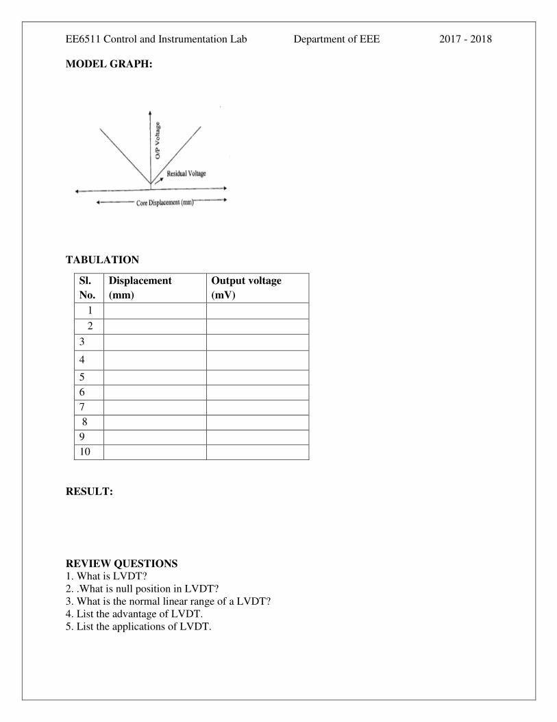
PROCEDURE:
1. Switch on the power supply to the trainer kit.
2. Rotate the screw gauge in clock wise direction till the voltmeter reads zero volts.
3. Rotate the screw gauge in steps of 2mm in clockwise direction and note down the o/p voltage.
4. Repeat the same by rotating the screw gauge in the anticlockwise direction from null position.
5. Plot the graph DC output voltage Vs Displacement
EE6511 Control and Instrumentation Lab Department of EEE 2017 - 2018
MODEL GRAPH:
TABULATION
RESULT:
REVIEW QUESTIONS
1. What is LVDT? 2. .What is null position in LVDT? 3. What is the normal linear range of a LVDT? 4. List the advantage of LVDT. 5. List the applications of LVDT.
Sl.
No.
Displacement
(mm)
Output voltage
(mV)
1
2
3
4
5
6
7
8
9
10

EE6511 Control and Instrumentation Lab Department of EEE 2017 - 2018
Ex. No:
Date:
3 (b). STUDY OF PRESSURE TRANSDUCER – BOURDON TUBE
AIM:
To study the pressure transducer using Bourdon tube and to obtain its characteristics.
APPARATUS REQUIRED :
S.No Name of the Trainer Kit/ Components Quantity
1. Bourdon pressure transducer trainer 1
2. Foot Pump 1
3. Multi meter 1
4. Patch cards Few
THEORY:
Pressure measurement is important not only in fluid mechanics but virtually in every branch of Engineering. The bourdon pressure transducer trainer is intended to study the characteristics of a pressure(P) to current (I) converter. This trainer basically consists of
1. Bourdon transmitter. 2. Pressure chamber with adjustable slow release valve. 3. Bourdon pressure gauge (mechanical) 4. (4- 20) mA Ammeters, both analog and digital.
The bourdon transmitter consists of a pressure gauge with an outside diameter of 160 mm including a built-in remote transmission system. Pressure chamber consists or a pressure tank with a provision to connect manual pressure foot pump, slow release valve for discharging the air from this pressure tank, connections to mechanical bourdon pressure gauge, and the connections for bourdon pressure transmitter. Bourdon pressure gauge is connected to pressure chamber. This gauge helps to identify to what extent this chamber is pressurized.
There are two numbers of 20 mA Ammeters. A digital meter is connected in parallel with analog meter terminals and the inputs for these are terminated at two terminals (+ ve and – ve). So positive terminal and negative terminal of bourdon tube is connected to, positive and negative terminals of the Ammeters.
PROCEDURE:
1. The foot pump is connected to the pressure chamber. 2. Switch on the bourdon transducer trainer. 3. Release the air release valve by rotating in the counter clockwise direction. 4. Record the pressure and Voltage. 5. Use the foot pump and slowly inflate the pressure chamber, so that the pressure in the
chamber increases gradually. 6. Tabulate the result. 7. Draw the graph. Input pressure Vs Output voltage.

EE6511 Control and Instrumentation Lab Department of EEE 2017 - 2018
DIAGRAM:
MODEL GRAPH
TABULATION
Sl.
No.
Input Pressure
(PSI)
Output Pressure
(Kg/ cm2)
Output Voltage
mV
1
2
3
4
5
6
7
8
9
10

EE6511 Control and Instrumentation Lab Department of EEE 2017 - 2018
RESULT:
REVIEW QUESTIONS
1. Define Transducer. What are active and passive transducers? 2. List any four pressure measuring transducers? 3. What is the advantage of pinion in bourdon tube? 4. Write the operational principle of bourdon tube. 5. State the advantages of bourdon tube over bellows & diaphragms.

EE6511 Control and Instrumentation Lab Department of EEE 2017 - 2018
CIRCUIT DIAGRAM

EE6511 Control and Instrumentation Lab Department of EEE 2017 - 2018
Ex.No:
Date :
4. CALIBRATION OF SINGLE PHASE ENERGY METER
AIM: To calibrate the given energy meter using a standard wattmeter and to obtain percentage
error.
APPARATUS REQUIRED:
S. No. Components / Equipments Specification Quantity
1. Energy Meter Single Phase 1
2. Standard Wattmeter 300V, 10A, UPF 1
3. Voltmeter (MI) 0-300V 1
4. Ammeter (MI) 0-10A 1
5. Lamp Load 230V, 3KW 4
THEORY:
The energy meter is an integrated type instrument where the speed of rotation of
aluminium disc is directly proportional to the amount of power consumed by the load and the no
of revs/min is proportional to the amount of energy consumed by the load. In energy meter the
angular displacement offered by the driving system is connected to the gearing arrangement to
provide the rotation of energy meter visually. The ratings associated with an energy meter are
1. Voltage Rating2. Current Rating3. Frequency Rating
4. Meter Constants.
Based on the amount of energy consumption, the driving system provides rotational
torque for the moving system which in turn activates the energy registering system for reading
the real energy consumption.The energy meter is operated based on induction principle in which
the eddy current produced by the induction of eddy emf in the portion of the aluminium disc
which creates the driving torque by the interaction of 2 eddy current fluxes.

EE6511 Control and Instrumentation Lab Department of EEE 2017 - 2018
PROCEDURE:
1. Connections are given as per the circuit diagram.
2. The DPST switch is closed to give the supply to the circuit.
3. The load is switched on.
4. Note down the ammeter, voltmeter & wattmeter reading .Also note down the time taken for 5
revolutions for the initial load.
5. The number of revolutions can be noted down by adapting the following procedure. When
the red indication mark on the aluminium disc of the meter passes, start to count the number
of revolutions made by the disc by using a stop watch and note it down.
Repeat the above steps (4) for different load currents by varying the load for the fixed number of
revolutions.
FORMULA USED:
100%
ValueTrue
lueMeasuredVaValueTrueError
TABULATION:
Voltmeter
Reading, V
(Volt)
Ammeter
Reading,
I
(Amp)
Wattmeter
Reading, W
(Watt)
Time
Period,
t (Sec)
No. of
revolution
s
Energy Meter
Reading (kwh) %
Error Measured True

EE6511 Control and Instrumentation Lab Department of EEE 2017 - 2018
MODEL GRAPH:
MODEL CALCULATION:
RESULT:
REVIEW QUESTIONS
1. What do you meant by calibration?
2. What is the need for lag adjustment devices in single phase energy meter?
3. How damping is provided in energy meter?
4. What is "Creep" in energy meter? What are the causes of creeping in an energy meter?
5. How is creep effect in energy meters avoided?

EE6511 Control and Instrumentation Lab Department of EEE 2017 - 2018
CIRCUIT DIAGRAM:

EE6511 Control and Instrumentation Lab Department of EEE 2017 - 2018
Ex.No.:
Date :
5(a) CALIBRATION OF WATTMETER
AIM:To calibrate the given Wattmeter by direct loading and obtain its percentage error.
APPARATUS REQUIRED:
S. No. Components / Equipments Specification Quantity
1. Wattmeter 300V, 10A, UPF 1
2. Voltmeter (MI) 0-300V 1
3. Ammeter (MI) 0-10A 1
4. Lamp Load 230V, 3KW 1
5. Connecting wires --- Few
THEORY:
In Electro Dynamometer wattmeter there are 2 coils connected in different circuits to
measure the power. The fixed coil or held coil is connected in series with the load and so carry
the current in the circuit. The moving coil is connected across the load and supply and carries
the current proportional to the voltage.
The various parts of the wattmeter are 1. Fixed coil and Moving coil 2.. Controlling springs and
Damping systems 3. Pointer Here a spring control is used for resetting the pointer to the initial
position after the de-excitation of the coil. The damping system is used to avoid the
overshooting of the coil and hence the pointer. A mirror type scale and knife edge pointer is
provided to remove errors due to parallax.

EE6511 Control and Instrumentation Lab Department of EEE 2017 - 2018
PROCEDURE:
1. Connections are given as per the circuit diagram.
2. Power supply is switched on and the load is turned on.
3. The value of the load current is adjusted to the desired value.
4. The readings of the voltmeter, ammeter& wattmeter are noted.
5. The procedure is repeated for different values of the load current and for each value of load
current all the meter readings are noted.
TABULATION
S.No
Voltmete
r
reading
(Volts)
Ammeter
Reading
(Amp)
Wattmeter Reading (Watt)
% Error Measured
True value
P = V*I
FORMULA USED:
100%
ValueTrue
lueMeasuredvaTruevalueError
MODEL GRAPH:

EE6511 Control and Instrumentation Lab Department of EEE 2017 - 2018
MODEL CALCULATION:
RESULT:
REVIEW QUESTIONS
1. What do you mean by calibration
2. What are the common errors in Wattmeter?
3. Can we Measure power using one Wattmeter in a 3-Phase supply?
4. How do we measure Reactive Power.?
5. How do you compensate Pressure coil in Wattmeter?

EE6511 Control and Instrumentation Lab Department of EEE 2017 - 2018
CIRCUIT DIAGRAM

EE6511 Control and Instrumentation Lab Department of EEE 2017 - 2018
Ex.No:
Date :
5(b) DESIGN OF INSTRUMENTATION AMPLIFIER
AIM:
To design an instrumentation amplifier APPARATUS REQUIRED:
S.No. Components Specification Quantity 1. Op-Amp IC 741 3 2. Resistor 1 KΩ 6 3. Regulated Power Supply (0-30)V 2 4. Decade Resistance Box - 1 5. Bread Board - 1 6. Connecting Wires - Few
THEORY:
In industrial and consumer applications, the physical quantities such as temperature,
pressure, humidity, light intensity, water flow etc is measured with the help of transducers. The
output of transducer has to be amplified using instrumentation so that it can drive the indicator or
display system. The important features of an instrumentation amplifier are 1) high accuracy 2)
high CMRR 3) high gain stability with low temperature coefficient 4) low dc offset 5) low output
impedance.
The circuit diagram shows a simplified differential instrumentation amplifier. A variable
resistor (DRB) is connected in one arm, which is assumed as a transducer in the experiment and
it is changed manually. The voltage follower circuit and a differential OP-AMP circuit are
connected as shown.
PROCEDURE:
1. Give the connections as per the circuit diagram.
2. Switch on the RPS
3. Set Rg, V1 and V2 to particular values
4. Repeat Step 3 for different values of Rg, V1 and V2
5. Calculate the theoretical output voltage using the given formula and compare with
practical value.

EE6511 Control and Instrumentation Lab Department of EEE 2017 - 2018
OBSERVATION:
S.No V1 V2 Vd= (V1-V2)
Volts
Vo
(Practical)
Gain A= Vout/
Vd
Vo
(Theoretical)
FORMULA:
d
g
VR
R
R
RV
21
1
20
Vo = A*Vd Where
AR
R
R
R
g
21
1
2

EE6511 Control and Instrumentation Lab Department of EEE 2017 - 2018
MODEL CALCULATIONS:
RESULT:
REVIEW QUESTIONS:
1. What is the difference between instrumentation amplifier and differential amplifier?
2. What are the characteristics of instrumentation amplifier?
3. What is CMRR?
4. What are the applications of instrumentation amplifier?
5. What is the other name of instrumentation amplifier?

EE6511 Control and Instrumentation Lab Department of EEE 2017 - 2018
CIRCUIT DIAGRAM :
3
2
7
4_
+
6
+15
-15
IC 741
7408
1.5K
6
Output
Reset( Logic 1
Analog Input ( -Ve ) 1
2
3
Ck
A B C D
14
121
9 8 112
310
R - 2R Ladder Type DAC
IC - 7493Binary Counter
For DAC R = 1.5K 2R = 3.3K Rf = 6.8K
)

EE6511 Control and Instrumentation Lab Department of EEE 2017 - 2018
Ex.No.
Date:
6(a) ANALOG – DIGITAL CONVERTER
AIM:
To design, setup and test the analog to digital converter using DAC.
APPARATUS REQUIRED :
Digital Trainer kit,
IC 7493, 7408, 741,
RPS,
Breadboard
THEORY :
Analog to Digital converters can be designed with or without the use of DAC as part of their
circuitry. The commonly used types of ADC’s incorporating DAC are: a. Successive
Approximation type. b. Counting or Ramp type.
The block diagram of a counting type ADC using a DAC is shown in the figure. When
the clock pulses are applied, the contents of the register/counter are modified by the control
circuit. The binary output of the counter/register is converted into an analog voltage Vp by the
DAC. Vp is then compared with the analog input voltage Vin .This process continues until
Vp>=Vin.After which the contents of the register /counter are not changed.Thue the output of the
register /counter is the requried digital output
PROCEDURE:
(i) By making use of the R-2R ladder DAC circuit set up the circuit as shown in the
figure.
(ii) Apply various input voltages in the range of 0 to 10V at the analog input terminal.
(iii)Apply clock pulses and observe the stable digital output at QD,QC,QB and QA for
each analog input voltage.

EE6511 Control and Instrumentation Lab Department of EEE 2017 - 2018
TABULATION :
S.No Analog I/P Digital O/P
MODEL CALCULATION :
RESULT:
REVIEW QUESTIONS
1. What is ADC?
2. What are the types of ADC?
3. State Shannon's sampling theorem?
4. What are the advantages of Successive Approximation type over ramp type?
5. State the advantages of ramp type over successive approximation type?

EE6511 Control and Instrumentation Lab Department of EEE 2017 - 2018
CIRCUIT DIAGRAM:

EE6511 Control and Instrumentation Lab Department of EEE 2017 - 2018
Ex. No:
Date:
6(b) DIGITAL –ANALOG CONVERTER
AIM: To design and test a 4 bit D/A Converter by R - 2R ladder network.
APPARATUS REQUIRED:
THEORY:
The input is an n-bit binary word ‘D’ and is combined with a reference voltage ‘VR’ to
give an analog output signal. The output of D/A converter can either be a voltage or current .
For a voltage output D/A converter is described as
31 2 40 1 2 3 4
.........
. 2 2 2 2 2
ref f n
n
V R d dd d dV
n R
Where, V0 is the output voltage, d1, d2, d3dn are n bit binary word with the decimal point
located at the lift. , d1is the MSB with a weight of Vfs /2 , d2 is the LSB with a weight of Vfs / 2n
PROCEDURE:
1) Set up the circuit as shown in the circuit diagram
2) Measure the output voltage for all binary inputs(0000 to 1111).
3) Plot the graph for binary input versus output voltage.
FORMULA:
31 2 40 1 2 3 4
.
. 2 2 2 2
ref fV R dd d dV
n R
Where Vref is the full scale voltage
S.No Name of the Trainer Kit/ Components Specification Quantity
1. IC Trainer kit - 1
2. IC 741 - 1
3. Regulated power supply (0-15)V 1
4 Resistors 11KΩ 4
5. Resistors 22KΩ 6
6. Connecting wires - Few
7. DMM - 1

EE6511 Control and Instrumentation Lab Department of EEE 2017 - 2018
TABULATION:
Sl.
No D1 D2 D3 D4
R-2R Ladder
Theoretical
Output (V)
Practical
Output (V)
1 0 0 0 0
2 0 0 0 1
3 0 0 1 0
4 0 0 1 1
5 0 1 0 0
6 0 1 0 1
7 0 1 1 0
8 0 1 1 1
8 1 0 0 0
10 1 0 0 1
11 1 0 1 0
12 1 0 1 1
13 1 1 0 0
14 1 1 0 1
15 1 1 1 0
16 1 1 1 1

EE6511 Control and Instrumentation Lab Department of EEE 2017 - 2018
MODEL CALCULATION:
RESULT:
REVIEW QUESTIONS:
1. Draw the block diagram of DAC
2. What are the different types of DAC?
3. What are the advantages of R-2R ladder type DAC over Weighted resistor type DAC?
4. Define Resolution and Quantization
5. Define aperture time.
EE6511 Control and Instrumentation Lab Department of EEE 2017 - 2018
CIRCUIT DIAGRAM:
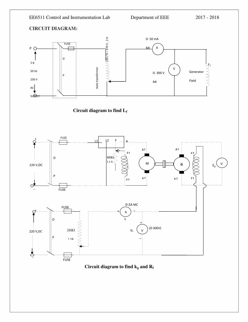
Circuit diagram to find Lf
F1
Generator
Field
Au
to t
ran
sfo
rme
r
23
0 /
0 –
27
0 V
, 2
A
D
P
FUSE
1-
50 Hz
230 V
AC
SUPPLY
A
V
0- 300 V
MI
0- 50 mA
MI P
Eg
FUSE
M
L1 F A
A1
A2
F1
F2
400
1.1 A
D
P
220 V,DC
220 V,DC
SUPPLUY
FUSE
FUSE
V
A
0-2A MC
(0-300V)
Vf 250
1.5A
If
+
+
+
+
_
_
_
_
F1
F2
G
A1
A2
FUSE
D
P
S
Circuit diagram to find kg and Rf
L2
V

EE6511 Control and Instrumentation Lab Department of EEE 2017 - 2018
Ex. No:
Date:
7.(a) DETERMINATION OF TRANSFER FUNCTION OF DC GENERATOR
AIM:
To obtain the transfer function of a seperately excited DC generator.
APPARATUS REQUIRED:
S.No. Item Specification / Range Quantity
1.
2.
3.
4.
5.
6.
Auto transformer
Voltmeters
Ammeter
Rheostat
Tachometer
Starter
1-, 50 Hz
230 V / 0 – 270 V, 6 A
( 0 –300 V ) MI
( 0 – 300 V ) MC
( 0 – 2 A ) MC
( 0 – 50 mA ) MI
400 , 1.1 A
250 , 1.5 A
0 - 1500 rpm
4 point, 10 A
1
1
2
1
1
1
1
1
PRECAUTIONS:
1. The DPSTS should be in off position.
2. The 3-point/4-point starter should be in off position.
3. At the time of starting the motor field rheostat should be in minimum resistance position
and generator field rheostat should be in maximum resistance position.
4. There should not be any load connected to the generator terminals.

EE6511 Control and Instrumentation Lab Department of EEE 2017 - 2018
THEORY:
A DC generator can be used, as a power amplifier in which the power required to
excite the field circuit is lower than the power output rating of the armature circuit. The voltage
induced eg the armature circuit is directly proportional to the product of the magnetic flux, ,
setup by the field and the speed of rotation, , of the armature which is expressed as
eg = k1 ……….. (1.1)
The flux is a function of field current and the type of iron used in the field. A typical
magnetization showing flux as a function of field current is shown in figure
Upto saturation the relation is approximately linear and the flux is directly proportional to field
current i.e.
= k2 if . ………………. (1.2)
Combining both equations,
e.g. = k1 k2 if ………………...(1.3)
When used as a power amplifier the armature is driven at a constant speed and the equation (1.3)
becomes
e.g. = kg if
SLOPE=K1
AMPS FIELD CURRENT
FLUX

EE6511 Control and Instrumentation Lab Department of EEE 2017 - 2018
A generator field winding is represented with Lf and Rf as inductance and resistance of the
field circuit.
The equations for the generator are,
Finding Laplace transform of the equation 1.3 and 1.4,
Combining the above two equations,
Then the transfer function of a DC generator is given as,
)4.1(...............................................................ff
f
ff iRdt
diLe
)5.1.........(..................................................sIRsLsE ffff
)6.1.......(............................................................sIksE fgg
ff
g
f
g
RSL
k
SE
SE
)(
)(
f
g
R
kWhereK
)7.1........(......................................................................
1 ff
g
s
K
sE
sE
f
f
fR
Land
EE6511 Control and Instrumentation Lab Department of EEE 2017 - 2018
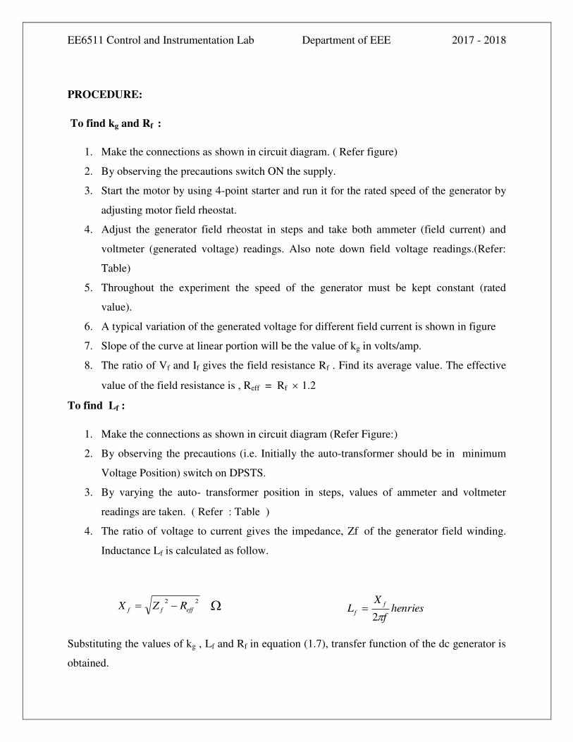
PROCEDURE:
To find kg and Rf :
1. Make the connections as shown in circuit diagram. ( Refer figure)
2. By observing the precautions switch ON the supply.
3. Start the motor by using 4-point starter and run it for the rated speed of the generator by
adjusting motor field rheostat.
4. Adjust the generator field rheostat in steps and take both ammeter (field current) and
voltmeter (generated voltage) readings. Also note down field voltage readings.(Refer:
Table)
5. Throughout the experiment the speed of the generator must be kept constant (rated
value).
6. A typical variation of the generated voltage for different field current is shown in figure
7. Slope of the curve at linear portion will be the value of kg in volts/amp.
8. The ratio of Vf and If gives the field resistance Rf . Find its average value. The effective
value of the field resistance is , Reff = Rf 1.2
To find Lf :
1. Make the connections as shown in circuit diagram (Refer Figure:)
2. By observing the precautions (i.e. Initially the auto-transformer should be in minimum
Voltage Position) switch on DPSTS.
3. By varying the auto- transformer position in steps, values of ammeter and voltmeter
readings are taken. ( Refer : Table )
4. The ratio of voltage to current gives the impedance, Zf of the generator field winding.
Inductance Lf is calculated as follow.
Substituting the values of kg , Lf and Rf in equation (1.7), transfer function of the dc generator is
obtained.
henriesf
XL
f
f 2
22
effff RZX

EE6511 Control and Instrumentation Lab Department of EEE 2017 - 2018
TABULATION:
To find Rf :
S.No.
Field
Voltage
Vf (Volts)
Field
Current
If (Amps)
Field
Resistance
Rf (Ohms)
Generated
Voltage
Eg (volts)
To find Ra:
Sl.No. Ammeter Reading
I (amps)
Voltmeter Reading
V (volts)
Armature
Resistance
Ra (ohms)

EE6511 Control and Instrumentation Lab Department of EEE 2017 - 2018
To find Za:
Sl.No.
Ammeter
Reading
I (amps)
Voltmeter
Reading
V (volts)
Armature
Impedance
Za (ohms)
Xa
(Ohms)
La
(Henry)
MODEL GRAPH:
Field current VS Generated voltage
SLOPE=K1
AMPS FIELD CURRENT
VOLTS
GENERATED
VOLTAGE

EE6511 Control and Instrumentation Lab Department of EEE 2017 - 2018
MODEL CALCULATION:
RESULT:

EE6511 Control and Instrumentation Lab Department of EEE 2017 - 2018
CIRCUIT DIAGRAM:
ARMATURE AND FIELD CONTROLLED DC MOTOR:
TO MEASURE ARMATURE RESISTANCE Ra:

EE6511 Control and Instrumentation Lab Department of EEE 2017 - 2018
Ex. No:
Date:
7.(b) DETERMINATION OF TRANSFER FUNCTION OF DC MOTOR
AIM:
1. To determine the transfer function of an armature controlled DC motor.
2. To determine the transfer function of an field controlled DC motor.
APPARATUS REQUIRED:
Name Range Qty Type Ammeter Voltmeter Auto transformer Rheostat Tachometer Stopwatch
(0-5A),(0-2A),(0-10A), (0-100mA) (0-300V),(0-300V) (0-300V),(0-150V) 1Ф,230V/(0-270V),5A
400Ω,1.1A/50 Ω,3.5A/250 Ω,1.5A
Each 1 Each1 Each1 1 Each1 1 1
MC MC MI
THEORY:
TRANSFER FUNCTION OF ARMATURE CONTROLLED DC MOTOR The differential equations governing the armature controlled |DC motor speed control system are
………………………..1
..……………………..2
…………………………3
…………………………4

EE6511 Control and Instrumentation Lab Department of EEE 2017 - 2018
On taking Laplace transform of the system differential equations with zero initial conditions we
get
………………………5
TO MEASURE FIELD RESISTANCE Rf:
………………………………6
………………………………7
………………………………8
on equating equation 6 and 7
………………………………9
Equation 5 can be written as
………………………………10
Substitute Eb(s) and Ia(s) from eqn 8,9 respectively in equation 10
The required transfer function is

EE6511 Control and Instrumentation Lab Department of EEE 2017 - 2018
Where La / Ra =Ta= electrical time constant
J /B =Tm =mechanical time constant
TRANSFER FUNCTION OF FIELD CONTROLLED DC MOTOR
The differential equations governing the field controlled DC motor speed control system are,
………………………………11
………………………………12
………………………………13
Equation 12 and 13
………………………………14
TO MEASURE ARMATURE INDUCTANCE(La):

EE6511 Control and Instrumentation Lab Department of EEE 2017 - 2018
TO MEASURE FIELD INDUCTANCE( LF):
TO MEASURE Ka
………………………………15
The equation 4 becomes
………………………………16
On substituting If(s) from equation 7 and 8, we get
………………………………17

EE6511 Control and Instrumentation Lab Department of EEE 2017 - 2018
………………………………18
………………………………19
Where
Motor gain constant Km = Ktf /Rfb
Field time constant Tf= Lf/Rf
Mechanical time constant Tm = J/B
PROCEDURE:
To find armature resistance Ra:
1. Connections were given as per the circuit diagram.
2. By varying the loading rheostat take down the readings on ammeter and voltmeter.
3. Calculate the value of armature resistance by using the formula Ra = Va / Ia.
To find armature resistance La:
1. Connections were given as per the circuit diagram.
2. By varying the AE positions values are noted.
3. The ratio of voltage and current gives the impedance Za of the armature reading.
Inductance La is calculated as follows.
To find armature ka:
1. Connections are made as per the circuit diagram.
2. Keep the rheostat in minimum position.
3. Switch on the power supply.

EE6511 Control and Instrumentation Lab Department of EEE 2017 - 2018
4. By gradually increasing the rheostat, increase the motor to its rated speed.
5. By applying the load note down the readings of voltmeter and ammeter.
6. Repeat the steps 4 to 5 times.
To find kb:
1. Connections are made as per the circuit diagram.
2. By observing the precautions switch on the supply.
3. Note down the current and speed values.
4. Calculate Eb and 𝛚.
TO FIND Kb
TABULATION:
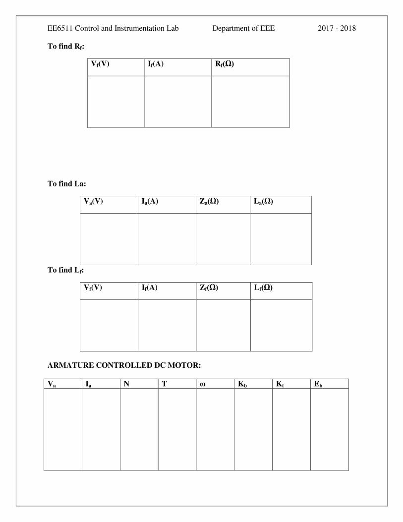
To find Ra:
Va(V) Ia(A) Ra(Ω)
EE6511 Control and Instrumentation Lab Department of EEE 2017 - 2018
To find Rf:
Vf(V) If(A) Rf(Ω)
To find La:
Va(V) Ia(A) Za(Ω) La(Ω)
To find Lf:
Vf(V) If(A) Zf(Ω) Lf(Ω)
ARMATURE CONTROLLED DC MOTOR:
Va Ia N T ω Kb Kt Eb

EE6511 Control and Instrumentation Lab Department of EEE 2017 - 2018
FIELD CONTROLLED DC MOTOR:
Va Ia N Tm ω Eb Km T Ktf Tf
MODEL GRAPH:

EE6511 Control and Instrumentation Lab Department of EEE 2017 - 2018

EE6511 Control and Instrumentation Lab Department of EEE 2017 - 2018
MODEL CALCULATION
RESULT:

EE6511 Control and Instrumentation Lab Department of EEE 2017 - 2018
BLOCK DIAGRAM:

EE6511 Control and Instrumentation Lab Department of EEE 2017 - 2018
Ex. No:
Date:
8(a). DC POSITION CONTROL SYSTEM
AIM:
To control the position of loading system using DC servo motor.
APPARATUS REQUIRED:
S.NO APPARATUS SPECIFICATION QUANTITY
1. DC Servo Motor Position Control Trainer
- 1
3. Connecting Wires - As required
THEORY:
DC Servo Motor Position Control Trainer has consisted various stages. They are Position
set control (TX), Position feed back control (RX), buffer amplifiers, summing amplifiers, error
detector and power drivter circuits. All these stages are assembled in a separate PCB board.
Apart from these, wo servo potentiometers and a dc servomotor are mounted in the separate
assembly. By Jones plug these two assemblies are connected.
The servo potentiometers are different from conventional potentiometers by angle of
rotation. The Normal potentiometers are rotating upto 270. But the servo potentiometers are can
be rotate upto 360. For example, 1K servo potentiometer give its value from o to 1 K for
one complete rotation (360). All the circuits involved in this trainer are constructed by operational amplifiers. For
some stages quad operational amplifier is used. Mainly IC LM 324 and IC LM 310 are used. For
the power driver circuit the power transistors like 2N 3055 and 2N 2955 are employed with
suitable heat sinks.
Servo Potentiometers:
A 1 K servo potentiometer is used in this stage. A + 5 V power supply is connected to this
potentiometer. The feed point of this potentiometer is connected to the buffer amplifiers. A same
value of another servo potentiometer is provided for position feedback control circuit. This
potentiometer is mechanically mounted with DC servomotor through a proper gear arrangement.
Feed point of this potentiometer is also connected to another buffer circuit. To measuring the
angle of rotations, two dials are placed on the potentiometer shafts. When two feed point
voltages are equal, there is no moving in the motor. If the positions set control voltages are
higher than feedback point, the motor will be run in one direction and for lesser voltage it will
run in another direction.
Buffer amplifier for transmitter and receiver and summing amplifier are constructed in one quad
operational amplifier. The error detector is constructed in a single opamp IC LM 310. And
another quad operational amplifier constructs other buffer stages.

EE6511 Control and Instrumentation Lab Department of EEE 2017 - 2018
PROCEDURE:
1. Connect the trainer kit with motor setup through 9 pin D connector.
2. Switch ON the trainer kit.
3. Set the angle in the transmitter by adjusting the position set control as Өs.
4. Now, the motor will start to rotate and stop at a particular angle which is tabulated as Өm.
5. TabulateӨm for different set angle Өs.
6. Calculate % error using the formulae and plot the graph ӨsvsӨm and Өsvs % error.
FORMULA USED:
Error in degree =ϴs - ϴm Error in percentage = ((ϴs - ϴm) / ϴs)* 100
TABULATION:
S. No
Set Angle in degrees(set Өs)
Measured angle in degrees( Өm)
Error in degrees(Өs – Өm
Error in %[(Өs – Өm) / Өs] x 100

EE6511 Control and Instrumentation Lab Department of EEE 2017 - 2018
MODEL GRAPH:
RESULT:
REVIEW QUESTIONS:
1. Which motor is used for position control?
2. Differentiate DC servo motor and DC shunt motor.
3. How the mechanical rotation is converted to electrical signals?
4. What are the time domain specifications?
5. What are the advantages of dc servo motor?

EE6511 Control and Instrumentation Lab Department of EEE 2017 - 2018
BLOCK DIAGRAM :

EE6511 Control and Instrumentation Lab Department of EEE 2017 - 2018
Ex. No:
Date:
8(b). AC POSITION CONTROL SYSTEM
AIM:
To control the position of loading system using AC servo motor.
APPARATUS REQUIRED:
S.NO APPARATUS SPECIFICATION QUANTITY
1. AC Servo Motor Position Control Trainer
- 1
3. Connecting Wires - As required
THEORY:
AC SERVOMOTOR POSITION CONTROL:
It is attempted to position the shaft of a AC Synchronous Motor’s (Receiver) shaft at any
angle in the range of 100 to 3500 as set by the Transmitter’s angular position transducer
(potentiometer), in the range of 100 to 3500. This trainer is intended to study angular position
between two mechanical components (potentiometers), a Transmitter Pot and Receiver pot. The
relation between these two parameters must be studied.
Any servo system has three blocks namely Command, Control and Monitor.
(a) The command is responsible for determining what angular position is desired.. This is
corresponds to a Transmitter’s angular position (Set Point- Sp) set by a potentiometer.
(b) The Control (servo) is an action, in accordance with the command issued and a control is
initiated (Control Variable -Cv) which causes a change in the Motor’s angular position. This
corresponds to the receiver’s angular position using a mechanically ganged potentiometer.
(c) Monitor is to identify whether the intended controlled action is executed properly or not.
This is similar to feedback. This corresponds to Process Variable Pv. All the three actions
together form a closed loop system.
PROCEDURE:
1. Connect the trainer kit with motor setup through 9 pin D connector.
2. Switch ON the trainer kit.
3. Set the angle in the transmitter by adjusting the position set control as Өs.
4. Now, the motor will start to rotate and stop at a particular angle which is tabulated as Өm.
5. Tabulate Өm for different set angle Өs.
6 . Calculate % error using the formulae and plot the graph ӨsvsӨm and Өsvs % error.

EE6511 Control and Instrumentation Lab Department of EEE 2017 - 2018
TABULATION:
S. No
Set Angle in degrees(set Өs)
Measured angle in degrees( Өm)
Error in degrees(Өs – Өm
Error in %[(Өs – Өm) / Өs] x 100
MODEL GRAPH:
RESULT:
REVIEW QUESTIONS:
1. What is meant by Synchro?
2. How the rotor position is controlled in AC position controller?
3. What are the different types of rotor that are used in ac servomotor?
4. What is electrical zero of Synchro?
5. What are the applications of Synchro?

EE6511 Control and Instrumentation Lab Department of EEE 2017 - 2018
Ex. No:
Date:
9.DESIGN OF LEAD, LAG AND LEAD-LAG COMPENSATORS
AIM :
To Design the Lead, Lag and Lead-Lag compensator for the system using MATLAB
Software.
APPARATUS REQUIRED :
1. MATLAB Software.
DESIGN PROCEDURE
1. Design a Phase Lag compensator for the unity feedback transfer function G(s)=K
/s(s+1)(s+4) has specifications : a. Phase Margin>_ 400 b. The steady state error for ramp
input is less than or equal to 0.2 and check the results using MATLAB Software.
Solution
num=[20]
den=[1 5 4 0]
G=tf(num,den)
figure(1);
bode(num,den);
Title('bode plot for uncompensated system G(s)=20/S(S+1)(S+4)')
grid;
[Gm,Pm,Wcp,Wcp]=MARGIN(num,den)
Gmdb=20*log10(Gm);
W=logspace(-1,1,100)';

EE6511 Control and Instrumentation Lab Department of EEE 2017 - 2018
[mag,ph]=BODE(G,W);
ph=reshape(ph,100,1);
mag=reshape(mag,100,1);
PM=-180+40+5
Wg=interp1(ph,W,PM)
beta=interp1(ph,mag,PM)
tau=8/Wg
D=tf([tau 1],[beta*tau 1])
Gc=D*G
figure(2);
bode(Gc);
Title('Bode Plot for the Lag compensated System')
grid;
[Gm1,Pm1,Wcg1,Wcp1]=MARGIN(Gc)
Answers
num = 20
den = 1 5 4 0
Transfer function:
20
-----------------
s^3 + 5 s^2 + 4 s
Gm = 1.0000
Pm = 7.3342e-006

EE6511 Control and Instrumentation Lab Department of EEE 2017 - 2018
Wcp = 2.0000
Wcp = 2.0000
PM = -135
Wg = 0.7016
beta = 5.7480
tau = 11.4025
Transfer function:
11.4 s + 1
-----------
65.54 s + 1
Transfer function:
228 s + 20
---------------------------------------
65.54 s^4 + 328.7 s^3 + 267.2 s^2 + 4 s
Gm1 = 5.2261
Pm1 = 38.9569
Wcg1 = 1.9073
Wcp1 = 0.7053

EE6511 Control and Instrumentation Lab Department of EEE 2017 - 2018
-100
-50
0
50
100
Mag
nitu
de (
dB)
10-2
10-1
100
101
102
-270
-225
-180
-135
-90
Pha
se (
deg)
bode plot for uncompensated system G(s)=20/S(S+1)(S+4)
Frequency (rad/sec)
`
-150
-100
-50
0
50
100
Magnitu
de (
dB
)
10-4
10-3
10-2
10-1
100
101
102
-270
-225
-180
-135
-90
Phase (
deg)
Bode Plot for the Lag compensated System
Frequency (rad/sec)

EE6511 Control and Instrumentation Lab Department of EEE 2017 - 2018
2. Design a Phase Lead compensator for the unity feedback transfer function G(s)=K
/s(s+2) has specifications : a. Phase Margin>_ 550 b. The steady state error for ramp
input is less than or equal to 0.33 and check the results using MATLAB Software. (Assume
K=1)
Solution
num=[5]
den=[1 2 0]
G=tf(num,den)
figure(1);
bode(num,den);
Title('Bode Plot for uncompensated system G(s)=5/s(s+2)')
grid;
[Gm,Pm,Wcg,Wcp]=MARGIN(num,den)
GmdB=20*log10(Gm)
PM=55-Pm+3
alpha=(1-sin(PM*pi/180))/(1+sin(PM*pi/180))
Gm=-20*log10(1/sqrt(alpha))
w=logspace(-1,1,100)';
[mag1,phase1]=BODE(num,den,w);
mag=20*log10(mag1);
magdB=reshape(mag,100,1);

EE6511 Control and Instrumentation Lab Department of EEE 2017 - 2018
Wm=interp1(magdB,w,-20*log10(1/sqrt(alpha)))
tau=1/(Wm*sqrt(alpha))
D=tf([tau 1],[alpha*tau 1])
Gc=D*G
figure(2);
bode(Gc);
Title('Bode Plot for the Lead Compensated System')
grid;
[Gm1,Pm1,Wcg1,Wcp1]=MARGIN(Gc)
Answers
num = 5
den = 1 2 0
Transfer function:
5
---------
s^2 + 2 s
Gm = Inf
Pm = 47.3878
Wcg = Inf
Wcp = 1.8399
GmdB = Inf
PM = 10.6122
alpha = 0.6890
Gm = -1.6181

EE6511 Control and Instrumentation Lab Department of EEE 2017 - 2018
Wm = 2.0853
tau = 0.5777
Transfer function:
0.5777 s + 1
------------
0.398 s + 1
Transfer function:
2.889 s + 5
---------------------------
0.398 s^3 + 1.796 s^2 + 2 s
Gm1 = Inf
Pm1 = 54.4212
Wcg1 = Inf
Wcp1 = 2.0849
-80
-60
-40
-20
0
20
40
Mag
nitu
de (
dB)
10-1
100
101
102
-180
-135
-90
Pha
se (
deg)
Bode Plot for uncompensated system G(s)=5/s(s+2)
Frequency (rad/sec)

EE6511 Control and Instrumentation Lab Department of EEE 2017 - 2018
-80
-60
-40
-20
0
20
40
Mag
nitu
de (
dB)
10-1
100
101
102
-180
-135
-90
Pha
se (
deg)
Bode Plot for the Lead Compensated System
Frequency (rad/sec)
3. Design a Phase Lead-lag compensator for the unity feedback transfer function G(s)=K
/s(s+1)(s+2) has specifications : a. Phase Margin>_ 500 b. The Velocity error constant
Kv=10 sec-1 and check the results using MATLAB Software. (Assume K=1).
Solution
num=[20]
den=[1 3 2 0]
G=tf(num,den)
figure(1);
bode(num,den);
Title('bode Plot for Uncompensated System G(s)=20/S(S+1)(S+2)')
grid;

EE6511 Control and Instrumentation Lab Department of EEE 2017 - 2018
[Gm,Pm,Wcg,Wcp]=MARGIN(num,den)
GmdB=20*log10(Gm);
W=logspace(-1,1,100)';
%Bode Plot for Lag Section
[mag,ph]=BODE(G,W);
ph=reshape(ph,100,1);
mag=reshape(mag,100,1);
PM=-180+50+5
Wg=interp1(ph,W,PM)
beta=interp1(ph,mag,PM)
tau=8/Wg
D=tf([tau 1],[beta*tau 1])
%Bode Plot for Lead section
alpha=20/beta
mag=20*log10(mag)
Gm=-20*log10(1/sqrt(alpha))
Wm=interp1(mag,W,-20*log10(1/sqrt(alpha)))
tau=1/(Wm*sqrt(alpha))
E=tf([tau 1],[alpha*tau 1])
Gc1=D*E*G
figure(2);

EE6511 Control and Instrumentation Lab Department of EEE 2017 - 2018
bode(Gc1);
Title('Bode Plot for the Lag-lead compensated System')
grid;
grid;
[Gm1,Pm1,Wcg1,Wcp1]=MARGIN(Gc1)
Answers
num = 20
den = 1 3 2 0
Transfer function:
20
-----------------
s^3 + 3 s^2 + 2 s
Gm = 0.3000
Pm = -28.0814
Wcg = 1.4142
Wcp = 2.4253
PM = -125
Wg = 0.4247
beta = 21.2032
tau = 18.8362
Transfer function:
18.84 s + 1
-----------
399.4 s + 1
alpha = 0.9433

EE6511 Control and Instrumentation Lab Department of EEE 2017 - 2018
Gm = -0.2537
Wm = 2.4546
tau = 0.4195
Transfer function:
0.4195 s + 1
------------
0.3957 s + 1
Transfer function:
158 s^2 + 385.1 s + 20
------------------------------------------------
158 s^5 + 873.9 s^4 + 1516 s^3 + 802.6 s^2 + 2 s
Gm1 = 6.1202
Pm1 = 48.5839
Wcg1 = 1.3976
Wcp1 = 0.4279
-100
-50
0
50
100
Mag
nitu
de (d
B)
10-2
10-1
100
101
102
-270
-225
-180
-135
-90
Phas
e (d
eg)
bode Plot for Uncompensated System G(s)=20/S(S+1)(S+2)
Frequency (rad/sec)

EE6511 Control and Instrumentation Lab Department of EEE 2017 - 2018
-150
-100
-50
0
50
100
150
Mag
nitu
de (
dB)
10-4
10-3
10-2
10-1
100
101
102
-270
-225
-180
-135
-90
Pha
se (
deg)
Bode Plot for the Lag-lead compensated System
Frequency (rad/sec)
RESULT
Thus the design of compensator can be designed for Lead, Lag and Lead-Lag for the
given system using MATLAB Software.

EE6511 Control and Instrumentation Lab Department of EEE 2017 - 2018
Ex. No:
Date:
10. SIMULATION OF CONTROL SYSTEM AND STABILITY ANALYSIS
AIM :-
To Check the stability analysis of the given system or transfer function using MATLAB
Software.
APPARATUS REQUIRED
1. MATLAB Software
DESIGN PROCEDURE :
1. Root Locus : The open loop transfer function of a unity feedback system
G(s)=K/s(s2+8s+17) Draw the root locus manually and Check the same results using
MATLAB Software. (Assume K=1)
Solution
% Rootlocus of the transfer function G(s)=1/(S^3+8S^2+17S)
num=[1];
den=[1 8 17 0];
figure(1);
rlocus(num,den);
Title('Root Locus for the transfer function G(s)=1/(S^3+8S^2+17S)')
grid;

EE6511 Control and Instrumentation Lab Department of EEE 2017 - 2018
-14 -12 -10 -8 -6 -4 -2 0 2 4-10
-8
-6
-4
-2
0
2
4
6
8
10
0.92
0.98
0.160.30.460.60.720.84
0.92
0.98
2468101214
0.160.30.460.60.720.84
Root Locus for the transfer function G(s)=1/(S3+8S2+17S)
Real Axis
Imag
inar
y A
xis
2. BODE PLOT : The open loop transfer function of a unity feedback system
G(s)=K/s(s2+2s+3) Draw the Bode Plot manually Find (i)Gain Margin (ii)Phase Margin
(iii)Gain cross over frequency (iv)Phase cross over frequency (v) Resonant Peak
(vi)Resonant Frequency (vii)Bandwidth and Check the same results using MATLAB
Software. (Assume K=1)
Solution
%Draw the Bode Plot for the given transfer functionG(S)=1/S(S2+2S+3) %Find (i)Gain Margin
(ii) Phase Margin (iii) Gain Cross over Frequency %(iv) Phase Cross over Frequency
(v)Resonant Peak (vi)Resonant %Frequency (vii)Bandwidth
num=[1 ];
den=[1 2 3 0];
w=logspace(-1,3,100);
figure(1);

EE6511 Control and Instrumentation Lab Department of EEE 2017 - 2018
bode(num,den,w);
title('Bode Plot for the given transfer function G(s)=1/s(s^2+2s+3)')
grid;
[Gm Pm Wcg Wcp] =margin(num,den);
Gain_Margin_dB=20*log10(Gm)
Phase_Margin=Pm
Gaincrossover_Frequency=Wcp
Phasecrossover_Frequency=Wcg
[M P w]=bode(num,den);
[Mp i]=max(M);
Resonant_PeakdB=20*log10(Mp)
Wp=w(i);
Resonant_Frequency=Wp
for i=1:1:length(M);
if M(i)<=1/(sqrt(2));
Bandwidth=w(i)
break;
end;
end;
Answer

EE6511 Control and Instrumentation Lab Department of EEE 2017 - 2018
-200
-150
-100
-50
0
50
Mag
nitud
e (d
B)
10-1
100
101
102
103
-270
-225
-180
-135
-90
Phas
e (d
eg)
Bode Plot for the given transfer function G(s)=1/s(s2+2s+3)
Frequency (rad/sec)
Gain_Margin_dB =15.5630
Phase_Margin = 76.8410
Gaincrossover_Frequency = 0.3374
Phasecrossover_Frequency= 1.7321
Resonant_PeakdB = 10.4672
Resonant_Frequency = 0.1000
Bandwidth = 0.5356
3. Nyquist Plot : The open loop transfer function of a unity feedback system
G(s)=K/s(s2+2s+3) Draw the Nyquist Plot manually Find (i)Gain Margin (ii)Phase Margin
(iii)Gain cross over frequency (iv)Phase cross over frequency and Check the same results
using MATLAB Software. (Assume K=1)
Solution
%Nyquist Plot for the Transfer Function G(s)=1/(s+1)^3
num=[1];

EE6511 Control and Instrumentation Lab Department of EEE 2017 - 2018
den=[1 3 3 1];
figure(1);
nyquist(num,den)
Title('Nyquist Plot for the Transfer Function G(s)=1/(s+1)^3')
[Gm,Pm,Wcg,Wcp] =margin(num,den)
grid;
[Gm,Pm,Wcg,Wcp] =margin(num,den);
Gain_Margin=Gm
Phase_Margin=Pm
PhaseCrossover_Frequency=Wcg
GainCrossover_Frequency=Wcp
-1 -0.8 -0.6 -0.4 -0.2 0 0.2 0.4 0.6 0.8 1-1
-0.8
-0.6
-0.4
-0.2
0
0.2
0.4
0.6
0.8
1
0 dB
-20 dB
-10 dB
-6 dB
-4 dB-2 dB
20 dB
10 dB
6 dB
4 dB2 dB
Nyquist Plot for the Transfer Function G(s)=1/(s+1)3
Real Axis
Imag
inary
Axis
Answer

EE6511 Control and Instrumentation Lab Department of EEE 2017 - 2018
Gain_Margin = 8.0011
Phase_Margin = -180
PhaseCrossover_Frequency = 1.7322
GainCrossover_Frequency = 0
4. Nichols Chart : The open loop transfer function of a unity feedback system G(s)=60
/s(s+2)(s+3) Draw the Nichol’s Chart manually Find (i)Gain Margin (ii)Phase Margin
(iii)Gain cross over frequency (iv)Phase cross over frequency (v) Resonant Peak
(vi)Resonant Frequency (vii)Bandwidth and Check the results using MATLAB Software.
(Assume K=1)
Solution
num=[60];
den=[1 8 12 0];
figure(1);
nichols(num,den)
Title('Nichols Plot for the Transfer Function G(s)=60/s(s+2)(s+6)')
grid;
[Mag,Ph,w] =bode(num,den);
[Gm,Pm,Wcg,Wcp] =margin(num,den);
Gain_Margin=Gm
GainMargin_dB=20*log10(Gm)
Phase_Margin=Pm
PhaseCrossover_Frequency=Wcg
GainCrossover_Frequency=Wcp

EE6511 Control and Instrumentation Lab Department of EEE 2017 - 2018
[Mp,k] =max(Mag);
Resonant_Peak=Mp;
Resonant_PeakdB=20*log10(Gm)
Resonant_Frequency=w(k)
% In Nichol’s Chart the bandwidth is obtained in -3dB
n=1;
while 20*log10(Mag(n))>=-3
n=n+1;
end;
Bandwidth=w(n)
Answer
GainMargin_dB = 4.0824
Phase_Margin = 12.1738
PhaseCrossover_Frequency = 3.4641
GainCrossover_Frequency = 2.7070
Resonant_PeakdB = 4.0824
Resonant_Frequency = 0.1000
Bandwidth = 3.4641

EE6511 Control and Instrumentation Lab Department of EEE 2017 - 2018
-360 -315 -270 -225 -180 -135 -90 -45 0-120
-100
-80
-60
-40
-20
0
20
40
60
6 dB 3 dB
1 dB 0.5 dB
0.25 dB 0 dB
-1 dB
-3 dB
-6 dB
-12 dB
-20 dB
-40 dB
-60 dB
-80 dB
-100 dB
-120 dB
Nichols Plot for the Transfer Function G(s)=60/s(s+2)(s+6)
Open-Loop Phase (deg)
Ope
n-Lo
op G
ain
(dB
)
RESULT
Thus the given system or Transfer function stability analysis can be obtained through
MATLAB Software using Root Locus, Nyquist Plot, Nichol’s Chart and Bode plot.

EE6511 Control and Instrumentation Lab Department of EEE 2017 - 2018
Ex. No:
Date:
11. PROCESS SIMULATION
AIM :
To Check the process simulation result with First Order and Second Order System wit the
step input.
APPARATUS REQUIRED:
1. MATLAB Software.
DESIGN OF SIMULINK BLOCK
1.First Order System
1
s+1
Transfer FcnStep Scope

EE6511 Control and Instrumentation Lab Department of EEE 2017 - 2018
2. Second Order System
1. Critically Damped System
25
s +10s+252
Transfer FcnStep Scope

EE6511 Control and Instrumentation Lab Department of EEE 2017 - 2018
2. Under Damped System
25
s +2s+252
Transfer FcnStep Scope
EE6511 Control and Instrumentation Lab Department of EEE 2017 - 2018
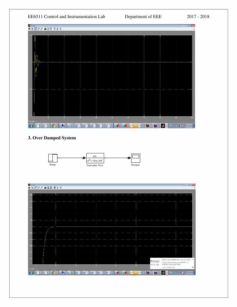
3. Over Damped System
25
s +15s+252
Transfer FcnStep Scope

EE6511 Control and Instrumentation Lab Department of EEE 2017 - 2018
4. UnDamped System
25
s +252
Transfer FcnStep Scope
1. The Second order system has the transfer functions (i)Under Damped Second Order
System G(s)=10/(s2+2s+10) (ii) Undamped Second Order system G(s)=10/(s2+10)
(iii)Critically Damped Second Order System G(s)=10/(s2+7.32s+10) (iv)Over Damped
Second Order System
G(s)=10/(s2+3s+10) for that apply step input and check the result 4-cases using MATLAB
Software.
ANS
% Time Domain Specifications
num1=[10];
den1=[1 2 10];

EE6511 Control and Instrumentation Lab Department of EEE 2017 - 2018
%Transfer Function Form
G=tf(num1,den1)
% Natural frequency and Damping Ratio
[Wn Z P] = damp(G)
Wn=Wn(1);
Z=Z(1);
t=0:0.1:20
%(i) Under Damped System For Step Input
figure(1);
step(num1,den1,t)
title('Under Damped Second Order System Response for Step Input');
grid;
0 0.5 1 1.5 2 2.5 3 3.5 4 4.5 5-1
-0.5
0
0.5
1
1.5
2
2.5Impulse input for the Second Order System
Time in Seconds (sec)
Am
plitu
de o
f Im
puls
e In
put

EE6511 Control and Instrumentation Lab Department of EEE 2017 - 2018
% (ii) Undamped Second Order System has the T.F=10/(S^2+10) with the Damping ratio=0 for
Step Input
num2=[10];
den2=[1 0 10];
figure(2);
step(num2,den2,t)
title('Undamped Second Order System Response for Step Input');
grid;
0 0.5 1 1.5 2 2.5 3 3.5 4 4.5 50
0.2
0.4
0.6
0.8
1
1.2
1.4Step input for the Second Order System
Time in Seconds (sec)
Am
plit
ude o
f S
tep Input

EE6511 Control and Instrumentation Lab Department of EEE 2017 - 2018
% (iii) Critically damped Second Order System has the T.F=10/(S^2+7.32*s+10) with the
Damping ratio=1 for step input
num3=[10];
den3=[1 7.32 10];
figure(3);
step(num3,den3,t)
title('Critically Damped Second Order System Response for Step Input');
grid;
0 0.5 1 1.5 2 2.5 3 3.5 4 4.5 50
0.5
1
1.5
2
2.5
3
3.5
4
4.5
5Ramp input for the Second Order System
Time in Seconds
Am
plitu
de o
f R
am
p I
nput
and S
yste
m O
utp
ut
Unit Ramp Input
Ramp output response

EE6511 Control and Instrumentation Lab Department of EEE 2017 - 2018
(iv) Critically damped Second Order System has the T.F=10/(S^2+3*s+10)with the Damping
ratio=1.5 for step input
num4=[10];
den4=[1 3 10];
figure(4);
step(num4,den4,t)
title('Over Damped Second Order System Response for Step Input');
grid;
0 0.5 1 1.5 2 2.5 3 3.5 4 4.5 50
2
4
6
8
10
12
14 Acceleration or Parabolic input for the Second Order System
Time in Seconds
Am
plit
ude o
f A
ccele
ration
Input
and S
yste
m O
utp
ut
Unit Acceleration Input
Acceleration output response
RESULT :
Thus the Simulation Results are obtained through MATLAB Software Through First
Order System and Second Order System with Step input.

EE6511 Control and Instrumentation Lab Department of EEE 2017 - 2018
Ex. No:
Date:
12. TIME DOMAIN AND FREQUENCY DOMAIN
SPECIFICATIONS
AIM
To obtain the time domain and Frequency Domain Specifications for the given system
using MATLAB Software.
APPARATUS REQUIRED
1. MATLAB Software
DESIGN PROCEDURE :
1. The open loop transfer function G(s)=100/s(s+15) has a unity feedback. Find (i) Natural
Frequency and Damping Ratio (ii)Position, Velocity, Acceleration Error Constants
(iii)Damped Frequency and Theta (iv)Delay Time (v) Rise Time (vi)Peak Time
(vii)Maximum Peak over shoot percentage (viii) Settling Time for 2% and 5% and
Calculate the same results using MATLAB Software.
Solution
% Time Domain Specifications
num=[100];
den=[1 15 0];
%Transfer Function Form
G=tf(num,den)
% Unity Feedback System
C=feedback(G,1)
% (i)Natural frequency and Damping Ratio

EE6511 Control and Instrumentation Lab Department of EEE 2017 - 2018
[Wn Z P] = damp(C)
Wn=Wn(1);
Z=Z(1);
%(ii)Position,Velocity,Acceleration Error Constants
% Position Error Constant
Kp=dcgain(G)
%Differentiator Part
num1=[1 0];den1=[1];G1=tf(num1,den1);
%Velocity Error Constant
Gv=G1*G;
Kv=dcgain(Gv)
% Acceleration Error Constant
Ga=Gv*G1;
Ka=dcgain(Ga)
%(iii) Damped Frequency and Theta
% Damped Frequency of oscillation
Wd=Wn*sqrt(1-(Z^2))
%Angle of Theta
Theta=atan((sqrt(1-(Z^2)))/Z)
%(iv)Delay Time(Td)
Td=(1+0.7*Z)/Wn

EE6511 Control and Instrumentation Lab Department of EEE 2017 - 2018
%(v)Rise Time
Tr=(3.14-Theta)/Wd
%(vi)Peak Time
Tp=3.14/Wd
%(vii)Percentage of Peak over shoot
MpPercentage=exp((-3.14*Z)/(sqrt(1-Z^2)))*100
%(viii) Settling Time
% For 2%
Ts=4/(Z*Wn)
% For 5%
Ts=3/(Z*Wn)
Answer
Transfer function:
100
----------
s^2 + 15 s
Transfer function:
100
----------------
s^2 + 15 s + 100

EE6511 Control and Instrumentation Lab Department of EEE 2017 - 2018
(i)Wn = 10.0000
10.0000
Z = 0.7500
0.7500
P = -7.5000 + 6.6144i
-7.5000 - 6.6144i
(ii) Kp = Inf
Kv = 6.6667
Ka = 0
(iii)Wd = 6.6144
Theta= 0.7227
(iv) Td = 0.1525
(v) Tr = 0.3655
(vi) Tp = 0.4747
(vii)MpPercentage = 2.8427
(viii) Ts = 0.5333
Ts = 0.4000

EE6511 Control and Instrumentation Lab Department of EEE 2017 - 2018
2. The open loop transfer function of a unity feedback system G(s)=K/s(s2+2s+3) Draw the
Bode Plot manually Find (i)Gain Margin (ii)Phase Margin (iii)Gain cross over frequency
(iv)Phase cross over frequency (v) Resonant Peak (vi)Resonant Frequency (vii)Bandwidth
and Check the same results using MATLAB Software. (Assume K=1)
Solution
%Draw the Bode Plot for the given transfer functionG(S)=1/S(S2+2S+3) %Find (i)Gain Margin
%(ii) Phase Margin (iii) Gain Cross over Frequency %(iv) Phase Cross over Frequency
%(v)Resonant Peak (vi)Resonant %Frequency (vii)Bandwidth
num=[1 ];
den=[1 2 3 0];
w=logspace(-1,3,100);
figure(1);
bode(num,den,w);
title('Bode Plot for the given transfer function G(s)=1/s(s^2+2s+3)')
grid;
[Gm Pm Wcg Wcp] =margin(num,den);
Gain_Margin_dB=20*log10(Gm)
Phase_Margin=Pm
Gaincrossover_Frequency=Wcp
Phasecrossover_Frequency=Wcg
[M P w]=bode(num,den);
[Mp i]=max(M);
Resonant_PeakdB=20*log10(Mp)
Wp=w(i);
Resonant_Frequency=Wp
for i=1:1:length(M);

EE6511 Control and Instrumentation Lab Department of EEE 2017 - 2018
if M(i)<=1/(sqrt(2));
Bandwidth=w(i)
break;
end;
end;
Answer
-200
-150
-100
-50
0
50
Mag
nitu
de (
dB)
10-1
100
101
102
103
-270
-225
-180
-135
-90
Pha
se (
deg)
Bode Plot for the given transfer function G(s)=1/s(s2+2s+3)
Frequency (rad/sec)
Gain_Margin_dB =15.5630
Phase_Margin = 76.8410
Gaincrossover_Frequency = 0.3374
Phasecrossover_Frequency= 1.7321
Resonant_PeakdB = 10.4672
Resonant_Frequency = 0.1000
Bandwidth = 0.5356

EE6511 Control and Instrumentation Lab Department of EEE 2017 - 2018
MODEL CALCULATION
RESULT:

EE6511 Control and Instrumentation Lab Department of EEE 2017 - 2018
Ex. No:
Date:
13.P, PI, PID CONTROLLERS
AIM: To study the response of the electronic PID controller and derive transfer function. APPARATUSREQUIRED:
PID control Trainer Kit
THEORY:
The input from the PID controller to a system is given by the equation dt
deKdteKeKu dip
Where
pK =Proportional Gain, iK = Integral Gain, dK = Derivative Gain
The transfer function of the PID controller is )()(
)(SKS
KK
sesu
d
ip
This error signal (e) will be sent to the PID controller and the controller output is obtained. MATHEMATICAL FORMULATION:
The gain for the proportional part is calculated using1
2R
RK p
The integral gain is ii
i CRK 1
The derivative gain is ddd CRK
PID CIRCUIT DIAGRAM

EE6511 Control and Instrumentation Lab Department of EEE 2017 - 2018
PROCEDURE:
A. To study the behavior of Proportional Block
1. Connect potentiometer output to the proportional block input.
2. Set gain at 1
3. Connect CRO Channel 1 to the input and Channel 2 to the proportional block
output
4. Vary the potentiometer and observe the proportional response with respect to the
input.
5. Increase gain in steps of 1 and observe the output
6. Here R1=1KΩ and R2 can be varied in steps of 1KΩ.
B. To study the behavior of Integral Block
1. Connect potentiometer output to the integral block input
2. Set gain at 1
3. Connect CRO Channel 1 to the input and channel 2 to the integral block output
4. Vary the potentiometer and observe the integral response with respect to the input
5. Increase gain in steps of 1 and observe the output
6. Here is fixed at 33nF and can be varied in steps of 100Ω
C. To study the behavior of Derivative Block
1. Connect potentiometer output to the derivative block inpu
2. Set at minimum position
3. Connect CRO Channel 1 to the input and channel 2 to the derivative block output
4. Vary the potentiometer and observe the derivative response with respect to the
input
5. Now vary the potentiometer and observe the output
6. Here is fixed at 33nF and can be varied up to 10K

EE6511 Control and Instrumentation Lab Department of EEE 2017 - 2018
D. To study PID response for step input
1. Make connections as per the connection diagram A simple Lag circuit is given in
the connection diagram
2. Set at 1
3. Set at 1
4. Set at minimum position
5. Connect CRO channel 1 to the input and channel 2 at process output i.e., Feedback
6. Observe the PID wave form in the channel 2.
7. Now vary the three gains and observe the response
8. It can be observed that the derivative effect is very less comparatively with and
.
9. Now set the at the center position so that the is at 5K
10. Set different values of and and derive the transfer functions.
11. Make a graph as observed in Oscilloscope.
RESULT:

EE6511 Control and Instrumentation Lab Department of EEE 2017 - 2018
Synchro Transmitter stator angle Vs receiver rotor angle characteristics

EE6511 Control and Instrumentation Lab Department of EEE 2017 - 2018
Ex. No:
Date:
14. SYNCHRO TRANSMITTER & RECEIVER CHARACTERISTICS
AIM:
1. To study the operation of synchro transmitter and receiver as a error detector
2. To study the operation of Synchro Transmitter and Receiver.
APPARATUSREQUIRED:
Synchro transmitter and receiver kit
Patch cords
PROCEDURE:
Synchro transmitter and receiver as an error detector
1. Connect the R1-R2 terminals of transmitter to power supply.
2. Short S1-S2, S2-S2, S3-S3 winding of transmitter and receiver.
3. Connect the R1-R2 terminals of receiver to digital panel meter.
4. As the power is switched ON transmitter and receiver shaft will come to the same
position on the dial.
5. Set the transmitter rotor in zero position and rotate the receiver rotor.
6. Take the error voltage display on the digital panel meter corresponding to the angle
difference between transmitter and receiver.
7. Tabulate the reading as per the following table.
Synchro Transmitter and Receiver
1. Arrange power supply, synchro transmitter and synchro receiver near to each other.
2. Connect power supply output to R1-R2 terminals of the transmitter and receiver.
3. Short S1-S2, S2-S2, and S3-S3 winding of transmitter and receiver with the help of
patch cords.
4. Switch on the unit, supply neon will glow on.
5. As the power is switched on transmitter and receiver shaft will come to the same
position on the dial.
6. Vary the shaft position of the transmitter and observe the corresponding change in
the shaft position of the receiver.
7. Repeat the above steps for different angles of the shaft of the transmitter, you
should have observed that the receiver shaft move by an equal amount as that of a
transmitter.

EE6511 Control and Instrumentation Lab Department of EEE 2017 - 2018

EE6511 Control and Instrumentation Lab Department of EEE 2017 - 2018
Synchro transmitter and receiver angle difference Vs output error voltage
Tabulation for rotor angle versus receiver angle
Transmitter angular
position (degrees)
Receiver angular
position (degrees)
Model Graph

EE6511 Control and Instrumentation Lab Department of EEE 2017 - 2018
Tabulation for error voltage Vs difference between transmitter and receiver rotor angle
Transmitter
position
(degrees)
Receiver
position
(degrees)
Error output
voltage (Volts)
Angle of
difference(degrees)
Model Graph

EE6511 Control and Instrumentation Lab Department of EEE 2017 - 2018
MODEL CALCULATION
RESULT:

EE6511 Control and Instrumentation Lab Department of EEE 2017 - 2018
BEYOND THE SYLLABUS EXPERIMENTS:
Ex. No. 15. Determination of transfer function of AC Servomotor
Date:
Aim:
To derive the transfer function of the given A.C Servo Motor and experimentally determine the transfer function parameters such as motor constant k1 and k2.
Apparatus required:
S.No Apparatus Quantity
1 Transfer function of AC servomotor trainer kit 1
2 Two phase AC servomotor with load setup and loads 1
3 PC power chord 2
4 SP6 patch chord 4
5 9 pin cable 1
Specifications of AC Servomotor
Main winding Voltage - 230V
Control Winding Voltage - 230V
No load current per phase - 300 mA
Load current per phase - 350 mA
Input power - 100 W
Power Factor - 0.8
No load speed - 1400 rpm

EE6511 Control and Instrumentation Lab Department of EEE 2017 - 2018
Full load speed - 900 rpm
Moment of inertia (J) - 0.0155 kg m2
Viscous friction co-efficient (B) - 0.85 x 10⁻⁴ kg-m-sec
Formula Used:
Torque T = (9.18 x r x S) Nm
1 2
Where ,
r - Radius of the shaft, m = 0.0186 m
- Change in torque, Nm
- Change in control winding voltage , V
- Change in speed , rpm
S - Applied load in kg
Theory:
It is basically a 2Φ induction motor except for certain special design features. AC
servomotor differs in 2 ways from a normal induction motor. The servomotor rotor side is built
in high resistance. So the X/R ratio is small, which results in linear mechanical characteristics.
Another difference of AC servomotor is that excitation voltage applied to 2 stator of winding
should have a phase difference of 90o.
Working principle:
When the rotating magnetic field swaps over the rotor conductors emf is induced in the
rotor conductors. This induced emf circulates current in the short circuited rotor conductor. This
rotor current generate a rotor flux a mechanical force is developed to the rotor and hence the
rotor moving the same direction as that of the rotating magnetic field.

EE6511 Control and Instrumentation Lab Department of EEE 2017 - 2018
Transfer function of a AC servomotor
Let Tm – Torque developed by the motor (Nm)
T1 – Torque developed by the load (Nm)
k1 – Slope of control phase voltage versus torque characteristics
k2 – Slope of speed torque characteristics
km – Motor gain constant
τm – Motor time constant
g – Moment of inertia (Kgm-2)
B – Viscous friction co-efficient (N/m/sec)
ec – Rated input voltage, volt
– Angular speed
Transfer function of AC servomotor:
Torque developed by motor, Tm = - …………………….. (1)
Load torque, Tl = ……………………………………..(2)
At equilibrium, the motor torque is equal to the load torque.
- = ………………………………..(3)
On taking laplace transform of equation (3), with zero initial conditions, we get

EE6511 Control and Instrumentation Lab Department of EEE 2017 - 2018
Where = Motor gain constant
= Motor time constant

EE6511 Control and Instrumentation Lab Department of EEE 2017 - 2018
Speed torque characteristics of Induction motor and AC servomotor:
\

EE6511 Control and Instrumentation Lab Department of EEE 2017 - 2018
To find K1 :

EE6511 Control and Instrumentation Lab Department of EEE 2017 - 2018
Connection Procedure:
1. Initially keep all the switches in OFF position
2. Connect the banana connector Pout to Pin and Nout to Nin
3. The banana connector Pin terminal is also connected with motor control winding P
terminal and the banana connector Nin terminal is also connected with motor control
winding N terminal.
4. Connect the 9 pin D connector from AC servomotor to module trainer kit.
5. Keep the variable AC source in minimum position.
Experimental Procedure to find K1:
1. Apply 3-phase AC supply to 3-phase input banana connectors at the back side of the
module.
2. Switch ON the power switch.
3. Switch ON the control winding and main winding switches S1 and S2 respectively.
4. Now slowly vary the variable AC source to the control winding till the motor reaches
300rpm.
5. Apply load one by one till the motor stops.
6. Note down the load values and control voltage.
7. Now again vary the AC source and apply voltage to control winding till the motor
reaches 300 rpm.
8. Again apply loads till the motor stops.
9. Repeat the above steps and note down the values and tabulate it.
10. Calculate the torque of the motor.
11. Draw a graph between control voltage Vs torque.
12. From the graph find out the motor constant K1.

EE6511 Control and Instrumentation Lab Department of EEE 2017 - 2018
Experimental Procedure to find K2:
1. Switch ON the power supply.
2. Switch ON the main winding power supply S2.
3. After giving the power supply to the main winding, switch ON the control winding power
supply switch S1.
4. Vary the control voltage to set a rated voltage of the control winding ( 180 V)
5. Apply the load in step by step upto the motor run at a zero rpm and note down the speed
of the motor and applied load.
6. After taking the readings, fully remove the load from the motor and bring the variable AC
source in minimum position.
7. Switch OFF the control winding switch S1.
8. Finally switch OFF the main winding switch S2 and power supply switch.
9. Tabulate the speed and load values and calculate torque.
10. Draw a graph of torque Vs speed and find motor constant K2.

EE6511 Control and Instrumentation Lab Department of EEE 2017 - 2018
To find K2 :

EE6511 Control and Instrumentation Lab Department of EEE 2017 - 2018
RESULT:

EE6511 Control and Instrumentation Lab Department of EEE 2017 - 2018
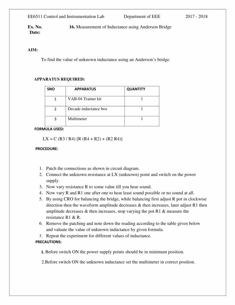
EE6511 Control and Instrumentation Lab Department of EEE 2017 - 2018
Ex. No. 16. Measurement of Inductance using Anderson Bridge Date:
AIM:
To find the value of unknown inductance using an Anderson’s bridge.
APPARATUS REQUIRED:
FORMULA USED:
LX = C (R3 / R4) [R (R4 + R2) + (R2 R4)]
PROCEDURE:
1. Patch the connections as shown in circuit diagram.
2. Connect the unknown resistance at LX (unknown) point and switch on the power
supply.
3. Now vary resistance R to some value till you hear sound.
4. Now vary R and R1 one after one to hear least sound possible or no sound at all.
5. By using CRO for balancing the bridge, while balancing first adjust R pot in clockwise
direction then the waveform amplitude decreases & then increases, later adjust R1 then
amplitude decreases & then increases, stop varying the pot R1 & measure the
resistance R1 & R.
6. Remove the patching and note down the reading according to the table given below
and valuate the value of unknown inductance by given formula.
7. Repeat the experiment for different values of inductance.
PRECAUTIONS:
1. Before switch ON the power supply points should be in minimum position.
2.Before switch ON the unknown inductance set the multimeter in correct position.
SNO APPARATUS QUANTITY
1 VAB-04 Trainer kit 1
2 Decade inductance box 1
3 Multimeter 1

EE6511 Control and Instrumentation Lab Department of EEE 2017 - 2018
TABULATION:
SNO R2 (Ω) R3(Ω) R4(Ω) R (Ω) R1
(Ω) INDUCTANCE(mH)
THEORITICAL PRACTICAL
MODEL GRAPH:
THEORITICAL VALUE LX
PRACTICAL
VALUE LX

EE6511 Control and Instrumentation Lab Department of EEE 2017 - 2018
MODEL CALCULATIONS:
Result:
DISCUSSION QUESTION:
1. What is meant by Anderson Bridge?
2. Differentiate Maxwell’s & Anderson Bridge.
3. What are the advantage & disadvantage of Anderson Bridge?
4. Differentiate the Hay’s & Anderson Bridge.

EE6511 Control and Instrumentation Lab Department of EEE 2017 - 2018